Robust facility location under demand location uncertainty€¦ · Robust facility location under...
52
Robust facility location under demand location uncertainty by Auyon Siddiq A thesis submitted in conformity with the requirements for the degree of Master of Applied Science Graduate Department of Mechanical and Industrial Engineering University of Toronto c Copyright 2013 by Auyon Siddiq
Transcript of Robust facility location under demand location uncertainty€¦ · Robust facility location under...

Robust facility location under demand locationuncertainty
by
Auyon Siddiq
A thesis submitted in conformity with the requirementsfor the degree of Master of Applied Science
Graduate Department of Mechanical and Industrial EngineeringUniversity of Toronto
c© Copyright 2013 by Auyon Siddiq

Abstract
Robust facility location under demand location uncertainty
Auyon Siddiq
Master of Applied Science
Graduate Department of Mechanical and Industrial Engineering
University of Toronto
2013
In this thesis, we generalize a set of facility location models within a two-stage robust optimization
framework by assuming each demand is only known to lie within a continuous and bounded uncertainty
region. Our approach involves discretizing each uncertainty region into a set of finite scenarios, each
of which represents a potential location where the demand may be realized. We show that the gap
between the optimal values of the theorized continuous uncertainty problem and our discretized model
can be bounded by a function of the granularity of the discretization. We then propose a solution
technique based on row-and-column generation, and compare its performance with existing solution
methods. Lastly, we apply our robust location models to the problem of ambulance positioning using
cardiac arrest location data from the City of Toronto, and show that hedging against demand location
uncertainty may help decrease EMS response times to cardiac arrest emergencies.
ii

Dedicated to my parents
iii

Acknowledgements
I want to thank Professor Timothy Chan for being an exemplary thesis advisor. It is difficult for me to
articulate the impact his mentorship has had on both my professional and personal development over
the last two years. This thesis would have never been completed without Tim’s patience, encouragement
and infectious passion for research. His ability to graciously manage the duties of being a supervisor
while also respecting his students as research colleagues is truly remarkable. I would also like to thank
(and apologize to) Laura for the times I kept Tim in his office well past dinner time.
A big thank you is also owed to my labmates – Taewoo, Sarina, Brendan, Derya, Houra, Daria,
Yifang, Mark, Philip, Heyse and Velibor – for all of their support and friendship. Whether it was
through helping me resolve technical issues, providing me with feedback on papers and presentations,
partaking in imaginative discussions about research, or helping me decompress on a Friday evening, their
support has been invaluable during my time at UofT. I would also like to thank my friends and UTORG
colleagues outside of the AOL – Peter, Jane, Jenya, Jim, Kimia, Shefali and Curtiss – for injecting plenty
of laughter and energy into the day-to-day grind of graduate school.
I also want to thank my committee members, Professor Chris Beck and Professor Roy Kwon, for the
time and energy they spent providing invaluable feedback on this work.
Lastly, I want to thank my parents and older sister for their endless love and support from day 1.
This research was supported by a Canada Graduate Scholarship (Master’s) from the Natural Sciences
and Engineering Research Council of Canada and an Ontario Graduate Scholarship (Master’s) from the
Government of Ontario.
iv

Contents
1 Introduction 1
1.1 Related literature . . . . . . . . . . . . . . . . . . . . . . . . . . . . . . . . . . . . . . . . . 2
1.1.1 Demand location uncertainty . . . . . . . . . . . . . . . . . . . . . . . . . . . . . . 2
1.1.2 Two-stage robust optimization . . . . . . . . . . . . . . . . . . . . . . . . . . . . . 3
1.1.3 Ambulance location models . . . . . . . . . . . . . . . . . . . . . . . . . . . . . . . 4
1.2 Organization . . . . . . . . . . . . . . . . . . . . . . . . . . . . . . . . . . . . . . . . . . . 5
2 Modeling demand location uncertainty 6
2.1 Location models . . . . . . . . . . . . . . . . . . . . . . . . . . . . . . . . . . . . . . . . . 6
2.1.1 P-median problem . . . . . . . . . . . . . . . . . . . . . . . . . . . . . . . . . . . . 6
2.1.2 P-center problem . . . . . . . . . . . . . . . . . . . . . . . . . . . . . . . . . . . . . 10
2.1.3 Conditional value-at-risk . . . . . . . . . . . . . . . . . . . . . . . . . . . . . . . . . 11
2.2 Relationship of p-median and p-center to CVaR . . . . . . . . . . . . . . . . . . . . . . . . 13
2.3 Bounds on the discrete approximation error . . . . . . . . . . . . . . . . . . . . . . . . . . 15
2.4 A continuous demand interpretation . . . . . . . . . . . . . . . . . . . . . . . . . . . . . . 20
3 Decomposition techniques 22
3.1 Primal methods . . . . . . . . . . . . . . . . . . . . . . . . . . . . . . . . . . . . . . . . . . 22
3.1.1 Row-generation only . . . . . . . . . . . . . . . . . . . . . . . . . . . . . . . . . . . 22
3.1.2 Row and column generation . . . . . . . . . . . . . . . . . . . . . . . . . . . . . . . 24
3.2 Dual methods . . . . . . . . . . . . . . . . . . . . . . . . . . . . . . . . . . . . . . . . . . . 25
3.2.1 Equivalent dual formulation . . . . . . . . . . . . . . . . . . . . . . . . . . . . . . . 25
3.2.2 Dual master problem with row-and-column generation . . . . . . . . . . . . . . . . 26
3.3 Computational performance . . . . . . . . . . . . . . . . . . . . . . . . . . . . . . . . . . . 26
4 Computational study 28
4.1 Experimental design . . . . . . . . . . . . . . . . . . . . . . . . . . . . . . . . . . . . . . . 29
4.2 Results . . . . . . . . . . . . . . . . . . . . . . . . . . . . . . . . . . . . . . . . . . . . . . . 31
4.3 Discussion . . . . . . . . . . . . . . . . . . . . . . . . . . . . . . . . . . . . . . . . . . . . . 36
5 Conclusion 38
Bibliography 40
A Proofs 44
v

List of Figures
2.1 Example of a three-move game with one demand (1 - facility placement by agent, 2 -
demand realization by adversary, 3 - demand assignment by agent) . . . . . . . . . . . . . 8
2.2 Bound on continuous worst-case distance ZC (top); bound on discretization error, ∆med
(bottom) . . . . . . . . . . . . . . . . . . . . . . . . . . . . . . . . . . . . . . . . . . . . . 18
4.1 12 demand regions with nominal and discrete scenario locations . . . . . . . . . . . . . . . 30
4.2 Total fraction of cardiac arrests within each demand region for training and testing data
sets . . . . . . . . . . . . . . . . . . . . . . . . . . . . . . . . . . . . . . . . . . . . . . . . . 31
4.3 Empirical cumulative distribution of distances between cardiac arrests and nearest ambu-
lance - p-median models . . . . . . . . . . . . . . . . . . . . . . . . . . . . . . . . . . . . . 32
4.4 Empirical cumulative distribution of distances between cardiac arrests and nearest ambu-
lance - CVaR models . . . . . . . . . . . . . . . . . . . . . . . . . . . . . . . . . . . . . . . 33
4.5 Empirical cumulative distribution of distances between cardiac arrests and nearest ambu-
lance - p-center models . . . . . . . . . . . . . . . . . . . . . . . . . . . . . . . . . . . . . . 34
4.6 Locations of six facilities placed by robust p-median, robust CVaR and robust p-center
location models . . . . . . . . . . . . . . . . . . . . . . . . . . . . . . . . . . . . . . . . . . 36
vi

List of Tables
3.1 Sensitivity of solution time to number of scenarios (m = 50, n = 10, P = 5) . . . . . . . . 27
4.1 Performance of six location models on training dataset (506 cardiac arrests) . . . . . . . . 35
4.2 Performance of six location models on test dataset (2023 cardiac arrests) . . . . . . . . . 35
4.3 Ranking of six models based on three distance metrics of test dataset . . . . . . . . . . . . 35
vii

Chapter 1
Introduction
In strategic facility location planning, uncertainty or changes in the operational environment – such as
demand weights, facility capacities, travel time and distance – may lead to unforeseen costs or degrade
system performance. As a result, facility location under uncertainty has received significant attention
in the location science literature, particularly with respect to uncertainty in demand node weights and
edge lengths (Snyder, 2006). However, to the best of our knowledge, relatively little attention has been
given to problems where there is uncertainty in the location of the demands themselves.
The goal of this thesis is to propose a tractable model and solution method for facility location
problems in which the location of each demand is subject to uncertainty. We are motivated by practical
applications in which demand locations are uncertain at the time of facility siting, and where there
exists a clear interest in hedging against the worst-case realization of the uncertainty. Facility location
problems related to public health and emergency response are well aligned with such a goal. To illustrate,
consider the problem of strategically placing ambulances in an urban area to minimize response time to
future emergencies (Brotcorne et al., 2003). In this problem, demand locations might be approximated
from demographic and historical call data, but the precise locations of future emergencies are impossible
to know when ambulance positioning decisions are made. Other facility location problems where future
demand locations may be uncertain include the siting of fire stations (Berman et al., 2013), treatment
centers for medically evacuated soldiers (Bastian, 2010), vaccine clinics during an infectious outbreak
(Lee et al., 2006), and placement of defibrillators in public areas (Chan et al., 2013; Siddiq et al., 2012).
Additionally, knowledge of how public service systems might operate under a worst-case scenario can
provide meaningful managerial insights that are likely to be obscured if only nominal or average cases
are considered.
Further, in some applications there may be an interest in shaping the distribution of demand “costs”,
where the cost associated with a demand might be the distance or travel time to its nearest facility.
For example, a common standard in North American emergency medical service (EMS) systems is to
respond to 90% of urban area calls within 9 minutes (Erkut et al., 2008). This response time target
implies a clear interest in positioning ambulances in a way that minimizes the tail of the response time
distribution. However, uncertainty in the location of future emergencies also introduces an uncertainty
into the response time distribution, suggesting that these EMS standards may not be met if demand
location uncertainty is unaccounted for during planning.
We make three contributions in this work:
1

Chapter 1. Introduction 2
1. First, we use a two-stage robust optimization framework to generalize a class of facility location
problems where each demand is only known to lie within a continuous and bounded uncertainty
region. While modeling the uncertainty regions as continuous may provide the most accurate
measure of the true worst-case realization, solving large continuous location problems can be
challenging. We present an alternate approach wherein each uncertainty region is approximated
by a set of discrete locations – each representing a potential location where the demand could be
realized – and provide a bound on the objective function error introduced by the discretization. We
incorporate demand location uncertainty into three location models: the p-median problem, the
p-center problem, and a conditional value-at-risk (CVaR) problem. Notably, we show that the p-
median and p-center problems can be interpreted as special cases of the CVaR model, depending on
the value of a tunable parameter. As a result, we show that combining our uncertainty framework
with the concept of CVaR results in a general location model that can be tuned to optimize the
mean (p-median), maximum (p-center) or tail-average of the distribution.
2. Second, we propose a solution technique based on row-and-column generation. The primary benefit
of our method is that the computational performance of the algorithm is minimally impacted by the
number of discrete scenarios enumerated for each uncertainty region. This allows each continuous
uncertainty region to be finely discretized without compromising model tractability, leading to tight
approximations of the corresponding continuous uncertainty problem. The solution algorithm we
propose is applicable to all three of the models developed in Chapter 2.
3. Finally, we apply our robust optimization models to a case study on ambulance positioning. We
use cardiac arrest location data from the City of Toronto. We examine the impact of accounting for
demand location uncertainty by considering the distance metrics induced by the robust p-median,
p-center and CVaR models (mean, maximum and tail average, respectively). We show that hedging
against demand location uncertainty may improve the performance of EMS systems, particularly
for those demands which are prone to be ill-served as a result of their location.
1.1 Related literature
In this section, we briefly provide an overview of relevant literature. We provide background on de-
mand location uncertainty and two-stage robust optimization, as they are both present in our modeling
framework. We also review the ambulance location literature to date.
1.1.1 Demand location uncertainty
Facility planning under uncertainty has received a significant amount of attention in the literature,
with previous works taking both stochastic and robust optimization approaches to modeling uncertainty
in demand node weights or edge lengths (Owen and Daskin, 1998; Snyder, 2006). Another source of
uncertainty that has been considered is the risk of service disruptions at the facilities (see Lim et al.
(2010), Shen et al. (2011) and Cui et al. (2010)).
With respect to demand location uncertainty, Cooper (1978) considers the problem of placing a
single facility (the 1-median problem) in a network where each demand is only known to lie within an
“uncertainty circle”. His main result is that the worst-case distance can be found by adding the sum
of the circle radii to the optimal objective function value of the nominal problem, where the nominal

Chapter 1. Introduction 3
demand location is assumed to be at the center of the uncertainty circle. However, Cooper’s result
does not extend to a multi-facility setting. For example, consider the simple case of four facilities at
the corners of the unit square, with a single demand whose uncertainty circle is the largest possible
circle inside the square – clearly, the worst-case demand location is also the nominal location. The
models we present in this thesis can be viewed as a multi-facility extension to the problem in Cooper
(1978), since we both consider local uncertainty in the location of each demand, and both assume only
the boundaries of the uncertainty region are known. Averbakh and Bereg (2005) solve minimax regret
1-median and 1-center problems using rectilinear distances, where only interval estimates for each of the
demand coordinates are known. For Euclidean distances, they only consider demand weight uncertainty.
Drezner (1989) analyzes the 1-median on a sphere with random demand weights and locations, and
shows that the difference between minimum and maximum possible objective value approaches zero as
the number of demands approaches infinity.
We note here that demand location uncertainty can be interpreted as a special case of edge length
uncertainty, since the practical consequence in both cases is uncertainty in travel time, distance or some
other cost which is a function of edge length. However, no previous studies have modelled demand
location uncertainty from the edge-length perspective. This is perhaps due to the difficulty in construct-
ing tractable uncertainty sets for the edge lengths which accurately capture the change in each edge
length that would result from a change in demand locations. Our approach can also be used to model
edge length uncertainty, although a major difference from previous work is that our two-stage approach
assumes that the assignment of demands to facilities occurs after the uncertainty has been realized.
1.1.2 Two-stage robust optimization
Single-stage robust optimization problems involve making all decisions prior to the realization or obser-
vation of any uncertainty. Two-stage robust optimization models (alternately, adjustable or adaptable
robust optimization) have been proposed which involve recourse variables to represent decisions that
are made after some or all of the uncertainty has been realized (Ben-Tal et al., 2004; Atamturk and
Zhang, 2007). These recourse variables may represent true “wait-and-see” decisions, or may be auxiliary
variables (slack or surplus variables) that do not necessarily correspond to material decisions. Unlike
two-stage stochastic optimization, two-stage robust optimization does not require distributional infor-
mation for the uncertain parameters. We refer the reader to Bertsimas et al. (2011) for a recent overview
of the theory of two-stage robust optimization.
Two-stage robust optimization is a useful framework for modeling game theoretic problems, where
the uncertain parameter is modeled as the decision of a real or fictitious (e.g. nature) adversary, and
the planner has access to a recourse decision upon observation of the adversary’s move. Brown et al.
(2006) and Brown et al. (2009) employ this game-theoretic framework when developing models for the
defense of critical infrastructure and network interdiction. In both papers, a min-max-min mixed integer
problem is obtained, and a Benders-based decomposition algorithm is used to solve the problem to either
a desired tolerance or optimality.
Two-stage robust optimization can be a particularly useful framework for modeling facility location
problems under uncertainty, due to the implicit two-stage structure of many location models: first, the
placement of facilities in the network and second, the assignment of demands to facilities. In deterministic
location models, these decisions are made simultaneously as a single stage optimization problem, since
all demand information is known prior to facility placement. However, in an environment where the

Chapter 1. Introduction 4
location of future demands is uncertain, it may be unrepresentative of practical applications to make
facility assignment decisions before the demand locations are observed (for example, the location of
an emergency must be known before an ambulance can be assigned to it). Therefore, interpreting the
assignment variable as a recourse decision and deferring it until after the uncertainty has been realized
can be an accurate way of capturing the sequential nature of real world systems.
1.1.3 Ambulance location models
The strategic placement of ambulances or ambulance stations within urban areas is a well-studied prob-
lem in the facility location literature. Given the time critical nature of some emergencies such as cardiac
arrest, healthcare planners have a clear interest in ensuring that ambulances are strategically located
so they can respond to emergencies as quickly as possible. Earlier ambulance location models typically
modelled all parameters as deterministic, while later formulations introduced probabilistic aspects into
the models.
One of the first ambulance location models was the location set covering model (LSCM) (Toregas
et al., 1971). The LSCM is a deterministic location model where the goal is to minimize the number of
ambulance required to cover a set of demand nodes. An alternate coverage-based model for ambulance
location is the maximal covering location problem (MCLP), where the goal is to cover as many demand
points as possible for a fixed number of ambulances (Church and ReVelle, 1974). The LSCM and MCLP
have served as the foundation for many other ambulance models that have been proposed over the last
four decades. We provide a brief overview of some ambulance location models here, but refer the reader
to Brotcorne et al. (2003) for a more detailed review of the ambulance location literature.
Schilling et al. (1979) propose a variation of the MCLP which uses two different types of ambulances
to reflect the two tiers of service – advanced life support (ALS) and basic life support (BLS) – used
by many EMS systems. Schilling’s model imposes the constraint that a “Type A” ambulance could
only be placed at a candidate node if a “Type B” ambulance is also placed there. Daskin and Stern
(1981) propose another modified MCLP model where each demand can be covered multiple times, with
the objective of maximizing the number of demands covered more than once. A coverage constraint
is included to ensure all demands are covered at least once. Gendreau et al. (1997a) proposes a more
general form of the Daskin and Stern model by introducing two coverage radii, r1 ≤ r2, where the
objective is to maximize the number of demands covered twice within r1 of an ambulance, with the
constraint that all demands are at least within r2 of an ambulance. Gendreau et al. (1997b) introduces
a dynamic ambulance placement model where the ambulance locations are resolved at every period t,
with an associated cost for repositioning the ambulances.
Many ambulance models also incorporate probabilistic coverage to capture the reality that an ambu-
lance may not always be available. Daskin (1983) proposes a model where each ambulance is independent
and has a probability q of being unavailable, called the busy fraction. The model is based on the MCLP
model, but employs an expected coverage objective function in lieu of a simple coverage objective. ReV-
elle and Hogan (1989) formulate a related problem with the added constraint that each demand must
be covered with a probability of at least α. They also allow the busy probability q to vary with each
candidate site. Goldberg et al. (1990) introduces an expected coverage model with stochastic travel
times with the objective of maximizing the expected number of demands covered in under 8 minutes.
Similarly, Repede and Bernardo (1994) consider variations in travel time throughout the day, with the
same objective of maximizing expected coverage. With respect to probabilistic set covering models, Ball

Chapter 1. Introduction 5
and Lin (1993) propose a model based on the LSCM which seeks to minimize total ambulance cost
such that all demands are covered with a probability of α. Marianov and ReVelle (1993) formulate a
queueing-based covering problem with busy fraction that vary with each ambulance site. This model
focuses on the minimum number of ambulances needed to cover a demand such that the probability of
all ambulances being busy at the same time is no greater than some specified threshold. Mandell (1998)
proposes a two-tier system for ALS and BLS ambulances, and uses a queueing model to determine
the busy fractions. In this model, the service level at a demand node depends on the number of ALS
and BLS ambulances that are located within r1 and r2 of the node, respectively. More recently, Erkut
et al. (2008) propose location models that use an expected survival objective, and argue that ambulance
location should be viewed from the perspective of survival rather than the classical notion of coverage.
Another location problem in emergency medicine that is closely related to ambulance positioning
is the deployment of automated external defibrillators (AEDs) in public locations. Publicly located
defibrillators can enable bystanders to administer treatment to victims of sudden cardiac arrest prior to
the arrival of EMS responders, and have been shown to improve chances of survival (Valenzuela et al.,
2000). The AED location problem has primarily been studied using coverage-based models (Chan et al.,
2013; Siddiq et al., 2012), although the methods developed in this thesis can easily be extended to the
placement of AEDs as well.
While ambulance location has clearly been well investigated in the facility location literature, we
note that much of the modeling focus has been on the “facility-side”, and aims to realistically model
ambulance behaviour through busy probabilities, travel time uncertainty and multiple vehicle types. All
of the previous models also aggregate ambulance demand into discrete points in space, and assume the
location are known at the time of ambulance positioning. By contrast, the approach that we take in
this thesis focuses on the “demand-side”, by modeling the demand for an ambulance as continuous and
uncertain in space, making this work novel within the ambulance location literature.
1.2 Organization
The remainder of this thesis is organized as follows. In Chapter 2, we develop our uncertainty framework,
discuss its application to three location models, and examine some theoretical relationships between the
models. We provide a bound on the error introduced by the discretization of the uncertainty regions,
and analyze the relationship between the granularity of the discretization and the tightness of the bound.
In Chapter 3, we present our row-and-column generation method. We also present a duality-based
reformulation of the robust models, and show them to be amenable to our row-and-column generation
as well. We conclude the chapter with computational results in which we benchmark our decomposition
technique against alternative solution methods.
In Chapter 4, we demonstrate the applicability of our models through a computational study on
ambulance positioning using historical cardiac arrest data from the City of Toronto. We solve the
nominal and robust formulations of the models discussed in Chapter 2 and evaluate model performance
using three different distance-based metrics.
In Chapter 5, we conclude and offer remarks on future directions for research.

Chapter 2
Modeling demand location
uncertainty
In this chapter, we develop robust formulations for three location models: the p-median problem, the p-
center problem, and a model we propose based on conditional value-at-risk. In Section 2.1, we introduce
our uncertainty framework by generalizing the p-median problem, and show that the same framework
can be applied to the other two models. In Section 2.2, we explore a theoretical relationship between
the three models presented. In Section 2.3, we analyze the relationship between continuous and discrete
uncertainty regions and provide a bound on the error introduced by the discretization. Lastly, in Section
2.4, we discuss an alternate interpretation of our models, motivated by the stochastic nature of demand
arrivals in practical facility location problems.
2.1 Location models
The p-median problem seeks to place p facilities in a network such that the total weighted distance
between all demands and their nearest facilities is minimized (Tansel et al., 1983). This classical location
model has served as the foundation for many other location problems (Owen and Daskin, 1998). As
a result of its significance in the facility location literature, we view it as an appropriate vehicle for
introducing our framework for demand location uncertainty. We therefore focus most of this section on
developing a robust analogue of the p-median problem, but will show that our approach extends to the
p-center and CVaR models as well. Proofs for this section which do not appear in the body are located
in the Appendix.
2.1.1 P-median problem
We begin by formulating the classical p-median problem. Let I denote a set of m candidate sites for the
placement of P facilities. Let J denote a set of n demand locations, each of which has a demand weight
of hj . Let the parameter dij be the distance between locations i and j. Lastly, let yi and zij be binary
decision variables, where yi is 1 if a facility is sited at location i, and zij is 1 if demand j is assigned to
6
Chapter 2. Modeling demand location uncertainty 7
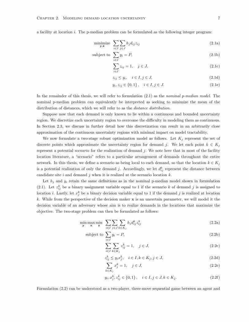
a facility at location i. The p-median problem can be formulated as the following integer program:
minimizey,z
∑i∈I
∑j∈J
hjdijzij (2.1a)
subject to∑i∈I
yi = P, (2.1b)∑i∈I
zij = 1, j ∈ J, (2.1c)
zij ≤ yi, i ∈ I, j ∈ J, (2.1d)
yi, zij ∈ {0, 1} , i ∈ I, j ∈ J. (2.1e)
In the remainder of this thesis, we will refer to formulation (2.1) as the nominal p-median model. The
nominal p-median problem can equivalently be interpreted as seeking to minimize the mean of the
distribution of distances, which we will refer to as the distance distribution.
Suppose now that each demand is only known to lie within a continuous and bounded uncertainty
region. We discretize each uncertainty region to overcome the difficulty in modeling them as continuous.
In Section 2.3, we discuss in further detail how this discretization can result in an arbitrarily close
approximation of the continuous uncertainty regions with minimal impact on model tractability.
We now formulate a two-stage robust optimization model as follows. Let Kj represent the set of
discrete points which approximate the uncertainty region for demand j. We let each point k ∈ Kj
represent a potential scenario for the realization of demand j. We note here that in most of the facility
location literature, a “scenario” refers to a particular arrangement of demands throughout the entire
network. In this thesis, we define a scenario as being local to each demand, so that the location k ∈ Kj
is a potential realization of only the demand j. Accordingly, we let dkij represent the distance between
candidate site i and demand j when it is realized at the scenario location k.
Let hj and yi retain the same definitions as in the nominal p-median model shown in formulation
(2.1). Let zkij be a binary assignment variable equal to 1 if the scenario k of demand j is assigned to
location i. Lastly, let xkj be a binary decision variable equal to 1 if the demand j is realized at location
k. While from the perspective of the decision maker x is an uncertain parameter, we will model it the
decision variable of an adversary whose aim is to realize demands in the locations that maximize the
objective. The two-stage problem can then be formulated as follows:
miny
maxx
minz
∑i∈I
∑j∈J
∑k∈Kj
hjdkijz
kij (2.2a)
subject to∑i∈I
yi = P, (2.2b)∑i∈I
∑k∈Kj
zkij = 1, j ∈ J, (2.2c)
zkij ≤ yixkj , i ∈ I, k ∈ Kj , j ∈ J, (2.2d)∑k∈Kj
xkj = 1, j ∈ J, (2.2e)
yi, xkj , z
kij ∈ {0, 1} , i ∈ I, j ∈ J, k ∈ Kj . (2.2f)
Formulation (2.2) can be understood as a two-player, three-move sequential game between an agent and

Chapter 2. Modeling demand location uncertainty 8
Figure 2.1: Example of a three-move game with one demand (1 - facility placement by agent, 2 - demandrealization by adversary, 3 - demand assignment by agent)
an adversary (nature). In the first move, an agent decides on a set of facility locations, based only
on knowledge of the uncertainty regions of each demand and the corresponding demand weights. In
the second move, the adversary realizes each demand at a location within its respective uncertainty
region. In the third move, having now observed the realized demand locations, the agent then assigns
the demands to facilities. The equilibrium that results from this game represents the optimal solution
to (2.2). Figure 2.1 shows a simple example of one of these games.
This model belongs to a class of games known as Stackelberg games, wherein an agent must commit
to a strategy prior to the adversary, allowing the adversary to observe the agent’s decisions and respond
accordingly (Paruchuri et al., 2008; Brown et al., 2006, 2009). Within the optimization framework, these
games typically take on a min-max-min structure, where each operator represents a move in the game.
Brown et al. (2006) simplify a min-max-min formulation by replacing the inner minimization problem
with its dual equivalent, resulting in a simpler min-max optimization problem. Applying this approach
to (2.2) yields a bilinear objective in the equivalent min-max problem as a result of constraint (2.2e).
To avoid the bilinearity, we instead present a reformulation which allows us to obtain an equivalent
min-max problem with a linear objective. This reformulated problem then lends itself to several solution
approaches that we discuss in Chapter 3.
First, we modify constraint (2.2c) by removing the inner sum over all k ∈ Kj and enforcing the
constraint over all k ∈ Kj and all j ∈ J . Intuitively, this modified constraint forces every scenario of
every demand to be assigned to a facility, instead of only assigning the scenarios which host a realized
demand. The xkj term is then dropped from constraint set (2d) to maintain feasibility. To ensure that
each demand-facility pairwise distance only contributes to the objective function once, we introduce
xkj to the objective. This ensures that only the distance between the realized demand location and its

Chapter 2. Modeling demand location uncertainty 9
nearest facility is counted. These changes yield the following problem:
miny
maxx
minz
∑i∈I
∑j∈J
∑k∈Kj
hjdkijz
kijx
kj (2.3a)
subject to∑i∈I
yi = P, (2.3b)∑i∈I
zkij = 1, k ∈ Kj , j ∈ J, (2.3c)
zkij ≤ yi, i ∈ I, k ∈ Kj , j ∈ J, (2.3d)∑k∈Kj
xkj = 1, j ∈ J, (2.3e)
yi, xkj , z
kij ∈ {0, 1} , i ∈ I, k ∈ Kj , j ∈ J. (2.3f)
Lemma 1 The optimal values of (2.2) and (2.3) are equal.
We now make two additional observations which allow us to further simplify (2.3).
Lemma 2 For a feasible y, the inner max-min problem in (2.3) contains a saddle point.
First, we note that as a result of the reformulation, the two-move game represented by the inner
max-min problem in (2.3) now contains a saddle point. This allows the order of the max and inner min
operators to be exchanged without affecting the optima. In a game-theoretic context, this implies that
agent now gains no useful information from the observation of the demand locations x, since each scenario
of each demand can be optimally “pre-assigned” to its nearest facility. This reduces the Stackelberg game
to two-moves, as the facility placement and demand assignment decisions can now both be made in the
first move.
Lemma 3 For a feasible y, the optimal value of (2.3) remains unchanged when the integrality constraints
on x and z are relaxed.
Second, we observe that the integrality constraints on x and z can both be relaxed without changing
the optima. As will be shown in Section 3.2, relaxing x to be a continuous variable allows us to exploit
linear programming duality to obtain an exact duality-based reformulation. This relaxation also greatly
reduces the number of binary variables in the model.

Chapter 2. Modeling demand location uncertainty 10
These two observations allows us to obtain our final formulation for the robust p-median model:
miny,z
maxx
∑i∈I
∑j∈J
∑k∈Kj
hjdkijx
kj zkij (2.4a)
subject to∑i∈I
yi = P (2.4b)∑i∈I
zkij = 1, k ∈ Kj , j ∈ J, (2.4c)
zkij ≤ yi, i ∈ I, k ∈ Kj , j ∈ J, (2.4d)∑k∈Kj
xkj = 1, j ∈ J, (2.4e)
yi ∈ {0, 1} , i ∈ I, (2.4f)
xkj , zkij ≥ 0, i ∈ I, k ∈ Kj , j ∈ J. (2.4g)
For conciseness, in the remainder of the thesis we let
X =
xkj ≥ 0
∣∣∣∣ ∑k∈Kj
xkj = 1, ∀j ∈ J
,
Y =
{yi ∈ {0, 1}
∣∣∣∣ ∑i∈I
yi = P
},
and Z(y) =
zkij ≥ 0
∣∣∣∣ ∑i∈I
∑k∈Kj
zkij = 1,∀j ∈ J ; zkij ≤ yi, ∀i ∈ I, k ∈ Kj , j ∈ J
.
Clearly, the uncertainty in demand locations also introduces uncertainty in the distance between each
demand and its nearest facility. As a consequence, we no longer obtain a single distance distribution
for a given set of facilities, but are instead presented with a family of distributions. Similarly, the mean
(weighted) distance, which can be calculated if all demand locations are known, is now replaced with
an interval for the true mean. Thus, just as the nominal p-median minimizes the mean of the distance
distribution, the robust p-median model seeks to minimize the worst-case mean, i.e. the upper endpoint
of the interval in which the true mean lies.
2.1.2 P-center problem
The classical p-center problem seeks to locate p facilities in a network such that some maximum cost
over a set of demands is minimized, typically the weighted distance of the demand to its nearest facility
(Tansel et al., 1983). Using the same notation and constraint set as the nominal p-median formulation
(2.1), the nominal p-center problem can be formulated as follows:
minimizey,z
{maxj∈J
{∑i∈I
hjdijzij
}}(2.5a)
(2.1b)− (2.1e).

Chapter 2. Modeling demand location uncertainty 11
By introducing discrete uncertainty regions for each demand using the same framework as in formulation
(2.4), we obtain the following robust optimization model:
miny,z
maxx
maxj∈J
{∑i∈I
∑k∈Kj
hjdkijz
kijx
kj
} (2.6a)
x ∈ X, z ∈ Z(y), y ∈ Y. (2.6b)
We note that the feasible set X can be separated in j such that X =∏j∈J
Xj , where
Xj =
xkj∣∣∣∣ ∑k∈Kj
xkj = 1
.
This implies that for a feasible z,
maxx
maxj∈J
{∑i∈I
∑k∈Kj
hjdkij z
kijx
kj
} = maxj∈J
maxxj
{∑i∈I
∑k∈Kj
hjdkij z
kijx
kj
}Using this result and a dummy variable t, we can reformulate (2.6) to obtain our final robust p-center
problem:
minimizey,z,t
t (2.7a)
subject to t ≥ maxx
∑i∈I
∑k∈Kj
hjdkijz
kijx
kj , j ∈ J, (2.7b)
x ∈ X, z ∈ Z(y), y ∈ Y. (2.7c)
Whereas the nominal p-center model minimizes the maximum value in the distance distribution, the
robust p-center model similarly seeks to minimize the maximum value within the worst-case distance
distribution.
2.1.3 Conditional value-at-risk
Conditional value-at-risk (CVaR) is a coherent risk measure with origins in the mathematical finance
literature and is based on the related value-at-risk (VaR) measure (Rockafellar and Uryasev, 2000).
Briefly, suppose f(y, ξ) is a loss (or cost) function that depends on a decision variable y and a random
vector ξ, with density p(ξ) assumed to exist. Given a risk tolerance 1− β (where β is commonly 0.95 or
0.99), the value-at-risk is the lowest threshold α such that the probability of f(y, ξ) exceeding α is exactly
1− β. Then, β-CVaR is the expected loss conditional on the loss exceeding α. In other words, it is the
average value of the outcomes at or above the βth percentile of the distribution. CVaR’s popularity in
the optimization literature stems from its tractability. Additionally, since by definition CVaR is always
greater than VaR, minimizing CVaR offers a tractable way of limiting VaR as well. In general, CVaR
can be minimized by (Rockafellar and Uryasev, 2000):
minimizey, α
α+1
1− β
∫f(y,ξ)≥α
(f(y, ξ)− α)p(ξ)dξ (2.8)

Chapter 2. Modeling demand location uncertainty 12
The corresponding value of VaR is simply the optimal α in (2.8). Further, if the continuous density
p(ξ) is replaced with a discrete distribution, the problem reduces to a linear program. Suppose Ξ =
{ξ1, ξ2, ..., ξ|S|} is the set of possible outcomes of a discrete random variable, which occur with probability
p(ξs) = ps. The minimization of CVaR can then be modelled as the following linear program:
minimizey, α
α+1
1− β∑s∈S
ps max {f(y, ξs)− α, 0} (2.9)
We now consider a CVaR-based location problem with deterministic demand locations. Let us use
the same variable and parameter definitions and constraint set as in (2.1). Let the loss function be
fj(zj) =∑i∈I dijzij , which is the distance between a demand and its assigned facility. In this model,
we let each demand j be analogous to an event s from (2.9). Similarly, in place of the event probability
ps, we use the demand weight hj , which can be normalized so that∑j∈J hj = 1. Then, we can minimize
the average distance at the tail of the distance distribution – where the tail is defined as all distances at
or above 100βth percentile – by solving the following nominal CVaR problem:
minimizey,z
α+1
1− β∑j∈J
hj max {fj(zj)− α, 0} (2.10a)
subject to (2.1b)− (2.1e).
We include demand weight parameter hj to generalize the model, so that some demands can be em-
phasized more than others. Suppose now that the demand locations are uncertain, where xj represents
the true location of demand j. Let the loss function for a single demand j again be the distance to its
assigned facility. However, the distance to its assigned facility is now also a function of xj :
fj(xj , zj) =∑i∈I
∑k∈Kj
dkijzkijx
kj
The uncertainty in demand locations means that CVaR cannot be directly evaluated. However, given
a set of facilities and assignment decisions, we can evaluate the worst-case CVaR as follows:
maxx
minα
α+1
1− β∑j∈J
hj max {fj(xj , zj)− α, 0} (2.11)
We can minimize the worst-case CVaR with the following model:
miny,z
maxx
minα
α+1
1− β∑j∈J
hj max {fj(xj , zj)− α, 0} (2.12a)
subject to x ∈ X, z ∈ Z(y), y ∈ Y. (2.12b)
Finally, we provide a reformulation of (2.12) which simplifies it from a two-stage model to a min-max

Chapter 2. Modeling demand location uncertainty 13
formulation:
minimizey,z,α
α+1
1− β∑j∈J
hjγj (2.13a)
subject to γj ≥ maxx
fj(xj , zj)− α, ∀j ∈ J, (2.13b)
x ∈ X, z ∈ Z(y), y ∈ Y. (2.13c)
Lemma 4 The optimal values of (2.12) and (2.13) are equal.
We envision coherent risk measures such as CVaR as being useful metrics in healthcare operations, where
there is an interest in hedging against risk. Additionally, these measures may be useful in guiding decision
making in contexts where fairness and equity play a significant role. For example, in ambulance location
problems, an expected distance minimization scheme might not be appropriate if a low-weighted area
receives extremely poor service. Further, as mentioned earlier, risk-based targets are already present in
emergency medicine. CVaR-based location models may therefore be useful in assisting health service
planners in meeting these standards.
We note here that Chen et al. (2006) also develop a scenario-based facility location model with a
CVaR objective, which they refer to as the mean-excess regret model. Their model takes a stochastic
approach by assuming the probability of each potential demand realization is known. Our model differs
in that our uncertainty is in the location of each individual demand, and we use no distributional
information.
2.2 Relationship of p-median and p-center to CVaR
The CVaR models (both nominal and robust) can be viewed as a compromise between the p-median
and p-center models, in that they focus on optimizing the tail of the distribution, as opposed to the
mean or the absolute maximum. In fact, we can show that both the p-median and p-center problems
are special cases of the CVaR model, depending on how β is chosen. This result implies that, on its
own, the robust CVaR model provides a highly general framework for shaping the distance distribution,
and allows the decision maker to optimize the mean, maximum, or tail average by simply choosing an
appropriate value for β.
Specifically, we show that for a β value of 0, the CVaR model specializes to the p-median, and for
β values that are sufficiently close to 1, the CVaR model specializes to the p-center. As a result, by
adjusting the β parameter from 0 to 1, we can “sweep out” a spectrum of models between the p-median
and the p-center problem.
Proposition 1 Let ZV and ZM be the optimal values of the robust CVaR and the robust p-median
models, respectively. If β = 0, then ZV = ZM .
Proof: Let (α∗,x∗,y∗, z∗) be an optimal solution to the robust CVaR model as shown in formulation
(2.12). The optimal value is then given by
ZV = α∗ +1
1− β∑j∈J
hj max{fj(x
∗j , z∗j )− α∗, 0
}

Chapter 2. Modeling demand location uncertainty 14
We observe that with β = 0, if fj(xj , zj) − α∗ ≥ 0 for all j, then the CVaR objective reduces to the
p-median objective:
ZV = α∗ +1
1− β∑j∈J
hj[fj(x
∗j , z∗j )− α∗
]= α∗ +
∑j∈J
hjfj(x∗j , z∗j )−
∑j∈J
hjα∗
= α∗(
1−∑j∈J
hj
)+∑j∈J
hjfj(x∗j , z∗j )
=∑j∈J
hjfj(x∗j , z∗j )
=∑i∈I
∑j∈J
∑k∈Kj
hjdkijz
k∗ij x
k∗j
Formulations (2.4) and (2.12) show that the feasible regions of y, x and z are identical in both the p-
median and CVaR models. Since the objective functions are also the same if fj(x∗j , z∗j )−α∗ ≥ 0, ∀j ∈ J ,
then (x∗,y∗, z∗) must also be an optimal solution to the robust p-median model, which gives us ZV = ZM .
We are now required to show that fj(x∗j , z∗j )− α∗ ≥ 0 in all cases where β = 0. This is clearly true
in the case where α∗ = 0, since fj(x∗j , z∗j ) is always positive for all j ∈ J .
For α∗ > 0, suppose by contradiction that there exists some j such that fj(x∗j , z∗j ) − α∗ < 0. Now
suppose we replace α∗ with (α∗ − δ) ≥ 0. The new objective value is given by:
ZnewV = (α∗ − δ) +∑j∈J
hj max{fj(x
∗j , z∗j )− (α∗ − δ), 0
}< (α∗ − δ) +
∑j∈J
hj max{fj(x
∗j , z∗j )− α∗, 0
}+∑j∈J
hjδ
< α∗ +∑j∈J
hj max{fj(x
∗j , z∗j )− α∗, 0
}+
∑j∈J
hj − 1
δ
< ZV +
∑j∈J
hj − 1
δ
< ZV
But ZnewV < ZV contradicts the optimality of ZV , so fj(x∗j , z∗j )− α∗ ≥ 0 for all j ∈ J . �
Proposition 2 Let ZV and ZT be the optimal values of the robust CVaR and the robust p-center models,
respectively. If β is arbitrarily close to 1, then ZV = ZT .
Proof: Let (α∗,x∗,y∗, z∗) be an optimal solution to the robust CVaR model. Note that if α∗ =

Chapter 2. Modeling demand location uncertainty 15
maxj∈J{fj(x∗j , z∗j )}, then the robust CVaR objective reduces to the robust p-center objective:
ZV = α∗ +1
1− β∑j∈J
hj max{fj(x
∗j , z∗j )− α∗, 0
}= max
j∈J{fj(x∗j , z∗j )}+
1
1− β∑j∈J
hj max
{fj(x
∗j , z∗j )−max
j∈J{fj(x∗j , z∗j )}, 0
}= max
j∈J{fj(x∗j , z∗j )}
Since the feasible regions in the robust p-center and robust CVaR models are the same, this implies that
(x∗,y∗, z∗) is also an optimal solution to the p-center problem, which gives us ZV = ZT . It remains to
show that α∗ = maxj∈J{fj(x∗j , z∗j )} in all cases where β is arbitrarily close to 1.
We now show that neither α∗ > maxj∈J{fj(x∗j , z∗j )} nor α∗ < max
j∈J{fj(x∗j , z∗j )} can hold at optimality.
For the first inequality, we can find a δ > 0 such that max{fj(x
∗j , z∗j )− (α∗ − δ), 0
}= 0 for all j ∈ J .
This suggests that we could obtain a new objective value:
ZnewV = α∗ − δ +1
1− β∑j∈J
hj max{fj(x
∗j , z∗j )− (α∗ − δ), 0
}= ZV − δ
< ZV
This contradicts the optimality of ZV , so α∗ > maxj∈J{fj(x∗j , z∗j )} cannot hold. For the second inequality,
suppose α∗ < maxj∈J
{fj(x∗j , z∗j )}. This implies there exists some j ∈ J such that maxj∈J
{fj(x∗j , z∗j ) −
α∗ , 0} > 0. But then we obtain
α∗ + limβ→1
1
1− β∑j∈J
hj max{fj(x∗j , z∗j )− α∗ , 0} =∞ > maxj∈J{fj(x∗j , z∗j )}
This implies that as β gets close to 1, any solution where α∗ < maxj∈J
{fj(x∗j , z∗j )} will clearly be sub-
optimal. This completes the proof. �
The relationship between CVaR and the p-median and p-center models is intuitive when we recall that
β-CVaR is defined as the mean loss of all demands at or above the 100βth percentile of the distribution.
Thus when β is zero, the β-CVaR is the mean of the distribution itself. Similarly, when β is arbitrarily
close to 1, the β-CVaR is the loss of the demand at the extreme upper-tail of the distance distribution,
which is the demand that is furthest from any facility.
2.3 Bounds on the discrete approximation error
The discretization of the uncertainty regions introduces an error in the evaluation of the worst-case total
distance for a set of facilities, since the possible locations where demands may be realized are constrained
to a finite subset of points within the continuous uncertainty region. In this section, we present a bound
on the error introduced by the discretization, which then allows us to bound the true worst-case distance
to the nearest facility for a given demand. This then allows us to construct bounds on the theoretical

Chapter 2. Modeling demand location uncertainty 16
worst-case distance objective of the corresponding continuous problem for each of the three location
models.
Consider an arbitrary demand j. Suppose a set of facilities is fixed. Let Uj be the continuous
uncertainty region around j, and let Qj = {q1,q2, ...,q|Kj |} be the set of points representing the discrete
scenarios for the realization of demand j. Let R be the set of facility locations and let dj(·, ·) measure
the Euclidean distance between any two points in demand region j. Next, we define the parameter
`j = maxp∈Uj
minq∈Qj
dj(p,qk), which is the maximum distance between any point p ∈ Uj and its closest
discrete scenario location qk. Let qd be the location which represents the worst-case realization of
demand j within the discrete uncertainty region, and let rd be the nearest facility to qd. Similarly, let
pc be the location of the worst-case realization assuming a continuous uncertainty region, and let rc the
facility nearest to pc.
Lemma 5 For an arbitrary demand j, 0 ≤ dj(pc, rc)− dj(qd, rd) ≤ `j .
Proof: Consider the first inequality. First, the worst-case distance assuming a continuous uncertainty
region must be at least as large as the worst-case distance when the demand is constrained to be realized
at one of the |Kj | scenarios. This yields dj(qd, rd) ≤ dj(pc, rc), and thus 0 ≤ dj(pc, rc)− dj(qd, rd).
For the second inequality, let qf ∈ Uj be the nearest discrete demand scenario to pc. We first show
that dj(pc, rc)−dj(qf , rf ) ≤ `j . The triangle inequality implies dj(p
c, rf )−dj(qf , rf ) ≤ dj(pc,qf ). By
definition of `j , dj(pc,qf ) ≤ `j , so dj(p
c, rf )− dj(qf , rf ) ≤ `j . Also by definition, since rc is the closest
facility to pc, dj(pc, rc) ≤ dj(p
c, rf ), which implies dj(pc, rc) − dj(qf , rf ) ≤ `j . Lastly, since qd is the
worst-case discrete location, the distance to its nearest facility must be at least as large as dj(qf , rf ).
This gives us dj(qf , rf ) ≤ dj(qd, rd), which implies dj(p
c, rc)− dj(qd, rd) ≤ dj(pc, rc)− dj(qf , rf ) ≤ `j .�
We note that the problem of determining `j for the discrete uncertainty set Qj is related to the largest
empty circle problem (Toussaint, 1983). Given a finite set of points P in a plane, the largest empty circle
problem asks how large a circle can be constructed such that its center lies within the convex hull of
P and no point in P lies within the circle. Similarly, the calculation of `j is equivalent to the radius
of the largest circle possible such that its center lies within Uj and no point from Qj lies within the
circle’s interior. However, calculating `j can be challenging, especially if each of the uncertainty regions
assumes a different form. Alternatively, we make two assumptions which allow us to quantify an upper
bound on `j .
Assumption 1 The discrete set Qj takes the form of a square lattice over the region Uj with a grid
spacing of length s.
Assumption 2 Suppose S is a set of discrete points which creates a square lattice over the entire plane
such that Qj ⊂ S, ∀j ∈ J . The shape of the uncertainty region Uj is such that for any point p ∈ Uj,
at least one of the four points in S which define the smallest square around p is inside Uj.
Assumption 1 is a modeling decision that can be satisfied easily. Assumption 2 excludes pathologically
shaped uncertainty regions which make it difficult to bound the discretization error. With this, we present
a bound on the error introduced by the discretization of the uncertainty regions. Let the dicretization
error, ∆med, be defined as follows:
∆med =ZC − ZD
ZC

Chapter 2. Modeling demand location uncertainty 17
where ZD represents the optimal value from solving (2.4) and ZC represents the theoretical optimal value
from solving the same problem assuming continuous uncertainty regions. Similarly, let ZN represent the
optimal value of the associated nominal problem (where the uncertainty region is a singleton for each
demand).
Theorem 1 For any ε > 0, if s ≤ εZN√2∑
j hj, then ∆med ≤ ε.
Proof: Assumptions 1 and 2 imply `j ≤√
2s. Thus, dj(pc, rc)− dj(qd, rd) ≤
√2s, and
ZC − ZD =∑j∈J
hjdj(pc, rc)−
∑j∈J
hjdj(qd, rd)
≤√
2s∑j∈J
hj
Dividing both sides by ZC ,
∆CD =ZC − ZD
ZC≤√
2s∑j hj
ZC
Lastly, since ZN ≤ ZD ≤ ZC , we obtain
∆CD ≤√
2s∑j hj
ZC≤√
2s∑j hj
ZD≤√
2s∑j hj
ZN= ε. �
If ZN is known, then by Theorem 1 an upper bound on the discretization error can be expressed in
closed form as a function of the discrete spacing s. As a result, this allows us to determine how finely the
uncertainty regions must be discretized such that the discretization error ∆med is no greater than some
target value, without having to first solve the robust problem. Alternatively, since ZD ≥ ZN , the robust
problem itself could be solved to obtain ZD, which leads to a tighter bound through the substitution of
ZN with ZD in Theorem 1.
The bound can be further tightened by enforcing a slightly stronger condition on the shape of the
uncertain regions. If we modify Assumption 2 so that three of the four points in a square lattice S which
define the smallest square around any point p ∈ Uj are within Uj , then `j can be bounded by s instead
of√
2s. For example, this stronger assumption is satisfied by circular uncertainty regions.
To examine how the bound improves as a function of s, we construct a test problem with 50 candidate
sites, 10 equally-weighted demands and 5 facilities. Each uncertainty region is modeled as a circle with a
radius of 50, and discretized with a square lattice. The problem is solved for values of s ranging from 50
to 0.1, corresponding to a range of 5 to 820,000 scenarios per demand, respectively (we use an efficient
solution method developed in Chapter 3 to solve all problem instances). The results are shown in Figure
2.2. The two upper bounds on ZC shown in Figure 2.2 are calculated using Theorem 1 as follows:
ZCN=
ZD1− εN
, where εN =
√2s∑j hj
ZN
ZCD=
ZD1− εD
, where εD =
√2s∑j hj
ZD
Figure 2.2 shows how the solution to the robust formulation (2.4) serves as a lower bound on ZC .

Chapter 2. Modeling demand location uncertainty 18
101
102
103
104
105
2100
2150
2200
2250
2300
2350
2400
Tot
al D
ista
nce
scenarios / demand
ZCN
ZCD
ZD
101
102
103
104
105
10−3
10−2
10−1
100
scenarios / demand
Err
or b
ound
, ε
εNεD
Figure 2.2: Bound on continuous worst-case distance ZC (top); bound on discretization error, ∆med
(bottom)
The results show that the error bound may be weak if the uncertainty regions are discretized with
only a small number of scenarios. However, in Section 3.3 we show that the uncertainty regions can be
discretized finely to obtain tight bounds on ZC without sacrificing model tractability.
We can also develop a similar bound on the discretization error for the robust p-center problem,
∆cen.We redefine ZC and ZD to be the optimal value of the robust p-center problem assuming continuous
and discrete uncertainty regions, respectively, and ZN to be the optimal value of the nominal problem.
We assume that Assumptions 1 and 2 hold here as well.
Theorem 2 For any ε > 0, if s ≤ εZN√2max
j∈J{hj}
, then ∆cen ≤ ε.
Proof: For conciseness we let
fj(xj , zj) =∑i∈I
∑k∈Kj
dkijzkijx
kj
Now let (y∗, z∗,x∗) be the optimal solution to (2.6). By Lemma 5, an upper bound on the true worst-case
distance for a demand j for the given solution is
dj(qd, rd) +
√2s = fj(x
∗j , z∗j ) +
√2s.

Chapter 2. Modeling demand location uncertainty 19
The absolute gap between the optimal values of (2.6) and the corresponding continuous problem can
thus be bounded as follows:
ZC − ZD ≤ maxj∈J
{hj
(fj(xj , zj) +
√2s)}− ZD
≤ maxj∈J{hjfj(xj , zj)}+ max
j∈J{hj√
2s} − ZD
=√
2s maxj∈J{hj} .
Then the relative gap in the robust p-center model can be bounded by
∆cen :=ZC − ZD
ZC≤
√2s max
j∈J{hj}
ZN= ε. �
Lastly, we can again use Lemma 5 to provide a bound for the robust CVaR model. As before, let
the optimal value of the robust CVaR model shown in (2.13) be ZD, and let the optimal value of the
associated continuous uncertainty problem be ZC .
Theorem 3 For any ε > 0, if√
2s ≤ ε(1−β)ZN∑j hj
, then ∆CV aR ≤ ε.
Proof: Suppose (y∗, z∗,x∗, α∗) is the optimal solution to (2.13). Let gj(xj , zj) be the loss function for
a demand j assuming a continuous uncertainty region. Lemma 5 implies gj(x∗j , z∗j ) ≤ fj(x
∗j , z∗j ) + s. A
bound on the absolute gap between ZC and ZD can therefore be given by:
ZC − ZD ≤ α∗ +1
1− β∑j∈J
hj max{gj(x
∗j , z∗j )− α∗, 0
}− ZD
≤ α∗ +1
1− β∑j∈J
hj max{fj(x
∗j , z∗j ) +
√2s− α∗, 0
}− ZD
≤ α+1
1− β∑j∈J
hj[
max{fj(x
∗j , z∗j )− α∗, 0
}+√
2s]− ZD
=1
1− β∑j∈J
hj√
2s.
Letting ZN be the optimal value of the nominal problem, we can bound the discretization error by
∆CV aR :=ZC − ZD
ZC≤ 1
(1− β)ZN
∑j∈J
hj√
2s = ε. �
As in the previous two models, we do not need to actually solve (2.13) in order to develop a bound on
the relative error ∆CV aR, since only ZN is required.
These bounds show that while a continuous uncertainty region may be more representative of the
actual uncertainty in demand locations, our discrete approach can still provide a good approximation
if the discrete grid size is selected appropriately. In particular, Figure 2.2 shows the grid size necessary
to reach a certain discretization error. As a result, instead of solving a robust optimization problem
with continuous uncertainty regions, which can be difficult, we can solve the discretized formulations
and then provide an upper bound on the true worst-case objective function, ZC .

Chapter 2. Modeling demand location uncertainty 20
2.4 A continuous demand interpretation
In practice, demands may not be concentrated at a finite set of nodes, but are instead likely to exist
continuously in the plane. For example, the demand for an ambulance may realistically emanate from any
location in an urban area. As a result, it may be beneficial to view demand as a continuous distribution
rather than existing at a set of nodes. In this section we show how an alternate interpretation of our
robust optimization models allows us to model continuous demand in settings where there is uncertainty
in the spatial distribution.
One possible approach to modeling continuous demand is to uniformly discretize the continuous
space with a very large number of discrete nodes, and to assign a demand weight to each of these nodes.
However, there are limitations to this approach. First, this may lead to an intractable formulation due to
the extremely large number of demand nodes that would be required to reasonably discretize the plane.
Second, even in the absence of computational challenges, it may be difficult to accurately estimate an
appropriate weight for each of these demand nodes. To illustrate, consider again the problem of siting
emergency services facilities in an urban area. Suppose we discretize the continuous demand in space
into an extremely large number of discrete points S, such that each point s represents an individual
building in the city, and the node weight ps represents the probability that a random future emergency
will occur in building s (alternatively, each s could represent an arbitrarily sized area in the city, such
as a single city block, depending on how finely we discretize the continuous demand). We can then
minimize the expected distance between a future emergency and its nearest facility with a stochastic
interpretation of the p-median model:
minimizey, z
∑i∈I
∑s∈S
psdiszis
In practice, however, it is extremely difficult to predict the future demand for an ambulance at the
individual building or even city block level, meaning any estimate of ps is likely to be highly uncertain.
A more viable approach is to use historical data to forecast the total demand emanating from a geographic
subregion, which would be represented as group of multiple discrete nodes. Letting S again be the set
of all demand points in the plane, suppose we now divide it into subregions indexed by j, so that
S = ∪j∈JKj . We let Kj be indexed by k, so that each index pair (j, k) represents a unique demand
node s.
Suppose now that the aggregate future demand emanating from region j can be accurately predicted,
hj , but that the distribution of demand within region j is uncertain. We can then formulate a problem
which minimizes the worst-case expected distance to a facility:
miny,z
maxp
∑i∈I
∑j∈J
∑k∈Kj
pkj dkijz
kij (2.14a)
subject to∑k∈Kj
pkj = hj , ∀j ∈ J, (2.14b)
z ∈ Z(y), y ∈ Y. (2.14c)
Constraint (2.14b) forces the total demand over subregion j to be equal to hj . Now, since the uncertainty

Chapter 2. Modeling demand location uncertainty 21
is in the distribution within each subregion j, we can write
pkj = hj xkj
where xkj is the uncertain parameter representing the fraction of hj that lies at point k ∈ Kj . This yields
the following problem, which is clearly equivalent to (2.4):
miny,z
maxx
∑i∈I
∑j∈J
∑k∈Kj
hjxkj dkijz
kij (2.15a)
subject to∑k∈Kj
xkj = 1, ∀j ∈ J, (2.15b)
z ∈ Z(y), y ∈ Y. (2.15c)
This interpretation allows us to minimize the worst-case expected distance in problems where the demand
is continuous in space but is subject to distributional uncertainty. In this context, xj represents the
unknown discrete demand distribution over the demand nodes Kj which constitute subregion j. Note
that since we impose no constraints on the demand distribution other than forcing it to sum to 1, the
worst-case distribution over each demand region will always take the form of a delta function at the
point furthest from any facility.
If this uncertainty set for the demand distribution is too conservative, we can add an additional
constraint that forces the share of the probability mass to be no greater than δ for any one location k.
Alternatively, if the nominal location of each demand is included as a scenario (e.g. k = 1), then we
can enforce linear constraints which limit the total number of demands that are allowed to deviate from
their nominal locations.

Chapter 3
Decomposition techniques
In this chapter, we propose a row-and-column generation algorithm that can be used to solve the formu-
lations developed in Chapter 2. Our technique relies on reducing the size of the optimization problem
through the elimination of redundant variables and their associated constraints. For brevity, all solution
approaches discussed in this section are in the context of the robust p-median formulation shown in
(2.4). Our methodology can be extended to the robust p-center and robust CVaR formulations shown
in (2.7) and (2.13), as a result of their similar structure.
In Section 3.1 we review a classic row generation algorithm used for decomposing min-max problems
and compare it with our row-and-column generation algorithm. We will refer to these as the “primal
methods” because the adversary problem retains its primal form in the min-max formulation that is
decomposed. In Section 3.2 we consider an exact duality-based reformulation of (2.4), and then apply
a similar decomposition technique based on row-and-column generation. Similarly, we refer to these
approaches as the “dual methods”, since we take the dual of the adversary problem in both methods.
In Section 3.3 we present results from a short study on the computational performance of these solution
methods.
3.1 Primal methods
Brown et al. (2006, 2009) use a row generation algorithm for solving min-max problems, which they
refer to as Benders-based decomposition. We briefly review this approach and then present our row-
and-column generation algorithm.
3.1.1 Row-generation only
Let the objective function of the robust p-median model be f(x, z). Formulation (2.4) can be reformu-
lated with the use of a dummy variable as follows:
minimizey,z,t
t (3.1a)
subject to t ≥ f(x, z), x ∈ X (3.1b)
z ∈ Z(y), y ∈ Y. (3.1c)
22

Chapter 3. Decomposition techniques 23
Since we allow x to be continuous, this problem cannot be solved as a MIP due to the infinite constraint
set (3.1b). Even in the case where x remains binary, this would still result in a constraint set which
grows exponentially with the number of scenarios per demand (assuming all demands have the same
number of scenarios).
Alternatively, (3.1) can be solved using the following row generation algorithm. First, we solve a
relaxed version of (3.1) by only enforcing the constraint for the subset X = {x1}, where x1 represents the
nominal demand pattern. After obtaining the optimal solution (y∗, z∗, t∗), we identify the corresponding
worst-case demand locations x∗ by solving the inner maximization problem of (2.4). If we obtain a
violating constraint such that t∗ < f(x∗, z∗), then the current solution (y∗, z∗, t∗) cannot be feasible
for all x ∈ X, and is therefore cannot be an optimal solution to (3.1). Then, we add the constraint
t ≤ f(x∗, z∗) to (3.1) and re-solve it to obtain a new optimal set of facility locations. When no more
violating constraints can be identified, the current solution is optimal.
Let us describe the approach formally. Let S be an index set for the iterations of the algorithm,
and let the optimal solution of the subproblem on the sth iteration of the algorithm be xs. Thus X
is updated with each iteration with X ← X ∪ xs. The set S also serves to index all of the “demand
patterns” in X.
The master and subproblem for the row generation algorithm can be written as follows:
(Master problem)
minimizey,z,t
t (3.2a)
subject to t ≥∑i∈I
∑j∈J
∑k∈Kj
zkijdkijh
kj x
ksj , s ∈ S, (3.2b)
z ∈ Z(y), y ∈ Y. (3.2c)
(Sub-problem)
maximizex
∑i∈I
∑j∈J
∑k∈Kj
zkijdkijh
kjx
kj (3.3a)
subject to x ∈ X. (3.3b)
An alternate stopping criterion is to terminate the algorithm once the optimal values of the master and
subproblem converge to within some desired tolerance. This is the approach used in Brown et al. (2006).
As a result of the structure of X, subproblem (3.3) can be solved in closed form as follows. Let I1 ∈ Ibe the set where I1 = {i|yi = 1}. Then for each demand j, we set xk
∗
j = 1 where
k∗ = arg maxk∈Kj
{mini∈I1
{dkijhj
}}Instead of solving the subproblem as a linear program, we can use a simple sorting algorithm based on
the rule above. The computational performance of the algorithm is therefore determined primarily by
the solution of the master problem, because the sorting algorithm is extremely fast even for large lists.

Chapter 3. Decomposition techniques 24
3.1.2 Row and column generation
Our method improves upon the approach in Section 3.1.1 by eliminating variables and constraints from
the master problem that we identify as redundant. We consider a constraint redundant if removing the
constraint and then resolving the master problem results in no change in the optimal solution. Similarly,
we consider a variable redundant if the objective function of the master problem is independent of the
variable’s value. Letting each demand contain K scenarios, the total number of variables in the master
problem of the row-generation approach is given by m(1 + nK). This remains unchanged with each
iteration, since only new constraints are generated throughout the algorithm. However, many of these
variables are redundant and also lead to redundant (non-binding) constraints in the master problem.
Consider the cut generated by the subproblem in the first iteration (s = 1). This constraint is:
t ≥∑i∈I
∑j∈J
∑k∈Kj
hjdkijz
kij x
k1j
This constraint can also be written as
t ≥∑i∈I
∑j∈J
(d1ijz
1ij x
11j + hjd
2ijz
2ij x
21j + ...+ hjd
Kij z
Kij x
K1j
)(3.4)
Now consider an arbitrary demand j. If there exists some k ∈ Kj such that xk1j = 0, then the contribution
of the term hjdkijz
kij x
k1j to the right hand side of the constraint is zero. As a result, the value of the
assignment variable zkij in that term is always multiplied by zero and thus has no impact on the objective
function.
Further, since we know xkj is 1 for exactly one of the K scenarios, this implies that for each (i, j), all
but one of the terms on the right hand side of (3.4) are zero, meaning K − 1 decision variables within
z are redundant. Thus in the first iteration of the row generation algorithm, for every demand j there
are (K − 1)m extraneous variables in the master problem, each of which incurs a redundant constraint
as well (zkij ≤ yi). In the first iteration, there are also an additional (K − 1)n redundant constraints, as
a result of the constraint∑i zkij = 1.
From an intuitive perspective, the extraneous variables are the components of z that are used to
assign the scenarios where the demand is never realized during the algorithm. The master problem in
our row-and-column generation algorithm is able to remain limited in size by creating the zkij assignment
variables and associated dkij parameters in the master problem only when they have been identified as
corresponding to the worst-case demand realization (for that iteration). Since our method relies on
introducing decision variables on an as-needed basis, this incorporates an aspect of column generation
that is not present in the algorithm from Section 3.1.1.
Let us describe the modified master problem formally. Let Ksj = {k|xksj = 1}, so that Ks
j represents
the scenario k for demand j that is realized at iteration s of the algorithm. The master problem for the

Chapter 3. Decomposition techniques 25
row-column generation algorithm can then be written as
minimizey,z,t
t (3.5a)
subject to t ≥∑i∈I
∑j∈J
∑k∈Ks
j
hjdkijz
kij x
ksj , s ∈ S, (3.5b)
∑i∈I
zkij = 1, k ∈ Ksj , j ∈ J, s ∈ S, (3.5c)
zkij ≤ yi, i ∈ I, k ∈ Ksj , j ∈ J, s ∈ S, (3.5d)
y ∈ Y. (3.5e)
The subproblem in this algorithm is the same as in the row-generation algorithm. Now, if at the sth
iteration we let dsij = dkij , ∀i ∈ I, j ∈ J , where k = {k|xkj = 1}, the master problem can be reformulated
as:
minimizey,z,t
t (3.6a)
subject to t ≥∑i∈I
∑j∈J
zsijdsijhj , s ∈ S, (3.6b)
∑i∈I
zsij = 1, j ∈ J, s ∈ S, (3.6c)
zsij ≤ yi, i ∈ I, j ∈ J, s ∈ S, (3.6d)
y ∈ Y. (3.6e)
This equivalent formulation shows that the complexity of the master problem is independent of the
number of scenarios enumerated for each demand.
3.2 Dual methods
In this section we briefly consider a duality based reformulation of (2.4) and show how a row-and-column
generation algorithm can be applied to it as well using a similar argument as in Section 3.1.2.
3.2.1 Equivalent dual formulation
The relaxation of the binary constraint on x transforms the inner maximization problem of (2.4) into a
linear program. This allows us to exploit strong duality to obtain an equivalent problem:
minimizey,z,w
∑j∈J
wj (3.7a)
subject to∑i∈I
hjdkijz
kij − wj ≤ 0, j ∈ J, k ∈ Kj , (3.7b)
z ∈ Z(y), y ∈ Y, (3.7c)
w free. (3.7d)

Chapter 3. Decomposition techniques 26
This formulation can then be solved as a single-stage mixed-integer program. A drawback of this ap-
proach is that adding an additional scenario to each demand increases the number of variables and
constraints by mn and (m + 1)n, respectively. As a result, (3.7) becomes intractable if a large num-
ber of scenarios are used to discretize the uncertainty regions. However, formulation (3.7) may be an
appropriate way of solving smaller instances of (2.4).
3.2.2 Dual master problem with row-and-column generation
Formulation (3.7) can be decomposed and solved using a row-and-column generation technique similar
to the approach discussed in Section 3.1.2. For a fixed y, it is clear that the optimal w∗ in (3.7) is given
by:
w∗j = maxk∈Kj
{mini∈I
{hjd
kij
}}where I =
{i | yi = 1
}. Thus only the constraints that correspond to the worst-case location of each
demand will be binding at optimality. Similarly, the variable zkij for the non-binding constraints will
have no impact on the objective function, and can be removed. This allows us to eliminate extraneous
variables and redundant constraints from the dual problem to obtain a smaller master problem. Then
for a given master problem solution (y∗, z∗), the subproblem from (3.3) can be solved to identify the
worst-case locations, which are used to generate the relevant variables and constraints. The master
problem for the duality-based decomposition is:
minimizey,z,w
∑j∈J
wj (3.8a)
subject to∑i∈I
hjdsijz
sij − wj ≤ 0, j ∈ J, s ∈ S, (3.8b)
z ∈ Z(y), y ∈ Y, (3.8c)
w free. (3.8d)
Comparing the duality-based master problem in formulation (3.8) with the original master problem
in (3.6), we see that the duality-based method we add n cuts at each iteration, one for each wj (constraint
set 3.8b). In the primal method however, we only add one cut on t at each iteration (constraint set
3.6b).
3.3 Computational performance
We use a random data set to test the computational performance of the solution techniques. We randomly
generate a set of candidate sites and nominal demand locations on a plane x, y ∈ [0, 1000] according to
a uniform distribution. We let each nominal demand location be the center of a circular uncertainty
region with a radius of 50 that we discretize with a square lattice. Since we use circular uncertainty
regions, the number of scenarios in each demand region can be expressed as follows:
|K| = π
4
(2R
s
)2

Chapter 3. Decomposition techniques 27
All problem instances were solved on a computing cluster using a 2.9 GHz quad-core CPU. Models were
implemented in MATLAB R2011a and solved using CPLEX 12.1 with default parameter settings. The
subproblems in all three decomposition methods were solved using sorting rule described in Section 3.1.
Table 3.1 show solution times in CPU seconds for each method with varying problem sizes.
Primal Dual
Scenarios Row Row-Col MIP Row-Col
4 6.2 10.1 1.0 2.912 4.6 8.8 1.8 4.148 28.3 9.4 13.1 4.2
196 281.4 7.1 82.7 4.1796 34.73.7 9.7 1,139.7 5.8
3,208 105,276.7 10.1 28,039.1 5.912,852 - 11.4 - 7.051,432 - 19.1 - 10.7
205,860 - 47.6 - 29.6
Table 3.1: Sensitivity of solution time to number of scenarios (m = 50, n = 10, P = 5)
The row-and-column generation algorithm scales well with the number of scenarios per demand. This
is because the size of the master problem in the row-and-column generation algorithms grows only with
the number of iterations, and not with the number of scenarios. The computational results indicate
that the continuous uncertainty regions can be discretized very finely without adversely affecting the
performance of the solution algorithm.
In Theorem 1, we demonstrated that the error introduced by the discretization can be made very
small by selecting a small value for the discrete spacing s, thus enumerating a large number of scenarios
for each demand region. The results shown here suggests that a bound on the true worst-case distance
objective can be tractably computed.

Chapter 4
Computational study
Cardiac arrest is a leading health concern in North America, and is responsible for over 300,000 deaths
each year (Nichol et al., 2008). Successful treatment of cardiac arrest is extremely time sensitive, with
chances of survival decreasing by up to 10 percent with each minute of delay in treatment (Larsen et al.,
1993), which comes in the form of cardiopulmonary resuscitation (CPR) and defibrillation. Currently,
only 5-10 percent of out-of-hospital cardiac arrest victims survive to hospital discharge (Weisfeldt et al.,
2010). In the vast majority of cases, emergency medical service (EMS) personnel are exclusively relied
upon to treat cardiac arrest, making survival highly dependent on ambulance response times.
The time sensitive nature of cardiac arrest typically results in the nearest available ambulance being
dispatched to the site of the emergency in an effort to minimize time to treatment. Shorter ambulance
response times, which allow the patient to be treated sooner, have been shown to improve survivability
from out of hospital cardiac arrest (Valenzuela et al., 2000; Pell et al., 2001). As a result, the strategic
positioning of “standby” ambulances within an urban area can play a crucial role in strengthening
the response to cardiac arrest, as well as other time sensitive emergencies. The problem of strategic
ambulance positioning has received significant attention in the operations research literature over the
last four decades (Brotcorne et al., 2003).
As we discussed in 1.1.3, much of the ambulance location literature has focused on realistic modeling of
ambulance behaviour, by including busy probabilities and multiple vehicle types, for example. However,
the modeling of ambulance demand has received relatively little attention in the literature, with most
studies modeling demand as a small number of nodes with deterministic locations. To that end, our
primary goal in this study is to propose a novel approach to demand modeling within ambulance location
problems. We are motivated by two real world considerations.
First, as mentioned in Section 2.4, we note that an emergency might reasonably be expected to
occur in any building or public location in an urban area, suggesting that the demand for ambulances
is continuous in space rather than being restricted to a small set of demand nodes. Second, the exact
locations of future emergencies are impossible to know in advance of positioning the ambulances. While
historical call data may be useful in approximating the continuous demand, any forecast of future
emergency locations from historical data alone is likely to be uncertain.
We also note that satisfying EMS response time standards (i.e. 90 percent of calls within 9 minutes)
may be challenging if the positioning model does not account for uncertainty in emergency locations or
the spatially continuous nature of the demand. Our robust CVaR model can assist EMS planners in
28

Chapter 4. Computational study 29
positioning ambulances in a manner that is explicitly focused on adherence to the VaR-based response
time standards. We also posit that a robust optimization approach to modeling demand can equip health
service planners with useful information by quantifying how the EMS system might perform under the
worst-case realization of demand.
4.1 Experimental design
Since our focus in this study is to model demand location uncertainty, we take a simple static location
approach to ambulance positioning. Our objective is to identify a set of fixed “standby” locations which
minimize various distance based objectives in an environment where the spatial distribution of demand
is uncertain. These standby locations may represent actual EMS stations, or simply parked vehicles
which are ready to respond to a call. Our study implicitly assumes that each of the standby locations
will always have an available ambulance, and that each emergency will be responded to by an ambulance
from the nearest standby location.
We focus on a densely populated area of Toronto that covers approximately 25 km2. We partition
this area into a total of 12 demand regions guided by the census boundaries. Given that the incidence of
cardiac arrest is driven by underlying demographic factors which are relatively stable over time (Sasson
et al., 2010), we assume that historical cardiac arrest data provides a reasonably accurate estimate of
the expected share of future cardiac arrest emergencies that will occur in each of the 12 demand regions.
We let the demand weight hj represents the known probability that a random future cardiac arrest will
occur in region j, and we interpret xj as the unknown distribution of future cardiac arrests within region
j.
Data
Our dataset includes all cardiac arrests that occurred in the City of Toronto from January 2006 to April
2013. There were a total of 2529 cardiac arrests within the 12 demand regions during this time period.
Approximately 15% of these cardiac arrests occurred in public places, with the remaining 85% occurring
in private dwellings. For the purposes of this study, we do not differentiate between public and private
cardiac arrests, as they are both treated as high priority emergencies by EMS responders.
While cardiac arrest may not be an exact proxy for all high priority emergencies, using cardiac arrest
location data for ambulance positioning is appropriate for several reasons (Erkut et al., 2008). First,
cardiac arrest belongs to the highest priority class of emergencies (due to the high risk of a fatal outcome)
and also accounts for a large share of all high priority calls. Further, the development of EMS response
time standards have primarily been motivated by studies on cardiac arrest. Lastly, there exists a clear
consensus within the medical community that reducing time to treatment for cardiac arrest can increase
the probability of survival, indicating that guiding ambulance positioning using cardiac arrest location
data can save lives.
Model setup
We solved six models in our study: the nominal and robust formulations of the p-median, p-center
and CVaR location models. We set β to 0.9 in the CVaR models. Ambulance location models typically
aggregate the demand over a given region into a single demand point. Thus for our nominal formulations,

Chapter 4. Computational study 30
!
!!!!
!!!!!!!
!!!!!!!!!!
!!!!!!!!!!!!
!!!!!!!!!!!!!!!
!!!!!!!!!!!!!!!!!!!
!!!!!!!!!!!!!!!!!!!!!!
!!!!!!!!!!!!!!!!!!!!!!!!
!!!!!!!!!!!!!!!!!!!!!!!!!
!!!!!!!!!!!!!!!!!!!!!!!!!!!!
!!!!!!!!!!!!!!!!!!!!!!!!!!!!!!
!!!!!!!!!!!!!!!!!!!!!!!!!!!!!!!
!!!!!!!!!!!!!!!!!!!!!!!!!!!!!!!!
!!!!!!!!!!!!!!!!!!!!!!!!!!!!!
!!!!!!!!!!!!!!!!!!!!!!!!!!!!!!
!!!!!!!!!!!!!!!!!!!!!!!!!!!!!!
!!!!!!!!!!!!!!!!!!!!!!!!!!!!!!
!!!!!!!!!!!!!!!!!!!!!!!!!!!!!!
!!!!!!!!!!!!!!!!!!!!!!!!!!!!!!
!!!!!!!!!!!!!!!!!!!!!!!!!!!!!!
!!!!!!!!!!!!!!!!!!!!!!!!!!!!!!
!!!!!!!!!!!!!!!!!!!!!!!!!!!!!!
!!!!!!!!!!!!!!!!!!!!!!!!!!!
!!!!!!!!!!!!!!!!!!!!!!
!!!!!!!!!!!!!!!!!!!
!!!!!!!!!!!!!!!
!!!!!!!!!!!!!
!!!!!!!!!!
!!!!!!!!!
!!!!!!!
!!!!!
!!!
!!
1 Km
Figure 4.1: 12 demand regions with nominal and discrete scenario locations
we designated the centroid of each demand region as its nominal location (although we recognize there
might exist other approaches to selecting nominal demand locations). For the robust models, a square
lattice with a spacing of 200 metres was constructed over the entire study region, with each discrete
point being assigned to the demand region in which it lay. All models were solved to optimality using
the dualized row-and-column generation algorithm described in Section 3.2.2.
We performed a simple random sample without replacement of 20% of the 2529 cardiac arrests to
obtain a “training data set” (506 data points), and designated the remaining 80% of cardiac arrests (2023
data points) as the testing data set. The training set is used to determine hj for each demand region and
is therefore used directly in the optimization. The training data set can be interpreted as representing
the location of all historical cardiac arrests prior to the ambulance positioning. The testing set is used
post-optimization to measure the goodness of the facility locations, and can be viewed as representing
future demand locations that were unknown at the time of optimization. This allows us to measure how
each of the models might behave in the face of true uncertainty regarding demand locations.
We counted the fraction of training data points which fell within each of the 12 demand regions, and
used this value as hj for the p-median and CVaR models. For the p-center model, all demands were
weighted equally. This has the effect of focusing the model on minimizing the distance to the point on
the map that is furthest from any ambulance location.
Figure 4.2 shows the fraction of cardiac arrests that fall within each of the 12 demand regions for
both the training and testing datasets, and shows that estimating the aggregate future demand in each
region using historical data can be fairly accurate.
We obtained a list of over 700 major intersections in the City of Toronto to use as a pool for selecting
candidate sites for ambulance placement. We selected 80 of these locations at random for use as the
candidate sites in all models, ensuring that each site fell within the study area. The same 80 sites were
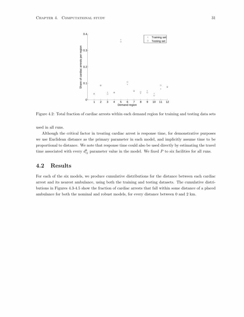
Chapter 4. Computational study 31
1 2 3 4 5 6 7 8 9 10 11 120
0.1
0.2
0.3
0.4
Demand region
Sha
re o
f car
diac
arr
ests
per
reg
ion
Training setTesting set
Figure 4.2: Total fraction of cardiac arrests within each demand region for training and testing data sets
used in all runs.
Although the critical factor in treating cardiac arrest is response time, for demonstrative purposes
we use Euclidean distance as the primary parameter in each model, and implicitly assume time to be
proportional to distance. We note that response time could also be used directly by estimating the travel
time associated with every dkij parameter value in the model. We fixed P to six facilities for all runs.
4.2 Results
For each of the six models, we produce cumulative distributions for the distance between each cardiac
arrest and its nearest ambulance, using both the training and testing datasets. The cumulative distri-
butions in Figures 4.3-4.5 show the fraction of cardiac arrests that fall within some distance of a placed
ambulance for both the nominal and robust models, for every distance between 0 and 2 km.

Chapter 4. Computational study 32
0 500 1000 1500 20000
0.2
0.4
0.6
0.8
1
Distance (m)
Fra
ctio
n o
f ca
rdia
c ar
rest
s
Nominal (p−median)
Robust (p−median)
(a) Training dataset
0 500 1000 1500 20000
0.2
0.4
0.6
0.8
1
Distance (m)
Fra
ctio
n o
f ca
rdia
c ar
rest
s
Nominal (p−median)
Robust (p−median)
(b) Testing dataset
Figure 4.3: Empirical cumulative distribution of distances between cardiac arrests and nearest ambulance- p-median models

Chapter 4. Computational study 33
0 500 1000 1500 20000
0.2
0.4
0.6
0.8
1
Distance (m)
Fra
cti
on
of
ca
rdia
c a
rrests
Nominal (CVaR)
Robust (CVaR)
(a) Training dataset
0 500 1000 1500 20000
0.2
0.4
0.6
0.8
1
Distance (m)
Fra
cti
on
of
ca
rdia
c a
rrests
Nominal (CVaR)
Robust (CVaR)
(b) Testing dataset
Figure 4.4: Empirical cumulative distribution of distances between cardiac arrests and nearest ambulance- CVaR models
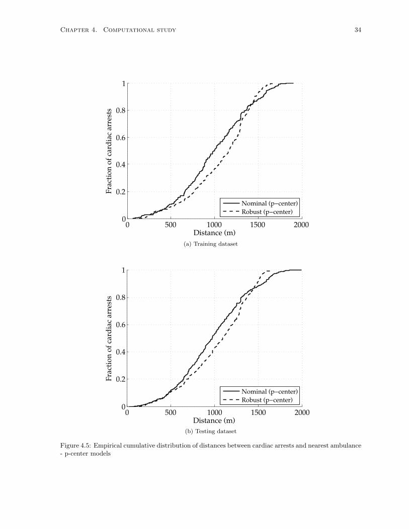
Chapter 4. Computational study 34
0 500 1000 1500 20000
0.2
0.4
0.6
0.8
1
Distance (m)
Fra
ctio
n o
f ca
rdia
c ar
rest
s
Nominal (p−center)
Robust (p−center)
(a) Training dataset
0 500 1000 1500 20000
0.2
0.4
0.6
0.8
1
Distance (m)
Fra
ctio
n o
f ca
rdia
c ar
rest
s
Nominal (p−center)
Robust (p−center)
(b) Testing dataset
Figure 4.5: Empirical cumulative distribution of distances between cardiac arrests and nearest ambulance- p-center models

Chapter 4. Computational study 35
We also use three distance metrics to evaluate the performance of each model: mean distance from
a cardiac arrest location to its nearest ambulance, the mean distance to the nearest ambulance of the
10% of “worst-served” cardiac arrests, and the maximum distance between any cardiac arrest and its
the nearest ambulance. These three metrics correspond to the objectives of the p-median, CVaR and
p-center location models, respectively. These results are shown for both the training set and the testing
set in Tables 4.1 and 4.2.
p-median CVaR (β = 90%) p-center
Distance metric (m) Nominal Robust Nominal Robust Nominal Robust
Mean 788.1 686.4 954.9 915.9 1003.4 1075.1CVaR (β = 90%) 1523.4 1422.7 1575.2 1387.3 1648.7 1541.2Max 2823.2 2469.9 2046.0 1676.0 1905.9 1676.0
Table 4.1: Performance of six location models on training dataset (506 cardiac arrests)
p-median CVaR (β = 90%) p-center
Distance metric (m) Nominal Robust Nominal Robust Nominal Robust
Mean 771.9 690.5 919.4 894.9 985.9 1039.4CVaR (β = 90%) 1471.1 1434.9 1572.2 1393.1 1665.9 1541.2Max 2688.1 2334.6 2046.0 1692.6 1998.2 1666.8
Table 4.2: Performance of six location models on test dataset (2023 cardiac arrests)
Table 4.3 shows a ranking of the six models based on each of the three distance metrics, where a
ranking of 1 is given to the model which achieves the best (lowest) distance metric. The rankings are
the same for both the testing and training data set.
Rank Mean 90%-CVaR Max
1 Robust p-median Robust CVaR Robust p-center2 Nominal p-median Robust p-median Robust CVaR3 Robust CVaR Nominal p-median Nominal p-center4 Nominal CVaR Robust p-center Nominal CVaR5 Nominal p-center Nominal CVaR Robust p-median6 Robust p-center Nominal p-center Nominal p-median
Table 4.3: Ranking of six models based on three distance metrics of test dataset

Chapter 4. Computational study 36
Lastly, in 4.6 we show the six optimal ambulance locations as determined by each of the three robust
location models.
!
!
!
!
!
!
!
!
!
!
!
!
!
!
!
!
!
!
!
!
!
!
!
!
!
!
!
!
!
!
!
!
!
!
!
!
!!
!
!
!
!
!
!
!
!
!
!
!
!
!
!
!
!
!
!
!
!
!
!
!
!
!
!
!
!
!
!
!
!
!
!
!
!
!
!
!
!
!
!
!
!
!
!
!
!
!
!
!
!
!
!
!
!
!
!
!
!
!
!
!
!
!
!
!
!
!
!
!
!
!
!
!
!
!
!
!
!
!
!
!
!
!
!
!!
!
!
!
!!
!
!
!
!
!
!
!
!
!
!
!
!
!
!
!
!
!
!
!
!
!
!
!
!
!!
!
!
!
!
!
!
!
!
!
!
!
!
!
!
!
!
!
!
!
!
!
!
!
!
!
!
!
!
!
!
!
!
!
! !
!
!
!
!
!
!
!
! !
!
!
!
!
!
!
!
!
!
!
!
!
!
!
!
!
!
!
!
!
!
!
!
!
!
!
!
!
!
!
!
!
!
!
!
!
!
!
!
!
!
!
!
!
!
!
!
!
!
!
!
!
!
!
!
!
!
!
!
!
!
!
!!
!
!
!
!
!
!
!
!
!
!
!
!
!
!
!
!
!
!
!
!
!
!
!
!
!
!
!
!
!
!
!
!
!
!
!
!
!!
!
!
!
!
!
!
!
!
!
!
!
!
!
!
!
!
!
!
!
!
!
!
!
!
!
!
!
!
!
!
!
!
!
!
!
!
!
!
!
!
!
!
!
!
!
!
!
!
!
!
!
!
!
!!
!
!
!
!
!
!
!
!
!
!
!
!
!
!
!
!
!
!
!
!
!
!
!
!
!
!
!
!
!
!
!
!
!
!
!
!
!
!
!
!
!
!
!
!
!
!
!
!!
!
!
!
!
!
!
!
!
!
!
!
!
!
!!
!
!
!
!
!
!
!
!
!
!
!
!
!
!
!
!
!
!
!
!
!
!
!
!
!
!
!
!
!
!
!
!
!
!
!
!
!
!
!
!
!
!
!
!
!
!
!
!
!
!
!!
!
!
!
!
!
!
!
!
!
!
!
!
!
!!
!
!
!
!
!
!
!
!
!
!
!
!
!
!
!
!
!
!
!!
!
!
!
!
!
!
!
!
!
!
!
!
!
!
!
!
!
!
!
!!
!
!
!
!
!
!
!
!
!
!
!
!
!
!
!
!
!
!
!
!
!
!
!
!
!
!
!
!
!
!
!
!
!!
!
!
!
!
!
!
! !
!
!
!
!
!
!
!
!
!
!
!
!
!
!
!
!
!
!
!
!
!
!
!
!
!
!
!
!
!
!
!
!
!
!
!
!
!
!
!
!
!
!!
!
!
!
!
!
!
!
!
!
!
!
!
!
!!
!
!
!
!
!
!
!
!
!
!
!
!
!
!
!
!
!
!
!
!
!
!
!
!
!
! !
!
!!
!
!
!
!
!
!
!
!
!
!
!
!
!
!
!
!
!
!
!
!
!
!
!
!
!
!
!
!
!
!
!
!
!
!!
!
!
!
!
!
!
!
!
!
!
!
!
!
!
!
!
!
!
!
!
!
!
!
!
!
!
! !
!
!
!
!
!
!
!
!
!
!
!
!
!
!
!
!
!
!
!
!
!
!
!
!
!
!
!
!
!
!
!
!
!
!
!
!
!
!
!
!
!
!
!
!
!
!
!
!
!!
!
!
!
!
!
!
!
!
!
!
!
!
!
!
!
!
!
!
!
!
!
!
!
!
!
!
!
!
!
!
!
!
!
!
!
!
!
!
!
!
!
!
!
!
!
!
!
!
!
!
!
!
!
!
!
!
!
!
!
!
!
!
!
!
!
!
!
!
!
!!
!
!
!
!
!
!
!
!
!
!
!
!
!
!
!
!
!
!
!
!
!
!
!
!
!
!
!
!
!
!
!
!
!
!
!
!
!
!
!
!
!
!
!
!
!!
!
!
!
!
!
!
!
!
!
!
!!
!
!
!
!!
!
!
!
!
!
!!
!
!
!
!
!
!
!
!
!
!
!!
!
!
!
!
!
!
!
!
!
!
!
!
!
!
! !
!
!
!
!
!
!
!
!
!
!
!
!
!
!
!
!
!
!
!
!
!
!
!
!
!
!
!
!
!
!
!
!
!
!
!
!
!
!
!
!
!
!
!
!
!
!
!
!
!
!
!!
!
!
!
!
!
!
!
!
!
!
!
!
!
!
!
!!
!
!
!
!!
!
!
!
!
!
!
!
!
!
!
!
!
!
!
!
!
!
!
!
!
!
!
!
!
!
!
!
!
!
!
!
!
!
!
!
!
!
!
!
!
!
!
!
!
!
!
!!
!
!
!
!
!
!
!
!
!
!
!
!
!!
!
!
!
!
!
!
!
!
!
!
!
!
!
!
!
!
!
!
!!
!
!
!
!
!
!!
!
!
!
!
!
!
!
!
!
!
!
!
!
!
!
! !
!
!
!
!!
!
!
!
!
!
!
!
!
!
!
!
!
!
!
!
!
!
!
!
!
!
!
!
!
!
!
!
!
!
!
!
!
!
!
!
!
!
!
!
!
!
!
!
!
!
!!
!
!
!
!
!
!
!
!
!
!
!
!
!
!
!!
!
!
!
!
!
!
!
!
!
!
!
!
!
!
!
!
!
!
!
!
!
!
!
!
!
!
!
!
!
!
!
!
!
!
!!
!
!
!
!
!
!
!
!
!
!
!
!
!
!
!
!
!
!
!
!
!
!
!
!
!
!
!
!
!
!
!
!
!
!
!
!
!
!
!
!
!
!
!
!
!
!
!
!
!
!
!
!
!
!
!
!
!
!
!
!
!
!
!
!
!
!
!
!
!
!
!
!
!
!
!
!
!
!
!
!
!
!
!
!
!
!
!
!
!
!
!
!
!
!
!
!
!
!
!
!
!
!
!
!
!
!
!
!
!
!
!
!
!!
!
!
!!
!
!
!
!
!
!
!
!
!
!
!
!
!
!
!
!
!
!
!
!
!
!
!
!
!
!!
!
!
! !
!
!
!
!
!
!
!
!
!
!
!
!
!
!
!
!
!
!
!
!
!
!
!
!
!
!
!
!
!
!
!
!
!
!
!
!
!
!
!
!
!
!
!
!
!
!!
!!
!
!
!
!
!
!
!
!
!
!
!
!!
!
!
!
!
!
!
!
!
!
!
!
!
!
!
!
!
!
!
!
!
!
!
!
!
!
!
!
!!
!
!
!
!
!
!
!
! !
!
!
!
!
!
!
!
!
!
!
!
!
!
!
!
!
!
!
!
!
!
!
!
!
!
!
!
!
!
!
!
!
!
!
!
!
!
!
!
!
!
!
!
!
!
!
!
!
!
!
!
!
!
!
!
!
!
!
!
!
!
!
!
!
!
!
!
!
!
!
!
!
!
!
!
!
!!
!
! !
!
!
!
!
!
!
!
!
!
!
!
!
!
!
!
!
!
!
!
!
!
! !
!
!
!
!
!
!
!
!
!
!
!
!
!
!
!
!
!
!
!
!
!
!
!
!
!
!
!
!
!
!
!
!
!
!
!
!
!
!
!
!
!
!
!
!
!
!
!
!
!
!
!
!
!
!
!
!
!
!
! !
!
!
!
!
!
!
!
!
!
!!
!
!
!
!
!
!
!
!
!
!
!
!
!
!
!
!
!
!
!
!
!
!
!
!
!
!
!
!
!
!
!
!
!
!
!!
!
!
!
!
!
!!
!
!
!
!
! !
!
!
!
!
!
!
!
!
!
!
!
!
!
!
!
!
!
!
!
!
!
!!
!
!
!
!
!
!
!
!
!
!
!
!
!
!
!
!!
!
!
!
!
!
!
!
!!
!
!
!
!
!
!
!
!
!
!
!
!
!
!
!
!
!
!
!
!
! ! !
!!
!
!
!
!
!
!
!
!
!
!
!
!
!
! !
!
!
!
!
!
!
!
!
!
!
!
!
!
!
!
!
!
!
!
!
!
!
!
!
!
!
!
!
!
!
!
!
!
!
!
!
!
!
!
!
!
!
!
!
!
!!
!
!
!
!
!
!
!
!
!
!
!
!
!
!
!
!
!
!
!
!
!
!
!
!
!
!
!
!
!
!
!
!
!
!
!
!
!
!
!
!
!
!
!
!
!
!
!
!
!
!
!
!
!
!
!
!
!
!
!
!
!
!
!
!
!
!
!
!
!
!
!
!
!
!
!
!
!
!
!
!
!
!
!
!
!
!
!
!
!
!
!
!
!
!
!
!
!
!
!
!
!
!
!
!
!
!
!
!
!
!
!
!
!
!
!
!
!
!
!
!
!
!
!
!
!
!
!
!
!
!
!
!
!
!
!
!
!
!
!
!
! !
!
!
!
!
!
!
!
!
!
!
!
!
!
!
!
!
!
!
!
!
!
!
!
!
!
!
!
!
!
!
!
!
!
!
!
!
!
!
!
!
!
!
!
!
!
!
!
!
!
!
!
!
!
!
!
!
!
!
!
!
!
!
!
!
!
!
!
!
!
!
!
!
!
!
!
!
!
!
!
!
!
!
!
!
!
!
!
!
!
!
!
!
!
!
!
!
!
!
!
!
!
!
!
!
!!
!
!
!
!
!
!
!
!
!
!
!
!
!
!
!
!
!
!
!
!
!
!
!
!
!
!
!
!
!
!
!
!
!
!
!
!
!!
!
!
!!
!
!
!
!
!
!
!
!
!
!
!
!
!
!
!
!
!
!
!
!
!
!
!
!
!
!
!
!
!
!
!
!
!
!
!
!
!
!
! !
!
!
!
!
!
!
!
!
!
!
!
!
!
!
!
!!
!
!
!! !
!
!
!
!
!
!
!
!
!
!
!
!
!
!
!
!!
!
!
!
!
!
!
!
!
!
!
!
!
!
!
!
!
!
!
!
!
!
!
!
!
!
!
!
!
!
!
!
!
!
!
!
!
!
!
!
!
!
!
!
!
!
!
!
!
!
!
!
!
!
!
!
!
!!
!
!
!
!
!
!
!
!
!
!
!
!
!
!
!
!
!
!
!
!
!!
!!
!
!
!
!
!
!
!
!
!
!
!
!
!
!
!
!
!
!
!
!
!
!!
!!
!
!!
!
!
!
!
!
!
!!
!
!
!
!!
!
!
!
!
!
!
!
!
!
!
!
!
!
!
!
!
!
!
!
!
!
!
!
!
!
!
!
!
!
!
!
!
!
!
!
!
!
!
!
!
!
!
!
!
!
! !
!
!
!
!
!
!
!
!
!
!
!
!
!
!
!
!
!
!
!
!
!
!
!
!
!
!
!
!
!
!
!
!
!
!
!
!
!
!
!
! !
!!
!
!
!
!
!
!
!!
!
!
!
!
!
!
!
!
!
!
!
!
!
!
!
!
!
!
!
!
!
!
!
!
!
!
!
!
!
!
!
!
!
!!
!
!
!
!
!
!
!
!
!
!
!
!
!
!
!
!
!
!
!
!
!
!
!
!
!
!
!
!
!
!
!
!
!
!!
!
!
!
!
!
!
!
!
!
!
!
!
!
!
!
!
!
!
!
!!
!
!
!!
!
!
!
!
!
!
!
!
!
[
[
[[
[
[
E
E
E
E
E
E
*
*
*
*
*
*
1 Km
Legend* Robust p-medianE Robust CVaR
[ Robust p-center! Cardiac arrest locations
Figure 4.6: Locations of six facilities placed by robust p-median, robust CVaR and robust p-centerlocation models
4.3 Discussion
Although we used straight-line distances as a proxy for ambulance accessibility in our study, previous
work in the medical literature suggests a high correlation between straight-line distance and travel time
(Phibbs and Luft, 1996; Haynes et al., 2006). This is particularly true for ambulances which, in North
America, are generally unimpeded by traffic congestion. We therefore posit that the improvements
in straight-line distance shown in our results are likely to correspond with real improvements in EMS
response time. However, it may still be beneficial to compare these results with an identical study which
uses road distance or estimated travel time.
Figure 4.3 shows that the distribution of the robust p-median tends to dominate the nominal p-
median model at all distances. Similarly, the robust model performs better (produces lower distance
values) than the nominal model when measured by average distance, the CVaR distance or maximum
distance. Figure 4.4 shows that the robust CVaR does nto necessarily perform better than the nominal
model, except for cardiac arrests above the 65th percentile of the distribution, beyond which the robust
model visibly dominates. However, the robust CVaR model still outperforms the nomimal CVaR model
on all three distance metrics. Lastly, the robust p-center model outperforms the nominal model beyond
the 85th percentile, but significantly underperforms at lower distances. This is an intuitive result given
that our implementation of the robust p-center model focuses improving service for the single point in

Chapter 4. Computational study 37
the entire study region that is furthest from any facility. This also results in the robust p-center model
producing a higher mean distance that the nominal formulation.
Unsurprisingly, the model that achieves the best performance when measured by the mean, CVaR
and maximum distance metrics are the robust p-median, robust CVaR and robust p-center models,
respectively. Despite performing the best when measured by mean distance, the two p-median models
rank last when measured by the maximum distance metric. This is an expected outcome, given that the
goal of the p-median models is to minimize expected distance, whereas the CVaR and p-center models
focus on improving performance at the tail of the distribution.
The rankings of the six models shown in 4.3 reiterate that the robust models all outperform their
corresponding nominal models on each of their respective distance metrics. Further, comparing robust
and nominal formulations for all three models across each of the three distance metrics provides a total
of nine possible “robust vs nominal” comparisons. In eight of these, the robust model achieves a higher
ranking than its nominal counterpart. Only the nominal p-center performs better than the robust
formulation on the mean distance metric, suggesting the robust p-center might be overly conservative.
From the rankings, we also observe that the robust CVaR model is in the top 3 for each of the distance
metrics. This suggests that minimizing the tail-average serves as a good compromise between minimizing
the average of the entire distribution and minimizing the maximum value. As a consequence, if there
is uncertainty regarding which of the the three metric is most important is when optimizing the facility
locations, the robust CVaR might be an appropriate choice as a result of its strong performance in all
cases.
With respect to the facility locations themselves, Figure 4.6 shows that the facility that is furthest
North, South, East or West within the study region are all placed by the robust p-center model (although
the p-median model also places a facility at the same site as the northern most p-center facility). This
reflects the fact that the p-center model focuses on minimizing distance for the absolute “worst-served”
point on the map, which causes the optimal locations to be relatively more spread out. By contrast,
the robust p-median model places two facilities in the region with the highest number of cardiac arrests,
whereas the other two models place no facilities in this region.
While the exact risk of cardiac arrest throughout the study region is unknown, the empirical distribu-
tions can provide an estimate of the probability that a random cardiac arrest will occur within x metres
of one of the ambulance locations. The similarities between the training and testing distributions suggest
that, in aggregate, historical data can provide a reasonably accurate estimate of the future distribution
of cardiac arrest locations.

Chapter 5
Conclusion
In this thesis, we presented a two-stage robust optimization framework for modeling demand location
uncertainty in multi-facility location problems. We have shown our methods to be generalizable by
applying it to the classical p-median and p-center problems – two of the most studied models in the
facility location literature. We also presented a novel location model based on conditional value-at-risk
(CVaR), which we also modify to account for demand location uncertainty. We also discussed how the
p-median and p-center models can be viewed as special cases of the CVaR model, which shows that the
robust CVaR model itself represents a family of models that works within our uncertainty framework.
This grants a decision maker the flexibility to tailor the optimization to different parts of the distance
distribution by selecting appropriate parameter values in the CVaR formulation. While we only consider
ambulance positioning in this thesis, modeling demand location uncertainty is likely to be beneficial in
other real world problems, such as the location of fire stations, public access defibrillators or treatment
centers for medical evacuation.
To solve our robust optimization models, we proposed a decomposition algorithm based on row-and-
column generation. Notably, the efficiency of algorithm allows us to closely approximate continuous
uncertainty regions by using a scenario-based approach to modeling the uncertainty. Further, our dis-
cretization approach is general and allows uncertainty regions to take on any shape.
In our final chapter, we performed a computational study on strategic ambulance positioning. Our
study was motivated by the uncertainty in the location of future emergencies when ambulance positioning
decisions are made. Additionally, our data shows that it may be more accurate to model ambulance
demand as continuous in space rather than concentrated at a finite number of demand nodes. Our
results suggest that our approach may lead to improvements in response time, particularly for those
emergencies which occur the furthest from any ambulance location. Given the well established link
between ambulance response time and the chances of survival from cardiac arrest, hedging against
uncertainty in this instance may have a positive and tangible impact on health and human life.
With respect to future work, it may be beneficial to incorporate some measure of control over the
conservatism of our robust optimization formulations. The models developed in this thesis assume that
demands will always be realized in the locations that are furthest from existing facilities. While this
allows us to hedge against worst-case realizations of demand, it may cause the system to perform poorly
for typical cases. Allowing for some control over the conservatism of the uncertainty regions may further
improve our robust optimization models. This may be done by enforcing additional constraints which
38
Chapter 5. Conclusion 39
limit the demand distribution from taking on overly conservative forms.
Additionally, it may be valuable to examine whether our uncertainty framework can be incorporated
into other location models. Although we focused primarily on classical formulations, it is conceivable
that our approach might also extend to location models which consider facility reliability or capacity.
This would further broaden the scope of this work.
Lastly, given the focus on modeling demand, our computational study takes a fairly straightforward
approach to modeling ambulance behaviour. The existing ambulance literature takes a more nuanced
approach to modeling the ambulances, by incorporating uncertain travel times, ambulance busy proba-
bilities, multiple vehicle types and dynamic relocation into the models. However, it is our hope that this
study serves as a reminder of why the demands themselves should also be modelled in a realistic man-
ner. To the best of our knowledge, our incorporation of uncertainty in demand locations is novel within
the general facility location literature, and therefore is also novel among existing ambulance location
models. A logical next step would be to combine advanced modeling of ambulance behaviour with our
model for demand location uncertainty. In our view, improving the response to cardiac arrest through
ambulance location optimization requires that we continue to account for uncertainty in the real world.
This includes uncertainty in the behaviour of the facilities as well as the demands themselves.

Bibliography
Alper Atamturk and Muhong Zhang. Two-stage robust network flow and design under demand uncer-
tainty. Operations Research, 55(4):662–673, 2007.
Igor Averbakh and Sergei Bereg. Facility location problems with uncertainty on the plane. Discrete
Optimization, 2(1):3–34, 2005.
Michael O. Ball and Feng L. Lin. A reliability model applied to emergency service vehicle location.
Operations Research, 41(1):18–36, 1993.
Nathaniel Bastian. A robust, multi-criteria modeling approach for optimizing aeromedical evacuation
asset emplacement. The Journal of Defense Modeling and Simulation: Applications, Methodology,
Technology, 7(1):5–23, 2010.
Aharon Ben-Tal, Alexander Goryshko, E. Guslitzer, and Arkadi Nemirovski. Adjustable robust solutions
of uncertain linear programs. Mathematical Programming, 99(2):351–376, 2004.
Oded Berman, Iman Hajizadeh, and Dmitry Krass. The maximum covering problem with travel time
uncertainty. IIE Transactions, 45(1):81–96, 2013.
Dimitris Bertsimas, David Brown, and Constantine Caramanis. Theory and applications of robust
optimization. SIAM Review, 53(3):464–501, 2011.
Luce Brotcorne, Gilbert Laporte, and Frederic Semet. Ambulance location and relocation models.
European journal of operational research, 147(3):451–463, 2003.
Gerald Brown, Matthew Carlyl, Javier Salmeron, and Kevin Wood. Defending critical infrastructure.
Interfaces, 36(6):530–544, 2006.
Gerald G. Brown, W. Matthew Carlyle, Robert C. Harney, Eric M. Skroch, and R. Kevin Wood. Inter-
dicting a nuclear-weapons project. Operations Research, 57(4):866–877, 2009.
Timothy C.Y. Chan, Heyse Li, Gerald Lebovic, Sabrina K. Tang, Joyce Y.T. Chan, Horace C.K. Cheng,
Laurie J. Morrison, and Steven C. Brooks. Identifying locations for public access defibrillators using
mathematical optimization. Circulation, 127(17):1801–1809, 2013.
Gang Chen, Mark S. Daskin, Zuo-Jun Max Shen, and Stanislav Uryasev. The -reliable mean-excess
regret model for stochastic facility location modeling. Naval Research Logistics, 53, 2006.
Richard Church and Charles ReVelle. The maximal covering location problem. Papers in regional
science, 32(1):101–118, 1974.
40

BIBLIOGRAPHY 41
Leon Cooper. Bounds on the weber problem solution under conditions of uncertainty. Journal of Regional
Science, 18(1):87–92, 1978.
Tingting Cui, Yanfeng Ouyang, and Zuo-Jun Max Shen. Reliable facility location design under the risk
of disruptions. Operations Research, 58(4):998–1011, 2010.
Mark S Daskin. A maximum expected covering location model: formulation, properties and heuristic
solution. Transportation Science, 17(1):48–70, 1983.
Mark S. Daskin and Edmund H. Stern. A hierarchical objective set covering model for emergency medical
service vehicle deployment. Transportation Science, 15(2):137–152, 1981.
Zvi Drezner. Stochastic analysis of the weber problem on the sphere. Journal of the Operational Research
Society, pages 1137–1144, 1989.
Erhan Erkut, Armann Ingolfsson, and Gne Erdoan. Ambulance location for maximum survival. Naval
Research Logistics, 55(1):42–58, 2008.
Michel Gendreau, Gilbert Laporte, and Frdric Semet. Solving an ambulance location model by tabu
search. Location Science, 5(2):75–88, 1997a.
Michel Gendreau, Gilbert Laporte, and Frdric Semet. A dynamic model and parallel tabu search heuristic
for real-time ambulance relocation. Parallel computing, 27(12):1641–1653, 1997b.
Jeffrey Goldberg, Robert Dietrich, Jen Ming Chen, M. George Mitwasi, Terry Valenzuela, and Elizabeth
Criss. Validating and applying a model for locating emergency medical vehicles in tuczon, az. European
Journal of Operational Research, 49(3):308–324, 1990.
Robin Haynes, Andrew P. Jones, Violet Sauerzapf, and Hongxin Zhao. Validation of travel times to
hospital estimated by gis. International Journal of Health Geographics, 5(1):40, 2006.
M Larsen, M Eisenberg, RO Cummins, and AP Hallstrom. Predicting survival from out-of-hospital 309
cardiac arrest: a graphic model. Annals of Emergency Medicine, (22):1652–1658, 1993.
Eva K. Lee, Siddhartha Maheshwary, Jacquelyn Mason, and William Glisson. Large-scale dispensing for
emergency response to bioterrorism and infectious-disease outbreak. Interfaces, 36(6):591–607, 2006.
Michael Lim, Mark Dasin, Achal Bassamboo, and Sunil Chopra. A facility reliability problem: Formu-
lation, properties, and algorithm. Naval Research Logistics, 57(1):58–70, 2010.
Marvin B Mandell. Covering models for two-tiered emergency medical services systems. Location Science,
6(1):355–368, 1998.
Vladimir Marianov and Charles ReVelle. The queueing maximal availability location problem: a model
for the siting of emergency vehicles. European Journal of Operational Research, 93(1):110–120, 1993.
G Nichol, E Thomas, and CW Callaway. Regional variation in out-of-hospital cardiac arrest incidence
285 and outcome. JAMA, (300):1423–1431, 2008.
Susan Hesse Owen and Mark S. Daskin. Strategic facility location: A review. European Journal of
Operational Research, 111(3), 1998.

BIBLIOGRAPHY 42
Praveen Paruchuri, Jonathan P. Pearce, Janusz Marecki, Milind Tambe, Fernando Ordonez, and Sarit
Kraus. Playing games for security: an efficient exact algorithm for solving bayesian stackelberg games.
Proceedings of the 7th international joint conference on Autonomous agents and multiagent systems,
2:895–902, 2008.
Jill P. Pell, Jane M. Sirel, Andrew K. Marsden, Ian Ford, and Stuart M. Cobbe. Effect of reducing
ambulance response times on deaths from out of hospital cardiac arrest: cohort study. BMJ, 322
(7299):1385–1388, 2001.
Ciaran S. Phibbs and Harold S. Luft. Correlation of travel time on roads versus straight line distance.
Medical Care Research and Review, 52(4):532–542, 1996.
John F. Repede and John J. Bernardo. Developing and validating a decision support system for locating
emergency medical vehicles in louisville, kentucky. European Journal of Operational Research, 75(3):
567–581, 1994.
Charles ReVelle and Kathleen Hogan. The maximum availability location problem. Transportation
Science, 23(3):192–200, 1989.
R. Tyrrell Rockafellar and Stanislav Uryasev. Optimization of conditional value-at-risk. Journal of Risk,
2000.
Comilla Sasson, Carla C. Keirns, Dylan Smith, Michael Sayre, Michelle Macy, William Meurer, Bryan F.
McNally, Arthur L. Kellermann, and Theodore J. Iwashyna. Small area variations in out-of-hospital
cardiac arrest: does the neighborhood matter? Annals of internal medicine, 153(1):19–22, 2010.
David Schilling, D. Jack Elzinga, Jared Cohon, Richard Church, and Charles ReVelle. The team/fleet
models for simultaneous facility and equipment siting. Transportation Science, 13(2):163–175, 1979.
Zuo-Jun Max Shen, Roger Lezhou Zhan, and Jiawei Zhang. The reliable facility location problem:
Formulations, heuristics, and approximation algorithms. INFORMS Journal on Computing, 23(3):
470–482, 2011.
Auyon A. Siddiq, Steven C. Brooks, and Timothy C.Y. Chan. Modeling the impact of public access
defibrillator range on public location cardiac arrest coverage. Resuscitation, 2012.
Lawrence V. Snyder. Facility location under uncertainty: A review. IIE Transactions, 38(7):547–564,
2006.
Barbaros C. Tansel, Richard L. Francis, and Timothy J. Lowe. State of the artlocation on networks: A
survey. part i: The p-center and p-median problems. Management Science, 29(4):482–497, 1983.
Constantine Toregas, Ralph Swain, Charles ReVelle, and Lawrence Bergman. The location of emergency
service facilities. Operations Research, 19(6):1363–1373, 1971.
Godfried T. Toussaint. Computing largest empty circles with location constraints. International Journal
of Parallel Programming, 12(5):347–358, 1983.
TD Valenzuela, DJ Roe, G Nichol, LL Clark, DW Spaite, and RG Hardman. Outcomes of rapid 298
defibrillation by security officers after cardiac arrest in casinos. New England Journal of Medicine,
(343):1206–1209, 2000.

BIBLIOGRAPHY 43
ML Weisfeldt, CM Sitlani, JP Ornato, T Rea, TP Aufderheide, D Davis, J Dreyer, EP Hess, J Jui, J Mal-
oney, G Sopko, J Powell, G Nichole, and LJ Morrison. Survival after 289 application of automatic
external defibrillators before arrival of the emergency medical system: 290 evaluation in the resusci-
tation outcomes consortium population of 21 million. Journal of the American College of Cardiology,
(55):1713–1720, 2010.

Appendix A
Proofs
Lemma 1 The optimal values of (2.2) and (2.3) are equal.
Proof: The feasible sets Y and X are the same in both formulations, so we only require that for a
feasible (y, x)
minz∈Z2
∑i∈I
∑k∈Kj
∑j∈J
hjdkijz
kij = min
z∈Z3
∑i∈I
∑k∈Kj
∑j∈J
hjdkijz
kij x
kj
where Z2 and Z3 are the feasible regions for z in (2.2) and (2.3) given y, respectively. Since Z2 is
separable in j, we have
minz∈Z2
∑i∈I
∑k∈Kj
∑j∈J
hjdkijz
kij =
∑j∈J
minz∈Z2j
∑i∈I
∑k∈Kj
hjdkijz
kij
The same holds for Z3. Now we show that for any j,
minz∈Z2j
∑i∈I
∑k∈Kj
hjdkijz
kij = min
z∈Z3j
∑i∈I
∑k∈Kj
hjdkijz
kij x
kj
Let I ={i | yi = 1
}and Kj =
{k | xkj = 1
}. First, we consider (2.2). Since
∑i∈I
∑k∈Kj
zkij = 1, ∀j ∈ J and
zj ∈ {0,1}, we have
minz∈Z2
∑i∈I
∑k∈Kj
hjdkijz
kij = min
i∈I, k∈Kj
{hjd
kij
}
Similarly, for (2.3), since∑i∈I z
kij = 1, and
∑k∈Kj
xkj = 1, and xj ∈ {0,1}, we obtain
minz∈Z3
∑i∈I
∑k∈Kj
hjdkijz
kij x
kj = min
i∈I
{ ∑k∈Kj
hjdkij x
kj
}= mini∈I,k∈Kj
{hjd
kij
}. �
Lemma 2 For a feasible y, the inner max-min problem in (2.3) contains a saddle point.
Proof: We are required to show that f(x, z∗) ≤ f(x∗, z∗) ≤ f(x∗, z). Since f(x, z) is concave (linear)
in x, we have f(x, z∗) ≤ maxx∈X f(x, z∗) = f(x∗, z∗), which proves the first inequality. Similarly,
since f(x, z) is convex (linear) in z, we have minz∈Z f(x∗, z) = f(x∗, z∗) ≤ f(x∗, z), proving the second
inequality. �
44

Appendix A. Proofs 45
Lemma 3 For a fixed y, the optimal value of (2.3) remains unchanged when the integrality constraints
on x and z are relaxed.
Proof: We are required to show that there exists an optimal solution in the relaxed formulation where
x∗ and z∗ are binary. Due to separability, we can consider an arbitrary demand j in both cases. For x,
we note that relaxation of the binary constraint yields Xj = {xkj |∑k x
kj = 1,x ≥ 0} where X =
∏j Xj .
Since, for an arbitrary j, Xj defines the |K| − 1 dimensional simplex, all corner points of Xj are binary,
and so any optimal x∗ must be binary.
Now we consider the relaxation on z. With the binary constraint relaxed and replaced with non-
negativity constraints, Zj is given by {zkij |∑i zkij = 1,∀k ∈ Kj , z
kij ≤ yi,∀i, j, k}. For there to exist an
optimal z that is non-integer, one of the binding constraint on z must have a non-integer right hand
side. However, all constraints on z have a RHS value of 0 or 1, meaning z must be binary at every corner
point of Z.
Lemma 4 The optimal values of (2.12) and (2.13) are equal.
Proof: Let g(α,x, z) = α + 11−β
∑j∈J hj max {fj(xj , zj)− α, 0}. Let xj = argmax
xj
fj(xj , zj), and
x =∏j∈J xj . The feasible sets for Y and Z(y) are the same in both formulations, so we are required to
show that for a feasible z,
maxx
minαg(α,x, z) = min
αg(α,x, z)
Since the feasible set for x is the same in (2.12) and (2.13), we obtain the following inequality
maxx
minαg(α,x, z) ≥ min
αg(α,x, z)
Now we consider the reverse direction. Since for any solution (α, x), we obtain f(xj , zj) ≤ f(xj , zj),
this implies
max {fj(xj , zj)− α, 0} ≤ max {fj(xj , zj)− α, 0}
Which gives us g(α, x, z) ≤ g(α,x, z) for any (α, x). Now, let (α1,x1) and (α2,x2) be the optimal
solutions to (2.12) and (2.13), respectively. Since x2 = x, we finally obtain
maxx
minαg(α,x, z) = g(α1,x1, z) ≤ g(α2,x1, z) ≤ g(α2,x, z) = min
αg(α,x, z). �