Robust Euclidean Embedding via EDM Optimization · all other three problems, when reformulated in...
43
Noname manuscript No. (will be inserted by the editor) Robust Euclidean Embedding via EDM Optimization Shenglong Zhou · Naihua Xiu · Hou-Duo Qi Received: March 20, 2018/ Accepted: date Abstract This paper aims to propose an efficient numerical method for the most challenging problem known as the robust Euclidean embedding (REE) in the fam- ily of multi-dimensional scaling (MDS). The problem is notoriously known to be nonsmooth, nonconvex and its objective is non-Lipschitzian. We first explain that the semidefinite programming (SDP) relaxations and Euclidean distance matrix (EDM) approach, popular for other types of problems in the MDS family, failed to provide a viable method for this problem. We then propose a penalized REE (PREE), which can be economically majorized. We show that the majorized prob- lem is convex provided that the penalty parameter is above certain threshold. Moreover, it has a closed-form solution, resulting in an efficient algorithm dubbed as PREEEDM (for Penalized REE via EDM optimization). We will prove among oth- ers that PREEEDM converges to a stationary point of PREE. Finally, the efficiency of PREEEDM will be compared with several state-of-the-art methods including SDP and EDM solvers on a large number of test problems from sensor network localization and molecular conformation. Keywords Euclidean embedding · Euclidean distance matrix · matrix optimiza- tion · majorization and minimization method Mathematics Subject Classification (2000) 49M20 · 65B05 · 90C26 · 90C30 · 90C52 Shenglong Zhou School of Mathematics, University of Southampton. Southampton SO17 1BJ, UK. E-mail: [email protected] Naihua Xiu Department of Applied Mathematics, Beijing Jiaotong University, Beijing, China. E-mail: [email protected] Hou-Duo Qi School of Mathematics, University of Southampton, Southampton SO17 1BJ, UK. E-mail: [email protected]
Transcript of Robust Euclidean Embedding via EDM Optimization · all other three problems, when reformulated in...

Noname manuscript No.(will be inserted by the editor)
Robust Euclidean Embedding via EDM Optimization
Shenglong Zhou · Naihua Xiu · Hou-Duo Qi
Received: March 20, 2018/ Accepted: date
Abstract This paper aims to propose an efficient numerical method for the mostchallenging problem known as the robust Euclidean embedding (REE) in the fam-ily of multi-dimensional scaling (MDS). The problem is notoriously known to benonsmooth, nonconvex and its objective is non-Lipschitzian. We first explain thatthe semidefinite programming (SDP) relaxations and Euclidean distance matrix(EDM) approach, popular for other types of problems in the MDS family, failedto provide a viable method for this problem. We then propose a penalized REE(PREE), which can be economically majorized. We show that the majorized prob-lem is convex provided that the penalty parameter is above certain threshold.Moreover, it has a closed-form solution, resulting in an efficient algorithm dubbedas PREEEDM (for Penalized REE via EDM optimization). We will prove among oth-ers that PREEEDM converges to a stationary point of PREE. Finally, the efficiency ofPREEEDM will be compared with several state-of-the-art methods including SDP andEDM solvers on a large number of test problems from sensor network localizationand molecular conformation.
Keywords Euclidean embedding · Euclidean distance matrix · matrix optimiza-tion · majorization and minimization method
Mathematics Subject Classification (2000) 49M20 · 65B05 · 90C26 ·90C30 · 90C52
Shenglong ZhouSchool of Mathematics, University of Southampton. Southampton SO17 1BJ, UK.E-mail: [email protected]
Naihua XiuDepartment of Applied Mathematics, Beijing Jiaotong University, Beijing, China.E-mail: [email protected]
Hou-Duo QiSchool of Mathematics, University of Southampton, Southampton SO17 1BJ, UK.E-mail: [email protected]

2 Zhou, Xiu and Qi
1 Introduction
This paper aims to propose an efficient numerical method for the most challengingproblem in the Multi-Dimensional Scaling (MDS) family, which has found manyapplications in social and engineering sciences [6, 10]. The problem is known asthe Robust Euclidean Embedding, a term borrowed from [8]. In the following, wefirst describe the problem and its three variants. We then explain our approachand our main contribution. We will postpone the relevant literature review to thenext section in order to shorten the introduction part.
1.1 Problem description
The problem can be described as follows. Suppose we are given some dissimilaritymeasurements (e.g., noisy distances), collectively denoted as δij , for some pairs(i, j) among n items. The problem is to find a set of n points xi ∈ <r, i = 1, . . . , nsuch that
dij := ‖xi − xj‖ ≈ δij (i, j) ∈ E , (1)
where ‖x‖ is the Euclidean norm (i.e., `2 norm) in <r and E is the set of the pairs(i, j), whose dissimilarities δij > 0 are known (E can be thought of the edge set ifwe treat δij as a weighted edge distance between vertex i and vertex j, resultingin a weighted graph.) Throughout, we use “:=” or “=:” to mean “define”. Thespace <r is called an embedding space and it is most interesting when r is small(e.g., r = 2, 3 for data visualization). One may also try to find a set of embeddingpoints such that the squared distances approximate the squared δ2
ij :
Dij := ‖xi − xj‖2 ≈ δ2ij (i, j) ∈ E . (2)
A great deal of effort has been made to seek the best approximation from (1) or(2). The most robust criterion to quantify the best approximation is the RobustEuclidean Embedding (REE) defined by
minX
f (d,1)(x1, . . . ,xn) :=n∑
i,j=1
Wij |dij − δij |, (3)
where Wij > 0 if δij > 0 and Wij ≥ 0 otherwise (Wij can be treated as a weightfor the importance of δij), and X := [x1, . . . ,xn] with each xi being a columnvector. In [1, 8], Problem (3) was referred to as a robust variant of MDS and isdenoted as rMDS. We will reserve rMDS for the Robust MDS problem:
minX
f (D,1)(x1, . . . ,xn) :=n∑
i,j=1
Wij |Dij − δ2ij |. (4)
The reference rMDS for the problem (4) is more appropriate because it involvedthe squared distances Dij , which were used by the classical MDS [22, 42, 48, 52].The preceding two problems are robust because of the robustness of the `1 normused to quantify the errors [30, Sect. IV].
Robust Euclidean Embedding 3
When the least squares criterion is used to (1), we have the popular modelknown as the Kruskal’s stress [29] minimization:
minX
f (d,2)(x1, . . . ,xn) :=n∑
i,j=1
Wij
(dij − δij
)2, (5)
Similarly, when the least-squares criterion was applied to (2), we get the so-calledsquared stress [6]:
minX
f (D,2)(x1, . . . ,xn) :=n∑
i,j=1
Wij
(Dij − δ2
ij
)2, (6)
In many applications such as molecular conformation [21], lower and upperbounds data on the distances can also be collected:
Lij ≤ Dij ≤ Uij , ∀ (i, j), (7)
where 0 ≤ Lij ≤ Uij . In applications such as nonlinear dimensionality reduction[46] and sensor network localization [43, 53], upper bounds Uij can be computedby the shortest path distances and Lij are simply set to be zero.
According to [8, Sect. 5.1], all of those problems are NP-hard. However, someproblems are computationally more “difficult” to solve than the others. The mostchallenging one, which is also the main focus of this paper, is the problem (3)with/without the constraint (7). The difficulty comes from the nonsmooth termof `1 norm and the distance terms dij used. All other problems either involvethe squared distances Dij or the squared `2 norm, which make them “easier” toapproximate. We will explain the reasons in the literature review part.
In contrast to all other three problems, there lacks efficient methods for theREE problem (3). One of the earliest computational papers that discuss this prob-lem is Heiser [23], which is followed up by [28], where the Huber smoothing functionwas used to approximate the `1 norm near zero with a majorization technique. Itwas emphasized in [28] that “the function is not differentiable at its minimum andis hard to majorize, leading to a degeneracy that makes the problem numericallyunstable”. Another important method is the PlaceCenter (PC for short) algorithmstudied in [1]. We will compare with it in the numerical part. The difficulty insolving (3) is also well illustrated by a sophisticated Semi-definite Programming(SDP) approach in [34, Sect. IV] (see the literature review part). We now describeour approach proposed in this paper.
1.2 Our approach and main contributions
Our approach heavily makes use of the concept of Euclidean Distance Matrix(EDM). We need some notation. Let Sn denote the space of all n× n symmetricmatrices, endowed with the standard inner product. The induced norm is theFrobenius norm, denoted by ‖A‖ for A ∈ Sn. The (i, j)th element of A ∈ Sn isoften written as Aij . Let Sn+ be the cone of positive semidefinite matrices in Snand we write A � 0 for A ∈ Sn+. A matrix D ∈ Sn is called an EDM if thereexists a set of points xi ∈ <r, i = 1, 2 . . . , n such that the (i, j)th element of D isgiven by Dij := ‖xi − xj‖2, i, j = 1, . . . , n. The smallest dimension r is called the

4 Zhou, Xiu and Qi
embedding dimension of D and r = rank(JDJ), where J := I− 1n11T is known as
the centring matrix with I being the identity matrix in Sn and 1 being the vectorof all ones in <n. We use Dn to denote the set of all Euclidean distance matricesof size n× n.
A very useful characterization for D ∈ Dn [22, 48] is
diag(D) = 0 and − (JDJ) � 0. (8)
This result shows that Dn is a closed and convex cone. Moreover, a set of embed-ding points are generated by the classical MDS method [22,42,48,52]:
[x1,x2, . . . ,xn] = diag(√λ1,√λ2, . . . ,
√λr) [p1,p2, . . . ,pr]
T , (9)
where the eigenvalues λ1 ≥ λ2 ≥ · · · ≥ λr > 0 and the corresponding eigenvectorsp1,p2, . . . ,pr are from the eigen-decomoposition:
− 1
2(JDJ) = [p1,p2, . . . ,pr] diag(λ1, λ2, . . . , λr) [p1,p2, . . . ,pr]
T (10)
with r = rank(JDJ). Therefore, the REE problem (3) with the constraint (7) canbe reformulated in terms of EDM as
minD f(D) :=∑ni,j=1Wij |
√Dij − δij | = ‖W ◦ (
√D −∆)‖1
s.t. D ∈ Dn, rank(JDJ) ≤ rD ∈ B := {A | L ≤ D ≤ U} ,
(11)
where “◦” is the Hadamard product for matrices (i.e., A ◦ B = (AijBij)),√D is
the elementwise square root of D, ∆ij := δij , and ‖ · ‖1 is the `1 norm. Once weobtained an optimal solution of (11), we use (9) and (10) to generate the requiredembedding points.
The reformulation well captures the four difficulties in solving the REE problem(3).
(i) The objective function f(D) is not convex. The term |√Dij − δij | is convex
when δ2ij > Dij and concave otherwise.
(ii) The objective function is nonsmooth. It is not differentiable at certain pointsdue to the `1 norm and the square root operation involved.
(iii) The objective function is not Lipschizian. The Lipschitz constant goes to in-finity as Dij goes to zero. The implication is that the subdifferential of theobjective function [41, Def. 8.3] may be unbounded. This would create a hugeobstacle in establishing any convergence results of iterative algorithms for (11).
(iv) The rank constraint is not convex and is hard to approximate. This is a commonissue for any optimization problem with a rank constraint.
We note that no matter what reformulations one may use for (3), those fourdifficulties would appear in different forms and won’t go away. We also note thatall other three problems, when reformulated in terms of EDM, have a convexobjective function. This distinctive feature alone makes the problem (11) the mostchallenging one to solve.
Existing numerical experiments have evidenced that the MDS embedding (9)and (10) works well as long as D is close to a true EDM. A typical example iswhen the data sits on a lower-dimensional manifold [46]. Motivated by this, we are
Robust Euclidean Embedding 5
going to generate an approximate EDM instead of a true EDM in our algorithm.It follows from (8) that (also see [31, Thm. A]):
D ∈ Dn ⇐⇒ diag(D) = 0 and −D ∈ Kn+, (12)
where Kn+ is known to be the conditionally positive semidefinite cone:
Kn+ :={A ∈ Sn | vTAv ≥ 0, ∀ v ∈ 1⊥
}and 1⊥ is the subspace in <n orthogonal to 1. The diagonal constraint in (12)can be integrated to the set B with the choice Lii = Uii = 0 for i = 1, . . . , n. Wecombine Kn+ with the rank constraint into the set Kn+(r):
Kn+(r) := Kn+ ∩ {A ∈ Sn | rank(JAJ) ≤ r} .
We call it the conditionally positive semidefinite cone with the rank-r cut. Conse-quently, the constraints in (11) become −D ∈ Kn+(r) and D ∈ B.
Next, we quantify the feasibility of −D belonging to Kn+(r) as follows. LetΠBKn
+(r)(A) be the set of all nearest points in Kn+(r) from a give matrix A ∈ Sn.
That is
ΠBKn
+(r)(A) := argmin {‖A− Y ‖ | Y ∈ Kn+(r)} . (13)
Since Kn+(r) is not convex (unless r >= n − 1), the projection ΠBKn
+(r)(A) is a
set instead of a single point. We let ΠKn+(r)(A) be any element in ΠB
Kn+(r)(A) and
define the function
g(A) :=1
2‖A+ΠKn
+(r)(−A)‖2. (14)
Since g(A) is just the half of the squared distance from (−A) to Kn+(r), it doesnot depend on which element ΠKn
+(r)(A) is being used. It is easy to see that
−D ∈ Kn+(r) if and only if g(D) = 0.
Hence, the problem (11) is equivalent to
minD f(D) = ‖W ◦ (√D −∆)‖1
s.t. g(D) = 0, D ∈ B. (15)
This is a classical constrained optimization problem with an equality constraintand a simple box constraint. Therefore, the quadratic penalty method [33, Chp. 17]can be applied to get the following problem:
minD fρ(D) := f(D) + ρg(D), s.t. D ∈ B, (16)
where ρ > 0 is the penalty parameter. We refer to this problem as the penalizedREE problem (PREE).
The quadratic penalty method is used often in practice [33, P. 497]. In fact, itis particularly suitable to (11) because it overcomes all four difficulties discussedabove. We will need two more important tools to help us efficiently solve thepenalty problem (16). One is the majorization technique that has recently becomevery popular in engineering sciences [45] (also see [6, Chp. 8] for its extensive use
6 Zhou, Xiu and Qi
in MDS). Suppose we have the current iterate Dk. We construct a majorizationfunction gm(D,Dk) for g(D) at Dk such that
gm(Dk, Dk) = g(Dk) and gm(D,Dk) ≥ g(D) ∀ D ∈ Sn. (17)
The majorization is constructed in such a way that it is easier to solve the ma-jorized problem:
Dk+1 = argmin{fkρ (D) := f(D) + ρgm(D,Dk), D ∈ B.
}(18)
It can be seen that
fρ(Dk+1) = f(Dk+1) + ρg(Dk+1)
(17)
≤ f(Dk+1) + ρgm(Dk+1, Dk) = fkρ (Dk+1)
(18)
≤ fkρ (Dk) = f(Dk) + ρgm(Dk, Dk) = f(Dk) + ρg(Dk) = fρ(Dk).
Hence, the algorithm generates a sequence {Dk} that is nonincreasing in fρ(D).Since fρ(D) is bounded below by 0, the functional sequence {fρ(Dk)} converges.However, we are more concerned where the iterate sequence {Dk} converges. Thesecond concern is how the subproblem (18) has to be solved. This brings out thesecond technique, which is to solve the following one-dimensional problem:
minx∈<
{q(x) := (1/2)(x− ω)2 + β|
√x− δ| | a ≤ x ≤ b
}, (19)
for given δ > 0 and 0 ≤ a ≤ b. We will show that the solution of this problem willlead to a close-form solution of (18).
Since our method is for the Penalized REE by EDM optimization, we callit PREEEDM. The major contribution of this paper is to make the outlined so-lution procedure water-tight. In particular, we will investigate the relationshipbetween the PREE problem (16) and the original problem (11) in terms of theε-optimality (Prop. 1). We will also show that the majorization function gm(·, ·)can be economically constructed (Subsect. 3.2). Moreover, the majorized functionfkρ (D) is guaranteed to be convex provided that the penalty parameter is abovecertain threshold and the subdifferentials at the generated sequences are bounded(Prop. 4). Furthermore, each majorization subproblem has a closed form solution(Thm. 1). We are also able to prove that any accumulation of the generated se-quence by PREEEDM is a stationary point of (16) (Thm. 2). Built upon its solidconvergence results and simple implementation, PREEEDM is demonstrated to becomparable to six state-of-the-art software packages in terms of solution qualityand outperform them in terms of the cpu for a large number of tested problemsfrom sensor network localizations and molecular conformations.
1.3 Organization of the paper
In the next section, we give a selective literature review with the purpose that theexisting approaches failed to provide a viable method for the REE problem. InSect. 3. we introduce some necessary background and prove a key technical result
Robust Euclidean Embedding 7
(Lemma 1) that is crucial to the convexity of the majorization subproblem. Westudy the relationship between the penalized REE (16) and the original REE inSect. 4, where the majorized subproblem is shown to have a closed-form solution. InSect. 5, we provide a complete set of convergence results for the proposed PREEEDM
algorithm. Numerical experiments are included in Sect. 6. The paper concludes inSect. 7.
2 Literature Review
One can find a thorough review on all of the four problems in [17] by France andCarroll, mainly from the perspective of applications. In particular, there containsa detailed and well-referenced discussion on the properties and use of the `1 and `2norms (metrics). One can also find valuable discussion on some of those problemsin [2]. So the starting point of our review is that those problems have their ownreasons to be studied and we are more concerned how they can be efficiently solved.
Most of existing algorithms can be put in three groups. The first group con-sists of alternating coordinates descent methods, whose main variables are xi,i = 1, . . . , n. A famous representative in this group is the method of SMACOF forthe stress minimization (5) [13, 14]. The key idea is to alternatively minimize thefunction f (d,2) with respect to each xi, while keeping other points xj (j 6= i)unchanged, and each minimization problem is relatively easier to solve by employ-ing the technique of majorization. SMACOF has been widely used and the interestedreader can refer to [6] for more references and to [53] for some critical comments onSMACOF when it is applied to the sensor network localization problem. The secondand third group consist respectively the methods of Semi-Definite Programming(SDP) and Euclidean Distance Matrix (EDM) optimization. We will give a moredetailed review on the two groups because of their close relevance to our proposedmethod in this paper. The main purpose of our review is to show that there lacksefficient numerical methods for the REE problem (3).
2.1 On SDP approach
We note that each of the four objective functions either involves the Euclideandistance dij or its squared Dij = d2
ij . A crucial observation is that constraints onthem often have SDP relaxations. For example, it is easy to see
Dij = d2ij = ‖xi − xj‖2 = ‖xi‖2 + ‖xj‖2 − 2xTi xj
= Yii + Yjj − 2Yij , (20)
where Y := XTX � 0. Hence, the squared distance d2ij is a linear function of the
positive semidefinite matrix Y . Consequently, the EDM cone Dn can be describedthrough linear transformations of positive semidefinite matrices. One can furtherrelax the constraint Y = XTX to Y � XTX. By the Schur-complement, one has
Z :=
[Y XT
X Ir
]� 0 has rank r ⇐⇒ Y = XTX. (21)
By dropping the rank constraint, the robust MDS problem (4) can be relaxed toa SDP, which was initiated by Biswas and Ye [15].
8 Zhou, Xiu and Qi
For the Euclidean distance dij , we introduce a new variable Tij = dij . Onemay relax this constraint to Tij ≤ dij , which has a SDP representation:
T 2ij ≤ d2
ij = Dij ⇐⇒[
1 TijTij Dij
]� 0. (22)
Combination of (20), (21) and (22) leads to a large number of SDP relaxations.Typical examples, for the robust MDS problem (4), are the SDP relaxation method[5] and the edge-based SDP relaxation method [37, 49] and [27], which leads to acomprehensive Matlab package SFSDP. For the squared stress (6), one may referto [16, 25]. For the stress problem (5), a typical SDP relaxation can be foundin [34, Problem (8)]. However, unlike the problems (4), (5) and (6), the REEproblem (3) does not have a straightforward SDP relaxation. We use an attemptmade in [34] to illustrate this point below.
First, it is noted that problem (3) can be written in terms of EDM:
min∑ni,j=1Wij |
√Dij − δij |
s.t. D ∈ Dn, rank(JDJ) ≤ r.
The term |√Dij − δij | is convex if δij >
√Dij and is concave otherwise. A major
obstacle is how to efficiently deal with the concavity in the objective.Secondly, by dropping the rank constraint and through certain linear approxi-
mation to the concave term, a SDP problem is proposed for (3) (see [34, Eq. (20)]):
minD,T∈Sn 〈W, T 〉s.t. (δij − Tij)2 ≤ Dij , (i, j) ∈ E
aijDij + bij ≤ Tij , (i, j) ∈ ED ∈ Dn,
(23)
where the quantities aij and bij can be computed from δij . We note that eachquadratic constraint in (23) is equivalent to a positive semidefinite constraint onS2
+ and D ∈ Dn is a semidefinite constraint on Sn+ by (8). Therefore, the totalnumber of the semidefinite constraints is |E| + 1, resulting in a very challengingSDP even for small n. Finally, the optimal solution of (23) is then refined througha second-stage algorithm (see [34, Sect. IV(B)]). Both stages of the algorithmicscheme above would need sophisticated implementation skills and its efficiency isyet to be confirmed. The lack of efficient algorithms for (3) motivated our researchin this paper.
2.2 On EDM approach
A distinguishing feature from the SDP approach is that this approach treats EDMD as the main variable, without having to rely on its SDP representation. Thisapproach works because of the characterization (12) and that the orthogonal pro-jection onto Kn+ has a closed-form formula [19, 20]. Several methods are basedon this formula. The basic model for this approach is the so-called nearest EDMproblem:
minD∈Sn
‖D −∆(2)‖2 s.t. diag(D) = 0 and −D ∈ Kn+, (24)
Robust Euclidean Embedding 9
which is a convex relaxation of (6) with the special choice Wij ≡ 1. Here the
elements of the matrix ∆(2) are given by ∆(2)ij := δ2
ij . The relaxation is obtained bydropping the rank constraint rank(JDJ) ≤ r. Since the constraints of (24) are theintersection of a subspace and a convex cone, the method of alternation projectionwas proposed in [19, 20] with applications to the molecule conformation [21]. ANewton’s method for (24) was developed in [38]. Extensions of Newton’s methodfor the model (24) with more constraints including general weights Wij , the rankconstraint rank(JDJ) ≤ r or the box constraints (7) can be found in [3,11,39]. Arecent application of the model (24) with a regularization term to Statistics is [54],where the problem is solved by an SDP, similar to that proposed by Toh [47].
There are two common features in this class of methods. One is that theyrequire the objective function to be convex, which is true for the problems (4), (5)and (6) when formulated in EDM. The second feature is that the nonconvexity isonly caused by the rank constraint. However, as already seen in Subsect. 1.2, theREE problem (3) in terms of EDM has a nonconvex objective coupled with thedistance dij (not squared distances) being used. This has caused all existing EDM-based methods mentioned above invalid to solving (3). A latest research [55] by theauthors has tried to extend the EDM approach to the stress minimization problem(5) along a similar line as outlined in Subsect. 1.2. Once again, we emphasize thatthe key difference between the problem (3) and (5) is about nonconvex objective vsconvex objective and non-differentiability vs differentiability. Hence, the problem(3) is significantly more difficult to solve than (5). Nevertheless, we will show thatit can be efficiently solved by the proposed EDM optimization.
3 Background and Technical Lemmas
In this part, we introduce the necessary background about subgradient and pos-itive roots of a special depressed cubic equation. In particular, we will prove atechnical result about a composite function between the absolute value and thesquare root functions. This result (Lemma 1) is in the style of Taylor-expansionfor differentiable functions.
3.1 Subgradients of functions
An important function appearing in our EDM reformulation (11) of the REEproblem (3) is φδ(·) : <+ 7→ <+ defined for a given constant δ > 0 by
φδ(x) := |√x− δ|, ∀ x ≥ 0,
where <+ is the set of all nonnegative numbers. We will need to compute itssubgradient in the sense of Rockafellar and Wets [41].
Definition 1 [41, Def. 8.3] Consider a function f : <n 7→ < ∪ {−∞,+∞} and apoint x with f(x) finite. For a vector v ∈ <n, one say that
(a) v is a regular subgradient of f at x, written v ∈ ∂f(x), if
f(x) ≥ f(x) + 〈v, x− x〉+ o(‖x− x‖),
10 Zhou, Xiu and Qi
where the little ‘o’ term is shortened for the one-sided limit condition:
lim infx→xx 6=x
f(x)− f(x)− 〈v, x− x〉‖x− x‖ ≥ 0;
(b) v is a (general) subgradient of f at x, written v ∈ ∂f(x), if there are sequences
xν → x with f(xν)→ f(x) and vν ∈ ∂f(xν) with vν → v.
We call ∂f(x) the subdifferential of f at x. For a given number x ∈ <, wedefine its sign by
sign(x) :=
{1} if x > 0[−1, 1] if x = 0{−1} if x < 0.
Apparently, φδ(x) is continuous for x > 0 and its subdifferential at x > 0 is givenby directly applying Def. 1 (note δ > 0)
∂φδ(x) =sign(
√x− δ)
2√x
for x > 0. (25)
We note that the subdifferential of φδ(x) at x = 0 is more complicated to describe.Fortunately, we won’t need it in our analysis. We state our key lemma below.
Lemma 1 Let δ > 0 be given. It holds
φδ(x)− φδ(y) ≤ ζ(x− y) +(x− y)2
8δ3, ∀ x > 0, y > 0, ζ ∈ ∂φδ(x).
Proof We prove it by considering three cases. Case 1: 0 < x < δ2; Case 2: x > δ2
and Case 3: x = δ2. For simplicity, we use φ(x) for φδ(x) in our proof. Letζ := η/(2
√x), then ζ ∈ ∂φ(x) is equivalent to η ∈ sign(
√x− δ).
Case 1: 0 < x < δ2. For this case, sign(√x − δ) = {−1} and η = −1. We note
that φ(x) = δ −√x is convex and differentiable at 0 < x < δ2. Thus,
φ(y) ≥ φ(x)− y − x2√x
for any 0 < y < δ2.
For y ≥ δ2, we have the following chain of inequalities
φ(x)− y − x2√x≤ δ −
√x− δ2 − x
2√x
= δ −[√
x
2+
δ2
2√x
]
≤ δ − 2
√√x
2
δ2
2√x
= δ − δ = 0
≤ √y − δ = φ(y),
Hence, we proved the conclusion for this case.
Case 2: x > δ2. For this case, sign(√x − δ) = {1} and η = 1. By defining
Φ(θ, µ) := θ(θ2 − µ2)2 − 4δ3(θ + µ)2 + 16θδ4 with θ > δ and 0 < µ < δ, we have
∂Φ(θ, µ)
∂µ= 2(θ + µ)(2θµ(µ− θ)− 4δ3) ≤ 0,

Robust Euclidean Embedding 11
which indicates Φ(θ, µ) is non-increasing with respect µ and thus
Φ(θ, µ) ≥ Φ(θ, δ) = θ(θ2 − δ2)2 − 4δ3(θ + δ)2 + 16δ4θ
= (θ + δ)2(θ(θ − δ)2 − 4δ3) + 16δ4θ
≥ (δ + δ)2(δ(δ − δ)2 − 4δ3) + 16δ5
= 0. (26)
For 0 < y < δ2, we have
φ(x)− φ(y) =√x+√y − 2δ =
x− y2√x
+(√x+√y)2
2√x
− 2δ
=x− y2√x
+(x− y)2
8δ3−
[(x− y)2
8δ3−
(√x+√y)2
2√x
+ 2δ
]
=x− y2√x
+(x− y)2
8δ3−Φ(√x,√y)
8δ3√x
(26)
≤ x− y2√x
+(x− y)2
8δ3
For y ≥ δ2, we have the following chain of inequalities
φ(x)− φ(y) =√x−√y =
x− y2√x
+(√x−√y)2
2√x
=x− y2√x
+(x− y)2
2√x(√x+√y)2
≤ x− y2√x
+(x− y)2
2δ(δ + δ)2(27)
=x− y2√x
+(x− y)2
8δ3.
Hence, we proved the claim for this case.
Case 3: x = δ2. For this case, sign(√x − δ) = [−1, 1] and −1 ≤ η ≤ 1. For
0 < y < δ2, we have
φ(x)− φ(y) = δ −√x− (δ −√y)
=√y −√x =
y − x√y +√x≤ −x− y
2√x≤ η(x− y)
2√x
.
where the first and last inequalities hold due to y < δ2 = x and |η| ≤ 1. For y ≥ δ2,similar to obtaining (27), we have
φ(x)− φ(y) =√x−√y ≤ x− y
2√x
+(x− y)2
8δ3≤ η(x− y)
2√x
+(x− y)2
8δ3,
where the last inequality is due to |η| ≤ 1 and x− y ≤ 0
For all three cases, we proved our claim and hence accomplish our proof. ut
12 Zhou, Xiu and Qi
3.2 Construction of the majorization function
A major building block in our algorithm is the majorization function gm(D,Dk)at a given point Dk for the function g(A) defined in (14). We construct it below.
Suppose A ∈ Sn has the following eigenvalue-eigenvector decomposition:
A = λ1p1pT1 + λ2p2pT2 + · · ·+ λnpnpTn , (28)
where λ1 ≥ λ2 ≥ . . . ≥ λn are the eigenvalues of A in non-increasing order,and pi, i = 1, . . . , n are the corresponding orthonormal eigenvectors. We define aPCA-style matrix truncated at r:
PCA+r (A) :=
r∑i=1
max{0, λi}pipTi . (29)
Recall the definition of ΠBKn
+(r)(A) in (13). We let ΠKn+(r)(A) be (any) one element
in ΠBKn
+(r)(A) and note that the function g(A) in (14) does not depend on the
choice of ΠKn+(r)(A). As seen from the known results below, one particular element
ΠKn+(r)(A) can be computed through PCA+
r (A).
Lemma 2 For a given matrix A ∈ Sn and an integer r ≤ n. The following resultshold.
(i) [39, Eq. (22), Prop. 3.3] One particular ΠKn+(r)(A) can be computed through
ΠKn+(r)(A) = PCA+
r (JAJ) + (A− JAJ) (30)
(ii) [39, Eq. (26), Prop. 3.3] We have
〈ΠKn+(r)(A), A−ΠKn
+(r)(A)〉 = 0. (31)
(iii) [39, Prop. 3.4] The function
h(A) :=1
2‖ΠKn
+(r)(A)‖2
is well defined and is convex. Moreover,
ΠKn+(r)(A) ∈ ∂h(A),
where ∂h(A) is the subdifferential of h(·) at A.(iv) [55, Lemma 2.2] Let g(A) be defined in (14). We have for any A ∈ Sn
g(A) =1
2‖A‖2 − h(−A) and ‖ΠKn
+(r)(A)‖ ≤ 2‖A‖. (32)
Since h(·) is convex and ΠKn+(r)(A) ∈ ∂h(A) (Lemma 2)(ii)), we have
h(−D) ≥ h(−Z) + 〈ΠKn+(r)(−Z), −D + Z〉 ∀ D,Z ∈ Sn.

Robust Euclidean Embedding 13
This, with Lemma 2(iii), implies
g(D) = (1/2)‖D‖2 − h(−D)
≤ (1/2)‖D‖2 − h(−Z) + 〈ΠKn+(r)(−Z), D − Z〉
= (1/2)‖D +ΠKn+(r)(−Z)‖2 + 〈ΠKn
+(r)(−Z),−Z −ΠKn+(r)(−Z)〉
(31)= (1/2)‖D +ΠKn
+(r)(−Z)‖2
=: gm(D,Z). (33)
It is straightforward to check that the function gm(·, ·) in (33) satisfies the ma-jorization properties (17).
3.3 Positive roots of depressed cubic equations
In our algorithm, we will encounter the positive root of a depressed cubic equation[7, Chp. 7], which arises from the optimality condition of the following problem
minx≥0
s(x) := (x− t)2 + ν√x, (34)
where ν > 0 and t ∈ < are given. A positive stationary point x must satisfy theoptimality condition
0 = s′(x) = 2(x− t) +ν
2√x. (35)
Let y :=√x. The optimality condition above becomes
4y3 − 4ty + ν = 0.
This is in the classical form of the so-called depressed cubic equation [7, Chp. 7]. Itsroots (complex or real) and their computational formulae have a long history withfascinating and entertaining stories. A comprehensive revisit of this subject canbe found in Xing [50] and a successful application of the depressed cubic equationto the compressed sensing can be found in [35,51]. The following lemma says that,under certain conditions, the equation (35) has two distinctive positive roots andits proof is a specialization of [9, Lem. 2.1(iii)] when p = 1/2 therein.
Lemma 3 [9, Lemma 2.1(iii)] Consider the problem (34). Let
x = (ν/8)2/3 and t = 3x.
When t > t, s(x) has two different positive stationary point x1 and x2 satisfying
s′(x) = 0 and x1 < x < x2.
4 Penalized REE Model and Its’ Majorization Subproblem
With the preparation above, we are ready to address our penalized REE problem(16) and its majorization subproblem (18). We first address the relationship be-tween (16) and its original problem (11). We then show how the subproblem (18)is solved.

14 Zhou, Xiu and Qi
4.1 ε-optimal solution
The classical results on penalty methods in [33] on the differentiable case (i.e., allfunctions involved are differentiable) are not applicable here. Recently, the penaltyapproach was studied by Gao in her PhD thesis [18] in the context of semidefiniteprogramming, which motivated our investigation below. The main result is that(16) provides an ε-optimal solution for the original problem when the penaltyparameter is above certain threshold.
Definition 2 (ε-optimal solution) Suppose D∗ is an optimal solution of (11). For
a given error tolerance ε > 0, a point D is called an ε-optimal solution of (11) if itsatisfies
D ∈ B, g(D) ≤ ε and f(D) ≤ f(D∗).
Obviously, if ε = 0, D would be an optimal solution of (11). We will show thatthe optimal solution of (16) is ε-optimal provided that ρ is large enough. Let D∗ρbe an optimal solution of the penalized REE (16) and Dr be any feasible solutionof the original problem (11). If the lower bound matrix L ≡ 0, then we can simplychoose Dr = 0. Define
ρε := f(Dr)/ε.
We have the following result.
Proposition 1 For any ρ ≥ ρε, D∗ρ must be ε-optimal. That is,
D∗ρ ∈ B, g(D∗ρ) ≤ ε and f(D∗ρ) ≤ f(D∗).
Proof Since D∗ρ is an optimal solution of (16), we have D∗ρ ∈ B. For any feasiblesolution D to (11) (i.e., g(D) = 0, D ∈ B in (15)), it holds the following chain ofinequalities.
f(D) = f(D) + ρg(D) (because g(D) = 0)
= fρ(D)
≥ fρ(D∗ρ) (because D∗ρ minimizes (16))
= f(D∗ρ) + ρg(D∗ρ)
≥ max{f(D∗ρ), ρg(D∗ρ)}, (because ρ, f, g ≥ 0)
which together with the feasibility of Dr to (11) yields
g(D∗ρ) ≤ f(Dr)
ρ≤ f(Dr)
ρε= ε
and the feasibility of D∗ to (11) derives
f(D∗) ≥ f(D∗ρ).
This completes our proof. ut

Robust Euclidean Embedding 15
4.2 Solving the Subproblem
Having constructed the majorization function in (33), we now focus on how tosolve the majorization subproblem (18), which is equivalent to the solution of thefollowing problem. Given the current iterate Z ∈ B, the majorization subproblemaims to compute an improved iterate, denoted by Z+, by solving
Z+ = arg minD∈B
f(D) + ρgm(D,Z)
= arg minD∈B
n∑i,j=1
Wij |√Dij − δij |+
ρ
2‖D +ΠKn
+(r)(−Z)‖2
= arg minD∈B
n∑i,j=1
Wij |√Dij − δij |+
ρ
2‖D − ZK‖2, (36)
where the matrix ZK := −ΠKn+(r)(−Z). This subproblem has a perfect separability
property that allows it to be computed elementwise:
Z+ij = arg min
Lij≤Dij≤Uij
ρ
2[Dij − (ZK)ij ]
2 +Wij |√Dij − δij |
= arg minLij≤Dij≤Uij
1
2[Dij − (ZK)ij ]
2 +Wij
ρ|√Dij − δij |. (37)
For the ease of our description, we denote the subproblem solution process by
Z+ = PREEEDMB(ZK , W/ρ, ∆). (38)
Here, PREEEDM stands for the Penalized REE by EDM optimization. We will showhow PREEEDM can be computed.
Let us consider a simplified one-dimensional optimization problem, whose so-lution will eventually give rise to PREEEDM. Let B denote the interval [a, b] in <with 0 ≤ a ≤ b. For given ω ∈ <, δ > 0 and β > 0, we aim to compute
dcrootB [ω, β, δ] := arg mina≤x≤b
q(x) :=1
2(x− ω)2 + β|
√x− δ|. (39)
The acronym dcroot stands for the root of depressed cubic equation, which willeventually give rise to the solution formula of (39). It suffices to consider the casethat matters to us:
β > 0, δ > 0 and a ≤ δ2 ≤ b.Before solving the above problem, we define some notation for convenienceγω,β :=
[ω+√ω2+2β
]2
4 , u := β4 , v := ω
3 and τ := u2 − v3
B− := [a, δ2] and B+ := [δ2, b].(40)
Obviously, q(x) has a representation of two pieces:
q(x) =
{q−(x) := 1
2 (x− ω)2 − β√x+ βδ for x ∈ B−
q+(x) := 12 (x− ω)2 + β
√x− βδ for x ∈ B+
It is noted that q−(x) is convex, but q+(x) may not necessarily so. We will showthat both pieces have a closed-form formula for their respective minimum.
16 Zhou, Xiu and Qi
Proposition 2 Consider the optimization problem:
x∗− := argmin q−(x), s.t. x ∈ B−. (41)
Define
x−ω,β =
[(u+
√τ)
13 + (u−
√τ)
13
]2, τ ≥ 0,
4v cos2[
13arccos(uv−
32 )], τ < 0.
(42)
Then (41) has a unique solution x∗− given by
x∗− = ΠB−(x−ω,β) := min{δ2,max{a, x−ω,β}} and x∗− ≥ min{δ2, 1, γω,β}.
Proof For notational simplicity, denote z := x−ω,β . Let us consider
min q−(x), s.t. x ≥ 0. (43)
By noticing that the second derivative q′′−(x) = 1 + (β/4)x−2/3 > 1 for all x > 0,q−(x) is strongly convex over (0,∞). It has been proved in [55, Prop. 3.1] thatz > 0 is the optimal solution of (43). Since q−(x) is a univariate convex function,its optimal solution over B− is the projection of z onto B−, i.e., x∗− = ΠB−(x−ω,β).
Note that z is the optimal solution of (43) and z > 0. We must have q′−(z) =z−ω−β/(2
√z) = 0. If z ≤ 1 then
√z ≥ z, implying
√z−ω−β/(2
√z) ≥ q′−(z) = 0,
which is equivalent to z ≥ γω,β > 0. Thus we must have z ≥ min{1, γω,β} andit holds x∗− = ΠB−(z) = min{δ2,max{a, z}} ≥ min{δ2, 1, γω,β}, which is theclaimed lower bound for x∗−. ut
Now we characterize the optimal solution of q+(x) over B+.
Proposition 3 Assume that β < 4δ3 and consider the optimization problem:
x∗+ := argmin q+(x), s.t. x ∈ B+. (44)
Define
x+ω,β :=
δ2 if τ ≥ 0
4v2 cos2[
13 arccos(−uv−3/2)
]if τ < 0,
(45)
Then q+(x) is strictly convex over the interval [δ2,∞) and
x∗+ = ΠB+(x+ω,β) := max{δ2,min{b, x+
ω,β}}.
Proof The first and the second derivatives of q+(x) are
q′+(x) = x− ω +β
2√x, q′′+(x) = 1− β
4√x3, ∀ x > 0.
It is easy to verify that for x ≥ δ2 and β < 4δ3
q′′+(x) ≥ 1− β
4δ3> 0,
Robust Euclidean Embedding 17
which implies that q(x) is strictly convex on [δ2,∞).We consider two cases. Case 1: τ ≥ 0. This implies ω ≤ 3u2/3. It follows that
for x > 0
q′+(x) = x− ω +β
4√x
+β
4√x
≥ 3
[x
β
4√x
β
4√x
]1/3
− ω = 3
[β2
42
]1/3
− ω = 3u2/3 − ω ≥ 0.
This implies that q+(x) is non-decreasing and hence x∗+ = δ2.
Case 2: τ < 0, which implies ω > 3u2/3. Consider the problem:
min q+(x) s.t. x ≥ 0. (46)
We will apply Lemma 3 to the problem (46) and show that exactly one of its twopositive stationary points falls within the interval [δ2,∞). We will further showthat this stationary point is defined by (45) for the case τ < 0. Since q+(x) is convexover this interval, the optimal solution of the problem (44) is just the projectionof this stationary point onto the interval B+ = [δ2, b]. This would complete theproof.
Comparing the problem (46) with the problem (34), the corresponding quan-tities are
ν = 2β, t = ω, x = (ν/8)2/3 = (β/4)2/3 = u2/3 and t = 3x.
It is obvious that t = w > 3u2/3 = 3x (the condition of Lemma 3 is satisfied).Lemma 3 implies that the problem (46) has two positive stationary points, whichmust satisfy the optimality condition q′+(x) = 0, leading to
x− ω +β
2√x
= 0.
Let y :=√x, we then have
y3 − ωy +β
2= 0. (47)
This is the well-known depressed cubic equation, whose solution (i.e., Cardanformula) has a long history [7, Chp. 7].
Since ω > 3u2/3, it follows from the Cardan formula (in terms of the trigono-metric functions, see [50, Sect. 3]) that (47) has three real roots, namely
y1 := 2√v cos(θ/3), y2 := 2
√v cos((4π + θ)/3), y3 := 2
√v cos((2π + θ)/3)
with cos(θ) = −uv−3/2. Moreover, the three roots satisfy that y1 ≥ y2 ≥ y3.According to Lemma 3, two of them are positive. That is, y1 > 0, y2 > 0 and
y22 < x < y2
1 .
Since β < 4δ3, we havex = u2/3 = (β/4)2/3 < δ2.
Therefore, y21 is the only point that falls within the interval [δ2,∞]. Since q+(x)
is strictly convex, the minimum of the problem (44) must be the projection ofy2
1 onto the interval B+. Hence, for the Case 2, we must have x∗+ = ΠB+(y2
1).
The proof is completed by noting that y21 is just x+
ω,β defined in (45) for the caseτ < 0. ut
18 Zhou, Xiu and Qi
Putting together Prop. 2 and Prop. 3 gives rise to the optimal solution of (39).The optimal solution is either x∗− or x∗+, whichever gives a lower functional valueof q(x). This is the first result of our major theorem below. We note that bothProp. 2 and Prop. 3 make use of the convexity of q−(x) and q+(x) on the respectiveinterval [a, δ2] and [δ2, b]. In fact, we can establish a stronger result that when thetwo pieces join together, the resulting function q(x) is still convex on the wholeinterval [a, b]. This result is very important to our convergence analysis in the nextsection and is the second result of the theorem below. A key tool for the proof isLemma 1.
Theorem 1 Let B denote the interval [a, b] with 0 ≤ a ≤ δ2 ≤ b. We assume0 < β < 4δ3. Then, the following hold.
(i) The optimal solution of the problem (39) is given by
dcrootB [ω, β, δ] = arg minx∈{x∗−, x∗+}
q(x).
(ii) The function q(x) is strictly convex on [a, b]. Consequently, there exists ξ ∈∂q(dcrootB [ω, β, δ]) such that
ξ(x− dcrootB [ω, β, δ]) ≥ 0 for any x ∈ B.
(iii) Let γω,β be defined in (40), then dcrootB [ω, β, δ] ≥ min{δ2, b, 1, γω,β}. Weview dcrootB [ω, β, δ] as a function of ω. Suppose C > 0 is an arbitrarily givenconstant. Then there exists a constant κ > 0 such that
dcrootB [ω, β, δ] > κ ∀ ω such that |ω| ≤ C.
Proof (i) is a direct consequence of Prop. 2 and Prop. 3. We now prove (ii). Forany x, y > 0 and any ξx ∈ ∂q(x), it follows that
ξx = x− ω + βζ with ζ ∈ ∂φδ(x)
and
q(y)− q(x) =1
2(y − ω)2 − 1
2(x− ω)2 + β(|√y − δ| − |
√x− δ|)
= (x− ω)(y − x) +1
2(x− y)2 + β(|√y − δ| − |
√x− δ|)
≥ (x− ω)(y − x) +1
2(x− y)2 − βζ(x− y)− β(x− y)2
8δ3
= (x− ω + βζ) (y − x) +4δ3 − β
8δ3(x− y)2
> ξx(y − x),
where the first inequality above used Lemma 1 and the last inequality used thefact 4δ3 > β > 0. Swapping the role of x and y above yields
q(x)− q(y) > ξy(x− y) ∀ x, y > 0, ξy ∈ ∂q(y).
Therefore, we have
(ξx − ξy)(x− y) > 0 ∀ x, y > 0, ξx ∈ ∂q(x) and ξy ∈ ∂q(y).

Robust Euclidean Embedding 19
This together with Thm. 12.17 of [41] proves that q(x) is strictly convex over[a, b]. The rest in (ii) is just the first order optimality condition of the convexoptimization problem (39) because we just proved the convexity of q(x) over [a, b].Finally, we prove (iii). It follows from (40) that
γω,β =
[ω +
√ω2 + 2β
2
]2
=
[β√
ω2 + 2β − ω
]2
≥
[β√
C2 + 2β + C
]2
:= κ0
and from Prop. 2 and Prop. 3 that
x∗− ≥ min{δ2, 1, κ0} and x∗+ ≥ δ2.
Therefore,dcrootB [ω, β, δ] ≥ min{δ2, 1, κ0} := κ.
We finish our proof. ut
Comment: The optimal solution dcrootB [ω, β, δ] is unique, since q(x) is strictlyconvex over [a, b]. However, its location could be within the interval [a, σ2] or[σ2, b], depending on the magnitudes of the parameters (ω, β and δ) involved. Thedependence is illustrated in Fig. 1. We also note that the function q(x) may notbe convex if the condition β < 4δ3 is violated. ut
0 2 4 6x
2
6
10
14
q(x)
q+(x)
x=δ2q-(x)
0 2 4 6x
0
5
10
15
20
q(x)
x=δ2 q+(x)
q-(x)
Fig. 1: Illustration of the convexity of q(x) = 0.5(x − ω)2 + β|√x − δ| over the
interval [0, 6] and β = 4: Global minimum happens on q−(x) (left) with ω = 1,δ = 2 and global minimum happens on q+(x) (right) with ω = 5, δ =
√2.
It now follows from Thm. 1 that the optimal solution Z+ij in (37) can be com-
puted by:
Z+ij =
dcroot[Lij ,Uij ][(ZK)ij , Wij/ρ, δij ], Wij > 0
Π[Lij ,Uij ]((ZK)ij), Wij = 0(48)
Consequently, Z+ = PREEEDMB(ZK ,W/ρ,∆) in (38) is well defined and its elementscan be computed by (48).
20 Zhou, Xiu and Qi
5 Algorithm PREEEDM and Its Convergence
With the preparations above, we are ready to state our algorithm. Let Dk ∈ B bethe current iterate. We update it by solving the majorization subproblem of thetype (36) with Z replaced by Dk:
Dk+1 = arg min{fkρ (D) := f(D) + ρgm(D,Dk)
}, s.t. D ∈ B, (49)
which can be computed by
Dk+1 = REEEDMB(−ΠKn+(r)(−Dk), W/ρ, ∆). (50)
In more detail, we have
fkρ (D) = ‖W ◦ (√D −∆)‖1 +
ρ
2‖D +ΠKn
+(r)(−Dk)‖2
=∑i,j
[ρ
2
(Dij − (ZkK)ij
)2+Wij |
√Dij − δij |
]︸ ︷︷ ︸
=:fkij(Dij)
where ZkK := −ΠKn+(r)(−Dk), and the elements of Dk+1 are computed as follows:
Dk+1ij = argmin
Lij≤Dij≤Uij
{1
2
[Dij − (ZkK)ij
]2+Wij
ρ
∣∣∣√Dij − δij∣∣∣}
=
dcroot[Lij ,Uij ]
[(ZkK)ij , Wij/ρ, δij
], if Wij > 0
Π[Lij ,Uij ]
[(ZkK)ij
], if Wij = 0.
(51)
Our algorithm PREEEDM is formally stated as follows.
Algorithm 1 PREEEDM Method
1: Input data: Dissimilarity matrix ∆, weight matrix W , penalty parameter ρ > 0, lower-bound matrix L, upper-bound matrix U and the initial D0. Set k := 0.
2: Update: Dk+1 = PREEEDMB(−ΠKn+(r)(−Dk), W/ρ, ∆) by (51).
3: Convergence check: Set k := k + 1 and go to Step 2 until convergence.
A major obstacle in analysing the convergence for the penalized EDM model(16) is the non-differentiability of the objective function. We need the followingtwo reasonable assumptions:
Assumption 1: The constrained box B is bounded.
Assumption 2: For ∆ and U , we require Wij = 0 if δij = 0 and Uij ≥ δ2ij ≥ Lij
if δij > 0
Assumption 1 can be easily satisfied (e.g., setting the upper bound to ben2 max{δ2
ij}). Assumption 2 means that if δij = 0 (e.g., value missing), the cor-responding weight Wij should be 0. This is a common practice in applications.

Robust Euclidean Embedding 21
If δij > 0, then we require δ2ij to be between Lij and Uij . We further define a
quantity that bounds our penalty parameter ρ from below:
ρo := ρo(W,∆) := max(i,j):Wij>0
Wij
4δ3ij
(52)
Our first result in this section is about the boundedness of the subdifferential off(·) along the generated sequence {Dk}.
Proposition 4 Suppose Assumptions 1 and 2 hold. Let ρ > ρo and {Dk} be thesequence generated by Alg. 1. Then the following hold.
(i) There exists a constant c1 > 0 such that
Dkij ≥ c1 for all (i, j) such that Wij > 0 and k = 1, 2, . . . .
(ii) Let ∂f(D) denote the subdifferential of f(D) = ‖W ◦ (√D−∆)‖1. Then there
exists a constant c2 > 0 such that
‖Γ‖ ≤ c2 ∀ Γ ∈ ∂f(Dk), k = 1, 2, . . . .
(iii) The function fkρ (D) is convex for all k = 1, 2, . . .. Moreover, there exists
Γ k+1 ∈ ∂f(Dk+1) such that the first-order optimality condition for (50) is⟨Γ k+1 + ρDk+1 + ρΠKn
+(r)(−Dk), D −Dk+1⟩≥ 0, ∀ D ∈ B. (53)
Proof (i) Let us pick a pair (i, j) such that Wij > 0, which implies δij > 0(Assumption 2). It follows from (51) that
Dkij = dcroot[Lij ,Uij ]
[(Zk−1K )ij , Wij/ρ, δij
],
where Zk−1K := −ΠKn
+(r)(−Dk−1). Since B is bounded (Assumption 1) and Dk ∈B, the sequence {Dk} is bounded. Lemma 2 implies
‖ −ΠKn+(r)(−Dk−1)‖ ≤ 2‖Dk−1‖ ≤ 2‖U‖,
which further implies |(Zk−1K )ij | ≤ 2‖U‖ for all k = 1, . . . . Let βij := Wij/ρ. Then
0 < βij < 4δ3ij
owing to ρ > ρo(W,∆). It follows from Thm. 1(iii) that there exists κij > 0 suchthat Dkij ≥ κij for all k = 1, 2, . . . , . The choice of c1 by
c1 := min{κij : (i, j) such that Wij > 0} > 0.
satisfies the bound in (i).(ii) We write f(D) in terms of Dij :
f(D) =∑i,j
Wij |√Dij − δij | =
∑i,j
Wijφδij (Dij). (54)
We let ∂ijf(D) denote the subdifferential of f with respect to its (i, j)th elementDij . We consider two cases. Case 1: Wij = 0. This implies that f(D) is a constant

22 Zhou, Xiu and Qi
function (≡ 0) of Dij and hence f(D) is continuously differentiable with respectto Dij . Consequently, ∂ijf(Dk) = {0}.
Case 2: Wij > 0, which implies δij > 0 (Assumption 2). It follows from (i) thatthere exists c1 > 0 such that Dkij ≥ c1 for all k = 1, 2, . . . , . The equations (54)and (25) yield
∂ijf(Dk) = Wijsign[√
Dkij − δij]/ [
2√Dkij
],
which implies that for any ξkij ∈ ∂ijf(Dk) there exists ζkij ∈ sign((Dkij)1/2 − δij)
such that
|ξkij | = Wij |ζkij |/[
2√Dkij
]≤Wij/
√4c1.
In other words, ∂ijf(Dk) is bounded by Wij/√c1, which is independent of the
index k. It follows directly from the definition of subdifferential [41, Chp. 8.3] that
∂f(Dk) ⊆⊗
∂ijf(Dk)
in the sense that for any Γ k ∈ ∂f(Dk), there exist ξkij ∈ ∂ijf(Dk) such that
Γ kij = ξkij , i, j = 1, . . . , n.
Consequently, we have for all k = 1, 2, . . . ,
‖Γ k‖ ≤ nmaxi,j|ξkij | ≤ nWij/(2
√c1) ≤ nmax
i,jWij/(2
√c1) =: c2 > 0.
This completes the proof for (ii).
(iii) Since ρ > ρo, for each pair (i, j) we have βij := Wij/ρ < 4δ3ij . It then
follows from Thm. 1(ii) that each separable function fkij(Dij) is convex and hence
the function fkρ (D) is convex over D ∈ B. Consequently, subproblem (49) is convex.The first-order necessary and sufficient optimality condition is just (53). ut
Thm. 1(i) ensures that Dkij > 0 for all k = 1, . . . , . Hence, we can apply
Lem. 1 to each function φδij (·) with x = Dk+1ij and y = Dkij . This yields for any
ζk+1ij ∈ ∂φδij (Dk+1
ij )
φδij (Dk+1ij )− φδij (Dkij) ≤ ζk+1
ij (Dk+1ij −Dkij) +
1
2
(Dk+1ij −Dkij)2
4δ3ij
,
Multiplying Wij on both sides and adding those inequalities over (i, j), we get
f(Dk+1)− f(Dk) ≤ 〈Γ k+1, Dk+1 −Dk〉+ρo2‖Dk+1 −Dk‖2, (55)
where Γ k+1ij := Wijζ
k+1ij . We note that the inequality (55) holds for any Γ k+1 ∈
∂f(Dk+1).
Theorem 2 Let ρ > ρo and {Dk} be the sequence generated by Alg. 1. SupposeAssumptions 1 and 2 hold.
Robust Euclidean Embedding 23
(i) We have
fρ(Dk+1)− fρ(Dk) ≤ −ρ− ρo
2‖Dk+1 −Dk‖2 for any k = 0, 1, . . . , .
Consequently, ‖Dk+1 −Dk‖ → 0.
(ii) Let D be an accumulation point of {Dk}. Then there exists Γ ∈ ∂f(D) suchthat
〈Γ + ρD + ρΠKn+(r)(−D), D − D〉 ≥ 0 for any D ∈ B. (56)
That is, D is a stationary point of the problem (16).
(iii) If D is an isolated accumulation point of the sequence {Dk}, then the whole
sequence {Dk} converges to D.
Proof (i) We are going to use the following facts that are stated on Dk+1 and Dk.The first fact is the identity:
‖Dk+1‖2 − ‖Dk‖2 = 2〈Dk+1 −Dk, Dk+1〉 − ‖Dk+1 −Dk‖2. (57)
The second fact is due to the convexity of h(D) (see Lemma 2(ii)):
h(−Dk+1)− h(−Dk) ≥ 〈ΠKn+(r)(−Dk), −Dk+1 +Dk〉. (58)
The last fact is that there exists Γ k+1 ∈ ∂f(Dk+1) such that (53). Those factsyield the following chain of inequalities:
fρ(Dk+1)− fρ(Dk)
= f(Dk+1)− f(Dk) + ρg(Dk+1)− ρg(Dk)
(55)
≤ 〈Γ k+1, Dk+1 −Dk〉+ρo2‖Dk+1 −Dk‖2 + ρg(Dk+1)− ρg(Dk)
(32)= 〈Γ k+1, Dk+1 −Dk〉+
ρo2‖Dk+1 −Dk‖2
+ (ρ/2)(‖Dk+1‖2 − ‖Dk‖2)− ρ[h(−Dk+1)− h(−Dk)]
(57)= 〈Γ k+1 + ρDk+1, Dk+1 −Dk〉
− ρ− ρo2‖Dk+1 −Dk‖2 − ρ[h(−Dk+1)− h(−Dk)]
(58)
≤ 〈Γ k+1 + ρDk+1 + ρΠKn+(r)(−Dk), Dk+1 −Dk〉 − ρ− ρo
2‖Dk+1 −Dk‖2
(53)
≤ −ρ− ρo2‖Dk+1 −Dk‖2.
This proves that the sequence {Fρ(Dk)} is non-increasing and it is also boundedbelow by 0. Taking the limits on both sides yields ‖Dk+1 −Dk‖ → 0.
(ii) Suppose D is the limit of a subsequence {Dk`}, ` = 1, . . . ,. Since we haveestablished in (i) that (Dk`+1 −Dk`)→ 0, the sequence {Dk`+1} also converges to
D. Furthermore, there exist a sequence of Γ k`+1 ∈ ∂f(Dk`+1) such that (53) holds.Prop. 4(ii) ensures that there exists a constant c2 > 0 such that ‖Γ k`+1‖ ≤ c2 forall k`. Hence, there exists a subsequence of {k`} (we still denote the subsequence
by {k`} for simplicity) such that Γ k`+1 converges to some Γ ∈ ∂f(D). Now takingthe limits on both sides of (53) on {k`}, we reach the desired inequality (56).
(iii) We note that we have proved in (i) that (Dk+1−Dk)→ 0. The convergence
of the whole sequence to D follows from [26, Prop. 7]. ut
24 Zhou, Xiu and Qi
6 Numerical Experiments
In this part, we will conduct extensive numerical experiments of our algorithmPREEEDM by using MATLAB (R2014a) on a desktop of 8GB memory and Inter(R)Core(TM) i5-4570 3.2Ghz CPU, against 6 leading solvers on the problems of sensornetwork localizations (SNL) in <2 (r = 2) and Molecular Conformation (MC) in<3 (r = 3). This section is split into the following parts. Our implementationof PREEEDM was described in Subsect. 6.1. In Subsect. 6.2, we describe how thetest data of SNL and MC were collected and generated. We will give a briefexplanation how the six benchmark methods were selected in Subsect. 6.3. Ourextensive numerical comparisons are reported in Subsect. 6.4.
6.1 Implementation
The PREEEDM Alg. 1 is easy to implement. We first address the issue of its stoppingcriterion that is to be used in Step 3 of Alg. 1. We monitor two quantities. Oneis on how close of the current iterate Dk is to be Euclidean (belonging to Kn+(r)).This can be computed by using (30) as follows.
Kprogk :=2g(Dk)
‖JDkJ‖2 =‖PCA+
r (−JDkJ) + (JDkJ)‖2
‖JDkJ‖2
= 1−∑ri=1
[λ2i − (λi −max{λi, 0})2
]λ2
1 + . . .+ λ2n
≤ 1,
where λ1 ≥ λ2 ≥ . . . ≥ λn are the eigenvalues of (−JDkJ). The smaller Kprogk is,the closer Dk is to Kn+(r). The benefit of using Kprog over g(D) is that the formeris independent of any scaling of D.
The other quantity is to measure the progress in the functional values fρ(·)by the current iterate Dk. In theory (see Thm. 2), we should require ρ > ρo,which is defined as (52) and is potentially large. As with the most penalty meth-ods [33, Chp. 17], starting with a very large penalty parameter may degrade theperformance of the method (e.g., causing air-conditionness). We adopt a dynamic
updating rule for ρ. In particular, we choose ρ0 =κmax δijn3/2 and update it as
ρk+1 =
1.25ρk, if Kprogk > Ktol, Fprogk ≤ 0.2Ftol,0.75ρk, if Fprogk > Ftol, Kprogk ≤ 0.2Ktol,
ρk, otherwise,
where
Fprogk :=fρk−1(Dk−1)− fρk−1(Dk)
1 + ρk−1 + fρk−1(Dk−1), (59)
and Ftol = ln(κ) × 10−4 and Ktol = 10−2 with κ being the number of non-zeroelements of ∆. We terminate PREEEDM when
Fprogk ≤ Ftol and Kprogk ≤ Ktol,
Robust Euclidean Embedding 25
Since our computation of each iteration is dominated by ΠKn+(r)(−D) in the con-
struction of the majorization function gm(·, ·) in (33), the computational complex-ity is about O(rn2) (we used MATLAB’s built-in function eigs.m to computePCA+
r (A) in (29)). For the problem data input, ∆, L and U will be described inSubsect. 6.2. For the initial point, we follow the popular choice used in [43, 46]√D0 := ∆, where ∆ is the matrix obtained by the shortest path distances among
∆. If ∆ has no missing values, then ∆ = ∆.
6.2 Test examples
Our test data comes from the problem of sensor network localization (SNL) andthe molecular conformation (MC). SNL has been widely used to test the viability ofmany existing methods for the stress minimization. In such a problem, we typicallyhave m anchors (e.g., sensors with known locations) and the rest sensors need tobe located. We will test two types of SNL problems. One has a regular topologicallayout (Examples 1 and 2 below). The other has an irregular layout (Example 3).
Example 1 (Square Network with 4 fixed anchors) This example is widely testedsince its detailed study in [5]. In the square region [−0.5, 0.5]2, 4 anchors x1 =a1, · · · ,x4 = a4 (m = 4) are placed at (±0.2,±0.2). The generation of the rest(n −m) sensors (xm+1, · · · ,xn) follows the uniform distribution over the squareregion. The noisy ∆ is usually generated as follows.
δij := ‖xi − xj‖ × |1 + εij × nf|, ∀ (i, j) ∈ N := Nx ∪NaNx := {(i, j) | ‖xi − xj‖ ≤ R, i > j > m}Na := {(i, j) | ‖xi − aj‖ ≤ R, i > m, 1 ≤ j ≤ m} ,
where R is known as the radio range, εij ’s are independent standard normal ran-dom variables, and nf is the noise factor (e.g., nf = 0.1 was used and it corre-sponds to 10% noise level). In literature (e.g., [5]), this type of perturbation in δijis known to be multiplicative and follows the unit-ball rule in defining Nx and Na(see [3, Sect. 3.1] for more detail). The corresponding weight matrix W and thelower and upper bound matrices L and U are given as in the table below. Here,M is a large positive quantity. For example, M := nmaxij ∆ij is the upper boundof the longest shortest path if the network is viewed as a graph.
(i, j) Wij ∆ij Lij Uij
i = j 0 0 0 0
i, j ≤ m 0 0 ‖ai − aj‖2 ‖ai − aj‖2
(i, j) ∈ N 1 δij 0 R2
otherwise 0 0 R2 M2
Example 2 (Square Network with m random anchors) This example also testedin [5] is similar to Example 1 but with randomly generated anchors. The generationof n points follows the uniform distribution over the square region [−0.5, 0.5]2.Then the first m points are chosen to be anchors and the last (n −m) points tobe sensors. The rest of the data generation is same as in Example 1.
26 Zhou, Xiu and Qi
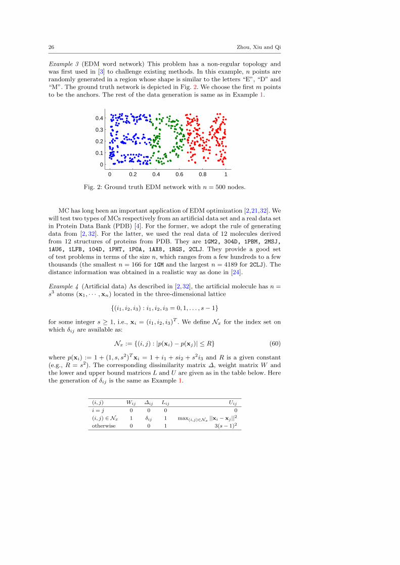
Example 3 (EDM word network) This problem has a non-regular topology andwas first used in [3] to challenge existing methods. In this example, n points arerandomly generated in a region whose shape is similar to the letters “E”, “D” and“M”. The ground truth network is depicted in Fig. 2. We choose the first m pointsto be the anchors. The rest of the data generation is same as in Example 1.
0 0.2 0.4 0.6 0.8 1
0
0.1
0.2
0.3
0.4
Fig. 2: Ground truth EDM network with n = 500 nodes.
MC has long been an important application of EDM optimization [2,21,32]. Wewill test two types of MCs respectively from an artificial data set and a real data setin Protein Data Bank (PDB) [4]. For the former, we adopt the rule of generatingdata from [2, 32]. For the latter, we used the real data of 12 molecules derivedfrom 12 structures of proteins from PDB. They are 1GM2, 304D, 1PBM, 2MSJ,
1AU6, 1LFB, 104D, 1PHT, 1POA, 1AX8, 1RGS, 2CLJ. They provide a good setof test problems in terms of the size n, which ranges from a few hundreds to a fewthousands (the smallest n = 166 for 1GM and the largest n = 4189 for 2CLJ). Thedistance information was obtained in a realistic way as done in [24].
Example 4 (Artificial data) As described in [2,32], the artificial molecule has n =s3 atoms (x1, · · · ,xn) located in the three-dimensional lattice
{(i1, i2, i3) : i1, i2, i3 = 0, 1, . . . , s− 1}
for some integer s ≥ 1, i.e., xi = (i1, i2, i3)T . We define Nx for the index set onwhich δij are available as:
Nx := {(i, j) : |p(xi)− p(xj)| ≤ R} (60)
where p(xi) := 1 + (1, s, s2)Txi = 1 + i1 + si2 + s2i3 and R is a given constant(e.g., R = s2). The corresponding dissimilarity matrix ∆, weight matrix W andthe lower and upper bound matrices L and U are given as in the table below. Herethe generation of δij is the same as Example 1.
(i, j) Wij ∆ij Lij Uij
i = j 0 0 0 0
(i, j) ∈ Nx 1 δij 1 max(i,j)∈Nx||xi − xj ||2
otherwise 0 0 1 3(s− 1)2
Robust Euclidean Embedding 27
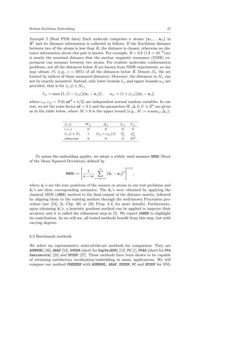
Example 5 (Real PDB data) Each molecule comprises n atoms {x1, . . .xn} in<3 and its distance information is collected as follows. If the Euclidean distancebetween two of the atoms is less than R, the distance is chosen; otherwise no dis-tance information about this pair is known. For example, R = 6A (1A = 10−8cm)is nearly the maximal distance that the nuclear magnetic resonance (NMR) ex-periment can measure between two atoms. For realistic molecular conformationproblems, not all the distances below R are known from NMR experiments, so onemay obtain c% (e.g., c = 50%) of all the distances below R. Denote Nx the setformed by indices of those measured distances. Moreover, the distances in Nx cannot be exactly measured. Instead, only lower bounds `ij and upper bounds uij areprovided, that is for (i, j) ∈ Nx,
`ij = max {1, (1− |εij |)‖xi − xj‖} , uij = (1 + |εij |)‖xi − xj‖.
where εij , εij ∼ N(0, nf2× π/2) are independent normal random variables. In ourtest, we set the noise factor nf = 0.1 and the parameters W,∆,L,U ∈ Sn are givenas in the table below, where M > 0 is the upper bound (e.g., M := nmaxij ∆ij).
(i, j) Wij ∆ij Lij Uij
i = j 0 0 0 0
(i, j) ∈ Nx 1 (`ij + uij)/2 `2ij u2ij
otherwise 0 0 0 M2
To assess the embedding quality, we adopt a widely used measure RMSD (Rootof the Mean Squared Deviation) defined by
RMSD :=
[1
n−m
n∑i=m+1
‖xi − xi‖2]1/2
,
where xi’s are the true positions of the sensors or atoms in our test problems andxi’s are their corresponding estimates. The xi’s were obtained by applying theclassical MDS (cMDS) method to the final output of the distance matrix, followedby aligning them to the existing anchors through the well-known Procrustes pro-cedure (see [53], [6, Chp. 20] or [40, Prop. 4.1] for more details). Furthermore,upon obtaining xi’s, a heuristic gradient method can be applied to improve theiraccuracy and it is called the refinement step in [5]. We report rRMSD to highlightits contribution. As we will see, all tested methods benefit from this step, but withvarying degrees.
6.3 Benchmark methods
We select six representative state-of-the-art methods for comparison. They areADMMSNL [36], ARAP [53], EVEDM (short for EepVecEDM) [12], PC [1], PPAS (short for PPASemismooth) [24] and SFSDP [27]. Those methods have been shown to be capableof returning satisfactory localization/embedding in many applications. We willcompare our method PREEEDM with ADMMSNL, ARAP, EVEDM, PC and SFSDP for SNL

28 Zhou, Xiu and Qi
problems and with EVEDM, PC, PPAS and SFSDP for MC problems since the currentimplementations of ADMMSNL, ARAP do not support the embedding for r ≥ 3.
We note that ADMMSNL is motivated by [44] and aims to enhance the packagediskRelax of [44] for the SNL problems (r = 2). Both methods are based on thestress minimization (5). As we mentioned before, SMACOF [13, 14] has been a verypopular method for (5). However, we are not to compare it with other methods heresince its performance demonstrated in [53,55] was not very satisfactory (e.g., whencomparing with ARAP) for either SNL or MC problems. To our best knowledge, PCis the only viable method, whose code is also publicly available for the model (3).We select SFSDP and PPAS because of their high reputation in the field of SDPand quadratic SDP in returning quality localizations and conformations. We notethat SFSDP is for the model (5) and PPAS is for the model (6). Finally, the methodEVEDM is a latest method for the model (6).
In our tests, we used all of their default parameters except one or two in orderto achieve the best results. In particular, for PC, we terminate it when |f(Dk−1)−f(Dk)| < 10−4 × f(Dk) and set its initial point to be the embedding by cMDS on∆. For SFSDP which is a high-level MATLAB implementation of the SDP approachinitiated in [49], we set pars.SDPsolver = “sedumi” because it returns the bestoverall performance. In addition, we set pars.objSW = 1 when m > r+ 1 and = 3when m = 0. For ARAP, in order to speed up the termination, we let tol = 0.05and IterNum = 20 to compute its local neighbour patches. Numerical performancedemonstrated that ARAP could yield satisfactory embedding, but would take verylong time for some examples with large n.
6.4 Numerical Comparison
In this section, we report our extensive numerical experiments and comparison onthe test data described in Subsect. 6.2. The quality of the general performanceof each method can be better appreciated through visualizing their key indica-tors: RMSD, rRMSD, rTime (time for the refinement step) and the CPU Time (inseconds) which is the total time including rTime. Hereafter, for all examples, wetest 20 randomly generated instances for each case (n,m,R, nf) in SNL or eachcase (n,R, nf) in MC, and record the average results.
6.4.1 Comparison on SNL
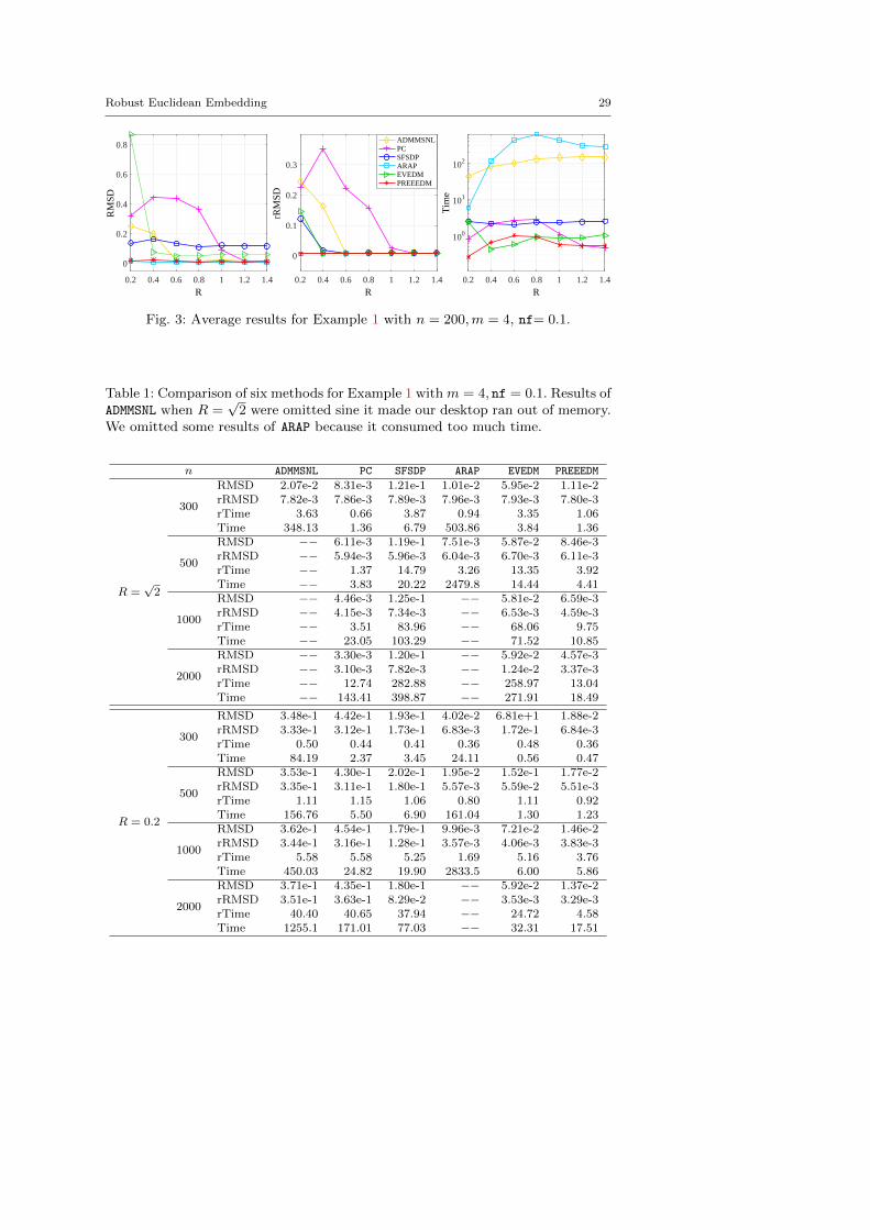
a) Effect of the radio range R. It is easy to see that the radio range R decidesthe amount of missing dissimilarities among all elements of ∆. The smaller R is,the more numbers of δij are unavailable, leading to more challenging problems.Therefore, we first demonstrate the performance of each method to the radio rangeR. For Example 1, we fix n = 200,m = 4, nf= 0.1, and alter the radio range Ramong {0.2, 0.4, · · · , 1.4}. The average results were demonstrated in Figure 3. Itcan be seen that ARAP and PREEEDM were joint winners in terms of both RMSD andrRMSD. However, the time used by ARAP was the longest. When R became biggerthan 0.6, ADMMSNL, SFSDP and EVEDM produced similar rRMSD as ARAP and PREEEDM,while the time consumed by ADMMSNL was significantly larger than that by SFSDP,EVEDM and PREEEDM. By contrast, PC only worked well when R ≥ 1.
Robust Euclidean Embedding 29
0.2 0.4 0.6 0.8 1 1.2 1.4
R
0
0.2
0.4
0.6
0.8
RM
SD
0.2 0.4 0.6 0.8 1 1.2 1.4
R
0
0.1
0.2
0.3
rRM
SD
ADMMSNLPCSFSDPARAPEVEDMPREEEDM
0.2 0.4 0.6 0.8 1 1.2 1.4
R
100
101
102
Tim
e
Fig. 3: Average results for Example 1 with n = 200,m = 4, nf= 0.1.
Table 1: Comparison of six methods for Example 1 with m = 4, nf = 0.1. Results ofADMMSNL when R =
√2 were omitted sine it made our desktop ran out of memory.
We omitted some results of ARAP because it consumed too much time.
n ADMMSNL PC SFSDP ARAP EVEDM PREEEDM
R =√
2
300
RMSD 2.07e-2 8.31e-3 1.21e-1 1.01e-2 5.95e-2 1.11e-2rRMSD 7.82e-3 7.86e-3 7.89e-3 7.96e-3 7.93e-3 7.80e-3rTime 3.63 0.66 3.87 0.94 3.35 1.06Time 348.13 1.36 6.79 503.86 3.84 1.36
500
RMSD −− 6.11e-3 1.19e-1 7.51e-3 5.87e-2 8.46e-3rRMSD −− 5.94e-3 5.96e-3 6.04e-3 6.70e-3 6.11e-3rTime −− 1.37 14.79 3.26 13.35 3.92Time −− 3.83 20.22 2479.8 14.44 4.41
1000
RMSD −− 4.46e-3 1.25e-1 −− 5.81e-2 6.59e-3rRMSD −− 4.15e-3 7.34e-3 −− 6.53e-3 4.59e-3rTime −− 3.51 83.96 −− 68.06 9.75Time −− 23.05 103.29 −− 71.52 10.85
2000
RMSD −− 3.30e-3 1.20e-1 −− 5.92e-2 4.57e-3rRMSD −− 3.10e-3 7.82e-3 −− 1.24e-2 3.37e-3rTime −− 12.74 282.88 −− 258.97 13.04Time −− 143.41 398.87 −− 271.91 18.49
R = 0.2
300
RMSD 3.48e-1 4.42e-1 1.93e-1 4.02e-2 6.81e+1 1.88e-2rRMSD 3.33e-1 3.12e-1 1.73e-1 6.83e-3 1.72e-1 6.84e-3rTime 0.50 0.44 0.41 0.36 0.48 0.36Time 84.19 2.37 3.45 24.11 0.56 0.47
500
RMSD 3.53e-1 4.30e-1 2.02e-1 1.95e-2 1.52e-1 1.77e-2rRMSD 3.35e-1 3.11e-1 1.80e-1 5.57e-3 5.59e-2 5.51e-3rTime 1.11 1.15 1.06 0.80 1.11 0.92Time 156.76 5.50 6.90 161.04 1.30 1.23
1000
RMSD 3.62e-1 4.54e-1 1.79e-1 9.96e-3 7.21e-2 1.46e-2rRMSD 3.44e-1 3.16e-1 1.28e-1 3.57e-3 4.06e-3 3.83e-3rTime 5.58 5.58 5.25 1.69 5.16 3.76Time 450.03 24.82 19.90 2833.5 6.00 5.86
2000
RMSD 3.71e-1 4.35e-1 1.80e-1 −− 5.92e-2 1.37e-2rRMSD 3.51e-1 3.63e-1 8.29e-2 −− 3.53e-3 3.29e-3rTime 40.40 40.65 37.94 −− 24.72 4.58Time 1255.1 171.01 77.03 −− 32.31 17.51

30 Zhou, Xiu and Qi
Next we test a number of instances with larger size n ∈ {300, 500, 1000, 2000}.For Example 1, the average results were recorded in Table 1. When R =
√2 under
which no dissimilarities were missing because Example 1 was generated in a unitregion, PC, ARAP and PREEEDM produced the better RMSD ( almost in the order of10−3). But with the refinement step, all methods led to similar rRMSD. This meantSFSDP and EVEDM benefited a lot from the refinement step. For the computationalspeed, PREEEDM outperformed others, followed by PC, EVEDM and SFSDP. By contrast,ARAP consumed too much time even for n = 500. When R = 0.2, the picture wassignificantly different since there were large amounts of unavailable dissimilaritiesin ∆. Basically, ADMMSNL, PC and SFSDP failed to localize even with the refinementdue to undesirable RMSD and rRMSD (both in the order of 10−1). Clearly, ARAP andPREEEDM produced the best RMSD and rRMSD, and EVEDM got comparable rRMSD butinaccurate RMSD. In terms of the computational speed, EVEDM and PREEEDM werevery fast, consuming about 30 seconds to solve problems with n = 2000 nodes. Bycontrast, ARAP still was the slowest, followed by ADMMSNL and PC.
Table 2: Comparisons of six methods for Example 3 with m = 10, nf = 0.1.
n ADMMSNL PC SFSDP ARAP EVEDM PREEEDM
R =√
1.25
300
RMSD 4.02e-2 5.33e-3 1.45e-1 1.27e-2 1.62e-1 9.26e-3rRMSD 5.12e-3 5.14e-3 5.11e-3 5.12e-3 5.09e-3 5.15e-3rTime 3.28 0.66 3.71 1.69 3.94 1.44Time 346.98 2.00 6.74 553.87 4.42 1.87
500
RMSD −− 4.09e-3 1.07e-1 8.50e-3 1.63e-1 7.15e-3rRMSD −− 4.03e-3 4.04e-3 4.05e-3 1.02e-1 4.15e-3rTime −− 2.68 17.28 7.07 17.39 3.12Time −− 7.24 23.44 2556.3 18.89 5.13
1000
RMSD −− 3.07e-3 1.12e-1 −− 1.28e-1 5.05e-3rRMSD −− 2.98e-3 3.50e-3 −− 4.15e-3 3.15e-3rTime −− 10.35 119.79 −− 122.12 15.73Time −− 43.69 140.66 −− 125.46 20.11
2000
RMSD −− 2.36e-3 1.15e-1 −− 1.03e-1 3.75e-3rRMSD −− 2.28e-3 7.34e-3 −− 7.78e-3 2.26e-3rTime −− 13.43 537.70 −− 489.30 10.59Time −− 238.31 659.71 −− 500.72 20.25
R = 0.1
300
RMSD 1.81e-1 3.77e-1 8.64e-2 8.19e-2 4.06e-1 3.97e-2rRMSD 1.43e-1 1.24e-1 6.69e-2 5.38e-2 1.17e-1 8.21e-3rTime 0.27 0.22 0.21 0.21 0.22 0.21Time 76.57 1.21 3.24 7.24 3.41 0.32
500
RMSD 9.73e-2 3.30e-1 5.08e-2 5.77e-2 2.16e-1 3.63e-2rRMSD 7.82e-2 1.15e-1 3.48e-2 3.08e-2 9.78e-2 3.63e-3rTime 0.67 0.63 0.60 0.58 0.61 0.50Time 148.06 3.63 6.41 50.81 2.07 1.85
1000
RMSD 2.26e-1 3.29e-1 4.80e-2 8.75e-2 2.22e-1 5.01e-2rRMSD 1.01e-1 1.21e-1 9.15e-3 4.55e-2 1.02e-1 2.95e-3rTime 2.74 2.66 2.67 2.58 2.61 2.60Time 353.07 18.01 17.10 842.43 3.22 4.24
2000
RMSD 1.66e-1 3.29e-1 8.21e-2 −− 1.02e-1 5.73e-2rRMSD 1.22e-1 1.53e-1 7.10e-2 −− 3.64e-2 4.97e-3rTime 23.22 23.30 23.06 −− 23.12 17.99Time 887.30 108.81 62.65 −− 26.12 29.89
Robust Euclidean Embedding 31
Now we test those methods for the irregular network in Example 3. The averageresults were recorded in Table 2. We note that no or large numbers of dissimilaritieswere missing when R =
√1.25 and R = 0.1 respectively because this example was
generated in region [0, 1] × [0, 0.5] as presented in Fig. 2. When R =√
1.25, itcan be clearly seen that SFSDP and EVEDM failed to localize before the refinementstep due to their large RMSD (in the order of 10−1), whilst the rest four methodssucceeded. However, they all achieved a similar rRMSD after the refinement exceptfor EVEDM under the case n = 500. Still, PREEEDM ran the fastest and ARAP came thelast, (5.13s vs. 2556.3s when n = 500). Their performances for the case R = 0.1are quite contrasting. We observed that PREEEDM generated the most accurate RMSDand rRMSD (in the order of 10−3) whilst the results of the rest methods were only inthe order of 10−2. Obviously, ADMMSNL, PC and EVEDM failed to localize. Comparedwith the other four methods, EVEDM and PREEEDM were joint winners in terms ofthe computational speed, only using 30s when n = 2000 (a larger scale network).But we should mention that EVEDM failed to localize.
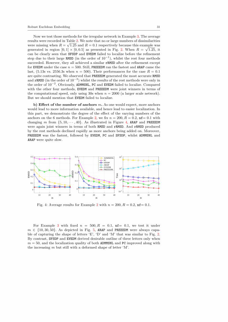
b) Effect of the number of anchors m. As one would expect, more anchorswould lead to more information available, and hence lead to easier localization. Inthis part, we demonstrate the degree of the effect of the varying numbers of theanchors on the 6 methods. For Example 2, we fix n = 200, R = 0.2, nf= 0.1 withchanging m from {5, 10, · · · , 40}. As illustrated in Figure 4, ARAP and PREEEDM
were again joint winners in terms of both RMSD and rRMSD. And rRMSD producedby the rest methods declined rapidly as more anchors being added on. Moreover,PREEEDM was the fastest, followed by EVEDM, PC and SFSDP, whilst ADMMSNL andARAP were quite slow.
10 20 30 40m
0
0.1
0.2
0.3
0.4
0.5
RM
SD
10 20 30 40m
0
0.1
0.2
0.3
0.4
rRM
SD
ADMMSNLPCSFSDPARAPEVEDMPREEEDM
10 20 30 40m
10-1
100
101
102
Tim
e
Fig. 4: Average results for Example 2 with n = 200, R = 0.2, nf= 0.1.
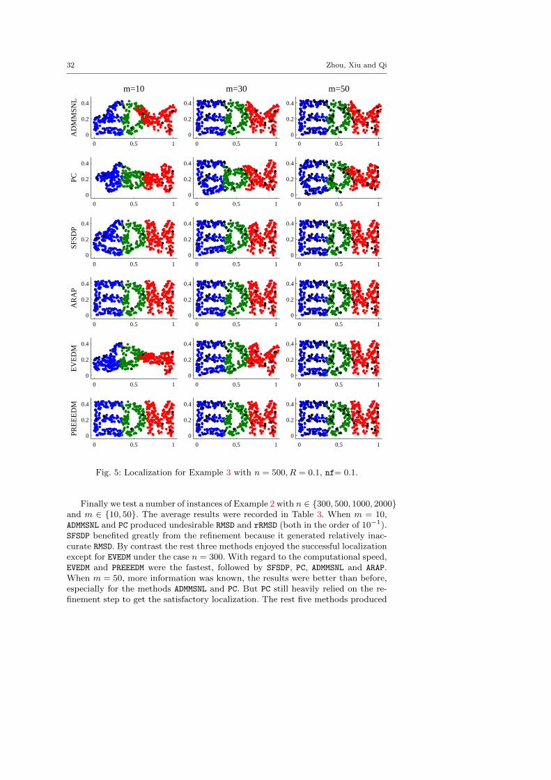
For Example 3 with fixed n = 500, R = 0.1, nf= 0.1, we test it underm ∈ {10, 30, 50}. As depicted in Fig. 5, ARAP and PREEEDM were always capa-ble of capturing the shape of letters ‘E’, ‘D’ and ‘M’ that was similar to Fig. 2.By contrast, SFSDP and EVEDM derived desirable outline of three letters only whenm = 50, and the localization quality of both ADMMSNL and PC improved along withthe increasing m but still with a deformed shape of letter ‘M’.
32 Zhou, Xiu and Qi
0 0.5 1
0
0.2
0.4
AD
MM
SNL
m=10
0 0.5 1
0
0.2
0.4
PC
0 0.5 1
0
0.2
0.4
SFSD
P
0 0.5 1
0
0.2
0.4
AR
AP
0 0.5 1
0
0.2
0.4
EV
ED
M
0 0.5 1
0
0.2
0.4
PRE
EE
DM
0 0.5 1
0
0.2
0.4
m=30
0 0.5 1
0
0.2
0.4
0 0.5 1
0
0.2
0.4
0 0.5 1
0
0.2
0.4
0 0.5 1
0
0.2
0.4
0 0.5 1
0
0.2
0.4
0 0.5 1
0
0.2
0.4
m=50
0 0.5 1
0
0.2
0.4
0 0.5 1
0
0.2
0.4
0 0.5 1
0
0.2
0.4
0 0.5 1
0
0.2
0.4
0 0.5 1
0
0.2
0.4
Fig. 5: Localization for Example 3 with n = 500, R = 0.1, nf= 0.1.
Finally we test a number of instances of Example 2 with n ∈ {300, 500, 1000, 2000}and m ∈ {10, 50}. The average results were recorded in Table 3. When m = 10,ADMMSNL and PC produced undesirable RMSD and rRMSD (both in the order of 10−1).SFSDP benefited greatly from the refinement because it generated relatively inac-curate RMSD. By contrast the rest three methods enjoyed the successful localizationexcept for EVEDM under the case n = 300. With regard to the computational speed,EVEDM and PREEEDM were the fastest, followed by SFSDP, PC, ADMMSNL and ARAP.When m = 50, more information was known, the results were better than before,especially for the methods ADMMSNL and PC. But PC still heavily relied on the re-finement step to get the satisfactory localization. The rest five methods produced
Robust Euclidean Embedding 33
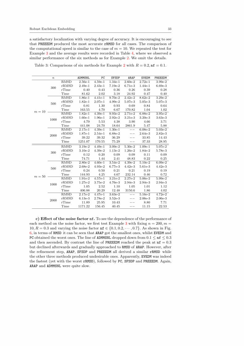
a satisfactory localization with varying degree of accuracy. It is encouraging to seethat PREEEDM produced the most accurate rRMSD for all cases. The comparison ofthe computational speed is similar to the case of m = 10. We repeated the test forExample 3 and the average results were recorded in Table 4, where we observed asimilar performance of the six methods as for Example 2. We omit the details.
Table 3: Comparisons of six methods for Example 2 with R = 0.2, nf = 0.1.
n ADMMSNL PC SFSDP ARAP EVEDM PREEEDM
m = 10
300
RMSD 2.56e-1 4.59e-1 1.34e-1 2.60e-2 2.72e-1 3.99e-2rRMSD 2.49e-1 2.43e-1 7.19e-2 6.71e-3 1.44e-1 6.69e-3rTime 0.40 0.43 0.36 0.26 0.39 0.28Time 81.62 2.02 3.18 24.92 0.47 0.40
500
RMSD 1.86e-1 4.41e-1 9.70e-2 2.42e-2 8.62e-2 3.29e-2rRMSD 1.82e-1 2.07e-1 4.99e-2 5.07e-3 5.05e-3 5.07e-3rTime 0.81 1.30 0.93 0.69 0.84 0.64Time 163.55 4.70 6.67 170.82 1.04 1.02
1000
RMSD 1.82e-1 4.39e-1 9.93e-2 2.71e-2 6.88e-2 3.95e-2rRMSD 1.60e-1 1.96e-1 2.92e-2 3.21e-3 3.20e-3 3.63e-3rTime 4.79 5.53 4.38 3.90 4.66 3.71Time 441.08 24.70 18.64 2861.9 5.47 5.88
2000
RMSD 2.17e-1 4.39e-1 1.30e-1 −− 6.08e-2 5.03e-2rRMSD 1.87e-1 2.54e-1 6.88e-2 −− 2.64e-3 2.82e-3rTime 39.22 39.32 36.29 −− 33.85 14.43Time 1251.07 170.55 75.29 −− 37.33 28.95
m = 50
300
RMSD 3.19e-2 4.49e-1 3.09e-2 5.30e-2 1.09e-1 5.07e-2rRMSD 3.10e-2 4.39e-2 1.13e-2 1.26e-2 1.84e-2 5.78e-3rTime 0.12 0.20 0.09 0.09 0.11 0.09Time 74.71 1.44 2.41 48.83 0.22 0.25
500
RMSD 2.80e-2 4.60e-1 3.54e-2 4.39e-2 5.10e-2 6.09e-2rRMSD 2.68e-2 4.93e-2 6.77e-3 4.42e-3 5.61e-3 4.42e-3rTime 0.24 0.50 0.21 0.21 0.19 0.19Time 144.93 4.25 4.67 232.14 0.46 0.72
1000
RMSD 1.91e-2 4.57e-1 3.21e-2 2.27e-2 5.06e-2 5.99e-2rRMSD 1.27e-2 3.75e-2 4.76e-3 2.94e-3 2.94e-3 2.94e-3rTime 1.05 2.52 1.10 1.05 1.01 1.12Time 406.88 20.29 12.48 3150.6 1.86 4.02
2000
RMSD 2.17e-2 4.47e-1 3.63e-2 −− 5.16e-2 4.72e-2rRMSD 6.13e-3 2.78e-2 3.52e-3 −− 2.06e-3 2.06e-3rTime 11.89 25.95 10.43 −− 8.80 7.71Time 1171.22 156.45 40.45 −− 11.15 22.53
c) Effect of the noise factor nf. To see the dependence of the performance ofeach method on the noise factor, we first test Example 3 with fixing n = 200,m =10, R = 0.3 and varying the noise factor nf ∈ {0.1, 0.2, · · · , 0.7}. As shown in Fig.6, in terms of RMSD it can be seen that ARAP got the smallest ones, whilst EVEDM andPC obtained the worst ones. The line of ADMMSNL dropped down from 0.1 ≤ nf ≤ 0.3and then ascended. By contrast the line of PREEEDM reached the peak at nf = 0.3but declined afterwards and gradually approached to RMSD of ARAP. However, afterthe refinement step, ARAP, SFSDP and PREEEDM all derived a similar rRMSD whilethe other three methods produced undesirable ones. Apparently, EVEDM was indeedthe fastest (yet with the worst rRMSD), followed by PC, SFSDP and PREEEDM. Again,ARAP and ADMMSNL were quite slow.

34 Zhou, Xiu and Qi
Table 4: Comparisons of six methods for Example 3 with R = 0.1, nf = 0.1.
n ADMMSNL PC SFSDP ARAP EVEDM PREEEDM
m = 10
300
RMSD 1.80e-1 3.77e-1 8.86e-2 7.97e-2 3.88e-1 4.05e-2rRMSD 1.48e-1 1.24e-1 6.24e-2 4.51e-2 1.19e-1 6.25e-3rTime 0.28 0.22 0.21 0.22 0.23 0.21Time 76.83 1.12 3.00 7.22 5.92 0.41
500
RMSD 9.71e-2 3.30e-1 4.97e-2 5.97e-2 2.10e-1 3.81e-2rRMSD 8.07e-2 9.98e-2 3.21e-2 3.38e-2 1.04e-1 3.91e-3rTime 0.68 0.59 0.60 0.59 0.59 0.47Time 142.20 3.37 6.35 48.98 2.10 0.98
1000
RMSD 2.30e-1 3.29e-1 4.98e-2 8.86e-2 2.24e-1 4.93e-2rRMSD 1.02e-1 1.18e-1 2.33e-2 4.53e-2 1.07e-1 2.37e-3rTime 2.92 2.84 2.82 2.80 2.85 2.84Time 354.77 18.59 17.43 838.48 3.85 4.55
2000
RMSD 1.66e-1 3.29e-1 7.96e-2 −− 1.03e-1 5.72e-2rRMSD 1.22e-1 1.52e-1 6.92e-2 −− 4.25e-2 4.89e-3rTime 23.24 23.17 23.08 −− 23.05 13.07Time 882.40 98.20 66.58 −− 26.21 24.17
m = 50
300
RMSD 2.24e-2 3.34e-1 1.72e-2 4.04e-2 2.22e-1 3.35e-2rRMSD 2.13e-2 2.44e-2 8.36e-3 1.19e-2 2.11e-2 4.34e-3rTime 0.22 0.21 0.11 0.13 0.22 0.14Time 69.59 0.55 2.30 26.37 0.30 0.29
500
RMSD 2.53e-2 3.41e-1 2.50e-2 4.95e-2 6.14e-2 4.18e-2rRMSD 2.46e-2 3.67e-2 6.64e-3 4.89e-3 2.97e-3 2.96e-3rTime 0.34 0.58 0.42 0.38 0.43 0.37Time 130.58 2.96 5.07 83.65 0.60 0.79
1000
RMSD 1.97e-2 3.30e-1 1.94e-2 4.82e-2 5.60e-2 4.90e-2rRMSD 1.89e-2 3.07e-2 1.95e-3 3.50e-3 1.96e-3 1.96e-3rTime 1.02 2.78 1.04 1.49 1.36 1.23Time 314.30 14.31 12.87 947.29 1.97 3.48
2000
RMSD 4.64e-3 3.28e-1 2.10e-2 −− 6.30e-2 5.72e-2rRMSD 1.32e-3 3.01e-2 1.32e-3 −− 1.32e-3 1.32e-3rTime 14.59 23.23 13.03 −− 13.87 8.28Time 811.23 99.02 44.12 −− 15.99 19.45
0.1 0.2 0.3 0.4 0.5 0.6 0.7
nf
0
0.1
0.2
0.3
0.4
RM
SD
0.1 0.2 0.3 0.4 0.5 0.6 0.7
nf
0
0.05
0.1
0.15
0.2
rRM
SD
ADMMSNLPCSFSDPARAPEVEDMPREEEDM
0.1 0.2 0.3 0.4 0.5 0.6 0.7
nf
100
101
102
Tim
e
Fig. 6: Average results for Example 3 with n = 200,m = 10, R = 0.3.
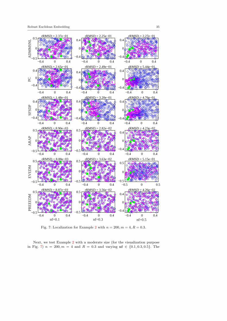
Robust Euclidean Embedding 35
−0.4 0 0.4−0.5
0
0.5
AD
MM
SNL
rRMSD = 2.37e−01
−0.4 0 0.4
−0.4
0
0.4
PC
rRMSD = 2.65e−01
−0.4 0 0.4
−0.4
0
0.4
SFSD
P
rRMSD = 1.48e−01
−0.4 0 0.4−0.5
0
0.5
AR
AP
rRMSD = 8.90e−03
−0.4 0 0.4−0.5
0
0.5
EV
ED
M
rRMSD = 8.88e−03
−0.4 0 0.4−0.5
0
0.5
nf=0.1
PRE
EE
DM
rRMSD = 8.87e−03
−0.4 0 0.4
−0.4
0
0.4rRMSD = 2.25e−01
−0.4 0 0.4
−0.4
0
0.4
rRMSD = 2.49e−01
−0.4 0 0.4
−0.4
0
0.4rRMSD = 3.20e−01
−0.4 0 0.4−0.5
0
0.5rRMSD = 2.82e−02
−0.4 0 0.4−0.5
0
0.5rRMSD = 3.63e−02
−0.4 0 0.4−0.5
0
0.5
nf=0.3
rRMSD = 3.56e−02
−0.4 0 0.4
−0.4
0
0.4rRMSD = 2.27e−01
−0.4 0 0.4
−0.4
0
0.4rRMSD = 5.44e−01
−0.4 0 0.4
−0.4
0
0.4rRMSD = 4.76e−01
−0.4 0 0.4
−0.4
0
0.4rRMSD = 4.23e−02
−0.5 0 0.5−0.5
0
0.5rRMSD = 5.15e−01
−0.4 0 0.4
−0.4
0
0.4
nf=0.5
rRMSD = 4.26e−02
Fig. 7: Localization for Example 2 with n = 200,m = 4, R = 0.3.
Next, we test Example 2 with a moderate size (for the visualization purposein Fig. 7) n = 200,m = 4 and R = 0.3 and varying nf ∈ {0.1, 0.3, 0.5}. The
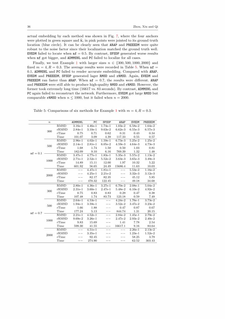
36 Zhou, Xiu and Qi
actual embedding by each method was shown in Fig. 7, where the four anchorswere plotted in green square and xi in pink points were jointed to its ground truthlocation (blue circle). It can be clearly seen that ARAP and PREEEDM were quiterobust to the noise factor since their localization matched the ground truth well.EVEDM failed to locate when nf = 0.5. By contrast, SFSDP generated worse resultswhen nf got bigger, and ADMMSNL and PC failed to localize for all cases.
Finally, we test Example 1 with larger sizes n ∈ {300, 500, 1000, 2000} andfixed m = 4, R = 0.3. The average results were recorded in Table 5. When nf =0.1, ADMMSNL and PC failed to render accurate embedding. Compared with ARAP,EVEDM and PREEEDM, SFSDP generated lager RMSD and rRMSD. Again, EVEDM andPREEEDM ran faster than ARAP. When nf = 0.7, the results were different. ARAP
and PREEEDM were still able to produce high-quality RMSD and rRMSD. However, theformer took extremely long time (16617 vs. 83 seconds). By contrast, ADMMSNL andPC again failed to reconstruct the network. Furthermore, EVEDM got large RMSD butcomparable rRMSD when n ≤ 1000, but it failed when n = 2000.
Table 5: Comparisons of six methods for Example 1 with m = 4, R = 0.3.
n ADMMSNL PC SFSDP ARAP EVEDM PREEEDM
nf = 0.1
300
RMSD 3.16e-1 4.46e-1 1.74e-1 1.03e-2 6.58e-2 1.64e-2rRMSD 2.84e-1 3.10e-1 9.63e-2 6.62e-3 6.55e-3 6.57e-3rTime 0.75 0.71 0.62 0.31 0.43 0.34Time 101.07 3.09 4.39 117.33 0.55 0.57
500
RMSD 2.96e-1 4.02e-1 1.59e-1 6.73e-3 5.25e-2 1.25e-2rRMSD 2.14e-1 2.81e-1 6.05e-2 4.59e-3 4.64e-3 4.73e-3rTime 1.68 1.74 1.50 0.50 1.03 0.81Time 182.09 9.10 6.16 769.39 1.32 1.48
1000
RMSD 3.47e-1 4.77e-1 1.83e-1 5.35e-3 5.57e-2 1.13e-2rRMSD 2.71e-1 2.52e-1 5.52e-2 3.63e-3 3.65e-3 3.49e-3rTime 14.89 15.11 12.00 1.97 10.32 5.22Time 601.92 56.65 24.49 15686.4 11.63 10.03
2000
RMSD −− 4.47e-1 1.81e-1 −− 5.53e-2 1.16e-2rRMSD −− 4.25e-1 2.21e-2 −− 3.32e-3 3.12e-3rTime −− 82.17 82.35 −− 45.12 5.85Time −− 470.32 122.45 −− 49.18 34.68
nf = 0.7
300
RMSD 2.80e-1 4.36e-1 3.27e-1 6.70e-2 2.08e-1 5.04e-2rRMSD 2.31e-1 3.60e-1 2.47e-1 5.48e-2 6.10e-2 4.92e-2rTime 0.75 0.83 0.83 0.29 0.47 0.38Time 107.48 1.74 83.73 123.18 0.59 7.49
500
RMSD 2.64e-1 4.53e-1 −− 4.24e-2 1.76e-1 3.73e-2rRMSD 1.94e-1 3.59e-1 −− 3.52e-2 3.47e-2 3.23e-2rTime 1.66 1.88 −− 0.47 0.87 0.67Time 177.24 5.13 −− 844.74 1.31 20.15
1000
RMSD 2.21e-1 4.52e-1 −− 2.84e-2 1.45e-1 2.79e-2rRMSD 9.69e-2 3.26e-1 −− 2.47e-2 2.93e-2 2.40e-2rTime 9.83 15.69 −− 1.41 7.78 2.54Time 599.30 41.55 −− 16617.1 9.16 83.64
2000
RMSD −− 4.51e-1 −− −− 2.26e-1 2.13e-2rRMSD −− 3.35e-1 −− −− 1.23e-1 1.52e-2rTime −− 92.45 −− −− 58.25 3.79Time −− 274.90 −− −− 62.52 303.43
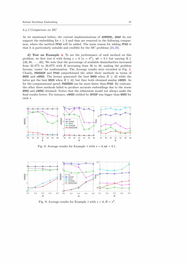
Robust Euclidean Embedding 37
6.4.2 Comparison on MC
As we mentioned before, the current implementations of ADMMSNL, ARAP do notsupport the embedding for r ≥ 3 and thus are removed in the following compar-ison, where the method PPAS will be added. The main reason for adding PPAS isthat it is particularly suitable and credible for the MC problems [24,25].
d) Test on Example 4. To see the performance of each method on thisproblem, we first test it with fixing s = 6 (n = 63), nf = 0.1 but varying R ∈{36, 38, · · · , 48}. We note that the percentage of available dissimilarities increasedfrom 32.47% to 39.87% with R increasing from 36 to 48, making the problembecome ‘easier’ for conformation. The Average results were recorded in Fig. 8.Clearly, PREEEDM and PPAS outperformed the other three methods in terms ofRMSD and rRMSD. The former generated the best RMSD when R ≥ 42 while thelatter got the best RMSD when R ≤ 42, but they both obtained similar rRMSD. Asfor the computational speed, PREEEDM ran far more faster than PPAS. By contrast,the other three methods failed to produce accurate embeddings due to the worseRMSD and rRMSD obtained. Notice that the refinement would not always make thefinal results better. For instance, rRMSD yielded by SFSDP was bigger than RMSD foreach s.
36 38 40 42 44 46 48
R
0
1
2
3
RM
SD
36 38 40 42 44 46 48
R
0
1
2
3
4
rRM
SD PCSFSDPPPASEVEDMPREEEDM
36 38 40 42 44 46 48
R
100
101
Tim
e
Fig. 8: Average results for Example 4 with s = 6, nf = 0.1.
0.1 0.2 0.3 0.4 0.5
nf
0
1
2
3
RM
SD
0.1 0.2 0.3 0.4 0.5
nf
0
1
2
3
4
rRM
SD PCSFSDPPPASEVEDMPREEEDM
0.1 0.2 0.3 0.4 0.5
nf
100
101
102
Tim
e
Fig. 9: Average results for Example 4 with s = 6, R = s2.

38 Zhou, Xiu and Qi
We then test the example with fixing s = 6 (n = 63), R = s2 and varyingnf ∈ {0.1, 0.2, · · · , 0.5}. As illustrated in Fig. 9, in terms of RMSD and rRMSD, itcan be clearly seen that PREEEDM and PPAS were the joint winners. In particular,our method rendered the best RMSD when nf ≥ 0.2 and also ran much faster thanPPAS. Obviously, the other three methods again failed to obtain desirable RMSD andrRMSD irrelevant of the time they used.
Finally, for larger size problems with n = s3 and s ∈ {7, 8, . . . , 13}, the averageresults were presented in Fig. 10, where we omitted the results by PPAS for s > 10because it took too much time to terminate. It is worth mentioning that thepercentage of the available dissimilarities over all elements of ∆ decreases from26.78% to 14.83% when s increasing from 7 to 13, making the problems moreand more challenging. Clearly PC, SFSDP and EVEDM failed to locate all atoms in<3. PPAS rendered the most accurate RMSD when s ≤ 10 whilst PREEEDM achievedthe most accurate RMSD when s > 10 and the most accurate rRMSD for all cases.Equally important for PREEEDM is that it spent less than 50 seconds for all testedcases, while PPAS took much more time to terminate (e.g., consuming over 2000seconds when s ≥ 10).
7 8 9 10 11 12 13
s
0
1
2
3
4
5
6
RM
SD
7 8 9 10 11 12 13
s
0
2
4
6
8
rRM
SD
PCSFSDPPPASEVEDMPREEEDM
7 8 9 10 11 12 13
s
101
102
103
Tim
e
Fig. 10: Average results for Example 4 with n = s3, R = s2, nf = 0.1.
e) Test on Example 5. For the 12 collected real data, we fixed R = 6, c =50% and nf = 0.1. The generated embeddings by the five methods for the threemolecules 1GM2, 1AU6 and 1LFB were shown in Fig. 11, where the true and estimatedpositions of the atoms were plotted by blue circles and pink stars respectively. Eachpink star was linked to its corresponding blue circle by a pink line. For these threedata, PREEEDM and PPAS almost conformed the shape of the original data. Clearly,the other three methods failed to conform. The complete numerical results for the12 problems were reported in Table 6. It can be clearly seen that PREEEDM andPPAS performed significantly better in terms of the RMSD and rRMSD than the othermethods. What is more impressive is that PREEEDM only used a small fraction ofthe time by PPAS, which in general took relatively long time to terminate. Forexample, PREEEDM only used 22.64 seconds for 2CLJ, which is a very large data setwith n = 4189. In contrast, we had to omit the result of PPAS for this instance (aswell as to omit for other tested instances, and the missed results were indicatedas “−−” in Table 6) because it took too long to terminate.
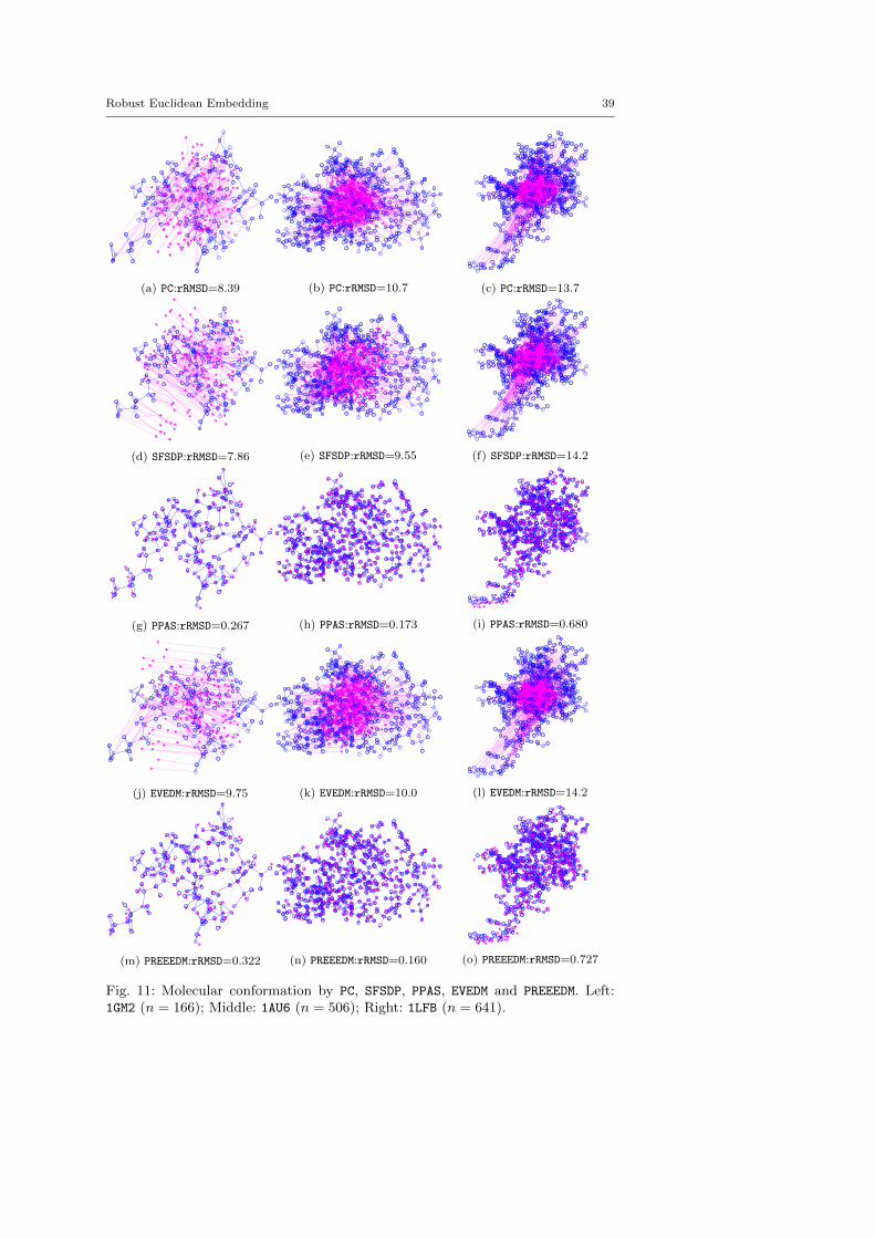
Robust Euclidean Embedding 39
(a) PC:rRMSD=8.39 (b) PC:rRMSD=10.7 (c) PC:rRMSD=13.7
(d) SFSDP:rRMSD=7.86 (e) SFSDP:rRMSD=9.55 (f) SFSDP:rRMSD=14.2
(g) PPAS:rRMSD=0.267 (h) PPAS:rRMSD=0.173 (i) PPAS:rRMSD=0.680
(j) EVEDM:rRMSD=9.75 (k) EVEDM:rRMSD=10.0 (l) EVEDM:rRMSD=14.2
(m) PREEEDM:rRMSD=0.322 (n) PREEEDM:rRMSD=0.160 (o) PREEEDM:rRMSD=0.727
Fig. 11: Molecular conformation by PC, SFSDP, PPAS, EVEDM and PREEEDM. Left:1GM2 (n = 166); Middle: 1AU6 (n = 506); Right: 1LFB (n = 641).

40 Zhou, Xiu and Qi
Table 6: Comparisons of the five methods for Example 5.
PC SFSDP PPAS EVEDM PREEEDM
RMSD 6.60e+0 6.65e+0 4.07e-1 6.51e+0 9.09e-11GM2 rRMSD 7.07e+0 6.92e+0 2.65e-1 7.41e+0 3.51e-1n = 166 rTime 0.17 0.18 0.22 0.18 0.16
Time 0.98 4.84 15.43 0.98 0.27
RMSD 1.03e+1 1.03e+1 2.89e+0 1.02e+1 3.61e+0304D rRMSD 1.07e+1 1.08e+1 1.43e+0 1.08e+1 2.50e+0n = 237 rTime 0.16 0.16 0.55 0.16 0.15
Time 1.07 7.76 36.44 1.36 0.23
RMSD 8.45e+0 8.47e+0 5.29e-1 8.35e+0 1.23e+01PBM rRMSD 9.13e+0 8.91e+0 2.01e-1 9.28e+0 2.11e-1n = 388 rTime 0.51 0.49 0.53 0.49 0.32
Time 2.84 28.64 112.82 1.45 0.54
RMSD 1.06e+1 1.06e+1 5.40e-1 1.05e+1 9.15e-12MSJ rRMSD 1.12e+1 1.11e+1 2.99e-1 1.10e+1 3.34e-1n = 480 rTime 0.40 0.39 0.54 0.39 0.32
Time 2.32 118.60 196.12 1.47 0.59
RMSD 9.30e+0 9.31e+0 4.02e-1 9.20e+0 6.74e-11AU6 rRMSD 9.99e+0 9.83e+0 1.68e-1 9.69e+0 1.63e-1n = 506 rTime 0.70 0.68 0.30 0.69 0.35
Time 4.12 47.68 262.28 1.47 0.70
RMSD 1.34e+1 1.34e+1 1.56e+0 1.33e+1 1.57e+01LFB rRMSD 1.39e+1 1.35e+1 5.41e-1 1.37e+1 7.38e-1n = 641 rTime 0.49 0.49 1.63 0.48 0.37
Time 2.93 132.96 956.44 1.64 0.79
RMSD 1.23e+1 1.23e+1 4.30e+0 1.22e+1 3.27e+0104D rRMSD 1.27e+1 1.27e+1 2.02e+0 1.26e+1 1.26e+0n = 766 rTime 0.89 0.86 3.40 0.87 0.61
Time 5.04 72.16 2024.51 1.47 1.40
RMSD 1.23e+1 1.23e+1 1.70e+0 1.23e+1 1.58e+01PHT rRMSD 1.29e+1 1.26e+1 9.16e-1 1.26e+1 9.85e-1n = 814 rTime 0.74 0.74 2.57 0.74 0.48
Time 4.86 411.14 4726.96 1.71 1.25
RMSD 1.42e+1 1.42e+1 1.39e+0 1.41e+1 1.48e+01POA rRMSD 1.45e+1 1.46e+1 3.27e-1 1.46e+1 4.51e-1n = 914 rTime 0.58 0.55 1.34 0.55 0.52
Time 5.03 587.14 1623.43 1.99 1.45
RMSD 1.43e+1 1.43e+1 −− 1.43e+1 1.23e+01AX8 rRMSD 1.47e+1 1.45e+1 −− 1.44e+1 5.01e-1n = 1003 rTime 0.62 0.58 −− 0.59 0.34
Time 5.78 1404.53 −− 1.54 1.49
RMSD 2.02e+1 −− −− 2.02e+1 1.99e+01RGS rRMSD 2.05e+1 −− −− 2.06e+1 6.76e-1n = 2015 rTime 1.33 −− −− 1.25 0.94
Time 16.08 −− −− 3.69 5.71
RMSD 2.27e+1 −− −− 2.27e+1 1.54e+02CLJ rRMSD 2.30e+1 −− −− 2.29e+1 6.50e-1n = 4189 rTime 4.46 −− −− 3.82 2.35
Time 43.10 −− −− 378.35 22.64
Robust Euclidean Embedding 41
7 Conclusion
The purpose of this paper is to develop an efficient method for one of the mostchallenging distance embedding problems in a low-dimensional space, which havebeen widely studied under the framework of multi-dimensional scaling. The prob-lem employs `1 norm to quantify the embedding errors. Hence, the resulting model(3) appears to be robust to outliers and is referred to as the robust Euclidean em-bedding (REE) model.
To the best knowledge of the authors, the only viable method, whose matlabcode is also publicly available for REE is the PlaceCenter (PC) algorithm proposedin [1]. Our extensive numerical results on the SNL and MC test problems convinc-ingly demonstrated that the proposed PREEEDM method outperform PC in termsof both the embedding quality and the CPU time. Moreover, PREEEDM is also com-parable to several state-of-the-art methods for other embedding models in termsof the embedding quality, but is far more efficient in terms of the CPU time. Theadvantage becomes even more superior as the size of the problem gets bigger.
The novelty of the proposed PREEEDM lies with its creative use of the Euclideandistance matrix and a computationally efficient majorization technique to deriveits subproblem, which has a closed-form solution closely related to the positiveroot of the classical depressed cubic equation. Furthermore, a great deal of efforthas been devoted to its convergence analysis, which well justifies the numericalperformance of PREEEDM. We feel that PREEEDM will become a very competitiveembedding method in the field of SNL and MC and expect its wide use in othervisualization problems.
Acknowledgements We thank Mr Nicola Piovsan and Prof Nathan Krislock respectivelyfor sharing with us their excellent packages ADMMSNL and EepVecEDM. In particular, we thankProf Kim-Chuan Toh for his encouragement over the past years in algorithmic implementation,acquiring PDB data and for sharing with us his well-structured package PPAS. This work ispartly supported by the National Science Foundation of China (11728101, 71611130218).
References
1. A. Agarwal, J.M. Phillips and S. Venkatasubramanian, Universal multi-dimensional scaling,In Proceedings of the 16th ACM SIGKDD international conference on Knowledge discoveryand data mining, pp. 1149-1158, ACM, 2010.
2. LTH An and PD Tao, Large-scale molecular optimization from distance matrices by a dcoptimization approach, SIAM J. Optim. 14 (2003), pp. 77–114.
3. S. Bai and H.-D. Qi, Tackling the flip ambiguity in wireless sensor network localizationand beyond, Digital Signal Process., 55 (2016), pp. 85-97.
4. H.M. Berman, J. Westbrook, Z. Feng, G. Gillilan, T.N. Bhat, H. Weissig, I.N. Shindyalovand P.E. Bourne, “The protein data bank”, Nucleic Acids Res. 28, pp. 235242, 2000.
5. P. Biswas, T.-C. Liang, K.-C. Toh, T.-C. Wang and Y. Ye, Semidefinite programmingapproaches for sensor network localization with noisy distance measurements, IEEE Trans.Auto. Sci. Eng., 3, pp. 360-371, 2006.
6. I. Borg and P.J.F. Groenen, Modern Multidimensional Scaling: Theory and Applications,2nd Ed., Springer Series in Statistics, Springer, 2005.
7. D.M. Burton, The History of Mathematics (7th Eds), MaGraw-Hill, 2011.8. L. Cayton and S. Dasgupta Robust Euclidean embedding, Proceedings of the 23rd Inter-
national Conference on Machine Learning, Pittsburgh, PA 2006, pp. 169–176.9. Y.Q. Chen, N.H. Xiu and D.T. Peng, Global solutions of non-Lipschitz S2Sp minimiza-
tion over the positive semidefinite cone, Optimization Letters, 8 (2014), pp. 2053-2064.

42 Zhou, Xiu and Qi
10. T.F. Cox and M.A.A. Cox, Multidimensional Scaling, 2nd Ed, Chapman and Hall/CRC,2001.
11. C. Ding and H.-D. Qi, Convex optimization learning of faithful Euclidean distance repre-sentations in nonlinear dimensionality reduction, Math. Program., 164 (2017), pp. 341-381.
12. D. Drusvyatskiy, N. Krislock, Y.L. Voronin and H. Wolkowicz, Noisy Euclideandistance realization: robust facial reduction and the Pareto frontier, SIAM Journal on Op-timization, 27(4), 2301-2331, 2017.
13. J. de Leeuw, Applications of Convex Analysis to Multidimensional Scaling, In J Barra, FBrodeau, G Romier, B van Cutsem (eds.), Recent Developments in Statistics, pp. 133–145.North Holland Publishing Company, Amsterdam, The Netherlands, 1977.
14. J. de Leeuw and P. Mair, Multidimensional scaling using majorization: Smacof in R,J. Stat. Software, 31, pp. 1-30, 2009.
15. P. Biswas and Y. Ye, Semidefinite programming for ad hoc wireless sensor networklocalization, in Proceedings of the 3rd IPSN, Berkeley, CA, pp. 46-54, 2004.
16. D. Drusvyatskiy, N. Krislock, Y.-L. Voronin and H. Wolkowicz, Noisy Euclideandistance realization: Robust facial reduction and the Pareto frontier, SIAM J. Optim.,27(2017), 2301–2331.
17. S.L. France and J.D. Carroll, Two-way multidimensional scaling: a review, IEEETrans. Syst. Man, and Cyber. – Part C, 41 (2011), pp. 644-661.
18. Y. Gao, Structured Low Rank Matrix Optimization Problems: a Penalty Approach, PhDThesis, National University of Singapore, 2010.
19. N. Gaffke and R. Mathar, A cyclic projection algorithm via duality, Metrika, 36 (1989),pp. 29-54.
20. W. Glunt, T.L. Hayden, S. Hong and J. Wells, An alternating projection algorithmfor computing the nearest Euclidean distance matrix, SIAM J. Matrix Anal. Appl., 11 (1990),pp. 589-600.
21. W. Glunt, T.L. Hayden and R. Raydan, Molecular conformations from distance ma-trices, J. Comput. Chemistry, 14 (1993), pp. 114-120.
22. J.C. Gower 1966, Some distance properties of latent root and vector methods used inmultivariate analysis, Biometrika 53 (1966), pp. 325–338.
23. W.J. Heiser, Multidimensional scaling with least absolute residuals, in Proceedings of theFirst Conference of the International Federation of Classification Societies (IFCS), Aachen,Germany, June 1987, pp. 455-462.
24. K.F. Jiang, D.F Sun and K.C. Toh, Solving nuclear norm regularized and semidefi-nite matrix least squares problems with linear equality constraints, Discrete Geometry andOptimization, Springer International Publishing, pp. 133-162, 2013.
25. K.F. Jiang, D.F. Sun and K.-C. Toh, A partial proximal point algorithm for nuclearnorm regularized matrix least squares problems, Math. Programming Comput., 6 (2014),281–325.
26. C. Kanzow and H.-D. Qi, A QP-free constrained Newton-type method for variationalinequality problems, Math. Prog., 85 (1999), pp. 81-106.
27. S. Kim, M. Kojima, H. Waki and M. Yamashita, Algorithm 920: SFSDP: A sparseversion of full semidefinite programming relaxation for sensor network localization problems,ACM Trans. Math. Softw., 38(4), pp. 27:1-27:19, 2012.
28. S. Korkmaz and A.J. Van der Veen, Robust localization in sensor networks with itera-tive majorization techniques, ICASSP, 2009, pp. 2049-2052.
29. J.B. Kruskal, Nonmetric multidimensional scaling: a numerical method, Psychometrika,29 (1964), pp. 115-129.
30. F.D. Mandanas and C.L. Kotropoulos, Robust multidimensional scaling using a max-imum correntropy criterion, IEEE Trans. Signal Process., 65 (2017), pp. 919–932.
31. C.A. Micchelli, Interpolation of scattered data: distance matrices and conditionally pos-itive definite functinos, Constr. Approx., 2 (1986), pp. 11-22.
32. J.J. More and Z. Wu, Global continuation for distance geometry problems, SIAM J. Op-tim., 7, pp. 814836, 1997.
33. G. Nocedal and S.J. Wright, Numerical Optimization (2nd Eds), Springer, 2006.34. P. Oguz-Ekim, J.P. Gomes, J. Xavier and P. Oliveira, Robust localization of nodes and
time-recursive tracking in sensor networks using noisy range measurements, IEEE Trans.Signal Process., 59 (2011), pp. 3930-3942.
35. D.T Peng, N.H. Xiu and J. Yu, S1/2 regularization methods and fixed point algorithmsfor affine rank minimization problems, Comput. Optim. Appl., 67 (2017), pp. 543–569.

Robust Euclidean Embedding 43
36. N. Piovesan and T. Erseghe, Cooperative localization in WSNs: a hybrid convex/non-convex solution, IEEE Trans. Signal and Information Processing over Networks, DOI10.1109/TSIPN.2016.2639442 (IEEE early access article, 2016).
37. T.K. Pong, Edge-based semidefinite programming relaxation of sensor network localiza-tion with lower bound constraints, Comput Optim Appl., 53, pp. 23-44, 2012.
38. H.-D. Qi, A semismooth Newton method for the nearest Euclidean distance matrix prob-lem, SIAM J. Matrix Anal. Appl. 34 (2013), pp. 67-93.
39. H.-D. Qi and X.M. Yuan, Computing the nearest Euclidean distance matrix with lowembedding dimensions, Math. Prog., 147 (2014), pp. 351-389.
40. H.-D. Qi, N.H. Xiu, and X.M. Yuan, A Lagrangian dual approach to the single sourcelocalization problem, IEEE Trans. Signal Process., 61, pp. 3815-3826, 2013.
41. R.T. Rockafella and R. J-B Wets, Variational Analysis (3rd Eds), Springer, 2009.42. I.J. Schoenberg, Remarks to Maurice Frechet’s article Sur la definition axiomatque d’une
classe d’espaces vectoriels distancies applicbles vectoriellement sur l’espace de Hilbet, Ann.Math., 36 (1935), pp. 724-732.
43. Y. Shang, W. Ruml, Y. Zhang and M.P.J. Fromherz, Localization from mere connectiv-ity, in: Proceedings of the 4th ACM International Symposium on Mobile Ad Hoc Networking& Computing, MobiHoc 03, ACM, New York, NY, USA, pp. 201-212, 2003.
44. C. Soares, J. Xavier and J. Gomes, Simple and fast convex relaxation method for coopera-tive localization in sensor networks using range measurements, IEEE Trans. Signal Process.,63(17), pp. 4532-4543, 2015.
45. Y. Sun, P. Babu and D.P. Palomar, Majorization-minimization algorithms in signalprocessing, communications, and machine learning, IEEE Trans. Signal Process., 65 (2017),pp. 794-816.
46. J.B. Tenenbaum, V. de Silva and J.C. Langford, A global geometric framework fornonlinear dimensionality reduction, Science, 290 (2000), pp. 2319-2323.
47. K.C. Toh, An inexact path-following algorithm for convex quadratic SDP, Math. Prog.,112 (2008), pp. 221254.
48. W.S. Torgerson, Multidimensional scaling: I. Theory and method, Psychometrika, 17(1952), pp. 401-419.
49. Z. Wang, S. Zheng, Y. Ye and S. Boyd, Further relaxations of the semidefinite pro-gramming approach to sensor network localization, SIAM J. Optim., 19 (2008), pp. 655-673.
50. F.C. Xing, Investigation on solutions of cubic equations with one unknown, J. CentralUniv. Nat. (Natural Sci. Ed.), 12 (2003), pp. 207-218.
51. Z. Xu, X. Chang, F. Xu and H. Zhang, L1/2 regularization: a thresholding representationtheory and a fast solver, IEEE Trans. Neural Netw. Learn. Sys., 23 (2012), pp. 1013-1027.
52. G. Young and A.S. Householder, Discussion of a set of points in terms of their mutualdistances, Psychometrika, 3 (1938), pp. 19-22.
53. L. Zhang, L. Liu, C. Gotsman and S.J. Gortler, An as-rigid-as-possible approach tosensor network localization, ACM Trans. Sen. Netw., 6 (2010), pp. 35:1-35:21.
54. L. Zhang, G. Wahba and M. Yuan, Distance shrinkage and Euclidean embedding viaregularized kernel estimation, J. Royal Stat. Soc.: Series B, 78 (2016), pp. 849-867.
55. S.L. Zhou, N.H. Xiu and H.D. Qi, A fast matrix majorization-projection method for constrained stress minimization in MDS, available athttps://www.researchgate.net/publication/319128036, 2017.