arX

iv:1

207.

4831

v3 [

mat

h.O

C]

26 M

ay 2

013

1

Robust Energy Management for MicrogridsWith High-Penetration Renewables

Yu Zhang,Student Member, IEEE,Nikolaos Gatsis,Member, IEEE,and Georgios B. Giannakis,Fellow, IEEE

Abstract—Due to its reduced communication overhead androbustness to failures, distributed energy management is ofparamount importance in smart grids, especially in microgrids,which feature distributed generation (DG) and distributed stor-age (DS). Distributed economic dispatch for a microgrid with highrenewable energy penetration and demand-side managementoperating in grid-connected mode is considered in this paper.To address the intrinsically stochastic availability of renewableenergy sources (RES), a novel power scheduling approach isintroduced. The approach involves the actual renewable energy aswell as the energy traded with the main grid, so that the supply-demand balance is maintained. The optimal scheduling strategyminimizes the microgrid net cost, which includes DG and DScosts, utility of dispatchable loads, and worst-case transactioncost stemming from the uncertainty in RES. Leveraging the dualdecomposition, the optimization problem formulated is solvedin a distributed fashion by the local controllers of DG, DS, anddispatchable loads. Numerical results are reported to corroboratethe effectiveness of the novel approach.

Index Terms—Demand side management, distributed algo-rithms, distributed energy resources, economic dispatch,energymanagement, microgrids, renewable energy, robust optimization.

NOMENCLATURE

A. Indices, numbers, and sets

T , t Number of scheduling periods, period index.M , m Number of conventional distributed generation

(DG) units, and their index.N , n Number of dispatchable (class-1) loads, load in-

dex.Q, q Number of energy (class-2) loads, load index.J , j Number of distributed storage (DS) units, and their

index.I, i Number of power production facilities with renew-

able energy source (RES), and facility index.S, s Number of sub-horizons, and sub-horizon index.k Algorithm iteration index.T Set of time periods in the scheduling horizon.Ts Sub-horizons for all RES facilities.Ti,s Sub-horizons for RES facility i.M Set of conventional DG units.N Set of dispatchable loads.Q Set of energy loads.

This work was supported by the University of Minnesota Institute ofRenewable Energy and the Environment (IREE) under Grant RL-0010-13.This work was presented in part at the3rd IEEE Intl. Conf. on Smart GridCommun., Tainan, Taiwan, November 5–8, 2012.

The authors are with the Dept. of ECE and the Digital Technology Center,University of Minnesota, Minneapolis, MN 55455, USA. Tel/fax: +1(612)624-9510/625-2002. E-mails:{zhan1220,gatsisn,georgios}@umn.edu

J Set of DS units.W Power output uncertainty set for all RES facilities.Wi Power output uncertainty set of RES facilityi.

B. Constants

PminGm

, PmaxGm

Minimum and maximum power output ofconventional DG unitm.

Rm,up, Rm,down Ramp-up and ramp-down limits of con-ventional DG unitm.

SRt Spinning reserve for conventional DG.

Lt Fixed power demand of critical loads inperiodt.

PminDn

, PmaxDn

Minimum and maximum power consump-tion of loadn.

Pmin,tEq

, Pmax,tEq

Minimum and maximum power consump-tion of loadq in periodt.

Sq, Tq Power consumption start and stop timesof load q.

Emaxq Total energy consumption of loadq from

start timeSq to termination timeTq.PminBj

, PmaxBj

Minimum and maximum (dis)chargingpower of DS unitj.

Bminj Minimum stored energy of DS unitj in

periodT .Bmax

j Capacity of DS unitj.ηj Efficiency of DS unitj.PminR , Pmax

R Lower and upper bounds forP tR.

W ti, W

t

i Minimum and maximum forecastedpower output of RES facilityi in t.

Wmini,s , Wmax

i,s Minimum and maximum forecasted totalwind power of wind farmi across sub-horizonTi,s.

Wmins , Wmax

s Minimum and maximum forecasted totalwind power of all wind farms across sub-horizonTs.

αt, βt; γt, δt Purchase and selling prices; and functionsthereof.

πtq Parameter of utility function of loadq.

DODj ; ψtj Depth of discharge specification of DS

unit j; and parameters of storage cost.

C. Uncertain quantities

W ti Power output from RES facilityi in periodt.

D. Decision variables

P tGm

Power output of DG unitm in periodt.

2

P tDn

Power consumption of loadn in periodt.P tEq

Power consumption of loadq in periodt.P tBj

(Dis)charging power of DS unitj in periodt.

Btj Stored energy of DS unitj at the end of the

periodt.P tR Net power delivered to the microgrid from

the RES and storage in periodt.P tR Auxiliary variable.

x Vector collecting all decision variables.λt, µt, νt Lagrange multipliers.z Vector collecting all Lagrange multipliers.W t

worst Power production from all RES facilities intyielding the worst-case transaction cost.

E. Functions

Ctm(·) Cost of conventional DG unitm in periodt.

U tDn

(·) Utility of load n in periodt.U tEq

(·) Utility of load q in periodt.Ht

j(·) Cost of DS unitj in periodt.G(·, ·) Worst transaction cost across entire horizon.G(·), G(·) Modified worst-case transaction cost.L(x, z) Lagrangian function.D(z) Dual function.

I. I NTRODUCTION

Microgrids are power systems comprising distributed energyresources (DERs) and electricity end-users, possibly withcon-trollable elastic loads, all deployed across a limited geographicarea [1]. Depending on their origin, DERs can come eitherfrom distributed generation (DG) or from distributed storage(DS). DG refers to small-scale power generators such as dieselgenerators, fuel cells, and renewable energy sources (RES),as in wind or photovoltaic (PV) generation. DS paradigmsinclude batteries, flywheels, and pumped storage. Specifically,DG brings power closer to the point it is consumed, therebyincurring fewer thermal losses and bypassing limitations im-posed by a congested transmission network. Moreover, theincreasing tendency towards high penetration of RES stemsfrom their environment-friendly and price-competitive advan-tages over conventional generation. Typical microgrid loadsinclude critical non-dispatchable types and elastic controllableones.

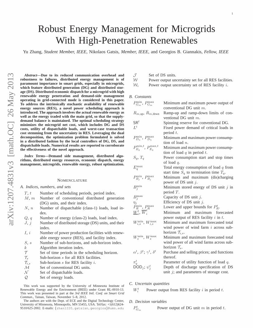
Microgrids operate in grid-connected or island mode, andmay entail distribution networks with residential or commer-cial end-users, in rural or urban areas. A typical configurationis depicted in Fig. 1; see also [1]. The microgrid energymanager (MGEM) coordinates the DERs and the controllableloads. Each of the DERs and loads has a local controller (LC),which coordinates with the MGEM the scheduling of resourcesthrough the communications infrastructure in a distributedfashion. The main challenge in energy scheduling is to accountfor the random and nondispatchable nature of the RES.

Optimal energy management for microgrids including eco-nomic dispatch (ED), unit commitment (UC), and demand-side management (DSM) is addressed in [2], but withoutpursuing a robust formulation against RES uncertainty. Based

House

LC

Fuel Gen.

MGEM

Grid

PHEV

LC

Elastic

Loads

Inelastic

Loads

Smart

Appliances

Hospital

Solar Wind

LC

Energy

Storage

LC

Fig. 1. Distributed control and computation architecture of a microgrid.

on the Weibull distribution for wind speed and the wind-speed-to-power-output mappings, an ED problem is formulated tominimize the risk of overestimation and underestimation ofavailable wind power [3]. Stochastic programming is also usedto cope with the variability of RES. Single-period chance-constrained ED problems for RES have been studied in [4],yielding probabilistic guarantees that the load will be served.Considering the uncertainties of demand profiles and PVgeneration, a stochastic program is formulated to minimizetheoverall cost of electricity and natural gas for a building in[5].Without DSM, robust scheduling problems with penalty-basedcosts for uncertain supply and demand have been investigatedin [6]. Recent works explore energy scheduling with DSM andRES using only centralized algorithms [7], [8]. An energysource control and DS planning problem for a microgrid isformulated and solved using model predictive control in [9].Distributed algorithms are developed in [10], but they onlyco-ordinate DERs to supply a given load without considering thestochastic nature of RES. Recently, a worst-case transactioncost based energy scheduling scheme has been proposed to ad-dress the variability of RESs through robust optimization thatcan also afford distributed implementation [11]. However,[11]considers only a single wind farm and no DS, and its approachcannot be readily extended to include multiple RESs and DS.

The present paper deals with optimal energy managementfor both supply and demand of a grid-connected microgridincorporating RES. The objective of minimizing the microgridnet cost accounts for conventional DG cost, utility of elasticloads, penalized cost of DS, and a worst-case transaction cost.The latter stems from the ability of the microgrid to sellexcess energy to the main grid, or to import energy in caseof shortage. Arobust formulation accounting for the worst-case amount of harvested RES is developed. A novel modelis introduced in order to maintain the supply-demand balancearising from the intermittent RES. Moreover, a transaction-price-based condition is established to ensure convexity ofthe overall problem (Section II). The separable structureand strong duality of the resultant problem are leveraged todevelop a low-overheaddistributed algorithm based on dualdecomposition, which is computationally efficient and resilientto communication outages or attacks. For faster convergence,the proximal bundle method is employed for the non-smoothsubproblem handled by the LC of RES (Section III). Nu-merical results corroborate the merits of the novel designs(Section IV), and the paper is wrapped up with a concluding

3

summary (Section V).Compared to [11], the contribution of the paper is threefold,

and of critical importance for microgrids with high-penetrationrenewables. First, a detailed model for DS is included, anddifferent design choices for storage cost functions are given toaccommodate, for example, depth-of-discharge specifications.Second, with the envisioned tide of high-penetration renewableenergy, multiple wind farms are considered alongside twopertinent uncertainty models. Finally, a new class of control-lable loads is added, with each load having a requirement oftotal energy over the scheduling horizon, as is the case withcharging of plug-in hybrid electric vehicles (PHEVs). Detailednumerical tests are presented to illustrate the merits of thescheduling decisions for the DG, DS, and controllable loads.Notation. Boldface lower case letters represent vectors;R

n

and R stand for spaces ofn × 1 vectors and real numbers,respectively;Rn

+ is the n-dimensional non-negative orthant;x′ transpose, and‖x‖ the Euclidean norm ofx.

II. ROBUST ENERGY MANAGEMENT FORMULATION

Consider a microgrid comprisingM conventional (fossilfuel) generators,I RES facilities, andJ DS units (see alsoFig. 1). The scheduling horizon isT := {1, 2, . . . , T } (e.g.,one-day ahead). The particulars of the optimal schedulingproblem are explained in the next subsections.

A. Load Demand Model

Loads are classified in two categories. The first comprisesinelastic loads, whose power demand should be satisfied atall times. Examples are power requirements of hospitals orillumination demand from residential areas.

The second category consists of elastic loads, which aredispatchable, in the sense that their power consumption isadjustable, and can be scheduled. These loads can be furtherdivided in two classes, each having the following characteris-tics:

i) The first class contains loads with power consumptionP tDn

∈ [PminDn

, PmaxDn

], where n ∈ N := {1, . . . , N},and t ∈ T . Higher power consumption yields higherutility for the end user. The utility function of thenthdispatchable load,U t

Dn(P t

Dn), is selected to be increasing

and concave, with typical choices being piecewise linearor smooth quadratic; see also [12]. An example from thisclass is an A/C.

ii) The second class includes loads indexed byq ∈ Q :={1, . . . , Q} with power consumption limitsPmin

Eqand

PmaxEq

, and prescribed total energy requirementsEq whichhave to be achieved from the start timeSq to termi-nation timeTq; see e.g., [13]. This type of loads canbe the plug-in hybrid electric vehicles (PHEVs). Powerdemand variables{P t

Eq}Tt=1 therefore are constrained as

∑Tq

t=SqP tEq

= Eq andP tEq

∈ [Pmin,tEq

, Pmax,tEq

], t ∈ T ,

while Pmin,tEq

= Pmax,tEq

= 0 for t /∈ {Sq, . . . , Tq}.Higher power consumption in earlier slots as opposedto later slots may be desirable for a certain load, sothat the associated task finishes earlier. This behavior

can be encouraged by adopting for theqth load anappropriately designed time-varying concave utility func-tion U t

Eq(P t

Eq). An example isU t

Eq(P t

Eq) := πt

qPtEq

,with weights{πt

q} decreasing int from slotsSq to Tq.Naturally,U t

Eq(P t

Eq) ≡ 0 can be selected if the consumer

is indifferent to how power is consumed across slots.

B. Distributed Storage Model

Let Btj denote the stored energy of thejth battery at the

end of the slott, with initial available energyB0j while Bmax

j

denotes the battery capacity, so that0 ≤ Btj ≤ Bmax

j , j ∈J := {1, . . . , J}. Let P t

Bjbe the power delivered to (drawn

from) the jth storage device at slott, which amounts tocharging (P t

Bj≥ 0) or discharging (P t

Bj≤ 0) of the battery.

Clearly, the stored energy obeys the dynamic equation

Btj = Bt−1

j + P tBj, j ∈ J , t ∈ T . (1)

VariablesP tBj

are constrained in the following ways:

i) The amount of (dis)charging is bounded, that is

PminBj

≤P tBj

≤ PmaxBj

(2)

−ηjBt−1

j ≤P tBj

(3)

with boundsPminBj

< 0 andPmaxBj

> 0, while ηj ∈ (0, 1]is the efficiency of DS unitj [14], [15]. The constraintin (3) means that a fractionηj of the stored energyBt−1

j

is available for discharge.ii) Final stored energy is also bounded for the sake of future

scheduling horizons, that isBTj ≥ Bmin

j .

To maximize DS lifetime, a storage costHtj(B

tj) can be

employed to encourage the stored energy to remain above aspecified depth of discharge, denoted asDODj ∈ [0, 1], where100% (0%) depth of discharge means the battery is empty(full) [15]. Such a cost is defined asHt

j(Btj) := ψt

j [(1 −DODj)B

maxj − Bt

j ]. Note that the storage costHtj(B

tj) can

be interpreted as imposing a soft constraint preventing largevariations of the stored energy. Clearly, higher weights{ψt

j}encourage smaller variation. If high power exchange is to beallowed, these weights can be chosen very small, or one caneven selectHt

j(Btj) ≡ 0 altogether.

C. Worst-case Transaction Cost

LetW ti denote theactualrenewable energy harvested by the

ith RES facility at time slott, and also letw collect allW ti ,

i.e., w := [W 11 , . . . ,W

T1 , . . . ,W

1I , . . . ,W

TI ]. To capture the

intrinsically stochastic and time-varying availability of RES,it is postulated thatw is unknown, but lies in a polyhedraluncertainty setW . The following are two practical examples.

i) The first example postulates a separate uncertainty setWi

for each RES facility in the form

Wi :=

{

{W ti }

Tt=1|W

ti ≤W t

i ≤Wt

i,

Wmini,s ≤

∑

t∈Ti,s

W ti ≤Wmax

i,s , T =

S⋃

s=1

Ti,s

}

(4)

4

whereW ti (W

t

i) denotes a lower (upper) bound onW ti ; T

is partitioned into consecutive but non-overlapping sub-horizonsTi,s for i = 1, . . . , I, s = 1, 2, . . . , S; the totalrenewable energy for theith RES facility over thesthsub-horizon is assumed bounded byWmin

i,s andWmaxi,s .

In this example,W takes the form of Cartesian product

W = W1 × . . .×WI . (5)

ii) The second example assumes a joint uncertainty modelacross all the RES facilities as

W :=

{

w|W ti ≤W t

i ≤Wt

i,

Wmins ≤

∑

t∈Ts

I∑

i=1

W ti ≤Wmax

s , T =

S⋃

s=1

Ts

}

(6)

whereW ti (W

t

i) denotes a lower (upper) bound onW ti ;

T is partitioned into consecutive but non-overlappingsub-horizonsTs for s = 1, 2, . . . , S; the total renewableenergy harvested by all the RES facilities over thesthsub-horizon is bounded byWmin

s andWmaxs ; see also [8].

The previous two RES uncertainty models are quite gen-eral and can take into account different geographical andmeteorological factors. The only information required is thedeterministic lower and upper bounds, namelyW t

i,Wt

i,Wmini,s ,

Wmaxi,s , Wmin

s , Wmaxs , which can be determined via inference

schemes based on historical data [16].Supposing the microgrid operates in a grid-connected mode,

a transaction mechanism between the microgrid and the maingrid is present, whereby the microgrid can buy/sell energyfrom/to the spot market. LetP t

R be an auxiliary variabledenoting the net power delivered to the microgrid from therenewable energy sources and the distributed storage in orderto maintain the supply-demand balance at slott. The shortage

energy per slott is given by[

P tR −

∑Ii=1

W ti +

∑Jj=1

P tBj

]+

,

while the surplus energy is[

P tR −

∑Ii=1

W ti +

∑Jj=1

P tBj

]−

,

where[a]+ := max{a, 0}, and [a]− := max{−a, 0}.The amount of shortage energy is bought with known

purchase priceαt, while the surplus energy is sold to themain grid with known selling priceβt. The worst-case nettransaction cost is thus given by

G({P tR}, {P

tBj

}) := maxw∈W

T∑

t=1

(

αt

[

P tR −

I∑

i=1

W ti +

J∑

j=1

P tBj

]+

− βt

[

P tR −

I∑

i=1

W ti +

J∑

j=1

P tBj

]−)

(7)

where {P tR} collects P t

R for t = 1, 2, . . . , T and {P tBj

}collectsP t

Bjfor j = 1, 2, . . . , J, t = 1, 2, . . . , T .

Remark 1. (Worst-case model versus stochastic model). Theworst-case robust model advocated here is particularly attrac-tive when the probability distribution of the renewable powerproduction is unavailable. This is for instance the case formul-tiple wind farms, where the spatio-temporal joint distribution

of the wind power generation is intractable (see detailed dis-cussions in [17] and [18]). If an accurate probabilistic modelis available, an expectation-based stochastic program canbeformulated to bypass the conservatism of worst-case optimiza-tion. In the case of wind generation, suppose that wind powerW t

i is a function of the random wind velocityvti , for whichdifferent models are available, and the wind-speed-to-power-output mappingsW t

i (vti) are known [19]. Then, the worst-case

transaction cost can be replaced by theexpectedtransactioncostG({P t

R}, {PtBj

}) := Ev

(

∑T

t=1αt[P t

R−∑I

i=1W t

i (vti)+

∑Jj=1

P tBj

]+−βt[P tR−

∑Ii=1

W ti (v

ti)+

∑Jj=1

P tBj

]−)

, where

v collectsvti for all i and t.

D. Microgrid Energy Management Problem

Apart from RES, microgrids typically entail also conven-tional DG. Let P t

Gmbe the power produced by themth

conventional generator, wherem ∈ M := {1, . . . ,M} andt ∈ T . The cost of themth generator is given by an increasingconvex functionCt

m(P tGm

), which typically is either piecewiselinear or smooth quadratic.

The energy management problem amounts to minimizingthe microgrid social net cost; that is, the cost of conventionalgeneration, storage, and the worst-case transaction cost (due tothe volatility of RES) minus the utility of dispatchable loads:

(P1) min{P t

Gm,P t

Dn,

P tEq

,Btj ,P

tBj

,P tR}

T∑

t=1

(

M∑

m=1

Ctm(P t

Gm)−

N∑

n=1

U tDn

(P tDn

)

−

Q∑

q=1

U tEq

(P tEq

) +

J∑

j=1

Htj(B

tj)

)

+G({P tR}, {P

tBj

}) (8a)

subject to:

PminGm

≤ P tGm

≤ PmaxGm

, m ∈ M, t ∈ T (8b)

P tGm

− P t−1

Gm≤ Rm,up, m ∈ M, t ∈ T (8c)

P t−1

Gm− P t

Gm≤ Rm,down, m ∈ M, t ∈ T (8d)

M∑

m=1

(PmaxGm

− P tGm

) ≥ SRt, t ∈ T (8e)

PminDn

≤ P tDn

≤ PmaxDn

, n ∈ N , t ∈ T (8f)

Pmin,tEq

≤ P tEq

≤ Pmax,tEq

, q ∈ Q, t ∈ T (8g)Tq∑

t=Sq

P tEq

= Eq, q ∈ Q (8h)

0 ≤ Btj ≤ Bmax

j , BTj ≥ Bmin

j , j ∈ J , t ∈ T (8i)

PminBj

≤ P tBj

≤ PmaxBj

, j ∈ J , t ∈ T (8j)

− ηjBt−1

j ≤ P tBj, j ∈ J , t ∈ T (8k)

Btj = Bt−1

j + P tBj, j ∈ J , t ∈ T (8l)

PminR ≤ P t

R ≤ PmaxR , t ∈ T (8m)

M∑

m=1

P tGm

+ P tR = Lt +

N∑

n=1

P tDn

+

Q∑

q=1

P tEq, t ∈ T . (8n)

Constraints (8b)–(8e) stand for the minimum/maximumpower output, ramping up/down limits, and spinning reserves,

5

respectively, which capture the typical physical requirementsof a power generation system. Constraints (8f) and (8m)correspond to the minimum/maximum power of the flexibleload demand and committed renewable energy. Constraint (8n)is the power supply-demandbalance equationensuring thetotal demand is satisfied by the power generation at any time.

Note that constraints (8b)–(8n) are linear, whileCtm(·),

−U tDn

(·), −U tEq

(·), and Htj(·) are convex (possibly non-

differentiable or non-strictly convex) functions. Consequently,the convexity of (P1) depends on that ofG({P t

R}, {PtBj

}),which is established in the following proposition.

Proposition 1. If the selling priceβt does not exceed the pur-chase priceαt for any t ∈ T , then the worst-case transactioncostG({P t

R}, {PtBj

}) is convex in{P tR} and {P t

Bj}.

Proof: Using that[a]++[a]− = |a|, and[a]+− [a]− = a,G({P t

R}, {PtBj

}) can be re-written as

G({P tR}, {P

tBj

}) = maxw∈W

T∑

t=1

(

δt

∣

∣

∣

∣

∣

P tR −

I∑

i=1

W ti +

J∑

j=1

P tBj

∣

∣

∣

∣

∣

+ γt

(

P tR −

I∑

i=1

W ti +

J∑

j=1

P tBj

))

(9)

with δt := (αt − βt)/2, and γt := (αt + βt)/2. Sincethe absolute value function is convex, and the operationsof nonnegative weighted summation and pointwise maximum(over an infinite set) preserve convexity [20, Sec. 3.2], theclaim follows readily.

An immediate corollary of Proposition 1 is that the energymanagement problem (P1) is convex ifβt ≤ αt for all t.The next section focuses on this case, and designs an efficientdecentralized solver for (P1).

III. D ISTRIBUTED ALGORITHM

In order to facilitate a distributed algorithm for (P1), a vari-able transformation is useful. Specifically, upon introducingP tR := P t

R +∑J

j=1P tBj

, (P1) can be re-written as

(P2) minx

T∑

t=1

(

M∑

m=1

Ctm(P t

Gm)−

N∑

n=1

U tDn

(P tDn

)

−

Q∑

q=1

U tEq

(P tEq

) +J∑

j=1

Htj(B

tj)

)

+G({P tR}) (10a)

subject to: (8b)− (8n)

P tR = P t

R +

J∑

j=1

P tBj, t ∈ T (10b)

where x collects all the primal variables{P t

Gm, P t

Dn, P t

Eq, P t

Bj, Bt

j , PtR, P

tR}; {P t

R} collects P tR

for t = 1, . . . , T ; and

G({P tR}) := max

w∈W

T∑

t=1

(

δt

∣

∣

∣

∣

∣

PtR −

I∑

i=1

Wti

∣

∣

∣

∣

∣

+ γt

(

PtR −

I∑

i=1

Wti

))

.

(11)

The following proposition extends the result of Proposition 1to the transformed problem, and asserts its strong duality.

Proposition 2. If (P2) is feasible, and the selling priceβt

does not exceed the purchase priceαt for any t ∈ T , thenthere is no duality gap.

Proof: Due to the strong duality theorem for the optimiza-tion problems with linear constraints (cf. [21, Prop. 5.2.1]),it suffices to show that the cost function is convex over theentire space and its optimal value is finite. First, using thesame argument, convexity ofG({P t

R}) in {P tR} is immediate

under the transaction price condition. The finiteness of theoptimal value is guaranteed by the fact that the continuousconvex cost (10a) is minimized over a nonempty compact setspecified by (8b)–(8n), and (10b).

The strong duality asserted by Proposition 2 motivates theuse of Lagrangian relaxation techniques in order to solve thescheduling problem. Moreover, problem (P2) is clearly sepa-rable, meaning that its cost and constraints are sums of terms,with each term dependent on different optimization variables.The features of strong duality and separability imply thatLagrangian relaxation and dual decomposition are applicableto yield a decentralized algorithm; see also related techniquesin power systems [22] and communication networks [23], [24].Coordinated by dual variables, the dual approach decomposesthe original problem into several separate subproblems thatcan be solved by the LCs in parallel. The development of thedistributed algorithm is undertaken next.

A. Dual Decomposition

Constraints (8e), (8n), and (10b) couple variables acrossgenerators, loads, and the RES. Letz collect dual variables{µt}, {λt}, and {νt}, which denote the corresponding La-grange multipliers. Keeping the remaining constraints implicit,the partial Lagrangian is given by

L(x, z) =T∑

t=1

(

M∑

m=1

Ctm(P t

Gm)−

N∑

n=1

U tDn

(P tDn

)

−

Q∑

q=1

U tEq

(P tEq

) +

J∑

j=1

Htj(B

tj)

)

+G({P tR})

+T∑

t=1

{

µt

(

SRt −

M∑

m=1

(PmaxGm

− P tGm

)

)

− λt

(

M∑

m=1

P tGm

+ P tR −

N∑

n=1

P tDn

−

Q∑

q=1

P tEq

− Lt

)

− νt

(

P tR − P t

R −J∑

j=1

P tBj

)}

. (12)

Then, the dual function can be written as

D(z) =minx

L(x, z)

s.t. (8b)− (8d), (8f) − (8m)

and the dual problem is given by

max D({µt}, {λt}, {νt}) (13a)

s.t. µt ≥ 0, λt, νt ∈ R, t ∈ T . (13b)

6

The subgradient method will be employed to obtain theoptimal multipliers and power schedules. The iterative processis described next, followed by its distributed implementation.

1) Subgradient Iterations: The subgradient methodamounts to running the recursions [25, Sec. 6.3]

µt(k + 1) = [µt(k) + agµt(k)]+ (14a)

λt(k + 1) = λt(k) + agλt(k) (14b)

νt(k + 1) = νt(k) + agνt(k) (14c)

wherek is the iteration index;a > 0 is a constant stepsize;while gµt(k), gλt(k), and gνt(k) denote the subgradients ofthe dual function with respect toµt(k), λt(k), and νt(k),respectively. These subgradients can be expressed in the fol-lowing simple forms

gµt(k) = SRt −

M∑

m=1

(PmaxGm

− P tGm

(k)) (15a)

gλt(k) = Lt +

N∑

n=1

P tDn

(k) +

Q∑

q=1

P tEq

(k)

−M∑

m=1

P tGm

(k)− P tR(k) (15b)

gνt(k) = P tR(k) +

J∑

j=1

P tBj

(k)− P tR(k) (15c)

whereP tGm

(k), P tDn

(k), P tEq

(k), P tBj

(k), P tR(k), andP t

R(k)are given by (16)–(20).

Iterations are initialized with arbitraryλt(0), νt(0) ∈ R,andµt(0) ≥ 0. The iterates are guaranteed to converge to aneighborhood of the optimal multipliers [25, Sec. 6.3]. Thesize of the neighborhood is proportional to the stepsize, andcan therefore be controlled by the stepsize.

When the primal objective isnot strictly convex, a primalaveraging procedure is necessary to obtain the optimal power

schedules, which are then given by

x(k) =1

k

k−1∑

j=0

x(j) =1

kx(k − 1) +

k − 1

kx(k − 1). (21)

The running averages can be recursively computed as in (21),and are also guaranteed to converge to a neighborhood of theoptimal solution [26]. Note that other convergence-guaranteedstepsize rules and primal averaging methods can also beutilized; see [27] for detailed discussions.

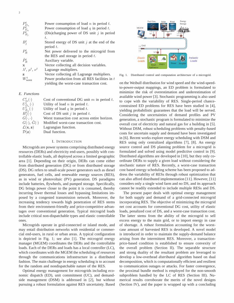
2) Distributed Implementation:The form of the subgradi-ent iterations easily lends itself to a distributed implementationutilizing the control and communication capabilities of atypical microgrid.

Specifically, the MGEM maintains and updates the La-grange multipliers via (14). The LCs of conventional gen-eration, dispatchable loads, storage units, and RES solvesubproblems (16)–(20), respectively. These subproblems canbe solved if the MGEM sends the current multiplier iteratesµt(k), λt(k), and νt(k) to the LCs. The LCs send backto the MGEM the quantities

∑M

m=1P tGm

(k),∑N

n=1P tDn

(k),∑Q

q=1P tEq

(k),∑J

j=1P tBj

(k), P tR(k), and P t

R(k) which arein turn used to form the subgradients according to (15). Thedistributed algorithm using dual decomposition is tabulated asAlgorithm 1, and the interactive process of message passingis illustrated in Fig. 2.

MGEM

LC of

RES

LC of

DS

j

t

BjPå

,t tn l

,t t

R RP Pt t

R RP Pt tt t

R R

LC of

2ndClass

Loadstl

LC of

1stClass

Loads

n

t

DnPå

q

t

EqPå

LC of

Fuel

Gen.

m

t

GmPå ,

t tl m

Fig. 2. Decomposition and message exchange.

{P tGm

(k)}Tt=1 ∈ argmin{P t

Gm}

s.t. (8b)−(8d)

{

T∑

t=1

(

Ctm(P t

Gm) +

(

µt(k)− λt(k))

P tGm

)

}

(16)

{P tDn

(k)}Tt=1 ∈ argmin{P t

Dn}

s.t. (8f)

{

T∑

t=1

(

λt(k)P tDn

− U tDn

(P tDn

)

)

}

(17)

{P tEq

(k)}Tt=1 ∈ argmin{P t

Eq}

s.t. (8g)−(8h)

{

T∑

t=1

(

λt(k)P tEq

− U tEq

(P tEq

)

)

}

(18)

{P tBj

(k)}Tt=1 ∈ argmin{P t

Bj,Bt

j}

s.t. (8i)−(8l)

{

T∑

t=1

(

νt(k)P tBj

+Htj(B

tj)

)

}

(19)

{P tR(k), P

tR(k)}

Tt=1 ∈ argmin

{P tR,P t

R}s.t. (8m)

{

T∑

t=1

(

(

νt(k)− λt(k))

P tR

)

+G({P tR})−

T∑

t=1

νt(k)P tR

}

(20)

7

Algorithm 1 Distributed Energy Management

1: Initialize Lagrange multipliersλt = µt = νt = 02: repeat (k = 0, 1, 2, . . .)3: for t = 1, 2, . . . , T do4: Broadcastλt(k), µt(k), andνt(k) to LCs of con-

vectional generators, controllable loads, storage units,andRES facilities

5: Update power schedulingP tGm

(k), P tDn

(k),P tEq

(k), P tBj

(k), P tR(k), andP t

R(k) by solving (16)–(20)6: Updateλt(k), µt(k), andνt(k) via (14)7: end for8: Running averages of primal variables via (21)9: until Convergence

Algorithm 2 Enumerate all the vertices of a polytopeA

1: Initialize vertex setV = ∅2: Generate setA := {a ∈ R

n|ai = ai or ai, i = 1, . . . , n};check the feasibility of all the points in setA, i.e., ifamin ≤ 1′a ≤ amax}, thenV = V ∪ {a}

3: Generate setA := {a ∈ Rn|ai = amin −

∑

j 6=i aj or amax −∑

j 6=i aj , aj = aj or aj , i, j =1, . . . , n, j 6= i}; check the feasibility of all the pointsin set A, i.e., if a � a � a, thenV = V ∪ {a}

B. Solving the LC Subproblems

This subsection shows how to solve each subproblem (16)–(20). Specifically,Ct

m(·), −U tDn

(·), −U tEq

(·), andHtj(·) are

chosen either convex piece-wise linear or smooth convexquadratic. Correspondingly, the first four subproblems (16)–(19) are essentially linear programs (LPs) or quadratic pro-grams (QPs), which can be solved efficiently. Therefore, themain focus is on solving (20).

The optimal solution ofP tR(k) in (20) is easy to obtain as

P tR(k) =

{

PminR , if νt(k) ≥ λt(k)

PmaxR , if νt(k) < λt(k).

(22)

However, due to the absolute value operator and the maximiza-tion overw in the definition ofG({P t

R}), subproblem (20)is a convex nondifferentiable problem in{P t

R}, which canbe challenging to solve. As a state-of-the-art technique forconvex nondifferentiable optimization problems [25, Ch. 6],the bundle method is employed to obtain{P t

R(k)}.Upon defining

G({P tR}) := G({P t

R})−T∑

t=1

νt(k)P tR (23)

the subgradient ofG({P tR}) with respect toP t

R needed forthe bundle method can be obtained by the generalization ofDanskin’s Theorem [25, Sec. 6.3] as

∂G({P tR}) =

αt − νt(k), if P tR ≥

I∑

i=1

(W ti )

∗

βt − νt(k), if P tR <

I∑

i=1

(W ti )

∗

(24)

Algorithm 3 Enumerate all the vertices of a polytopeB1: for i = 1, 2, . . . , S do2: Obtain vertex setVs by applying Algorithm 2 toBs

3: end for4: Generate verticesbv for B by concatenating all the indi-

vidual verticesbs asbv = [(bv1)

′, . . . , (bvS)

′]′, bs ∈ Vs

where for given{P tR} it holds that

w∗ ∈ argmax

w∈W

{

T∑

t=1

(

δt

∣

∣

∣

∣

∣

PtR −

I∑

i=1

Wti

∣

∣

∣

∣

∣

+ γt

(

PtR −

I∑

i=1

Wti

))}

.

(25)

With p := [P 1R, . . . , P

TR ], the bundle method generates a

sequence{pℓ} with guaranteed convergence to the optimal{P t

R(k)}; see e.g., [28], [25, Ch. 6]. The iteratepℓ+1 isobtained by minimizing a polyhedral approximation ofG(p)with a quadratic proximal regularization as follows

pℓ+1 := argminp∈RT

{

Gℓ(p) +ρℓ2‖p− yℓ‖

2

}

(26)

where Gℓ(p) := max{G(p0) + g′0(p − p0), . . . , G(pℓ) +

g′ℓ(p − pℓ)}; gℓ is the subgradient ofG(p) evaluated at the

pointp = pℓ, which is calculated according to (24); proximityweightρℓ is to control stability of the iterates; and the proximalcenteryℓ is updated according to a query for descent

yℓ+1 =

{

pℓ+1, if G(yℓ)− G(pℓ+1) ≥ θηℓyℓ, otherwise

(27)

where ηℓ = G(yℓ) −(

Gℓ(pℓ+1) +ρℓ

2‖pℓ+1 − yℓ‖2

)

, θ ∈

(0, 1).It is worth mentioning that (26) is essentially a QP over

a simplex in the dual space, which is efficiently solvable bypractical optimization algorithms. The corresponding transfor-mation is shown in Appendix I for the interested readers.

Algorithms for solving (25) depend on the form of theuncertainty setW , and are elaborated next.

C. Vertex Enumerating Algorithms

In order to obtainw∗, the convex nondifferentiable functionin (25) should be maximized overW . This is generally an NP-hard convex maximization problem. However, for the specificproblem here, the special structure of the problem can beutilized to obtain a computationally efficient approach.

Specifically, the global solution is attained at the extremepoints of the polytope [25, Sec. 2.4]. Therefore, the objectivein (25) can be evaluated at all vertices ofW to obtainthe global solution. Since there are only finitely many ver-tices, (25) can be solved in afinite number of steps.

For the polytopesW with special structure [cf. (4), (6)],characterizations of vertices are established in Propositions 3and 4. Capitalizing on these propositions, vertex enumeratingprocedures are designed consequently, and are tabulated asAlgorithms 2 and 3.

Proposition 3. For a polytopeA := {a ∈ Rn|a � a �

a, amin ≤ 1′a ≤ amax}, av ∈ A is a vertex (extreme point)

8

TABLE IGENERATING CAPACITIES, RAMPING LIMITS , AND COST COEFFICIENTS.THE UNITS OFam AND bm ARE $/(KWH)2 AND $/KWH, RESPECTIVELY.

Unit Pmin

GmPmax

GmRm,up(down) am bm

1 10 50 30 0.006 0.52 8 45 25 0.003 0.253 15 70 40 0.004 0.3

TABLE IICLASS-1 DISPATCHABLE LOADS PARAMETERS. THE UNITS OFcn AND dn

ARE $/(KWH)2 AND $/KWH, RESPECTIVELY.

Load 1 Load 2 Load 3 Load 4 Load 5 Load 6

Pmin

Dn0.5 4 2 5.5 1 7

Pmax

Dn10 16 15 20 27 32

cn -0.002 -0.0017 -0.003 -0.0024 -0.0015 -0.0037dn 0.2 0.17 0.3 0.24 0.15 0.37

of A if and only if it has one of the following forms: i)avi =

ai or ai for i = 1, . . . , n; or ii) avi = amin−

∑

j 6=i avj or amax−

∑

j 6=i avj , a

vj = aj or aj , for i, j = 1, . . . , n, j 6= i.

Proof: See Appendix II-A.Essentially, Proposition 3 verifies the geometric character-

ization of vertices. SinceW is the part of a hyperrectangle(orthotope) between two parallel hyperplanes, its vertices canonly either be the hyperrectangle’s vertices which are not cutaway, or, the vertices of the intersections of the hyperrectangleand the hyperplanes, which must appear in some edges of thehyperrectangle.

Next, the vertex characterization of a polytope in a Cartesianproduct formed by many lower-dimensional polytopes likeAis established, which is needed for the uncertainty set (4).

Proposition 4. Assumeb ∈ Rn is divided intoS consecutive

and non-overlapping blocks asb = [b′1, . . . ,b

′S ]

′, wherebs ∈R

ns and∑S

s=1ns = n. Consider a polytopeB := {b ∈

Rn|b � b � b, bmin

s ≤ 1′nsbs ≤ bmax

s , s = 1, . . . , S}. Thenbv = [(bv

1)′, . . . , (bv

S)′]′ is a vertex ofB if and only if for

s = 1, . . . , S, bvs is the vertex of a lower-dimensional polytope

Bs := {bs ∈ Rns |bs � bs � bs, b

mins ≤ 1′

nsbs ≤ bmax

s }.

Proof: See Appendix II-B.Algorithms 2 and 3 can be used to to generate the vertices

of uncertainty sets (4) and (6) as described next.

i) For uncertainty set (4), first use Algorithm 2 to obtainthe vertices corresponding to each sub-horizonTi,s forall the RES facilities. Then, concatenate the obtainedvertices to get the ones for each RES facility by Step 4in Algorithm 3. Finally, run this step again to form thevertices of (4) by concatenating the vertices of eachWi.

ii) For uncertainty sets (6), use Algorithm 2 to obtain thevertices for each sub-horizonTs. Note that concatenatingstep in Algorithm 3 is not needed in this case becauseproblem (25) is decomposable across sub-horizonsTs,s = 1, . . . , S, and can be independently solved accord-ingly.

After the detailed description of vertex enumerating proce-dures for RES uncertainty sets, a discussion on the complexityof solving (25) follows.

TABLE IIICLASS-2 DISPATCHABLE LOADS PARAMETERS

Load 1 Load 2 Load 3 Load 4

Pmin

Eq0 0 0 0

Pmax

Eq1.2 1.55 1.3 1.7

Emaxq 5 5.5 4 8Sq 6PM 7PM 6PM 6PMTq 12AM 11PM 12AM 12AM

TABLE IVL IMITS OF FORECASTED WIND POWER

Slot 1 2 3 4 5 6 7 8

W t1

2.47 2.27 2.18 1.97 2.28 2.66 3.1 3.38

Wt1 24.7 22.7 21.8 19.7 22.8 26.6 31 33.8

W t2

2.57 1.88 2.16 1.56 1.95 3.07 3.44 3.11

Wt2 25.7 18.8 21.6 15.6 19.5 30.7 34.4 31.1

Remark 2. (Complexity of solving(25)). Vertex enumerationincurs exponential complexity because the number of verticescan increase exponentially with the number of variables andconstraints [29, Ch. 2]. However, if the cardinality of eachsub-horizonTs is not very large (e.g., when24 hours are parti-tioned into4 sub-horizons each comprising6 time slots), thenthe complexity is affordable. Most importantly, the vertices ofW need only be listed once, before optimization.

IV. N UMERICAL TESTS

In this section, numerical results are presented to verify theperformance of the robust and distributed energy scheduler.The Matlab-based modeling packageCVX [30] along withthe solverMOSEK [31] are used to specify and solve theproposed robust energy management problem. The consideredmicrogrid consists ofM = 3 conventional generators,N = 6class-1 dispatchable loads,Q = 4 class-2 dispatchable loads,J = 3 storage units, andI = 2 renewable energy facilities(wind farms). The time horizon spansT = 8 hours, corre-sponding to the interval4PM–12AM. The generation costsCm(PGm

) = amP2Gm

+ bmPGmand the utilities of class-

1 elastic loadsUn(PDn) = cnP

2Dn

+ dnPDnare set to be

quadratic and time-invariant. Generator parameters are given inTable I, whileSRt = 10kWh. The relevant parameters of twoclasses of dispatchable loads are listed in Tables II and III(seealso [27]). The utility of class-2 loads isU t

Eq(P t

Eq) := πt

qPtEq

with weightsπtq = 4, 3.5, . . . , 1, 0.5 for t = 4PM, . . . , 11PM

andq ∈ Q.Three batteries have capacityBmax

j = 30kWh (similarto [5]). The remaining parameters arePmin

Bj= −10kWh,

PmaxBj

= 10kWh, B0j = Bmin

j = 5kWh, andηj = 0.95, for allj ∈ J . The battery costsHt

j(Btj) are set to zero. The joint

uncertainty model withS = 1 is considered forW [cf. (6)],whereWmin

1 = 40kWh, andWmax1 = 360kWh. In order

to obtainW ti andW

t

i listed in Table IV, MISO day-aheadwind forecast data [32] are rescaled to the order of1 kWhto 40 kWh, which is a typical wind power generation for amicrogrid [33].

Similarly, the fixed loadLt in Table V is a rescaled versionof the cleared load provided by MISO’s daily report [34]. For

9

TABLE VFIXED LOADS DEMAND AND TRANSACTION PRICES. THE UNITS OFαt

AND βt ARE ¢/KWH.

Slot 1 2 3 4 5 6 7 8

Lt 57.8 58.4 64 65.1 61.5 58.8 55.5 51(Case A)αt 2.01 2.2 3.62 6.6 5.83 3.99 2.53 2.34βt 1.81 1.98 3.26 5.94 5.25 3.59 2.28 2.11(Case B)αt 40.2 44 72.4 132 116.6 79.8 50.6 46.8βt 36.18 39.6 65.16 118.8 104.94 71.82 45.54 42.12

4PM 5PM 6PM 7PM 8PM 9PM 10PM 11PM 12AM0

20

40

60

80

100

120

Time slot

Pow

er s

ched

ulin

g (k

Wh)

P t

G

P t

R

P t

D

P t

E

Lt

W tworst

Fig. 3. Optimal power schedules: Case A.

the transaction prices, two different cases are studied as givenin Table V, where{αt} in Case A are real-time prices of theMinnesota hub in MISO’s daily report. To evaluate the effectof high transaction prices,{αt} in Case B is set as20 timesof that in Case A. For both cases,βt = 0.9αt, which satisfiesthe convexity condition for (P1) given in Proposition 1.

The optimal microgrid power schedules of two cases areshown in Figs. 3 and 4. The stairstep curves includeP t

G :=∑

m P tGm

, P tD :=

∑

n PtDn

, and P tE :=

∑

q PtEq

denotingthe total conventional power generation, and total elasticdemand for classes 1 and 2, respectively, which are the optimalsolutions of (P2). QuantityW t

worst denotes the total worst-casewind energy at slott, which is the optimal solution of (25)with optimal P t

R.A common observation from Figs. 3 and 4 is that the total

conventional power generationP tG varies with the same trend

acrosst as the fixed load demandLt, while the class-1 elasticload exhibits the opposite trend. Because the conventionalgeneration and the power drawn from the main grid arelimited, the optimal scheduling by solving (P2) dispatcheslesspower forP t

D whenLt is large (from6PM to 10PM), and viceversa. This behavior indeed reflects the load shifting ability ofthe proposed design for the microgrid energy management.

Furthermore, by comparing two cases in Figs. 3 and 4, itis interesting to illustrate the effect of the transaction prices.Remember that the difference betweenP t

R and W tworst is

the shortage power needed to purchase (if positive) or thesurplus power to be sold (if negative), Figs. 3 shows thatthe microgrid always purchases energy from the main gridbecauseP t

R is more thanW tworst. This is because for Case

A, the purchase priceαt is much lower than the marginalcost of the conventional generation (cf. Tables I and V). The

4PM 5PM 6PM 7PM 8PM 9PM 10PM 11PM 12AM−20

0

20

40

60

80

100

120

Time slot

Pow

er s

ched

ulin

g (k

Wh)

P t

G

P t

R

P t

D

P t

E

Lt

W tworst

Fig. 4. Optimal power schedules: Case B.

Case A Case B

−50

0

50

100

150

200

250

Opt

imal

cos

ts (

$)

Conventional generation costNegative utility of class−1 loadsNegative utility of class−2 loadsWorst−case transaction costMicrogrid net cost

Fig. 5. Optimal costs: Case A and B.

economic scheduling decision is thus to reduce conventionalgeneration while purchasing more power to keep the supply-demand balance. For Case B, sinceαt is much higher than thatin Case A, less power should be purchased which is reflectedin the relatively small gap betweenP t

R andW tworst across time

slots. It can also be seen thatP tR is smaller thanW t

worst from7PM to 9PM, meaning that selling activity happens and isencouraged by the highest selling priceβt in these slots acrossthe entire time horizon. Moreover, selling activity results inthe peak conventional generation from7PM to 9PM. Fig. 5compares the optimal costs for the two cases. It can be seenthat the optimal costs of conventional generation and worst-case transaction of Case B are higher than those of Case A,which can be explained by the higher transaction prices andthe resultant larger DG output for Case B.

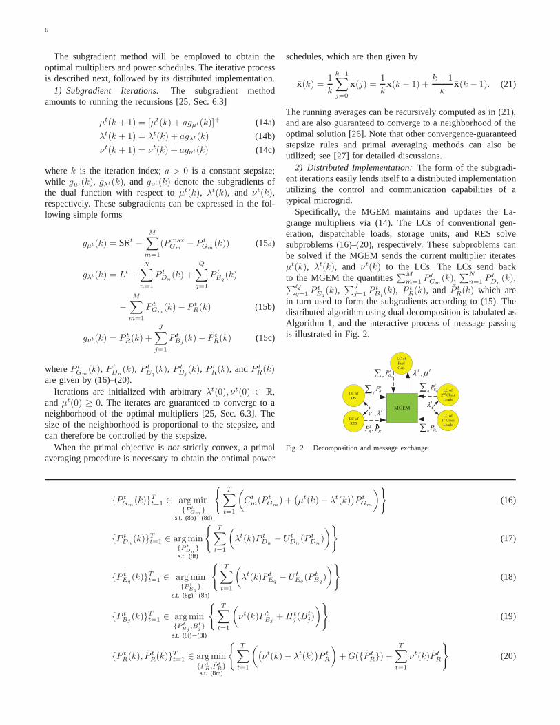
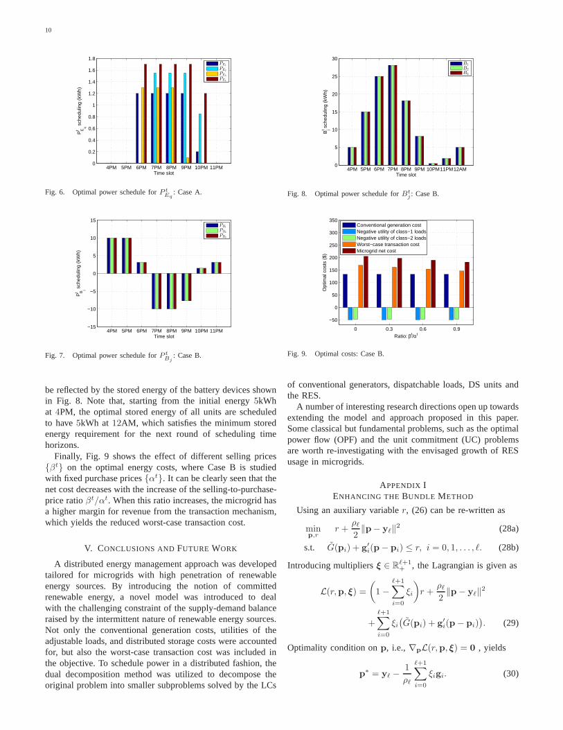
The optimal power scheduling of class-2 elastic load isdepicted in Fig. 6 for Case A. Due to the start timeSq

(cf. Table III), zero power is scheduled for the class-2 load1, 3, and 4 from4PM to 6PM while from 4PM to 7PM forthe load 2. The decreasing trend for all such loads is due to thedecreasing weights{πt

q} from Sq to Tq, which is establishedfrom the fast charging motivation for the PHEVs, for example.

Figs. 7 depicts the optimal charging or discharging powerof the DSs for Case B. Clearly, all DSs are discharging duringthe three slots of7PM, 8PM, and9PM. This results from themotivation of selling more or purchasing less power becauseboth purchase and selling prices are very high during theseslots (cf. Table V). The charging (discharging) activity can also

10

4PM 5PM 6PM 7PM 8PM 9PM 10PM 11PM0

0.2

0.4

0.6

0.8

1

1.2

1.4

1.6

1.8

Time slot

PE

q

t s

ched

ulin

g (k

Wh)

PE1

PE2

PE3

PE4

Fig. 6. Optimal power schedule forP tEq

: Case A.

4PM 5PM 6PM 7PM 8PM 9PM 10PM 11PM−15

−10

−5

0

5

10

15

Time slot

PB

j

t s

ched

ulin

g (k

Wh)

PB1

PB2

PB3

Fig. 7. Optimal power schedule forP tBj

: Case B.

be reflected by the stored energy of the battery devices shownin Fig. 8. Note that, starting from the initial energy5kWhat 4PM, the optimal stored energy of all units are scheduledto have5kWh at 12AM, which satisfies the minimum storedenergy requirement for the next round of scheduling timehorizons.

Finally, Fig. 9 shows the effect of different selling prices{βt} on the optimal energy costs, where Case B is studiedwith fixed purchase prices{αt}. It can be clearly seen that thenet cost decreases with the increase of the selling-to-purchase-price ratioβt/αt. When this ratio increases, the microgrid hasa higher margin for revenue from the transaction mechanism,which yields the reduced worst-case transaction cost.

V. CONCLUSIONS ANDFUTURE WORK

A distributed energy management approach was developedtailored for microgrids with high penetration of renewableenergy sources. By introducing the notion of committedrenewable energy, a novel model was introduced to dealwith the challenging constraint of the supply-demand balanceraised by the intermittent nature of renewable energy sources.Not only the conventional generation costs, utilities of theadjustable loads, and distributed storage costs were accountedfor, but also the worst-case transaction cost was included inthe objective. To schedule power in a distributed fashion, thedual decomposition method was utilized to decompose theoriginal problem into smaller subproblems solved by the LCs

4PM 5PM 6PM 7PM 8PM 9PM 10PM11PM12AM0

5

10

15

20

25

30

Time slot

Bjt s

ched

ulin

g (k

Wh)

B1

B2

B3

Fig. 8. Optimal power schedule forBtj : Case B.

0 0.3 0.6 0.9

−50

0

50

100

150

200

250

300

350

Ratio: βt/αt

Opt

imal

cos

ts (

$)

Conventional generation costNegative utility of class−1 loadsNegative utility of class−2 loadsWorst−case transaction costMicrogrid net cost

Fig. 9. Optimal costs: Case B.

of conventional generators, dispatchable loads, DS units andthe RES.

A number of interesting research directions open up towardsextending the model and approach proposed in this paper.Some classical but fundamental problems, such as the optimalpower flow (OPF) and the unit commitment (UC) problemsare worth re-investigating with the envisaged growth of RESusage in microgrids.

APPENDIX IENHANCING THE BUNDLE METHOD

Using an auxiliary variabler, (26) can be re-written as

minp,r

r +ρℓ2‖p− yℓ‖

2 (28a)

s.t. G(pi) + g′i(p− pi) ≤ r, i = 0, 1, . . . , ℓ. (28b)

Introducing multipliersξ ∈ Rℓ+1+ , the Lagrangian is given as

L(r,p, ξ) =

(

1−ℓ+1∑

i=0

ξi

)

r +ρℓ2‖p− yℓ‖

2

+

ℓ+1∑

i=0

ξi(

G(pi) + g′i(p− pi)

)

. (29)

Optimality condition onp, i.e.,∇pL(r,p, ξ) = 0 , yields

p∗ = yℓ −1

ρℓ

ℓ+1∑

i=0

ξigi. (30)

11

Substituting (30) into (29), the dual of (28) is

maxξ

−1

2ρℓ

∥

∥

∥

∥

∥

ℓ+1∑

i=0

ξigi

∥

∥

∥

∥

∥

2

+

ℓ+1∑

i=0

ξi(

G(pi) + g′i(yℓ − pi)

)

(31a)

s.t. ξ � 0, 1′ξ = 1 (31b)

where1 is the all-ones vector.Note that (31) is essentially a QP over the simplex inR

ℓ+1,which can be solved very efficiently.

APPENDIX IIPROOFS OFPROPOSITIONS

To prove Propositions 3 and 4, the following lemma isneeded, which shows sufficient and necessary conditions fora point to be a vertex of a polytope represented as a linearsystem [35, Sec. 3.5].

Lemma 1. For a polytopeP := {x ∈ Rn|Ax � c}, a point

v ∈ P is a vertex if and only if there exists a subsystemAx � c of Ax � c so that rank(A) = n andv is the unique(feasible) solution ofAv = c.

A. Proof of Proposition 3

The polytopeA := {a ∈ Rn|a � a � a, amin ≤ 1′a ≤

amax} can be re-written asA := {a ∈ Rn|Aa � c}, where

A := [In×n,−In×n,1,−1]′ andc := [a′,−a′, amax,−amin]′.By Lemma 1, enumerating vertices ofA is equivalent tofinding all feasible solutions of the linear subsystemsAa = c,such that rank-n matrix A is constructed by extracting rowsof A. It can be seen that such full column-rank matrixA canonly have two forms (with row permutation if necessary): i)A1 = diag(d) with di ∈ {−1, 1}, i = 1, . . . , n; ii) A2(i, :) =±1′, i = 1, . . . , n, andA2(j, :) = A1(j, :), ∀j 6= i. Basically,A1 is constructed by choosingn vectors as a basis ofRn fromthe first2n rows ofA. Substituting any row ofA1 with ±1′,forms A2. Finally, by solving all the linear subsystems of theform Aka = ck, for k = 1, 2, Proposition 3 follows readily.

B. Proof of Proposition 4

The polytopeB := {b ∈ Rn|b � b � b, bmin

s ≤ 1′nsbs ≤

bmaxs , s = 1, . . . , S} can be re-written asB := {b ∈ R

n|Bb �c}, whereB := diag(B1, . . . ,BS), c := [c′1, . . . , c

′S ]

′, Bs :=[Ins×ns

,−Ins×ns,1,−1]′, andcs := [a′s,−a′s, b

maxs ,−bmin

s ]′

for s = 1, . . . , S.Similarly by Lemma 1, all the vertices ofB can be enumer-

ated by solvingBb = c, where the rank-n matrix B is formedby extracting rows ofB. Due to the block diagonal structureof B, it can be seen that the only way to find itsn linearindependent rows is to findns linear independent vectors fromthe rows corresponding toBs for s = 1, . . . , S. In otherwords, the verticesbv can be obtained by concatenating allthe individual verticesbs as stated in Proposition 4.

REFERENCES

[1] N. Hatziargyriou, H. Asano, R. Iravani, and C. Marnay, “Microgrids:An overview of ongoing research, development, and demonstrationprojects,” IEEE Power & Energy Mag., vol. 5, no. 4, pp. 78–94, July–Aug. 2007.

[2] P. Stluka, D. Godbole, and T. Samad, “Energy management for buildingsand microgrids,” inProc. of the 50th IEEE Conf. on Decision andControl and European Control Conf., Orlando, FL, Dec. 12–15, 2011.

[3] J. Hetzer, C. Yu, and K. Bhattarai, “An economic dispatchmodelincorporating wind power,”IEEE Trans. on Energy Conver., vol. 23,no. 2, pp. 603–611, June 2008.

[4] X. Liu and W. Xu, “Economic load dispatch constrained by wind poweravailability: A here-and-now approach,”IEEE Trans. on SustainableEnergy, vol. 1, no. 1, pp. 2–9, Apr. 2010.

[5] X. Guan, Z. Xu, and Q.-S. Jia, “Energy-efficient buildings facilitatedby microgrid,” IEEE Trans. on Smart Grid, vol. 1, no. 3, pp. 243–252,Dec. 2010.

[6] D. Bertsimas, E. Litvinov, X. Sun, J. Zhao, and T. Zheng, “Adap-tive robust optimization for the security constrained unitcommitmentproblem,” Mar. 2011, [Online]. Available: http://web.mit.edu/sunx/www/Adaptive Robust UC Revision.pdf.

[7] L. Jiang and S. H. Low, “Real-time demand response with uncertainrenewable energy in smart grid,” inProc. of the 49th Allerton Conf.on Comm., Control, and Computing, Monticello, IL, Sept. 2011, pp.1334–1341.

[8] L. Zhao and B. Zeng, “Robust unit commitment problem withde-mand response and wind energy,” Univ. of S. Florida, Tech. Rep.,Oct. 2010, [Online]. Available: http://www.optimization-online.org/DBFILE/2010/11/2784.pdf.

[9] C. Jin and P. K. Ghosh, “Coordinated usage of distributedsources forenergy cost saving in micro-grid,” inProc. of the 43rd North AmericanPower Symposium (NAPS), Boston, MA, Aug. 4–6, 2011.

[10] A. D. Domınguez-Garcıa and C. N. Hadjicostis, “Distributed algorithmsfor control of demand response and distributed energy resources,” inProc. of the 50th IEEE Control and Decision Conf., Orlando, FL, Dec.2011.

[11] Y. Zhang, N. Gatsis, and G. B. Giannakis, “Robust distributed energymanagement for microgrids with renewables,” inProc. of 3rd Intl. Conf.on Smart Grid Commun., Tainan, Taiwan, Nov. 5–8, 2012.

[12] L. Chen, N. Li, S. H. Low, and J. C. Doyle, “Two market models fordemand response in power networks,” inProc. 1st IEEE Intl. Conf. SmartGrid Communications, Gaithersburg, MD, Oct. 2010, pp. 397–402.

[13] A.-H. Mohsenian-Rad, V. S. W. Wong, J. Jatskevich, R. Schober,and A. Leon-Garcia, “Autonomous demand side management basedon game-theoretic energy consumption scheduling for the future smartgrid,” IEEE Trans. on Smart Grid, vol. 1, no. 3, pp. 320–331, Dec. 2010.

[14] P. Vytelingum, T. D. Voice, S. D. Ramchurn, A. Rogers, and N. R.Jennings, “Agent-based micro-storage management for the smart grid,”in Proc. 9th Intl. Conf. Autonomous and Multiagent Systems, Toronto,Canada, May 2010, pp. 39–46.

[15] V. Alimisis and N. Hatziargyriou, “Evaluation of a hybrid power plantcomprising used EV-batteries to complement wind power,”IEEE Trans.on Sustainable Energy, vol. 4, no. 2, pp. 286–293, Apr. 2013.

[16] P. Pinson and G. Kariniotakis, “Conditional prediction intervals of windpower generation,”IEEE Trans. on Power Syst., vol. 25, no. 4, pp. 1845–1856, Nov. 2010.

[17] Y. Zhang, N. Gatsis, and G. B. Giannakis, “Risk-constrained energymanagement with multiple wind farms,” inProc. of 4th IEEE Conf.Innovative Smart Grid Tech., Washington, D.C., Feb. 24–27, 2013.

[18] J. M. Morales, L. Baringo, A. J. Conejo, and R. Mınguez,“Probabilisticpower flow with correlated wind sources,”IET Generation, Transmission& Distribution, vol. 4, no. 5, pp. 641–651, May 2010.

[19] J. A. Carta, P. Ramırez, and S. Velazquez, “A review ofwind speedprobability distributions used in wind energy analysis: Case studies inthe canary islands,”Renew. Sust. Energ. Rev., vol. 13, pp. 933–955,2009.

[20] S. Boyd and L. Vandenberghe,Convex Optimization. U.K.: CambridgeUniversity Press, 2004.

[21] D. P. Bertsekas,Nonlinear Programming, 2nd ed. Belmont, MA:Athena Scientific, 1999.

[22] A. J. Conejo, E. Castillo, R. Mınguez, and R. Garcıa-Bertrand,Decom-position Techniques in Mathematical Programming: Engineering andScience Applications. Springer, 2006.

[23] D. Palomar and M. Chiang, “A tutorial on decomposition methods fornetwork utility maximization,” IEEE J. Sel. Areas Commun., vol. 46,no. 8, pp. 1439–1451, Aug. 2006.

12

[24] M. Chiang, S. H. Low, A. R. Calderbank, and J. C. Doyle, “Layeringas optimization decomposition: A mathematical theory of networkarchitectures,”Proc. of the IEEE, vol. 95, no. 1, pp. 255–312, Jan. 2007.

[25] D. P. Bertsekas,Convex Optimization Theory. Belmont, MA: AthenaScientific, 2009.

[26] A. Nedic and A. Ozdaglar, “Approximate primal solutions and rateanalysis for dual subgradient methods,”SIAM J. Optim., vol. 19, no. 4,pp. 1757–1780, 2009.

[27] N. Gatsis and G. B. Giannakis, “Residential load control: Distributedscheduling and convergence with lost AMI messages,”IEEE Trans. onSmart Grid, vol. 3, no. 2, pp. 770–786, June 2012.

[28] S. Feltenmark and K. C. Kiwiel, “Dual application of proximal bundlemethods, including Lagrange relaxation of nonconvex problems,” SIAMJ. Optim., vol. 10, no. 3, pp. 697–721, Feb./Mar. 2000.

[29] D. Bertsimas and J. N. Tsitsiklis,Introduction to Linear Optimization.Belmont, MA: Athena Scientific, 1997.

[30] CVX Research Inc., “CVX: Matlab software for disciplined convexprogramming, version 2.0 (beta),” http://cvxr.com/cvx, Sep. 2012.

[31] MOSEK, http://www.mosek.com/, 2012.[32] MISO Market Data, [Online]. Available: https://www.

midwestiso.org/MarketsOperations/RealTimeMarketData/Pages/DayAheadWindForecast.aspx.

[33] C. Wu, H. Mohsenian-Rad, J. Huang, and Y. Wang, “Demand sidemanagement for wind power integration in microgrid using dynamicpotential game theory,” inProc. of 2011 IEEE GLOBECOM Workshops,Houston, TX, Dec. 5–9, 2011.

[34] Federal Energy Regulatory Commission, “MISO daily report,” Feb. 29,2012, [Online]. Available: http://www.ferc.gov/market-oversight/mkt-electric/midwest/miso-rto-dly-rpt.pdf.

[35] U. Faigle, W. Kern, and G. Still,Algorithmic Principles of MathematicalProgramming. Norwell, MA: Kluwer Academic Publishers, 2002.