1

Robust distributed linear programmingDean Richert Jorge Cortes

Abstract—This paper presents a robust, distributed algorithmto solve general linear programs. The algorithm design buildson the characterization of the solutions of the linear programas saddle points of a modified Lagrangian function. We showthat the resulting continuous-time saddle-point algorithm isprovably correct but, in general, not distributed because of aglobal parameter associated with the nonsmooth exact penaltyfunction employed to encode the inequality constraints of thelinear program. This motivates the design of a discontinuoussaddle-point dynamics that, while enjoying the same convergenceguarantees, is fully distributed and scalable with the dimensionof the solution vector. We also characterize the robustnessagainst disturbances and link failures of the proposed dynamics.Specifically, we show that it is integral-input-to-state stable butnot input-to-state stable. The latter fact is a consequence of amore general result, that we also establish, which states thatno algorithmic solution for linear programming is input-to-state stable when uncertainty in the problem data affects thedynamics as a disturbance. Our results allow us to establish theresilience of the proposed distributed dynamics to disturbancesof finite variation and recurrently disconnected communicationamong the agents. Simulations in an optimal control applicationillustrate the results.

I. INTRODUCTION

Linear optimization problems, or simply linear programs,model a broad array of engineering and economic problemsand find numerous applications in diverse areas such as opera-tions research, network flow, robust control, microeconomics,and company management. In this paper, we are interestedin both the synthesis of distributed algorithms that can solvestandard form linear programs and the characterization of theirrobustness properties. Our interest is motivated by multi-agentscenarios that give rise to linear programs with an intrinsicdistributed nature. In such contexts, distributed approacheshave the potential to offer inherent advantages over central-ized solvers. Among these, we highlight the reduction oncommunication and computational overhead, the availabilityof simple computation tasks that can be performed by inex-pensive and low-performance processors, and the robustnessand adaptive behavior against individual failures. Here, weconsider scenarios where individual agents interact with theirneighbors and are only responsible for computing their owncomponent of the solution vector of the linear program. Westudy the synthesis of provably correct, distributed algorithmsthat make the aggregate of the agents’ states converge to asolution of the linear program and are robust to disturbancesand communication link failures.

Literature review. Linear programs play an important rolein a wide variety of applications, including perimeter pa-trolling [1], task allocation [2], [3], operator placement [4],

The authors are with the Department of Mechanical and AerospaceEngineering, University of California, San Diego, CA 92093, USA,drichert,cortes@ucsd.edu

process control [5], routing in communication networks [6],and portfolio optimization [7]. This relevance has historicallydriven the design of efficient methods to solve linear op-timization problems, see e.g., [8], [9], [10]. More recently,the interest on networked systems and multi-agent coordi-nation has stimulated the synthesis of distributed strategiesto solve linear programs [11], [12], [13] and more generaloptimization problems with constraints, see e.g., [14], [15],[16] and references therein. The aforementioned works buildon consensus-based dynamics [17], [18], [19], [20] wherebyindividual agents agree on the global solution to the optimiza-tion problem. This is a major difference with respect to ourwork here, in which each individual agent computes only itsown component of the solution vector by communicating withits neighbors. This feature makes the messages transmittedover the network independent of the size of the solution vector,and hence scalable (a property which would not be sharedby a consensus-based distributed optimization method for theparticular class of problems considered here). Some algorithmsthat enjoy a similar scalability property exist in the literature.In particular, the recent work [21] introduces a partition-baseddual decomposition algorithm for network optimization. Otherdiscrete-time algorithms for non-strict convex problems areproposed in [22], [23], but require at least one of the exactsolutions of a local optimization problem at each iteration,bounded feasibility sets, or auxiliary variables that increasethe problem dimension. The algorithms in [24], [25], [26] onthe other hand only achieves convergence to an approximatesolution of the optimization problem. Closer to our approach,although without equality constraints, the works [27], [28]build on the saddle-point dynamics of a smooth Lagrangianfunction to propose algorithms for linear programming. Theresulting dynamics are discontinuous because of the projec-tions taken to keep the evolution within the feasible set. Bothworks establish convergence in the primal variables underthe assumption that the solution of the linear program isunique [28] or that Slater’s condition is satisfied [27], but donot characterize the properties of the final convergence pointin the dual variables, which might indeed not be a solutionof the dual problem. We are unaware of works that explicitlyaddress the problem of studying the robustness of linear pro-gramming algorithms, particularly from a systems and controlperspective. This brings up another point of connection of thepresent treatment with the literature, which is the body of workon robustness of dynamical systems against disturbances. Inparticular, we explore the properties of our proposed dynamicswith respect to notions such as robust asymptotic stability [29],input-to-state stability (ISS) [30], and integral input-to-statestability (iISS) [31]. The term ‘robust optimization’ oftenemployed in the literature, see e.g. [32], refers instead to worst-case optimization problems where uncertainty in the data is

2

explicitly included in the problem formulation. In this context,‘robust’ refers to the problem formulation and not to the actualalgorithm employed to solve the optimization.

Statement of contributions. We consider standard form lin-ear programs, which contain both equality and non-negativityconstraints on the decision vector. Our first contribution isan alternative formulation of the primal-dual solutions of thelinear program as saddle points of a modified Lagrangianfunction. This function incorporates an exact nonsmoothpenalty function to enforce the inequality constraints. Oursecond contribution concerns the design of a continuous-time dynamics that find the solutions of standard form linearprograms. Our alternative problem formulation motivates thestudy of the saddle-point dynamics (gradient descent in onevariable, gradient ascent in the other) associated with themodified Lagrangian. It should be noted that, in general, saddlepoints are only guaranteed to be stable (and not necessarilyasymptotically stable) for the corresponding saddle-point dy-namics. Nevertheless, in our case, we are able to establish theglobal asymptotic stability of the (possibly unbounded) set ofprimal-dual solutions of the linear program and, moreover,the pointwise convergence of the trajectories. Our analysisrelies on the set-valued LaSalle Invariance Principle and, inparticular, a careful use of the properties of weakly andstrongly invariant sets of the saddle-point dynamics. In gen-eral, knowledge of the global parameter associated with thenonsmooth exact penalty function employed to encode theinequality constraints is necessary for the implementationof the saddle-point dynamics. To circumvent this need, wepropose an alternative discontinuous saddle-point dynamicsthat does not require such knowledge and is fully distributedover a multi-agent system in which each individual computesonly its own component of the solution vector. We showthat the discontinuous dynamics share the same convergenceproperties of the regular saddle-point dynamics by establishingthat, for sufficiently large values of the global parameter,the trajectories of the former are also trajectories of thelatter. Two key advantages of our methodology are that it(i) allows us to establish global asymptotic stability of thediscontinuous dynamics without establishing any regularityconditions on the switching behavior and (ii) sets the stage forthe characterization of novel and relevant algorithm robustnessproperties. This latter point bring us to our third contribution,which pertains the robustness of the discontinuous saddle-point dynamics against disturbances and link failures. Weestablish that no continuous-time algorithm that solves gen-eral linear programs can be input-to-state stable (ISS) whenuncertainty in the problem data affects the dynamics as adisturbance. As our technical approach shows, this fact isdue to the intrinsic properties of the primal-dual solutionsto linear programs. Nevertheless, when the set of primal-dual solutions is compact, we show that our discontinuoussaddle-point dynamics possesses an ISS-like property againstsmall constant disturbances and, more importantly, is integralinput-to-state stable (iISS) – and thus robust to finite energydisturbances. Our proof method is based on identifying asuitable iISS Lyapunov function, which we build by combiningthe Lyapunov function used in our LaSalle argument and

results from converse Lyapunov theory. We conclude that onecannot expect better disturbance rejection properties from alinear programming algorithm than those we establish for ourdiscontinuous saddle-point dynamics. These results allow us toestablish the robustness of our dynamics against disturbancesof finite variation and communication failures among agentsmodeled by recurrently connected graphs. Simulations in anoptimal control problem illustrate the results.

Organization. Section II introduces basic preliminaries.Section III presents the problem statement. Section IV pro-poses the discontinuous saddle-point dynamics, establishesits convergence, and discusses its distributed implementation.Sections V and VI study the algorithm robustness againstdisturbances and communication link failures, respectively.Simulations illustrate our results in Section VII. Finally, Sec-tion VIII summarizes our results and ideas for future work.

II. PRELIMINARIES

Here, we introduce notation and basic notions on nonsmoothanalysis and dynamical systems. This section may be safelyskipped by the reader familiar with these areas.

A. Notation and basic notions

The set of real numbers is R. For x ∈ Rn, x ≥ 0 (resp.x > 0) means that all components of x are nonnegative(resp. positive). For x ∈ Rn, we define max0, x =(max0, x1, . . . ,max0, xn) ∈ Rn≥0. We let 1n ∈ Rndenote the vector of ones. We use ‖ · ‖ and ‖ · ‖∞ to denotethe 2- and ∞-norms in Rn. The Euclidean distance from apoint x ∈ Rn to a set A ⊂ Rn is denoted by ‖ · ‖A. Theset B(x, δ) ⊂ Rn is the open ball centered at x ∈ Rn withradius δ > 0. The set A ⊂ Rn is convex if it fully containsthe segment connecting any two points in A.

A function V : Rn → R is positive definite with respectto A ⊂ Rn if (i) V (x) = 0 for all x ∈ A and V (x) > 0 forall x /∈ A. If A = 0, we refer to V as positive definite.V : Rn → R is radially unbounded with respect to A ifV (x) → ∞ when ‖x‖A → ∞. If A = 0, we refer to Vas radially unbounded. A function V is proper with respect toA if it is both positive definite and radially unbounded withrespect to A. A set-valued map F : Rn ⇒ Rn maps elementsin Rn to subsets of Rn. A function V : X → R defined onthe convex set X ⊂ Rn is convex if V (kx + (1 − k)y) ≤kV (x) + (1 − k)V (y) for all x, y ∈ X and k ∈ [0, 1]. V isconcave iff −V is convex. Given ρ ∈ R, we define V −1(≤ρ) = x ∈ X | V (x) ≤ ρ. The function L : X × Y → Rdefined on the convex set X × Y ⊂ Rn × Rm is convex-concave if it is convex on its first argument and concave onits second. A point (x, y) ∈ X × Y is a saddle point of L ifL(x, y) ≥ L(x, y) ≥ L(x, y) for all (x, y) ∈ X × Y .

Comparison functions are useful to formalize stability prop-erties. The class of K functions is composed by functions[0,∞)→ [0,∞) that are continuous, zero at zero, and strictlyincreasing. The subset of unbounded class K functions arecalled class K∞. A class KL function [0,∞) × [0,∞) →[0,∞) is class K in its first variable and continuous, decreas-ing, and converging to zero in its second variable.

3

An undirected graph is a pair G = (V, E), where V =1, . . . , n is a set of vertices and E ⊆ V × V is a set ofedges. Given a matrix A ∈ Rm×n, we call a graph connectedwith respect to A if for each ` ∈ 1, . . . ,m such that a`,i 6= 0and a`,j 6= 0, it holds that (i, j) ∈ E .

B. Nonsmooth analysis

Here we review some basic notions from nonsmooth anal-ysis following [33]. A function V : Rn → R is locallyLipschitz at x ∈ Rn if there exist δx > 0 and Lx ≥ 0 suchthat |V (y1) − V (y2)| ≤ Lx‖y1 − y2‖ for y1, y2 ∈ B(x, δx).If V is locally Lipschitz at all x ∈ Rn, we refer to V aslocally Lipschitz. If V is convex, then it is locally Lipschitz. Alocally Lipschitz function is differentiable almost everywhere.Let ΩV ⊂ Rn be then the set of points where V is notdifferentiable. The generalized gradient of a locally Lipschitzfunction V at x ∈ Rn is

∂V (x) = co

limi→∞

∇V (xi) : xi → x, xi /∈ S ∪ ΩV

,

where co· denotes the convex hull and S ⊂ Rn is any setwith zero Lebesgue measure. A critical point x ∈ Rn of Vsatisfies 0 ∈ ∂V (x). For a convex function V , the first-ordercondition of convexity states that V (y) ≥ V (x) + (y − x)T gfor all g ∈ ∂V (x) and x, y ∈ Rn. For V : Rn ×Rn → R and(x, y) ∈ Rn×Rn, we use ∂xV (x, y) and ∂yV (x, y) to denotethe generalized gradients of the maps x′ 7→ V (x′, y) at x andy′ 7→ V (x, y′) at y, respectively.

A set-valued map F : X ⊂ Rn ⇒ Rn is upper semi-continuous if for all x ∈ X and ε ∈ (0,∞) there exists δx ∈(0,∞) such that F (y) ⊆ F (x) +B(0, ε) for all y ∈ B(x, δx).Conversely, F is lower semi-continuous if for all x ∈ X , ε ∈(0,∞), and any open set A intersecting F (x) there exists a δ ∈(0,∞) such that F (y) intersects A for all y ∈ B(x, δ). If F isboth upper and lower semi-continuous then it is continuous.Also, F is locally bounded if for every x ∈ X there existε ∈ (0,∞) and M > 0 such that ‖z‖ ≤ M for all z ∈ F (y)and all y ∈ B(x, ε).

Lemma II.1 (Properties of the generalized gradient). If V :Rn → R is locally Lipschitz at x ∈ Rn, then ∂V (x) isnonempty, convex, and compact. Moreover, x 7→ ∂V (x) islocally bounded and upper semi-continuous.

C. Set-valued dynamical systems

Our exposition on basic concepts for set-valued dynamicalsystems follows [34]. A time-invariant set-valued dynamicalsystem is represented by the differential inclusion

x ∈ F (x), (1)

where t ∈ R≥0 and F : Rn ⇒ Rn is a set valuedmap. If F is locally bounded, upper semi-continuous andtakes nonempty, convex, and compact values, then from anyinitial condition in Rn, there exists an absolutely continuouscurve x : R≥0 → Rn, called solution, satisfying (1) almosteverywhere. The solution is maximal if it cannot be extendedforward in time. The set of equilibria of F is defined as

x ∈ Rn | 0 ∈ F (x). A set M is strongly (resp. weakly)invariant with respect to (1) if, for each x0 ∈M,M containsall (resp. at least one) maximal solution(s) of (1) with initialcondition x0. The set-valued Lie derivative of a differentiablefunction V : Rn → R along the trajectories of (1) is

LFV (x) = ∇V (x)T v : v ∈ F (x).The following result helps establish the asymptotic conver-gence properties of (1).

Theorem II.2 (Set-valued LaSalle Invariance Principle).Let X ⊂ Rn be compact and strongly invariant with respectto (1). Assume V : Rn → R is differentiable and F is locallybounded, upper semi-continuous and takes nonempty, convex,and compact values. If LFV (x) ⊂ (−∞, 0] for all x ∈ X ,then any solution of (1) starting in X converges to the largestweakly invariant setM contained in x ∈ X : 0 ∈ LFV (x).

Differential inclusions are specially useful to handle differ-ential equations with discontinuities. Specifically, let f : X ⊂Rn → Rn be a piecewise continuous vector field and consider

x = f(x). (2)

The classical notion of solution is not applicable to (2)because of the discontinuities. Instead, consider the Krasovskiiset-valued map associated to f , defined by K [f ](x) :=⋂δ>0 cof(B(x, δ)), where co· denotes the closed convex

hull. One can show that the set-valued map K [f ] is locallybounded, upper semi-continuous and takes nonempty, convex,and compact values, and hence solutions exist to

x ∈ K [f ](x) (3)

starting from any initial condition. The solutions of (2) in thesense of Krasovskii are, by definition, the solutions of thedifferential inclusion (3).

III. PROBLEM STATEMENT AND EQUIVALENTFORMULATION

This section introduces standard form linear programs anddescribes an alternative formulation that is useful later infulfilling our main objective, which is the design of robust,distributed algorithms to solve them. Consider the followingstandard form linear program,

min cTx (4a)s.t. Ax = b, x ≥ 0, (4b)

where x, c ∈ Rn, A ∈ Rm×n, and b ∈ Rm. We only considerfeasible linear programs with finite optimal value. The set ofsolutions to (4) is X ⊂ Rn. The dual formulation is

max − bT z (5a)

s.t. AT z + c ≥ 0. (5b)

The set of solutions to (5) is denoted by Z ⊂ Rm. We use x∗and z∗ to denote a solution of (4) and (5), respectively. Thefollowing result is a fundamental relationship between primaland dual solutions of linear programs and can be found inmany optimization references, see e.g., [10].

4

Theorem III.1 (Complementary slackness and strong du-ality). Suppose that x ∈ Rn is feasible for (4) and z ∈ Rm isfeasible for (5). Then x is a solution to (4) and z is a solutionto (5) if and only if (AT z + c)Tx = 0. In compact form,

X × Z = (x, z) ∈ Rn × Rm | Ax = b, x ≥ 0,

AT z + c ≥ 0, (AT z + c)Tx = 0. (6)

Moreover, for any (x∗, z∗) ∈ X × Z , cTx∗ = −bT z∗.

The equality (AT z+ c)Tx = 0 is called the complementaryslackness condition whereas the property that cTx∗ = −bT z∗is called strong duality. One remarkable consequence ofTheorem III.1 is that the set on the right-hand side of (6)is convex (because X ×Z is convex). This fact is not obvioussince the complementary slackness condition is not affine inthe variables x and z. This observation will allow us to usea simplified version of Danskin’s Theorem (see Lemma A.2)in the proof of a key result of Section V. The next resultestablishes the connection between the solutions of (4) and (5)and the saddle points of a modified Lagrangian function. Itsproof can be deduced from results on penalty functions thatappear in optimization, see e.g. [35], but we include it herefor completeness and consistency of the presentation.

Proposition III.2 (Solutions of linear program as saddlepoints). For K ≥ 0, let LK : Rn × Rm → R be defined by

LK(x, z) = cTx+1

2(Ax− b)T (Ax− b) + zT (Ax− b)

+K1Tn max0,−x. (7)

Then, LK is convex in x and concave (in fact, linear) in z.Moreover,

(i) if x∗ ∈ Rn is a solution of (4) and z∗ ∈ Rm is a solutionof (5), then the point (x∗, z∗) is a saddle point of LK

for any K ≥ ‖AT z∗ + c‖∞,(ii) if (x, z) ∈ Rn ×Rm is a saddle point of LK with K >‖AT z∗ + c‖∞ for some z∗ ∈ Rm solution of (5), thenx ∈ Rn is a solution of (4).

Proof: One can readily see from (7) that LK is a convex-concave function. Let x∗ be a solution of (4) and let z∗ bea solution of (5). To show (i), using the characterization ofX × Z described in Theorem III.1 and the fact that K ≥‖AT z∗ + c‖∞, we can write for any x ∈ Rn,

LK(x, z∗) = cTx+ (Ax− b)T (Ax− b) + zT∗ (Ax− b)+K1

Tn max0,−x,

≥ cTx+ zT∗ (Ax− b)+(AT z∗ + c)T max0,−x,≥ cTx+ zT∗ (Ax− b)− (AT z∗ + c)Tx,

= cTx+ zT∗ A(x− x∗)− (AT z∗ + c)T (x− x∗),= cTx− cT (x− x∗) = cTx∗ = LK(x∗, z∗).

The fact that LK(x∗, z) = LK(x∗, z∗) for any z ∈ Rm isimmediate. These two facts together imply that (x∗, z∗) is asaddle point of LK .

We prove (ii) by contradiction. Let (x, z) be a saddle pointof LK with K > ‖AT z∗+c‖∞ for some z∗ ∈ Z , but suppose

x is not a solution of (4). Let x∗ ∈ X . Since for fixed x, z 7→LK(x, z) is concave and differentiable, a necessary conditionfor (x, z) to be a saddle point of LK is that Ax−b = 0. Usingthis fact, LK(x∗, z) ≥ LK(x, z) can be expressed as

cTx∗ ≥ cT x+K1Tn max0,−x. (8)

Now, if x ≥ 0, then cTx∗ ≥ cT x, and thus x would be asolution of (4). If, instead, x 6≥ 0,

cT x = cTx∗ + cT (x− x∗),= cTx∗ − zT∗ A(x− x∗) + (AT z∗ + c)T (x− x∗),= cTx∗ − zT∗ (Ax− b) + (AT z∗ + c)T x,

> cTx∗ −K1Tn max0,−x,

which contradicts (8), concluding the proof.The relevance of Proposition III.2 is two-fold. On the one

hand, it justifies searching for the saddle points of LK insteadof directly solving the constrained optimization problem (4).On the other hand, given that LK is convex-concave, anatural approach to find the saddle points is via the associatedsaddle-point dynamics. However, for an arbitrary function,such dynamics is known to render saddle points only stable,not asymptotically stable (in fact, the saddle-point dynamicsderived using the standard Lagrangian for a linear programdoes not converge to a solution of the linear program, seee.g., [36], [28]). Interestingly [28], the convergence propertiesof saddle-point dynamics can be improved using penaltyfunctions associated with the constraints to augment the costfunction. In our case, we augment the linear cost functioncTx with a quadratic penalty for the equality constraints anda nonsmooth penalty function for the inequality constraints.This results in the nonlinear optimization problem,

minAx=b

cTx+ ‖Ax− b‖2 +K1Tn max0,−x,

whose standard Lagrangian is equivalent to LK . We use thenonsmooth penalty function to ensure that there is an exactequivalence between saddle points of LK and the solutionsof (4). Instead, the use of smooth penalty functions such asthe logarithmic barrier function used in [16], results only inapproximate solutions. In the next section, we show that indeedthe saddle-point dynamics of LK asymptotically converges tosaddle points.

Remark III.3 (Bounds on the parameter K). It is worthnoticing that the lower bounds on K in Proposition III.2 arecharacterized by certain dual solutions, which are unknowna priori. Nevertheless, our discussion later shows that thisproblem can be circumvented and that knowledge of suchbounds is not necessary for the design of robust, distributedalgorithms that solve linear programs. •

IV. SADDLE-POINT DYNAMICS FOR DISTRIBUTED LINEARPROGRAMMING

In this section, we design a continuous-time algorithmto find the solutions of (4) and discuss its distributed im-plementation in a multi-agent system. We further build onthe elements of analysis introduced here to characterize the

5

robustness properties of linear programming dynamics inthe forthcoming sections. Building on the result in Proposi-tion III.2, we consider the saddle-point dynamics (gradientdescent in one argument, gradient ascent in the other) ofthe modified Lagrangian LK . Our presentation proceeds bycharacterizing the properties of this dynamics and observingits limitations, leading up to the main contribution, whichis the introduction of a discontinuous saddle-point dynamicsamenable to distributed implementation.

The nonsmooth character of LK means that its saddle-pointdynamics takes the form of the following differential inclusion,

x+ c+AT (z +Ax− b) ∈ −K∂max0,−x, (9a)z = Ax− b. (9b)

For notational convenience, we use FKsdl : Rn × Rm ⇒ Rn ×Rm to denote the set-valued vector field which defines thedifferential inclusion (9). The following result characterizes theasymptotic convergence of (9) to the set of solutions to (4)-(5).

Theorem IV.1 (Asymptotic convergence to the primal-dualsolution set). Let (x∗, z∗) ∈ X×Z and define V : Rn×Rm →R≥0 as

V (x, z) =1

2(x− x∗)T (x− x∗) +

1

2(z − z∗)T (z − z∗).

For ∞ > K > ‖AT z∗ + c‖∞, it holds that LFKsdlV (x, z) ⊂

(−∞, 0] for all (x, z) ∈ Rn × Rm and any trajectory t 7→(x(t), z(t)) of (9) converges asymptotically to the set X ×Z .

Proof: Our proof strategy is based on verifying thehypotheses of the LaSalle Invariance Principle, cf. Theo-rem II.2, and identifying the set of primal-dual solutions asthe corresponding largest weakly invariant set. First, note thatLemma II.1 implies that FKsdl is locally bounded, upper semi-continuous and takes nonempty, convex, and compact values.By Proposition III.2(i), (x∗, z∗) is a saddle point of LK whenK ≥ ‖AT z∗+c‖∞. Consider the quadratic function V definedin the theorem statement, which is continuously differentiableand radially unbounded. Let a ∈ LFK

sdlV (x, z). By definition,

there exists v = (−c − AT (z + Ax − b) − gx, Ax − b) ∈FKsdl(x, z), with gx ∈ K∂max0,−x, such that

a = vT∇V (x, z) = (x− x∗)T (− c−AT (z +Ax− b)− gx)

+ (z − z∗)(Ax− b). (10)

Since LK is convex in its first argument, and c + AT (z +Ax− b) + gx ∈ ∂xLK(x, z), using the first-order condition ofconvexity, we have

LK(x, z) ≤ LK(x∗, z)+(x−x∗)T(c+AT (z+Ax−b)+gx

).

Since LK is linear in z, we have LK(x, z) = LK(x, z∗) +(z − z∗)T (Ax− b). Using these facts in (10), we get

a ≤ LK(x∗, z)− LK(x, z∗)

= LK(x∗, z)− LK(x∗, z∗) + LK(x∗, z∗)− LK(x, z∗) ≤ 0,

since (x∗, z∗) is a saddle point of LK . Since a is arbitrary, wededuce that LFK

sdlV (x, z) ⊂ (−∞, 0]. For any given ρ ≥ 0, this

implies that the sublevel set V −1(≤ ρ) is strongly invariantwith respect to (9). Since V is radially unbounded, V −1(≤ ρ)is also compact. The conditions of Theorem II.2 are thensatisfied with X = V −1(≤ ρ), and therefore any trajectoryof (9) starting in V −1(≤ ρ) converges to the largest weaklyinvariant set M in (x, z) ∈ V −1(≤ ρ) : 0 ∈ LFK

sdlV (x, z)

(note that for any initial condition (x0, z0) one can choosea ρ such that (x0, z0) ∈ V −1(≤ ρ)). This set is closed,which can be justified as follows. Since FKsdl is upper semi-continuous and V is continuously differentiable, the map(x, z) 7→ LFK

sdlV (x, z) is also upper semi-continuous. Closed-

ness then follows from [37, Convergence Theorem]. We nowshow that M ⊆ X × Z . To start, take (x′, z′) ∈ M. ThenLK(x∗, z∗)− LK(x′, z∗) = 0, which implies

LK(x′, z∗)− (Ax′ − b)T (Ax′ − b) = 0, (11)

where LK(x′, z∗) = cTx∗ − cTx′ − zT∗ (Ax′ − b) −K1

Tn max0,−x′. Using strong duality, the expression

of LK can be simplified to LK(x′, z∗) = −(AT z∗ +c)Tx′ − K1

Tn max0,−x′. In addition, AT z∗ + c ≥ 0

by dual feasibility. Thus, when K ≥ ‖AT z∗ + c‖∞, wehave LK(x, z∗) ≤ 0 for all (x, z) ∈ V −1(≤ ρ). Thisimplies that (Ax′ − b)T (Ax′ − b) = 0 for (11) to be true,which further implies that Ax′ − b = 0. Moreover, fromthe definition of LK and the bound on K, one can see thatif x′ 6≥ 0, then LK(x′, z∗) < 0. Therefore, for (11) to betrue, it must be that x′ ≥ 0. Finally, from (11), we get thatLK(x′, z∗) = cTx∗ − cTx′ = 0. In summary, if (x′, z′) ∈ Mthen cTx∗ = cTx′, Ax′ − b = 0, and x′ ≥ 0. Therefore,x′ is a solution of (4). Now, we show that z′ is a solutionof (5). BecauseM is weakly invariant, there exists a trajectorystarting from (x′, z′) that remains inM. The fact that Ax′ = bimplies that z = 0, and hence z(t) = z′ is constant. For anygiven i ∈ 1, . . . , n, we consider the cases (i) x′i > 0 and (ii)x′i = 0. In case (i), the dynamics of the ith component of x isxi = −(c + AT z′)i where (c + AT z′)i is constant. It cannotbe that −(c + AT z′)i > 0 because this would contradict thefact that t 7→ xi(t) is bounded. Therefore, (c + AT z′)i ≥ 0.If xi = −(c+AT z′)i < 0, then xi(t) will eventually becomezero, which we consider in case (ii). In fact, since the solutionremains in M, without loss of generality, we can assume that(x′, z′) is such that either x′i > 0 and (c + AT z′)i = 0 orx′i = 0 for each i ∈ 1, . . . , n. Consider now case (ii).Since xi(t) must remain non-negative in M, it must be thatxi(t) ≥ 0 when xi(t) = 0. That is, in M, we have xi(t) ≥ 0when xi(t) = 0 and xi(t) ≤ 0 when xi(t) > 0. Therefore,for any trajectory t 7→ xi(t) in M starting at x′i = 0, theunique Krasovskii solution is that xi(t) = 0 for all t ≥ 0. Asa consequence, (c+AT z′)i ∈ [0,K] if x′i = 0. To summarizecases (i) and (ii), we have• Ax′ = b and x′ ≥ 0 (primal feasibility),• AT z′ + c ≥ 0 (dual feasibility),• (AT z′+ c)i = 0 if x′i > 0 and x′i = 0 if (AT z′+ c)i > 0

(complementary slackness),which is sufficient to show that z ∈ Z (cf. Theorem III.1).Hence M⊆ X ×Z . Since the trajectories of (9) converge toM, this completes the proof.

6

Using a slightly more complicated lower bound on theparameter K, we are able to show point-wise convergenceof the saddle-point dynamics. We state this result next.

Corollary IV.2 (Point-wise convergence of saddle-point dy-namics). Let ρ > 0. Then, with the notation of Theorem IV.1,for

∞ > K > max(x,z)∈(X×Z)∩V −1(≤ρ)

‖AT z + c‖∞, (12)

it holds that any trajectory t 7→ (x(t), z(t)) of (9) starting inV −1(≤ ρ) converges asymptotically to a point in X × Z .

Proof: If K satisfies (12), then in particular K >‖AT z∗+c‖∞. Thus, V −1(≤ ρ) is strongly invariant under (9)since LFK

sdlV (x, z) ⊂ (−∞, 0] for all (x, z) ∈ V −1(≤ ρ) (cf.

Theorem IV.1). Also, V −1(≤ ρ) is bounded because V isquadratic. Therefore, by the Bolzano-Weierstrass theorem [38,Theorem 3.6], there exists a subsequence (x(tk), z(tk)) ∈V −1(≤ρ) that converges to a point (x, z) ∈ (X ×Z)∩V −1(≤ρ). Given ε > 0, let k∗ be such that ‖(x(tk∗), z(tk∗)) −

(x, z)‖ ≤ ε. Consider the function V (x, z) = 12 (x− x)T (x−

x) + 12 (z − z)T (z − z). When K satisfies (12), again it holds

that K ≥ ‖AT z + c‖∞. Applying Theorem IV.1 once again,V −1(≤ ρ) is strongly invariant under (9). Consequently, fort ≥ tk∗ , we have (x(t), z(t)) ∈ V −1(≤ V (x(tk∗), z(tk∗))) =B((x, z), ‖(x(tk∗), z(tk∗)) − (x, z)‖

)⊂ B((x, z), ε). Since ε

can be taken arbitrarily small, this implies that (x(t), z(t))converges to the point (x, z) ∈ X × Z .

Remark IV.3 (Choice of parameter K). The bound (12) forthe parameter K depends on (i) the primal-dual solution setX × Z as well as (ii) the initial condition, since the result isonly valid when the dynamics start in V −1(≤ ρ). However,if the set X ×Z is compact, the parameter K can be chosenindependently of the initial condition since the maximizationin (12) would be well defined when taken over the wholeset X × Z . We should point out that, in Section IV-A weintroduce a discontinuous version of the saddle-point dynamicswhich does not involve K. •

A. Discontinuous saddle-point dynamics

Here, we propose an alternative dynamics to (9) that doesnot rely on knowledge of the parameter K and also convergesto the solutions of (4)-(5). We begin by defining the nominalflow function fnom : Rn≥0 × Rm → Rn by

fnom(x, z) := −c−AT (z +Ax− b).This definition is motivated by the fact that, for (x, z) ∈ Rn>0×Rm, the set ∂xLK(x, z) is the singleton −fnom(x, z). Thediscontinuous saddle-point dynamics is, for i ∈ 1, . . . , n,

xi =

fnomi (x, z), if xi > 0,

max0, fnomi (x, z), if xi = 0,(13a)

z = Ax− b. (13b)

When convenient, we use the notation fdis : Rn≥0 × Rm →Rn × Rm to refer to the discontinuous dynamics (13). Note

that the discontinuous function that defines the dynamics (13a)is simply the positive projection operator, i.e., when xi = 0,it corresponds to the projection of fnomi (x, z) onto R≥0.We understand the solutions of (13) in the Krasovskii sense.We begin our analysis by establishing a relationship betweenthe Krasovskii set-valued map of fdis and the saddle-pointdynamics FKsdl which allows us to relate the trajectories of (13)and (9).

Proposition IV.4 (Trajectories of the discontinuous saddle-point dynamics are trajectories of the saddle-point dynam-ics). Let ρ > 0 and (x∗, z∗) ∈ X×Z be given and the functionV be defined as in Theorem IV.1. Then, for any

∞ > K ≥ K1 := max(x,z)∈V −1(≤ρ)

‖fnom(x, z)‖∞,

the inclusion K [fdis](x, z) ⊆ FKsdl(x, z) holds for every(x, z) ∈ V −1(≤ ρ). Thus, the trajectories of (13) startingin V −1(≤ ρ) are also trajectories of (9).

Proof: The projection onto the ith component of theKrasovskii set-valued map K [fdis] is

proji(K [fdis](x, z)) =

fnomi (x, z),if i ∈ 1, . . . , n and xi > 0,

[fnomi (x, z),max0, fnomi (x, z)],if i ∈ 1, . . . , n and xi = 0,

(Ax− b)i,if i ∈ n+ 1, . . . , n+m.

As a consequence, for any i ∈ n+ 1, . . . , n+m, we have

proji(FKsdl(x, z)) = (Ax− b)i = proji(K [fdis](x, z)),

and, for any i ∈ 1, . . . , n such that xi > 0, we have

proji(FKsdl(x, z)) = (−c−AT (Ax− b+ z))i

= fnomi (x, z) = proji(K [fdis](x, z)).

Thus, let us consider the case when xi = 0 for some i ∈1, . . . , n. In this case, note that

proji(K [fdis](x, z)) = [fnomi (x, z),max0, fnomi (x, z)]⊆ [fnomi (x, z), fnomi (x, z)+|fnomi (x, z)|],

proji(FKsdl(x, z)) = [fnomi (x, z), fnomi (x, z) +K].

The choice K ≥ |fnomi (x, z)| for each i ∈ 1, . . . , n makesK [fdis](x, z) ⊆ FKsdl(x, z). More generally, since V −1(ρ) iscompact and fnom is continuous, the choice

∞ > K ≥ max(x,z)∈V −1(ρ)

‖fnom(x, z)‖∞,

guarantees K [fdis](x, z) ⊆ FKsdl(x, z) for all (x, z) ∈ V −1(ρ).By Theorem IV.1, we know that V is non-increasing along (9),implying that V −1(≤ ρ) is strongly invariant with respectto (9), and hence (13) too. Therefore, any trajectory of (13)starting in V −1(≤ ρ) is a trajectory of (9).

Note that the inclusion in Proposition IV.4 may be strictand that the set of trajectories of (9) is, in general, richerthan the set of trajectories of (13). Figure 1 illustrates theeffect that increasing K has on (9). From a given initial

7

condition, at some point the value of K is large enough, cf.Proposition IV.4, to make the trajectories of (13) (which neverleave Rn≥0 × Rm) also be a trajectory of (9).

Building on Proposition IV.4, the next result characterizesthe asymptotic convergence of (13).

Corollary IV.5 (Asymptotic convergence of the discontinu-ous saddle-point dynamics). The trajectories of (13) startingin Rn≥0 × Rm converge asymptotically to a point in X × Z .

Proof: Let V be defined as in Theorem IV.1. Given anyinitial condition (x0, z0) ∈ Rn×Rm, let t 7→ (x(t), z(t)) be atrajectory of (13) starting from (x0, z0) and let ρ = V (x0, z0).Note that t 7→ (x(t), z(t)) does not depend on K because (13)does not depend on K. Proposition IV.4 establishes thatt 7→ (x(t), z(t)) is also a trajectory of (9) for any K ≥ K1.Imposing the additional condition that

∞ > K > maxK1, max

(x∗,z∗)∈(X×Z)∩V −1(≤ρ)‖AT z∗ + c‖∞

,

Corollary IV.2 implies that the trajectories of (9) (whichinclude t 7→ (x(t), z(t)) converge asymptotically to a pointin X × Z .

0

xi

Time, t

increasing K →

Fig. 1. Illustration of the effect that increasing K has on (9). For a fixedinitial condition, the trajectory of (9) has increasingly smaller “incursions”into the region where xi < 0 as K increases, until a finite value is reachedwhere the corresponding trajectory of (13) is also a trajectory of (9).

One can also approach the convergence analysis of (13)from a switched systems perspective, which would requirechecking that certain regularity conditions hold for the switch-ing behavior of the system. We have been able to circumventthis complexity by relying on the powerful stability tools avail-able for set-valued dynamics to analyze (9) and by relating itssolutions with those of (13). Moreover, the interpretation ofthe trajectories of (13) in the Krasovskii sense is instrumentalfor our analysis in Section V where we study the robustnessagainst disturbances using powerful Lyapunov-like tools fordifferential inclusions.

Remark IV.6 (Comparison to existing dynamics for linearprogramming). Though a central motivation for the devel-opment of our linear programming algorithm is the estab-lishment of various robustness properties which we studynext, the dynamics (13) and associated convergence resultsof this section are both novel and have distinct contributions.The work [28] builds on the saddle-point dynamics of asmooth Lagrangian function to introduce an algorithm forlinear programming. Instead of exact penalty functions, this

approach uses projections to keep the evolution within thefeasible set, resulting in a discontinuous dynamics in boththe primal and dual variables. The work [27] employs asimilar approach to deal with non-strictly convex programsunder inequality constraints, where projection is used insteademployed to keep nonnegative the value of the dual variables.These works establish convergence in the primal variables([28] under the assumption that the solution of the linearprogram is unique, [27] under the assumption that Slater’scondition is satisfied) to a solution of the linear program.In both cases, the dual variables converge to some unknownpoint which might not be a solution to the dual problem.This is to be contrasted with the convergence properties ofthe dynamics (13) stated in Corollary IV.5 which only requirethe linear program to be feasible with finite optimal value. •

B. Distributed implementation

An important advantage of the dynamics (13) over otherlinear programming methods is that it is well-suited fordistributed implementation. To make this statement precise,consider a scenario where each component of x ∈ Rncorresponds to an independent decision maker or agent andthe interconnection between the agents is modeled by anundirected graph G = (V, E). To see under what conditionsthe dynamics (13) can be implemented by this multi-agentsystem, let us express it component-wise. First, the nominalflow function in (13a) for agent i ∈ 1, . . . , n is,

fnomi (x, z) = −ci −m∑`=1

a`,i

[z` +

n∑k=1

a`,kxk − b`],

= −ci −∑

` : a`,i 6=0

a`,i

[z` +

∑k : a`,k 6=0

a`,kxk − b`],

and the dynamics (13b) for each ` ∈ 1, . . . ,m is

z` =∑

i : a`,i 6=0

a`,ixi − b`. (14)

According to these expressions, in order for agent i ∈1, . . . , n to be able to implement its corresponding dynamicsin (13a), it also needs access to certain components of z(specifically, those components z` for which a`,i 6= 0), andtherefore needs to implement their corresponding dynam-ics (14). We say that the dynamics (13) is distributed overG when the following holds

(D1) for each i ∈ V , agent i knowsa) ci ∈ R,b) every b` ∈ R for which a`,i 6= 0,c) the non-zero elements of every row of A for which

the ith component, a`,i, is non-zero,(D2) agent i ∈ V has control over the variable xi ∈ R,(D3) G is connected with respect to A, and(D4) agents have access to the variables controlled by neigh-

boring agents.

Note that (D3) guarantees that the agents that implement (14)for a particular ` ∈ 1, . . . ,m are neighbors in G.

8

Remark IV.7 (Scalability of the nominal saddle-point dy-namics). A different approach to solve (4) is the follow-ing: reformulate the optimization problem as the constrainedminimization of a sum of convex functions all of the form1ncTx and use the algorithms developed in, for instance, [14],

[15], [11], [12], [16], for distributed convex optimization.However, in this case, this approach would lead to agentsstoring and communicating with neighbors estimates of theentire solution vector in Rn, and hence would not scale wellwith the number of agents of the network. In contrast, toexecute the discontinuous saddle-point dynamics, agents onlyneed to store the component of the solution vector that theycontrol and communicate it with neighbors. Therefore, thedynamics scales well with respect to the number of agentsin the network. •

V. ROBUSTNESS AGAINST DISTURBANCES

Here we explore the robustness properties of the discontin-uous saddle-point dynamics (13) against disturbances. Suchdisturbances may correspond to noise, unmodeled dynamics,or incorrect agent knowledge of the data defining the linearprogram. Note that the global asymptotic stability of X × Zunder (13) characterized in Section IV naturally providesa robustness guarantee on this dynamics: when X × Z iscompact, sufficiently small perturbations do not destroy theglobal asymptotic stability of the equilibria, cf. [29]. Ourobjective here is to go beyond this qualitative statement toobtain a more precise, quantitative description of robustness.To this end, we consider the notions of input-to-state stability(ISS) and integral-input-to-state stability (iISS). Section V-Ashows that, when the disturbances correspond to uncertainty inthe problem data, no dynamics for linear programming can beISS. This motivates us to explore the weaker notion of iISS.Section V-B shows that (13) with additive disturbances is iISS.

Remark V.1 (Robust dynamics versus robust optimiza-tion). We make a note of the distinction between the notionof algorithm robustness, which is what we study here, and theterm robust (or worst-case) optimization, see e.g., [32]. Thelatter refers to a type of problem formulation in which somenotion of variability (which models uncertainty) is explicitlyincluded in the problem statement. Mathematically,

min cTx s.t. f(x, ω) ≤ 0, ∀ω ∈ Ω,

where ω is an uncertain parameter. Building on the observationthat one only has to consider the worst-case values of ω, onecan equivalently cast the optimization problem with constraintsthat only depend on x, albeit at the cost of a loss of structure inthe formulation. Another point of connection with the presentwork is the body of research on stochastic approximation indiscrete optimization, where the optimization parameters arecorrupted by disturbances, see e.g. [39]. •

Without explicitly stating it from here on, we make thefollowing assumption along the section:(A) The solution sets to (4) and (5) are compact (i.e., X ×Z

is compact).

The justification for this assumption is twofold. On the techni-cal side, our study of the iISS properties of (15) in Section V-Bbuilds on a Converse Lyapunov Theorem [29] which requiresthe equilibrium set to be compact (the question of whetherthe Converse Lyapunov Theorem holds when the equilibriumset is not compact and the dynamics is discontinuous is anopen problem). On the practical side, one can add box-typeconstraints to (4), ensuring that (A) holds.

We now formalize the disturbance model considered in thissection. Let w = (wx, wz) : R≥0 → Rn × Rm be locallyessentially bounded and enter the dynamics as follows,

xi =

fnomi (x, z) + (wx)i, if xi > 0,

max0, fnomi (x, z) + (wx)i, if xi = 0,∀i, (15a)

z = Ax− b+ wz. (15b)

For notational purposes, we use fwdis : R2(n+m) → Rn+m todenote (15). We exploit the fact that fnom is affine to statethat the additive disturbance w captures unmodeled dynamics,measurement and computation noise, and any error in anagent’s knowledge of the problem data (b or c). For example, ifagent i ∈ 1, . . . , n uses an estimate ci of ci when computingits dynamics, this can be modeled in (15) by considering(wx(t))i = ci − ci. To make precise the correspondencebetween the disturbance w and uncertainties in the problemdata, we provide the following convergence result when thedisturbance is constant.

Corollary V.2 (Convergence under constant disturbances).For constant w = (wx, wz) ∈ Rn×Rm, consider the perturbedlinear program,

min (c− wx −ATwz)Tx (16a)s.t. Ax = b− wz, x ≥ 0, (16b)

and, with a slight abuse in notation, let X (w) × Z(w) beits primal-dual solution set. Suppose that X (w) × Z(w) isnonempty. Then each trajectory of (15) starting in Rn≥0×Rmwith constant disturbance w(t) = w = (wx, wz) convergesasymptotically to a point in X (w)×Z(w).

Proof: Note that (15) with disturbance w corresponds tothe undisturbed dynamics (13) for the perturbed problem (16).Since X (w)×Z(w) 6= ∅, Corollary IV.5 implies the result.

A. No dynamics for linear programming is input-to-state sta-ble

The notion of input-to-state stability (ISS) is a naturalstarting point to study the robustness of dynamical systemsagainst disturbances. Informally, if a dynamics is ISS, thenbounded disturbances give rise to bounded deviations fromthe equilibrium set. Here we show that any dynamics that (i)solve any feasible linear program and (ii) where uncertaintiesin the problem data (A, b, and c) enter as disturbances is notinput-to-state stable (ISS). Our analysis relies on the propertiesof the solution set of a linear program. To make our discussionprecise, we start by recalling the definition of ISS.

9

Definition V.3 (Input-to-state stability [30]). The dynam-ics (15) is ISS with respect to X ×Z if there exist β ∈ KL andγ ∈ K such that, for any trajectory t 7→ (x(t), z(t)) of (15),one has

‖(x(t), z(t))‖X×Z ≤ β(‖(x(0), z(0)‖X×Z , t) + γ(‖w‖∞),

for all t ≥ 0. Here, ‖w‖∞ := esssups≥0 ‖w(s)‖ is theessential supremum of w(t).

Our method to show that no dynamics is ISS is constructive.We find a constant disturbance such that the primal-dualsolution set to some perturbed linear program is unbounded.Since any point in this unbounded solution set is a stableequilibrium by assumption, this precludes the possibility ofthe dynamics from being ISS.

Theorem V.4 (No dynamics for linear programming isISS). Consider the generic dynamics

(x, z) = Φ(x, z, v) (17)

with disturbance t 7→ v(t). Assume uncertainties in theproblem data are modeled by v. That is, there exists asurjective function g = (g1, g2) : Rn+m → Rn × Rm withg(0) = (0, 0) such that, for v ∈ Rn+m, the primal-dualsolution set X (v)×Z(v) of the linear program

min (c+ g1(v))Tx (18a)s.t. Ax = b+ g2(v), x ≥ 0. (18b)

is the stable equilibrium set of (x, z) = Φ(x, z, v) wheneverX (v) × Z(v) 6= ∅. Then, the dynamics (17) is not ISS withrespect to X × Z .

Proof: We divide the proof in two cases depending onwhether Ax = b, x ≥ 0 is (i) unbounded or (ii) bounded.In both cases, we design a constant disturbance v(t) = v suchthat the equilibria of (17) contains points arbitrarily far awayfrom X ×Z . This would imply that the dynamics is not ISS.Consider case (i). Since Ax = b, x ≥ 0 is unbounded, con-vex, and polyhedral, there exists a point x ∈ Rn and directionνx ∈ Rn \ 0 such that x+ λνx ∈ bd(Ax = b, x ≥ 0) forall λ ≥ 0. Here bd(·) refers to the boundary of the set. Letη ∈ Rn be such that ηT νx = 0 and x+εη /∈ Ax = b, x ≥ 0for any ε > 0 (geometrically, η is normal to and points out ofAx = b, x ≥ 0 at x). Now that these quantities have beendefined, consider the following linear program,

min ηTx s.t. Ax = b, x ≥ 0. (19)

Because g is surjective, there exists v such that g(v) =(−c + η, 0). In this case, the program (19) is exactly theprogram (18), with primal-dual solution set X (v)×Z(v). Weshow next that x is a solution to (19) and thus in X (v). Clearly,x satisfies the constraints of (19). Since ηT νx = 0 and pointsoutward of Ax = b, x ≥ 0, it must be that ηT (x−x) ≤ 0 forany x ∈ Ax = b, x ≥ 0, which implies that ηT x ≤ ηTx.Thus, x is a solution to (19). Moreover, x + λνx is also asolution to (19) for any λ ≥ 0 since (i) ηT (x+λνx) = ηT x and(ii) x+ λνx ∈ Ax = b, x ≥ 0. That is, X (v) is unbounded.Therefore, there is a point (x0, z0) ∈ X (v)× Z(v), which is

also an equilibrium of (17) by assumption, that is arbitrarilyfar from the set X ×Z . Clearly, t 7→ (x(t), z(t)) = (x0, z0) isan equilibrium trajectory of (17) starting from (x0, z0) whenv(t) = v. The fact that (x0, z0) can be made arbitrarily farfrom X × Z precludes the possibility of the dynamics frombeing ISS.

Next, we deal with case (ii), when Ax = b, x ≥ 0 isbounded. Consider the linear program

max −bT z s.t. AT z ≥ 0.

Since Ax = b, x ≥ 0 is bounded, Lemma A.1 implies thatAT z ≥ 0 is unbounded. Using an analogous approach as incase (i), one can find η ∈ Rm such that the set of solutions to

max ηT z s.t. AT z ≥ 0, (20)

is unbounded. Because g is surjective, there exists v such thatg(v) = (−c,−b−η). In this case, the program (20) is the dualto (18), with primal-dual solution set X (v)×Z(v). Since Z(v)is unbounded, one can find equilibrium trajectories of (17)under the disturbance v(t) = v that are arbitrarily far awayfrom X × Z , which contradicts ISS.

Note that, in particular, the perturbed problem (16) and (18)coincide when

g(w) = g(wx, wz) = (−wx −ATwz,−wz).

Thus, by Theorem V.4, the discontinuous saddle-point dynam-ics (15) is not ISS. Nevertheless, one can establish an ISS-like result for this dynamics under small enough and constantdisturbances. We state this result next, where we also providea quantifiable upper bound on the disturbances in terms of thesolution set of some perturbed linear program.

Proposition V.5 (ISS of discontinuous saddle-point dynam-ics under small constant disturbances). Suppose there existsδ > 0 such that the primal-dual solution set X (w)×Z(w) ofthe perturbed problem (16) is nonempty for w ∈ B(0, δ) and∪w∈B(0,δ)X (w)×Z(w) is compact. Then there exists a contin-uous, zero-at-zero, and increasing function γ : [0, δ] → R≥0such that, for all trajectories t 7→ (x(t), z(t)) of (15) withconstant disturbance w ∈ B(0, δ), it holds that

limt→∞

‖(x(t), z(t))‖X×Z ≤ γ(‖w‖).

Proof: Let γ : [0, δ]→ R≥0 be given by

γ(r) := max

‖(x, z)‖X×Z : (x, z) ∈

⋃w∈B(0,r)

X (w)×Z(w)

.

By hypotheses, γ is well-defined. Note also that γ is increasingand satisfies γ(0) = 0. Next, we show that γ is continuous.By assumption, X (w) × Z(w) is nonempty and bounded forevery w ∈ B(0, δ). Moreover, it is clear that X (w)×Z(w) isclosed for every w ∈ B(0, δ) since we are considering linearprograms in standard form. Thus, X (w)×Z(w) is nonemptyand compact for every w ∈ B(0, δ). By [40, Corollary 11],these two conditions are sufficient for the set-valued map w 7→X (w)×Z(w) to be continuous on B(0, δ). Since r 7→ B(0, r)

10

is also continuous, [37, Proposition 1, pp. 41] ensures that thefollowing set-valued composition map

r 7→⋃

w∈B(0,r)

X (w)×Z(w)

is continuous (with compact values, by assumption). There-fore, [37, Theorem 6, pp. 53] guarantees then that γ iscontinuous on B(0, δ). Finally, to establish the bound on thetrajectories, recall from Corollary V.2 that each trajectoryt 7→ (x(t), z(t)) of (15) with constant disturbance w ∈ B(0, δ)converges asymptotically to a point in X (w) × Z(w). Thedistance between X × Z and the point in X (w) × Z(w) towhich the trajectory converges is upper bounded by

limt→∞

‖(x(t), z(t))‖X×Z ≤ max‖(x, z)‖X×Z :

(x, z) ∈ X (w)×Z(w)≤ γ(‖w‖),

which concludes the proof.

B. Discontinuous saddle-point dynamics is integral input-to-state stable

Here we establish that the dynamics (15) possess a notionof robustness weaker than ISS, namely, integral input-to-statestability (iISS). Informally, iISS guarantees that disturbanceswith small energy give rise to small deviations from theequilibria. This is stated formally next.

Definition V.6 (Integral input-to-state stability [31]). Thedynamics (15) is iISS with respect to the set X × Z if thereexist functions α ∈ K∞, β ∈ KL, and γ ∈ K such that, forany trajectory t 7→ (x(t), z(t)) of (15) and all t ≥ 0, one has

α(‖(x(t), z(t))‖X×Z) ≤ β(‖(x(0), z(0)‖X×Z , t)

+

∫ t

0

γ(‖w(s)‖)ds. (21)

Our ensuing discussion is based on a suitable adaptationof the exposition in [31] to the setup of asymptotically stablesets for discontinuous dynamics. A useful tool for establishingiISS is the notion of iISS Lyapunov function, whose definitionwe review next.

Definition V.7 (iISS Lyapunov function). A differentiablefunction V : Rn+m → R≥0 is an iISS Lyapunov functionwith respect to the set X ×Z for dynamics (15) if there existfunctions α1, α2 ∈ K∞, σ ∈ K, and a continuous positivedefinite function α3 such that

α1(‖(x, z)‖X×Z) ≤ V (x, z) ≤ α2(‖(x, z)‖X×Z), (22a)a ≤ −α3(‖(x, z)‖X×Z) + σ(‖w‖), (22b)

for all a ∈ LK [fwdis]V (x, z) and x ∈ Rn, z ∈ Rm, w ∈ Rn+m.

Note that, since the set X ×Z is compact (cf. Assumption(A)), (22a) is equivalent to V being proper with respect to X×Z . The existence of an iISS Lyapunov function is critical inestablishing iISS, as the following result states.

Theorem V.8 (iISS Lyapunov function implies iISS). Ifthere exists an iISS Lyapunov function with respect to X ×Zfor (15), then the dynamics is iISS with respect to X × Z .

This result is stated in [31, Theorem 1] for the caseof differential equations with locally Lipschitz right-handside and asymptotically stable origin, but its extension todiscontinuous dynamics and asymptotically stable sets, asconsidered here, is straightforward. We rely on Theorem V.8 toestablish that the discontinuous saddle-point dynamics (15) isiISS. Interestingly, the function V employed to characterizethe convergence properties of the unperturbed dynamics inSection IV is not an iISS Lyapunov function (in fact, our proofof Theorem IV.1 relies on the set-valued LaSalle InvariancePrinciple because, essentially, the Lie derivative of V is notnegative definite). Nevertheless, in the proof of the next result,we build on the properties of this function with respect tothe dynamics to identify a suitable iISS Lyapunov functionfor (15).

Theorem V.9 (iISS of saddle-point dynamics). The dynam-ics (15) is iISS with respect to X × Z .

Proof: We proceed by progressively defining functionsVeuc, V rep

euc , VCLF, and V repCLF : Rn×Rm → R. The rationale for

our construction is as follows. Our starting point is the squaredEuclidean distance from the primal-dual solution set, denotedVeuc. The function V rep

euc is a reparameterization of Veuc (whichremains radially unbounded with respect to X × Z) so thatstate and disturbance appear separately in the (set-valued)Lie derivative. However, since Veuc is only a LaSalle-typefunction, this implies that only the disturbance appears in theLie derivative of V rep

euc . Nevertheless, via a Converse LyapunovTheorem, we identify an additional function VCLF whosereparameterization V rep

CLF has a Lie derivative where both stateand disturbance appear. The function V rep

CLF, however, maynot be radially unbounded with respect to X × Z . Thisleads us to the construction of the iISS Lyapunov functionas V = V rep

euc + V repCLF.

We begin by defining the differentiable function Veuc

Veuc(x, z) = min(x∗,z∗)∈X×Z

1

2(x− x∗)T (x− x∗)

+1

2(z − z∗)T (z − z∗).

Since X × Z is convex and compact, applying Theorem A.2one gets ∇Veuc(x, z) = (x− x∗(x, z), z − z∗(x, z)), where

(x∗(x, z), z∗(x, z)) = argmin(x∗,z∗)∈X×Z

1

2(x− x∗)T (x− x∗)

+1

2(z − z∗)T (z − z∗).

It follows from Theorem IV.1 and Proposition IV.4 thatLK [fdis]Veuc(x, z) ⊂ (−∞, 0] for all (x, z) ∈ Rn≥0 × Rm.Next, similar to the approach in [31], define the function V rep

euc

by

V repeuc (x, z) =

∫ Veuc(x,z)

0dr

1+√2r.

11

Clearly, V repeuc (x, z) is positive definite with respect to X ×Z .

Also, V repeuc (x, z) is radially unbounded with respect to X ×Z

because (i) Veuc(x, z) is radially unbounded with respect toX × Z and (ii) limy→∞

∫ y0

dr1+√2r

=∞. In addition, for anya ∈ LK [fw

dis]V repeuc (x, z) and (x, z) ∈ Rn≥0 × Rm, one has

a ≤√

2Veuc(x, z)‖w‖1 +

√2Veuc(x, z)

≤ ‖w‖. (23)

Next, we define the function VCLF. Since X × Z is com-pact and globally asymptotically stable for (13) (x, z) =K [fwdis](x, z) when w ≡ 0 (cf. Corollary IV.5) the ConverseLyapunov Theorem [29, Theorem 3.13] ensures the existenceof a smooth function VCLF : Rn+m → R≥0 and class K∞functions α1, α2, α3 such that

α1(‖(x, z)‖X×Z) ≤ VCLF(x, z) ≤ α2(‖(x, z)‖X×Z),

a ≤ −α3(‖(x, z)‖X×Z),

for all a ∈ LK [fdis]VCLF(x, z) and (x, z) ∈ Rn≥0 ×Rm. Thus,when w 6≡ 0, for a ∈ LK [fw

dis]VCLF(x, z) and (x, z) ∈ Rn≥0 ×

Rm, we have

a ≤ −α3(‖(x, z)‖X×Z) +∇VCLF(x, z)w,

≤ −α3(‖(x, z)‖X×Z) + ‖∇VCLF(x, z)‖ · ‖w‖,≤ −α3(‖(x, z)‖X×Z) + (‖(x, z)‖X×Z

+ ‖∇VCLF(x, z)‖) · ‖w‖,≤ −α3(‖(x, z)‖X×Z) + λ(‖(x, z)‖X×Z) · ‖w‖,

where λ : [0,∞)→ [0,∞) is given by

λ(r) = r + max‖η‖X×Z≤r

‖∇VCLF(η)‖.

Since VCLF is smooth, λ is a class K function. Next, define

V repCLF(x, z) =

∫ VCLF(x,z)

0dr

1+λα−11 (r)

.

Without additional information about λ α−11 , one cannotdetermine if V rep

CLF is radially unbounded with respect toX × Z or not. Nevertheless, V rep

CLF is positive definite withrespect to X × Z . Then for any a ∈ LK [fw

dis]V repCLF(x, z) and

(x, z) ∈ Rn≥0 × Rm we have,

a ≤ −α3(‖(x, z)‖X×Z) +∇VCLF(x, z)w

1 + λ α−11 (VCLF(x, z)),

≤ −α3(‖(x,z)‖X×Z)1+λα−1

1 α2(‖(x,z)‖X×Z)+ λ(‖(x,z)‖X×Z)

1+λ(‖(x,z)‖X×Z)‖w‖≤ −ρ(‖(x, z)‖X×Z) + ‖w‖, (24)

where ρ is the positive definite function given by

ρ(r) = α3(r)/(1 + λ α−11 α2(r)).

and we have used the fact that α−11 and α2 are positive definite.We now show that V = V rep

euc + V repCLF is an iISS Lyapunov

function for (15) with respect to X×Z . First, (22a) is satisfiedbecause V is positive definite and radially unbounded withrespect to X ×Z since (i) V rep

euc is positive definite and radiallyunbounded with respect to X × Z and (ii) V rep

CLF is positivedefinite with respect to X ×Z . Second, (22b) is satisfied as a

result of the combination of (23) and (24). Since V satisfiesthe conditions of Theorem V.8, (15) is iISS.

Based on the discussion in Section V-A, the iISS propertyof (15) is an accurate representation of the robustness of thedynamics, not a limitation of our analysis. A consequence ofiISS is that the asymptotic convergence of the dynamics ispreserved under finite energy disturbances [41, Proposition 6].In the case of (15), a stronger convergence property is trueunder finite variation disturbances (which do not have finiteenergy). The following formalizes this fact.

Corollary V.10 (Finite variation disturbances). Let w :R≥0 → Rn × Rm be such that

∫∞0‖w(s) − w‖ds < ∞ for

some w = (wx, wz) ∈ Rn × Rm. Assume X (w) × Z(w) isnonempty and compact. Then each trajectory of (15) underthe disturbance w converges asymptotically to a point inX (w)×Z(w).

Proof: Let fvdis,pert be the discontinuous saddle-pointdynamics derived for the perturbed program (16) associatedto w with additive disturbance v : R≥0 → Rn × Rm. ByCorollary V.2, X (w) × Z(w) 6= ∅ is globally asymptoticallystable for f0dis,pert. Additionally, by Theorem V.9 and sinceX (w)×Z(w) is compact, fvdis,pert is iISS. As a consequence,by [41, Proposition 6], each trajectory of fvdis,pert convergesasymptotically to a point in X (w)×Z(w) if

∫∞0‖v(s)‖ds <

∞. The result follows by noting that fwdis with disturbance wis exactly fvdis,pert with disturbance v = w − w and that, byassumption, the latter satisfies

∫∞0‖v(s)‖ds <∞.

VI. ROBUSTNESS IN RECURRENTLY CONNECTED GRAPHS

Here, we build on the iISS properties of the saddle-pointdynamics (9) to study its convergence under communicationlink failures. As such, agents do not receive updated stateinformation from their neighbors at all times and use the lastknown value of their state to implement the dynamics. Thelink failure model we considered is described by recurrentlyconnected graphs (RCG), in which periods of communicationloss are followed by periods of connectivity, formalized next.

Definition VI.1 (Recurrently connected graphs). Given astrictly increasing sequence of times tk∞k=0 ⊂ R≥0 and abase graph Gb = (V, Eb), we call G(t) = (V, E(t)) recurrentlyconnected with respect to Gb and tk∞k=0 if E(t) ⊆ Eb forall t ∈ [t2k, t2k+1) while E(t) ⊇ Eb for all t ∈ [t2k+1, t2k+2),k ∈ Z≥0.

Intuitively, one may think of Gb as a graph over which (13)is distributed: during time intervals of the form [t2k, t2k+1),links are failing and hence the network cannot execute thealgorithm properly, whereas during time intervals of the form[t2k+1, t2k+2), enough communication links are available toimplement it correctly. In what follows, and for simplicity ofpresentation, we only consider the worst-case link failure sce-nario: i.e., if a link fails during the time interval [t2k, t2k+1),it remains down during its entire duration. The results statedhere also apply to the general scenarios where edges may failand reconnect multiple times within a time interval.

12

In the presence of link failures, the implementation of theevolution of the z variables, cf. (14), across different agentswould yield in general different outcomes (given that differ-ent agents have access to different information at differenttimes). To avoid this problem, we assume that, for each` ∈ 1, . . . ,m, the agent with minimum identifier index,

j = S(`) := mini ∈ 1, . . . , n : a`,i 6= 0,

implements the z`-dynamics and communicates this valuewhen communication is available to its neighbors. Incidentally,only neighbors of j = S(`) need to know z`. With this conven-tion in place, we may describe the network dynamics underlink failures. Let F(k) be the set of failing communicationedges for t ∈ [tk, tk+1). In other words, if (i, j) ∈ F(k) thenagents i and j do not receive updated state information fromeach other during the whole interval [tk, tk+1). The nominalflow function of i on a RCG for t ∈ [tk, tk+1) is

fnom,RCGi (x, z) = −ci −

m∑`=1

(i,S(`))/∈F(k)

a`,iz` −m∑`=1

(i,S(`))∈F(k)

a`,iz`(tk)

−m∑`=1

a`,i

[ n∑j=1

(i,j)/∈F(k)

a`,jxj +

n∑j=1

(i,j)∈F(k)

a`,jxj(tk)− b`].

Thus the xi-dynamics during [tk, tk+1) for i ∈ 1, . . . , n is

xi =

fnom,RCGi (x, z), if xi > 0,

max0, fnom,RCGi (x, z), if xi = 0.

(25a)

Likewise, the z-dynamics for ` ∈ 1, . . . ,m is

z` =

n∑i=1

(i,S(`))/∈F(k)

a`,ixi +

n∑i=1

(i,S(`))∈F(k)

a`,ixi(tk)− b`. (25b)

It is worth noting that (25) and (13) coincide when F(k) =∅. The next result shows that the discontinuous saddle-pointdynamics still converge under recurrently connected graphs.

Proposition VI.2 (Convergence of saddle-point dynamicsunder RCGs). Let G(t) = (V, E(t)) be recurrently connectedwith respect to Gb = (V, Eb) and tk∞k=0. Suppose that (25)is distributed over Gb and Tmax

disconnected := supk∈Z≥0(t2k+1 −

t2k) < ∞. Let t 7→ (x(t), z(t)) be a trajectory of (25). Thenthere exists Tmin

connected > 0 (depending on Tmaxdisconnected, x(t0),

and z(t0)) such that infk∈Z≥0(t2k+2 − t2k+1) > Tmin

connected

implies that ‖(x(t2k), z(t2k))‖X×Z → 0 as k →∞.

Proof: The proof method is to (i) show that trajectoriesof (25) do not escape in finite time and (ii) use a KLcharacterization of asymptotically stable dynamics [29] to findTminconnected for which ‖(x(t2k), z(t2k))‖X×Z → 0 as k → ∞.

To prove (i), note that (25) represents a switched system ofaffine differential equations. The modes are defined by all κ-combinations of link failures (for κ = 1, . . . , |Eb|) and all κ-combinations of agents (for κ = 1, . . . , n). Thus, the numberof modes is d := 2|Eb|+n. Assign to each mode a number

in the set 1, . . . , d. Then, for any given t ∈ [tk, tk+1), thedynamics (25) is equivalently represented as[

xz

]= Pσ(t)

[xz

]+ qσ(t)(x(tk), z(tk)),

where σ : R≥0 → 1, . . . , d is a switching law and Pσ(t)(resp. qσ(t)) is the flow matrix (resp. drift vector) of (25) formode σ(t). Let ρ = ‖(x(t0), z(t0))‖X×Z and define

q := maxp∈1,...,d‖(x,z)‖X×Z≤ρ

‖qp(x, z)‖, and µ := maxp∈1,...,d

µ(Pp),

where µ(Pp) = limh→0+‖I−hPp‖−1

h is the logarithmic normof Pp. Both q and µ are finite. Consider an arbitrary interval[t2k, t2k+1) where ‖(x(t2k), z(t2k))‖X×Z ≤ ρ. In what fol-lows, we make use of the fact that the trajectory of an affinedifferential equation y = Ay + β for t ≥ t0 is

y(t) = eA(t−t0)y(t0) +∫ tt0eA(t−s)βds. (26)

Applying (26), we derive the following bound,

‖(x(t2k+1), z(t2k+1))− (x(t2k), z(t2k))‖

≤ ‖(x(t2k), z(t2k))‖(eµ(t2k+1−t2k) − 1) +

∫ t2k+1

t2k

eµ(t2k+1−s)qds,

≤ (ρ+ q/µ)(eµTmaxdisconnected − 1) =: M.

In words, M bounds the distance that trajectories travel onintervals of link failures. Also, M is valid for all suchintervals where ‖(x(t2k), z(t2k))‖X×Z ≤ ρ. Next, we addressthe proof of (ii) by designing Tmin

connected to enforce thiscondition. By definition, ‖(x(t0), z(t0))‖X×Z = ρ. Thus,‖(x(t1), z(t1)) − (x(t0), z(t0))‖ ≤ M . Given that X × Zis globally asymptotically stable for (25) if F(k) = ∅ (cf.Theorem V.9), [29, Theorem 3.13] implies the existence ofβ ∈ KL such that

‖(x(t), z(t))‖X×Z ≤ β(‖(x(t0), z(t0))‖X×Z , t).By [41, Proposition 7], there exist θ1, θ2 ∈ K∞ such thatβ(s, t) ≤ θ1(θ2(s)e−t). Thus,

α(‖(x(t2), z(t2))‖X×Z)

≤ θ1(θ2(‖(x(t1), z(t1))‖X×Z)e−t2+t1)

≤ θ1(θ2(ρ+M)e−t2+t1).

Consequently, if

t2 − t1 > Tminconnected := ln

(θ2(ρ+M)

θ−11 (α(ρ))

)> 0,

then ‖(x(t2), z(t2))‖X×Z < ρ. Repeating this analysis revealsthat ‖(x(t2k+2), z(t2k+2))‖X×Z < ‖(x(t2k), z(t2k))‖X×Z forall k ∈ Z≥0 when t2k+2 − t2k+1 > Tmin

connected. Thus‖(x(t2k), z(t2k))‖X×Z → 0 as k →∞ as claimed.

Remark VI.3 (More general link failures). Proposition VI.2shows that, as long as the communication graph is connectedwith respect to A for a sufficiently long time after periodsof failure, the discontinuous saddle-point dynamics converge.We have observed in simulations, however, that the dynamicsis not robust to more general link failures such as when the

13

communication graph is never connected with respect to Abut its union over time is. We believe the reason is the lackof consistency in the z−dynamics for all time across agentsin this case. •

VII. SIMULATIONS

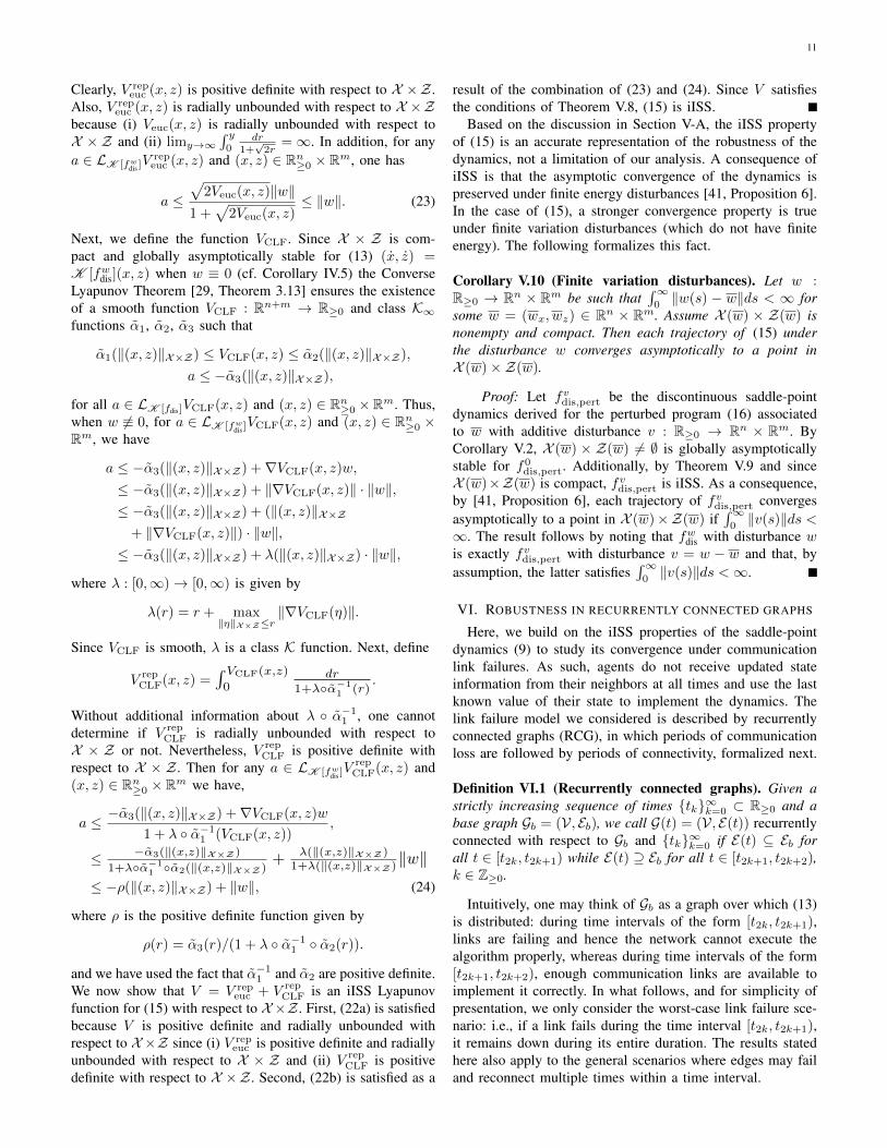
Here we illustrate the convergence and robustness propertiesof the discontinuous saddle-point dynamics. We consider afinite-horizon optimal control problem for a network of agentswith coupled dynamics and underactuation. The network-widedynamics is open-loop unstable and the aim of the agents is tofind a control to minimize the actuation effort and ensure thenetwork state remains small. To achieve this goal, the agentsuse the discontinuous saddle-point dynamics (13). Formally,consider the finite-horizon optimal control problem,

min

T∑τ=0

‖x(τ + 1)‖1 + ‖u(τ)‖1 (27a)

s.t. x(τ + 1) = Gx(τ) +Hu(τ), τ = 0, . . . T, (27b)

where x(τ) ∈ RN and u(τ) ∈ RN is the network stateand control, respectively, at time τ . The initial point xi(0) isknown to agent i and its neighbors. The matrices G ∈ RN×Nand H = diag(h) ∈ RN×N , h ∈ RN , define the networkevolution, and the network topology is encoded in the sparsitystructure of G. We interpret each agent as a subsystem whosedynamics is influenced by the states of neighboring agents.An agent knows the dynamics of its own subsystem and itsneighbor’s subsystem, but does not know the entire networkdynamics. A solution to (27) is a time history of optimalcontrols (u∗(0), . . . , u∗(T )) ∈ (RN )T .

To express this problem in standard linear programmingform (4), we split the states into their positive and negativecomponents, x(τ) = x+(τ)− x−(τ), with x+(τ), x−(τ) ≥ 0(and similarly for the inputs u(τ)). Then, (27) can be equiva-lently formulated as the following linear program,

min

T∑τ=0

N∑i=1

x+i (τ + 1)+x−i (τ + 1)+u+i (τ)+u−i (τ) (28a)

s.t. x+(τ + 1)− x−(τ) = G(x+(τ)− x−(τ))

+H(u+(τ)− u−(τ)), τ = 0, . . . , T (28b)x+(τ + 1), x−(τ + 1), u+(τ), u−(τ) ≥ 0, ∀τ (28c)

The optimal control for (27) at time τ is then u∗(τ) = u+∗ (τ)−u−∗ (τ), where the vector (u+∗ (0), u−∗ (0), . . . , u+∗ (T ), u−∗ (T ))is a solution to (28), cf. [42, Lemma 6.1].

We implement the discontinuous saddle-point dynamics (13)for problem (28) over the network of 5 agents described inFigure 2. To implement the dynamics (13), neighboring agentsmust exchange their state information with each other. In thisexample, each agent is responsible for 2(T+1) = 24 variables,which is independent of the network size. This is in contrastto consensus-based distributed optimization algorithms, whereeach agent would be responsible for 2N(T + 1) = 120variables, which grows linearly with the network size N .For simulation purposes, we implement the dynamics as asingle program in MATLAB R©, using a first-order (Euler)

approximation of the differential equation with a stepsize of0.01. The CPU time for the simulation is 3.1824s on a 64-bit 3GHz Intel R© CoreTM i7-3540M processor with 16GB ofinstalled RAM.

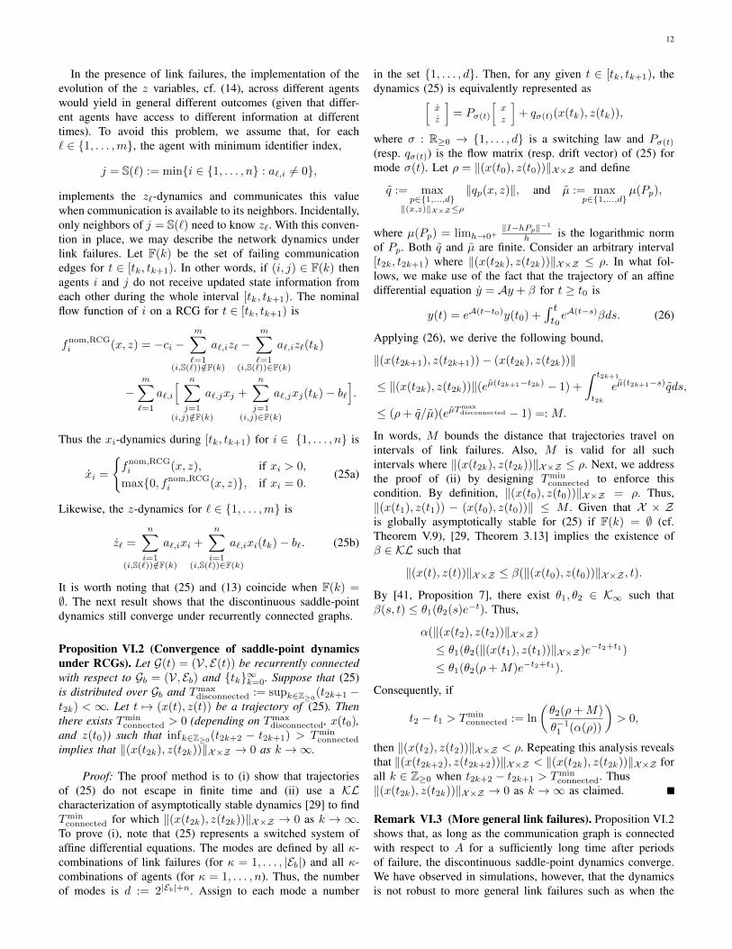
Note that, when implementing this dynamics, agent i ∈1, . . . , 5 computes the time history of its optimal control,u−i (0), u+i (0), . . . , u−i (T ), u+i (T ), as well as the time historyof its states, x−i (1), x+i (1), . . . , x−i (T + 1), x+i (T + 1). Withrespect to the solution of the optimal control problem, thetime history of states are auxiliary variables used in thediscontinuous dynamics and can be discarded after the controlis determined. Figure 3 shows the results of the implementa-tion of (13) when a finite energy noise signal disturbs theagents’ execution. Clearly (13) achieves convergence initiallyin the absence of noise. Then, the finite energy noise signalin Figure 3(b) enters each agents’ dynamics and disruptsthis convergence, albeit not significantly due to the iISSproperty of (15) characterized in Theorem V.9. Once the noisedisappears in the agents’ computation of its optimal control,convergence of the algorithm ensues. The constraint violationis plotted in Figure 3(c). Once the time history of optimalcontrols has been computed (corresponding to the steady-statevalues in Figure 3(a)), agent 1 implements it, and the resultingnetwork evolution is displayed in Figure 3(d). Agent 1 isable to drive the system state to zero, despite it being open-loop unstable. Figure 4 shows the results of implementationin a recurrently connected communication graph and (13) stillachieves convergence as characterized in Proposition VI.2. Thelink failure model here is a random number of random linksfailing during times of disconnection. The graph is repeatedlyconnected for 1s and then disconnected for 4s (i.e., the ratioTmaxdisconnected : Tmin

connected is 4 : 1). The fact that convergence isstill achieved under this unfavorable ratio highlights the strongrobustness properties of the algorithm.

VIII. CONCLUSIONS

We have considered a network of agents whose objec-tive is to have the aggregate of their states converge toa solution of a general linear program. We proposed anequivalent formulation of this problem in terms of findingthe saddle points of a modified Lagrangian function. To makean exact correspondence between the solutions of the linearprogram and saddle points of the Lagrangian we incorporatea nonsmooth penalty term. This formulation has naturallyled us to study the associated saddle-point dynamics, forwhich we established the point-wise convergence to the setof solutions of the linear program. Based on this analysis,we introduced an alternative algorithmic solution with thesame asymptotic convergence properties. This dynamics isamenable to distributed implementation over a multi-agentsystem, where each individual controls its own component ofthe solution vector and shares its value with its neighbors.We also studied the robustness against disturbances and linkfailures of this dynamics. We showed that it is integral-input-to-state stable but not input-to-state stable (and, in fact, noalgorithmic solution for linear programming is). These resultshave allowed us to formally establish the resilience of our

14

x(τ + 1) =

2

6

6

6

6

4

0.5 0 0 0 0.70.7 0.5 0 0 00 0.7 0.5 0 00 0 0.7 0.5 00 0 0 0.7 0.5

3

7

7

7

7

5

x(τ ) + diag

0

B

B

B

B

@

2

6

6

6

6

4

10000

3

7

7

7

7

5

1

C

C

C

C

A

u(τ )

(a) Network dynamics

x1

x2x5

x4 x3

= node withactuation

(b) Communication topology

Fig. 2. Network dynamics and communication topology of the multi-agent system. The network dynamics is underactuated and open-loop unstable butcontrollable. The presence of a communication link in (b) among every pair of agents whose dynamics are coupled in (a) ensures that the algorithm (13) isdistributed over the communication graph.

−4

−3

−2

−1

0

1

2

3

4

5

6

Time, t

Agent

1’s

contr

ol

u1(0

),...,

u1(1

1)

(a) Computing the optimal control (with noise)

−5

−4

−3

−2

−1

0

1

2

3

4

5

Time, tN

ois

e,

w(t

)

(b) Finite energy noise used in (a)

0

1

2

3

4

5

Time, t

ConstraintViolation,

||Ax−

b||

→

0

1

2

3x 10−3

(c) Equality constraint violation in (a)

2 4 6 8 10 12−7

−6

−5

−4

−3

−2

−1

0

1

2

3

4

Time step, τ

x(τ

)

(d) Network evolution under optimal control found in (a)

Fig. 3. Plot (a) shows the trajectories of the discontinuous saddle-point dynamics (15) subject to the noise depicted in (b) for agent 1 as it computes itstime history of optimal controls. Plot (c) shows the associated equality constraint violation. The asymptotic convergence of the trajectories appears to beexponential. The time horizon of the optimal control problem (28) is T = 11. The 12 trajectories in (a) and (b) represent agent 1’s evolving estimates ofthe optimal controls u1(0), . . . , u1(11). The steady-state values achieved by these trajectories correspond to the solution of (27). Once determined, thesecontrols are then implemented by agent 1 and result in the network evolution depicted in (d). The dynamics is initialized to a random point.

distributed dynamics to disturbances of finite variation andrecurrently disconnected communication graphs. Future workwill include the study of the convergence rate of the dynamicsand its robustness properties under more general link failures,the synthesis of continuous-time computation models withopportunistic discrete-time communication among agents, andthe extension of our design to other convex optimizationproblems. We also plan to explore the benefits of the proposeddistributed dynamics in a number of engineering scenarios,including the smart grid and power distribution, bargainingand matching in networks, and model predictive control.

ACKNOWLEDGMENTS

The authors would like to acknowledge helpful commentsfrom Simon Niederlaender, in particular regarding the proofs

of Theorem IV.1 and Corollary IV.2. This research was sup-ported by Award FA9550-10-1-0499 and NSF award CMMI-1300272.

REFERENCES

[1] R. Alberton, R. Carli, A. Cenedese, and L. Schenato, “Multi-agentperimeter patrolling subject to mobility constraints,” in American Con-trol Conference, (Montreal), pp. 4498–4503, 2012.

[2] D. P. Bertsekas, Network Optimization: Continuous and Discrete Mod-els. Athena Scientific, 1998.

[3] M. Ji, S. Azuma, and M. Egerstedt, “Role-assignment in multi-agentcoordination,” International Journal of Assistive Robotics and Mecha-tronics, vol. 7, no. 1, pp. 32–40, 2006.

[4] B. W. Carabelli, A. Benzing, F. Durr, B. Koldehofe, K. Rothermel,G. Seyboth, R. Blind, M. Burger, and F. Allgower, “Exact convexformulations of network-oriented optimal operator placement,” in IEEEConf. on Decision and Control, (Maui), pp. 3777–3782, Dec. 2012.

15

[5] D. R. Kuehn and J. Porter, “The application of linear programmingtechniques in process control,” IEEE Transactions on Applications andIndustry, vol. 83, no. 75, pp. 423–427, 1964.

[6] J. Trdlicka, Z. Hanzalek, and M. Johansson, “Optimal flow routingin multi-hop sensor networks with real-time constraints through linearprogramming,” in IEEE Conf. on Emerging Tech. and Factory Auto.,pp. 924–931, 2007.

[7] W. F. Sharpe, “A linear programming algorithm for mutual fund portfolioselection,” Management Science, vol. 13, no. 7, pp. 499–510, 1967.

[8] G. B. Dantzig, Linear Programming and Extensions. Princeton, NJ:Princeton University Press, 1963.

[9] D. Bertsimas and J. N. Tsitsiklis, Introduction to Linear Optimization,vol. 6 of Optimization and Neural Computation. Belmont, MA: AthenaScientific, 1997.

[10] S. Boyd and L. Vandenberghe, Convex Optimization. CambridgeUniversity Press, 2009.

[11] M. Burger, G. Notarstefano, F. Bullo, and F. Allgower, “A distributedsimplex algorithm for degenerate linear programs and multi-agent as-signment,” Automatica, vol. 48, no. 9, pp. 2298–2304, 2012.

[12] G. Notarstefano and F. Bullo, “Distributed abstract optimization viaconstraints consensus: Theory and applications,” IEEE Transactions onAutomatic Control, vol. 56, no. 10, pp. 2247–2261, 2011.

[13] G. Yarmish and R. Slyke, “A distributed, scalable simplex method,”Journal of Supercomputing, vol. 49, no. 3, pp. 373–381, 2009.

[14] A. Nedic, A. Ozdaglar, and P. A. Parrilo, “Constrained consensus andoptimization in multi-agent networks,” IEEE Transactions on AutomaticControl, vol. 55, no. 4, pp. 922–938, 2010.

[15] M. Zhu and S. Martınez, “On distributed convex optimization underinequality and equality constraints,” IEEE Transactions on AutomaticControl, vol. 57, no. 1, pp. 151–164, 2012.

[16] J. Wang and N. Elia, “A control perspective for centralized and dis-tributed convex optimization,” in IEEE Conf. on Decision and Control,(Orlando, Florida), pp. 3800–3805, 2011.

[17] R. Olfati-Saber, J. A. Fax, and R. M. Murray, “Consensus and coop-eration in networked multi-agent systems,” Proceedings of the IEEE,vol. 95, no. 1, pp. 215–233, 2007.

[18] W. Ren and R. W. Beard, Distributed Consensus in Multi-Vehicle Co-operative Control. Communications and Control Engineering, Springer,2008.

[19] F. Bullo, J. Cortes, and S. Martınez, Distributed Control of RoboticNetworks. Applied Mathematics Series, Princeton University Press,2009. Electronically available at http://coordinationbook.info.

[20] M. Mesbahi and M. Egerstedt, Graph Theoretic Methods in MultiagentNetworks. Applied Mathematics Series, Princeton University Press,2010.

[21] R. Carli and G. Notarstefano, “Distributed partition-based optimizationvia dual decomposition,” in IEEE Conf. on Decision and Control,(Firenze), pp. 2979–2984, Dec. 2013.

[22] D. P. Bertsekas and J. N. Tsitsiklis, Parallel and Distributed Computa-tion: Numerical Methods. Athena Scientific, 1997.

[23] I. Necoara and J. Suykens, “Application of a smoothing technique todecomposition in convex optimization,” IEEE Transactions on AutomaticControl, vol. 53, no. 11, pp. 2674 – 2679, 2008.

[24] N. Garg and J. Konemann, “Faster and simpler algorithms for multi-commodity flow and other fractional packing problems,” in Proceedings

of the 39th Annual Symposium on Foundations of Computer Science,(Palo Alto, CA), pp. 300–309, 1998.

[25] V. Nedelcu, I. Necoara, and D. Quoc, “Computational complexityof inexact gradient augmented Lagrangian methods: Application toconstrained MPC,” SIAM Journal on Control and Optimization, vol. 52,no. 5, pp. 3109–3134, 2014.

[26] I. Necoara and V. Nedelcu, “Rate analysis of inexact dual first ordermethods,” IEEE Transactions on Automatic Control, vol. 59, no. 5,pp. 1232–1243, 2014.

[27] D. Feijer and F. Paganini, “Stability of primal-dual gradient dynam-ics and applications to network optimization,” Automatica, vol. 46,pp. 1974–1981, 2010.

[28] K. Arrow, L. Hurwitz, and H. Uzawa, Studies in Linear and Non-LinearProgramming. Stanford, California: Stanford University Press, 1958.

[29] C. Cai, A. R. Teel, and R. Goebel, “Smooth Lyapunov functions forhybrid systems part II: (pre)asymptotically stable compact sets,” IEEETransactions on Automatic Control, vol. 53, no. 3, pp. 734–748, 2008.

[30] E. D. Sontag, “Further facts about input to state stabilization,” IEEETransactions on Automatic Control, vol. 35, pp. 473–476, 1989.

[31] D. Angeli, E. D. Sontag, and Y. Wang, “A characterization of inte-gral input-to-state stability,” IEEE Transactions on Automatic Control,vol. 45, no. 6, pp. 1082–1097, 2000.

[32] D. Bertsimas, D. B. Brown, and C. Caramanis, “Theory and applicationsof robust optimization,” SIAM Review, vol. 53, no. 3, pp. 464–501, 2011.

[33] F. H. Clarke, Optimization and Nonsmooth Analysis. Canadian Mathe-matical Society Series of Monographs and Advanced Texts, Wiley, 1983.

[34] J. Cortes, “Discontinuous dynamical systems - a tutorial on solutions,nonsmooth analysis, and stability,” IEEE Control Systems Magazine,vol. 28, no. 3, pp. 36–73, 2008.

[35] D. P. Bertsekas, A. Nedic, and A. E. Ozdaglar, Convex Analysis andOptimization. Belmont, MA: Athena Scientific, 1st ed., 2003.

[36] R. Dorfman, P. A. Samuelson, and R. Solow, Linear programming ineconomic analysis. New York, Toronto, and London: McGraw Hill,1958.

[37] J. P. Aubin and A. Cellina, Differential Inclusions, vol. 264 ofGrundlehren der mathematischen Wissenschaften. New York: Springer,1984.

[38] W. Rudin, Principles of Mathematical Analysis. McGraw-Hill, 1953.[39] H. J. Kushner and G. G. Yin, Stochastic Approximation and Recursive

Algorithms and Applications, vol. 35 of Applications of Mathematics:Stochastic Modelling and Applied Probability. New York: Springer,2nd ed., 2003.

[40] R. J. B. Wets, “On the continuity of the value of a linear program and ofrelated polyhedral-valued multifunctions,” Mathematical ProgrammingStudy, vol. 24, pp. 14–29, 1985.

[41] E. D. Sontag, “Comments on integral variants of ISS,” Systems &Control Letters, vol. 34, no. 1-2, pp. 93–100, 1998.

[42] G. B. Dantzig, Linear Programming: 1: Introduction. New York:Springer, 1997.

[43] D. P. Bertsekas, Nonlinear Programming. Belmont, MA: AthenaScientific, 2nd ed., 1999.

−6

−4

−2

0

2

4

6

8

Time, t

u1(0

),...,

u1(1

1)

Fig. 4. The trajectories of the discontinuous saddle-point dynamics (15)under a recurrently connected communication graph where a random numberof random links failed during periods of disconnection. The simulationparameters are the same as in Figure 3.

16

APPENDIX

The following is a technical result used in the proof ofTheorem V.4.

Lemma A.1 (Property of feasible set). If Ax = b, x ≥ 0is non-empty and bounded then AT z ≥ 0 is unbounded.

Proof: We start by proving that there exists an ν ∈ Rmsuch that Ax = b + ν, x ≥ 0 is empty. Define the vectors ∈ Rn component-wise as si = maxAx=b,x≥0 xi. SinceAx = b, x ≥ 0 is compact and non-empty, s is finite. Next,fix ε > 0 and let ν = −A(s + ε1n). Note that Ax = b + νcorresponds to A(x+s+ε1n) = b, which is a shift by s+ε1nin each component of x. By construction, Ax = b + ν, x ≥0 is empty. Then, the application of Farkas’ Lemma [10,pp. 263] yields that there exists z ∈ Rm such that AT z ≥ 0and (b+ ν)T z < 0 (in particular, (b+ ν)T z < 0 implies thatz 6= 0). For any λ ∈ R≥0, it holds that AT (λz) ≥ 0, and thusλz ∈ AT z ≥ 0, which implies the result.

The proof of Theorem V.9 makes use of the following resultfrom [43, Proposition B.25].

Theorem A.2 (Danskin’s Theorem). Let Y ⊂ Rm be com-pact and convex. Given g : Rn × Y → R, suppose thatx 7→ g(x, y) is differentiable for every y ∈ Y , ∂xg iscontinuous on Rn × Y , and y 7→ g(x, y) is strictly convexand continuous for every x ∈ Rn. Define f : Rn → R byf(x) = miny∈Y g(x, y). Then, ∇f(x) = ∂xg(x, y)|y=y∗(x),where y∗(x) = argminy∈Y g(x, y).

Dean Richert received the B.Sc. and M.Sc. degreein electrical and computer engineering from theUniversity of Calgary, Canada, in 2008 and 2010respectively. In 2014, he received the Ph.D. degreein mechanical and aerospace engineering at the Uni-versity of California, San Diego (UCSD). He was therecipient of a Jacob’s Fellowship from UCSD as wellas a Postgraduate Scholarship from the Natural Sci-ences and Engineering Research Council of Canada.His research interests include cooperative control,distributed optimization, game theory, nonsmooth

analysis, and set-valued dynamical systems. Currently, Dean works as a Sr.Algorithms Engineer at Cymer, Inc. (an ASML company).

Jorge Cortes received the Licenciatura degreein mathematics from Universidad de Zaragoza,Zaragoza, Spain, in 1997, and the Ph.D. degree inengineering mathematics from Universidad CarlosIII de Madrid, Madrid, Spain, in 2001. He held post-doctoral positions with the University of Twente,Twente, The Netherlands, and the University ofIllinois at Urbana-Champaign, Urbana, IL, USA. Hewas an Assistant Professor with the Department ofApplied Mathematics and Statistics, University ofCalifornia, Santa Cruz, CA, USA, from 2004 to

2007. He is currently a Professor in the Department of Mechanical andAerospace Engineering, University of California, San Diego, CA, USA. Heis the author of Geometric, Control and Numerical Aspects of NonholonomicSystems (Springer-Verlag, 2002) and co-author (together with F. Bullo and S.Martınez) of Distributed Control of Robotic Networks (Princeton UniversityPress, 2009). He is an IEEE Fellow and an IEEE Control Systems SocietyDistinguished Lecturer. His current research interests include distributedcontrol, networked games, power networks, distributed optimization, spatialestimation, and geometric mechanics.