Robust design of Bridges

- Robustness analysis of Sjölundaviadukt Bridge

Ívar Björnsson

Division of Structural Engineering Lund Institute of Technology Lund University, 2010

Report TVBK - 5179

i

Avdelningen för Konstruktionsteknik Lunds Tekniska Högskola Box 118 221 00 LUND Department of Structural Engineering Lund Institute of Technology Box 118 S-221 00 LUND Sweden Robust design of bridges - Robustness analysis of Sjölundaviadukten Bridge in Malmö Robust utforming av broar - En robusthetsstudie av Sjölundaviadukten i Malmö Ívar Björnsson 2010

Abstract

Robustness of structural systems is as yet not explicitly defined nor is there a clearly defined method for incorporating robustness in design/construction. Robustness can be simply defined as the ability of a structural system to survive unforeseen/extraordinary exposures or circumstances that would otherwise cause it to fail. The structure must have enough residual capacity during and after the event to maintain at least some of its intended function intact. The level of robustness of a structure has to be analyzed in terms of the causes and consequences of failure; i.e. the consequences of structural damages should not be disproportional to the original cause (see 2.1 (3) of EN 1990:2002). This master thesis deals with the robustness of bridge structures. It examines common circumstances of failure and investigates methods and strategies towards incorporating structural robustness into the design of bridges. A robustness analysis is conducted for the Sjölundaviadukten Bridge; a 5-span post-tensioned frame bridge in Malmö.

Keywords: bridges; collapse; robustness; design; strategies; accidental circumstances; train derailment; probabilistic methods; failure progression

ii

Report no. TVBK-5179 ISSN 0349-4969 ISRN: LUTVDG/TVBK-10/5179+113p Master Thesis Supervisor: Dr. Fredrik Carlsson Examinator: Prof. Sven Thelandersson March 2010 Front Cover: Picture of I-35 Bridge Collapse in Minneapolis, 1st Aug. 2007. Photo taken by Kevin Rofidal, United States Coast Guard. Downloaded 2010-03: http://en.wikipedia.org/wiki/I-35W_Mississippi_River_bridge

iii

Foreword

This master thesis was completed under the administration of the Division of Structural Engineering at the University of Lund. It was initiated in September 2009, under the supervision of Professor Sven Thelandersson and Dr. Fredrik Carlsson. The work presented in this thesis is intended as an inaugural effort for the research project which was initiated by the Vägverket in 2009 under the official title: “Robust bridge design for reduced vulnerability in the road transport system.”

The completion of this thesis marks the end of my academic tenure as a master student at the Lund Institute of Technology. My only hope is that the reader obtains a deeper understanding of the issues related to the topic than I had when I first started my research.

Acknowledgements

I want to express my deepest thanks to all of those involved in the creation of this work. I would especially like to extend my thanks to Sven Thelandersson and Fredrik Carlsson for their skillful guidance and expertise, Magnus Gilliam and Kristoffer Larsson from Centerlof & Holmberg for all their help and patience, and Ebbe Rossel from Vägverket for his input. I would also like to thank the Department of Structural Engineering at Lund University for allowing me to work among them, Centerlof & Holmberg for allowing me to examine their bridge and the Vägverket for allowing me to work on this project. And to anyone with whom I’ve had fruitful discussions about this project, I thank you for your input.

Lund, March 2010 Ívar Björnsson

“A person filled with gumption doesn't sit about stewing about things. He's at the front of the train of his own awareness, watching to see what's up the track and meeting it when it comes. That's gumption. If you're going to repair a motorcycle, an adequate supply of gumption is the first and most important tool. If you haven't got that you might as well gather up all the other tools and put them away, because they won't do you any good.”

- Robert M. Pirsig (Zen and the art of motorcycle maintenance)

iv

v

Table of Contents

1. Introduction ....................................................................................................................... 1

1.1 Background .................................................................................................................. 1

1.2 Objectives .................................................................................................................... 2

1.3 Outline of the thesis ..................................................................................................... 2

2. Robustness ......................................................................................................................... 3

2.1 Introduction ................................................................................................................. 3

2.2 Robustness in engineering ........................................................................................... 3

2.3 What is structural robustness? ..................................................................................... 4

2.4 Robustness in design ................................................................................................... 6

2.4.1 Current design methods .................................................................................... 6

2.4.2 Robustness through design ............................................................................... 7

2.5 Robustness of bridges .................................................................................................. 8

3. Circumstances for failure ............................................................................................... 11

3.1 General overview ....................................................................................................... 11

3.2 Internal flaws ............................................................................................................. 12

3.3 External exposures ..................................................................................................... 13

3.4 Hierarchy of failure modes ........................................................................................ 14

4. Consequences of failure .................................................................................................. 17

4.1 Consequences to structural system ............................................................................ 17

4.2 Consequences to super-system .................................................................................. 20

5. Strategies & methods of Robustness ............................................................................. 21

5.1 Introduction ............................................................................................................... 21

5.2 Methods for quantification of Robustness ................................................................. 21

5.2.1 Based on structural behavior .......................................................................... 22 5.2.1.1 Probabilisticmeasures ............................................................................. 22 5.2.1.2 Deterministic measures ........................................................................... 23

5.2.2 Based on structural attributes ......................................................................... 24

5.2.3 Robustness Index ............................................................................................ 24

5.3 Strategies towards greater Robustness of Bridges ..................................................... 26

5.3.1 Prevent local failure of critical elements: first line of defense ....................... 26

5.3.2 Assume local failure: Second line of defense ................................................. 27 5.3.2.1 Multiple load paths or redundancy ......................................................... 27 5.3.2.2 Knock-out scenario ................................................................................. 29 5.3.2.3 Segmentation ........................................................................................... 29

5.3.3 Prescriptive design rules ................................................................................. 30

vi

6. Robustness considerations of Sjölundaviadukten Bridge ........................................... 31

6.1 Introduction ............................................................................................................... 31

6.2 Background ................................................................................................................ 32

6.3 Structural system ....................................................................................................... 33

6.3.1 Specifications/assumptions ............................................................................ 36 6.3.1.1 Bridge Structure ...................................................................................... 36 6.3.1.2 Road traffic ............................................................................................. 37 6.3.1.3 Rail tracks & railway traffic ................................................................... 37

6.4 Hazard scenarios ........................................................................................................ 39

6.5 Method of analysis ..................................................................................................... 41

6.6 Pylon collision due to train derailment ...................................................................... 43

6.6.1 Probability of train derailment in direction towards support ......................... 46

6.6.2 Direct consequences of pylon collision .......................................................... 53 6.6.2.1 Action effect – force from collision ......................................................... 53 6.6.2.2 Resistance of support .............................................................................. 58 6.6.2.3 Probability of pylon failure given train derailment towards support ..... 64

6.6.3 Indirect consequences of pylon collision ....................................................... 70

6.7 Summary of results .................................................................................................... 77

6.8 Alternative robust solutions ....................................................................................... 79

7. Conclusions and Discussion ............................................................................................ 81

8. References ........................................................................................................................ 83

Appendix A. Train derailment – simplified model ............................................................ 87

A.1 Mechanics of derailment ........................................................................................... 87

A.1.1 Velocity at impact .......................................................................................... 88

A.1.2 Force at impact ............................................................................................... 89

A.2 Maximum derailment angle, θmax .............................................................................. 90

A.2.1 Statistical parameters for θmax ........................................................................ 91

A.3 Minimum derailment angle, θmin ............................................................................... 92

A.3.1 Statistical parameters for θmin ......................................................................... 92

A.4 Critical region for derailment, xcrit ............................................................................. 95

A.4.1 Statistical parameters for xcrit ......................................................................... 95

Appendix B. Probability of derailment ............................................................................... 99

B.1 Model for probability calculations of train accidents in Sweden .............................. 99

B.2 Train derailment near Sjölundavaidukt Bridge ....................................................... 101

Appendix C. Resistance of support wall ........................................................................... 103

C.1 Moment-Normal force graph ................................................................................... 103

Appendix D. Capacity of bridge deck ............................................................................... 107

1

1. Introduction

1.1 Background The concept of a bridge could be conjectured to have existed during even the earliest days of man; early hunters and gatherers might have used local materials such as fallen trees to cross streams or small ravines. Latter day engineering developments such as the invention of the structural arch form by the Romans around the first century A.D., however, paved way for the modern day concept of a bridge. Since then, bridges have developed into various forms that are able to span greater distances and have greater carrying capacities. Technological advances have allowed man to create, analyze and construct more complex and grander structural bridge systems which are, ironically, seemingly even more vulnerable than the bridges of old; some of which still stand today.

Presently, bridges are designed and constructed to endure what is considered normal use for the duration of the structures intended lifetime. This usually only includes foreseeable circumstances and exposures expected to occur during the bridges lifespan while low probability events are neglected. However, there is always some chance that something extraordinary will occur which was either unanticipated or underestimated resulting in bridge failure and possibly human casualties. These circumstances can be very diverse and may be hard to foresee beforehand, but must not be ignored.

There has been increased research towards understanding the reasons behind failure and progressive collapse of bridges during the past decades through forensic engineering. The questions that are being asked are: how and why did this happen; could it have been prevented; and whose fault is it? It is possible to investigate collapsed bridge sites after-the-fact in an effort to understand the reasons behind the failure, however, it is often more difficult to try and foresee these circumstances during the design and planning of the bridge; hindsight is, as always, 100%. A well known example is the Tacoma Narrows Bridge which collapsed in 1940 due to torsional oscillations of the bridge deck stiffening girder caused by dynamic effects from wind loading; i.e. vortex shedding. At that time, knowledge of aerodynamic phenomena such as wind induced vibrations was not as well developed scientifically nor was it as widely known as it is today1; at least not within bridge engineering circles that put emphasis on static-load carrying capacity while neglecting the effects of dynamics (in fact, the bridge was designed to withstand static wind pressure for wind speeds almost three times more than recorded when it collapsed). According to Theodore v. Kármán, an engineer/physicist who sat on the federal committee chosen to investigate the failure of the bridge, “…the sessions … ended with most of the committee convinced of the worth of the new science of aerodynamics in bridge building.” [1] The bridge’s slender and flexible stiffening girder was not robust enough to endure the aerodynamic effects caused by the wind and this omission in its design was the reason for the collapse.

1 Collapse of bridges due to vibration caused by winds was not, however, unknown; for example, the Wheeling Bridge in 1849. See Åkesson 2008 pp. 97-114.

2

The fact remains that bridges have been known to fail due to unexpected or unusual circumstances and the significance of these failures must not be taken lightly. The ability of a bridge, or structure in general, to survive these circumstances, at least to the extent where casualties can be prevented, is referred to as structural robustness; a structural property which must be taken into consideration when designing and building a structure.

1.2 Objectives The main objective of this thesis is two-fold: (1) to examine and investigate robustness of bridge structures in general including circumstances of failure, consequences of collapse, methods of quantifying robustness and strategies toward greater structural robustness; and (2) a basic analysis of the Sjölundaviadukt Bridge, a 5 span post tensioned concrete bridge in Malmö, in terms of its structural robustness incorporating the points of discussion from the aforementioned objective. In this way a blue print towards incorporating robustness in the design and investigation of bridges can be developed.

1.3 Outline of the thesis Chapter 2 discusses the topic of structural robustness in modern day engineering including issues of designing structures for robustness. This chapter gives a background to different aspects of robustness and its relevance to bridge structures.

Chapter 3 defines a set of extraordinary exposures that are common circumstances for failure of bridges. It includes a general overview of circumstances in which limit state bridge design is no longer adequate to the survival of the structure and in which structural robustness becomes paramount.

Chapter 4 discusses the various consequences of failure due to the exposures discussed in chapter 3 in terms of structural and safety considerations as well as its impact on the surrounding infrastructure.

Chapter 5 deals with various strategies and methods towards quantifying robustness as well as attaining greater structural robustness in bridges.

Chapter 6 is an investigation of the structural robustness of the Sjölundaviadukt Bridge in Malmö. The bridge will be analyzed in terms of the relevant exposures and consequences based on chapters 3 and 4, which also include a discussion of possible alternative solutions which may serve to increase robustness (regarding the strategies and methods discussed in chapter 5).

Chapter 7 is a summary and discussion of results from previous chapters

3

2. Robustness

2.1 Introduction The term robustness is defined in the Oxford English Dictionary as something or someone having a “robust character or quality”2. The word robust is synonymous with strength and resilience; from Latin rōbustus, from rōbur meaning strength. This makes sense in a colloquial dictum when referring to, for example, a person’s build or a full-bodied wine, but its usage is quite ambiguous with regard to “engineering terminology”. In reference to the latter, terms such as strength and resilience require a more quantitative description as well as a specific association; for example, a concrete reinforced beam can be described in terms of its flexural strength, or more notably, its resistance to external loading. The following sections aim to more clearly define what is referred to as structural robustness and its application within structural engineering and more specifically, for bridge structures.

2.2 Robustness in engineering Robustness can have various meanings in differing fields of science and technology including statistical or probabilistic investigation/interpretation, pharmaceutical procedure, ecological systems, genetics, and software development to name a few. Typically the general scientific interpretation of robustness can broadly be defined as the manner in which a “system” is affected by hazardous/extreme or varying procedures or circumstances. However, in order to measure and rank the degree of robustness of a specific system, certain elements must first be clarified (Maes et. al. 2006):

1. The system must be clearly defined. 2. The intended functions/objectives of the system must be identified. 3. The perturbations (eg. hazards, endogenous an exogenous circumstances, deviations

from design assumptions, etc.) which affect the system are identified. 4. The overall consequences of individual perturbations are analyzed with regard to the

aforementioned functions/objectives. 5. The level of robustness can then be obtained and ranked with all this in mind3.

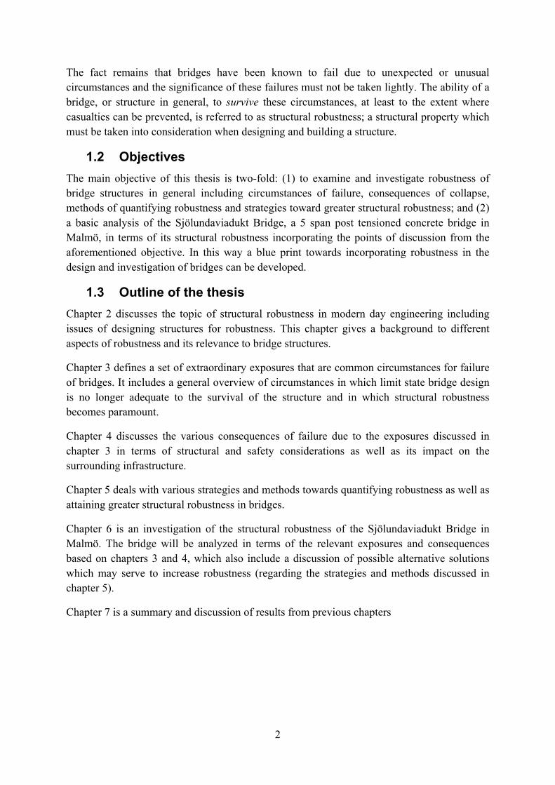
The resulting robustness is unique to that system alone and cannot be applied generally to other systems. Refer to figure 2.1 for a schematic for the process of assessing robustness.

2 Oxford English Dictionary <www.oed.com> 3 Methods of ranking robustness are discussed in section 5

4

Figure 2.1 Schematic of the process of assessing robustness (Maes et al. 2006)

It is important to note that some of the input parameters utilized for a robustness assessment may be assumed or contain uncertainties which also need to be taken into account during analysis; this is referred to as risk.

The aforementioned interpretation of robustness and its assessment can be applied within engineering but an explicit definition specific to structures is still lacking. Thus, robustness as a property within structural engineering systems will be, for the purposes of clarification, referred to as structural robustness.

2.3 What is structural robustness? The partial collapse of the Ronan Point Tower in east London due to a gas explosion in May 1968 was when the robustness of structures first received significant attention within the engineering community. It prompted much research towards implementing counter-measures against progressive collapse in buildings and enhancing overall structural integrity as well as introducing design requirements for accidental loading into the UK Codes of Practice and regulatory requirements in the early 1970s; one of the earliest examples of regulations of this kind being included in structural or building codes (Gulvanessian et al. 2006). However, there has since been a revival of interest in structural robustness as well as an increase of internationally funded research following recent terrorist attacks including the collapse of the WTC on September 11, 2001. A good example of this is the EU COST (European Cooperation in Science and Technology) action TU 0601 [2], initiated in 2007 by the JCSS (Joint Committee on Structural Safety), which “…aims to develop a foundation for treatment of structural robustness in future structural design codes. “ [3]

Despite this increased attention towards structural robustness there is as yet no consensus as to a universal interpretation of structural robustness nor is there an explicit framework for its application in design and execution. However, something that everybody seems to agree upon is that unanticipated or progressive collapse should be avoided; one way of doing this is through structural robustness.

5

The European building standard Eurocode defines robustness as: “the ability of a structure to withstand events like fire, explosions, impact or the consequences of human error, without being damaged to an extent disproportionate to the original cause.” (prEN1991-1-7:2003) Similar definitions are given by other building standards around the world including in Denmark, Switzerland and Italy. The following definitions of structural robustness and progressive collapse will be used for the purposes of this paper.

Structural robustness:

Structural robustness is the property of a structural system which enables it to survive extraordinary exposures and circumstances, beyond the scope of conventional design criteria, without disproportional1 damage or loss of function.

1- The degree of acceptable disproportion should be prescribed in the design requirements for the structural system being analyzed

As an addition to the above definition the terms structural system and survival need to be clarified.

Structural system:

It is difficult to state a short and concise definition of a structural system. A complex theoretical interpretation of a system has been developed by G. Ropohl in Systems Theory of Engineering (1979). It combines functional, structural and hierarchical concepts of a system and is valid for deterministic, stochastic, dynamic and static systems (Stempfle et al. 2005). A general definition will be formulated with basis on Stempfle et al. (2005):

A structural system is the complex composition of a variety of subsystems whose attributes, functionality and interrelations constitute the overall structural system. The interactions between the subsystems and the factors which influence them constitute the entire system. The set of subsystems are defined in the same way as the parent system with their own subsystems and thus creating a hierarchy of systems. The lowest level of subsystems within the hierarchy is defined as an element; the degree of segmentation is dependent on the type of analysis being done. The structural system is limited in time, space and purpose.

The structural system in this case refers not only to the physical bridge structure but also external influences including relevant perturbations (such as loading, fatigue, deterioration, etc.), inspection procedures, maintenance and reparations during the structures lifetime.

A structural system can be categorized into two fundament types (JCSS Probabilistic model code 2001):

1. Series system: system fails if one or more of its components fail 2. Parallel system: system fails when all of its components fail

6

Survival:

In terms of structural robustness, the term survival refers to the preservation of the intended function of the structure regardless of circumstance. This may include limited damage or a reduction/loss of function limited in time (Knoll et al. 2009).

NOTE: Robustness can also be defined as a structure’s insensitivity to local failure (Starossek 2009) and is thus a property of the structure alone independent of possible causes of initial local failure.

Progressive collapse:

Progressive collapse is characterized by a disproportion in size between a damaging exposure event and the resulting collapse (Starossek 2009).

A significant aspect of structural robustness is the insensitivity of a structure to progressive collapse.

2.4 Robustness in design

2.4.1 Current design methods Structural systems are usually designed to survive a set of foreseeable circumstances, which may be expected to occur, to a certain degree or magnitude, during the structure’s service lifetime; i.e. a list of anticipated exposure and events given by structural and building codes. Modern day design codes are based on structural reliability theory utilizing a framework of probabilistic-based design in which an acceptable probability of failure (or margin of safety) is decided by code committees (Melchers 1999). In simple terms, this is done by modeling statistical distributions to represent an action effect S and the corresponding resistance R; these distributions are based on samples of collected data, typically of the order of 25-50 years (Ellingwood 2001). The margin of safety is defined as the difference between these two distributions, Z = R – S. The probability of failure is then:

( ) ( ) ( )∫=<= dxxfxFZPp SRf 0 (2.1)

where ( )xFR is the cumulative distribution function of the resistance R and ( )xfS is the probability density function of action effect S.

In order to manage risks, such as unfavorable deviations or inaccurate assessments of actions or resistances, modern structural standards introduce so called safety factors, γ , into the design equations; these are also based on structural reliability theory. This can simply be represented in the following form:

∑ ⋅> niSiRn SR γγ/ (2.2)

in which both the resistance and action effects are specified conservatively.

7

There is, however, an inadequacy of current design methods with regard to structural robustness. There are three main reasons for this (Starossek 2006). Firstly, structural codes focus on component based design at a local level and thus fail to address the safety of the structural system as a whole; i.e. they do not take into account system responses to local failure. Secondly, unforeseen or improbable actions are not taken into account since supporting empirical data is unavailable. This is significant for non-robust structures where the combined low probabilities of local failure may lead to unacceptably high probabilities of global failure. Finally, structural reliability theory depends on specified acceptable probabilities of failure which are difficult to adjust with regard to disproportionate collapse. Taking into account the extreme consequences of low probability events associated with progressive collapse it is difficult to derive an acceptable failure probability.

Thus, it seems that structural robustness cannot be fully achieved using current reliability based approaches. The current design methods should rather be complemented by additional measures with particular focus on creating more robust structures.

2.4.2 Robustness through design Some modern day building code, including Eurocode, require that a structural system be robust but do not offer much in the way of aiding the engineer with achieving this demand. This, of course, allows for much interpretation on the part of the engineer as to what exactly has to be done with regard to robust design.

For example, EN 1990:2002 (Basis of structural design), clause 2.1, has this to say regarding structural robustness:

“(4)P A structure shall be designed and executed in such a way that it will not be damaged by events such as :

‐ explosions ‐ impact, and ‐ the consequences of human errors,

to an extent disproportionate to the original cause.

(5)P Potential damage shall be avoided or limited by appropriate choice of one or more of the following :

‐ avoiding, eliminating or reducing the hazards to which the structure can be subjected; ‐ selecting a structural form which has low sensitivity to the hazards considered; ‐ selecting a structural form and design that can survive adequately the accidental

removal of an individual member or a limited part of the structure, or the occurrence of acceptable localized damage;

‐ avoiding as far as possible structural systems that can collapse without warning; ‐ tying the structural members together.”

Although the above requirements do include some prescriptive design requirements as to how a structure in general may be indirectly designed to try and avoid disproportionate failure

8

(such as tying structural members) it seems to rather state the demand for a robustly designed structural system while leaving much interpretation as to its implementation for specific types of structures. Elements, strategies and methods towards structural robustness have recently been reviewed by Knoll and Vogel (2009).

A significant problem with incorporating robustness into current design methods is the need for some measure of quantification of robustness of structural systems. Otherwise the term only lends itself to subjective and almost philosophical interpretation. If a framework for the quantification of robustness can be explicitly established (and accepted), then certain limitations can be introduced with regard to ensuring structural robustness during design; i.e. an acceptable limit of disproportionality between consequences of damage and exposures is established. Currently there exist various methods of quantifying structural robustness; refer to section 5 for an overview. These recently developed approaches towards robust design, however, remain scattered and can be quite ambiguous at times (Knoll et al. 2009). Furthermore, only a few of these methods can be applied to bridges and seem to focus rather on building structures.

2.5 Robustness of bridges Prior to considering robustness in the design of any structure, the significance of the failure or malfunction of that structure must be accounted for; i.e. is structural robustness necessary and if so, to what degree. It is important to incorporate this within the specified design requirements of the structure in question. The consequences of collapse with regard to material and immaterial losses, safety, direct effects to the surrounding infrastructure and additional effects must be accounted for (Starossek 2006). Thus, the first step needed before robustness of bridges can be investigated is to establish whether there is a need for robust design of bridges. There are, of course, varying requirements of robustness depending on the bridge being investigated

Arbitrarily, a bridge is a structural system required to span a physical obstacle such as a valley, river, road, etc., providing a passage between two points. Bridges usually transport people or materials in one form or another between these two points and may also act as “tunnels” for passage under its span. The consequence of the collapse of a bridge is significant in the fact that the safety of its users may be compromised but also that the surrounding infrastructure object that are reliant on the bridge will be directly affected; not to mention the costs associated with collapse. In light of these effects, it seems obvious that bridge structures are required to be robust.

There exists a problem nowadays with the ability to try and foresee possible changes of structural demands in bridges over their long service life (Stempfle et al. 2005). Traffic demands are rising with time which in turn increases the magnitude of actual live loading and the repair of bridges is becoming more difficult considering this increase of traffic density; i.e. since the bridge must somehow maintain partial functionality during repair. Furthermore, the greater the traffic density is on the bridge, the greater the consequence of collapse with regard to user and structural safety. To help achieve a greater insensitivity to collapse, the inclusion of structural robustness as a property of bridges could be used.

9

The application of structural robustness specifically to bridges structures can be done by more specifically defining terms given in earlier sections. First of all, the structural system being investigated is a bridge system and, unlike buildings, their subsystem components are all designated for some structural purpose. It could be argued that most bridge systems are series systems since many of its components may be classified as critical elements which are integral to the survival of the structure as a whole; i.e. the failure of one of these components may result in global failure. For example, bridge pylons and abutments are designed to distribute vertical reaction forces from the bridges deck to the foundations and the bridge deck may not be designed with enough residual capacity if one of the supports were removed. On the other hand, if a single cable snaps in a cable-stayed bridge it does not necessarily mean that this will result in failure of the adjoining bridge spans. Each bridge should be examined on a case by case basis while it may be possible to prescribe certain design requirements for some bridge types.

An arbitrary structural bridge system can be divided into sub-systems according to systems theory (section 2.3) along with corresponding attributes, interrelations and functionality. The elements within a bridge system – the lowest level of sub-systems within the system hierarchy – are structural component such as walls, beams, slabs, foundations, cables, etc. The super-system of a bridge structure is comprised of the infrastructure systems in the surrounding environment, i.e. the transportation network, with elements such as roads, railways, sea routes etc. The transport network (super-system) is reliant on the bridge system at a local level in that the latter is significant in maintaining the function of the former and the consequence of bridge failure results in direct consequence to the transportation network, such as road closure.

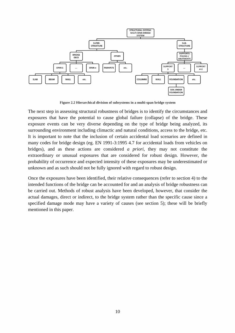
The primary function of most bridge structures is to maintain a safe and continuous flow of traffic in whatever form; i.e. pedestrian, cycle, vehicular, train or ship. This function is maintained via the combined interactions of its structural components which comprise the sub-systems of the bridge system. Localized failure to one of more components will create direct consequence to the relative structural elements which may lead to indirect consequence on a more global level (such as progressive collapse). Therefore it is important to understand the relations between sub-systems and their significance on the system as a whole. Figure 2.2 shows a general example for the hierarchical division of subsystems for an arbitrary multi-span concrete frame bridge.

10

Figure 2.2 Hierarchical division of subsystems in a multi-span bridge system

The next step in assessing structural robustness of bridges is to identify the circumstances and exposures that have the potential to cause global failure (collapse) of the bridge. These exposure events can be very diverse depending on the type of bridge being analyzed, its surrounding environment including climactic and natural conditions, access to the bridge, etc. It is important to note that the inclusion of certain accidental load scenarios are defined in many codes for bridge design (eg. EN 1991-3:1995 4.7 for accidental loads from vehicles on bridges), and as these actions are considered a priori, they may not constitute the extraordinary or unusual exposures that are considered for robust design. However, the probability of occurrence and expected intensity of these exposures may be underestimated or unknown and as such should not be fully ignored with regard to robust design.

Once the exposures have been identified, their relative consequences (refer to section 4) to the intended functions of the bridge can be accounted for and an analysis of bridge robustness can be carried out. Methods of robust analysis have been developed, however, that consider the actual damages, direct or indirect, to the bridge system rather than the specific cause since a specified damage mode may have a variety of causes (see section 5); these will be briefly mentioned in this paper.

11

3. Circumstances for failure

3.1 General overview The growth of structural forensic engineering as an active professional field in the modern day engineering world leaves much to be said about the increase of structural failures today. In an ideal world, the need for such investigation would become unnecessary and structures would perform as intended. However, “…demands of rapid economic development, increased design sophistication, more and more daring construction technology, and accelerated project delivery increase the number of [structural] failures throughout the world…” (Ratay 2007) In light of this, it has become even more paramount not to take short-cuts and neglect issues regarding structural robustness during the design and execution of structures. The first step in trying to understand problems with robustness and collapse of bridges is to identify the relative circumstances for which failure may occur.

Investigations of actual bridge failures have been collected and summarized by Åkesson (2008), Sheer (2000) and Wardhana et al. (2003) to name a few. It is important to build upon the results of investigations such as these as a basis for research of robustness of bridges. Clearly the bridges were not adequately robust and the analysis of their failure helps to identify recurring collapse-promoting features. Most bridge failures occur during the construction phase of the structural systems lifespan, such as failure of scaffolding during erection (Galambos 2008). However, the focus of this paper will be on bridge failures that occur during the working life of a bridge; i.e. while it is in operation.

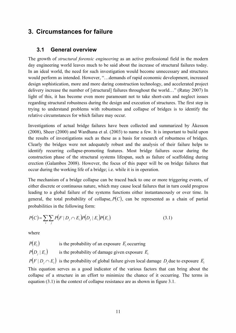
The mechanism of a bridge collapse can be traced back to one or more triggering events, of either discrete or continuous nature, which may cause local failures that in turn could progress leading to a global failure of the systems functions either instantaneously or over time. In general, the total probability of collapse, ( )CP , can be represented as a chain of partial probabilities in the following form:

( ) ( ) ( ) ( )∑∑ ∩=i j

iijij EPEDPEDFPCP || (3.1)

where

( )iEP is the probability of an exposure iE occurring

( )ij EDP | is the probability of damage given exposure iE

( )ij EDFP ∩| is the probability of global failure given local damage jD due to exposure iE

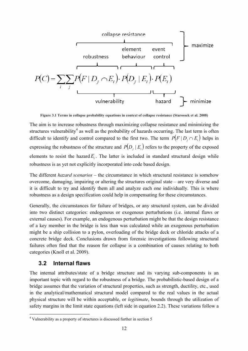
This equation serves as a good indicator of the various factors that can bring about the collapse of a structure in an effort to minimize the chance of it occurring. The terms in equation (3.1) in the context of collapse resistance are as shown in figure 3.1.

12

Figure 3.1 Terms in collapse probability equations in context of collapse resistance (Starossek et al. 2008)

The aim is to increase robustness through maximizing collapse resistance and minimizing the structures vulnerability4 as well as the probability of hazards occurring. The last term is often difficult to identify and control compared to the first two. The term ( )ij EDFP ∩| helps in

expressing the robustness of the structure and ( )ij EDP | refers to the property of the exposed

elements to resist the hazard iE . The latter is included in standard structural design while robustness is as yet not explicitly incorporated into code based design.

The different hazard scenarios – the circumstance in which structural resistance is somehow overcome, damaging, impairing or altering the structures original state – are very diverse and it is difficult to try and identify them all and analyze each one individually. This is where robustness as a design specification could help in compensating for these circumstances.

Generally, the circumstances for failure of bridges, or any structural system, can be divided into two distinct categories: endogenous or exogenous perturbations (i.e. internal flaws or external causes). For example, an endogenous perturbation might be that the design resistance of a key member in the bridge is less than was calculated while an exogenous perturbation might be a ship collision to a pylon, overloading of the bridge deck or chloride attacks of a concrete bridge deck. Conclusions drawn from forensic investigations following structural failures often find that the reason for collapse is a combination of causes relating to both categories (Knoll et al. 2009).

3.2 Internal flaws The internal attributes/state of a bridge structure and its varying sub-components is an important topic with regard to the robustness of a bridge. The probabilistic-based design of a bridge assumes that the variation of structural properties, such as strength, ductility, etc., used in the analytical/mathematical structural model compared to the real values in the actual physical structure will be within acceptable, or legitimate, bounds through the utilization of safety margins in the limit state equations (left side in equation 2.2). These variations follow a 4 Vulnerability as a property of structures is discussed further in section 5

13

statistical distribution for random data, usually Gaussian, developed through past research. In addition to the use of safety margins, testing, inspection and quality control procedures are performed in an effort to eliminate any extreme variations. However, the involvement of humans in a process of production or execution of structural systems/subsystems of which these structural properties adhere indicate that these variations are subject to the consequences of human error; a phenomena for which no probability law currently exists (Knoll et al. 2009). Human error can occur during all stages of the bridges development and lifespan:

• Error during design - inadequate resistance, ductility, etc. • Error during construction - poorly chosen building procedures, poor communication,

etc. • Error during operation - inadequate inspection, maintenance, reparations, etc.

All three types of human errors listed above may result in internal flaws in the bridge structure.

Gross human error is therefore a significant element of the internal flaw hazard scenario. One way to try and decrease its impact is through quality control during the design and construction processes; i.e. a filtering process which tries to eliminate the larger variations in structural properties during design (by checking calculations, drawings, etc.), construction (supervision on site) and operation (periodic maintenance and inspection, etc.). There is no way, however, to completely eliminate the possibility of gross human errors occurring. The only way to compensate for its consequences is with adequate structural robustness.

3.3 External exposures A bridge structure is subject to a wide variety of exogenous perturbations throughout its service life continuously testing the capacity of the structure. This section will focus on exposures not included in normal design of bridges. However, in some cases the effect of anticipated exposures to an unanticipated degree may result in the collapse of a bridge. Furthermore, flaws in the design or construction of the structure may result in failure even in the absence of extraordinary or unanticipated circumstances. Research of collapsed bridges helps to identify certain recurring circumstances of collapse which can then aid for future design in which these circumstances are taken into account.

If a sufficient amount of data exists for an external hazard scenario it can be included in the design of the bridge through analytical or testing procedures; i.e. either mathematical or physical modeling. This should be done with regard to the consequences of specific exposures to the system as a whole and not only via usual component based design. A localized component of a bridge may be designed such that it is sufficiently resilient to extraordinary hazard scenarios, however, this is sometimes not cost efficient or pragmatically plausible in all cases (Knoll et al. 2009). This issue will be touched upon in section 5.

14

It is important to try and get a deeper understanding of common failure scenarios when analyzing the robustness of a bridge structure. The following are some key external exposures that could result in structural failure of bridges:

Overloading ‐ This may include anticipated loading of a flawed structure

Accidents ‐ eg. collisions, fires, etc.

Fatigue/deterioration ‐ Although the structure is designed to withstand the individual exposures and

events, the cumulative effect of various exposures, such as chemical attacks, dynamic loading, etc, could cause the structure to weaken and then in time fail.

Malevolence (purposeful destruction) Natural events

‐ eg. floods, extreme weather, etc.

The cause of the damage could also be any combination of these. It is therefore hard to identify explicit design criteria which take all of these into account; however, certain methods have been developed to help incorporate robustness into the design of a structure.

While the internal flaws discussed in the previous section creates uncertainties in the resistance of the structure (left side in eq. (2.2)), the variety and randomness of external perturbations effecting the structure also introduce uncertainty into its design (right side in eq. (2.2)). These safety margins are chosen with the aid of statistical and probabilistic analysis of empirical data in order to account for deviations between mathematical/analytical models and the real structure. However, forensic investigation following the collapse of structures often recognizes that collapse was not the result of poorly chosen safety margins or factors during design, but was caused by something altogether unanticipated (Knoll et al. 2009).

3.4 Hierarchy of failure modes The previous sections give a general overview of the different types of extraordinary or unanticipated exposures that may bring about the collapse of a bridge system. These exposures may, however, cause bridges to fail in different ways in which different failure modes must be considered. Each mode of failure gives a description of the course of events leading up to collapse including the consequences to the bridge system (Knoll et al. 2009). It is possible to identify these different scenarios and rank the varying degrees of failure/damage to the bridge system using probabilistic methods. From equation (3.1) it is noted that for each initiating event Ei there are varying local damages Dj that may be expected to occur. The degree of sensitivity of the bridge system to global failure from the local damages will differ such that a hierarchy of failure modes may be extracted; i.e. the consequences of each failure mode must be considered (see section 4). A robust bridge structure is one that is more insensitive to global failure given the worst-case failure mode; i.e. the bridge system develops less catastrophic failure modes.

15

In order to ascertain a hierarchy of different failure modes for a bridge structure, actual conditions must be considered without the use of load or resistance factors. This is difficult to model exactly and especially a-priori (i.e. prior to completion of structure) since the degree of deviation between the designed (idealized) and built structure cannot be evaluated until after its completion; and even then it cannot be determined exactly – the bridge cannot be tested directly for robustness. The use of stochastic (probabilistic) design methods with regards to robustness evaluation is then very helpful in considering these deviations and obtaining a hierarchy of failure modes.

Once the relevant hazard scenarios for a bridge structure have been identified and all failure modes considered, the mechanism of collapse can be determined. The system’s response to a specific exposure can be traced. It is analogous to a row of dominoes toppling over one after the other; damage to one component propagates to another and ultimately leading to collapse.

16

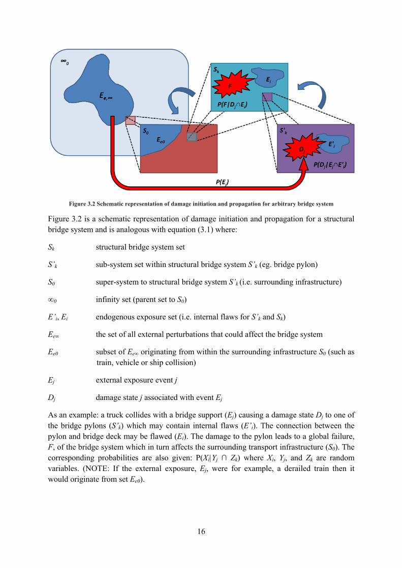
Figure 3.2 Schematic representation of damage initiation and propagation for arbitrary bridge system

Figure 3.2 is a schematic representation of damage initiation and propagation for a structural bridge system and is analogous with equation (3.1) where:

Sk structural bridge system set

S’k sub-system set within structural bridge system S’k (eg. bridge pylon)

S0 super-system to structural bridge system S’k (i.e. surrounding infrastructure)

∞0 infinity set (parent set to S0)

E’i, Ei endogenous exposure set (i.e. internal flaws for S’k and Sk)

Ee∞ the set of all external perturbations that could affect the bridge system

Ee0 subset of Ee∞ originating from within the surrounding infrastructure S0 (such as train, vehicle or ship collision)

Ej external exposure event j

Dj damage state j associated with event Ej

As an example: a truck collides with a bridge support (Ej) causing a damage state Dj to one of the bridge pylons (S’k) which may contain internal flaws (E’i). The connection between the pylon and bridge deck may be flawed (Ei). The damage to the pylon leads to a global failure, F, of the bridge system which in turn affects the surrounding transport infrastructure (S0). The corresponding probabilities are also given: P(Xi|Yj ∩ Zk) where Xi, Yj, and Zk are random variables. (NOTE: If the external exposure, Ej, were for example, a derailed train then it would originate from set Ee0).

17

4. Consequences of failure

4.1 Consequences to structural system The key aspect of a robust structure is its ability to maintain an acceptable degree of functionality after a damaging event occurs or, alternatively, partially lose functionality for a limited period of time. For a bridge, the main function is to maintain traffic flow while some damage may be acceptable in that it is localized or to a degree in which its function is only partially affected or limited in time. Thus an acceptable degree of global consequence (i.e. consequences to the entire system) may be specified on a case by case basis. In some extreme cases it may be acceptable that a bridge loose total functionality while user safety can be ensured. Eurocode 0 proposes so called consequences classes considering the failure or malfunction of a structure (EN 1990:2002):

CC1 o “High consequence for loss of human life, or economic, social or

environmental consequences very great” CC2

o “Medium consequences for loss of human life, economic, social or environmental consequences considerable”

CC3 o “Low consequences for loss of human life, and economic, social or

environmental consequences small or negligible”

These consequences classes correspond to different reliability classes which prescribe acceptable limits for structural failure probabilities as a basis of design for structures in general. A reliability index, β, is defined which is determined as the inverse standardized normal distribution of the probability of failure, Pf. (EN 1990:2002)

( )yearfn Pn 1.1 ⋅Φ−= −β (4.1)

n reference period in years

Pf.1year probability of structural failure for a reference period of 1 year

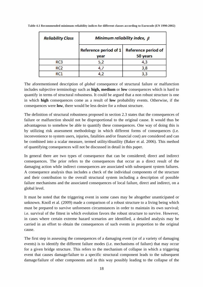
Table 4.1 shows the target reliabilities indices for reference periods of 1 and 50 years according to Eurocode for ultimate limit state design (i.e. design concerning safety of people and/or structure). The reliability classes RC3, RC2 and RC1 correspond to the consequence classes CC3, CC2 and CC1.

18

Table 4.1 Recommended minimum reliability indices for different classes according to Eurocode (EN 1990:2002)

The aforementioned description of global consequence of structural failure or malfunction includes subjective terminology such as high, medium or low consequences which is hard to quantify in terms of structural robustness. It could be argued that a non robust structure is one in which high consequences come as a result of low probability events. Otherwise, if the consequences were low, there would be less desire for a robust structure.

The definition of structural robustness proposed in section 2.3 states that the consequences of failure or malfunction should not be disproportional to the original cause. It would thus be advantageous to somehow be able to quantify these consequences. One way of doing this is by utilizing risk assessment methodology in which different forms of consequences (i.e. inconvenience to system users, injuries, fatalities and/or financial cost) are considered and can be combined into a scalar measure, termed utility/disutility (Baker et al. 2006). This method of quantifying consequences will not be discussed in detail in this paper.

In general there are two types of consequence that can be considered; direct and indirect consequences. The prior refers to the consequences that occur as a direct result of the damaging action while indirect consequences are associated with subsequent system failures. A consequence analysis thus includes a check of the individual components of the structure and their contribution to the overall structural system including a description of possible failure mechanisms and the associated consequences of local failure, direct and indirect, on a global level.

It must be noted that the triggering event in some cases may be altogether unanticipated or unknown. Knoll et al. (2009) made a comparison of a robust structure to a living being which must be prepared to survive unforeseen circumstances in order to maintain its own survival; i.e. survival of the fittest in which evolution favors the robust structure to survive. However, in cases where certain extreme hazard scenarios are identified, a detailed analysis may be carried in an effort to obtain the consequences of such events in proportion to the original cause.

The first step in assessing the consequences of a damaging event (or of a variety of damaging events) is to identify the different failure modes (i.e. mechanisms of failure) that may occur for a given bridge structure. This refers to the mechanism of collapse in which a triggering event that causes damage/failure to a specific structural component leads to the subsequent damage/failure of other components and in this way possibly leading to the collapse of the

19

entire structure. The direct and indirect consequence of each propagating action can then be analyzed separately to try and identify key collapse-promoting features and extract possible counter-measures (Starossek 2009). A typology and classification of progressive collapse of structures has been researched by Starossek (2009) and will not be specifically mentioned in this paper.

20

4.2 Consequences to super-system The super system for a bridge structure is the surrounding infrastructure including transport networks such as road, railway, marine and pedestrian networks. Their reliance on the bridge structure itself is relatively localized but the failure of the latter may have varying degrees of consequences to the infrastructure network. This is heavily dependent on the layout (topology) of the network and location of the bridge within that network

The function of the super system is not that different from the bridge system itself in that it should maintain traffic flow, however it can do this via various routes. Furthermore, the infrastructure network is in effect a living entity in that it constantly changes with time; i.e. the distribution of traffic flow constantly changes, user demand may vary and the geometric layout may even change – eg. new arteries are created or old ones rebuilt and temporarily closed.

A topology of the infrastructure network can be created and its functionality assessed using methods of traffic design; these methods will not be discussed in this paper. The impact of a bridge failing on the infrastructure network can then be ascertained by comparing the intact and impaired infrastructure system. The consequences of bridge failure within an infrastructure system are varied and the super-system’s robustness may be evaluated using similar methods related to structural robustness

21

5. Strategies & methods of Robustness

5.1 Introduction There have been some methods and strategies developed towards quantifying robustness or similar attributes (vulnerability, collapse resistance, etc.) and achieving greater robustness in structures recently but they remain scattered and thus far no general approach has been universally accepted regarding design for robustness. For the most part, recent developments of methods and strategies for robust design have focused on structural building systems while to a lesser degree for structural bridge systems (Starossek 2009). This is probably due largely to the significance of recent building collapses such as the WTC in New York, 2001, and the Oklahoma City bombing in 1995.

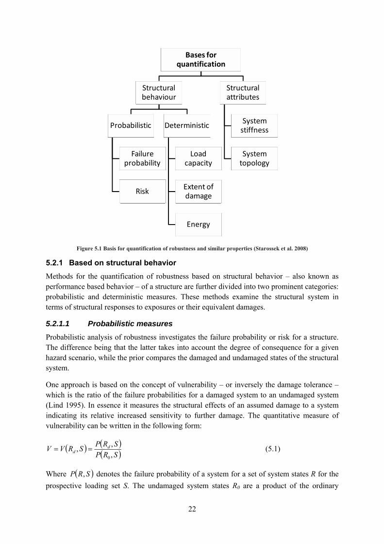
5.2 Methods for quantification of Robustness Currently there exist various methods and approaches for the quantification of robustness or similar structural properties (eg. vulnerability) which have been developed in the past few years including probabilistic measures of vulnerability (Lind 1995), detailed risk-consequence analysis (Maes et. al. 2006) and probabilistic risk assessment (Baker et al. 2006) to name a few (see also Agarwal et al. 2003, Smith 2006 and Wisniewski et al. 2007). Starossek et al. (2008) have comprised these approaches and distinguished them into two prominent categories: measures based on (1) structural behavior (or performance) and (2) structural attributes of systems. A basis for robustness quantification was developed and further sub-categorization determined as shown in Figure 5.1.

22

Figure 5.1 Basis for quantification of robustness and similar properties (Starossek et al. 2008)

5.2.1 Based on structural behavior Methods for the quantification of robustness based on structural behavior – also known as performance based behavior – of a structure are further divided into two prominent categories: probabilistic and deterministic measures. These methods examine the structural system in terms of structural responses to exposures or their equivalent damages.

5.2.1.1 Probabilistic measures Probabilistic analysis of robustness investigates the failure probability or risk for a structure. The difference being that the latter takes into account the degree of consequence for a given hazard scenario, while the prior compares the damaged and undamaged states of the structural system.

One approach is based on the concept of vulnerability – or inversely the damage tolerance – which is the ratio of the failure probabilities for a damaged system to an undamaged system (Lind 1995). In essence it measures the structural effects of an assumed damage to a system indicating its relative increased sensitivity to further damage. The quantitative measure of vulnerability can be written in the following form:

( ) ( )( )SRP

SRPSRVV dd ,

,,0

== (5.1)

Where ( )SRP , denotes the failure probability of a system for a set of system states R for the prospective loading set S. The undamaged system states R0 are a product of the ordinary

Bases for quantification

Structural behaviour

Probabilistic

Failure probability

Risk

Deterministic

Load capacity

Extent of damage

Energy

Structural attributes

System stiffness

System topology

23

loading set S0 which affect the system without damaging it. The damage spectrum for which vulnerability is to be considered is given by Rd.

Maes et al. (2006) determined a similar approach which compares system failure probabilities of an undamaged system state, 0sP , and a damaged state, siP (i.e. the system failure probability for an undamaged system versus the system failure probability for a system with one impaired member/element i):

si

si P

PR 0min= (5.2)

The aforementioned probabilistic methods, however, fail to take into account the consequences of system failure. Maes et al. (2006) also proposed a more detailed risk-consequence analysis of a structural system which compares the hazard intensity (X) with a cost associated with the consequences of failure (CF). In this way a function of failure consequence versus hazard intensity can be plotted and the probability of exceedance obtained by integrating over the probability density function of the hazard itself. A measure of robustness is also proposed.

A probabilistic risk assessment based approach has been introduced by Baker et al. (2006) which defines robustness as the proportionality of consequences of structural damage to the cause. A so called robustness index is formulated as a quantification of robustness. This approach will be discussed in more detail in section 5.2.3.

5.2.1.2 Deterministic measures The deterministic approaches towards quantification of robustness in some cases also compare the original and damaged state of a system. However, they differ from probabilistic methods in that they do not incorporate failure probabilities or require statistical input data. For example, Maes et al. (2006) determined a measure based on the so-called reserve strength ratio (RSR) which compares the system strength in a damaged and undamaged state (denoted by i and 0 respectively):

0

minRSRRSRR i

i= (5.3)

A similar measure has been determined by Wisniewski et al. (2006). Other approaches formulated include Starossek (2009) which analyzes the extent of damage progression of a system and Smith (2006), an energy based approach comparing progressive collapse of a structure with the fast fracture theory of metals.

In all aforementioned cases, the deterministic robustness approaches do not take into account the consequences of failure which, as was stated in previous sections, have been deemed pertinent to the assessment of robustness of structures.

5.2.2 The meincludinmeasureactive sstructur

minRi

=

Agarwa3D framinherentstructur

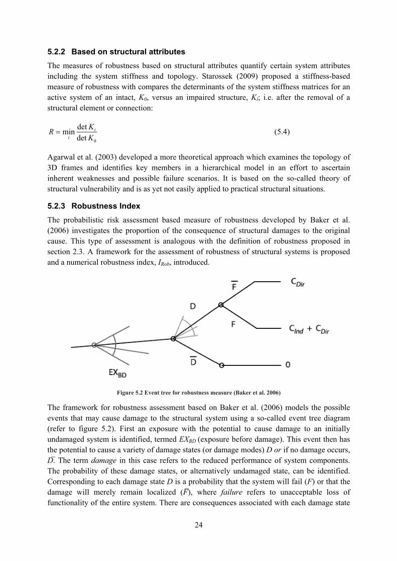
5.2.3 The pro(2006) cause. Tsection and a nu

The framevents t(refer toundamathe poteD̅. The The proCorrespdamagefunction

Based on easures of rng the syste of robustnsystem of aral element o

0detdetn

KKi

al et al. (200mes and idt weakness

ral vulnerab

Robustneobabilistic rinvestigatesThis type o2.3. A fram

umerical rob

mework forthat may cao figure 5.2aged systemential to cau

term damaobability of ponding to ee will merenality of the

structurarobustness btem stiffnesness with coan intact, Kor connectio

03) developdentifies kees and posility and is

ess Index risk assessms the propoof assessmemework for bustness ind

Figure 5.2

r robustnesause damag2). First an

m is identifieuse a varietyage in this cf these dameach damagely remain e entire syst

al attributebased on stss and topoompares the

K0, versus anon:

ped a more ty members

ssible failuras yet not e

ment basedortion of theent is analo

the assessmdex, IRob, in

Event tree for

s assessmenge to the strn exposure ed, termed Ey of damagecase refers

mage states, ge state D is

localized tem. There

24

es tructural attology. Staroe determinann impaired

theoretical as in a hierare scenarioseasily applie

d measure oe consequen

ogous with ment of rob

ntroduced.

r robustness m

nt based onructural sys

with the pEXBD (expo

e states (or dto the reduor alternati

s a probabil(F̅), whereare consequ

tributes quaossek (200nts of the systructure, K

approach warchical mos. It is baseed to practic

of robustnence of structhe definiti

bustness of

easure (Baker

n Baker et atem using a

potential to osure beforedamage mouced performively undamity that the

e failure reuences asso

antify certai9) proposeystem stiffnKi; i.e. afte

(5.4

which examiodel in an ed on the cal structura

ess developctural damaion of robustructural s

et al. 2006)

al. (2006) ma so-called cause dam

e damage). Tdes) D or ifmance of s

maged statesystem wil

efers to unociated with

in system ad a stiffneness matriceer the remo

)

ines the topeffort to a

so-called thal situations

ed by Bakages to the ustness propsystems is p

models the event tree

mage to an This event f no damageystem com

e, can be idl fail (F) or

nacceptable h each dama

attributes ss-based es for an

oval of a

ology of ascertain heory of .

ker et al. original

posed in proposed

possible diagram initially then has e occurs,

mponents. dentified. r that the

loss of age state

25

which are either classified as direct, CDir, or indirect, CInd, consequences (refer to section 4.1). Thus in the case where failure of the system does not occur (F̅), there are only direct consequences to the system. While in the case where failure does occur (F), there is an additional indirect consequence to the system due to damage state D. And of course if no damage occurs to the system (D̅) for an exposure event EXBD then there are no consequences, C = 0.

While current design codes incorporate a check of possible damage scenarios and resulting consequences, such that their proportionality can be checked, the robustness measure proposed by Baker et al. (2006) requires that the probability of the originating exposures be included for the quantification of robustness.

The variety of possible exposure events, EXBD, damage modes, D, and associated failure scenarios, F or F̅, must be considered in order to achieve a concise measure of risk to the system and thus be able to allocate resources for risk reduction. The risk of an exposure event is equal to the consequence associated with that event multiplied by the probability of occurrence. In this way the total direct and indirect risks for a set of event exposures (i.e. hazard scenario) and possible damage states can be calculated according to the following formulas (Champris 2008):

( ) ( ) ( )∑∑ ⋅⋅=i j

iBDiBDjjDirDir EXPEXDPDCR ..| (5.5a)

( ) ( ) ( ) ( )∑∑ ⋅⋅⋅=i j

iBDiBDjjIndInd EXPEXDPDFPFCR ..|| (5.5b)

where the probability of failure for a given damage is assumed conditionally independent of the exposure causing it.

An index of robustness is formulated which is defined as the ratio of direct risk to the structural system to the total risk:

IndDir

Dir

total

DirRob RR

RRRI

+== (5.6)

The robustness index from the above equation can then only give values ranging from zero to one. In which a completely robust structure is defined for the case in which there are no indirect risks (IRob = 1). While a completely non robust structure would have a robustness index of IRob = 0 (Baker et al. 2006).

The aforementioned assessment of robustness was then further developed by incorporating decision analysis theory. This is more representative of actual engineered systems which are subject to actions taken by those responsible for its design, maintenance, inspection, etc. The event tree from figure 5.2 can then be broadened to include system choices and possible post-damage exposures. The details of this framework of robustness assessment and corresponding robustness index will not be discussed here (read Baker et al. 2006).

26

5.3 Strategies towards greater Robustness of Bridges There currently exist various strategies to help prevent disproportionate failure of structures which differ in their aptness in application directly for bridge structures. In comparison to building structures, bridges are primarily horizontally aligned structures with one main axis of extension (Starossek 2009). Their failure mechanism differs from that of buildings and while buildings exhibit some inherent redundancies a bridge system is usually composed of elements all of which are intended for structural usage; i.e. their combined structural resistances comprise the total resistance of the structural system in its entirety.

Current strategies towards increasing the robustness of bridges structures can be divided into the following categories (Starossek 2009):

‐ Prevent local failure of critical elements; first line of defense Control local resistance Protective measures

‐ Assume local failure; second line of defense Alternative load paths Isolation by segmentation

‐ Prescriptive design rules

These different methods may vary in their suitability for different bridge structures. This has much to do with the robustness requirements designated for the bridge structure in question. In some cases there may be an acceptable degree of collapse while in others the maintained structural integrity of the bridge is paramount. These robustness requirements must therefore be prescribed in the design specifications for the bridge with adequate justification.

5.3.1 Prevent local failure of critical elements: first line of defense One direct approach to help prevent disproportionate collapse of bridges structures is to prevent the local failure of critical elements; also known as the first line of defense strategy. A critical element is a structural component that produces an unacceptably large failure progression in the structural system (i.e. degree of progressive collapse). Critical elements may be identified through intuitive or analytical procedures; for example, by checking extent of collapse progression for a removed structural component. To help increase the robustness of the bridge, the design of the bridge must include measures that hinder the failure of these elements specifically. This can be done in two different ways: (1) provide adequate local resistance to prevent failure or (2) introduce protective or sacrificial devices. This method is also known as the first line of defense.

Increasing the local resistance of a critical element within the structural bridge system is quite straightforward and can be prescribed directly in the design requirements. In cases where increased resistance is uneconomical or not possible, non-structural protective measures can be used. These measures could include physical barriers, surveillance systems, etc. However, both of these strategies require that the extraordinary exposure events be identified in which case unanticipated hazard scenarios may be overlooked; i.e. the level of safety desired may not be as high as required in light of unknown future actions (Starossek 2009).

27

The effectiveness of this method varies from bridge to bridge. In some cases the first line of defense strategy may be ineffective (or uneconomical) and other measures to increase robustness need to be considered; for example, if the bridge is highly exposed or the number of critical elements is high.

5.3.2 Assume local failure: Second line of defense If prevention of local failure of critical elements of a bridge structure cannot be achieved – which in actuality can never be absolutely achieved – the only compromise is to account for localized failure and implement measures to help minimize the overall consequences such that structural robustness is increased. This method of increasing robustness is favorable for highly exposed or very significant bridges, where the consequences of collapse are great (Starossek 2006). This would include long span bridges where user safety is imperative (of greater consequence) or where the transport network is heavily reliant on the bridge; for example, the Öresund bridge between Sweden and Denmark.

This method of assuming local failure can be advantages in that it is independent of the hazard scenario causing the damage. It analyzes the consequence of assumed local failure of critical elements. The acceptable extent of local failure should be prescribed in the design objectives.

5.3.2.1 Multiple load paths or redundancy In a situation where the structural integrity of a bridge structure is heavily reliant on a single critical component, the assumable failure of such a component may be hard to overcome for the residual structural capacity of the remaining structure. It is therefore helpful to “share” the load via utilizing several different load paths and thereby creating some redundancy in the structural system. By this it is meant that various load paths are utilized initially in which the structural forces are channeled through all of them (Knoll et al. 2009). Thus if one path were to fail or malfunction, the rest may be able to continue resisting the loads; i.e. residual capacity remains greater than residual loading after a damaging event.

The ability of a bridge structure to mobilize multiple load paths relies heavily on the bridge systems’ sub-components collective structural behavior to external perturbations. In the case where a critical element is removed, the remaining structural components must have enough residual capacity to resist the residual loading demands. It is also important to analyze the mechanism of failure for the impaired structure to ensure that the transference of loading from the knocked-out member to the remaining structure is achievable. In cases where an acceptable degree of damage progression is prescribed, it is important for the remaining system to adopt the structural functions of all failed elements and maintain overall structural stability (at least for a limited period of time to ensure user safety or implement reparative measures).

The existence of multiple loading paths in an engineered structural system shall be referred to as redundancy (Starossek 2009). This could include the modification of a structural system such that a number of elements share the loading or the strengthening of a member for the purpose of creating a resilient alternative load path in case of the failure of an adjoining

28

member. For example, if the support for a bridge system were to fail, the bridge deck could be designed with the strength required to resist the residual loading demand for the impaired bridge system.

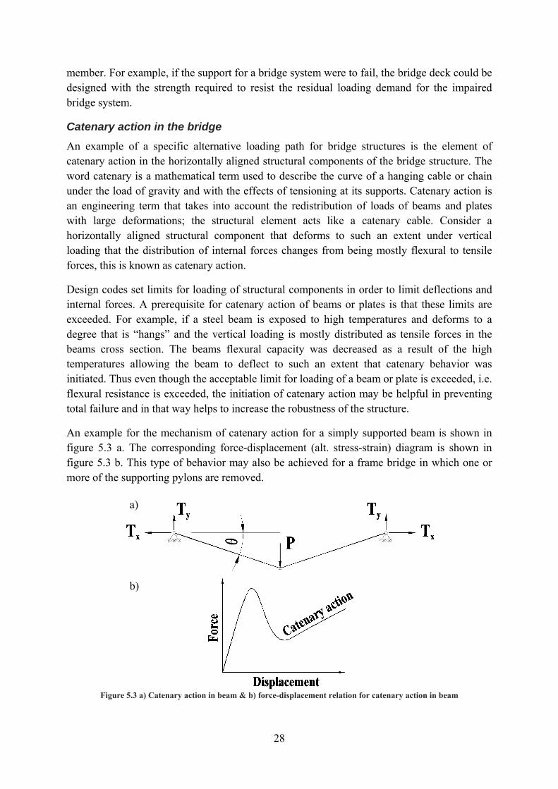
Catenary action in the bridge An example of a specific alternative loading path for bridge structures is the element of catenary action in the horizontally aligned structural components of the bridge structure. The word catenary is a mathematical term used to describe the curve of a hanging cable or chain under the load of gravity and with the effects of tensioning at its supports. Catenary action is an engineering term that takes into account the redistribution of loads of beams and plates with large deformations; the structural element acts like a catenary cable. Consider a horizontally aligned structural component that deforms to such an extent under vertical loading that the distribution of internal forces changes from being mostly flexural to tensile forces, this is known as catenary action.

Design codes set limits for loading of structural components in order to limit deflections and internal forces. A prerequisite for catenary action of beams or plates is that these limits are exceeded. For example, if a steel beam is exposed to high temperatures and deforms to a degree that is “hangs” and the vertical loading is mostly distributed as tensile forces in the beams cross section. The beams flexural capacity was decreased as a result of the high temperatures allowing the beam to deflect to such an extent that catenary behavior was initiated. Thus even though the acceptable limit for loading of a beam or plate is exceeded, i.e. flexural resistance is exceeded, the initiation of catenary action may be helpful in preventing total failure and in that way helps to increase the robustness of the structure.

An example for the mechanism of catenary action for a simply supported beam is shown in figure 5.3 a. The corresponding force-displacement (alt. stress-strain) diagram is shown in figure 5.3 b. This type of behavior may also be achieved for a frame bridge in which one or more of the supporting pylons are removed.

Figure 5.3 a) Catenary action in beam & b) force-displacement relation for catenary action in beam

a)

b)

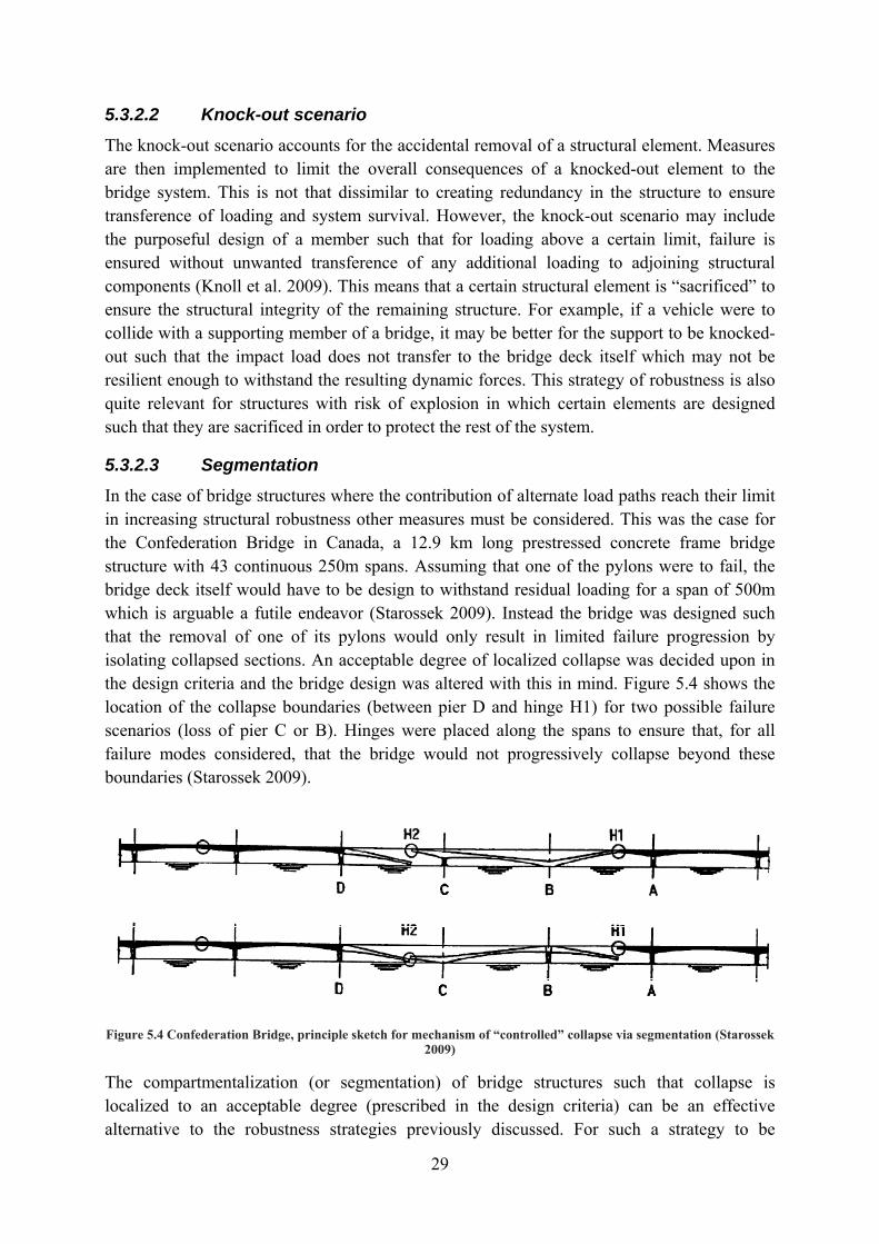
29

5.3.2.2 Knock-out scenario The knock-out scenario accounts for the accidental removal of a structural element. Measures are then implemented to limit the overall consequences of a knocked-out element to the bridge system. This is not that dissimilar to creating redundancy in the structure to ensure transference of loading and system survival. However, the knock-out scenario may include the purposeful design of a member such that for loading above a certain limit, failure is ensured without unwanted transference of any additional loading to adjoining structural components (Knoll et al. 2009). This means that a certain structural element is “sacrificed” to ensure the structural integrity of the remaining structure. For example, if a vehicle were to collide with a supporting member of a bridge, it may be better for the support to be knocked-out such that the impact load does not transfer to the bridge deck itself which may not be resilient enough to withstand the resulting dynamic forces. This strategy of robustness is also quite relevant for structures with risk of explosion in which certain elements are designed such that they are sacrificed in order to protect the rest of the system.

5.3.2.3 Segmentation In the case of bridge structures where the contribution of alternate load paths reach their limit in increasing structural robustness other measures must be considered. This was the case for the Confederation Bridge in Canada, a 12.9 km long prestressed concrete frame bridge structure with 43 continuous 250m spans. Assuming that one of the pylons were to fail, the bridge deck itself would have to be design to withstand residual loading for a span of 500m which is arguable a futile endeavor (Starossek 2009). Instead the bridge was designed such that the removal of one of its pylons would only result in limited failure progression by isolating collapsed sections. An acceptable degree of localized collapse was decided upon in the design criteria and the bridge design was altered with this in mind. Figure 5.4 shows the location of the collapse boundaries (between pier D and hinge H1) for two possible failure scenarios (loss of pier C or B). Hinges were placed along the spans to ensure that, for all failure modes considered, that the bridge would not progressively collapse beyond these boundaries (Starossek 2009).

Figure 5.4 Confederation Bridge, principle sketch for mechanism of “controlled” collapse via segmentation (Starossek 2009)

The compartmentalization (or segmentation) of bridge structures such that collapse is localized to an acceptable degree (prescribed in the design criteria) can be an effective alternative to the robustness strategies previously discussed. For such a strategy to be

30

implemented, the remaining structure must be closely analyzed for loads resulting from the localized collapse. It must be ensured that the collapse remains localized and does not propagate any further. The mechanism of relevant failure modes must be investigated and the resulting mechanisms of collapse analyzed to ensure segmentation is effective (Starossek 2009).

This method of ensuring structural robustness of bridges is analogous to controlled demolition in that the collapse progression is controlled and localized to only a portion of the structure. The suitability of segmentation versus multiple load paths or first line of defense depends on the bridge structure being analyzed. It is therefore important to prescribe design criteria which include robustness requirement of the structure; i.e. is limited collapse acceptable and to what degree, etc.

5.3.3 Prescriptive design rules Thus far the previous strategies of increasing robustness of bridge structures involve direct approaches which require complex analysis of the structural response of a bridge system to hazard scenarios. These procedures are quite tedious and time consuming and may require much computational power. Utilizing this type of analysis for smaller bridge structure may be asking too much. The use of prescriptive design rule which are included in structural codes (eg. Eurocode 0, refer to section 2.4.2) may instead be adopted. The most common rules are the following (Starossek 2006):

• Tying structural elements together • Enabling catenary action • Providing ductility

These rules help to ensure overall structural integrity of bridge systems but should be applied with discretion and not be considered the end-all requirement to ensure robustness. Since empirical knowledge of collapse progression of bridges is limited (i.e. due to the rarity of the event) there is still much to be learned with regard to robustness promoting features and their effectiveness. Every bridge should therefore be carefully examined in an effort to extrapolate which method of robust design should be implemented and whether detailed analysis is required or if prescriptive design requirements are adequate.

31

6. Robustness considerations of Sjölundaviadukten Bridge

6.1 Introduction The previous sections of the report gave an overview of structural robustness as a property of bridge structures including a discussion of its application in the design of bridges. Various methods of quantifying robustness have been mentioned as well as strategies aimed at increasing overall structural robustness for bridge structures. Thus far the concept of structural robustness has been examined in a relatively wide context without going into much detail with regard to its application for specific bridge structures. The best way in achieving a better understanding of structural robustness as a property of bridge structures is to conduct a case study thereby incorporating the points of discussion from the previous section of this report.

This section of the report considers a post-tensioned reinforced concrete road bridge, the Sjölundaviadadukt Bridge in Malmö, Sweden, with regard to its structural robustness. The purpose of this examination is to attempt at a framework for the analysis of structural robustness for an arbitrary bridge structure. The focus of this study is of the methodology for structural robustness considerations rather than of the specific analytical procedures.

32

6.2 Background The Sjölundaviadukt Bridge is a post-tensioned reinforced concrete road bridge with 5 spans for a total length of around 190m. The bridge is currently under construction and is being built to replace an older bridge which can be seen on figure 6.1; it is expected to be completed in the spring of 2010. The original bridge was first completed in 1931 and later in 1968. The original design was deemed inadequate to support the amount and size of heavy traffic it is currently exposed to and there was a risk that it might fail as a result of this [4].

Figure 6.1 Aerial photo of old Sjölundaviadukt Bridge in Malmö [5]

The bridge deck consists of a double lane road [K 4.975] including adjacent walkways and cycle lanes [G 1.625 C 2.0] on either side for a total deck breadth of around 20m. The traffic running under the bridge consists of 16 railroad tracks for goods and commuter train traffic as well as a 4 lane road highway. The substructure consists of 4 pylons and 2 abutments made from reinforced concrete. Traffic information for the surrounding infrastructure elements including road and railway arteries is given in section 6.3.1.

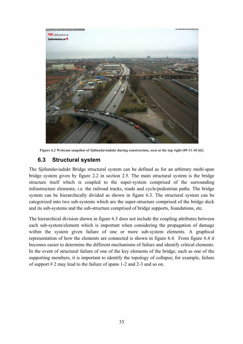
33

Figure 6.2 Webcam snapshot of Sjölundaviadukt during construction, seen at the top right (09-11-10 [6])

6.3 Structural system The Sjölundaviadukt Bridge structural system can be defined as for an arbitrary multi-span bridge system given by figure 2.2 in section 2.5. The main structural system is the bridge structure itself which is coupled to the super-system comprised of the surrounding infrastructure elements; i.e. the railroad tracks, roads and cycle/pedestrian paths. The bridge system can be hierarchically divided as shown in figure 6.3. The structural system can be categorized into two sub-systems which are the super-structure comprised of the bridge deck and its sub-systems and the sub-structure comprised of bridge supports, foundations, etc.

The hierarchical division shown in figure 6.3 does not include the coupling attributes between each sub-system/element which is important when considering the propagation of damage within the system given failure of one or more sub-system elements. A graphical representation of how the elements are connected is shown in figure 6.4. From figure 6.4 it becomes easier to determine the different mechanisms of failure and identify critical elements. In the event of structural failure of one of the key elements of the bridge, such as one of the supporting members, it is important to identify the topology of collapse; for example, failure of support # 2 may lead to the failure of spans 1-2 and 2-3 and so on.

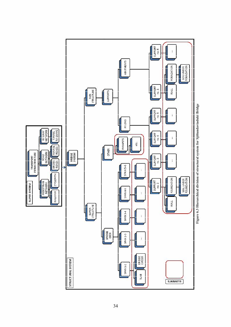
34

Figu

re 6

.3 H

iera

rchi

cal d

ivis

ion

of st

ruct

ural

syst

em fo

r Sj

ölun

davi

aduk

t Bri

dge

35

Other important characteristics of the bridge system are the properties attributed to its constituent elements such as material and geometric features. This includes the concrete quality of various elements, the steel reinforcement, post-tensioning cables, bearing systems etc. However, the characteristics of the external and internal perturbations (i.e. different types of loading and internal flaws) are also significant in that they can directly affect the attributes of the structural elements. By this it is meant that the probability of failure of a structural member is largely dependent on its actual internal circumstance (i.e. is it flawed in some way) as well as the relevant external perturbations to which it is exposed. It is, however, more difficult to graphically interpret these circumstances in a concise manner but one may refer to section 3 for reference.

Figure 6.4 Graphical representation of couplings/interrelations between elements in Sjölundaviadukt Bridge

The intended function of the bridge system in this case is to maintain the flow of traffic which is a direct attribute of the infrastructure network super-system; i.e. road, pedestrian and cycle traffic on the bridge deck itself as well as train and vehicle traffic underneath the bridge. Another inherent function of the bridge system is to provide a safe environment for its users including rail guards to prevent vehicles from leaving the bridge deck in the event of a traffic accident. It will be prescribed that the failure of two or more of the span sections of the bridge deck constitutes a global failure of the structural system; this can be justified for a relatively small multi-span bridge such as the Sjölundaviadukt Bridge. Furthermore, the failure of a span section would also retard traffic both under the bridge as well as over it which is a direct consequence to the surrounding infrastructure elements.

SPAN 4‐5

SUPPORTno. 2

SUPPORTno. 1

SPAN 1‐2 SPAN 2‐3 SPAN 3‐4

SUPPORTno. 3

SPAN 5‐6

SUPPORTno. 4

SOIL SOILSOILSOIL SOIL

SUPPORTno. 5

BACK

FILL

BACK

FILL

SUPPORTno. 6

SOIL

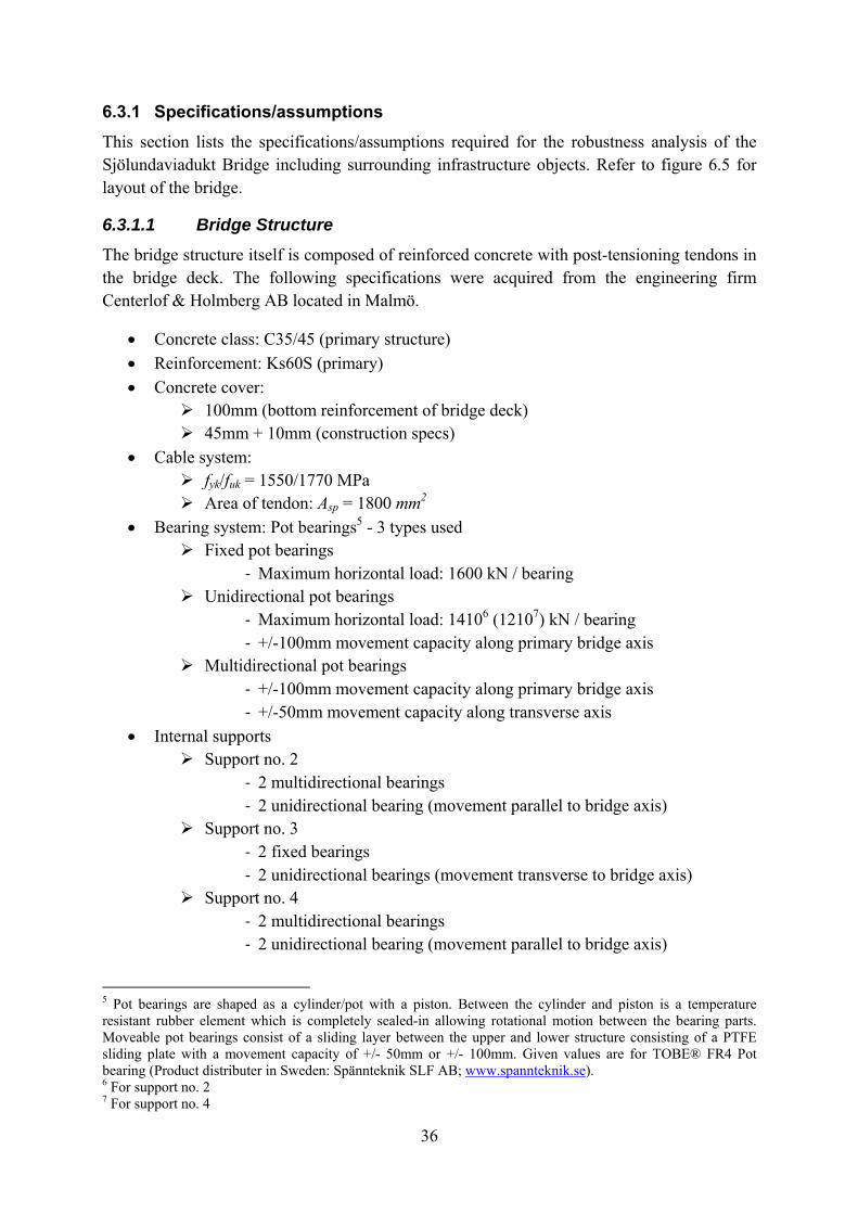
36

6.3.1 Specifications/assumptions This section lists the specifications/assumptions required for the robustness analysis of the Sjölundaviadukt Bridge including surrounding infrastructure objects. Refer to figure 6.5 for layout of the bridge.

6.3.1.1 Bridge Structure The bridge structure itself is composed of reinforced concrete with post-tensioning tendons in the bridge deck. The following specifications were acquired from the engineering firm Centerlof & Holmberg AB located in Malmö.

• Concrete class: C35/45 (primary structure) • Reinforcement: Ks60S (primary) • Concrete cover:

100mm (bottom reinforcement of bridge deck) 45mm + 10mm (construction specs)

• Cable system: fyk/fuk = 1550/1770 MPa Area of tendon: Asp = 1800 mm2

• Bearing system: Pot bearings5 - 3 types used Fixed pot bearings

‐ Maximum horizontal load: 1600 kN / bearing Unidirectional pot bearings

‐ Maximum horizontal load: 14106 (12107) kN / bearing ‐ +/-100mm movement capacity along primary bridge axis

Multidirectional pot bearings ‐ +/-100mm movement capacity along primary bridge axis ‐ +/-50mm movement capacity along transverse axis

• Internal supports Support no. 2

‐ 2 multidirectional bearings ‐ 2 unidirectional bearing (movement parallel to bridge axis)

Support no. 3 ‐ 2 fixed bearings ‐ 2 unidirectional bearings (movement transverse to bridge axis)

Support no. 4 ‐ 2 multidirectional bearings ‐ 2 unidirectional bearing (movement parallel to bridge axis)

5 Pot bearings are shaped as a cylinder/pot with a piston. Between the cylinder and piston is a temperature resistant rubber element which is completely sealed-in allowing rotational motion between the bearing parts. Moveable pot bearings consist of a sliding layer between the upper and lower structure consisting of a PTFE sliding plate with a movement capacity of +/- 50mm or +/- 100mm. Given values are for TOBE® FR4 Pot bearing (Product distributer in Sweden: Spännteknik SLF AB; www.spannteknik.se). 6 For support no. 2 7 For support no. 4

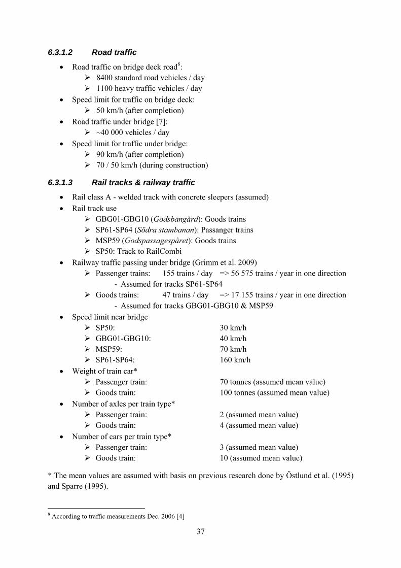
37

6.3.1.2 Road traffic

• Road traffic on bridge deck road8: 8400 standard road vehicles / day 1100 heavy traffic vehicles / day

• Speed limit for traffic on bridge deck: 50 km/h (after completion)

• Road traffic under bridge [7]: ~40 000 vehicles / day

• Speed limit for traffic under bridge: 90 km/h (after completion) 70 / 50 km/h (during construction)

6.3.1.3 Rail tracks & railway traffic

• Rail class A - welded track with concrete sleepers (assumed) • Rail track use

GBG01-GBG10 (Godsbangård): Goods trains SP61-SP64 (Södra stambanan): Passanger trains MSP59 (Godspassagespåret): Goods trains SP50: Track to RailCombi

• Railway traffic passing under bridge (Grimm et al. 2009) Passenger trains: 155 trains / day => 56 575 trains / year in one direction

‐ Assumed for tracks SP61-SP64 Goods trains: 47 trains / day => 17 155 trains / year in one direction

‐ Assumed for tracks GBG01-GBG10 & MSP59 • Speed limit near bridge

SP50: 30 km/h GBG01-GBG10: 40 km/h MSP59: 70 km/h SP61-SP64: 160 km/h

• Weight of train car* Passenger train: 70 tonnes (assumed mean value) Goods train: 100 tonnes (assumed mean value)

• Number of axles per train type* Passenger train: 2 (assumed mean value) Goods train: 4 (assumed mean value)

• Number of cars per train type* Passenger train: 3 (assumed mean value) Goods train: 10 (assumed mean value)

* The mean values are assumed with basis on previous research done by Östlund et al. (1995) and Sparre (1995).

8 According to traffic measurements Dec. 2006 [4]

38

Figu

re 6

.5 G

ener

al la

yout

of

Sjöl

unda

viad

ukt B

ridg

e an

d su

rrou

ndin

g in

fras

truc

ture

(sho

wn

with

per

mis

sion

from

Cen

terl

of &

Hol

dmbe

rg)

39

6.4 Hazard scenarios As with any structural bridge system the relevant hazard scenarios underestimated, overlooked or neglected during the design process must be examined with regard to the structural robustness of the system. Unforeseen hazards are by definition, however, hard to identify and quantify. An attempt may be made following the division given in section 3 in which internal and external perturbations could be considered.

For the sake of simplification it is assumed that the bridge is constructed as designed and that gross internal flaws during design, construction and operation may be neglected. Furthermore it is assumed that no extraordinary exposures occur during the construction of the bridge system. That leaves the external perturbations to be considered for the completed bridge structure. These may be divided as shown in section 3.3:

Overloading ‐ The case of overloading for the Sjölundaviadukt Bridge will be omitted for this

analysis. It seems highly unlikely that at any one time the bridge will contain enough heavy traffic simultaneously to exceed the load carrying capacity of the bridge system.

Accidents ‐ The accidental loading hazard scenario seems more likely in this case in which

traffic collisions to one of the supports from either trains or cars underneath the bridge may cause disproportionate collapse. Traffic on the superstructure (i.e. the road traffic on the bridge itself), however, is much less significant in that the primary structural members for the bridge system are part of the substructure of the bridge according to the hierarchical structural division shown in figure 6.3.

Fatigue/deterioration ‐ It may be assumed that over time the effects of fatigue and deterioration could

significantly alter the robustness of the bridge, however, a thorough and periodic inspection and maintenance of the structure should aid in eliminating any extreme deviations from occurring.

Malevolence (purposeful destruction) ‐ In the case of the Sjölundaviadukt Bridge the primary structural members are

easy to identify. The purposeful destruction of one or more of these members should be taken into consideration. This may be done through analysis of the consequences of removal of one of these members including dynamic effects of explosions, etc, to the system as a whole.

Natural events ‐ This hazard scenario is much harder to identify. Extreme natural events are

very unlikely to occur in the region of the bridge and events such as earthquakes may be neglected altogether. It is also unlikely that flooding would occur although in such a case the surrounding infrastructure networks would be directly affected in any case and the survival of the bridge structure itself becomes second to the safety of its users.

40

In the case of the Sjölundaviadukt the obvious extraordinary exposures include those originating within the super-system; in this case the railway tracks and roads in the surrounding environment. These hazard scenarios are included within the accidental loading set described above. From observation of the layout of the bridge it is determined that the critical elements include the supports for the bridge structure and their failure may lead to indirect consequences for the bridge system as a whole. Thus accidental situations including train or vehicle collisions to one of the bridge supports should be considered. In this paper the former case will be more closely analyzed.

It is important to note that the results obtained from a robustness analysis of a single exposure type do not conclusively determine whether or not the structure is sufficiently robust. It does, however, aid in determining the structural system’s ability to withstand possible failure of one element; i.e. if a critical member (pylon in this case) fails, how will the system react.

In the case of train derailment and subsequent pylon collision an event tree may be formulated based on Baker et al. (2006), refer to figure 6.6. The direct and indirect risks associated with this exposure could be obtained using equations (5.5a) and (5.5b) and an index of robustness evaluated using equation (5.6). The focus of this case study will, however, be on the probabilities associated with the collapse equation given in equation (3.1). The consequences associated with pylon collision as a result of train derailment (i.e. CDir and CInd) will not be quantified.

Figure 6.6 Event tree for train collision with bridge support as a result of derailment

41

6.5 Method of analysis The probability of train derailment, its impact on the bridge supports given collision and the resulting structural consequences to the bridge system as a whole will be examined. A probabilistic method of analysis will be used. The focus of the robustness analysis will be of the probabilities associated with the collapse of the bridge structure.

The event tree shown in figure 6.6 forms the basis for the analysis which will be done. The event exposure being investigated is pylon collision due to derailment of a train towards a supporting member of the bridge deck. This is only one of a variety of exposures which can be accounted for; others may include car/truck collision, explosions, sabotage, etc. The probability associated with the event will be determined and the effect to the support in question analyzed. Finally any indirect effects to the entire structural system can be determined; i.e. will the system fail and to what degree? This does not, however, include any quantification of the consequences to the system, direct or indirect, which would be required in order to calculate an index of robustness according to Baker et al. (2006); see equations (5.5a), (5.5b) and (5.6).

Figure 6. shows a flow chart for the procedure which will be utilized for the robustness analysis of the Sjölundaviadukt Bridge.

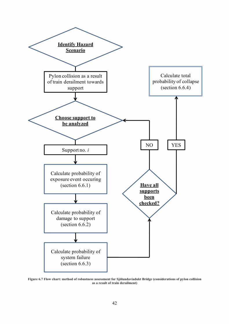
42

Figure 6.7 Flow chart: method of robustness assessment for Sjölundaviadukt Bridge (considerations of pylon collision as a result of train derailment)

Identify Hazard Scenario

Choose support to be analyzed

Calculate probability of exposure event occuring

(section 6.6.1)

Calculate probability of damage to support

(section 6.6.2)

Calculate probability of system failure(section 6.6.3)

Have all supports

been checked?

Pylon collision as a result of train derailment towards

support

Support no. iNO

Calculate total probability of collapse

(section 6.6.4)

YES

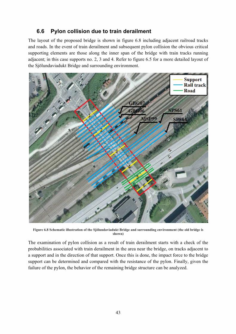
6.6The layand roadsupportiadjacenthe Sjöl

Figure

The exaprobabia supposupport failure o

6 Pylonyout of the ds. In the eving elemen

nt; in this calundaviaduk

e 6.8 Schematic

amination olities associ

ort and in thcan be det

of the pylon

n collisioproposed bvent of train

nts are thosease supportskt Bridge an

c illustration o

of pylon coliated with tre direction ermined an

n, the behav

on due tobridge is shn derailmene along thes no. 2, 3 annd surround

f the Sjölunda

llision as a rain derailmof that supp

nd comparedvior of the re

43

o train deown in figunt and subsee inner spannd 4. Refer tding environ

aviadukt Bridgshown)

result of trment in the port. Once td with the remaining br

erailmenure 6.8 inclequent pylon of the brito figure 6.

nment.

ge and surroun

rain derailmarea near ththis is done,resistance oridge structu

t luding adjac

on collision idge with t5 for a mor

nding environm

ment starts whe bridge, o, the impact

of the pylonure can be a

cent railroathe obvious

train tracks re detailed l

ment (the old b

with a checn tracks adjt force to th

n. Finally, ganalyzed.

ad tracks s critical running

layout of

ridge is

ck of the jacent to

he bridge given the

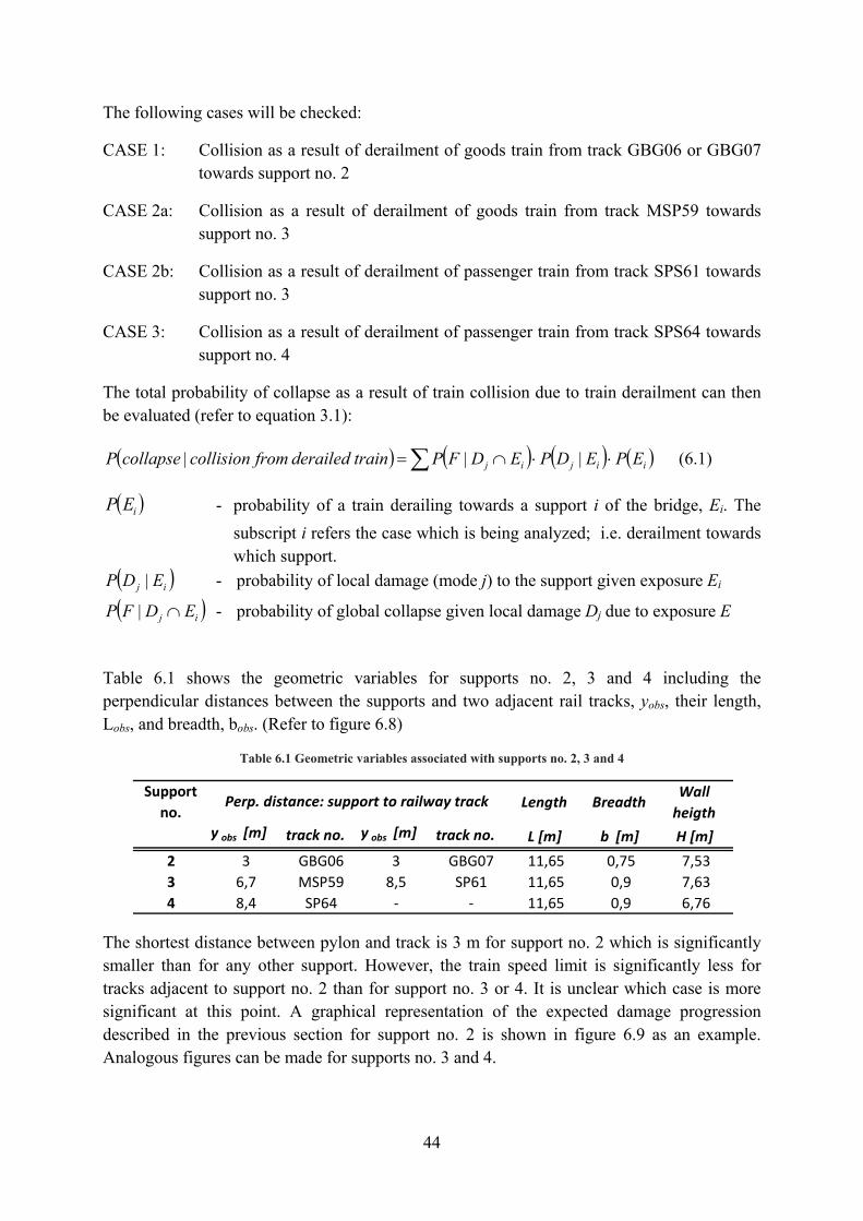
44

The following cases will be checked:

CASE 1: Collision as a result of derailment of goods train from track GBG06 or GBG07 towards support no. 2

CASE 2a: Collision as a result of derailment of goods train from track MSP59 towards support no. 3

CASE 2b: Collision as a result of derailment of passenger train from track SPS61 towards support no. 3

CASE 3: Collision as a result of derailment of passenger train from track SPS64 towards support no. 4

The total probability of collapse as a result of train collision due to train derailment can then be evaluated (refer to equation 3.1):

( ) ( ) ( ) ( )∑ ⋅⋅∩= iijij EPEDPEDFPtrainderailedfromcollisioncollapseP ||| (6.1)

( )iEP - probability of a train derailing towards a support i of the bridge, Ei. The subscript i refers the case which is being analyzed; i.e. derailment towards which support.

( )ij EDP | - probability of local damage (mode j) to the support given exposure Ei

( )ij EDFP ∩| - probability of global collapse given local damage Dj due to exposure E

Table 6.1 shows the geometric variables for supports no. 2, 3 and 4 including the perpendicular distances between the supports and two adjacent rail tracks, yobs, their length, Lobs, and breadth, bobs. (Refer to figure 6.8)

Table 6.1 Geometric variables associated with supports no. 2, 3 and 4

The shortest distance between pylon and track is 3 m for support no. 2 which is significantly smaller than for any other support. However, the train speed limit is significantly less for tracks adjacent to support no. 2 than for support no. 3 or 4. It is unclear which case is more significant at this point. A graphical representation of the expected damage progression described in the previous section for support no. 2 is shown in figure 6.9 as an example. Analogous figures can be made for supports no. 3 and 4.

Support no.

Length BreadthWall heigth

y obs  [m] track no. y obs [m] track no. L [m] b  [m] H [m]2 3 GBG06 3 GBG07 11,65 0,75 7,533 6,7 MSP59 8,5 SP61 11,65 0,9 7,634 8,4 SP64 ‐ ‐ 11,65 0,9 6,76

Perp. distance: support to railway track

45

Figu

re 6

.9 D

amag

e pr

ogre

ssio

n fo

r py

lon

colli

sion

from

trai

n de

railm

ent f

or su

ppor

t no.

2

46

6.6.1 Probability of train derailment in direction towards support The probability of a train leaving the tracks in a direction towards a support of the bridge structure can be determined with the aid of probabilistic derailment models developed by Banverket (Swedish National Railway Authority) (Fredén 2001). The total probability that a train derails towards one of the supporting members of the Sjölundaviadukt Bridge is given by the following equation:

( ) ( ) 3210 PPPPpportsutowardsderailmentPEP ⋅⋅⋅== (6.2)

where:

P0 is the probability of a train derailing in the region near the bridge (arbitrary track length equal to 1 km)

P1 is the probability, given derailment, that a train will derail on tracks adjacent to the support being analyzed

P2 is the probability, given derailment of a train on tracks adjacent to the support being analyzed, that a train will derail in the direction of the support

P3 is the probability, given derailment of a train on tracks adjacent to the support in the direction of the support, that a train will derail within the critical region of collision (see following sections)

Figure 6.10 shows a schematic representation of these probabilities.

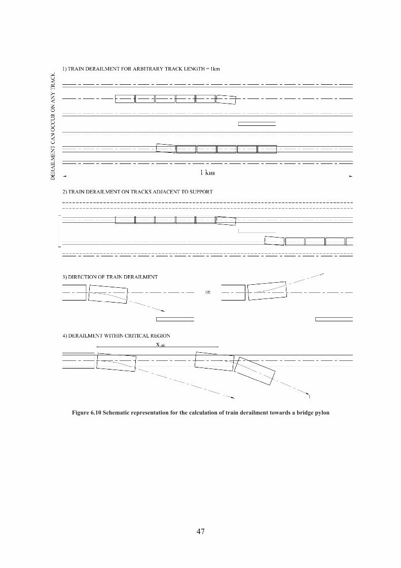
47

Figure 6.10 Schematic representation for the calculation of train derailment towards a bridge pylon

48

The first probability term, P0 and the fourth probability term, P3, must be more closely analyzed. The probability of derailment, P0, can be acquired using calculation models from Banverket (Fredén 2001). The critical region of pylon collision depends on the mechanics of derailment and determines the fourth probability term, P3.

The critical region for pylon collision is defined as the length of track for which, if derailment were to occur, collision is possible. The critical length, xcrit, for an arbitrary derailed train is shown in figure 6.11.

Figure 6.11 Critical region of derailment with regard to train collision with obstruction

It is assumed that a limiting derailment angle exists for which train derailment does not pose a threat for pylon collision. Analogously, a maximum derailment angle is assumed. The minimum derailment angle, θmin, is determined from the maximum stopping distance for a derailed train towards an obstruction alongside the rail tracks while the maximum derailment angle, θmax, is determined for a given speed in which toppling (i.e. rolling over during derailment) of the train is possible. The critical length is then determined from the following formula:

( ) ( )maxmin tantan θθobsobsobs

obscritybyLx −

++= (6.3)

Although complex calculation models may be formulated to examine the mechanism of train derailment (see Brabie 2007) they are quite cumbersome and require a significant amount of input data and complex calculation to apply. Furthermore, many of these models seem rather to focus on methods of preventing derailment rather than on post-derailment behavior and its consequences. Thus a simplified method will be adopted based on Östlund et al (1995). Refer to appendix A for a summary of their findings including calculations of the critical lengths given by equation (6.3).

49

The following formulas were determined for the minimum and maximum derailment angles (see appendix A):

mradCwhere

vC sec.5,3,

0max =≈θ (6.4)

20

1min

2sinv

gyobs ⋅⋅= − ηθ (6.5)

where

C is a constant used to determine the maximum derailment angle, θmax

v0 is the initial velocity of the train as it derails

η is the friction coefficient of the surrounding soil

g is the acceleration due to gravity = 9,8 m/s2

Table 6.2 shows the values for the minimum and maximum derailment angles and critical length of derailment for supports no. 2, 3 and 4. Refer to figure 6.5 and figure 6.8 for a layout of the Sjölundaviadukt Bridge and surrounding railroad tracks.

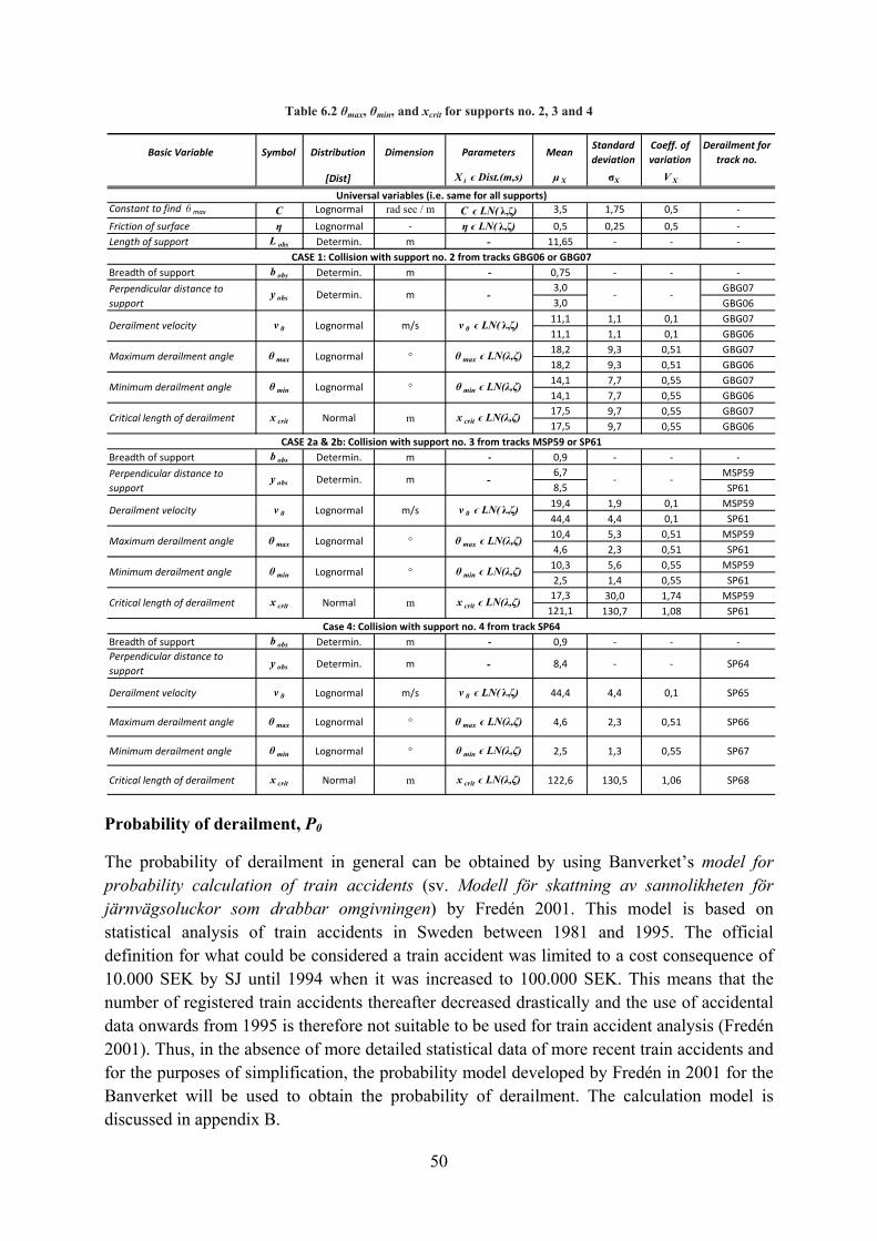
50

Table 6.2 θmax, θmin, and xcrit for supports no. 2, 3 and 4

Probability of derailment, P0

The probability of derailment in general can be obtained by using Banverket’s model for probability calculation of train accidents (sv. Modell för skattning av sannolikheten för järnvägsoluckor som drabbar omgivningen) by Fredén 2001. This model is based on statistical analysis of train accidents in Sweden between 1981 and 1995. The official definition for what could be considered a train accident was limited to a cost consequence of 10.000 SEK by SJ until 1994 when it was increased to 100.000 SEK. This means that the number of registered train accidents thereafter decreased drastically and the use of accidental data onwards from 1995 is therefore not suitable to be used for train accident analysis (Fredén 2001). Thus, in the absence of more detailed statistical data of more recent train accidents and for the purposes of simplification, the probability model developed by Fredén in 2001 for the Banverket will be used to obtain the probability of derailment. The calculation model is discussed in appendix B.

Basic Variable Symbol Distribution Dimension Parameters MeanStandard deviation

Coeff. of variation

Derailment for track no.

[Dist] X i ϵ Dist.(m,s) μ X σX V X

Constant to find  θ max C Lognormal rad sec / m C ϵ LN( λ,ζ) 3,5 1,75 0,5 ‐Friction of surface η Lognormal ‐ η ϵ LN( λ,ζ) 0,5 0,25 0,5 ‐Length of support L obs Determin. m - 11,65 ‐ ‐ ‐

Breadth of support b obs Determin. m ‐ 0,75 ‐ ‐ ‐3,0 GBG073,0 GBG0611,1 1,1 0,1 GBG0711,1 1,1 0,1 GBG0618,2 9,3 0,51 GBG0718,2 9,3 0,51 GBG0614,1 7,7 0,55 GBG0714,1 7,7 0,55 GBG0617,5 9,7 0,55 GBG0717,5 9,7 0,55 GBG06

Breadth of support b obs Determin. m ‐ 0,9 ‐ ‐ ‐6,7 MSP598,5 SP6119,4 1,9 0,1 MSP5944,4 4,4 0,1 SP6110,4 5,3 0,51 MSP594,6 2,3 0,51 SP6110,3 5,6 0,55 MSP592,5 1,4 0,55 SP6117,3 30,0 1,74 MSP59121,1 130,7 1,08 SP61

Breadth of support b obs Determin. m ‐ 0,9 ‐ ‐ ‐Perpendicular distance to support

y obs Determin. m - 8,4 ‐ ‐ SP64

Derailment velocity v 0 Lognormal m/s v 0 ϵ LN( λ,ζ) 44,4 4,4 0,1 SP65

Maximum derailment angle θ max Lognormal ° θ max ϵ LN(λ,ζ) 4,6 2,3 0,51 SP66

Minimum derailment angle θ min Lognormal ° θ min ϵ LN(λ,ζ) 2,5 1,3 0,55 SP67

Critical length of derailment x crit Normal m x crit ϵ LN(λ,ζ) 122,6 130,5 1,06 SP68

Case 4: Collision with support no. 4 from track SP64

Maximum derailment angle θ max Lognormal ° θ max ϵ LN(λ,ζ)

Minimum derailment angle θ min Lognormal ° θ min ϵ LN(λ,ζ)

Critical length of derailment x crit Normal m x crit ϵ LN(λ,ζ)

‐

Derailment velocity v 0 Lognormal m/s v 0 ϵ LN( λ,ζ)

Perpendicular distance to support

y obs Determin. m - ‐

θ max Lognormal ° θ max ϵ LN(λ,ζ)

Critical length of derailment x crit Normal m x crit ϵ LN(λ,ζ)

Minimum derailment angle θ min Lognormal ° θ min ϵ LN(λ,ζ)

CASE 1: Collision with support no. 2 from tracks GBG06 or GBG07

CASE 2a & 2b: Collision with support no. 3 from tracks MSP59 or SP61

Universal variables (i.e. same for all supports)

Perpendicular distance to support

y obs Determin. m - ‐ ‐

Derailment velocity v 0 Lognormal m/s v 0 ϵ LN( λ,ζ)

Maximum derailment angle

51

Probability of derailment on tracks near to support, P1

The probability of derailment on tracks adjacent to a support can easily be determined. It is the ratio of adjacent tracks to the total number of tracks and the same expression can be used for all inner supports, provided that all tracks have the same traffic intensity:

)(..

1 typetraintracksofnototaltracksadjacentofnoP = (6.6)

Probability of derailment in direction of support, P2

The train may derail in two directions off the track and considering that the track is straight in the region being considered:

5,02 =P (6.7)

Probability of derailment within critical region of pylon collision, P3

The probability of derailment within the critical region of pylon collision is determined from the following expression:

kmkmxP critxcrit

113

μ≈= (6.8)

Although the critical region determined from eq. (6.3) is a random variable (refer to table 4.1 and appendix A), the mean value will be used for simplification; i.e. xcrit will be treated as a deterministic variable, for the purposes of determining P3.

Results: Probability of train derailing towards support

Now that all probability terms from equation (6.2) have been determined, the total probability of a train derailing towards supports no. 2, 3 and 4 of the Sjölundaviadukt Bridge can be evaluated. Table 6.3 shows the calculated probabilities associated with each of these supports and the total probability which is calculated using equation (6.2).

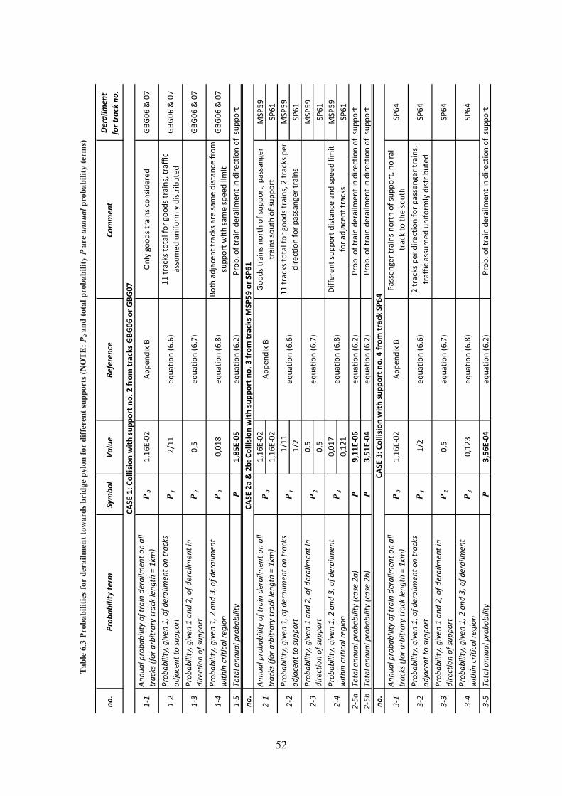
52

T

able

6.3

Pro

babi

litie

s for

der

ailm

ent t

owar

ds b

ridg

e py

lon

for

diff

eren

t sup

port

s (N

OT

E: P

0 and

tota

l pro

babi

lity

P ar

e an

nual

pro

babi

lity

term

s)

no.

Prob

ability te

rmSymbo

lVa

lue

Reference

Commen

tDerailm

ent 

for track no.

1‐5

Total ann

ual proba

bility

P1,85

E‐05

equatio

n (6.2)

no.

1,16

E‐02

MSP59

1,16

E‐02

SP61

1/11

MSP59

1/2

SP61

0,5

MSP59

0,5

SP61

0,01

7MSP59

0,12

1SP61

2‐5a

Total ann

ual proba

bility (case 2a

)P

9,11

E‐06

equatio

n (6.2)

2‐5b

Total ann

ual proba

bility (case 2b

)P

3,51

E‐04

equatio

n (6.2)

no.

3‐5

Total ann

ual proba

bility

P3,56

E‐04

equatio

n (6.2)

CASE 1: C

ollision  with

 sup

port no. 2 from

 tracks GBG

06 or G

BG07

1‐1

1‐2

1‐3

1‐4

Annu

al proba

bility of train derailm

ent o

n all 

tracks (for arbitrary track leng

th = 1km

)P

0Ap

pend

ix B

Goo

ds trains north of sup

port, passanger 

trains so

uth of su

pport

2‐1

Prob

ability, given

 1 and

 2, of d

erailm

ent in 

direction of su

pport

P2

Prob

ability, given

 1, 2

 and

 3, of d

erailm

ent 

with

in critical re

gion

P3

CASE 2a & 2b: Collision with

 sup

port no. 3 from

 tracks M

SP59

 or S

P61

1,16

E‐02

  2/11

GBG

06 & 07

Annu

al proba

bility of train derailm

ent o

n all 

tracks (for arbitrary track leng

th = 1km

)P

0Ap

pend

ix B

Prob

ability, given

 1, of d

erailm

ent o

n tracks 

adjacent to

 supp

ort

P1

GBG

06 & 07

GBG

06 & 07

Both adjacen

t tracks a

re sam

e distance from

 supp

ort w

ith sa

me speed lim

it

Only good

s trains c

onsid

ered

equatio

n (6.6)

11 tracks to

tal for goo

ds trains, traffic 

assumed

 uniform

ly distrib

uted

GBG

06 & 07

0,5

equatio

n (6.7)

equatio

n (6.8)

0,01

8

2‐4

equatio

n (6.8)

Diffe

rent su

pport d

istance and

 speed lim

it for a

djacen

t tracks

2‐2

equatio

n  (6.6)

11 tracks to

tal for goo

ds trains, 2

 tracks per 

direction for p

assanger trains

Prob

ability, given

 1, of d

erailm

ent o

n tracks 

adjacent to

 supp

ort

P1

Prob

ability, given

 1 and

 2, of d

erailm

ent in 

direction of su

pport

P2

Prob

ability, given

 1, 2

 and

 3, of d

erailm

ent 

with

in critical re

gion

P3

3‐3

Prob

ability, given

 1 and

 2, of d

erailm

ent in 

direction of su

pport

P2

equatio

n (6.7)

Prob

. of train derailm

ent in direction of  sup

port

Prob

. of train derailm

ent in direction of  sup

port

3‐2

Prob

ability, given

 1, of d

erailm

ent o

n tracks 

adjacent to

 supp

ort

P1

equatio

n (6.6)

2 tracks per dire

ction for p

assenger trains, 

traffic assum

ed uniform

ly distrib

uted

CASE 3: C

ollision with

 sup

port no. 4 from

 track SP64

3‐1

Annu

al proba

bility of train derailm

ent o

n all 

tracks (for arbitrary track leng

th = 1km

)P

0Ap

pend

ix B

Passen

ger trains n

orth of sup

port, no rail 

track to th

e south

2‐3

equatio

n (6.7)

Prob

. of train derailm

ent in direction of  sup

port

3‐4

Prob

ability, given

 1, 2

 and

 3, of d

erailm

ent 

with

in critical re

gion

P3

equatio

n (6.8)

0,12

3SP64

Prob

. of train derailm

ent in direction of  sup

port

1,16

E‐02

1/2

0,5

SP64

SP64

SP64

53

6.6.2 Direct consequences of pylon collision The behavior of a derailed train has been discussed as well as the probability of such an event occurring. The next step is then to analyze the direct structural consequences of a train colliding with a bridge support; i.e. how will the pylon be directly affected. This entails determining a collision force to the pylon (refer to appendix A) as well as checking the resistance of the support for different failure modes.

6.6.2.1 Action effect – force from collision The calculation of the force at impact for a derailed train may be obtained using complex crash mechanics. However, these calculations are quite complex and will not be used for the purposes of this paper*. Instead a simplified model based on traditional physical relations will be adopted. Refer to appendix A for calculations relevant to the derailment model which is to be used.

* The focus of this paper is on creating a framework for the assessment of robustness of bridges rather than on the specific methods of analysis. It must be noted, however, that in the case of a more thorough structural robustness case study, more complex analytical procedures may be required.

Force at impact, Fimp The force at impact, Fimp, for a derailed train when it collides with a bridge pylon is dependent on the train’s velocity at impact (refer to appendix A). Two simplified methods for determining this force will be considered based on (1) impulse momentum equilibrium (equation (6.9a)) and (2) energy equilibrium (equation (6.9b)).

tvm

F impimp Δ

⋅= (6.9a)

Δt – impulse time during collision.

svm

F impimp Δ⋅

⋅=

2

2

(6.9b)

Δs – the distance in which the center of gravity of the body travels during collision; i.e. the “shortening” distance of the train in this case.

Since neither Δt nor Δs can be explicitly determined, suitable estimations must be made. Both variables will be assumed lognormally distributed with the following means and coefficients of variation:

1,05,1 == ΔΔ ss Vmμ

(6.10a)

1,05,0 == ΔΔ tt Vsμ (6.10b)

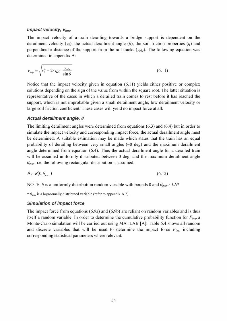
54

Impact velocity, vimp The impact velocity of a train derailing towards a bridge support is dependent on the derailment velocity (v0), the actual derailment angle (θ), the soil friction properties (η) and perpendicular distance of the support from the rail tracks (yobs). The following equation was determined in appendix A:

θη

sin22

0obs

impygvv ⋅⋅−= (6.11)

Notice that the impact velocity given in equation (6.11) yields either positive or complex solutions depending on the sign of the value from within the square root. The latter situation is representative of the cases in which a derailed train comes to rest before it has reached the support, which is not improbable given a small derailment angle, low derailment velocity or large soil friction coefficient. These cases will yield no impact force at all.

Actual derailment angle, θ

The limiting derailment angles were determined from equations (6.3) and (6.4) but in order to simulate the impact velocity and corresponding impact force, the actual derailment angle must be determined. A suitable estimation may be made which states that the train has an equal probability of derailing between very small angles (~0 deg) and the maximum derailment angle determined from equation (6.4). Thus the actual derailment angle for a derailed train will be assumed uniformly distributed between 0 deg. and the maximum derailment angle θmax; i.e. the following rectangular distribution is assumed:

( )max,0 θθ R∈ (6.12)

NOTE: θ is a uniformly distribution random variable with bounds 0 and θmax ϵ LN*

* θmax is a lognormally distributed variable (refer to appendix A.2).

Simulation of impact force

The impact force from equations (6.9a) and (6.9b) are reliant on random variables and is thus itself a random variable. In order to determine the cumulative probability function for Fimp a Monte-Carlo simulation will be carried out using MATLAB [A]. Table 6.4 shows all random and discrete variables that will be used to determine the impact force Fimp including corresponding statistical parameters where relevant.

55

Table 6.4 Basic variables used for calculation of impact force

Now that all parameters required to calculate the impact force have been determined, along with their corresponding statistical attributes, the Monte Carlo simulation may be used to determine the distribution of Fimp. Figure 6.12 shows the results for 1 000 000 simulations for equations (6.9a) and (6.9b) for support no. 2.

Basic Variable Symbol Distribution Dimension Parameters meanCoeff. of variation

[Dist] X i ϵ Dist.(m,s) μ X V X

Mass of train m Normal tonnes m ϵ N(μ,σ) sec. 6.3.1.1 0,1Derailment velocity v 0 Lognormal m/s v 0 ϵ LN( λ,ζ) sec. 6.3.1.1 0,1Actual derailment angle θ Uniform ° θ ϵ R(0,θ max ) varies variesMaximum derailment angle θ max eq. (6.3) ° θ max = C/v 0 ‐ ‐Constant to find  θ max C Lognormal rad sec / m C ϵ LN( λ,ζ) 3,5 0,5Perpendicular distance to support

y obs Determin. m - table 6.1‐

Shortening  Δs Lognormal m Δs ϵ LN( λ,ζ) 1,5 0,1Impulse time Δt Lognormal s Δt ϵ LN( λ,ζ) 0,5 0,1Friction of surface η Lognormal ‐ η ϵ LN( λ,ζ) 0,5 0,5

56

Figure 6.12 Impact force for support no. 2 (case 1)

Notice that there exists a probability of about 53% that for derailment of a train in the direction towards support no. 2 the train it will stop before it can cause a collision. It is therefore not so simple to attain a valid statistical distribution for the empirical distribution shown in figure 6.12 without transforming the empirical distribution.

Although both curves from figure 6.12 yield similar distributions the curve created using equation (6.9b) will be utilized for use in further analysis; i.e. based on “shortening” of train during impact (Δs). Figure 6.13 and figure 6.14 show the empirical distribution for the perpendicular impact force component (i.e. orthogonal to support wall) for derailed trains toward supports no. 3 and 4 using equation (6.9b).

The next step is to determine the resistance of the support against collision.

57

Figure 6.13 Perpendicular impact force component for collision with support no. 3 from goods trains (case 2a) and commuter trains (case 2b)

Figure 6.14 Perpendicular impact force component for collision with support no. 4 from commuter trains (case 3)

58

6.6.2.2 Resistance of support In order to extract the probability of failure for the support in the event of a train collision, the corresponding resistance to the impact forces found in section 6.6.2.1 must be determined for cases 1, 2a, 2b and 3 (refer to section 6.6). Thus the parameters pertaining to the strength, material, geometric, etc. properties of the supporting members must be determined along with their statistical attributes. However, first the various failure modes pertaining to a collision with a pylon of the Sjölundaviadukt Bridge must be identified.

The failure modes for a bridge support in the event of collision from a derailed train are given in the following list (refer to figure 6.15):

1. Shear failure at joint between support wall and foundation footing given rotation about bearing connections between bridge and support.

o Mechanism: Friction capacity at section between wall and foundation (including contribution of reinforcement) overcome. It is assumed that the pot bearings do not fail; i.e. support wall does not slide from under bridge during impact.

2. Failure of support wall due to combined moment and axial action given that the bearing connections between bridge and support do not fail.

o Mechanism: Combined axial force from bridge deck and moment due to impact causes failure of wall (i.e. MN graph).

3. Failure of support wall with 2 plastic hinges given that the bearing connections between bridge and support do not fail.

o Mechanism: As for 2 but yield moment capacity at connection between wall and foundation overcome.

4. Failure of support wall due to combined moment and axial action given failure of bearing connection between support and bridge deck.

o Mechanism: Failure of bridge bearings and subsequent combined moment and axial action at the bottom of the wall.

5. Sliding of support foundation and rotation about bearing connection between support and bridge.

o Mechanism: Impact force causes foundation to slide; i.e. shear resistance between foundation and soil overcome while the bearing connection between bridge and support does not fail.

6. Sliding of support foundation and failure of bearing connection between support and bridge deck.

o Mechanism: Impact force cause foundation to slide and bearing connection between bridge and support to fail almost simultaneously.

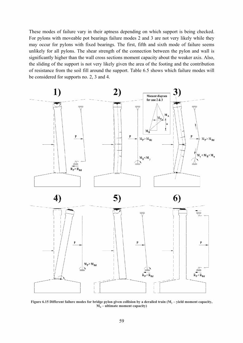
59

These modes of failure vary in their aptness depending on which support is being checked. For pylons with moveable pot bearings failure modes 2 and 3 are not very likely while they may occur for pylons with fixed bearings. The first, fifth and sixth mode of failure seems unlikely for all pylons. The shear strength of the connection between the pylon and wall is significantly higher than the wall cross sections moment capacity about the weaker axis. Also, the sliding of the support is not very likely given the area of the footing and the contribution of resistance from the soil fill around the support. Table 6.5 shows which failure modes will be considered for supports no. 2, 3 and 4.

Figure 6.15 Different failure modes for bridge pylon given collision by a derailed train (My – yield moment capacity, Mu – ultimate moment capacity)

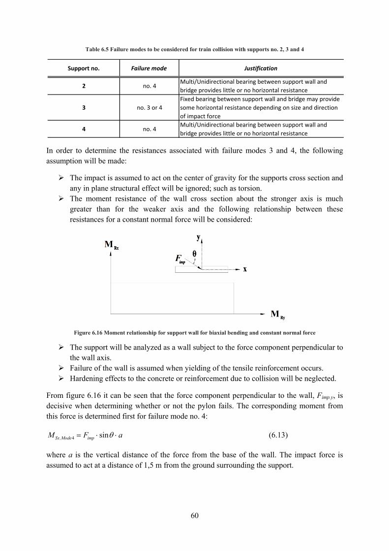
60

Table 6.5 Failure modes to be considered for train collision with supports no. 2, 3 and 4

In order to determine the resistances associated with failure modes 3 and 4, the following assumption will be made:

The impact is assumed to act on the center of gravity for the supports cross section and any in plane structural effect will be ignored; such as torsion.

The moment resistance of the wall cross section about the stronger axis is much greater than for the weaker axis and the following relationship between these resistances for a constant normal force will be considered:

Figure 6.16 Moment relationship for support wall for biaxial bending and constant normal force

The support will be analyzed as a wall subject to the force component perpendicular to the wall axis.

Failure of the wall is assumed when yielding of the tensile reinforcement occurs. Hardening effects to the concrete or reinforcement due to collision will be neglected.

From figure 6.16 it can be seen that the force component perpendicular to the wall, Fimp.y, is decisive when determining whether or not the pylon fails. The corresponding moment from this force is determined first for failure mode no. 4:

aFM impModeSx ⋅⋅= θsin4. (6.13)

where a is the vertical distance of the force from the base of the wall. The impact force is assumed to act at a distance of 1,5 m from the ground surrounding the support.

Support no. Failure mode Justification

2 no. 4Multi/Unidirectional bearing between support wall and bridge provides little or no horizontal resistance

3 no. 3 or 4Fixed bearing between support wall and bridge may provide some horizontal resistance depending on size and direction of impact force

4 no. 4Multi/Unidirectional bearing between support wall and bridge provides little or no horizontal resistance

61

The moment diagram for failure mode no. 3 is shown in figure 6.17. There are two moments which must be considered: MA – moment at location of impact force and MB – moment at connection between the support wall and foundation footing. The superposition method used to determine internal forces and deformations of statically indeterminate linear elastic structures determines the following (refer to figure 6.17):

HaHaFM impP

−⋅⋅⋅= θsin (6.14a)

where H is the height of the wall.

Figure 6.17 Method of superposition to determine the moment distribution for failure mode no. 2

The corresponding resistances to moments MA and MB must be considered for failure mode no. 3: MRAx and MRBx. The following condition is obtained:

PRBxRAx MHaMM ≤⋅+ / (6.14b)

Refer to section 6.6.2.3.

62

Figure 6.18 shows the layout of support no. 2 with regard to pylon collision from a derailed train.

Figure 6.18 Layout for collision with support no. 2 due to train derailment

63

The moment resistance of the support walls for combined uniaxial bending and normal force was determined in appendix C. The following formula was determined:

⎟⎠⎞

⎜⎝⎛ ⋅−⋅⋅⋅⋅⋅+⎟

⎠⎞

⎜⎝⎛ −⋅⋅= xbxLfbdAfM csyRx 4,0

28,0

2α (6.15)

where the depth of the neutral axis (i.e. where strain is zero) is determined:

LfAfN

xc

sy

⋅⋅⋅⋅+

=8,0α

(6.16)

N Normal force on wall from self weight loading only, see table 6.6

fy Yield strength of reinforcing steel, see table 6.7

fc Compressive strength of concrete, see table 6.7

α In-situ parameter for compressive strength of concrete, table 6.7

As Area of tensile reinforcement, see table 6.6

b Height of cross section (wall thickness), see table 6.1

d Depth of tensile reinforcement, see table 6.6

L Breadth of cross section (wall length), see table 6.1

Table 6.6 values for axial and impact loading of supports no. 2, 3 and 4 including reinforcement in walls

In the case of support no. 3, which has fixed bearings between the support wall and bridge, equation (6.13) is permitted only if the reaction due to the impact force does not exceed the combined horizontal force resistances of the fixed pot bearings; i.e. if ∑≤ bearingRbearingimp HR ..

then equation (6.13) applies, otherwise, equation (6.14a) and (6.14b) should be used. The characteristic horizontal force resistances for the pot bearings are given in section 6.3.1.1. The total reaction force at the bearings is given by equation (6.17) (Teknisk Ståbi 2004); refer to figure 6.17.

⎥⎦⎤

⎢⎣⎡ −+⎟

⎠⎞

⎜⎝⎛=

HaH

HaFR impbearingimp 2

21 2

. (6.17)

Support no.

Normal force

Impact Force

Height of impact force

Depth of reinf.

N [MN] F imp  [MN] a [mm] no. x  Ø A s [mm 2 ] d [mm]

2 29,2 fig. 20 2,88 58 Ø25 56 941 7053 27,2 fig. 21 3,05 118* Ø16 47 451 8554 16,3 fig. 22 2,5 118 Ø16 47 451 855

* 234 @ connection between wall & foundations, 118 elsewhere

Tensile reinf.

64

6.6.2.3 Probability of pylon failure given train derailment towards support The resulting impact force from a derailed train has been determined as well as two corresponding failure modes that should be considered. The resistances of the pylons attributed to these failure modes have also been determined. The next step is then to determine the probability of pylon failure given train derailment in the direction of one of the inner bridge support; i.e. case 1 to 3 from section 6.6.

The two failure modes which will be analyzed are due to concrete failure in combined bending and axial action. The difference between the two is in the mechanism of failure; refer to figure 6.15. A limit state equation can be written which prescribes the conditions of failure of these two modes (no. 3 and 4):

SxRx MMSRZ −=−= (6.18a)

or alternatively

θsin. ⋅−=−= impRyyimpRy FFFFZ (6.18b)

where

( )

⎪⎪⎩

⎪⎪⎨

⎧−⋅⋅

=4

3

4

3

Modea

M

ModeaHa

HM

FxR

xR

Ry (6.19)

The moment resistance for mode no. 4 is directly determined from equation (6.15) while the resistance for failure mode no. 3 is determined from expression (6.14b):

)15.6(/

4

3

equationMHaMMM

xR

RBxRAxxR

=

⋅+= (6.20)

The moment terms MRAx and MRBx are determined from equation (6.15); refer to figure 6.17.

The probability of failure of the pylon is determined:

( ) ( ) ( )00| . ≤−=≤= yimpRy FFPZPpylontowardstrainofderailmentfailurepylonP (6.21)

In order to determine the above probability, the statistical parameters of all stochastic input variables must be included. Furthermore, the JCSS Probabilistic Model Code (2001) includes uncertainty parameters for the load effects and resistances to account for model uncertainties; denoted by θE and θR respectively.

65

The limit equation (6.18b) can then be rewritten in the following form:

( ) [ ]θθθθθ sin4

3

4

3

. ⋅⋅−

⎪⎪⎭

⎪⎪⎬

⎫

⎪⎪⎩

⎪⎪⎨

⎧−⋅⋅

⋅=⋅−⋅= impExR

xR

RyimpERyR FModefor

aM

ModeforaHa

HM

FFZ (6.22)

Inputting all basic variables, the full form is obtained for mode 4 (using equations 6.9b, 6.11 & 6.15):

( )⎥⎦⎤

⎢⎣⎡ ⋅⋅⋅−⋅⋅

Δ⋅⋅−

⋅⎥⎦

⎤⎢⎣

⎡⎟⎠⎞

⎜⎝⎛ ⋅−⋅⋅⋅⋅⋅+⎟

⎠⎞

⎜⎝⎛ −⋅⋅⋅=

obsE

csyR

ygvs

ma

xhxbfhdAfZ

ηθθ

αθ

2sin2

14,02

8,02

20

(6.23a)

and mode 3:

[ ] ( )

( )⎥⎦⎤

⎢⎣⎡ ⋅⋅⋅−⋅⋅

Δ⋅⋅−

−⋅⋅⋅+⋅=

obsE

RBxRAxR

ygvs

maHa

HHaMMZ

ηθθ

θ

2sin2

/

20

(6.23b)

A Monte-Carlo simulation can then be done to determine the overall probability of failure. The basic variables that will be used for the probabilistic assessment of pylon failure given train collision are shown in table 6.7. The mean values and coefficients of variation for the basic variables pertaining to the resistance of the wall (see eq. 6.15) in table 6.7 were determined from Carlsson (2002) or assumed based on discussions with Professor Thelandersson and Dr. Carlsson.

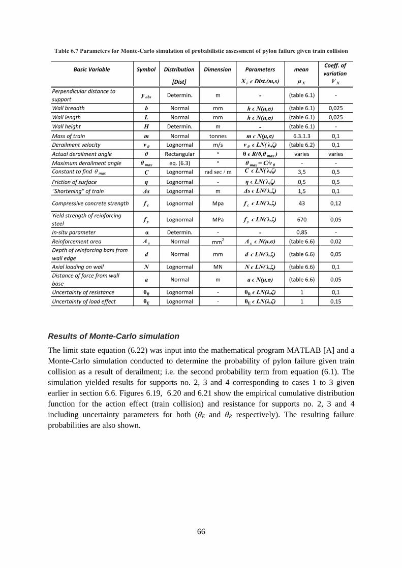
66

Table 6.7 Parameters for Monte-Carlo simulation of probabilistic assessment of pylon failure given train collision

Results of Monte-Carlo simulation The limit state equation (6.22) was input into the mathematical program MATLAB [A] and a Monte-Carlo simulation conducted to determine the probability of pylon failure given train collision as a result of derailment; i.e. the second probability term from equation (6.1). The simulation yielded results for supports no. 2, 3 and 4 corresponding to cases 1 to 3 given earlier in section 6.6. Figures 6.19, 6.20 and 6.21 show the empirical cumulative distribution function for the action effect (train collision) and resistance for supports no. 2, 3 and 4 including uncertainty parameters for both (θE and θR respectively). The resulting failure probabilities are also shown.

Basic Variable Symbol Distribution Dimension Parameters meanCoeff. of variation

[Dist] X i ϵ Dist.(m,s) μ X V X

Perpendicular distance to support

y obs Determin. m - (table 6.1) ‐

Wall breadth b Normal mm h ϵ N(μ,σ) (table 6.1) 0,025Wall length L Normal mm h ϵ N(μ,σ) (table 6.1) 0,025Wall height H Determin. m - (table 6.1) ‐

Mass of train m Normal tonnes m ϵ N(μ,σ) 6.3.1.3 0,1Derailment velocity v 0 Lognormal m/s v 0 ϵ LN( λ,ζ) (table 6.2) 0,1Actual derailment angle θ Rectangular ° θ ϵ R(0,θ max ) varies variesMaximum derailment angle θ max eq. (6.3) ° θ max = C/v 0 ‐ ‐Constant to find  θ max C Lognormal rad sec / m C ϵ LN( λ,ζ) 3,5 0,5

Friction of surface η Lognormal ‐ η ϵ LN( λ,ζ) 0,5 0,5"Shortening" of train Δs Lognormal m Δs ϵ LN( λ,ζ) 1,5 0,1

Compressive concrete strength f c Lognormal Mpa f c ϵ LN( λ,ζ) 43 0,12

Yield strength of reinforcing steel

f y Lognormal MPa f y ϵ LN( λ,ζ) 670 0,05

In‐situ parameter α Determin. ‐ - 0,85 ‐Reinforcement area A s Normal mm2 A s ϵ N(μ,σ) (table 6.6) 0,02Depth of reinforcing bars from wall edge

d Normal mm d ϵ LN( λ,ζ) (table 6.6) 0,05

Axial loading on wall N Lognormal MN N ϵ LN( λ,ζ) (table 6.6) 0,1Distance of force from wall base

a Normal m a ϵ N(μ,σ) (table 6.6) 0,05

Uncertainty of resistance θR Lognormal ‐ θR ϵ LN(λ,ζ) 1 0,1Uncertainty of load effect θE Lognormal ‐ θE ϵ LN(λ,ζ) 1 0,15

67

Figure 6.19 Empirical CDFs for the action effect (train collision) versus resistance for support no. 2

Figure 6.20 Empirical CDFs for the action effect (goods/commuter train collision) versus resistance for support no. 3

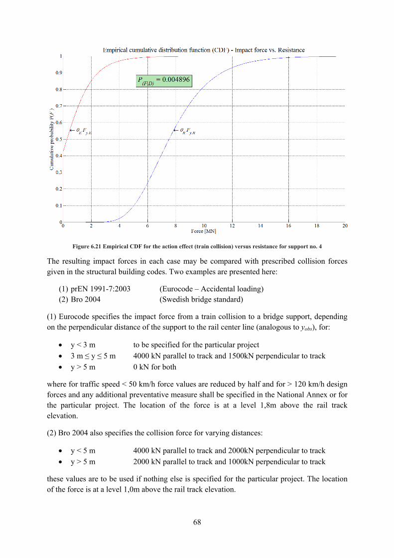
68

Figure 6.21 Empirical CDF for the action effect (train collision) versus resistance for support no. 4

The resulting impact forces in each case may be compared with prescribed collision forces given in the structural building codes. Two examples are presented here:

(1) prEN 1991-7:2003 (Eurocode – Accidental loading) (2) Bro 2004 (Swedish bridge standard)

(1) Eurocode specifies the impact force from a train collision to a bridge support, depending on the perpendicular distance of the support to the rail center line (analogous to yobs), for:

• y < 3 m to be specified for the particular project • 3 m ≤ y ≤ 5 m 4000 kN parallel to track and 1500kN perpendicular to track • y > 5 m 0 kN for both

where for traffic speed < 50 km/h force values are reduced by half and for > 120 km/h design forces and any additional preventative measure shall be specified in the National Annex or for the particular project. The location of the force is at a level 1,8m above the rail track elevation.

(2) Bro 2004 also specifies the collision force for varying distances:

• y < 5 m 4000 kN parallel to track and 2000kN perpendicular to track • y > 5 m 2000 kN parallel to track and 1000kN perpendicular to track

these values are to be used if nothing else is specified for the particular project. The location of the force is at a level 1,0m above the rail track elevation.

69

The recommended values from structural codes may be compared with the 95th and 98th percentile values (for the perpendicular force component) found from the analysis, refer to figures 6.19, 6.20 and 6.21:

(The speed limits and rail distances for these supports are shown in table 6.2.)

SUPPORT 2

• Analysis 95th ~1,1 MN 98th ~1,5 MN • ENV 1991-1-7 750 kN • Bro 2004 2000 kN

SUPPORT 3

• Analysis* 95th ~1,3/3,1 MN 98th ~2,1/3,9 MN • ENV 1991-1-7 0 kN** / specific analysis required (speed > 120 km/h) • Bro 2004 1000 kN for both

* values given for goods/commuter train collision ** since distance between track and rail is greater than 5 m SUPPORT 4

• Analysis 95th ~3,2 MN 98th ~3,9 MN • ENV 1991-1-7 specific analysis required (speed > 120 km/h) • Bro 2004 1000 kN

In all cases the prescribed force in both structural codes is less than what was calculated with the Monte Carlo simulation. Thus in the case of the Sjölundaviadukt Bridge (and based on the results from the mechanical train collision model used in this paper) the inclusion of train impact loading from structural codes in the design procedure does not exclude it as a pertinent hazard scenario to be considered for a robustness analysis. However, it is difficult to arrive at any legitimate conclusion without further investigation. Furthermore, the validity of the mechanical crash model developed in this paper cannot be substantially verified without more complex and thorough analyses.

70

6.6.3 Indirect consequences of pylon collision The previous sections have examined the direct effects of pylon collision as a result of train derailment; i.e. the effects to the support itself. The probability of pylon failure was determined for supports no. 2, 3 and 4. Given that one of these supports fail, the so-called indirect consequences to the bridge system can be analyzed. This involves a check of the residual capacity of the impaired structure. Intuitively it may be observed that the design of the post-tensioned concrete deck for a fully functioning bridge will be decisively inadequate given removal of one of its inner supports. A deterministic analysis will thus be done initially to check the degree of lessened structural integrity given pylon removal. Since the system is no longer static, the dynamic effects of sudden pylon removed must be considered. In absence of any dynamic studies, self-weight will be increased by 50% to account for these effects9; i.e. a dynamic amplification factor of 1.5 will be adopted.

The various failure modes for the bridge deck given pylon removal will be considered. In the event of support removal, the span between the remaining adjacent supports increases resulting in moment redistribution. The first mode of failure for an impaired bridge structure is the failure of the bridge deck in bending. A plastic analysis may be conducted to check the moment capacity of the bridge span given failure of one of its supporting elements. The second failure mode is a continuation of the first. In the event that the bridge deck yields catenary action may aid in retaining some residual load carrying capacity such that the bridge deck does not fail completely. However, the first mode of failure will only be checked in this section of the report.

The behavior of the Sjölundaviadukt Bridge given failure of one of its supports will be examined. The resistance of the bridge deck will be determined given pylon removal for permanent loading only; i.e. self-weight. Table 6.8 shows the effective characteristic distributed line loading of the bridge deck for each span from self weight loading.

Table 6.8 Distributed linear loading of bridge deck for all spans from self-weight (without dynamic factor)

9 According to Schubert et. al 2007, an additional 50% of the normal force that acted on the removed support could be considered. An approximation will be assumed that loading due to dynamic effects will be 50% of the self weight loading of the bridge deck instead.

Span LengthDeck effective 

breadthLoading on bridge*

L [m] b [m] q [kN/m]

1‐2 35,925 13,1 ~5502‐3 50,000 13,1 ~5503‐4 36,000 13,1 ~5504‐5 28,475 13,2 ~4505‐6 22,000 13,2 ~450

* Self weight loading only (characteristic)

71

The moment distribution for a fully functioning bridge may be compared with an impaired bridge structure in which one of the inner supports is removed; i.e. supports no. 2, 3 or 4. Figure 6.23 shows the influence diagram for the moment distribution in the bridge deck for a uniformly distributed load according to table 6.8. The influence lines for an unimpaired and impaired structure (i.e. given pylon removal) are shown. Figure 6.22 shows a typical cross section for the Sjölundaviadukt Bridge.

Figure 6.22 Cross section of the bridge deck for Sjölundaviadukt Bridge.

72

-500

-400

-300

-200

-1000

100

200

300

400

020

4060

8010

012

014

016

0

Moment [MNm]

Loc

atio

n al

ong

brid

ge [m

]

Sjöl

unda

viad

ukt:

Mom

ent d

iagr

am fo

r py

lon

rem

oval

Uni

mpa

ired

stru

ctur

eR

emov

e Su

ppor

t no.

2R

emov

e Su

ppor

t no.

3R

emov

e Su

ppor

t no.

4

q=55

0kN

/mq=

450k

N/m

Figu

re 6

.23

Mom

ent d

iagr

am fo

r Sj

ölun

davi

aduk

t for

func

tioni

ng st

ruct

ure

vs. r

emov

al o

f sup

port

s no.

2, 3

and

4 (d

ynam

ic e

ffec

t of p

ylon

rem

oval

neg

lect

ed)

73

A plastic analysis will be carried out to determine the residual capacity of the bridge deck given removal of supports no. 2, 3 or 4 for loading given in table 6.8. This involves checking the residual moment capacities of the bridge deck for an impaired bridge structure. Two cases are considered:

(1) Removal of the first inner supports nearest to bridge abutments (i.e. support no. 2) (2) Removal of other inner supports (i.e. supports no. 3 and 4)

Figure 6.24 shows the resultant moment distribution for distributed loading q given removal of support no. 2 (case (1)) and 3 (case (2)).

Figure 6.24 Moment distribution along bridge deck for removal of (a) support no. 2 and (b) support no. 3 (dynamic factor not included)

The following condition must then be fulfilled (dynamic factor for load included):

Case (1) 8

5,12

2sup.

.LqM

M RspanR

⋅≤+ (6.23a)

Case (2) 8

5,12

2.sup..sup.

.LqMM

M BRARspanR

⋅≤

++ (6.23b)

a)

b)

74

where the moment resistance of the bridge deck at any given cross section is determined from the ultimate tensile capacity of the post-tensioning cables (refer to appendix D):

spcablesukcablesR AnfdM ⋅⋅⋅⋅= 9.0 (6.24)

Equation (6.24) can then be used with equations (6.23a) or (6.23b) for removal of supports no. 2, 3 or 4 to determine whether or not the residual load carrying capacity of the bridge is exceeded. The cross sectional data, including the number and position of the tendons, for various sections along the Sjölundaviadukt Bridge span is shown in table 6.9.

Table 6.9 Data for cables at various locations along span of Sjölundaviadukt Bridge

Results for residual load carrying capacity of bridge given pylon removal The following results were obtained for the residual load carrying capacity of the bridge deck for removal of supports no. 2, 3 and 4 using equations (6.23a) and (6.23b).

Removal of support no. 2 Effective span length: L = ~86 m

Loading from self weight: q = 550 kN/m

Control: equation (6.23a)

MNmLqMM R

spanR 7638

865505,18

5,12

22313.sup.

31.. ≈⋅

=⋅

≤+ −− (6.25)

Location along bridge

No. of cables

Cable group height

Deck height (at center line)

Description

m ea mm mm

+ 0,000 46 500/911 1400 Support no. 1+ 13,472 46 137 1400 3/8‐span 1‐2+ 35,925 58 ~2200 2400 Support no. 2+ 42,963 76 ~900 ~1500 Mid‐span 1‐3+ 60,925 88 137 1400 Mid‐span 2‐3+ 78,925 70 ~770 ~1500 Mid‐span 2‐4+ 85,925 52 ~2200 2400 Support no. 3+ 103,925 38 137 1400 Mid‐span 3‐4+ 118,163 48 ~1200 ~1800 Mid‐span 3‐5+ 121,925 48 ~2000 2400 Support no. 4+ 161,160 28 131 1100 Mid‐span 4‐5+ 150,400 28 ~1500 1700 Support no. 5+ 157,275 28 131 1100 5/8‐span 5‐6+ 172,400 28 344/543/740 1100 Support no. 6

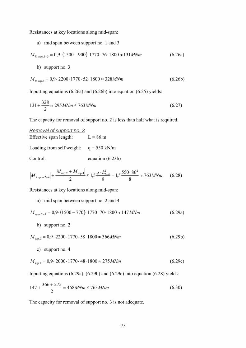
75

Resistances at key locations along mid-span:

a) mid span between support no. 1 and 3

( ) MNmM spanR 131180076177090015009,031.. ≈⋅⋅⋅−⋅=− (6.26a)

b) support no. 3

MNmM R 328180052177022009,03.sup. ≈⋅⋅⋅⋅= (6.26b)

Inputting equations (6.26a) and (6.26b) into equation (6.25) yields:

MNmMNm 7632952

328131 ≤≈+ (6.27)

The capacity for removal of support no. 2 is less than half what is required.

Removal of support no. 3 Effective span length: L = 86 m

Loading from self weight: q = 550 kN/m

Control: equation (6.23b)

MNmLqMMM spanR 763

8865505,1

85,1

2

22424.sup2.sup

42.. ≈⋅

=⋅

≤+

+ −− (6.28)

Resistances at key locations along mid-span:

a) mid span between support no. 2 and 4

( ) MNmM span 147180070177077015009,042. ≈⋅⋅⋅−⋅=− (6.29a)

b) support no. 2

MNmM 366180058177022009,02.sup ≈⋅⋅⋅⋅= (6.29b)

c) support no. 4

MNmM 275180048177020009,04.sup ≈⋅⋅⋅⋅= (6.29c)

Inputting equations (6.29a), (6.29b) and (6.29c) into equation (6.28) yields:

MNmMNm 7634682

275366147 ≤=+

+ (6.30)

The capacity for removal of support no. 3 is not adequate.

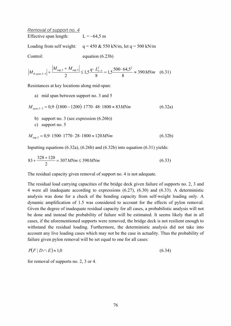
76

Removal of support no. 4 Effective span length: L = ~64,5 m

Loading from self weight: q = 450 & 550 kN/m, let q = 500 kN/m

Control: equation (6.23b)

MNmLqMMM spanR 390

85,645005,1

85,1

2

22535.sup3.sup

53.. ≈⋅

=⋅

≤+

+ −− (6.31)

Resistances at key locations along mid-span:

a) mid span between support no. 3 and 5

( ) MNmM span 831800481770120018009,053. ≈⋅⋅⋅−⋅=− (6.32a)

b) support no. 3 (see expression (6.26b)) c) support no. 5

MNmM 120180028177015009,05.sup ≈⋅⋅⋅⋅= (6.32b)

Inputting equations (6.32a), (6.26b) and (6.32b) into equation (6.31) yields:

MNmMNm 3903072

12032883 ≤=+

+ (6.33)

The residual capacity given removal of support no. 4 is not adequate.

The residual load carrying capacities of the bridge deck given failure of supports no. 2, 3 and 4 were all inadequate according to expressions (6.27), (6.30) and (6.33). A deterministic analysis was done for a check of the bending capacity from self-weight loading only. A dynamic amplification of 1.5 was considered to account for the effects of pylon removal. Given the degree of inadequate residual capacity for all cases, a probabilistic analysis will not be done and instead the probability of failure will be estimated. It seems likely that in all cases, if the aforementioned supports were removed, the bridge deck is not resilient enough to withstand the residual loading. Furthermore, the deterministic analysis did not take into account any live loading cases which may not be the case in actuality. Thus the probability of failure given pylon removal will be set equal to one for all cases:

( ) 0,1| ≈∩ EDFP (6.34)

for removal of supports no. 2, 3 or 4.

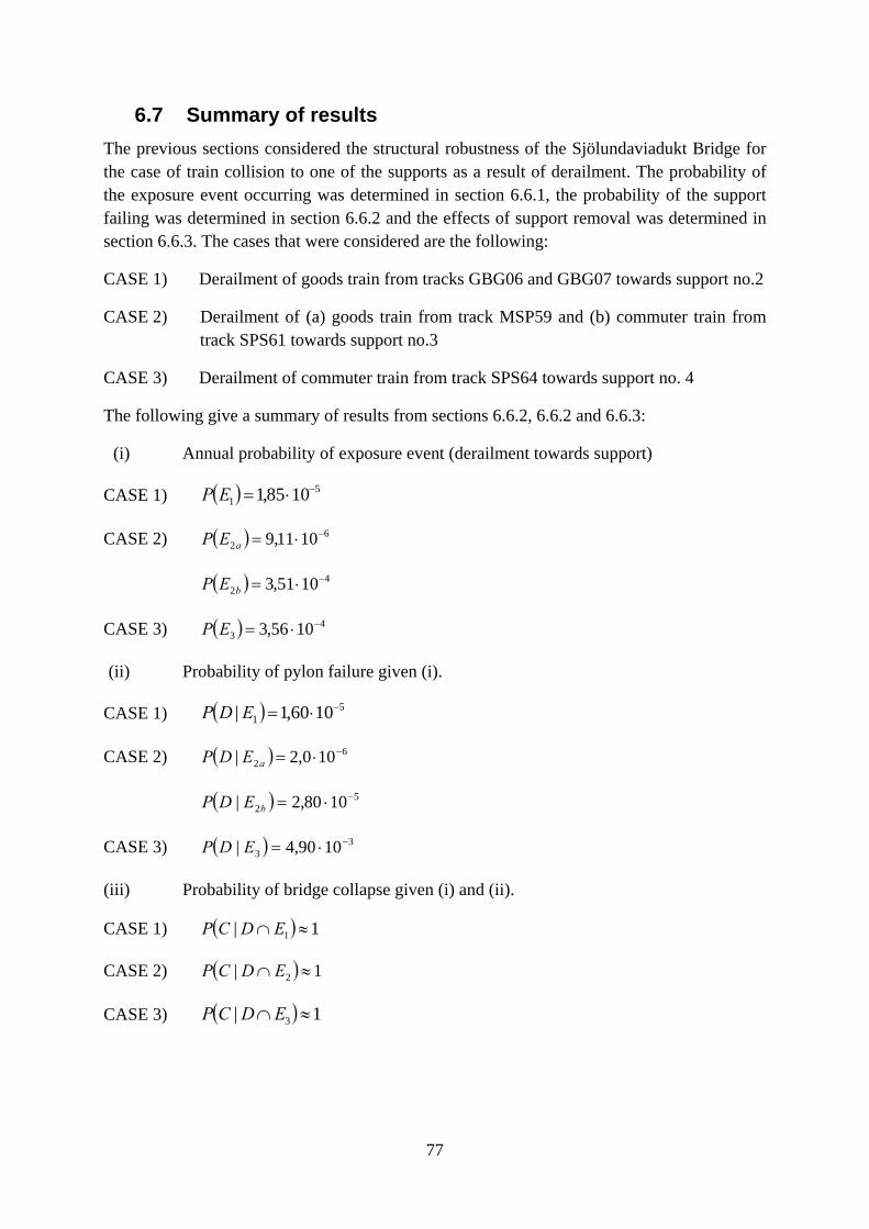
77

6.7 Summary of results The previous sections considered the structural robustness of the Sjölundaviadukt Bridge for the case of train collision to one of the supports as a result of derailment. The probability of the exposure event occurring was determined in section 6.6.1, the probability of the support failing was determined in section 6.6.2 and the effects of support removal was determined in section 6.6.3. The cases that were considered are the following:

CASE 1) Derailment of goods train from tracks GBG06 and GBG07 towards support no.2

CASE 2) Derailment of (a) goods train from track MSP59 and (b) commuter train from track SPS61 towards support no.3

CASE 3) Derailment of commuter train from track SPS64 towards support no. 4

The following give a summary of results from sections 6.6.2, 6.6.2 and 6.6.3:

(i) Annual probability of exposure event (derailment towards support)

CASE 1) ( ) 51 1085,1 −⋅=EP

CASE 2) ( ) 62 1011,9 −⋅=aEP

( ) 42 1051,3 −⋅=bEP

CASE 3) ( ) 43 1056,3 −⋅=EP

(ii) Probability of pylon failure given (i).

CASE 1) ( ) 51 1060,1| −⋅=EDP

CASE 2) ( ) 62 100,2| −⋅=aEDP

( ) 52 1080,2| −⋅=bEDP

CASE 3) ( ) 33 1090,4| −⋅=EDP

(iii) Probability of bridge collapse given (i) and (ii).

CASE 1) ( ) 1| 1 ≈∩ EDCP

CASE 2) ( ) 1| 2 ≈∩ EDCP

CASE 3) ( ) 1| 3 ≈∩EDCP

78

The total probability of collapse is determined from equation (6.1).

( ) ( ) ( ) ( )∑∑ ∩=i j

iijij EPEDPEDFPCP ||

( ) [ ]43

456655

1065,31090,411051,31080,21011,9100,211085,11060,11

−−

−−−−−−

⋅⋅⋅⋅+

⋅⋅⋅+⋅⋅⋅⋅+⋅⋅⋅⋅=CP

( ) [ ] 6691110 1080,11079,11083,91082,11096,2 −−−−− ⋅=⋅+⋅+⋅+⋅=CP (6.35)

The annual probability of failure of the Sjölundaviadukt Bridge due to collisions from derailed trains is 61080,1 −⋅ . This value corresponds to a reliability index (equation 4.1) of:

( ) 63,41080,1 611 =⋅Φ−= −−β (6.36)

for a reference period of one year, and

( ) 75,3501080,1 6150 =⋅⋅Φ−= −−β (6.37)

for a reference period of 50 years

These values correspond to reliability class RC1 (which prescribes the following minimum values: β1 > 4,2 and β50 > 3,3) and consequently consequence class CC1 according to Eurocode (see table 4.1 in section 4.1). The consequence class CC1 is a criterion reserved for structures with low consequences as a result of system malfunction or impairment; a class to which bridge structures should not adhere. The consequence of system malfunction for a bridge is high and the target reliability class should be set to at least RC2. It is thus unusual that given such a rare exposure event, the reliability index for system failure is so low. To help increase the structures integrity towards extraordinary or unknown events, such as train collision, design methods and strategies of robustness need to be considered.

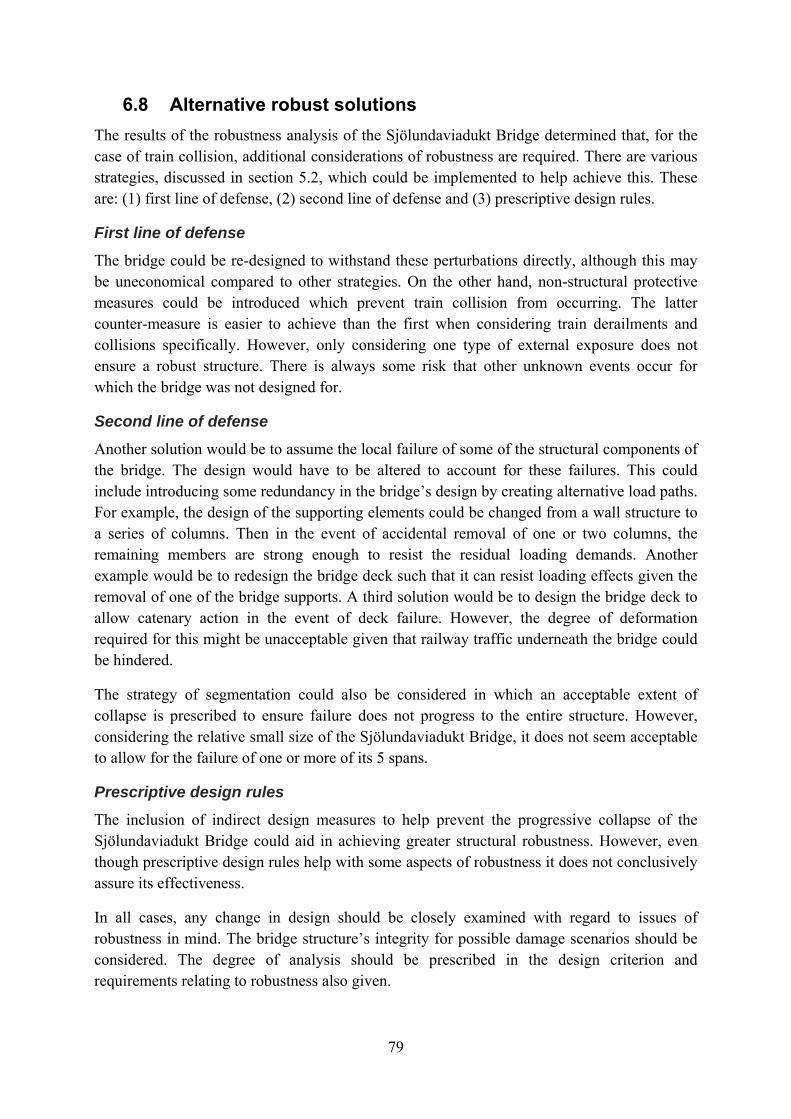
79

6.8 Alternative robust solutions The results of the robustness analysis of the Sjölundaviadukt Bridge determined that, for the case of train collision, additional considerations of robustness are required. There are various strategies, discussed in section 5.2, which could be implemented to help achieve this. These are: (1) first line of defense, (2) second line of defense and (3) prescriptive design rules.

First line of defense The bridge could be re-designed to withstand these perturbations directly, although this may be uneconomical compared to other strategies. On the other hand, non-structural protective measures could be introduced which prevent train collision from occurring. The latter counter-measure is easier to achieve than the first when considering train derailments and collisions specifically. However, only considering one type of external exposure does not ensure a robust structure. There is always some risk that other unknown events occur for which the bridge was not designed for.

Second line of defense Another solution would be to assume the local failure of some of the structural components of the bridge. The design would have to be altered to account for these failures. This could include introducing some redundancy in the bridge’s design by creating alternative load paths. For example, the design of the supporting elements could be changed from a wall structure to a series of columns. Then in the event of accidental removal of one or two columns, the remaining members are strong enough to resist the residual loading demands. Another example would be to redesign the bridge deck such that it can resist loading effects given the removal of one of the bridge supports. A third solution would be to design the bridge deck to allow catenary action in the event of deck failure. However, the degree of deformation required for this might be unacceptable given that railway traffic underneath the bridge could be hindered.

The strategy of segmentation could also be considered in which an acceptable extent of collapse is prescribed to ensure failure does not progress to the entire structure. However, considering the relative small size of the Sjölundaviadukt Bridge, it does not seem acceptable to allow for the failure of one or more of its 5 spans.

Prescriptive design rules The inclusion of indirect design measures to help prevent the progressive collapse of the Sjölundaviadukt Bridge could aid in achieving greater structural robustness. However, even though prescriptive design rules help with some aspects of robustness it does not conclusively assure its effectiveness.

In all cases, any change in design should be closely examined with regard to issues of robustness in mind. The bridge structure’s integrity for possible damage scenarios should be considered. The degree of analysis should be prescribed in the design criterion and requirements relating to robustness also given.

80

81

7. Conclusions and Discussion

The property of structural robustness for bridge systems was investigated and a robustness analysis of the Sjölundaviadukt Bridge conducted. The prior portion of the report addressed the importance of incorporating robustness in the design, construction and maintenance of bridge structures. The latter portion of the report investigated the robustness of the Sjölundaviadukt Bridge with regard to a specified hazard scenario: pylon collision from derailed trains. The objective of the report was to aid the reader in achieving a better understanding of the issues related to bridge robustness and provide an example that accounts for structural robustness considerations for a specified bridge structure.

It is difficult to attempt at a prescribed design procedure which can be used to ensure structural robustness of arbitrary bridge structures. Each bridge should therefore be investigated on a case by case basis and specific design requirement for the robustness of the structure should be given. However, it is also difficult to determine these requirements explicitly and thus far no universally accepted measure of robustness has been developed. Thus it seems that when considering the structural robustness of bridge structures, much interpretation is required in order to attain any conclusive result. There are, however, various strategies and methods that have been developed to help increase the robustness of structures.

Current design procedures were determined to be decisively inadequate with regard to considerations of structural robustness. A framework for the assessment of structural robustness of bridges requires additional methods of analysis to complement current design procedures. While reliability based design focuses on component based analysis and localized effects of hazard events, a systems approach is required which takes into account the consequences of localized damages for the bridge system as a whole. In cases where unknown perturbations must be considered, methods of analysis including investigation of the damage itself rather than its cause have been developed in an effort to account for these actions. However, if extraordinary exposures can be identified, an analysis may be done to determine a measure of robustness for the given event. A risk-consequence analysis is one way of achieving this in which individual perturbations and their associated risks are quantified and the proportionality of impaired function to the initiating cause may be identified.

The robustness analysis of the Sjölundaviadukt Bridge was conducted for the case of pylon collision given derailment of a train. The results of the analysis yielded a marginal annual failure probability of 61080,1 −⋅ . This value determined a reliability and consequence class below that which would be expected for a bridge structure. The bridge itself was designed according to conventional design procedures and included considerations of accidental loading including, specifically, train collision. Despite of this, considerations of robustness in the design of the bridge were not evident. Alternative bridge solutions were briefly discussed which could help in attaining a more robust structure.

82

83

8. References

Literature

Agarwal, J.; Blockley, D.I.; Woodman, N.J. (2003). “Vulnerability of structural systems.” Structural Safety, Vol. 25, pp. 263-286.

Baker, J.W.; Schubert, M.; Faber, M.H. (2006). “On the assessment of robustness.” Structural Safety, Vol. 30, pp. 253-267.

Brabie, D.; Andersson, E. (2007). “Post-derailment dynamic simulation of rail vehicles – methodology and applications.” Vehicle System Dynamics. Vol. 46, Supplement, 2008, 289-300.

Carlsson, F. (2002). “Reliability Based Assessment of Bridges with Short Spans.” Licentiate Thesis. Lund Institute of Technology. Department of Structural Engineering. Report TVBK-1025. Lund 2002.

Champris, D.C. (2008). “Implementation aspects of a robustness index.” Workshop paper, JCSS and IABSE Workshop on Robustness of Structures, Building Research Establishment, Garston, Timisoara, Romania, September 29-30, 2008.

Ellingwood, B.R. (2001). “Acceptable risk bases for design of structures.” Prog. Struct. Engng. Mater., 3, pp. 170-179.

EN 1990:2002. Eurocode-Basis of Structural Design. CEN, 2002.

prEN 1991-7:2003. Eurocode 1: Actions on Structures: Part 1-7: General actions - Accidental Actions. CEN, March 5, 2003. Final project team draft (stage 34).

Fredén, S. (2001). “Modell för skattning av sannolikheten för järnvägsolyckor som drabbar omgivningen.” Banverket. Miljösektionen. Rapport 2001:5. 2001-10-22.

Galambos, T.V. (2008). “The safety of bridges.” NAE, The Bridge, Vol. 32 (2), pp. 20-25.

Grimm, M., Wahlborg, M. (2009). “Kapacitetssituationen 2009 – Banverkets järn-vägsnät.” Banverket. Leveransdivisionen. Rapport 2009-03-31.

Gulvanessian, H.; Vrouwendvelder, T. (2006). “Robustness and the Eurocodes.” Structural Engineering International, 16(2), pp. 167-171.

Joint Committee on Structural Safety - JCSS (2008). Risk Assessment in Engineering – Principles, System Representation & Risk Criteria. June, 2008.

Joint Committee on Structural Safety - JCSS (2001). Probabilistic Model Code. Parts 1,2 & 3. March, 2001.

Knoll, F.; Vogel, T. (2009). Design for Robustness; Structural Engineering Documents No. 11. 2009, IABSE Zurich.

84

Lind, N.C. (1995). “A measure of vulnerability and damage tolerance.” Reliability Engineering and System Safety, 48(1), pp. 1-6.

Maes, M.A.; Fritzsons, K.E.; Glowienka, S. (2006). ”Structural Robustness in the Light of Risk and Consequence Analysis.” Structural Engineering International, 16(2), pp. 101-107.

Melchers, R.E. (1999). Structural Reliability Analysis and Prediction. 2nd ed. John Wiley & Sons Ltd., Chichester, England.

Nowak, A.S.; Collins, K.R. (2000). Reliability of Structures. Internatinoal Ed. McGraw-Hill Companies, Inc., Singapore.

Ratay, R.T. (2007). “Forensic Structural Engineering-Focus on the United States.” Structural Engineering International, 17(2), pp. 114-118.

Ropohl, G. (2009). Eine Systemtheorie der Technik – Zur Grundlegung de allgemeinen Technologie. Carl Hanser Verlag, München Wein 1979.

Schubert, M., Faber, M.H. (2007). “Robustness of Infrastructures subject to rare events.” 10th International Conference on Applications of Statistics and Probability in Civil Engineering, Tokyo, Japan, July 31 – August 03.

Sheer, J. (2000). Versagen von Bauwerken; Band 1: Brücken. Ernst & Sohn, Berlin, Germany.

Smith, J.W. (2006). “Structural Robustness Analysis and the Fast Fracture Analogy.” Structural Engineering International, 16(2), pp. 118-123.

Sparre, E. (1995). “Urspårningar, kollisioner och brander på svenska järnvägar mellan åren 1985 och 1995.” Department of Mathematical Statistics, Lund University. 1995:E9.

Starossek, U. (2006). “Progressive collapse of bridges – Aspects of analysis and design.” Invited lecture, Proceedings, International Symposium on Sea-Crossing Long-Span Bridges, Mokpo, Korea, February 15-17, 2006.

Starossek, U.; Haberland, M. (2008). "Measures of structural robustness – Requirements & applications." Proceedings, ASCE SEI 2008 Structures Congress – Crossing Borders, Vancouver, Canada, April 24-26, 2008.

Starossek, U. (2009). Progressive collapse of structures. Thomas Telford Publishing, London, July 2009.

Stempfle, H.; Vogel, T. (2005). “A concept to evaluate the robustness of bridges.” Workshop paper, JCSS and IABSE Workshop on Robustness of Structures, Building Research Establishment, Garston, Watford, UK, November 28-29, 2005.

Sørensen, J.D.; Christensen, H.H. (2006). “Danish Requirements for Robustness of Structures: Background and Implementation.” Structural Engineering International, 16(2), pp. 172-177.

85

Teknisk Ståbi. 18. Udgave. Nyt Teknisk Forlag, Copenhagen, Denmark. 2004.

Vrouwenvelder, T.; Sørensen, J.D. (2009). ”Robustness of structures, EU COST action TU0601.” Safety, Reliability and Risk of Structures, Infrastructures and Engineering Systems: Proceedings of the tenth International Conference on Structural Safety and Reliability (ICOSSAR2009), Osaka, Japan, 13-17 September

Vägverket. Vägverkets allmänna tekniska beskrivning för nybyggande och förbättring av broar. Bro 2004. Publication 2004:56. Borlänge, Sweden, 2004.

Wardhana, K.; Hadipriono, F.C. (2003). “Analysis of Recent Bridge Failures in the United States.” Journal of Performance of Constructed Facilities, Vol. 17, No. 3, August 2003.

Wisniewski, D.; Casas, J.R.; Ghosn, M. (2006). “Load capacity evaluation of existing railway bridges base on robustness quantification.” Structural Engineering International, 16(2), pp. 161-166.

Östlund, L.; Svensson, S.; Thelandersson, S. (1995). “Dubbelspårsutbyggnad Kävlinge-Lund – Konsekvenser och skyddsåtgärder vid urspårning eller collision.” Lund Institute of Technology. Department of Structural Engineering. Report TVBK-7048.

Åkesson, B. (2008). Understanding Bridge Collapses. Taylor & Francis Group, London, UK.

Internet Sources

[1] Kármán, Theodore von. “Collapse of the Tacoma Narrows Bridge” http://www.ias.ac.in/resonance/Aug2005/pdf/Aug2005Classics.pdf

[2] Robustness of Structures: COST Action TU0601. http://www.cost-tu0601.ethz.ch

[3] COST: European Cooperation in Science and Technology. TUD Action TU0601. http://www.cost.esf.org/domains_actions/tud/Actions/Robustness_of_Structures

[4] Sydsvenskan.se. ”Risk för att Sjölunadviadukten rasar”. Feb. 2008 http://sydsvenskan.se/malmo/article298490/Risk-att-Sjolundaviadukten-rasar.html

[5] http://kartor.eniro.se/ [6] http://webbkameror.se/webbkameror/malmo/malmo_stockholmsv_s_1280.php [7] Banverket. Projekt – Malmö Stad: Sjölundaviadukten

http://www.banverket.se/sv/Amnen/Aktuella-projekt/Projekt/1871/Malmo-stad-Sjolundaviadukten.aspx

Computer programs

[A] MATLAB R2008b (Ver. 7.7.0.471), The MathWorks

[B] AutoCAD 2007, Autodesk

86

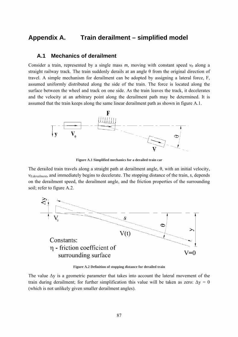
87

Appendix A. Train derailment – simplified model

A.1 Mechanics of derailment Consider a train, represented by a single mass m, moving with constant speed v0 along a straight railway track. The train suddenly derails at an angle θ from the original direction of travel. A simple mechanism for derailment can be adopted by assigning a lateral force, F, assumed uniformly distributed along the side of the train. The force is located along the surface between the wheel and track on one side. As the train leaves the track, it decelerates and the velocity at an arbitrary point along the derailment path may be determined. It is assumed that the train keeps along the same linear derailment path as shown in figure A.1.

Figure A.1 Simplified mechanics for a derailed train car

The derailed train travels along a straight path at derailment angle, θ, with an initial velocity, v0.derailment, and immediately begins to decelerate. The stopping distance of the train, s, depends on the derailment speed, the derailment angle, and the friction properties of the surrounding soil; refer to figure A.2.

Figure A.2 Definition of stopping distance for derailed train

The value Δy is a geometric parameter that takes into account the lateral movement of the train during derailment; for further simplification this value will be taken as zero: Δy = 0 (which is not unlikely given smaller derailment angles).

88

The stopping distance of a derailed train can be determined for a given derailment speed, v0.derailment. A simplification is introduced which assumes that the initial velocity after derailment may be taken as the velocity of the train just as derailment occurs:

v0.derailment = v0

As the train travels along an angle θ on the surrounding soil, it decelerates due to a friction force gmR ⋅⋅=η . The force exerted by the train as it decelerates (at any given time, t) must be equal to the reacting friction force R (the energy loss to other forms such as sound and heat is neglected):

( ) gmR

dtdvR

dtdvmtF ⋅−=−=⇒−=⋅= η

(A.1)

Thus the speed after time t is:

( ) tgvtv ⋅⋅−= η0 (A.2)

The time needed for the train to stop is then found (i.e. t for v(t) = 0):

( ) gvttv ss η/0 0=→= (A.3)

The stopping distance, s, is the integral of velocity from equation (A.2) over the time it takes the train to come to rest, ts:

2

2

0s

stgtvs ⋅⋅−⋅= η

(A.4)

inserting equation (A.3) into (A.4) yields

gvsη2

20=

(A.5)

A.1.1 Velocity at impact The velocity at impact for a derailed train will be determined. Equation (A.5) may be rewritten such that the stopping distance, s, is set to the distance from the point of derailment to a support, sobs, for a given derailment angle θ. Then the time needed for the train to collide with the support is obtained.

obsobsobsobs

obsobs stvtgtgtvs −⋅+⋅⋅

−=⇒⋅⋅−⋅= 02

2

0 20

2ηη

gsgv

gvt obs

obs ηη

η⋅⋅−

−=22

00 (A.6)

89

Inserting equation (A.6) into equation (A.2) yields the velocity at impact:

( ) obsimpobsobsimp sgvvtgvtvv ⋅⋅−=⇒⋅⋅−== ηη 2200

θη

sin22

0obs

impygvv ⋅⋅−= (A.7)

A.1.2 Force at impact The velocity of a derailed train when it collides with a column can be determined from expression (A.7), the corresponding impact force, Fimp, from the train may be evaluated. There are various methods for determining this force including kinematic and stiffness relations. Here two separate simplified methods for determining Fimp are considered: (1) impulse momentum equilibrium and (2) energy equilibrium. It will be assumed that the pylon is a rigid body and thus only the properties of the derailed train will be considered.

The aforementioned methods for determining Fimp are based the following relationships:

(1) The change in momentum that a body undergoes during collision is equal to the collision force times the impulse time, Δt (duration of collision):

tFvm impimp Δ⋅=⋅

tvm

F impimp Δ

⋅=⇒ (A.8a)

(2) The work done by a body during a collision is equal to the kinetic energy generated at impact:

2

2imp

imp

vmsF

⋅=Δ⋅

s

vmF imp

imp Δ⋅⋅

=⇒2

2

(A.8b)

Δs the distance in which the center of gravity of the body travels during collision; i.e. the “shortening” distance of the train in this case.

Since neither Δt nor Δs can be explicitly determined, suitable estimations will need to be made.

90

A.2 Maximum derailment angle, θmax The tendency is for the train to rotate about its primary axis and possibly topple (roll) over during derailment. This is due to a reaction force from the mechanism of derailment, located at the contact point between the wheel and rail. This force lies below the center of gravity for the rail car and toppling becomes possible. If the train were to roll on its side during derailment its movement becomes more restrictive. Östlund et. al (1995) determined that a maximum derailment angle, θmax, for a given initial train speed, v0, determined whether or not the train would topple. The following inverse relationship between the derailment angle and derailment speed was found:

mradCwhere

vC sec.5,3,

0max =≈θ (A.10)

The above relation was determined based on the possible toppling of a locomotive engine but will be adopted to apply for goods- and passenger-trains for the purposes of simplification

Figure A.3 is a graph showing the relationship between the derailment velocity and maximum derailment angle given in equation (A.10).

Figure A.3 Maximum derailment angle plotted against derailment velocity

0

2

4

6

8

10

12

14

16

18

20

0 10 20 30 40 50 60

Maxim

um derailm

ent a

ngle, θ

max[°]

Derailment velocity, v0 [m/s]

91

A.2.1 Statistical parameters for θmax The maximum derailment angle from equation (A.10) is linearly dependent of a variable C and inversely proportional to the initial speed at derailment v0. The prior will be assumed a random variable with a lognormal distribution with the following mean value, coefficient of variation and standard deviation (Östlund et al. 1995):

msradVV

msrad

CCCCC⋅

==⇒=⋅

= 75,15,05,3 μσμ (A.11)

The derailment velocity v0 is also a random variable and it will be assumed that is follows a lognormal distribution. The mean value may be taken as the specified speed limit for the region of track being considered and a reasonable amount of variation will be assumed:

000001,0. vvvvv VVvaluenom μσμ === (A.12)

Thus the maximum yaw angle is a product of two lognormal random variables that are assumed statistically independent. By taking the natural logarithm of equation (A.10) we get:

0max lnlnln vC −=θ (A.13)

This equation represents a sum of normally distributed random variables ln(C) and ln(v0) and thus ln(θmax) is also normally distributed. Which, by definition, means that θmax is a lognormally distributed random variable with the following mean and standard deviation (Nowak et al. 2000):

0max lnlnln vC μμμ θ −= (A.14a)

2ln

2ln

2ln 0max vC σσσ θ += (A.14b)

where

( )22ln 1ln

ii XX V+=σ (A.14c)

( ) 2lnln 2

1lniii XXX σμμ −= (A.14d)

The corresponding distribution parameters of the lognormally distributed variable θmax are then calculated by rewriting equations (A.14c) and (A.14d).

with ( ) ( ) 2lnln

22ln maxmaxmaxmaxmax 2

1ln1ln θθθθθ σμμσ −=+= andV the following is yielded:

12

maxln

max−= θσ

θ eV (A.15a)

92

and

( ) ( ) ( ) ⎥⎦

⎤⎢⎣

⎡+⋅=⎥

⎦

⎤⎢⎣

⎡++=

−−21

221

2ln maxmaxmaxmaxmax

1ln1lnln θθθθθ μμμ VV

( )21

2max

maxln

max1 θ

μθ

θμ Ve +⋅=⇒ (A.15b)

A.3 Minimum derailment angle, θmin The minimum derailment angle will be defined as the angle for which, given derailment, the stopping distance of the train is equivalent to the distance from the derailment point to the impact point; i.e. the train reaches zero velocity just as it approaches the pylon. In order to determine the minimum yaw angle for pylon collision given derailment, the post-derailment behavior of the train must considered.

The formula for the stopping distance of a derailed train is given in equation (A.5). To determine the minimum derailment angle, the stopping distance will be set equal to the distance between the point of derailment and the support: s = sobs. For a given perpendicular distance of an obstruction from the center of the track, yobs, the following minimum derailment angle can then be formulated (refer to figure A.2 and figure 6.11):

( )obs

obsobsobs s

yyyys Δ+=→Δ+= −1

minmin sinsin/ θθ (A.16)

Inputting equation (A.5) into equation (A.16) and letting Δy = 0, the minimum yaw angle becomes:

20

11min

2sinsinv

gysy obs

obs

obs ⋅⋅== −− ηθ (A.17)

A.3.1 Statistical parameters for θmin The minimum derailment angle from equation (A.17) is dependent on the derailment velocity, v0, the perpendicular distance from the track to the support, yobs, and the friction coefficient of the surrounding soil, η:

• The velocity at derailment, v0, follows a lognormal distribution with a coefficient of variation given in expression (A.3).

• The perpendicular distance from the rail tracks to the support, yobs, is assumed deterministic and depends on which support is being analyzed.

• The friction coefficient of the surround soil, η, will be modeled as a random variable with a lognormal distribution.

93

Friction coefficient η

The friction coefficient is hard to determine without more detailed empirical investigation of the site. It is dependent on the surface properties of the soil including climactic influences such as frost or dampness. Figure A.4 shows various values for θmin given different friction coefficients, η, for derailment of a train towards support no.2.

Figure A.4 Minimum derailment angle vs. derailment velocity for support no. 2 (yobs = 3m) given varying soil friction coefficients

The mean value for η will be assumed at 0,5 and considering the degree of uncertainty to its actual value, a relatively large coefficient of variation will be assumed (Östlund et. al 1995):

25,05,05,0 ==⇒== ηηηηη μσμ VV (A.18)

The statistical properties of the minimum yaw angle, θmin, can now be determined.

The following simplification can be made to equation (A.17):

(from first order Taylor series for f(x) = sin-1 x ≈ x):

gyKwherev

Kofvaluessmallforv

gyv

gyobs

obsobs 222sin 120

120

20

1min =⋅≈= − ηηηθ (A.19)

NOTE: from Figure A.5 it can be seen that the first order Taylor approximation from eq. (A.19) is acceptable for ca. θmin < 20 deg. This seems a reasonable approximation.

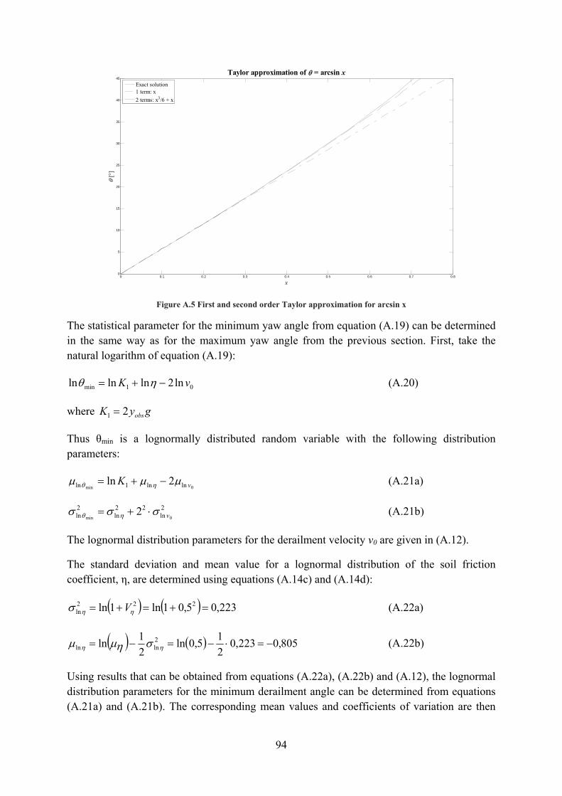
94

Figure A.5 First and second order Taylor approximation for arcsin x

The statistical parameter for the minimum yaw angle from equation (A.19) can be determined in the same way as for the maximum yaw angle from the previous section. First, take the natural logarithm of equation (A.19):

01min ln2lnlnln vK −+= ηθ (A.20)

where gyK obs21 =

Thus θmin is a lognormally distributed random variable with the following distribution parameters:

0min lnln1ln 2ln vK μμμ ηθ −+= (A.21a)

2ln

22ln

2ln 0min

2 vσσσ ηθ ⋅+= (A.21b)

The lognormal distribution parameters for the derailment velocity v0 are given in (A.12).

The standard deviation and mean value for a lognormal distribution of the soil friction coefficient, η, are determined using equations (A.14c) and (A.14d):

( ) ( ) 223,05,01ln1ln 222ln =+=+= ηησ V (A.22a)

( ) ( ) 805,0223,0215,0ln

21ln 2

lnln −=⋅−=−= ηη σημμ (A.22b)

Using results that can be obtained from equations (A.22a), (A.22b) and (A.12), the lognormal distribution parameters for the minimum derailment angle can be determined from equations (A.21a) and (A.21b). The corresponding mean values and coefficients of variation are then

0 0.1 0.2 0.3 0.4 0.5 0.6 0.7 0.80

5

10

15

20

25

30

35

40

45Taylor approximation of θ = arcsin x

x

θ [°

]

Exact solution1 term: x2 terms: x3/6 + x

95

obtained analogously as for the maximum derailment angle (refer to equations (A.15a) and (A.15b)).

12

minln

min−= θσ

θ eV (A.23a)

( )21

2min

minln

min1 θ

μθ

θμ Ve +⋅= (A.23b)

A.4 Critical region for derailment, xcrit Now that the maximum and minimum derailment angles have been determined, the critical distance defined in equation (6.3) can be obtained. Equation (6.3) can be simplified by substituting the first order Taylor approximation for f(x) = 1/tan x ≈ 1/x (refer to Figure A.6):

( ) ( ) maxminmaxmin tantan θθθθobsobsobs

obsobsobsobs

obscritybyLybyLx −

++≈−

++= (A.24)

Figure A.6 First and second order Taylor approximations for cotan θ

A.4.1 Statistical parameters for xcrit Equation (A.24) is a nonlinear function of two random variables, both of which adhere to lognormal distributions. To solve this type of function a linearization can be performed using a first order Taylor series expansion of the random variable function, Y = f(θmin, θmax) = xcrit, and then estimating the mean and variance of the linearized function (Nowak et al. 2000). The “design point values” used for this determination are the mean values of the random variables θmin and θmax; i.e.

minθμ and maxθμ .

( )maxmin

maxmin,θθ

θθ obsobsobsobs

ybyLfY −+

+== (A.25b)

0 5 10 15 20 25 30 35 40 450

2

4

6

8

10

12

14

16

18

20Taylor approximation of cotan θ

θ [°]

cota

n θ

Exact solution1 term: 1/x2 terms: 1/x - x/3

96

then

( ) ( )( )

( )( )maxmin

max

maxmin

minmaxmin

,maxmax

,minmin,

θθθθ μμθ

μμθθθ θ

μθθ

μθμμ∂∂

⋅−+∂∂

⋅−+≈fffY (A.25b)

The evaluation of the first order partial derivatives at the design points yields:

( )( )

( )2

,min2minmin minmaxmin

θμμμθθθ

θθ

obsobsobsobs byfbyf +−=

∂∂

⇒+−

=∂∂ (A.26a)

( )2

,max2maxmax maxmaxmin

θμμμθθθ

θθ

obsobs yfyf=

∂∂

⇒=∂∂ (A.26b)

Substituting these values into the linearized equation (A.25b) and plugging in the mean values of the variables gives the following form of Y:

( ) ( ) 2max2minmax

max

min

min

maxmin θθ

θθ

θθ μμθ

μμθ

μμobsobsobsobsobsobs

obsybyybyLY ⋅−+

+⋅−−−

++=

(A.27)

This will yield an equation in the following form:

max2min10 θθ ⋅+⋅+= AAAY (A.28)

This is now a linear function of random variables in which the mean and variance of Y can be obtained:

maxmin 210 θθ μμμμ ⋅+⋅+=≈ AAAYxcrit (A.29a)

222

221

22maxmin θθ σσσσ ⋅+⋅=≈ AAYxcrit

(A.29b)

with crit

crit

critx

xxV

μσ 2

=

where

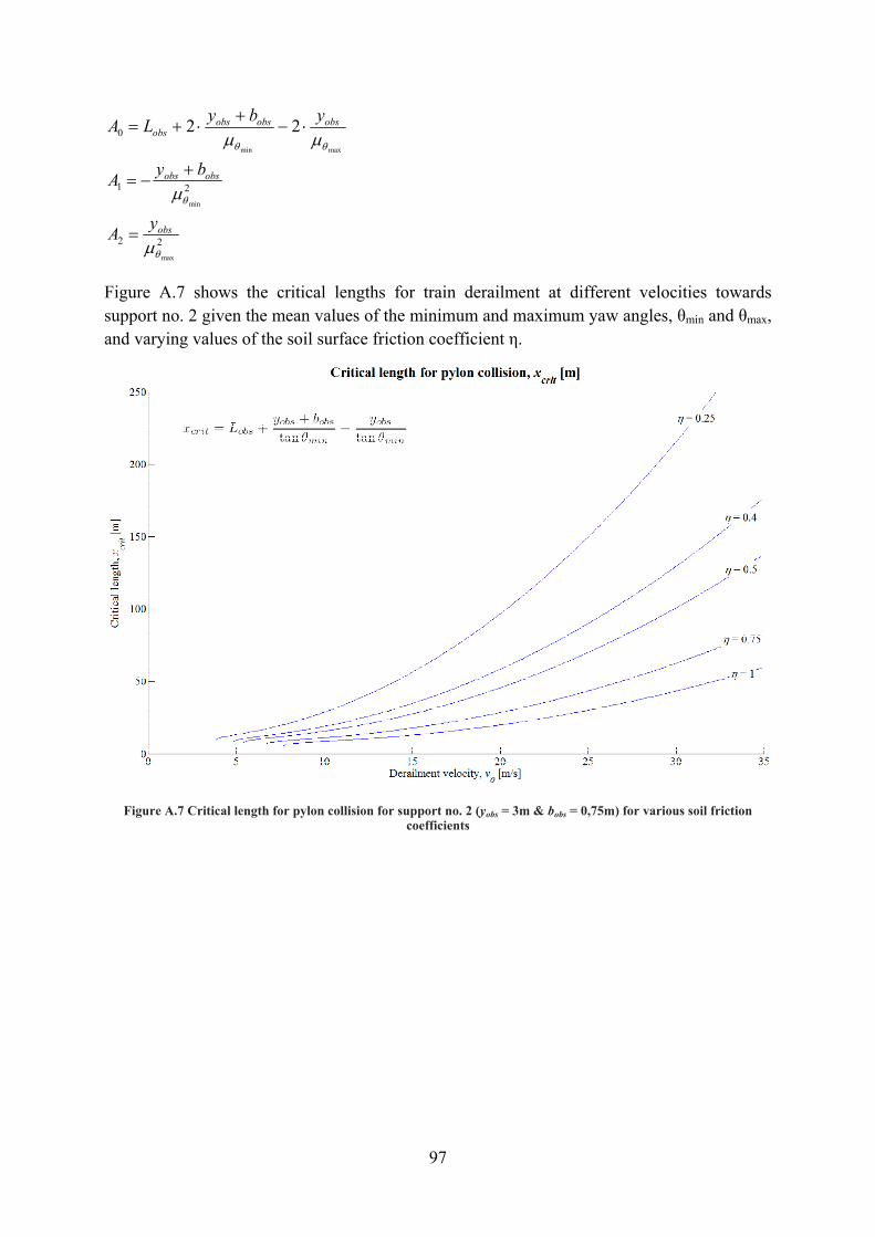
97

22

21

0

max

min

maxmin

22

θ

θ

θθ

μ

μ

μμ

obs

obsobs

obsobsobsobs

yA

byA

ybyLA

=

+−=

⋅−+

⋅+=

Figure A.7 shows the critical lengths for train derailment at different velocities towards support no. 2 given the mean values of the minimum and maximum yaw angles, θmin and θmax, and varying values of the soil surface friction coefficient η.

Figure A.7 Critical length for pylon collision for support no. 2 (yobs = 3m & bobs = 0,75m) for various soil friction coefficients

98

99

Appendix B. Probability of derailment

B.1 Model for probability calculations of train accidents in Sweden

The calculation model to determine the probability of train derailment on Swedish railroads (Fredén 2001) takes into account different causes of derailments and determines the expected number of derailments annually attributed to each cause. The expected number of derailments per year due to differing causes is determined by the following simple linear relationship of two variables:

ξϕ ⋅=W (B.1)

where W is the so called exposure variable and ξ the corresponding intensity factor for the relevant causes given in table B.1 from (Fredén 2001).

In this way the total expected number of derailments per year is then obtained as the sum of inter-dependent linear functions.

∑ ⋅=i

iiWP ξ0

(B.2)

There are two types of tracks that can be considered, those designated for goods trains and those designated for passenger trains. The probability of derailment is not the same for these situations and must be calculated separately. Refer to section B.2 for calculation of derailment for an arbitrary track length of 1 km for the goods train rails and passenger/commuter train rails in the vicinity of the Sjölundaviadukt Bridge.

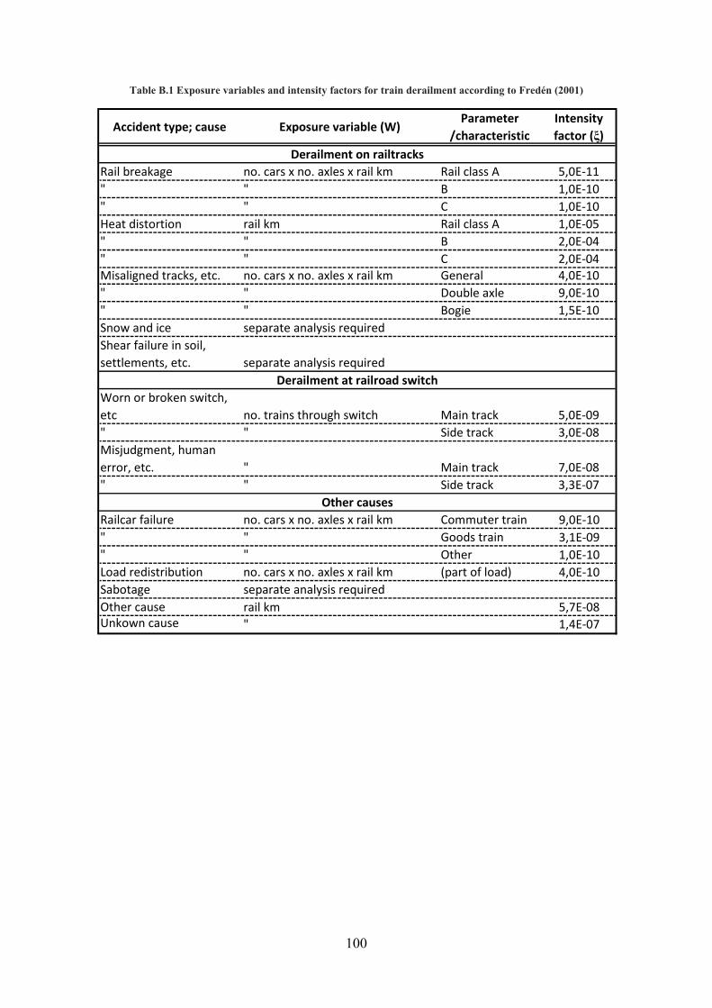
100

Table B.1 Exposure variables and intensity factors for train derailment according to Fredén (2001)

Accident type; cause Exposure variable (W)Parameter 

/characteristicIntensity factor (ξ)

Rail breakage no. cars x no. axles x rail km Rail class A 5,0E‐11" " B 1,0E‐10" " C 1,0E‐10Heat distortion rail km Rail class A 1,0E‐05" " B 2,0E‐04" " C 2,0E‐04Misaligned tracks, etc. no. cars x no. axles x rail km General 4,0E‐10" " Double axle 9,0E‐10" " Bogie 1,5E‐10Snow and ice separate analysis requiredShear failure in soil, settlements, etc. separate analysis required

Worn or broken switch, etc no. trains through switch Main track 5,0E‐09" " Side track 3,0E‐08Misjudgment, human error, etc. " Main track 7,0E‐08" " Side track 3,3E‐07

Railcar failure no. cars x no. axles x rail km Commuter train 9,0E‐10" " Goods train 3,1E‐09" " Other 1,0E‐10Load redistribution no. cars x no. axles x rail km (part of load) 4,0E‐10Sabotage separate analysis requiredOther cause rail km 5,7E‐08Unkown cause " 1,4E‐07

Derailment on railtracks

Derailment at railroad switch

Other causes

101

B.2 Train derailment near Sjölundaviadukt Bridge The railroad tracks running under the Sjölundaviadukt Bridge are either designated for goods train or commuter train traffic and the probability of derailment on these tracks will be determined (a layout of the bridge and tracks is shown in figure 6.5 in section 6.2). In order to quantify the expected number of derailments per year the causes relevant for this case must first be identified; i.e. accident types shown in table B.1. The following lists show the accident types which will be considered as well as those which will be neglected.

Relevant accident types:

Rail breakage Heat distortion Worn or broke switch1 Misjudgment, human error, etc. at railroad switch1 Railcar failure Load redistribution Other cause Unknown cause

Neglected accidental types:

Misaligned tracks, etc. Snow and ice Shear failure in soil, settlements, etc. Sabotage2

1 – depending on the length of the critical region 2 – hard to quantify probability of sabotage The probability of train derailment for an arbitrary track length is calculated for tracks designated for both goods and commuter trains. The direction of traffic is designated for commuter trains on tracks SP61-64 while it will be assumed that tracks designated for goods trains allow for traffic in both directions. The relevant exposure variables that will be used to calculate derailment probabilities are listed above with reference to table B.1. Tables B.2 and B.3 show the calculated probability of derailment, P0 from equation (6.2) is section 6.6.1, for an arbitrary railway length of 1km in the area near the bridge for both goods trains and commuter trains. NOTE: derailment at the railroad switch is neglected.

102

Table B.2 Annual expected number of derailments for goods train tracks near Sjölundaviadukt Bridge; for traffic in both directions and track length = 1km

Table B.3 Annual expected number of derailments for commuter train tracks near Sjölundaviadukt Bridge; for traffic in one direction and track length = 1km

Accident type; causeExposure 

variable (W)Intensity factor (ξ)

Expected no. occurences

Rail breakage 1,37E+06 5,0E‐11 6,86E‐05Heat distortion 1 1,0E‐05 1,00E‐05

Worn or broken switch, etc 0 5,0E‐09 0,00E+00Misjudgment, human error, etc. 0 7,0E‐08 0,00E+00

Railcar failure 1,37E+06 3,1E‐09 4,25E‐03Load redistribution 1,37E+06 4,0E‐10 5,49E‐04Other cause 3,43E+04 5,7E‐08 1,96E‐03Unkown cause 3,43E+04 1,4E‐07 4,80E‐03

Total expected no. occurences per year, P 0 =  1,16E‐02

Other causes

Derailment on railtracks

Derailment at railroad switch

Accident type; causeExposure 

variable (W)Intensity factor (ξ)

Expected no. occurences

Rail breakage 3,39E+05 5,0E‐11 1,70E‐05Heat distortion 1 1,0E‐05 1,00E‐05

Worn or broken switch, etc 0 5,0E‐09 0,00E+00Misjudgment, human error, etc. 0 7,0E‐08 0,00E+00

Railcar failure 3,39E+05 9,0E‐10 3,06E‐04Load redistribution 3,39E+05 4,0E‐10 1,36E‐04Other cause 5,66E+04 5,7E‐08 3,22E‐03Unkown cause 5,66E+04 1,4E‐07 7,92E‐03

Total expected no. occurences per year, P 0 =  1,16E‐02

Derailment on railtracks

Derailment at railroad switch

Other causes

103

Appendix C. Resistance of support wall

C.1 Moment-Normal force graph An arbitrary reinforced concrete cross section with a combined uni-axial moment and normal force action is shown in figure C.1. The neutral axis is defined where the strain in the cross section is equal to zero and its depth from the top edge of the compressed section is denoted by x. An ultimate limit state design is adopted with a plastic rectangular stress distribution as shown in figure C.1.

Figure C.1 Reinforced cross section with combined bending and axial force

A moment-normal force graph can be created which takes into account the combined effect of axial and bending forces. The different values on the graph depend on the depth of the neutral axis as shown in figure C.2. The part of the graph marked balanced reinforcement refers to the condition in which the concrete fails at exactly the same moment as the reinforcement fails; i.e. the strain in concrete is εc = εcu (ultimate strain = 3,5‰) and the strain in reinforcement is εs = εsyd (yield strain = 2,17‰). The part of the graph marked pure bending is for a cross section without any axial force, N, in which the reinforcement yields before the concrete fails; i.e. εc = εcu and εs > εsyd. Thus in both cases, the force in the reinforcement can be determined from equation (C.1)

sys AfF ⋅= (C.1)

where fy is the yield strength of the reinforcing steel.

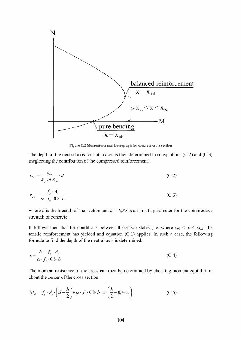
104

Figure C.2 Moment-normal force graph for concrete cross section

The depth of the neutral axis for both cases is then determined from equations (C.2) and (C.3) (neglecting the contribution of the compressed reinforcement).

dxcusyd

cubal ⋅

+=

εεε (C.2)

bfAf

xc

sypb ⋅⋅⋅

⋅=

8,0α (C.3)

where b is the breadth of the section and α = 0,85 is an in-situ parameter for the compressive strength of concrete.

It follows then that for conditions between these two states (i.e. where xpb < x < xbal) the tensile reinforcement has yielded and equation (C.1) applies. In such a case, the following formula to find the depth of the neutral axis is determined:

bfAfN

xc

sy

⋅⋅⋅⋅+

=8,0α

(C.4)

The moment resistance of the cross can then be determined by checking moment equilibrium about the center of the cross section.

⎟⎠⎞

⎜⎝⎛ ⋅−⋅⋅⋅⋅⋅+⎟

⎠⎞

⎜⎝⎛ −⋅⋅= xhxbfhdAfM csyR 4,0

28,0

2α (C.5)

105

Equation (C.5) only applies if the depth of the neutral axis from equation (C.4) is between the values given by expressions (C.2) and (C.3). Table C.1 calculates these values for supports no. 2, 3 and 4 for mean values of fy, fc (refer to table 6.7). Refer to table 6.1 and table 6.6 for the geometry of the support walls including reinforcement.

Table C.1 Calculation of neutral axis depth for supports no. 2, 3 and 4

Equation (C.5) can thus be used to calculate the capacity of all supports.

Support no.

x pb x x bal Check

[mm] [mm] [mm] ‐2 112 198 435 OK3 187 267 528 OK4 93 141 528 OK

106

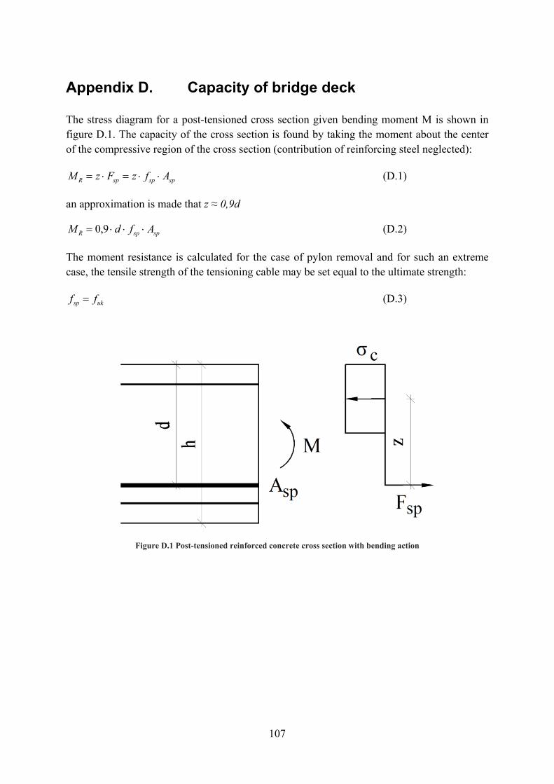
107

Appendix D. Capacity of bridge deck

The stress diagram for a post-tensioned cross section given bending moment M is shown in figure D.1. The capacity of the cross section is found by taking the moment about the center of the compressive region of the cross section (contribution of reinforcing steel neglected):

spspspR AfzFzM ⋅⋅=⋅= (D.1)

an approximation is made that z ≈ 0,9d

spspR AfdM ⋅⋅⋅= 9,0 (D.2)

The moment resistance is calculated for the case of pylon removal and for such an extreme case, the tensile strength of the tensioning cable may be set equal to the ultimate strength:

uksp ff = (D.3)

Figure D.1 Post-tensioned reinforced concrete cross section with bending action