Robust Control - ENCYCLOPEDIA OF LIFE SUPPORT ... – EOLSS SAMPLE CHAPTERS CONTROL SYSTEMS,...

UNESCO – EOLS

S

SAMPLE C

HAPTERS

CONTROL SYSTEMS, ROBOTICS, AND AUTOMATION – Vol. IX – Robust Control - S.P. Bhattacharyya

©Encyclopedia of Life Support Systems (EOLSS)

ROBUST CONTROL S.P.Bhattacharyya Texas A&M University, Texas, USA Keywords: control systems, robust control, optimal control, robust performance, robustness, feedback system, unity feedback, stability, robust stability, servomechanism, tracking, disturbance rejection, stabilization, robustification, stability margin, gain margin, phase margin, H∞ optimal control, l1 optimal control, absolute stability, integral control, PID controller, state space model, state feedback, observers, closed loop eigenvalues, Internal Model Principle, block diagram, characteristic equation. Contents 1. Introduction and Basic Elements of Control Systems 2. Feedback and Robustness 3. Robustness and Integral Control 4. A Short History of Control Theory and Robust Control 4.1. The Classical Period 4.2. Modern Control Theory 4.3. The Servomechanism Problem 4.4. Post-modern Control Theory 4.5. The Parametric Theory 5. Robustness of Control Systems 5.1 Performance Issues and Tradeoffs 5.2. Zero Steady State Errors 6. Feedback Stabilization of Linear Systems 6.1. Stabilization by Observer Based State Feedback 6.2. Pole Placement Compensators 6.3. YJBK Parameterization 6.4. Nyquist Criterion 6.5. Optimal Control: Linear Quadratic Regulator (LQR) 7. Uncertainty Models and Robustness 7.1. Gain and Phase Margin 7.2. Parametric Uncertainty 7.3. Nonparametric and Mixed Uncertainty 8. H∞ Optimal Control 8.1. State Space Theory of H∞ Optimal Control 8.2. Linear Matrix Inequalities 8.3. Frequency Domain Aspects of H∞ Optimal Control 9. µ Theory 10. Quantitative Feedback Theory 11. Concluding Remarks Acknowledgements Glossary Bibliography Biographical Sketch

UNESCO – EOLS

S

SAMPLE C

HAPTERS



Summary Robust control is that branch of control theory which deals explicitly with system uncertainty and how it affects the analysis and design of control systems. In this article, we give an overview of robust control. We begin by describing the fundamental property of robustness inherent in a properly designed feedback structure. First, we show how a feedback system can be used to obtain an accurately controlled gain despite large parameter variability. Then, we demonstrate how integral control in a stable feedback system can precisely zero out the steady state error despite large plant uncertainty. This is followed by a short historical account of control theory and robust control. We then trace the central role robustness has played in classical control designs, linear quadratic optimal control methods, H∞ optimal control techniques, absolute stability methods, and parametric robustness methods. These various approaches develop different analysis and design techniques to address the same basic problem of obtaining precise behavior from physical systems in the presence of significant uncertainty regarding the system models and signals. 1. Introduction and Basic Elements of Control Systems In this section, we make some introductory and motivational remarks describing the problems of robust stability and control. We begin with some basic control concepts, terminology and techniques. This is followed by two sections dealing with the robustness of feedback systems to large parameter variations. Next, a brief historical sketch of control theory is included to serve as a background for the discussion of robustness. This is followed by a description of various uncertainty models in robust control and some of the current techniques for the design of robust control systems. To understand the concept of robustness in the context of control systems it is necessary to begin with a description of the basic functioning of a control system. We do so in the brief overview that follows. Control theory and control engineering deal with dynamic systems such as aircraft, spacecraft, ships, trains and automobiles, chemical and industrial processes such as distillation columns and rolling mills, electrical systems such as motors, generators and power systems, machines such as numerically controlled lathes and robots. In each case, the setting of the control problem is:

1. There are certain dependent variables, called outputs to be controlled, which must be made to behave in a prescribed way. For instance, it may be necessary to assign the temperature and pressure at various points in a process, or the position and velocity of a vehicle, or the voltage and frequency in a power system, to given desired fixed values, despite uncontrolled and unknown variations at other points in the system.

2. Certain independent variables called inputs, such as voltage applied to the motor terminals, or valve position, are available to regulate and control the behaviour of the system. Other dependent variables, such as position, velocity or temperature are accessible as dynamic measurements on the system.

UNESCO – EOLS

S

SAMPLE C

HAPTERS



3. There are unknown and unpredictable disturbances impacting the system. These could be, for example, the fluctuations of load in a power system, disturbances such as wind gusts acting on a vehicle, external weather conditions acting on an air conditioning plant or the fluctuating load torque on an elevator motor, as passengers enter and exit.

4. The equations describing the plant dynamics, and the parameters contained in these equations, are not known at all or at best known imprecisely. This uncertainty can arise, even when the physical laws and equations governing a process are known well, for instance, because these equations were obtained by linearizing a nonlinear system about an operating point. As the operating point changes so do the system parameters.

These considerations suggest the general representation of the plant, or system to be controlled, shown in Figure 1.

The inputs or outputs shown in Figure 1 could actually be representing a vector of signals. In such cases, the plant is said to be a multivariable plant, as opposed to the case, where the signals are scalar, in which case the plant is said to be a scalar or monovariable plant.

Figure 1: A general plant Control is exercised by feedback, which means that the corrective control input to the plant is generated by a device which is driven by the available measurements. Thus the controlled system can be represented by the following feedback or closed loop system shown in Figure 2.

Figure 2: A feedback control system The control design problem is to determine the characteristics of the controller so that

UNESCO – EOLS

S

SAMPLE C

HAPTERS



the controlled outputs can be:

1. Made to closely follow or equal prescribed values called references, which may be constant or time-varying,

2. Maintained at the reference values despite the unknown disturbances, 3. Conditions (1) and (2) are met despite the inherent uncertainties and changes in

the plant dynamic characteristics. The first condition is called tracking, the second, disturbance rejection and the third robustness of the system. The simultaneous satisfaction of (1), (2) and (3) is called robust tracking and disturbance rejection and control systems designed to achieve this are called robust servomechanisms. In the next two sections, we show how the challenging design requirements described here can be met by using properly designed feedback structures. 2. Feedback and Robustness In this section, we illustrate how robust systems can be built from highly unreliable components by using the feedback structure. Specifically, we consider the problem of obtaining a precisely controlled value of gain from a system containing large parameter uncertainty. Consider the system shown in Figure 3. Suppose that the system gain G is required to be 100. Due to poor reliability of the components, this can vary by 50%.

Figure 3: An open loop system Then the actual gain can range from 50 to 150. To remedy this situation, we use the feedback structure shown in Figure 4.

Figure 4: A feedback system

UNESCO – EOLS

S

SAMPLE C

HAPTERS



The gain G is again made with the same unreliable components but with nominal value much higher than 100, say 10,000, and we set C = 0.01. The overall gain of the feedback system is given by the expression

1

GCG+

. (1)

It can easily be verified that with 50% variation in G (that is, G varies from 5,000 to 15,000) the gain of the feedback system varies from 98.039 to 99.338. This remarkable increase in robustness, corresponding to a reduction of uncertainty from 50% to 1%, is one of the main reasons for the widespread use of feedback in the control and electronics industry. In the next section, we illustrate another wonderful application of feedback to the tracking and disturbance rejection problem. 3. Robustness and Integral Control Integral control is used almost universally in the control industry to design robust servomechanisms. It works magically to remove tracking errors in the presence of disturbances even when very little is known regarding the signals and system characteristics. Integral action is most easily implemented by computer control. It turns out that hydraulic, pneumatic, electronic and mechanical integrators are also commonly used elements in control systems. In this section, we explain how integral control works in general to achieve robust tracking and disturbance rejection. Let us first consider an integrator, shown in Figure 5. The input-output relationship is given by

Figure 5: An integrator

( ) ( ) ( )

00

ty t K u d y= τ τ+∫ (2)

or

( )dy Ku t

dt=

(3) where K is the integrator gain. Now suppose that the output y(t) is a constant. It follows from Eq. (3) that

UNESCO – EOLS

S

SAMPLE C

HAPTERS



( )0 0dy Ku t t

dt= = ∀ >

. (4) Equation (4) proves the following important facts about the operation of an integrator:

1. If the output of an integrator is constant over a segment of time, then the input must be identically zero over that same segment.

2. The output of an integrator changes as long as the input is nonzero. The simple fact stated above suggests how an integrator can be used to solve the servomechanism problem. If a plant output y(t) is to track a constant reference value r, despite the presence of unknown constant disturbances, it is enough to:

a. attach an integrator to the plant and make the error

( ) ( )e t r y t= − (5)

the input to the integrator

b. ensure that the closed loop system is asymptotically stable so that under constant reference and disturbance inputs, all signals, including the integrator output, reach constant steady state values.

This is depicted in the block diagram shown in Figure 6:

Figure 6: Servomechanism If the feedback system shown in the block diagram above is asymptotically stable, and the inputs r and d are constant; it follows that all signals in the closed loop will tend toward constant values. In particular the integrator output v(t) tends toward a constant value. Therefore, by the fundamental operation of an integrator established previously, it follows that the integrator input tends toward zero. Since we have arranged that this input is the tracking error, it follows that e(t) = r − y(t) tends to zero and hence y(t) tracks r as t → ∞. We emphasize that the steady state tracking property established previously is very robust. It holds as long as the closed loop is asymptotically stable and

UNESCO – EOLS

S

SAMPLE C

HAPTERS



(i) is independent of the particular values of the constant disturbances or references,

(ii) is independent of the initial conditions of the plant and controller and (iii) is independent of whether the plant and controller are linear or nonlinear.

Thus, the tracking problem is reduced to guaranteeing that stability is assured. In many practical systems, the stability of the closed loop system can even be ensured without detailed and exact knowledge of the plant characteristics and parameters, and this is known as robust stability. We next discuss how several plant outputs y1(t), y2(t),..., ym(t) can be pinned down to prescribed but arbitrary constant reference values r1, r2, ...,rm in the presence of unknown but constant disturbances d1, d2, ··· , dq. The previous argument can be extended to this multivariable case by attaching m integrators to the plant, and driving each integrator with its corresponding error input ei(t) = ri − yi(t), i = 1, ··· m. This is shown in the configuration shown in Figure 7:

Figure 7: Multivariable servomechanism Once again it follows that as long as the closed loop system is stable, all signals in the system must tend to constant values and integral action forces the ei(t), i = 1, ··· , m to tend to zero asymptotically, regardless of the actual values of the disturbances dj, j = 1, ··· , q. The existence of steady state inputs u1, u2, ...·, ur that make yi = ri, i = 1,..., m for arbitrary ri , i = 1, ··· , m requires that the plant equations relating yi, i = 1, ··· , m to u , j = 1, ··· , r be invertible for constant inputs. In the case of linear time invariant systems, this is equivalent to the requirement that the corresponding transfer matrix have rank equal to m at s = 0. Sometimes, this is restated as the two conditions

(i) r ≥ m or at least as many control inputs as outputs to be controlled and (ii) G(s) has no transmission zero at s = 0.

In general, the addition of an integrator to the plant tends to make the system less stable. This is because the integrator is an inherently unstable device; for instance, its response to a step input, a bounded signal, is a ramp, an unbounded signal. Therefore, the

UNESCO – EOLS

S

SAMPLE C

HAPTERS



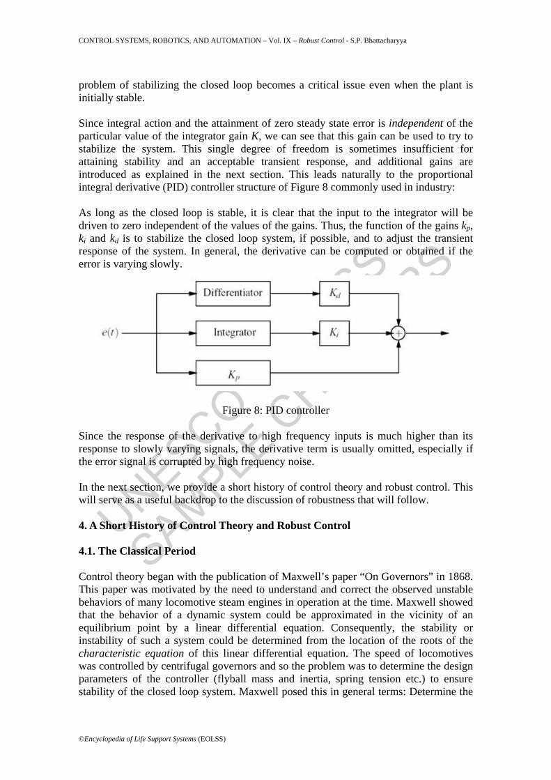
problem of stabilizing the closed loop becomes a critical issue even when the plant is initially stable. Since integral action and the attainment of zero steady state error is independent of the particular value of the integrator gain K, we can see that this gain can be used to try to stabilize the system. This single degree of freedom is sometimes insufficient for attaining stability and an acceptable transient response, and additional gains are introduced as explained in the next section. This leads naturally to the proportional integral derivative (PID) controller structure of Figure 8 commonly used in industry:

As long as the closed loop is stable, it is clear that the input to the integrator will be driven to zero independent of the values of the gains. Thus, the function of the gains kp, ki and kd is to stabilize the closed loop system, if possible, and to adjust the transient response of the system. In general, the derivative can be computed or obtained if the error is varying slowly.

Figure 8: PID controller Since the response of the derivative to high frequency inputs is much higher than its response to slowly varying signals, the derivative term is usually omitted, especially if the error signal is corrupted by high frequency noise. In the next section, we provide a short history of control theory and robust control. This will serve as a useful backdrop to the discussion of robustness that will follow. 4. A Short History of Control Theory and Robust Control 4.1. The Classical Period Control theory began with the publication of Maxwell’s paper “On Governors” in 1868. This paper was motivated by the need to understand and correct the observed unstable behaviors of many locomotive steam engines in operation at the time. Maxwell showed that the behavior of a dynamic system could be approximated in the vicinity of an equilibrium point by a linear differential equation. Consequently, the stability or instability of such a system could be determined from the location of the roots of the characteristic equation of this linear differential equation. The speed of locomotives was controlled by centrifugal governors and so the problem was to determine the design parameters of the controller (flyball mass and inertia, spring tension etc.) to ensure stability of the closed loop system. Maxwell posed this in general terms: Determine the

UNESCO – EOLS

S

SAMPLE C

HAPTERS



constraints on the coefficients of a polynomial that ensure that the roots are confined to the left half plane, the stability region for continuous time systems. This problem had actually been already solved for the first time by the French mathematician Hermite in 1856! In his proof, Hermite related the location of the zeros of a polynomial with respect to the real line to the signature of a particular quadratic form. In 1877, the English physicist E.J. Routh, using the theory of Cauchy indices and of Sturm sequences, gave his now famous algorithm to compute the number k of roots which lie in the right half of the complex plane Re(s) ≥ 0. This algorithm thus gave a necessary and sufficient condition for stability in the particular case when k = 0. In 1895, A. Hurwitz drawing his inspiration from Hermite’s work, gave another criterion for the stability of a polynomial. This new set of necessary and sufficient conditions took the form of n determinantal inequalities, where n is the degree of the polynomial to be tested. Equivalent results were discovered at the beginning of the century by I. Schur and A. Cohn for the discrete-time case, where the stability region is the interior of the unit disc in the complex plane. One of the main concerns of control engineers had always been the analysis and design of systems that are subjected to various types of uncertainties or perturbations. These may take the form of noise or of some particular external disturbance signals. Perturbations may also arise within the system, in its physical parameters. This latter type of perturbations, termed parametric perturbations, may be the result of actual variations in the physical parameters of the system, due to aging or changes in the operating conditions. For example in aircraft design, the coefficients of the models that are used depend heavily on the flight altitude. It may also be the consequence of uncertainties or errors in the model itself; for example, the mass of an aircraft varies between an upper limit and a lower limit depending on the passenger and baggage loading. From a design standpoint, this type of parameter variation problem is also encountered when the controller structure is fixed, but its parameters are adjustable. The choice of controller structure is usually dictated by physical, engineering, hardware and other constraints such as simplicity and economics. In this situation, the designer is left with a restricted number of controller or design parameters that have to be adjusted so as to obtain a satisfactory behavior for the closed-loop system; for example, PID controllers have only three parameters that can be adjusted. The characteristic polynomial of a closed-loop control system containing a plant with uncertain parameters will depend on those parameters. In this context, it is necessary to analyze the stability of a family of characteristic polynomials. It turns out that the Routh-Hurwitz conditions, which are so easy to check for a single polynomial, are almost useless for families of polynomials because they lead to conditions that are highly nonlinear in the unknown parameters. Thus, in spite of the fundamental need for dealing with systems affected by parametric perturbations, engineers were faced from the outset with a major stumbling block in the form of the nonlinear character of the Routh-Hurwitz conditions, which moreover was the only tool available to deal with this problem. One of the most important and earliest contributions to stability analysis under parameter perturbations was made by Nyquist in his classic paper of 1932 on feedback

UNESCO – EOLS

S

SAMPLE C

HAPTERS



amplifier stability. This problem arose directly from his work on the problems of long-distance telephony. This was soon followed by the work of Bode which eventually led to the introduction of the notions of gain and phase margins for feedback systems. Nyquist’s criterion and the concepts of gain and phase margin form the basis for much of the classical control system design methodology and are widely used by practicing control engineers. - - -

TO ACCESS ALL THE 28 PAGES OF THIS CHAPTER,

Click here

Bibliography Ackermann J. (1993). Robust Control: Systems with Uncertain Physical Parameters. New York, NY : Springer Verlag.

Barmish B. R. (1983). Stabilization of Uncertain Systems via Linear Control. IEEE Transactions on Automatic Control 28, 848-850.

Barmish B. R. (1994). New Tools for Robustness of Linear Systems. New York, NY : Macmillan Publishing Co.

Barmish B. R., Hollot C. V, Kraus F. J., and Tempo R. (1992). Extreme point results for robust stabilization of interval plants with first order compensators. IEEE Transactions on Automatic Control 37 (6), 707-714

Bartlett A. C., Hollot C. V., and Lin H. (1988). Root location of an entire polytope of polynomials: it suffices to check the edges. Mathematics of Controls, Signals and Systems 1, 61-71. [Proves the Edge Theorem.]

Bartlett A. C., Tesi A., and Vicino A. (1993). Frequency response of uncertain systems with interval plants. IEEE Transactions on Automatic Control 38 (6), 929-933. [Shows that the Kharitonov segments determine the frequency response envelopes.]

Bhattacharyya S. P. (1974). Disturbance Rejection in Linear Systems. International Journal of System Science 5, (7), 633-637.

Bhattacharyya S. P. (1987). Robust stabilization against structured perturbations, 172pp. New York : Springer-Verlag.

Bhattacharyya S. P. and deSouza E. (1982). Pole Assignment via Sylvester’s Equation. Systems & Control Letters 1 (4), 261-263. [Showed that pole assignment state feedback could be computed without transformation to canonical forms which are inherently unstable numerically.]

Bhattacharyya S. P. and Pearson J. B. (1972). On Error Systems and the Servomechanism Problem. International Journal of Control 15 (6), 1041-1062. Gave the first geometric solution of the servomechanism problem.

Bhattacharyya S. P., Chapellat H., and Keel L. H. (1995), 648pp. Robust Control: The Parametric Approach, 648. Upper Saddle River, New Jersey: Prentice Hall. [A comprehensive account of the parametric approach to Robust Control.]

Bhattacharyya S. P., del Nero Gomes A. C. and Howze J. W. (1983). The Structure of Robust Disturbance Rejection Control. IEEE Transactions on Automatic Control 28 (5), 874-881.

http://www.eolss.net/Eolss-sampleAllChapter.aspx

http://www.eolss.net/ebooklib/sc_cart.aspx?File=E6-43-14-00

UNESCO – EOLS

S

SAMPLE C

HAPTERS



Bhattacharyya S. P., Pearson, J. B., and Wonham W. M. (1972). On zeroing the output of a linear system. Information and Control 2, 135-142. [Lays the foundation for a geometric solution of the multivariable servomechanism problem.]

Bhattacharyya, S. P. and J. B. Pearson (1970). On the linear servomechanism problem. International Journal of Control 12 (5), 795-806.

Bhattacharyya, S. P. and Keel L. H. (ed.). (1991). Control of Uncertain Dynamic Systems. Littleton, MA : CRC Press. [Collection of papers on robust control presented at the 1991 International Workshop in San Antonio, Texas.]

Bode, H. W. (1945). Network Analysis and Feedback Amplifier Design. New York, NY : D. Van Nostrand Co.

Boyd S. P. and Barratt C. H. (1991). Linear Controller Design: Limits of Performance, 416 pp. Englewood Cliffs, NJ : Prentice Hall Publishing Co.

Brasch F. M. and Pearson J. B. (1970). Pole placement using dynamic compensator. IEEE Transactions on Automatic Control 15 (1), 34-43. [Established a fundamental upper bound on the order of stabilizing compensators.]

Burl J. B. (1998). Linear Optimal Control. Menlo Park, CA : Addison Wesley.

Chang B. C. and Pearson J. B. (1984). Optimal disturbance reduction in linear multivariable systems. IEEE Transactions on Automatic Control 29, 880-887. [Controller design based on minimizing the norm of the disturbance transfer function.]

Chapellat H. and Bhattacharyya S. P. (1989). A generalization of Kharitonov’s theorem: robust stability of interval plants. IEEE Transactions on Automatic Control 34 (3), 306-311. [Generalized Kharitonov’s Theorem to handle interval plants with fixed controllers.]

Chapellat H., Dahleh M., and Bhattacharyya S. P. (1990). Robust Stability under Structured and Unstructured Perturbations. IEEE Transactions on Automatic Control 35 (10), 1100-1108.

Chapellat H., Dahleh M., and Bhattacharyya S. P. (1991). On Robust Nonlinear Stability of Interval Control Systems. IEEE Transactions on Automatic Control. 36 (1), 59-67.

Chen M. J. and C. A. Desoer. (1984). Necessary and Sufficient Conditions for Robust Stability of Linear Distributed Feedback Systems. IEEE Transactions on Automatic Control 29, 880- 888.

Cohn A. (1922). Uber die Anzahl der Wurzein einer Algebraischen Gleichung in einem Kreise. Math. Zeit. 14, 110-148.

Dahleh M. A. and Pearson J. B. (1987). L1 optimal feedback controllers for MIMO discrete-time systems. IEEE Transactions on Automatic Control 32 (4), 314-322. [Solved the …1optimal control problem for discrete time systems.]

Dahleh M., Tesi A. and Vicino A. (1993). On the robust Popov criterion for interval Lur’e system, IEEE Transactions on Automatic Control 38 (9) 1400-1405.

Dahleh M., Tesi A., and Vicino A. (1992). Robust stability and performance of interval plants. Systems & Control Letters,Vol. 19, 353-363.

Datta A., Ho M.-T., and Bhattacharyya S.P. (2000). Structure and Synthesis of PID Controllers. London : Springer. [Determines the set of all PID controllers that stabilize a given linear time ivariant plant.]

Davison E. J. (1976). The robust control of a servomechanism problem for linear time-invariant systems. IEEE Transactions on Automatic Control 21 (1), 25-34.

deGaston R. R. E. and Safonov M. G. (1988). Exact Calculation of the Multiloop Stability Margin. IEEE Transactions on Automatic Control 33 (2), 156-171.

Dorato P. (1987). Robust Control. New York: IEEE Press. [A collection of important papers on Robust Control up to 1986.]

Dorato P. and Yedavalli R. K. (ed.). (1989). Recent Advances in Robust Control. New York : IEEE Press. [Collection of Robust Control papers concentrated mainly on the parametric approach.]

UNESCO – EOLS

S

SAMPLE C

HAPTERS



Dorato P., Fortuna L., and Muscato G. (1992) Robust Control for Unstructured Perturbations: An Introduction, Vol. 14. Springer Verlag. [Lecture Notes in Control and Information Sciences.]

Doyle J. C. (1982). Analysis of feedback systems with structured uncertainties. (Proceedings of IEE D), Vol. 129, (6), pp. 242-250.

Doyle J. C. and Stein G. (1979). Robustness with observers. IEEE Transactions on Automatic Control 24, 607-611.

Doyle J. C. and Stein G. (1981). Multivariable feedback design: Concepts for a classical/modern synthesis. IEEE Transactions on Automatic Control 26, 4-17.

Doyle J. C., Glover K., Khargonekar P. P., and Francis B. A. (1989). State Space Solution to Standard H2

and H∞ Control Problems. IEEE Transactions on Automatic Control 34 (8), 831-847. [Gave a solution of H2 and H∞ problems in terms of Ricatti equations.]

Doyle, J. C. (1978). Guaranteed margins for LQG regulators. IEEE Transactions on Automatic Control 23, 756-757.

Fan M. K. H., Tits A. L. and Doyle J. C. (1991). Robustness in the presence of mixed parametric uncertainty and unmodeled dynamics. IEEE Transactions on Automatic Control 36 (1), 25-38.

Ferreira P. M. G. (1976). The servomechanism problem and the method of the state space in the frequency domain. International Journal of Control 23 (2), 245-255.

Ferreira P. M. G. and Bhattacharyya S. P. (1977). On blocking zeros. IEEE Transactions on Automatic Control 22 (2), 258-259.

Francis B. A. and Wonham W. M. (1975). The internal model principle for linear multivariable regulators. Applied Mathematics and Optimization 2 (2), 170-194. [Established the necessity of error feedback and internal models for robust servomechanisms.]

Francis B. A. and Zames G. (1984). On H∞ optimal sensitivity theory for SISO feedback systems. IEEE Transactions on Automatic Control 29, 9-16.

Francis B. A., Helton J. W., and Zames, G. (1984). H8-optimal feedback controllers for linear multivariable systems. IEEE transactions on Automatic Control 29(10), 888-900.

Fu M. (1990). Computing the frequency response of linear systems with parametric perturbation, Systems & Control Letters 15, 45-52.

Glover K. (1986). Robust stabilization of linear multivariable systems: relations to approximation. International Journal Control 43, 741-766.

Hermite C. (1856). Sur le nombre de racines d’une équation algebrique comprise entre des limites données, J. Reine Angew. Math. 52, 39-51.

Hinrichsen D. and Martenson B. (ed.). 1990. Control of Uncertain Systems. Berlin : Birkhäuser.

Hinrichsen D. and Pritchard A. J. (1989). An application of state space methods to obtain explicit formulae for robustness measures of polynomials. Robustness in Identification and Control, (ed. M. Milanese, R. Tempo, A. J. A. Vicino A. J.) pp. 183-206. New York : Plenum.

Hinrichsen D. and Pritchard A. J. (1990). Real and complex stability radii: a survey. Control of Uncertain Systems, (ed. D. Hinrichsen and B. Maartensson), pp. 119 -162. Birkhauser.

Hollot C. V. and Tempo R. (1994). On the Nyquist envelope of an interval plant family. IEEE Transactions on Automatic Control 39 (2), 391-396.

Horowitz I. (1963). Synthesis of Feedback Control Systems. New York, NY : Academic Press.

Horowitz I. A. (1991). Survey of Quantitative Feedback Control. International Journal of Control 53, 255- 291.

Hurwitz A. (1895). Uber die Bedingungen, unter welchen eine Gleichung nur Wurzeln mit negativen reellen Teilen besitzt. Math. Ann. 46, 273-284.

Jayasuriya S., Yaniv O., Nwokah O. D. I., and Chait Y. (1992). Benchmark problem solution by

UNESCO – EOLS

S

SAMPLE C

HAPTERS



Quantitative Feedback Theory. Journal of Guidance, Control, and Dynamics 15 (5), 1087-1093.

Kalman R. E. (1960). Contribution to the Theory of Optimal Control. Boletim. de Sociedad Mexicana de Matematica Mexico, Ser 2, Vol. 5102-119.

Kalman R. E. (1964). When is a Linear Control System Optimal? ASME Transactions Series D, Vol 86, 51- 60.

Kalman R. E. and Bucy R. S. (1961). New Results in Linear Filtering and Prediction Theory, ASME Transactions 83, 95 -107.

Katbab, A. and Jury E. I. (1990). Robust Schur-stability of control systems with interval plants. International Journal of Control 51, (6), 1343-1352.

Keel L. H. and Bhattacharyya S. P. (1994). Robust parametric classical control design. IEEE Transactions on Automatic Control 39 (7), 1524-1530.

Keel L. H., Bhattacharyya S. P., and J. W. Howze. (1988). Robust control with structured perturbations. IEEE Transactions on Automatic Control 33 (1), 68 78.

Keel L.H. and Bhattacharyya S.P. (1997). Robust, Fragile or Optimal? IEEE Transactions on Automatic Control Vol. 42 (8), 1098-1105. [Showed by examples that optimal systems designed by H2 , H∞ , l1 and µ approaches can have extreme sensitivity to controller parameters.]

Keel L.H. and Bhattacharyya S.P. (1999). Robust stability and performance with fixed order controllers. Automatica 35 (10), 1717-1724.

Kharitonov V. L. (1978). Asymptotic stability of an equilibrium position of a family of systems of linear differential equations. Differential Uravnen 14, 2086-2088. [Translation in Differential Equations 14, 1483-1485. [Proved that four polynomials determine the Hurwitz stability of an interval polynomial family. This was translated in 1979.]

Kharitonov V. L. (1978). On a generalization of a stability criterion. Izvetiy Akademii Nauk Kazakhskoi SSR, Seria fizikomatematicheskaia 1, 53 57.

Kharitonov V. L. (1979). The Routh-Hurwitz problem for families of polynomials and quasipolynomials. Izvetiy Akademii Nauk Kazakhskoi SSR, Seria fizikomatematicheskaia 26, 69-79.

Kimura H. (1975). Pole Assignment by Gain Output Feedback. IEEE Transactions on Automatic Control. 20 (4), 509 516.

Kimura H. (1984). Robust Stabilizability for a Class of Transfer Functions. IEEE Transactions on Automatic Control 29 (9), 788 793.

Kraus, F. J., Anderson B. D. O. and Mansour M. (1988). Robust Schur polynomial stability and Kharitonov’s theorem. International Journal of Control 47, 1213-1225.

Kucera V. (1979). Discrete Linear Control: The Polynomial Equation Approach. New York : Wiley.

Kwakernaak H. (1991). The polynomial approach to H8optimal regulation. H8-Control Theory, Lecture Notes in Mathematics (ed. E. Möscaand and L. Pandolfi.), pp.141-221, Berlin : Springer Verlag.

Kwakernaak H. and Sivan R. (1972). Linear Optimal Control Systems. New York : Wiley-Interscience.

Lehtomaki N. A., Sandell N. R., and Athans M. (1981, 1982). Robustness Results in Linear Quadratic Gaussian Based Multivariable Control Designs. IEEE Transactions on Automatic Control 26, 75-92.

Leondes C. T.(ed.). (1992). Robust Control System Techniques and Applications. Control and Dynamics Systems, Vol. 50. New York, NY : Academic Press. [These two references contain a collection of papers on robustness.]

Leondes C. T.(ed.). (1992). Robust Control System Techniques and Applications. Control and Dynamics Systems, Vol. 51. New York, NY : Academic Press. [These two references contain a collection of papers on robustness.]

Luenberger D. G. (1971). An Introduction to Observers. IEEE Transactions on Automatic Control 16.

Lure A. I. (1957). On some nonlinear problems in the theory of automatic control. London : H. M.

UNESCO – EOLS

S

SAMPLE C

HAPTERS



Stationary Office. [Russian Edition, 1951.]

Maciejowski J. M.Multivariable Feedback Design. (1988). Reading, MA : Addison Wesley

Maxwell J. C. (1868). On Governors. Proceedings of the Royal Society. 16, 270-283. London, England.

Nyquist H. (1932). Regeneration theory. Bell System Technical Journal. 11, 126-147.

Pearson J. B. (1968). Compensator design for Dynamic Optimization. International Journal of Control. 9, 473.

Rantzer A. (1992). Stability Conditions for Polytopes of Polynomials. IEEE Transactions on Automatic Control 37, 79-89.

Rosenbrock H. H. (1970). State Space and Multivariable Theory, 257 pp. New York, N.Y: John Wiley & Sons.

Rosenbrock H. H. (1972). The stability of multivariable systems. IEEE Transactions on Automatic Control 17, 105-107.

Rosenbrock H. H. and McMorran V. (1971). Good, Bad, or Optimal. IEEE Transactions on Automatic Control. 16 (6), 552-554.

Routh E. J. (1877). A Treatise on the Stability of a Given State of Motion. London: Macmillan Publishing Co.

Safonov M. G. (1980). Stability and Robustness of Multivariable Feedback Systems. Cambridge, MA : MIT Press.

Safonov M. G. and Athans M. (1977). Gain and phase margins of multiloop LQG regulators. IEEE Transactions on Automatic Control 22, 173-179.

Schur I. (1918). Uber Potenzreichen, die in innern des Einheitkreises beschrankt sind. J. Reine Angew. Math. 147, 205-232.

Schur I. (1918).Uber Potenzreichen, die in innern des Einheitkreises beschrankt sind. J. Reine Angew. Math. 148, 122-145.

Boyd, S.P., El-Ghaoui, L., Feron, E.,Balakrishnan, V.. (Eds.) SIAM Frontier Series. (1994). Linear Matrix Inequality in Systems and Control Theory. Philadelphia, PA : SIAM. [Gives a comprehensive account of the LMI approach to robust and optimal control.] Siljak D. D. (1969). Nonlinear Systems: Parametric Analysis and Design. New York : Wiley.

Siljak, D. D. (1989). Parameter space methods for robust control design: a guided tour. IEEE Transactions on Automatic Control 34( 7), 674-688.

Siljak, Dragoslav D. (1969). Nonlinear Systems: The Parameter Analysis and Design. NY, John Wiley and Sons, Inc. [A detailed and important account of the parameter plane mapping approach to analysis and design of linear and nonlinear control systems.]

Stein G. and Athans M. (1987). The LQG/LTR procedure for multivariable feedback control design. IEEE Transactions on Automatic Control. 32, 105-114.

Stoorvogel A. A. (1992). The H8 Control Problem: A State Space Approach. Upper Saddle River: New Jersey Prentice-Hall.

Tesi A. and Vicino A. (1990). Robustness Analysis for linear dynamical systems with linearly correlated parameter uncertainties. IEEE Transactions on Automatic Control 35 (2), 186-190.

Tesi A. and Vicino A. (1991). Kharitonov segments suffice for frequency response analysis of plant controller families. Control of Uncertain Dynamic Systems, (ed. S. P. Bhattacharyya and L. H. Keel), Littleton, MA: CRC Press.

Tesi A. and Vicino A. (1991). Robust absolute stability of Luré’s control systems in parameter space. Automatica 27, 147-151.

Tsypkin Y. Z. and Polyak B. T. (1991). Frequency Domain Criteria for p-Robust Stability of Continuous Linear Systems. IEEE Transactions on Automatic Control. 36 (12), 1464-1469,

UNESCO – EOLS

S

SAMPLE C

HAPTERS



Tsypkin Y. Z. and Polyak B. T. (1992). Robust absolute stability of continuous systems. Robustness of Dynamic Systems with Parameter Uncertainties, (ed. M. Mansour., S. Balemi and W. Truöl.), pp, 113-124. Berlin : Birkhäuser.

Vicino A., Tesi A., and Milanese M. (1990).Computation of nonconservative stability perturbation bounds for systems with nonlinearly correlated uncertainties. IEEE Transactions on Automatic Control 35 (7), 835 841.

Vidyasagar M. (1985). Control System Synthesis: A Factorization Approach. Cambridge, MA : MIT Press.

Vidyasagar M. (1986). Optimal rejection of persistent bounded disturbances. IEEE Transactions on Automatic Control 31 (6).

Vidyasagar M. and Kimura H. (1986). Robust controllers for uncertain linear multivariable systems. Automatica 22 (1).

Wonham,W. M. (1985). Linear Multivariable Control: a Geometric Approach, 3rd Edition, 334pp. New York : SpringerVerlag. [2nd Edition, 1985. Expositon of the geometric approach. Develops the Internal Model Principle, for robust servomechanisms.]

Youla D. C., Jabr H. A., and Bongiorno J. J. (1976). Modern Wiener-Hopf Design of Optimal Controllers—Part I: The Single Input Single Output Case. IEEE Transactions on Automatic Control 21, 3-13.

Youla D. C., Jabr H. A., and Bongiorno J. J. (1976). Modern Wiener-Hopf Design of Optimal Controllers—Part II: The Multivariable Case. IEEE Transactions on Automatic Control 21, 319-338. [These two papers introduced the Youla-Bongiorno-Jabr-Kucera(YJBK) parametrization.]

Zadeh L. A. and Desoer C. A. (1963). Linear Systems Theory. New York : McGraw Hill.

Zames G. (1981). Feedback and Optimal Sensitivity: Model Reference Transformations, Multiplicative Seminorms, and Approximate Inverses. IEEE Transactions on Automatic Control 26, 301-320.

Zames, G. (1963). Functional Analysis Applied to Nonlinear Feedback Systems. IEEE Transactions on Circuit Theory, vol. CT-10, 392-404. [Introduced the small gain theorem.]

Zames, G. and Francis B. A. (1983). Feedback, Minimax Sensitivity, and Optimal Robustness, IEEE Transactions on Automatic Control. 28, 585-601.

Zeheb E. (1990). Necessary and sufficient condition for the robust stability of a continuous systems: the continuous dependency case illustrated by multilinear dependence. IEEE Transactions on Circuits and Systems 37, 47- 53.

Zhou, K., Doyle J.C., and Glover, K. (1996). Robust and Optimal Control. Upper Saddle River, New Jersey: PrenticeHall. [A detailed account of H2 , H∞ and µ theory.] Biographical Sketch Shankar P. Bhattacharyya was born in Rangoon, Burma, on June 23, 1946. He obtained his undergraduate education (1962-1967) at the Indian Institute of Technology, Bombay, and graduate education, (M.S., Ph.D, 1967-1971) at Rice University, Houston. He established the graduate Program in Automatic Control at the Federal University, Rio de Janeiro, Brazil during 1971-1980 and was Chairman of the Department of Electrical Engineering from 1978 to 1980. In 1974-1975 he was a National Academy of Sciences Research Fellow at the NASA Marshall Space Flight Center. In 1980 he joined Texas A&M University, College Station, where he is presently Professor of Electrical. Engineering From 1990-1992 he served as Director of the Systems and Control Institute. In 1990, 1991 and 1992, respectively, he received the Texas Engineering Experiment Station Fellowship, the Halliburton Award of Excellence and the Dresser Industries Professorship from Texas A&M University. He served as an Associate Editor of the IEEE Transactions on Automatic Control in 1985-1986, and a member of the IEEE Control Systems Society Board of Governors. He was a Senior Fullbright Lecturer in 1989 and a UNDP consultant to the Government of India in 1990. In 1998 he received the Boeing Welliver Faculty Award. He held visiting lecturing assignments in Italy, Germany, France, India, Brazil, Mexico and Japan. In 1989 he was elected a Fellow of the IEEE for contributions to linear control system analysis and

UNESCO – EOLS

S

SAMPLE C

HAPTERS



design. He has made a number of original contributions to Control Theory and Engineering. These are documented in 4 books, 80 journals and over 100 conference papers in the field of Automatic Control, authored or co-authored by him. Dr. Bhattacharyya other interests include playing Indian classical music on the Sarode. He is a disciple, since 1982, of the renowned Sarode maestro Ustad Ali Akbar Khan and regularly performs as a concert artist in USA, India and Europe.

Robust Control - ENCYCLOPEDIA OF LIFE SUPPORT ... – EOLSS SAMPLE CHAPTERS CONTROL SYSTEMS,...

Documents

Transcript of Robust Control - ENCYCLOPEDIA OF LIFE SUPPORT ... – EOLSS SAMPLE CHAPTERS CONTROL SYSTEMS,...