Robust Boundary Layer Mesh Generation

Adrien Loseille1 and Rainald Lohner2

1 GAMMA Team, INRIA Paris-Rocquencourt, France Adrien.Loseille@inria.fr2 CFD Center, George Mason University, USA rlohner@gmu.edu

Summary. In this paper, we introduce a 3D local operator that automaticallycombines typical simpler operators as removal of vertices, collapse of edges or swapof faces and edges. This operator is inherited from incremental methods where themesh Hk is modified iteratively through sequences of insertion of a point P :

Hk+1 = Hk − CP + BP ,

where CP is the cavity of P and BP the ball of P . We derive two algorithms tocompute Cp. The first algorithm is tuned to be a fast point reprojection to thegeometry even in the presence of a boundary layer mesh. The second one is tunedto generate boundary layer meshes for complex geometries. We show how quasi-structured elements can be enforced. In addition, enhancements as multi-normalscan be incorporated in the process. Both operators can be used with surface andvolume point while preserving a given geometry. They rely on the use on an existinginitial volume mesh and always produce a valid 3D mesh on output.

Key words: Boundary layer mesh generation; mesh adaptation; incremental meth-ods; surface projection; CAD

1 Introduction

A boundary layer mesh is a quasi-structured layered mesh around a given geometry.It is usually considered as an extrusion of the initial surface along its normals [4,11, 12, 21] or by local modifications of the mesh [17]. These meshes are widelyused in Computational Fluid Dynamics (CFD) [23]. Indeed, most of commonly-used second-order unstructured CFD numerical schemes or commercial packagesneed a boundary layer mesh to accurately approximate the speed profile around abody during a viscous simulation, see the pioneering works [8, 11, 21]. The qualityof the mesh is also crucial as it has a huge impact on the evaluation of functionalsof interest used in industry as lift or drag. This is especially true for unstructuredflow solver [18], and thus for complex geometries for which defining a structured gridis no more tractable. Consequently, several severe difficulties need to be tackled togenerate a boundary layer mesh that is well suited for numerical computations.

2 Adrien Loseille and Rainald Lohner

State-of-the-art and problematics

The first difficulty is to deal with the required very high aspect ratios of the elementsO(103 − 105) along with a high-fidelity geometry: landing gear, full aircraft, . . . , seeFigure 1 for some examples. Using the normals as sole extrusion information requiresseveral enrichments to obtain a smooth layers transition on complex surfaces [1, 6,9, 10]. These techniques rely on a complex pre-processing of the surface in order toextract additional geometric information as convex or concave ridges. For instance,it may be required to handle normal deactivation in areas where the level of detailsis smaller than the size of the first layer or to add several normals to increase thequality of the boundary layer mesh, see Figure 2. In our approach, we use the optimalnormal computation of [2]. We replace the classical laplacian smoothing of normalsby defining a normal merging. In addition, the normals are not computed once forall layers, but are reevaluated after each layer insertion.

Fig. 1. Examples of complex geometries, a front landing gear (left) and the back ofa missile (right). These geometries have a level of details that makes more complexthe generation of a boundary layer mesh.

The second difficulty arises once the boundary layer extrusion process is finished. In-deed, in most methods, a global mesh generation process is used to close the volume.Both constrained Delaunay-based methods [7] or frontal methods [13] are susceptibleto fail in presence of anisotropic or bad-shaped faces. We remove this weakness bygenerating the boundary layer mesh with local mesh modification operators. Con-sequently, we can guarantee that the process cannot fail, so that a computation isalways possible even though the generated mesh may be sub-optimal.

Finally, in the aforementioned methods, the boundary layer mesh generation isthought as a unique pre-processing procedure that is done prior to any computations.In particular, these methods are not sought to work in an adaptive context where the(surface) mesh is modified iteratively during the adaptation. When an adaptationis performed, simpler strategies have been devised as keeping the boundary layermesh unchanged [20]. However, in many applications, adapting the (surface andvolume) mesh seems mandatory to get the full picture of the physics as anisotropic

Robust Boundary Layer Mesh Generation 3

Fig. 2. F117 geometry (left) and closer view around two complex corners where itis impossible to find a unique normal seen by all the faces surrounding the corner(right).

phenomena (shocks, contact discontinuity, . . . ) interact with the boundary layer, seeFigure 3. In addition, asymptotic mesh convergence (one of the criteria to assess anumerical computation) is rarely observed on complex geometries with unstructuredtailored meshes [22]. Consequently, achieving a full coupling between boundary layermesh generation and mesh adaptation is tedious and remains a challenge. We pro-pose a first improvement in this context by defining a fast point re-projection evenif the current mesh has a very thin boundary layer mesh. This operation is manda-tory to adapt the surface mesh especially in strategies that keep a valid volumemesh [14, 15, 19]. In addition, the local operator used to generate the boundarylayer may be used on anisotropic surface. By using local modification operators, wealso remove the need of calling a global mesh generator during the adaptive process.

Fig. 3. A supersonic viscous bullet (left) from NASA media library and adap-tive shock/boundary layer interaction (rigth) excerpt from [16]. Both examples con-tain interaction between the viscous boundary layer and anisotropic phenomena (redsquares).

4 Adrien Loseille and Rainald Lohner

Outline

We first end this introduction with the nomenclature and definitions used throughoutthe paper. In Section 2, we introduce a point re-inserter procedure that can be usedto project a point back to a given geometry or to generate a mono-normal boundarylayer mesh. In Section 3, we show how this operator is modified to allow to generatequasi-structured boundary layer meshes. The procedure to generate one layer (choiceof normals, multi-normals, . . . ) is also recalled. We validate this approach on severalcomplex geometries.

Nomenclature and definitions

In what follows, H is a 3D simplicial mesh, i.e., composed only of tetrahedra andtriangles. H is valid if all tetrahedra have a positive volume. If an hybrid meshis given as input, it is pre-processed to be decomposed into a simplicial mesh. Wefollow the procedure given in [5].

Capital letters as A, B, . . . , P denote points of R3, except K that usually denotesan element (triangle or tetrahedron). BP is the ball of P , i.e., the list of elementssurrounding P (having P as vertex), SAB is the shell of edge AB, i.e., the list ofelements having A and B as vertices. Topological entities as balls and shells arecomputed on the fly by using the elements surrounding elements storage data struc-ture. Consequently, we assume that for each tetrahedron, we know the neighboringtetrahedra (or boundary faces) seen across the 4-faces. We refer to [7] for moredetails.

Cp is the cavity of P . This notion is usually related to Delaunay mesh generation. Weuse this nomenclature to keep the analogy with incremental method and Delaunaypoint insertion. However, in this paper, the cavity is just a set of tetrahedra and isnot related to any Delaunay criteria. Instead, we assume that Cp has the followingproperty:

Given any two tetrahedra K1 andK2 in Cp,

there exists a path trough faces’ of tetrahedra in Cp

that links K1 and K2.

(1)

Note that this property holds for the balls of vertices and the shells of edges. Wedenote by CP the external faces of CP . It is composed of boundary faces (triangles)and internal faces. For each internal face CP , the neighboring tetrahedron viewedfrom this face is not contained in CP .

Given an oriented face [A,B,C] and a normal n, the visibility of n with respect to[A,B,C] is the dot product between n and the normal to the face. In a similar way,a point P is visible for an oriented face [A,B,C] if the volume of the tetrahedron[P,A,B,C] is positive.

We now state the fundamental property: Given a valid mesh H, a point P and aset CP , if (3) holds for CP and P is visible for all faces of CP then the mesh given byH− CP + BP is valid. The local mesh modification operators derived in this paperare based on this property.

Robust Boundary Layer Mesh Generation 5

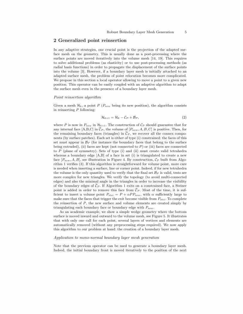
2 Generalized point reinsertion

In any adaptive strategies, one crucial point is the projection of the adapted sur-face mesh on the geometry. This is usually done as a post-processing where thesurface points are moved iteratively into the volume mesh [14, 19]. This requiresto solve additional problems (as elasticity) or to use post-processing methods (asradial basis functions) in order to propagate the displacement of the surface pointsinto the volume [3]. However, if a boundary layer mesh is initially attached to anadapted surface mesh, the problem of point relocation becomes more complicated.We propose in this section a local operator allowing to move a point to a given newposition. This operator can be easily coupled with an adaptive algorithm to adaptthe surface mesh even in the presence of a boundary layer mesh.

Point reinsertion algorithm

Given a mesh Hk, a point P (Pnew being its new position), the algorithm consistsin reinserting P following:

Hk+1 = Hk − CP + BP , (2)

where P is now in Pnew in Hk+1. The construction of CP should guarantee that forany internal face [A,B,C] in CP , the volume of [Pnew, A,B,C] is positive. Then, forthe remaining boundary faces (triangles) in CP , we recover all the connex compo-nents (by surface patches). Each set is either of type (i) constrained: the faces of thisset must appear in BP (for instance the boundary faces that belong to the surfacebeing extruded), (ii) faces are kept (not connected to P ) or (iii) faces are connectedto P (plane of symmetry). Sets of type (i) and (ii) must create valid tetrahedrawhereas a boundary edge [A,B] of a face in set (i) is triangulated to create a newface [Pnew, A,B], see illustration in Figure 4. By construction, CP built from Algo-rithm 1 verifies (3). If this algorithm is straightforward for volume point, more careis needed when inserting a surface, line or corner point. Indeed, if for new tetrahedrathe volume is the only quantity used to verify that the final set BP is valid, tests aremore complex for new triangles. We verify the topology (to avoid multi-connectededges) and also the minimal angle in the triangles in order to increase the visibilityof the boundary edges of CP . If Algorithm 1 exits on a constrained face, a Steinerpoint is added in order to remove this face from CP . Most of the time, it is suf-ficient to insert a volume point Pstei = P + αPPnew, with α sufficiently large tomake sure that the faces that trigger the exit become visible from Pstei. To completethe reinsertion of P , the new surface and volume elements are created simply bytriangulating each boundary face or boundary edge with Pnew.

As an academic example, we show a simple wedge geometry where the bottomsurface is moved inward and outward to the volume mesh, see Figure 5. It illustratesthat with only one call for each point, several layers of vertices and elements areautomatically removed (without any preprocessing steps required). We now applythis algorithm to our problem at hand: the creation of a boundary layer mesh.

Application to mono-normal boundary layer mesh generation

Note that the previous operator can be used to generate a boundary layer mesh.Indeed, the initial boundary front is moved iteratively to the position of the next

6 Adrien Loseille and Rainald Lohner

Algorithm 1 Cavity enlargement for P and new position Pnew

Initialize the cavity with the ball of P : CP = BP

Volume Part:For each K in CP

For each internal face [A,B,C] of K such that P /∈ [A,B,C]:if [A,B,C] is a boundary face then update CP

else if volume of [Pnew, A,B,C] ≤ 0, add neighboring tetrahedron to CP

endifEndFor

EndFor

Surface Part:Create the sets of connex components of the boundary face of CP

Set type (i), (ii) or (iii) for each componentCheck that all faces of type (i) or (ii) produce a valid tetrahedron, otherwise exitFor each component Cmp of type (iii)

For each triangle K in Cmp

For each edge [A,B] of K with P /∈ [A,B]if [A,B] is a boundary edge of Cmp then test triangle [Pnew, A,B]

if the triangle is not valid then add shell SAB to CP

endifendif

EndFor

EndForif CP is modified goto Volume Part.

layer. The boundary layer mesh is then stored separately from the remaining volumemesh. Each face of the initial front engenders either a prism (if all the points of theface are moved), or a pyramid (if only two points of the face are moved), or atetrahedron (if only one point of the face is moved). The final mesh is obtainedby gathering these two parts. If a simplicial mesh is required for computations,we decompose the hybrid entities into tetrahedra [5]. Note that the front is moved(extruded) along one (normal) direction. Consequently, several passes of laplaciansmoothing are done on these directions in order to improve the quality of the layersat opened ridges (along the trailing edge for instance). This strategy is equivalent tomoving mesh methods used to generate boundary layer meshes as in [3, 4]. However,in our approach, we do not need to solve a global PDE (elasticity, . . . ) to propagatethe boundary displacement into the volume. The necessary room to move the pointis created automatically by the local operator. We give two examples of boundarylayer mesh generation applied to an initial anisotropic m6 wing and to a shuttle,see Figures 6 and 7. Despite the high-level of anisotropy (on the surface and volumemesh), the reinserter succeeds to move the front. For each case, we emphasize typicalareas where multi-normals seems mandatory to improve the overall quality of theboundary layer mesh, see the red squares in Figures 6 and 7. The CPU time for

Robust Boundary Layer Mesh Generation 7

P

Pnew

type (iii)

type (ii)

type (i)

Fig. 4. An example of the boundary faces of CP for P with new position Pnew. Eachcolor defines a connex component. Depending on the type, either a tetrahedron isgenerated or a triangle, see white entities.

each case is less that 1 min on a macbook pro laptop equipped with an i7 core at2.66Ghz with 8 Gb of Ram.

The main drawback of this approach is to handle two separate meshes. Addingmulti-normals enhancement for instance is also tedious with this approach. Indeed,as soon as the surface front is modified, the matching with the two meshes is nottrivial anymore. Consequently, we prefer to define a new local operator that hasmuch more flexibility and that removes the need to store two meshes.

3 Boundary layer mesh generation

We consider in this Section the generation of a boundary layer mesh starting froma given surface mesh. We focus only on the generation of the volume mesh meaningthat the surface mesh that supports the boundary layer is kept constant duringthe whole process. No hypothesis is made on the features of the surface mesh. Inparticular, the process should handle anisotropic surface meshes.We first modify the previous reinserter to become an inserter. We then exemplifyspecific choices of CP leading to the generation of quasi-structured elements. Themain improvement from the method described in Section 2 is to avoid to handletwo distinct meshes while offering more flexibility in the generation of the boundarylayer.

Boundary layer mesh generation by point insertion

Previous inserter is now turned into a constrained point inserter. We detail the mainmodifications.When Pnew is inserted along a normal, the previously created elements that are inthe boundary layer mesh should be kept. Consequently, a set K of (constrained)

8 Adrien Loseille and Rainald Lohner

Fig. 5. Example of a wedge geometry where the bottom surface (in blue) is movedalong the normals according to a sine (top) and parabola functions (bottom). In oneshot, large areas of the volume mesh are automatically removed.

tetrahedra in the boundary layer is created and updated after each insertion. Thecavity enlargement procedure of Algorithm 1 can exit if during the process a con-strained element is added to CP . The cavity initialization is also modified to removefrom BP elements that belong to K. In order to ensure (3), it is necessary to verifythat BP minus the constrained elements is still connex. From a technical point ofview, as Pnew is not initially (topologically) present in the mesh (contrary to thecase where P is moved), the main difficulty is related to the surface part of Algo-rithm 1. Indeed, every boundary face [A,B,C] will never contain Pnew, so additionalinformation is required to derive each connex component type. We can now statethe main result:

In a mono-normal context, previous inserter with initialization Cp = BP −K,

automatically generates quasi-structured elements.(3)

We first remark that if Pnew is inserted along a normal direction issued from P ,the final mesh will contain the edge PPnew. Then if face [A,B,C] belongs to CP ,then tetrahedron [A,B,C, Pnew] is created. Consequently, given a face [A,B,C] withthe extruded vertices [Anew, Bnew, Cnew], insertion of Anew will create tetrahedron

Robust Boundary Layer Mesh Generation 9

Fig. 6. Example of a boundary layer from an anisotropic m6-wing geometry. Evenin the presence of high anisotropy, the local operator succeeds to move the front point.The quality of the layers is decreasing at open ridges despite the use of a normalsmoothing (top right).

K1 = [A,B,C,Anew], insertion of Bnew will create K2 = [Anew, Bnew, B, C] andinsertion of Cnew will create K3 = [Cnew, Anew, Bnew, C]. The union of K1,K2 andK3 forms the prism [A,B,C,Anew, Bnew, Cnew]. Note that K1,K2 and K3 shouldbe added to K after each insertion. The update of K is based on the different setsof hybrid elements than can be created, see Figure 8. We illustrate in Figure 9,different prisms construction around the ball of a point. Note that changing theorder of insertion of the extruded points will lead to different decompositions ofthe prismatic mesh. Consequently, the point insertion can be a priori optimized inorder to favor the creation of the smallest diagonal edges when a quadrilateral faceof a prism is decomposed. In addition, according to the current configuration, theremaining points cannot be inserted in any order as this may lead to an invaliddecomposition (known as the Schonhardt’s prism). It is thus necessary to loop overthe remaining points in order to solve this issue. Usually, no more than 10 iterationsare required to insert all the points.

Possible enhancements with multi-normals and merge

Two main drawbacks of using only one normal per point arise at closed and openedridges. At closed ridges, the normals may cross, leading to invalid elements. At

10 Adrien Loseille and Rainald Lohner

Fig. 7. Example of a boundary layer from a shuttle geometry based on the displace-ment of a front layer along one normal. The quality of the layers is decreasing atopened ridges despite the use of a normal smoothing (bottom).

opened ridges, the quality of the elements decreases as the deviation between thenormals may be large. A common practice to solve this issue is to smooth thenormals [1]. In our approach, we can choose different initialization of CP in order toimprove the boundary layer mesh quality.In order to reduce the number of invalid elements, we pre-process the given normalsand current size and predict the volume of elements. For each invalid element found,we attempt to collapse the normals until no more negative element is found. For aface, if three normals are merged, a tetrahedron is created, whereas a pyramid iscreated when two normals are merged. Normals are merged according to a minimaldistance criterion. If we denote by (Pi)i=1,k the list of points associated with a givenlist of merged normals, the cavity is then initialized by

�BPi − K. The standard

Robust Boundary Layer Mesh Generation 11

Fig. 8. Depending on the configuration of normals, different kinds of prisms arerecovered: vertex-based (left), edge-based (middle) and face-based (right).

Fig. 9. Tow examples of the automatic process of prisms creation around a point.The final decomposition of prisms (in tetrahedra) depends on the order of the inser-tion of points.

inserter is then called with this initialization. We illustrate this operator on a simplecube geometry where 2 faces support the boundary layer mesh. Theses surfacesare adapted to follow the normal size distribution. Consequently, without normalsmoothing, normals cross each other at each step. We can see that the quality ofthe generated boundary layer mesh is improved with the merge of normals, seeFigure 10.The multi-normal case is the most complicated. The way the cavity CP is initializedis crucial to ensure the desired connectivity. Given P and a (minimal) set of normals,we start from the list of the (interface) faces that surround P . Interface faces are theboundary triangles for the first layer and then become the internal faces definingthe frontier between the previous and current layers. Note that this faces are partof CP . We then assign each face to a normal by trying to maximize the visibility.In addition, for a given normal, the list of faces should be adjacent by edges. If twomany normals are given, remaining normals with no more faces are not inserted.For a normal n associated to the list of face L = (Fi)i, the cavity is initialized byCP =

�AB∈Fi,Fj

SAB , where AB is an edge shared by two faces of L. The inserter

is then called normally with this initial choice of CP . We illustrate this procedureon a simple opened ridge. Fully structured elements are automatically created as inthe merged case, see Figure 11.The main difficulty when using merged and multi-normals consists in the recoveryof constrained elements in order to update K. In the mono-normal context, onlyface prisms are recovered whereas in this case, constrained elements can be also

12 Adrien Loseille and Rainald Lohner

point-based and edge-based, see Figure 8. Algorithm 2 summarizes the completeprocess.

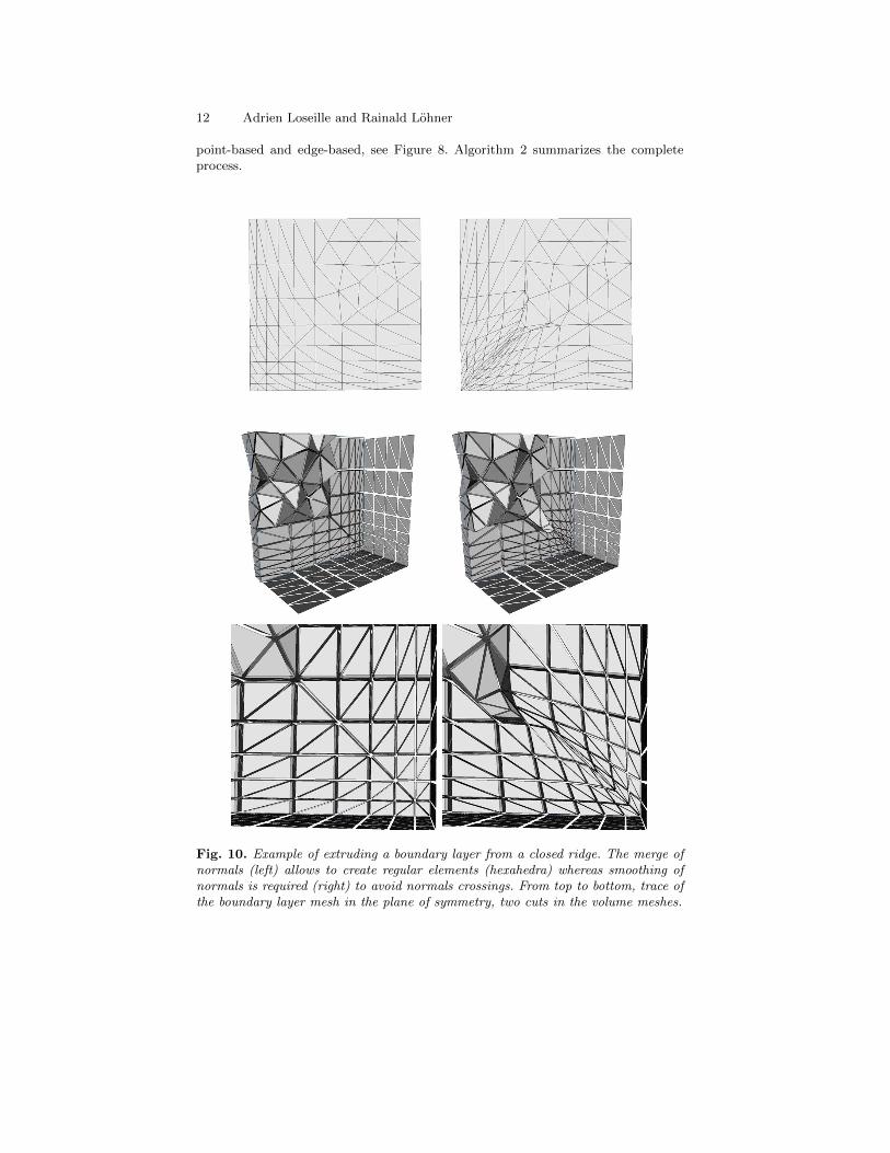
Fig. 10. Example of extruding a boundary layer from a closed ridge. The merge ofnormals (left) allows to create regular elements (hexahedra) whereas smoothing ofnormals is required (right) to avoid normals crossings. From top to bottom, trace ofthe boundary layer mesh in the plane of symmetry, two cuts in the volume meshes.

Robust Boundary Layer Mesh Generation 13

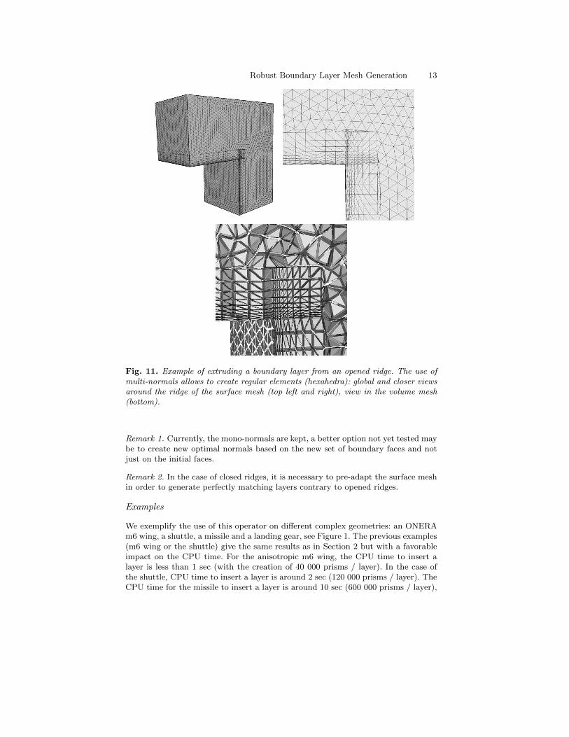
Fig. 11. Example of extruding a boundary layer from an opened ridge. The use ofmulti-normals allows to create regular elements (hexahedra): global and closer viewsaround the ridge of the surface mesh (top left and right), view in the volume mesh(bottom).

Remark 1. Currently, the mono-normals are kept, a better option not yet tested maybe to create new optimal normals based on the new set of boundary faces and notjust on the initial faces.

Remark 2. In the case of closed ridges, it is necessary to pre-adapt the surface meshin order to generate perfectly matching layers contrary to opened ridges.

Examples

We exemplify the use of this operator on different complex geometries: an ONERAm6 wing, a shuttle, a missile and a landing gear, see Figure 1. The previous examples(m6 wing or the shuttle) give the same results as in Section 2 but with a favorableimpact on the CPU time. For the anisotropic m6 wing, the CPU time to insert alayer is less than 1 sec (with the creation of 40 000 prisms / layer). In the case ofthe shuttle, CPU time to insert a layer is around 2 sec (120 000 prisms / layer). TheCPU time for the missile to insert a layer is around 10 sec (600 000 prisms / layer),

14 Adrien Loseille and Rainald Lohner

Algorithm 2 Boundary layer mesh generationWhile ( 1 )

1. Recover the interface surface mesh (between current layer and previous layer)2. Compute normals and multi-normals3. Fictive extrusion of the boundary-layer : optimize the layer with the merge of

normals4. Insert extruded points in the following order:

• along merged normals• along multi-normals• along mono-normals to close the boundary layer volume

5. Optimize the current layer: diagonal swapping and point smoothing

EndWhile

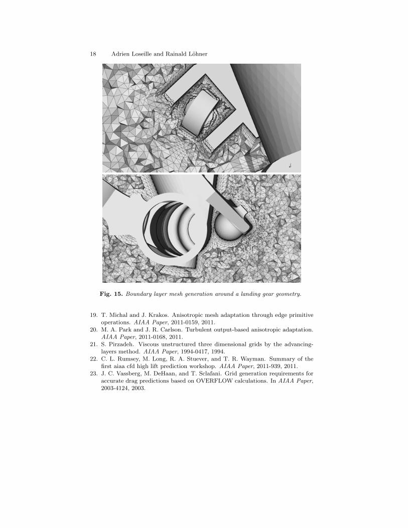
see Figures 12 and 13. For the landing gear geometry, the CPU time to insert a layerspans from 8 sec to 35 sec when all the points are inserted (e.g. 800 000 prisms /layer), see Figures 14 and 15. For 25 layers, the total CPU time is around 7 min.Note that the remaining volume mesh between the boundary layer mesh and theouter surface of the domain is not optimized neither in quality nor in size. This isdone in a different optimization step allowing to adapt the mesh with respect to agiven anisotropic metric field or to a uniformly graded metric. Consequently, we cansee that the process can insert a boundary layer mesh in an already high densitymesh, see Figure 14, but also in a very coarse mesh, see Figure 12.

4 Conclusion

A local point reinsertion operator is introduced. It can be used to project surfacepoints back to the geometry and to generate mono-normal boundary layer mesh. It isbased on simple topological principles with iterative checks on the validity of the finalsurface and volume mesh. This operator is then slightly modified in order to favorthe creation of quasi-structured elements. More insight into the initialization of Cp

allows to insert multi-normals and merged normals. This has a favorable impact onthe overall quality of the boundary layer grids. The generation of the boundary layermesh does not require the use of a global mesh generator to close the volume mesh.In addition, there is not check of face-face intersections as usually used when theboundary layer is extruded in an empty space. These features increase the robustnessof the method. Finally, the operator keeps its properties and robustness even in thepresence of highly stretched elements in the initial mesh. This point is a necessaryproperty to consider adaptive viscous simulations.

The current work is directed at improving the robustness for the multi-normals andmerged of normals. We also seek specific surface mesh adaptation. We also workon improving the transition from the boundary layer mesh to the volume mesh.The final intent is to derive an anisotropic mesh adaptation procedure to accuratelycapture viscous and anisotropic phenomena.

Robust Boundary Layer Mesh Generation 15

Fig. 12. Boundary layer mesh generation around a complex missile geometry start-ing from a coarse initial volume mesh.

References

1. R. Aubry and R. Lohner. Generation of viscous grids with ridges and corners.AIAA Paper, 2007-3832, 2007.

2. R. Aubry and R. Lohner. On the most normal normal. Communications inNumerical Methods in Engineering, 24(12):1641–1652, 2008.

3. T. Baker and P Cavallo. Dynamic adaptation for deforming tetrahedral meshes.AIAA Journal, 19:2699–3253, 1999.

4. C.L. Bottasso and D. Detomi. A procedure for tetrahedral boundary layer meshgeneration. Engineering Computations, 18:66–79, 2002.

16 Adrien Loseille and Rainald Lohner

Fig. 13. Boundary layer mesh generation around a complex missile geometry.

5. J. Dompierre, P. Labbe, M.-G. Vallet, and R. Camarero. How to subdivide pyra-mids, prisms, and hexahedra into tetrahedra. In Proc. of 8th Meshing Rountable,pages 195–204, 1999.

6. R.V. Garimella and M.S. Shephard. Boundary layer mesh generation for viscousflow simulations. Int. J. Numer. Meth. Fluids, 49:193–218, 2000.

7. P.-L. George and H. Borouchaki. Delaunay triangulation and meshing : appli-cation to finite elements. Hermes Science, Paris, Oxford, 1998.

8. O. Hassan, K. Morgan, E. J. Probert, and J. Peraire. Unstructured tetrahe-dral mesh generation for three-dimensional viscous flows. Int. J. Numer. Meth.Engrg., 39(4):549–567, 1996.

9. Y. Ito and K. Nakahashi. Unstructured mesh generation for viscous flow com-putations. In Proc. of 11th Meshing Rountable. Springer, 2002.

10. Y. Ito and K. Nakahashi. An approach to generate high quality unstructuredhybrid meshes. AIAA Paper, 2006-0530, 2006.

11. R. Lohner. Matching semi-structured and unstructured grids for Navier-Stokescalculations. AIAA Paper, 1993-3348, 1993.

Robust Boundary Layer Mesh Generation 17

Fig. 14. Boundary layer mesh generation around a landing gear geometry.

12. R. Lohner. Generation of unstructured grids suitable for RANS calculations.AIAA Paper, 1999-0662, 1999.

13. R. Lohner and P. Parikh. Three-dimensionnal grid generation by the advancing-front method. Int. J. Numer. Meth. Fluids, 8(8):1135–1149, 1988.

14. A. Loseille and R. Lohner. On 3d anisotropic local remeshing for surface, vol-ume, and boundary layers. In Proc. of 18th Meshing Rountable, pages 611–630.Springer, 2009.

15. A. Loseille and R. Lohner. Adaptive anisotropic simulations in aerodynamics.AIAA Paper, 2010-169, 2010.

16. A. Loseille and R. Lohner. Boundary layer mesh generation and adaptivity.AIAA Paper, 2011-0894, 2011.

17. D. L. Marcum. Adaptive unstructured grid generation for viscous flow applica-tions. AIAA Journal, 34(8):2440–2443, 1996.

18. D.J. Mavriplis. Results from the 3rd Drag Prediction Workshop using NSU3Dunstructured mesh solver. In AIAA Paper, volume 2007-0256, 2007.

18 Adrien Loseille and Rainald Lohner

Fig. 15. Boundary layer mesh generation around a landing gear geometry.

19. T. Michal and J. Krakos. Anisotropic mesh adaptation through edge primitiveoperations. AIAA Paper, 2011-0159, 2011.

20. M. A. Park and J. R. Carlson. Turbulent output-based anisotropic adaptation.AIAA Paper, 2011-0168, 2011.

21. S. Pirzadeh. Viscous unstructured three dimensional grids by the advancing-layers method. AIAA Paper, 1994-0417, 1994.

22. C. L. Rumsey, M. Long, R. A. Stuever, and T. R. Wayman. Summary of thefirst aiaa cfd high lift prediction workshop. AIAA Paper, 2011-939, 2011.

23. J. C. Vassberg, M. DeHaan, and T. Sclafani. Grid generation requirements foraccurate drag predictions based on OVERFLOW calculations. In AIAA Paper,2003-4124, 2003.