
ROBUST AND ACCURATE DIAPHRAGM BORDER DETECTION IN … · ROBUST AND ACCURATE DIAPHRAGM BORDER...
35
Master in Artificial Intelligence (UPC-URV-UB) Master of Science Thesis ROBUST AND ACCURATE DIAPHRAGM BORDER DETECTION IN CARDIAC X-RAY ANGIOGRAPHIES Simeon Petkov Advisors: Carlo Gatta and Petia Radeva Juny 2012
Transcript of ROBUST AND ACCURATE DIAPHRAGM BORDER DETECTION IN … · ROBUST AND ACCURATE DIAPHRAGM BORDER...

Master in Artificial Intelligence (UPC-URV-UB)
Master of Science Thesis
ROBUST AND ACCURATE DIAPHRAGM BORDER DETECTION IN CARDIAC X-RAY ANGIOGRAPHIES
Simeon Petkov
Advisors: Carlo Gatta and Petia Radeva
Juny 2012
Abstract
X-ray angiography is the most common imaging modality employed in the
diagnosis of coronary diseases prior or during a catheter-based intervention.
The analysis of the patient X-Ray sequence can provide useful information
about the degree of arterial stenosis, the myocardial perfusion and other clin-
ical parameters. If the sequence has been acquired to evaluate the perfusion
grade, the opacity due to the diaphragm could potentially hinder any kind of
visual inspection and make more difficult a computer aided measurements.
In this thesis we propose an accurate and robust method to automatically
identify the diaphragm border in each frame. Quantitative evaluation on a
set of 11 sequences shows that the proposed algorithm outperforms previous
methods.

ii

I hope that this will help and will be used for something good.

ii
Acknowledgements
Thanks to:
Maria Nisheva from Sofia University Bulgaria. (I would enjoy it more if
all the teachers are like you.)
Gennady Agre from Bulgarian Academy of Science. (I don’t know what
happened to that beer...)
Petia Radeva from Universitat de Barcelona. (I will always cherish the
moment I got up the stairs in UB and met you.)
Carlo Gatta from Centre de Visió per Computador. (For guiding me to
the left and to the right and giving me time to swing.)
Xavi from University Hospital ’Germans Trias i Pujol’. (For the assistance
that I hope will credit more and more.)
Adriana from Universitat de Barcelona and Centre de Visió per Computa-
dor. (For the Insanity and not only for that.)
Stilian. (R.I.P.) (for making me motivated on getting some diploma - some-
thing that my mother had not succeeded before.)
All the persons that helped me, all my friends and all my enemies.
And of course - my mother Liliana.

iv

Contents
List of Figures vii
List of Tables ix
1 Introduction 1
2 Related Works 3
3 Method 5
3.1 Artery removal . . . . . . . . . . . . . . . . . . . . . . . . . . . . . . . . 6
3.2 Edgeness . . . . . . . . . . . . . . . . . . . . . . . . . . . . . . . . . . . . 6
3.3 From Edgeness to paths . . . . . . . . . . . . . . . . . . . . . . . . . . . 8
3.4 Diaphragm border surface as a collection of paths . . . . . . . . . . . . . 10
3.5 Imposing diaphragm border smoothness on image plane . . . . . . . . . 12
4 Validation 13
4.1 Validation framework . . . . . . . . . . . . . . . . . . . . . . . . . . . . . 13
4.2 Results . . . . . . . . . . . . . . . . . . . . . . . . . . . . . . . . . . . . . 14
5 Discussion 17
6 Conclusions 19
References 21
v

CONTENTS
vi

List of Figures
3.1 Effect of the closing operator on the Edgeness result: (a) input frame;
(b) after applying the morphological closing; (c) the Edgeness
measure applied on frame in (a); (d) the Edgeness measure applied
on filtered frame in (b). . . . . . . . . . . . . . . . . . . . . . . . . . . . 7
3.2 Average distances over the training set when varying σM . . . . . . . . . 9
3.3 Paths construction: (a) an example of paths construction for a given x;
(b) Detail of the bottom left plot in (a); (c) A 3D plot of all the paths,
where darker paths correspond to higher quality paths. . . . . . . . . . . 10
3.4 (a) The paths of Fig. 3.3(c) colored in accordance to their clusters; the
green cluster is the selected one. (b) The resulting surface after fitting
the polynomial function to all the sequence frames. . . . . . . . . . . . . 11
3.5 An example of iterative fitting of a polynomial function to the clustered
points. . . . . . . . . . . . . . . . . . . . . . . . . . . . . . . . . . . . . . 12
4.1 Four results. Ground truth is marked with blue, the prediction of the
method from [1] is red and our prediction is green. . . . . . . . . . . . . 15
vii

LIST OF FIGURES
viii

List of Tables
4.1 Quantitative results. All measures are in pixels . . . . . . . . . . . . . . 16
ix

LIST OF TABLES
x

1
Introduction
When a human suffers from a heart attack or has a severe arterial stenosis the first thing
medical doctors do is to restore the normal blood flow. To perform a diagnosis they
insert a catheter into the main coronary arteries. Right after a successful restoration
of normal artery blood flow a second important step is performed - estimating the
myocardium healthiness. This is needed because during the time in which there was
not enough blood supply to the heart, the heart tissue (myocardium) suffers and could
slowly die. In order to examine this doctors inject an opaque liquid (called contrast
liquid) through the catheter. The process is recorded as a video by means of a X-Ray
machine. The video is then examined by a specialist to see if the dark liquid is well
absorbed by the myocardium, which corresponds to healthy heart.
The Cardiac X-Ray angiography (Fluoroscopy) is the imaging modality widely used
in the analysis of cardiac diseases prior or during catheterization interventions. Besides
the estimation of stenosis degree, other qualitative and quantitative analysis can be per-
formed: in the last five years, some semi-automatic tools for the quantitative computer
assisted measurement of the myocardial perfusion level (known as MBG or TIMI-MPG)
have been proposed [2; 3; 4; 5]. All of these methods are negatively affected by the di-
aphragm motion. In [2], authors make explicit use of a method for diaphragm border
detection [1] to improve the quality of the region-of-interest tracking that is used to
measure the myocardial perfusion. In [3], authors claim that the breathing movements
can hide staining patterns, showing that the diaphragm movement, and the consequent
gray-level variation in an area, can reduce the method ability to measure the myocardial
staining. In [4], authors impose the angiography sequence acquisition to be done while
1
1. INTRODUCTION
the patient holds breath and show that the diaphragm movement introduces artifacts
in the resulting analysis. It has to be noted that not all the patients can hold breath
for the time required to a complete myocardial perfusion analysis sequence. In the
preliminary work in [5], authors claim that one limitation of their method is that the
manually delineated perfusion area must be isolated from the diaphragm, so that the
method applicability is reduced for certain angiographic projections. All these methods
can benefit of a pre-processing step able to accurately detect and digitally remove the
diaphragm border. Moreover, in the future, the digital removal of the diaphragm can
be used as a tool to enhance visualization during catheter-based interventions.
The main contributions of our thesis are:
(1) A method which outperforms the state of the art, exploiting the diaphragm ap-
pearance, motion and morphological properties in a better way.
(2) The proposal of a publicly available dataset for a quantitative performance eval-
uation.
2

2
Related Works
To the best of our knowledge, only one method for automatic detection of the diaphragm
border has been proposed so far [1]. Authors model the diaphragm border as an arc of
a circle. Their method is based on the following pipeline:
1. Pre-processing the frames
In their method, the authors first preprocess each frame from the X-Ray sequence,
using a morphological closing operator to remove arteries. However, they do not
define the shape and the size of the operator’s structuring element, they only say
that the size is slightly larger than the largest expected vessel. We follow the same
approach for eliminating the arteries putting additional theoretical background
when defining the operator’s parameters.
2. Apply Canny edge detector
An edge detector is applied on each preprocessed frame and the assumption is
that the diaphragm edge will somehow dominate. However the morphological
closing operator always produces noise (introduces new edges) when removing the
arteries and it is not elaborated further on how they handle that noise.
3. Use the Hough transform to detect circles
The next step in the method is to use Hough Transform [6] and perform extensive
search in the circle parameters domain. The circle that best fits the highlighted
edges is supposed to be the one that fits the diaphragm border best.
3

2. RELATED WORKS
4. Apply an active contour model (snake) to refine the result
Since the diaphragm border may not have the shape of a circle arc, the final step
of their method is to refine the border contour if a fitting criteria measure is not
satisfactory enough. The refining is performed by a snake algorithm, optimizing
a function that the authors do not define in their paper.
4

3
Method
The proposed method has been developed exploiting the characteristics of the di-
aphragm in both spatial and temporal dimensions. We define a set of assumptions
that will be used to obtain a robust and accurate diaphragm detection:
(1) The diaphragm border appears as a vertical transition (edge) from brighter (above)
to darker (below) gray-scale levels;
(2) The diaphragm movement is continuous;
(3) The diaphragm has a moving pattern which differs from the cardiac motion pattern
and that pattern could significantly change from patient to patient;
(4) The diaphragm border is a continuous smooth curve in the image domain;
These assumptions have been exploited in an algorithm whose steps can be summarized
as follows:
(1) Roughly remove the arteries by means of a morphological closing operator;
(2) Compute an Edgeness measure based on vertical multi-scale gradients;
(3) Extract a set of paths traversing high (and at the same time similar) Edgeness
values through the temporal axis;
(4) Perform an unsupervised clustering to determine the set of paths that composes
the diaphragm;
5

3. METHOD
(5) For each frame, interpolate the optimal diaphragm shape while removing outlier
paths.
3.1 Artery removal
As claimed in [1], the arterial staining can disturb the identification of the diaphragm
border leading to vertical edges that locally resemble the diaphragm border appearance.
Moreover, edges caused by arteries are normally stronger than the ones due to the di-
aphragm border. To deal with this problem, we apply a morphological closing operator
as in [1], using as structuring element a disk of radius R pixels on each sequence frame
separately. Having an average resolution of 0.34 mm/pixel, to roughly remove arter-
ies up to a diameter of 6 mm, the optimal radius is R = 6 [mm]/0.34 [mm/pixel] =
20[pixel]; this is sufficient to remove even thick left main arteries [7]. Fig. 3.1 (b)
shows an example of the closing filtering. It can be noticed that the removal is not
very accurate; however this is not critical since the diaphragm border is maintained and
successive steps of our algorithm allow to delineate it robustly.
3.2 Edgeness
Let us define a gray-level sequence as a volume where two coordinates correspond to
the image plane and the third coordinate is time, so that we can write it as a func-
tion I(x, y, t) ∈ R. With the aim of exploiting the first assumption, we compute the
normalized vertical derivative of all sequence frames at different scales as follows:
Vσ(x, y, t) = σI(x, y, t) ∗ ∂G(0; σ)
∂y,
where the symbol ∗ denotes the convolution operator and G is a Gaussian kernel with
zero mean and standard deviation σ. We use the Lindeberg normalization [8] so that
derivatives at different scales are comparable. Since we are searching for edges where
the upper part is brighter than the lower part, we can modify Vσ(x, y, t) to cancel its
values for edges with the opposite pattern as follows:
Vσ(x, y, t) =
{Vσ(x, y, t) if Vσ(x, y, t) > 0
0 if Vσ(x, y, t) ≤ 0.
6

3.2 Edgeness
(a) (b)
(c) (d)
Figure 3.1: Effect of the closing operator on the Edgeness result:(a) input frame;(b) after applying the morphological closing;(c) the Edgeness measure applied on frame in (a);(d) the Edgeness measure applied on filtered frame in (b).
7
3. METHOD
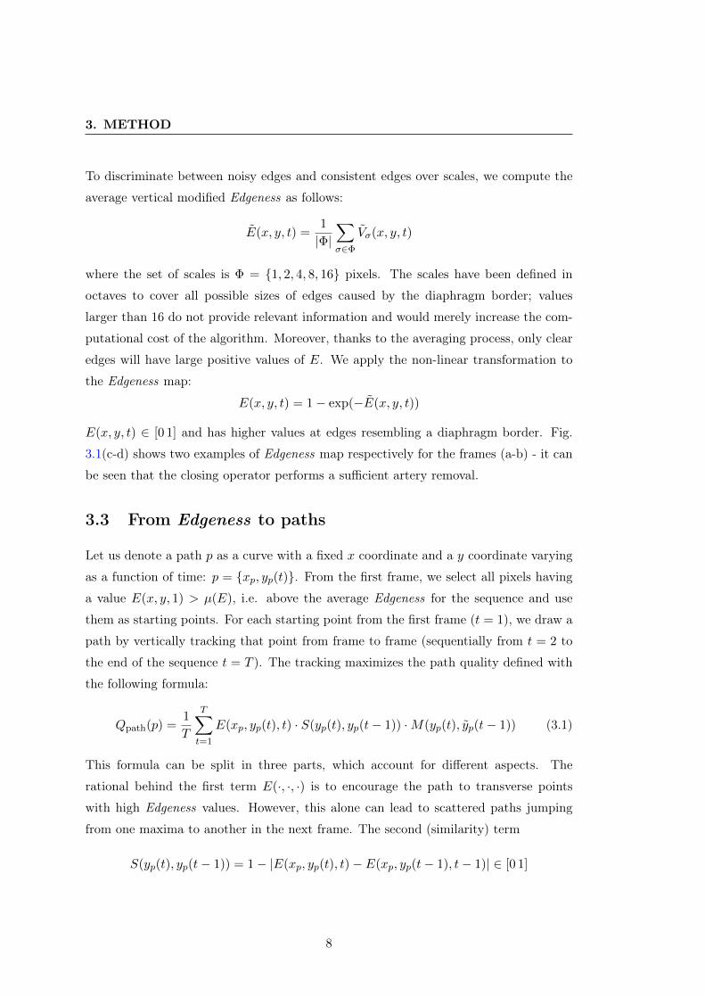
To discriminate between noisy edges and consistent edges over scales, we compute the
average vertical modified Edgeness as follows:
E(x, y, t) =1
|Φ|∑
σ∈Φ
Vσ(x, y, t)
where the set of scales is Φ = {1, 2, 4, 8, 16} pixels. The scales have been defined in
octaves to cover all possible sizes of edges caused by the diaphragm border; values
larger than 16 do not provide relevant information and would merely increase the com-
putational cost of the algorithm. Moreover, thanks to the averaging process, only clear
edges will have large positive values of E. We apply the non-linear transformation to
the Edgeness map:
E(x, y, t) = 1 − exp(−E(x, y, t))
E(x, y, t) ∈ [0 1] and has higher values at edges resembling a diaphragm border. Fig.
3.1(c-d) shows two examples of Edgeness map respectively for the frames (a-b) - it can
be seen that the closing operator performs a sufficient artery removal.
3.3 From Edgeness to paths
Let us denote a path p as a curve with a fixed x coordinate and a y coordinate varying
as a function of time: p = {xp, yp(t)}. From the first frame, we select all pixels having
a value E(x, y, 1) > µ(E), i.e. above the average Edgeness for the sequence and use
them as starting points. For each starting point from the first frame (t = 1), we draw a
path by vertically tracking that point from frame to frame (sequentially from t = 2 to
the end of the sequence t = T ). The tracking maximizes the path quality defined with
the following formula:
Qpath(p) =1
T
T∑
t=1
E(xp, yp(t), t) · S(yp(t), yp(t − 1)) · M(yp(t), yp(t − 1)) (3.1)
This formula can be split in three parts, which account for different aspects. The
rational behind the first term E(·, ·, ·) is to encourage the path to transverse points
with high Edgeness values. However, this alone can lead to scattered paths jumping
from one maxima to another in the next frame. The second (similarity) term
S(yp(t), yp(t − 1)) = 1 − |E(xp, yp(t), t) − E(xp, yp(t − 1), t − 1)| ∈ [0 1]
8

3.3 From Edgeness to paths
imposes minimal Edgeness value variation between consecutive path points. The third
term
M(yp(t), yp(t)) = e− (yp(t)−yp(t))2
2σ2M
has been designed to add a smoothness criterion to the path construction. Here yp(t) is
the expected value for the time location t, based on the linear approximation of previous
values1:
yp(t) = 2yp(t − 1) − yp(t − 2)
Basically, the use of a Gaussian (with its σM parameter) centered around the expected
location yp(t) adds a constraint, so that paths are restricted from changing their trajec-
tories in a way that does not resemble a continuous movement. All of the three terms
are bounded in [0 1], so that their product ensures that only points fulfilling the three
criteria at once are selected. The smoothness parameter σM has been defined by cross-
validation. Fig. 3.2 shows the plotted error for different σM values using a training
set of 9 images. As it can be seen σM = 5 [pixels] is the optimal choice. Changing the
linear model for predicting yp(t) with a second order degree polynomial resulted in lower
performance. Since the proposed path building is based on local decisions maximizing
5 10 15 20 25 30 35 40 45 50 55
101.4
101.5
101.6
101.7
101.8
101.9
σM
Housdorff
dis
tance
5 10 15 20 25 30 35 40 45 50 5510
0
101
σM
MM
D
Hausdorff distance MMD
Figure 3.2: Average distances over the training set when varying σM .
equation (3.1), we allow the construction of multiple paths given an x. However, to
avoid path proliferation, if two paths collide, only the one with higher path quality is
retained, so that at the end of the process we have a set of non-intersecting continuous
1We make the ’zeroth’ and the ’minus first’ frames the same as the first one.
9
3. METHOD
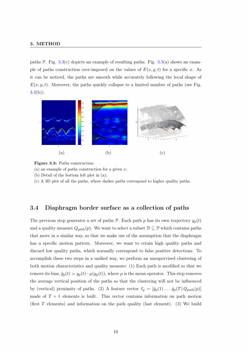
paths P. Fig. 3.3(c) depicts an example of resulting paths. Fig. 3.3(a) shows an exam-
ple of paths construction over-imposed on the values of E(x, y, t) for a specific x. As
it can be noticed, the paths are smooth while accurately following the local shape of
E(x, y, t). Moreover, the paths quickly collapse to a limited number of paths (see Fig.
3.3(b)).
t
y
0
0.1
0.2
0.3
0.4
0.5
0.6
0.7
0.8
0.9
t
y
(a) (b) (c)
Figure 3.3: Paths construction:(a) an example of paths construction for a given x;(b) Detail of the bottom left plot in (a);(c) A 3D plot of all the paths, where darker paths correspond to higher quality paths.
3.4 Diaphragm border surface as a collection of paths
The previous step generates a set of paths P. Each path p has its own trajectory yp(t)
and a quality measure Qpath(p). We want to select a subset D ⊆ P which contains paths
that move in a similar way, so that we make use of the assumption that the diaphragm
has a specific motion pattern. Moreover, we want to retain high quality paths and
discard low quality paths, which normally correspond to false positive detections. To
accomplish these two steps in a unified way, we perform an unsupervised clustering of
both motion characteristics and quality measure: (1) Each path is modified so that we
remove its bias, yp(t) = yp(t)−µ(yp(t)), where µ is the mean operator. This step removes
the average vertical position of the paths so that the clustering will not be influenced
by (vertical) proximity of paths. (2) A feature vector vp = [yp(1) . . . yp(T ) Qpath(p)]
made of T + 1 elements is built. This vector contains information on path motion
(first T elements) and information on the path quality (last element). (3) We build
10

3.4 Diaphragm border surface as a collection of paths
a matrix V where each row contains a feature vector vp for each path in P. Since
vertical positions and quality measure are incommensurable we need to normalize V
such that every column has zero mean and unitary standard deviation. (4) We apply
an unsupervised k-means∗ clustering; the cluster with the highest mean quality is the
one which most probably defines the diaphragm border as a collection of paths. The use
of unsupervised clustering is the most suited way to group paths into a consistent result
since the actual diaphragm motion is unpredictable: a sequence can be acquired while
the patient is holding the breath, or the patient can have irregular breathing pattern.
On the other way, k-means requires the definition of the number of clusters, which we
set to three. The rational behind this setting is to allow the clustering to find one
cluster for the diaphragm, one cluster for noisy low quality paths and a third cluster
which has a motion pattern that is a mixture of the diaphragm and cardiac patterns.
This latter case has been considered since the morphological operator is not able to
eliminate non-tubular structures that move according to the cardiac cycle. Fig. 3.4(a)
shows the result of clustering for the case in Fig. 3.3(c); different clusters are depicted
in different colors.
(a) (b)
Figure 3.4: (a) The paths of Fig. 3.3(c) colored in accordance to their clusters; the greencluster is the selected one. (b) The resulting surface after fitting the polynomial functionto all the sequence frames.
∗ Since the k-means is based on random centroids initialization, and it is not computational costly,we perform 100 trials keeping the solution with the lowest objective function.
11
3. METHOD
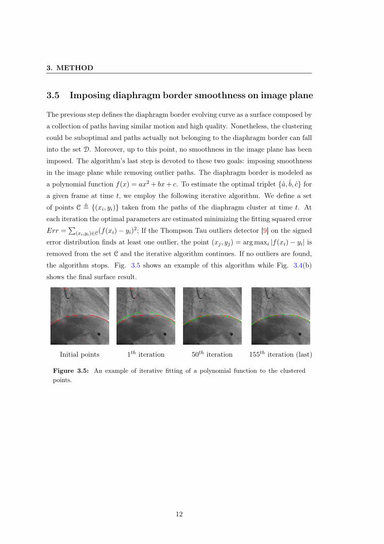
3.5 Imposing diaphragm border smoothness on image plane
The previous step defines the diaphragm border evolving curve as a surface composed by
a collection of paths having similar motion and high quality. Nonetheless, the clustering
could be suboptimal and paths actually not belonging to the diaphragm border can fall
into the set D. Moreover, up to this point, no smoothness in the image plane has been
imposed. The algorithm’s last step is devoted to these two goals: imposing smoothness
in the image plane while removing outlier paths. The diaphragm border is modeled as
a polynomial function f(x) = ax2 + bx + c. To estimate the optimal triplet {a, b, c} for
a given frame at time t, we employ the following iterative algorithm. We define a set
of points C , {(xi, yi)} taken from the paths of the diaphragm cluster at time t. At
each iteration the optimal parameters are estimated minimizing the fitting squared error
Err =∑
(xi,yi)∈C(f(xi) − yi)2; If the Thompson Tau outliers detector [9] on the signed
error distribution finds at least one outlier, the point (xj , yj) = arg maxi |f(xi) − yi| is
removed from the set C and the iterative algorithm continues. If no outliers are found,
the algorithm stops. Fig. 3.5 shows an example of this algorithm while Fig. 3.4(b)
shows the final surface result.
Initial points 1th iteration 50th iteration 155th iteration (last)
Figure 3.5: An example of iterative fitting of a polynomial function to the clusteredpoints.
12
4
Validation
4.1 Validation framework
Material: We defined a validation set of 16 frames taken from 11 sequences (11 pa-
tients). The diaphragm border in each frame has been marked blindly by two experts.
All sequences have been acquired using a Philips Allura Xper FD20, at 12.5 fps and
with an image resolution of 0.34×0.34 mm. The C-arm position varies from -41◦ to 97◦
for the primary angle and from -17◦ to 33◦ for the secondary angle.
Methods: We compare our proposed method with the diaphragm detection algorithm
described in [1]. We also compute the inter-observer variability between the two ground
truth annotations. Moreover, we also provide intermediate evaluations of algorithms.
Validation protocol: Let GT be the set of points forming the ground truth curve
and P be the set of points predicted by a given method. We use two different measures
to validate each prediction against the ground truths: (1) The Hausdorff distance [10]
is the distance between the two most faraway points from the two sets of points. This
measure is very sensitive to predicted points laying far from the ground truth points
but gives little information about the overall precision of the prediction, thus making it
useful in measuring robustness. (2) The Mean Minimal Distance
MMD(P, GT ) =1
|P |∑
i∈P
minj∈GT
||(xPi , yP
i ) − (xGTj , yGT
j )||
13

4. VALIDATION
on the other hand, provides information about the overall precision of the predicted
result. It has to be noted that the MMD is not symmetric.
4.2 Results
Table 4.1 shows the error results using the Hausdorff and the MMD distances for the
following cases (one for each row): inter-observer variability; the method in [1] before
and after the application of the snake; our method prior to the clustering (Our-PC),
prior to the curve fitting (Our-PF) and the final result (Our). For each distance, tables
report its mean, standard deviation, minimum and maximum values.
An interesting fact is that the use of snakes, as expected, can help the method in
[1] to improve the results but in a very limited extent. Regarding our method, it can
be noticed that each step improves the results. Once the paths are built, before the
clustering, the method is limited in the fact that the sequence is analyzed mainly in its
temporal dimension, so that a large number of incorrect paths can be generated. The
clustering step selects a set of paths that potentially represent the diaphragm border;
this decreases consistently the MMD error (three times), but is not able to reduce the
Hausdorff distance since erroneous paths far from the solution could be maintained.
The polynomial fitting ensures a consistent solution imposing smoothness in the image
domain and, at the same time, rejects erroneous paths thanks to the outlier detection;
this results in a huge improvement in both the Hausdorff and MMD distances (more
than one order of magnitude).
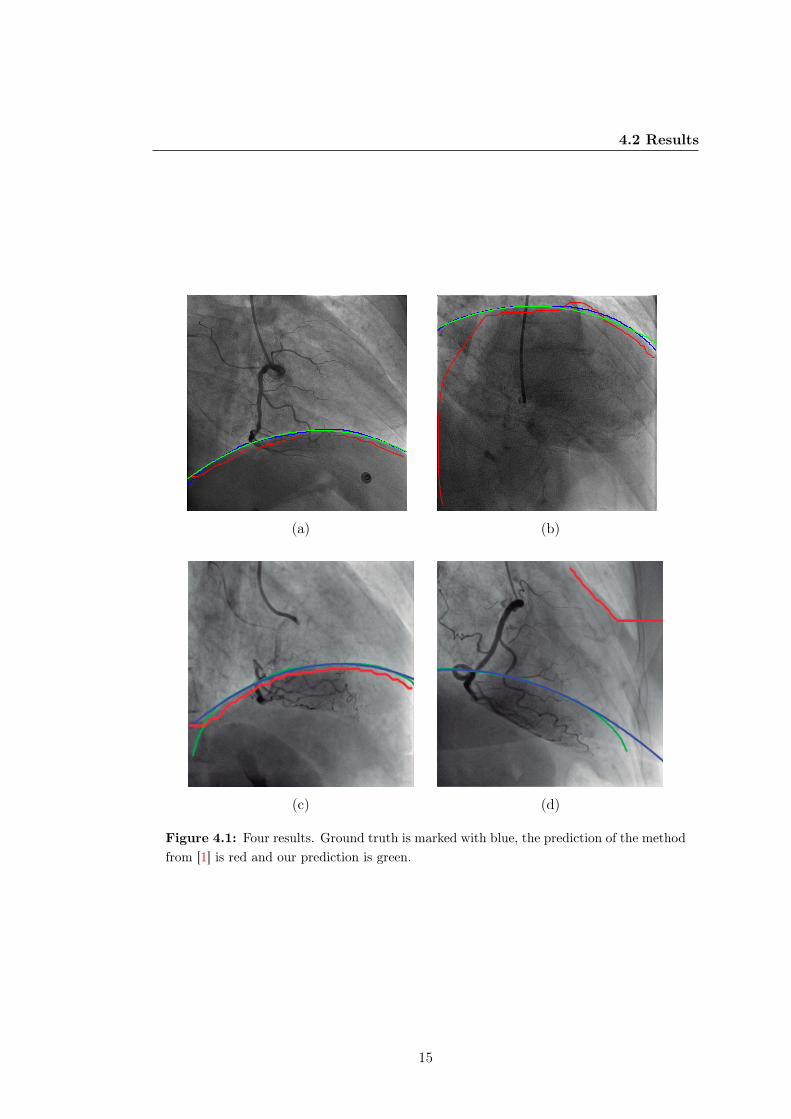
Results confirm that taking advantage of temporal and spatial properties of the di-
aphragm in a unified way produces far better results than relying only on frame based
appearance. Fig. 4.1 shows four results:
Case (a) Both methods detect the diaphragm robustly, while our method (in green)
shows a higher accuracy.
Case (b) A more difficult case - the method in [1] fails to detect a segment of the
diaphragm border.
Cases (c) and (d) show that sometimes the diaphragm parabolic model might be
too simple.
14
4.2 Results
(a) (b)
(c) (d)
Figure 4.1: Four results. Ground truth is marked with blue, the prediction of the methodfrom [1] is red and our prediction is green.
15

4. VALIDATION
Hausdorff distance MMDAvg±Std min max Avg±Std min max
O1 vs O2 25.82±22.75 4 86.33 2.03±2.07 0.78 7.84O2 vs O1 25.82±22.75 4 86.33 1.41±0.66 0.75 3.35
[1] (no snakes) 83.36±124.37 22.14 429.17 32.09±50.65 14.24 233.49[1] 84.71±120.73 17.03 407.12 28.04±54.42 10.71 234.17
Our-PC 364±48.5 287 440 132±19.7 108 185Our-PF 302±58.1 188 385 43.7±25.5 16.7 85.0
Our 29.1±23.5 5.4 97.2 3.00±1.81 1.34 9.55
Table 4.1: Quantitative results. All measures are in pixels
16

5
Discussion
The proposed method shows some very good results, both in robustness and precision.
While demonstrating potential it also reveals some of the challenging key points that
still need to be solved before the ideas here reach trustful clinical practice.
Parabola fitting: It is not always the case that the diaphragm border has the shape
of a parabola (fixed in rotation) - Fig. 4.1 (c) and (d). It could be that the polynomial
model for the diaphragm border is too simple and that raises questions about balance
between robustness and precision.
More than one diaphragm borders: It may be the case when the diaphragm bor-
ders are more than one. Biologically the diaphragms are two and in some projections
both of them are present.
17

5. DISCUSSION
18

6
Conclusions
In this thesis we proposed an algorithm for the robust and accurate detection of the
diaphragm border in X-ray angiographies plus a validation methodology for quantitative
performance evaluation. Results show that the proposed method is both robust and
accurate. However, further investigation on how to deal with highly challenging cases
is required. As future works, we want to:
(1) Increase the validation dataset
(2) Propose a digital diaphragm removal algorithm based on the detection proposed
herein.
(3) Apply the method in an automatic tool for estimating the myocardial perfusion
level.
The method described in this thesis has been submitted as a paper to the International
Workshop on Statistical Atlases and Computational Models of the Heart, which is part
of MICCAI 2012 conference.
19

6. CONCLUSIONS
20
References
[1] A. Condurache, T. Aach, K. Eck, J. Bredno, and T. Stehle, “Fast and robust
diaphragm detection and tracking in cardiac x-ray projection images,” in Spie MI,
vol. 5747, pp. 1766–1775, 2005. vii, 1, 3, 6, 13, 14, 15, 16
[2] A. Condurache, T. Aach, A. Kaiser, and P. Radke, “User-defined ROI tracking of
the myocardial blush grade,” in 7th IEEE SSIAI, (Denver, CO), pp. 66–70, IEEE
Computer Society, March 28-30 2006. 1
[3] D. Gil, O. Rodriguez-Leor, P. Radeva, and J. Mauri, “Myocardial perfusion char-
acterization from contrast angiography spectral distribution,” IEEE TMI, vol. 27,
no. 5, pp. 641–649, 2008. 1
[4] J. Liénard and R. Vaillant, “Quantitative tool for the assessment of myocardial
perfusion during x-ray angiographic procedures,” in Proceedings of the 5th ICFIMH,
FIMH ’09, (Berlin, Heidelberg), pp. 124–133, Springer-Verlag, 2009. 1
[5] C. Gatta, J. D. G. Valencia, F. Ciompi, O. Rodriguez-Leor, and P. Radeva, “Toward
robust myocardial blush grade estimation in contrast angiography,” in IbPRIA,
pp. 249–256, 2009. 1, 2
[6] R. Duda and P. Hart, “Use of the hough transformation to detect lines and curves
in pictures,” Tech. Rep. 36, AI Center, SRI International, 333 Ravenswood Ave,
Menlo Park, CA 94025, Apr 1971. SRI Project 8259 Comm. ACM, Vol 15, No. 1.
3
[7] N. Funabashi, Y. Kobayashi, M. Perlroth, and G. Rubin, “Coronary artery: quanti-
tative evaluation of normal diameter determined with electron-beam ct compared
21
REFERENCES
with cine coronary angiography initial experience.,” Radiology, vol. 226, no. 1,
pp. 263–71, 2003. 6
[8] T. Lindeberg, “Principle for automatic scale selection,” tech. rep., RIT, 1998. 6
[9] T. R., “A note on restricted maximum likelihood estimation with an alternative
outlier model,” Journal of the Royal Statistical Society. Series B, vol. 47, pp. 53–
55, 1985. 12
[10] J. Henrikson, “Completeness and total boundedness of the hausdorff metric.,” MIT
Undergraduate Journal of Mathematics, vol. 1, pp. 69–80, 1999. 13
22