Robust adaptive beamforming using worst-case …vorobyov/RobBeamformer.pdf · IEEE TRANSACTIONS ON...

IEEE TRANSACTIONS ON SIGNAL PROCESSING, VOL. 51, NO. 2, FEBRUARY 2003 313

Robust Adaptive Beamforming Using Worst-CasePerformance Optimization: A Solution to the Signal

Mismatch ProblemSergiy A. Vorobyov, Member, IEEE, Alex B. Gershman, Senior Member, IEEE, and Zhi-Quan Luo, Member, IEEE

Abstract—Adaptive beamforming methods are known todegrade if some of underlying assumptions on the environment,sources, or sensor array become violated. In particular, if thedesired signal is present in training snapshots, the adaptivearray performance may be quite sensitive even to slight mis-matches between the presumed and actual signal steering vectors(spatial signatures). Such mismatches can occur as a result ofenvironmental nonstationarities, look direction errors, imperfectarray calibration, distorted antenna shape, as well as distortionscaused by medium inhomogeneities, near–far mismatch, sourcespreading, and local scattering. The similar type of performancedegradation can occur when the signal steering vector is knownexactly but the training sample size is small.

In this paper, we develop a new approach to robust adaptivebeamforming in the presence of an arbitrary unknown signalsteering vector mismatch. Our approach is based on the opti-mization of worst-case performance. It turns out that the naturalformulation of this adaptive beamforming problem involvesminimization of a quadratic function subject to infinitely manynonconvex quadratic constraints. We show that this (originallyintractable) problem can be reformulated in a convex form as theso-called second-order cone (SOC) program and solved efficiently(in polynomial time) using the well-established interior pointmethod. It is also shown that the proposed technique can be in-terpreted in terms of diagonal loading where the optimal value ofthe diagonal loading factor is computed based on the known levelof uncertainty of the signal steering vector. Computer simulationswith several frequently encountered types of signal steering vectormismatches show better performance of our robust beamformeras compared with existing adaptive beamforming algorithms.

Index Terms—Optimal diagonal loading, robust adaptivebeamforming, second-order cone programming, signal mismatchproblem, worst-case performance optimization.

I. INTRODUCTION

I N recent decades, adaptive beamforming has been widelyused in wireless communications, microphone array speech

processing, radar, sonar, medical imaging, radio astronomy,and other areas. A traditional approach to the design of adaptivebeamformers assumes that the desired signal components are

Manuscript received October 17, 2001; revised October 10, 2002. Thiswork was supported in part by the Natural Sciences and Engineering ResearchCouncil (NSERC) of Canada, Communications and Information TechnologyOntario (CITO), Premier’s Research Excellence Award Program of theMinistry of Energy, Science, and Technology (MEST) of Ontario, CanadaResearch Chairs Program, and Wolfgang Paul Award Program of the Alexandervon Humboldt Foundation. The associate editor coordinating the review of thispaper and approving it for publication was Dr. Rick S. Blum.

The authors are with the Department of Electrical and Computer Engineering,McMaster University, Hamilton, ON, L8S 4K1 Canada.

Digital Object Identifier 10.1109/TSP.2002.806865

not present in training data [1]. In this case, several rapidlyconverging techniques have been developed [1]–[5] that are ap-plicable to problems with small training sample size. Althoughthe assumption of signal-free training snapshots may be truein some areas (such as radar), there are numerous applicationswhere the observations are always “contaminated” by the signalcomponent. Such applications, for example, include mobilecommunications, passive source location, microphone arrayspeech processing, medical imaging, and radio astronomy. It iswell known that even in the ideal case where the signal steeringvector is exactly known, the presence of the signal of interestin training data cell may dramatically reduce the convergencerates of adaptive beamforming algorithms as compared with thesignal-free training data case [6]. This may cause a substantialdegradation of the performance of adaptive beamformingtechniques in situations of small training sample size.

When adaptive arrays are applied to practical problems, theperformance degradation of adaptive beamforming techniquesmay become even more pronounced than in the aforementionedideal case because some of underlying assumptions on the envi-ronment, sources, or sensor array can be violated and this maycause a mismatch between the nominal (presumed) and actualsignal steering vectors. Adaptive array techniques are known tobe very sensitive even to slight mismatches of such type that caneasily occur in practical situations as a consequence of look di-rection and signal pointing errors [7], [8] or imperfect array cal-ibration and distorted antenna shape [9]. Other common causesof model mismatch include array manifold mismodeling due tosource wavefront distortions resulting from environmental inho-mogeneities [10], [11], near–far problem [12], source spreadingand local scattering [13]–[16], as well as other effects [17]. Insuch cases, robust approaches to adaptive beamforming are re-quired [17]–[19].

There are several existing approaches to robust adaptivebeamforming. The most common is the so-called linearlyconstrained minimum variance (LCMV) beamformer, whichprovides robustness against uncertainty in the signal lookdirection. Recently, several other techniques addressing thistype of mismatch have been developed (see [19] and referencestherein). However, the applicability of these techniques islimited by scenarios with look direction mismatches only. Ifany other types of steering vector mismatch become dominant(e.g., mismatches due to array perturbations, array manifoldmismodeling, wavefront distortions, or source local scattering),these methods cannot be expected to provide sufficient robust-ness improvements [17].

1053-587X/03$17.00 © 2003 IEEE

314 IEEE TRANSACTIONS ON SIGNAL PROCESSING, VOL. 51, NO. 2, FEBRUARY 2003

Several other approaches are known to be able to partly over-come the problem of arbitrary steering vector mismatches. Themost popular of them are the quadratically constrained beam-former (whose implementation is based on the so-calleddiag-onal loadingof the sample covariance matrix [4], [18], [20])and the eigenspace-based beamformer [6], [21]. However, themain shortcoming of the former approach is that it is not clearhow to obtain the optimal value of the diagonal loading factorbased on the known level of uncertainty of the signal steeringvector, whereas the latter approach is essentially ineffective atlow signal-to-noise ratios (SNRs) and when the dimension ofthe signal-plus-interference subspace is high.1 This, unfortu-nately, makes it difficult to apply the eigenspace-based beam-former to wireless communications where the dimension of thesignal-plus-interference subspace may be uncertain and rela-tively high due to the effects of signal local scattering [13]–[16].

In this paper (also see [22]–[24]), we develop a new powerfulapproach to robust adaptive beamforming in the presence ofan arbitrary unknown steering vector mismatch. Our approachis based on the optimization of worst-case performance. Itturns out that the natural formulation of this problem involvesminimization of a quadratic function subject to infinitely manynonconvex quadratic constraints and therefore is NP-hard2 tosolve. However, we show that this robust adaptive beamformingproblem can be reformulated as a convex second-order cone(SOC) program and solved efficiently (in polynomial time)via the well-established interior point method (see [27]–[29]).This result is somewhat surprising from the optimizationtheory standpoint and is based on a procedure that transformsa semi-infinite nonconvex quadratically constrained homo-geneous quadratic minimization problem to a convex SOCprogram. We show that our beamformer can be interpreted as adiagonal loading approach3 in which the optimal value of thediagonal loading factor is computed based on the known upperbound on the norm of the signal steering vector mismatch.

Computer simulations with several frequently encounteredtypes of signal steering vector mismatches show a visible perfor-mance gain of the proposed beamformer over other traditionaland robust adaptive beamforming techniques.

Our paper is organized as follows. Some background of adap-tive beamforming is presented in Section II, where several pop-ular robust adaptive beamforming techniques are overviewed. InSection III, we first describe a new formulation of robust adap-tive beamforming based on the optimization of worst-case per-formance. Then, we establish the diagonal loading based inter-pretation of our robust adaptive beamforming problem and con-vert it to a convex SOC problem that can be efficiently solvedusing the well-established interior point algorithms. Section IVpresents our simulation results where the performance of theproposed method is compared with the existing algorithms insituations with different types of the signal steering vector mis-match. Section V contains our concluding remarks.

1Additionally, this dimension must be exactly known in this technique.2In optimization theory, NP-hard problems represent a class of extremely dif-

ficult problems that have no known polynomial-time solutions [25].3Very recently, another robust worst-case optimization-based beamformer

(which also belongs to the class of diagonal loading techniques) has beenindependently formulated; see [26].

II. BACKGROUND

The output of a narrowband beamformer is given by

where is the time index,is the complex vector of array observations,

is the complex vector ofbeamformer weights, is the number of array sensors, and

and stand for the transpose and Hermitian transpose,respectively. The observation (training snapshot) vector isgiven by

(1)

where , , and are the desired signal, interference,and noise components, respectively. Here, is the signalwaveform, and is the signal steering vector. The weight vectorcan be found from the maximum of the signal-to-interference-plus-noise ratio (SINR) [5]

SINR (2)

where

(3)

is the interference-plus-noise covariance matrix, andis the signal power. It is easy to find the solution for the

weight vector by maintaining a distortionless response towardthe desired signal and minimizing the output interference-plus-noise power [5]. Hence, the maximization of (2) is equivalent to[5]

subject to (4)

From (4), the following well-known solution can be found forthe optimal weight vector [5]:

(5)

where is the normalization constant thatdoes not affect the output SINR (2) and, therefore, will beomitted in the interest of brevity. The solution (5) is commonlyreferred to as the minimum variance distortionless response(MVDR) beamformer [5], [30].

In practical applications, the exact interference-plus-noise co-variance matrix is unavailable. Therefore, the sample co-variance matrix

(6)

is used instead of (3) (see [1]). Here,is the number of trainingsnapshots (also termed thetraining sample size). In this case, (4)should be rewritten as

subject to (7)

VOROBYOV et al.: ROBUST ADAPTIVE BEAMFORMING USING WORST-CASE PERFORMANCE OPTIMIZATION 315

The solution to this problem is commonly referred to as thesample matrix inversion (SMI) algorithm, whose weight vector(after omitting the immaterial constant ) isgiven by [1]

(8)

When the signal component is present in the training data cell(cf. (1)), the use of the sample covariance matrix (6) in placeof the true interference-plus-noise covariance matrix (3) affectsthe performance of the SMI algorithm dramatically [6]. It is wellknown since the classic paper [1] that in the case of signal-freetraining samples, the use of weight vector (8) provides rapidconvergence of the output SINR to its optimal value

SINR (9)

so that the average performance losses relative to (9) are lessthan 3 dB if . However, this is no longer true if thetraining snapshots are “contaminated” by the signal component.It was shown in [6] that in the latter case the convergence to (9)becomes much slower and generally requires .

Another essential shortcoming of the SMI algorithm is thatit does not provide sufficient robustness against a mismatch be-tween the presumed and actual signal steering vectorsand .Here, denotes the actual steering vector that characterizes thespatial signature of the signal. In the mismatched case

(10)

where is an unknown complex vector that describes the effectof steering vector distortions. As a result, the SMI beamformertends to “interpret” the signal components in array observationsas an interference and tries to suppress these components bymeans of adaptive nulling instead of maintaining distortionlessresponse toward (see [6] and [17]).

In the mismatched case, (2) and (9) should be rewritten as

SINR (11)

and

SINR (12)

respectively. Several robust modifications of the SMI algorithmhave been developed to improve its performance in the above-mentioned cases with signal steering vector mismatches andsmall training sample size. One of the most popular robust ap-proaches is the so-called loaded SMI (LSMI) algorithm, whichis based on the diagonal loading of the sample covariance matrix[4], [18]. The essence of this approach is to replace the conven-tional sample covariance matrix by the so-called diagonallyloaded covariance matrix

(13)

in the SMI algorithm (8). Here, is a diagonal loading factor,and is the identity matrix. Using (13), we can write the LSMIweight vector in the following form [4]:

(14)

The main problem of the LSMI method is how to chose thediagonal loading factor. Cox et al. [18] proposed to use theso-calledwhite noise gain constraintto obtain reasonable valuesof this parameter. Unfortunately, it is not clear how to relate theparameters of the white noise gain constraint and the level ofuncertainty of the signal steering vector. Furthermore, the rela-tionship between the diagonal loading factor and the parametersof the white noise gain constraint is not simple, and to satisfy thisconstraint, a multistep iterative procedure is required to adjustthe diagonal loading factor [18]. Each step of this iterative pro-cedure involves an update of the inverse of the diagonally loadedcovariance matrix, and as a result, the total computational com-plexity of adaptive beamforming with the white noise gain con-straint may be higher than that of the SMI algorithm. Becauseof this, the diagonal loading factor is usually chosen in a moread hocway, typically about 10 , where is the noise powerin a single sensor.

Another popular approach to robust adaptive beamformingin the general case of an arbitrary mismatch is the so-calledeigenspace-based beamformer [6], [21] whose key idea is to use,instead of the presumed steering vector, the projection ofonto the sample signal-plus-interference subspace. The eigen-decomposition of (6) yields

where the matrix contains the signal-plus-interference subspace eigenvectors of, and the diagonalmatrix contains the corresponding eigen-values of . Similarly, the matrix containsthe noise-subspace eigenvectors of, whereas thediagonal matrix is built from the cor-responding eigenvalues. Here,is the number of interferingsources (or, mathematically, the rank of the interference sub-space), which is assumed to be known. The weight vector of theeigenspace-based beamformer is given by

(15)

where

(16)

are the projected steering vector and the orthogonal projectionmatrix onto the signal-plus-interference subspace, respectively.Inserting (16) into (15), the latter equation can be rewritten as

(17)

The eigenspace-based beamformer is known to be one of themost powerful robust techniques applicable to arbitrary steeringvector mismatch case [21]. However, an essential shortcomingof this approach is that it is limited to high SNR cases be-cause at low SNR the estimation of the projection matrix ontothe signal-plus-interference subspace breaks down because of ahigh probability of subspace swaps [31], [32]. Moreover, theeigenspace-based beamformer is efficient only if the dimen-sion of the signal-plus-interference subspace is low and knownexactly. This makes it difficult to apply the eigenspace-basedbeamformer to wireless communications where the dimension


of the signal-plus-interference subspace may be uncertain andrelatively high due to the effects of source scattering [13]–[16].

III. N EW APPROACH TOROBUSTBEAMFORMING

In this section, we develop a new adaptive beamformer thatis robust against an arbitrary signal steering vector mismatchand small training sample size. Our approach is based on theworst-case performance optimization. We begin with the formu-lation of the robust adaptive beamforming problem and then de-velop a convex optimization-based implementation of our adap-tive beamformer using SOC programming.

A. Formulation

We assume that in practical applications, the norm of thesteering vector distortion can be bounded4 [33] by someknown constant :

(18)

Then, the actual signal steering vector belongs to the set

(19)

Indeed, if , then, according to (10), . Since canbe any vector in (19), we impose a constraint that for all vectorsthat belong to , the absolute value5 of the array responseshould not be smaller than one, i.e.,

for all (20)

Using (20), the robust formulation of adaptive beamformer canbe written as the following constrained minimization problem:

subject to for all (21)

Note that (21) represents a modified version of (7). Themain modification of (7) is that instead of requiring fixeddistortionless response toward the single steering vector, in(21), such distortionless response is maintained by means ofinequality constraints6 for a continuum of all possible steeringvectors given by the set . Hence, the constraints in (21)guarantee that the distortionless response will be maintained intheworst case, i.e., for the particular vector that correspondsto the smallest value of . Therefore, such a design shouldimprove the beamformer robustness against signal steeringvector mismatches that satisfy (18) because in this case, themismatched vector belongs to the set .

For each choice of , the conditionrepresents a nonlinear andnonconvexconstraint on . Sincethere is an infinite number of vectorsin , there is an in-finite number of such constraints. Hence, (21) is a semi-infinite

4Note that this corresponds to a much more general class of mismatches thanconsidered in [34], where the bounds on the mismatch vector itself are usedrather than that on the norm of this vector.

5An important issue that is beyond our present consideration is how to controlthe phase of the beam response. This issue may be critical when, for example,adaptive beamforming has to be performed over frequency subbands whose out-puts must be coherently integrated.

6Constraints in the form of inequality (sometimes referred to assoft con-straints) are used in other adaptive beamforming techniques as well [35]–[37].

nonconvex quadratic program. It is well known that the gen-eral nonconvex quadratically constrained quadratic program-ming problem is NP-hard and, thus, intractable. However, aswe will show next, due to the special structure of the objectivefunction and the constraints, the problem (21) can be reformu-lated, surprisingly, as a convex SOC program and, thus, solvedefficiently (in polynomial time) via the well established interiorpoint method.

Let us first convert the semi-infinite nonconvex constraints toa single constraint that corresponds to the worst-case constraintfrom (20). In particular, (21) can be equivalently described as

subject to (22)

According to (19), we can rewrite the constraint of (22) as

where the set is defined as

Applying the triangle and Cauchy–Schwarz inequalities alongwith the inequality , we have that

(23)

Moreover, it is easy to verify that

(24)

if is small enough (i.e., if ) and if

where

angle

Note that we require that , as otherwise, thewhite noise gain of the robust beamformer may be insufficient[18].

Then, combining (23) and (24), we conclude that

and therefore, the semi-infinite nonconvex quadratically con-strained problem (22) can be written as the following quadraticminimization problem with asinglenonlinear constraint:

subject to (25)

The nonlinear constraint in (25) is still nonconvex due to the ab-solute value operation on the left-hand side. An important ob-servation is that the cost function in (25) isunchangedwhenundergoes an arbitrary phase rotation. Therefore, ifis an op-timal solution to (25), we can always rotate, without affectingthe objective function value, the phase ofso that is real.Thus, we can, without any loss of generality, choosesuch that

Re (26)

Im (27)


Using this observation and employing (26) and (27) as addi-tional constraints, the constraint in (25) can be written as

(28)

From (28) along with (27), it follows that Re . Sincethe constraint (26) is taken into account by (27) and (28), thereis no need to add this constraint to the minimization problem(25). Therefore, this problem can be rewritten as

subject to

Im (29)

Note that the problem (29) has much simpler formulation than(21) and isconvex.

B. Relationship to the LSMI Beamformer

To clarify the problem (29) more, note that the constraint in(22) is equivalent to

(30)

or, in other words, (29) corresponds to maximization of theworst-case output SINR. The equivalence of the equality con-straint (30) and the inequality constraint in (22) can be easilyproved by contradiction as follows. If they are not equivalent toeach other, then the minimum of the objective function in (22)is achieved when . However, re-placing with , we can decrease the objective function

by the factor of , whereas the constraint in (22)will be still satisfied. This contradicts the original statement thatthe objective function is minimized when . Therefore, theminimum of the objective function is achieved at , andthis proves that the inequality constraint in (29) is equivalent tothe equality constraint . Therefore, isreal-valued and positive, and the constraint Im canbe ignored. Using these facts, we can rewrite the problem (29)as

subject to (31)

The solution to (31) can be found by minimizing the function

where is a Lagrange multiplier. Taking the gradient ofand equating it to zero gives

Applying the matrix inversion lemma to the latter equation, weobtain

(32)

which shows that the proposed robust beamformer belongs tothe class of diagonal loading techniques.

Note, however, that it is not easy to use (32) directly for com-puting the optimal weight vector because it is not clear how to

obtain the Lagrange multiplier in a closed form [26]. There-fore, to solve (29), an efficient SOC programming-based ap-proach is developed in the next section.

C. SOC Implementation

The next step involves developing a SOC formulation of (29).Note that although we have shown in the previous section thatthe inequality constraint in (29) can be replaced by equality, wewill use this constraint in its original inequality form, which issuitable for the SOC implementation.

First of all, we convert the quadratic objective function of (29)to a linear one. Let

(33)

be the Cholesky factorization of. Using (33), we can convertthe objective function of (29) into

(34)

Apparently, minimizing is equivalent to minimizing (34).Hence, introducing a new scalar non-negative variableand anew constraint , we can convert (29) into the fol-lowing problem:

subject to

Im (35)

To facilitate the solution of (35), we need to convert it to a real-valued form. Introducing

Re Im

Re Im

Im Re

Re ImIm Re

we rewrite (35) in terms of real-valued vectors and matrices as

subject to

(36)

Let us define

where is the vector of zeros of a conformable dimension. Withthese notations, (36) can be further transformed to the following


canonicaldual form7 of the SOC programming problem (whichis equivalent to (8) in [29]):

subject to

SOC SOC (37)

where is the vector of variables, SOC is the second-ordercone of the dimension , which corresponds to thethinequality constraint in (36) ( ,2), and {0} is the so-calledzero cone that determines the hyperplane due to the equalityconstraint . More specifically

SOC

where

Note that after solving the optimization problem (37), the onlyparameters of interest in the vector of variablesare given by itssubvector . The resulting weight vector of our robust adaptivebeamformer is given by

(38)

In summary, we converted the robust beamforming problem(21) to the canonical SOC problem (37). Note that althoughthese problems are mathematically equivalent, the originalproblem (21) is computationally intractable, whereas the SOCproblem (37) can be easily solved using standard and highlyefficient interior point method software tools, e.g., [29]. Forexample, using the primal-dual potential reduction method[27], the complexity of our beamformer is per iteration[28], and the algorithm converges typically in less than teniterations (a well-known and accepted fact in the optimizationcommunity). Therefore, the overall complexity of our beam-former is . This is the same order of complexity asthat of the SMI algorithm. However, the SMI algorithm has acomputational advantage in theon-line mode, where the RLSalgorithm can be used to update the SMI beamformer weightswith the computational complexity per updating step.The weight vector of our beamformer cannot be easily updatedbut has to be recomputed in each step.

7Both dual and primal forms of SOC programming problems can be alterna-tively used when applying the SeDuMi software of [29].

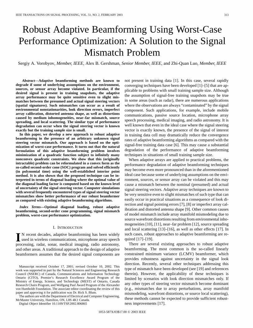
Fig. 1. Output SINR versus training sample sizeN ; first example.

IV. SIMULATIONS

In our simulations, we assume a uniform linear array withomnidirectional sensors spaced half a wavelength

apart. For each scenario, 200 simulation runs are used to ob-tain each simulated point. In all examples, we assume two in-terfering sources with plane wavefronts and the directions ofarrival (DOAs) 30 and 50 , respectively. In all simulations, theinterference-to-noise ratio (INR) in a single sensor is equal to30 dB, and the signal is always present in the training data cell.Four methods are compared in terms of the mean output SINR:the proposed robust beamformer (38), the SMI beamformer (8),the LSMI beamformer (14) withad hocchoice of the diagonalload,8 and the eigenspace-based beamformer (17). The optimalSINR (12) is also shown in all figures. The SeDuMi convex op-timization MATLAB toolbox [29] has been used to computethe weight vector of our robust beamformer that employs theconstant throughout the simulations (except one simu-lation in the first example, where is varied; see Fig. 3), as-suming that the nominal steering vector is normalized so that

( 10). The diagonal loading factor istaken in the LSMI beamformer. Furthermore, diagonal loadingwith the same parameter is applied to our robust technique aswell but only in the case when the sample covariance matrix islow rank (i.e., in the case when ).

A. Example 1: Exactly Known Signal Steering Vector

In this example, we simulate a scenario where the actualspatial signature of the signal is known exactly. Note that evenin this ideal case, the presence of the signal of interest in thetraining data cell may substantially reduce the convergencerates of adaptive beamforming algorithms as compared withthe signal-free training data case [6].

In this example, the plane-wave signal is assumed to impingeon the array from . Fig. 1 compares four aforementionedmethods in terms of the mean output array SINR (11) versusthe number of training snapshots for the fixed single-sensor

8This beamformer is hereafter referred to as thead hocLSMI technique.


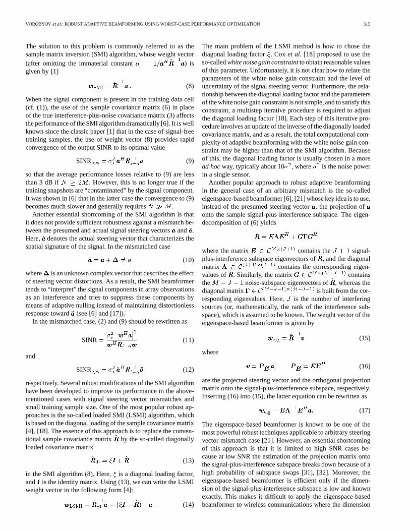
Fig. 2. Output SINR versus SNR; first example.

Fig. 3. Output SINR versus"; first example.

SNR 10 dB. Fig. 2 displays the performance of these tech-niques versus the SNR for the fixed training data size .Fig. 3 shows the performance of the methods tested versusfor

and SNR 10 dB. Additionally, the beampatternsof our beamformer and thead hocLSMI algorithm are com-pared in Fig. 4 for and SNR 10 dB.

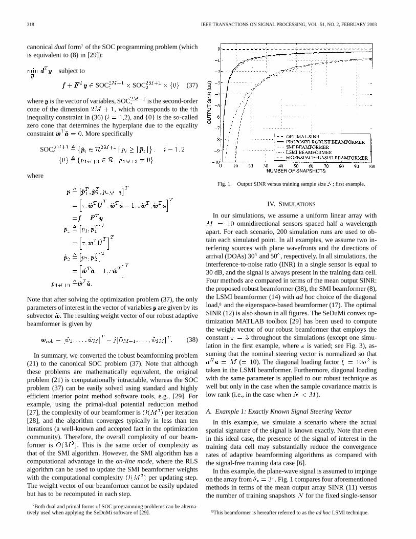
B. Example 2: Signal Look Direction Mismatch

In the second example, a scenario with the signal look direc-tion mismatch is considered. We assume that both the presumedand actual signal spatial signatures are plane waves impingingfrom the DOAs 3 and 5, respectively. This corresponds to a 2mismatch in the signal look direction.

Fig. 5 shows the performance of the methods tested versus thenumber of training snapshots for the fixed SNR 10 dB.The performance of these algorithms versus the SNR for thefixed training data size is shown in Fig. 6.

Fig. 4. Beampatterns of the proposed andad hocLSMI beamformers; firstexample.

Fig. 5. Output SINR versus training sample sizeN ; second example.

Fig. 6. Output SINR versus SNR; second example.


Fig. 7. Output SINR versus training sample sizeN ; third example.

C. Example 3: Signal Spatial Signature Mismatch Due toCoherent Local Scattering

Our third example corresponds to the scenario where the spa-tial signature of the desired signal is distorted by local scatteringeffects. In this example, the presumed signal spatial signature isa plane wave impinging on the array from 3, whereas the actualspatial signature is formed by five signal paths and is given by

(39)

where corresponds to the direct path, whereas ( 1, 2,3, 4) correspond to the coherently scattered paths. We model theth path as a a plane wave impinging on the array from the

direction . The parameters , 1, 2, 3, 4 are independentlydrawn in each simulation run from a uniform random generatorwith mean and standard deviation . The parameters

, 1, 2, 3, 4 represent path phases that are independentlyand uniformly drawn from the interval [0, 2] in each simulationrun. Note that and ( 1, 2, 3, 4) change from run to runwhile remaining frozen from snapshot to snapshot. This casecorresponds to the so-called coherent scattering [14].

Fig. 7 displays the performance of the methods tested versusthe number of training snapshots for the fixed single-sensorSNR 10 dB. Note that the SNR in this example is definedby taking into account all signal paths.

The performance of the same methods versus the SNR for thefixed training data size is displayed in Fig. 8.

D. Example 4: Signal Spatial Signature Mismatch Due toIncoherent Local Scattering

In this example, we assume incoherent local scattering of thedesired signal. The signal is assumed to have a time-varyingspatial signature that is different for each data snapshot and ismodeled as

Fig. 8. Output SINR versus SNR; third example.

where are i.i.d. zero-mean complex Gaussian random vari-ables independently drawn from a random generator. As in theprevious example, the DOAs , 1, 2, 3, 4 are indepen-dently drawn in each simulation run from a uniform randomgenerator with mean and standard deviation . Notethat the DOAs change from run to run while remaining fixedfrom snapshot to snapshot. At the same time, the random vari-ables change both from run to run and from snapshotto snapshot. This corresponds to the case of incoherent localscattering [15], where the signal covariance matrix is nolonger a rank-one matrix, and (11) for the output SINR shouldbe rewritten in a more general form [17]

SINR (40)

The ratio (40) is maximized by [17]

(41)

where is the operator that computes the principal eigen-vector of a matrix. Note that solution (41) is of a little practicaluse because in most applications, the matrixis unknown, andno reasonable estimate of it is available.

Fig. 9 displays the performance of the methods tested versusthe number of training snapshots with the fixed SNR

10 dB. As in the previous example, the SNR is defined bytaking into account all signal paths.

The performance of the same methods versus the SNR forthe fixed training data size is displayed in Fig. 10. Westress that the optimal SINR for Figs. 9 and 10 is computed as

SINR

where is given by (41).

E. Example 5: Near–Far Signal Spatial Signature Mismatch

In the fifth example, we model the so-called near-far spatialsignature mismatch of the desired signal. In this example, the


Fig. 9. Output SINR versus training sample sizeN ; fourth example.

Fig. 10. Output SINR versus SNR; fourth example.

presumed spatial signature of the signal is a plane wave im-pinging on the array from the normal direction 0, whereas theactual spatial signature corresponds to the source located in thenear field of the antenna at a distancefrom the geometrical center of the array, where

is the length of array aperture.9 The source is assumedto be located on the line which is drawn from this geometricalcenter point in the normal direction to the array aperture.

The performance of the methods tested versus the numberof training snapshots for the fixed SNR 10 dB is shownin Fig. 11. Fig. 12 shows the performance of these techniquesversus the SNR for the fixed training data size .

F. Example 6: Signal Spatial Signature Mismatch Due toWavefront Distortion

In our last example, we simulate the situation when the signalspatial signature is distorted by wave propagation effects in aninhomogeneous medium. We assume independent-increment

9Far field condition requires that the distance between the source and antennaremains much larger thanD =� [38].

Fig. 11. Output SINR versus training sample sizeN ; fifth example.

Fig. 12. Output SINR versus SNR; fifth example.

phase distortions of the desired signal wavefront [11], [39]. Ineach simulation run, each of these phase distortions (whichremains fixed for all snapshots) is independently drawn from aGaussian random generator with variance equal to 0.04.

Fig. 13 shows the performance of the methods tested versusfor the fixed SNR 10 dB. The performance of these tech-

niques versus the SNR for the fixed training data sizeis shown in Fig. 14.

G. Discussion

Our simulation figures clearly demonstrate that in all ex-amples, the proposed robust beamformer consistently enjoysthe best performance among the methods tested. Indeed,our new method outperforms the SMI,ad hoc LSMI, andeigenspace-based beamformers, achieving a performance thatis consistently close to the optimal SINR for all values of SNR.Thead hocLSMI algorithm is another well-performing methodas its performance is comparable with that of our robust beam-former in a part of the examples tested. This can be explainedby the fact discovered in Section III that our beamformer ] be-


Fig. 13. Output SINR versus training sample sizeN ; sixth example.

Fig. 14. Output SINR versus SNR; sixth example.

longs to the class of diagonal loading techniques. However, ouralgorithm performs better than thead hocLSMI method in thefourth example at all SNRs (Figs. 9 and 10) and in the second,third, fifth, and sixth examples at high SNRs (Figs. 6, 8, 12 and14). Note that in these examples, the aforementioned perfor-mance gains of our beamformer as compared with thead hocLSMI method can achieve 2 dB. Clearly, this improvement inperformance is due to a more proper choice of the diagonalloading factor in our beamformer as compared with thead hocLSMI beamformer.

The performance of the SMI and eigenspace-based beam-formers is much worse than that of the proposed beamformerand thead hocLSMI beamformer either at high SNRs (as inthe case of SMI beamformer: Figs. 2, 6, 8, 12, and 14) or at lowSNRs (as in the case of eigenspace-based beamformer, the samefigures). Moreover, in the fourth example, the SMI algorithmshows poor performance at all values of the SNR (see Fig. 10).Note that the performance breakdown of the eigenspace-based

beamformer at low SNRs is caused by the subspace swap ef-fect [31], [32], whereas the aforementioned performance lossesof the SMI algorithm at high SNRs are due to the fact that in-creasing the amount of the signal component in the training datais known to lead to a substantial degradation10 of the outputSINR of SMI-type beamformers [6]. Furthermore, from Figs. 1,5, 7, 9, 11, and 13, it follows that the proposed algorithm en-joys much faster convergence rate than the SMI and eigenspace-based algorithms. It is worth noting that even in the situationwithout any steering vector mismatch (Example 1, Figs. 1 and2), the proposed technique has substantially better performanceand faster convergence rate than the SMI and eigenspace-basedbeamformers.

Fig. 3 demonstrates that the proposed beamformer is insensi-tive to the choice of the parameter, whereas Fig. 4 shows thatthe beampatterns of the proposed beamformer and the LSMIbeamformer are very similar to each other. This can be explainedby the above-mentioned fact that the proposed beamformer isequivalent to the LSMI beamformer whose diagonal loadingfactor is optimally matched to the known level of the steeringvector distortion.

V. CONCLUSIONS

A new adaptive beamformer with an improved robustnessagainst an arbitrary unknown signal steering vector mismatchhas been proposed. Our technique optimizes the worst-caseperformance by minimizing the output interference-plus-noisepower while maintaining a distortionless response for theworst-case (mismatched) signal steering vector. A convexformulation for such a robust adaptive beamforming problemis derived using second-order cone programming. It is shownthat the proposed beamformer can be interpreted as a diagonalloading approach whose optimal diagonal loading factor isprecisely computed based on the known level of uncertainty inthe signal steering vector. Computer simulations with severalfrequently encountered types of signal steering vector mis-match show better performance of the proposed beamformer ascompared with several popular robust adaptive beamformingalgorithms.

In addition to the offered performance improvements relativeto existing methods, the proposed beamformer enjoys simpleimplementation. The order of computational complexity ofthis algorithm is comparable with that of the SMI technique.It can be efficiently implemented using currently availableconvex optimization software toolboxes based on interior pointalgorithms.

ACKNOWLEDGMENT

The authors wish to thank the anonymous reviewers fortheir helpful comments and suggestions, which led to theunderstanding of the relationship between our beamformer andthe diagonal loading method.

10This degradation occurs because the signal component “contaminates” thetraining observations (which in the ideal case must contain the interference andnoise components only).


REFERENCES

[1] I. S. Reed, J. D. Mallett, and L. E. Brennan, “Rapid convergence rate inadaptive arrays,”IEEE Trans. Aerosp. Electron. Syst., vol. AES–10, pp.853–863, Nov. 1974.

[2] L. J. Griffiths and C. W. Jim, “An alternative approach to linearly con-strained adaptive beamforming,”IEEE Trans. Antennas Propagat., vol.AP–30, pp. 27–34, Jan. 1982.

[3] E. K. Hung and R. M. Turner, “A fast beamforming algorithm for largearrays,”IEEE Trans. Aerosp. Electron. Syst., vol. AES-19, pp. 598–607,July 1983.

[4] B. D. Carlson, “Covariance matrix estimation errors and diagonalloading in adaptive arrays,”IEEE Trans. Aerosp. Electron. Syst., vol.24, pp. 397–401, July 1988.

[5] R. A. Monzingo and T. W. Miller, Introduction to Adaptive Ar-rays. New York: Wiley, 1980.

[6] D. D. Feldman and L. J. Griffiths, “A projection approach to robustadaptive beamforming,”IEEE Trans. Signal Processing, vol. 42, pp.867–876, Apr. 1994.

[7] L. C. Godara, “The effect of phase-shift errors on the performance ofan antenna-array beamformer,”IEEE J. Ocean. Eng., vol. OE-10, pp.278–284, July 1985.

[8] J. W. Kim and C. K. Un, “An adaptive array robust to beam pointingerror,” IEEE Trans. Signal Processing, vol. 40, pp. 1582–1584, June1992.

[9] N. K. Jablon, “Adaptive beamforming with the generalized sidelobe can-celler in the presence of array imperfections,”IEEE Trans. AntennasPropagat., vol. AP-34, pp. 996–1012, Aug. 1986.

[10] A. B. Gershman, V. I. Turchin, and V. A. Zverev, “Experimental resultsof localization of moving underwater signal by adaptive beamforming,”IEEE Trans. Signal Processing, vol. 43, pp. 2249–2257, Oct. 1995.

[11] J. Ringelstein, A. B. Gershman, and J. F. Böhme, “Direction finding inrandom inhomogeneous media in the presence of multiplicative noise,”IEEE Signal Processing Lett., vol. 7, pp. 269–272, Oct. 2000.

[12] Y. J. Hong, C. C. Yeh, and D. R. Ucci, “The effect of a finite-dis-tance signal source on a far-field steering Applebaum array—Twodimensional array case,”IEEE Trans. Antennas Propagat., vol. 36, pp.468–475, Apr. 1988.

[13] K. I. Pedersen, P. E. Mogensen, and B. H. Fleury, “A stochastic modelof the temporal and azimuthal dispersion seen at the base station in out-door propagation environments,”IEEE Trans. Veh. Technol., vol. 49, pp.437–447, Mar. 2000.

[14] J. Goldberg and H. Messer, “Inherent limitations in the localization ofa coherently scattered source,”IEEE Trans. Signal Processing, vol. 46,pp. 3441–3444, Dec. 1998.

[15] O. Besson and P. Stoica, “Decoupled estimation of DOA and angularspread for a spatially distributed source,”IEEE Trans. Signal Pro-cessing, vol. 48, pp. 1872–1882, July 2000.

[16] D. Astely and B. Ottersten, “The effects of local scattering on directionof arrival estimation with MUSIC,”IEEE Trans. Signal Processing, vol.47, pp. 3220–3234, Dec. 1999.

[17] A. B. Gershman, “Robust adaptive beamforming in sensor arrays,”Int.J. Electron. Commun., vol. 53, pp. 305–314, Dec. 1999.

[18] H. Cox, R. M. Zeskind, and M. H. Owen, “Robust adaptive beam-forming,” IEEE Trans. Acoust., Speech, Signal Processing, vol.ASSP-35, pp. 1365–1376, Oct. 1987.

[19] K. L. Bell, Y. Ephraim, and H. L. Van Trees, “A Bayesian approach torobust adaptive beamforming,”IEEE Trans. Signal Processing, vol. 48,pp. 386–398, Feb. 2000.

[20] M. H. Er and T. Cantoni, “An alternative formulation for an optimumbeamformer with robustness capability,”Proc. Inst. Elect. Eng. Radar,Sonar, Navig., pp. 447–460, Oct. 1985.

[21] L. Chang and C. C. Yeh, “Performance of DMI and eigenspace-basedbeamformers,” IEEE Trans. Antennas Propagat., vol. 40, pp.1336–1347, Nov. 1992.

[22] S. A. Vorobyov, A. B. Gershman, and Z.-Q. Luo, “An application ofsecond-order cone programming to robust adaptive beamforming,” inProc. 5th Int. Conf. Optim. Techn. Applicat., vol. 1, Hong Kong, Dec.2001, pp. 308–315.

[23] , “Robust MVDR beamforming using worst-case performance op-timization,” in Proc. 10th Workshop Adaptive Sensor Array Process..Lexington, MA, Mar. 2002.

[24] , “Robust adaptive beamforming using worst-case performance op-timization via second-order cone programming,” inProc. ICASSP, Or-lando, FL, May 2002, pp. 2901–2904.

[25] M. R. Garey and D. S. Johnson,Computers and Intractability. SanFrancisco, CA: W. H. Freeman, 1979.

[26] R. Lorenz and S. P. Boyd, “Robust minimum variance beamforming,”IEEE Trans. Signal Processing, submitted for publication.

[27] Y. Nesterov and A. Nemirovsky,Interior Point Polynomial Algorithmsin Convex Programming. Philadelphia, PA: SIAM, 1994.

[28] M. Lobo et al., “Applications of second-order cone programming,”Linear Algebra Applicat., pp. 193–228, Nov. 1998.

[29] J. F. Sturm, “Using SeDuMi 1.02, a MATLAB toolbox for optimizationover symmetric cones,”Optim. Meth. Softw., vol. 11–12, pp. 625–653,Aug. 1999.

[30] M. D. Zoltowski, “On the performance of the MVDR beamformer inthe presence of correlated interference,”IEEE Trans. Acoust., Speech,Signal Processing, vol. 36, pp. 945–947, June 1988.

[31] J. K. Thomas, L. L. Scharf, and D. W. Tufts, “The probability of a sub-space swap in the SVD,”IEEE Trans. Signal Processing, vol. 43, pp.730–736, Mar. 1995.

[32] M. Hawkes, A. Nehorai, and P. Stoica, “Performance breakdown of sub-space-based methods: Prediction and cure,” inProc. ICASSP, Salt LakeCity, UT, May 2001, pp. 4005–4008.

[33] S. Cui, Z.-Q. Luo, and Z. Ding, “Robust blind multiuser detectionagainst CDMA signature mismatch,” inProc. ICASSP’01, Salt LakeCity, UT, May 2001, pp. 2297–2300.

[34] Z. Liu and Y. H. Hong, “Semi-infinite quadratic optimization method forthe design of robust adaptive array processors,”Proc. Inst. Elect. Eng.Radar Sonar, Navig., vol. 137, pp. 177–183, June 1990.

[35] M. H. Er and A. Cantoni, “A new approach to the design of broad-band element space antenna array processors,”IEEE J. Ocean. Eng.,vol. OE-10, pp. 231–240, July 1985.

[36] B. D. Van Veen, “Minimum variance beamforming with soft responseconstraints,”IEEE Trans. Signal Processing, vol. 39, pp. 1964–1972,Sept. 1991.

[37] H. Ye and R. D. DeGroat, “A generalized sidelobe canceller with softconstraints,”IEEE Trans. Signal Processing, vol. 40, pp. 2112–2116,Aug. 1992.

[38] P. S. Naidu,Sensor Array Signal Processing. Boca Raton, FL: CRC,2001.

[39] O. Besson, F. Vincent, P. Stoica, and A. B. Gershman, “Maximum like-lihood estimation for array processing in multiplicative noise environ-ments,”IEEE Trans. Signal Processing, vol. 48, pp. 2506–2518, Sept.2000.

Sergiy A. Vorobyov (M’02) was born in Ukraine in1972. He received the M.S. and Ph.D. degrees in sys-tems and control from Kharkiv National University ofRadioelectronics (KNUR), Kharkiv, Ukraine, in 1994and 1997, respectively.

From 1995 to 2000, he was with the Control andSystems Research Laboratory at KNUR, where hebecame a Senior Research Scientist in 1999. From1999 to 2001, he was with the Brain Science Insti-tute, RIKEN, Tokyo, Japan, as a Research Scientist.He is currently with the Department of Electrical and

Computer Engineering, McMaster University, Hamilton, ON, Canada, as a Post-doctoral Fellow. In 1996 and 2002, respectively, he held short-time visiting ap-pointments at the Institute of Applied Computer Science, Karlsruhe, Germany,and Gerhard-Mercator University, Duisburg, Germany. His research interestsinclude control, statistical array signal processing, blind source separation, androbust adaptive beamforming.

Dr. Vorobyov was a recipient of the 1996–1998 Young Scientist Fellowship ofthe Ukrainian Cabinet of Ministers, the 1996 and 1997 Young Scientist ResearchGrants from the George Soros Foundation, and the 1999 DAAD Fellowship(Germany).


Alex B. Gershman (M’97–SM’98) received theDiploma (M.S.) and Ph.D. degrees in radiophysicsfrom the Nizhny Novgorod State University, NizhnyNovgorod, Russia, in 1984 and 1990, respectively.

From 1984 to 1989, he was with the Ra-diotechnical and Radiophysical Institutes, NizhnyNovgorod. From 1989 to 1997, he was with theInstitute of Applied Physics of Russian Academyof Science, Nizhny Novgorod, as a Senior ResearchScientist. From the summer of 1994 until thebeginning of 1995, he was a Visiting Research

Fellow at the Swiss Federal Institute of Technology, Lausanne. From 1995 to1997, he was Alexander von Humboldt Fellow at Ruhr University, Bochum,Germany. From 1997 to 1999, he was a Research Associate at the Departmentof Electrical Engineering, Ruhr University. In 1999, he joined the Departmentof Electrical and Computer Engineering, McMaster University, Hamilton, ON,Canada, as an Associate Professor, where he became a Full Professor in 2002.Currently, he also holds a Visiting Professorship at the Department of Com-munication Systems, Gerhard-Mercator University and Fraunhofer Institutefor Microelectronic Circuits and Systems, Duisburg, Germany. His researchinterests are in the area of signal processing and include robust statistical signaland array processing, adaptive beamforming and smart antennas for mobilecommunications, signal parameter estimation and detection, spectral analysis,and signal processing applications to wireless communications, underwateracoustics, seismology, and radar.

Dr. Gershman was a recipient of the 1993 International Union of RadioScience (URSI) Young Scientist Award, the 1994 Outstanding Young ScientistPresidential Fellowship (Russia), the 1994 Swiss Academy of EngineeringScience and Branco Weiss Fellowships (Switzerland), and the 1995–1996Alexander von Humboldt Fellowship (Germany). He received the 2000Premier’s Research Excellence Award of Ontario and the 2001 Wolfgang PaulAward from the Alexander von Humboldt Foundation, Germany. He is alsoa recipient of the 2002 Young Explorers Prize from the Canadian Institutefor Advanced Research (CIAR), which honors Canada’s top 20 researchersaged 40 or under. Since 1999, he has been an Associate Editor of IEEETRANSACTIONS ON SIGNAL PROCESSINGand a Member of the Sensor Arrayand Multichannel (SAM) Signal Processing Technical Committee of the IEEESignal Processing Society.

Zhi-Quan Luo (M’90) received the B.Sc. degree inapplied mathematics in 1984 from Peking Univer-sity, Beijing, China. Subsequently, he was selectedby a joint committee of American MathematicalSociety and the Society of Industrial and AppliedMathematics to pursue the Ph.D. degree in theUnited States. After a one-year intensive training inmathematics and English at the Nankai Institute ofMathematics, Tianjin, China, he was admitted to theDepartment of Electrical Engineering and ComputerScience, Massachusetts Institute of Technology,

Cambridge, where he received the Ph.D. degree in 1989.Upon graduation, he joined the Department of Electrical and Computer Engi-

neering, McMaster University, Hamilton, ON, Canada, where he is now the De-partment Head and holds a Canada Research Chair in Information Processing.His research interests lie in the union of large-scale optimization, data commu-nication and signal processing, information theory, and coding.

Dr. Luo currently serves on the editorial boards for a number of interna-tional journals including theSIAM Journal on Optimizationand the IEEETRANSACTIONS ONSIGNAL PROCESSING. He is a recipient of the 2001 Awardfor the Best Paper at the International Conference on Optimization Techniquesand Applications.

Robust adaptive beamforming using worst-case …vorobyov/RobBeamformer.pdf · IEEE TRANSACTIONS ON...

Documents

Transcript of Robust adaptive beamforming using worst-case …vorobyov/RobBeamformer.pdf · IEEE TRANSACTIONS ON...