Robotics Research Ibchnical Report

Robotics ResearchIbchnical Report

fi^3

On-line motion planning:

Case of a planar rod

by

James CoxChee-Keng Yap

Technical Report No. 425

Robotics Report No. 187

December, 1988

New York University

Dept. of Computer Science

Courant Institute of Mathematical Sciences

251 Mercer Street

New York, New York 10012

Work on this paper has been supported by Office of Naval Research Grant N00014-85-K-

0046 and bv National Science Foundation Grant No. DCR-84-0189i.

(Technical Report)

On-line motion planning :

Case of a planar rod

James Cox and Chee-Keng Yap

Courant Institute of Mathematical Sciences

New York University

251, Mercer Street

New York, N.Y. 10012

ABSTRACT

In this paper we develop an algorithm for planning the motion of a

planar "rod" or "ladder" amidst an environment containing obstacles

bounded by simple, closed polygons. The exact shape, number and loca-

tion of the obstacles is assumed unknown to the planning algorithm,

which can only obtain information about the obstacles by detecting

points of contact with the obstacles. The abilit>' to detect contact with

obstacles is formalized by move primitives that we call guarded moves.

We call ours the online motion planning problem as opposed to the usual

offline version. This is a significant departure from the usual setting for

motion planning problems, in which the algorithm is given an explicit

description of the scene as part of its input. What we demonstrate is

that the retraction method can be applied, although new issues arise that

have no counterparts in the usual setting. We are able to obtain an algo-

rithm with path complexity {0{k)=0{n-) guarded moves, where n is

the number of obstacle walls, and k the number of pairs of obstacle

walls and corners of distance less than or equal to the length of the

ladder) that matches the known lower bound[Ork85]. This lower bound

holds for both the online and offline (where the environment is expli-

citly given) versions of the problem. The computational complexity of

the algorithm 0{k logn) matches the best known algorithm [Sfs] for the

offline version.

This work is supported by ONR contract N00014-

85-K-0046 and NSF grant DCR-84-0189S.

Section 1. Introduction 2

1. Introdnction

Task planning algorithms and strategies make up an important area of robotics

research. Of great importance is the area of robot motion planning, sometimes also

known as trajectory planning or collision avoidance. Simply stated, the problem is to

navigate a mobile robot or robot arm manipulator through an environment from some

initial position to some target position.

In recent years much work in the area of exact or algorithmic motion planning has

been done. It has been shown that the problem of motion planning is a difficult one

from the point of view of computational complexity, see for

example[Rei79, HSS84, SY84].

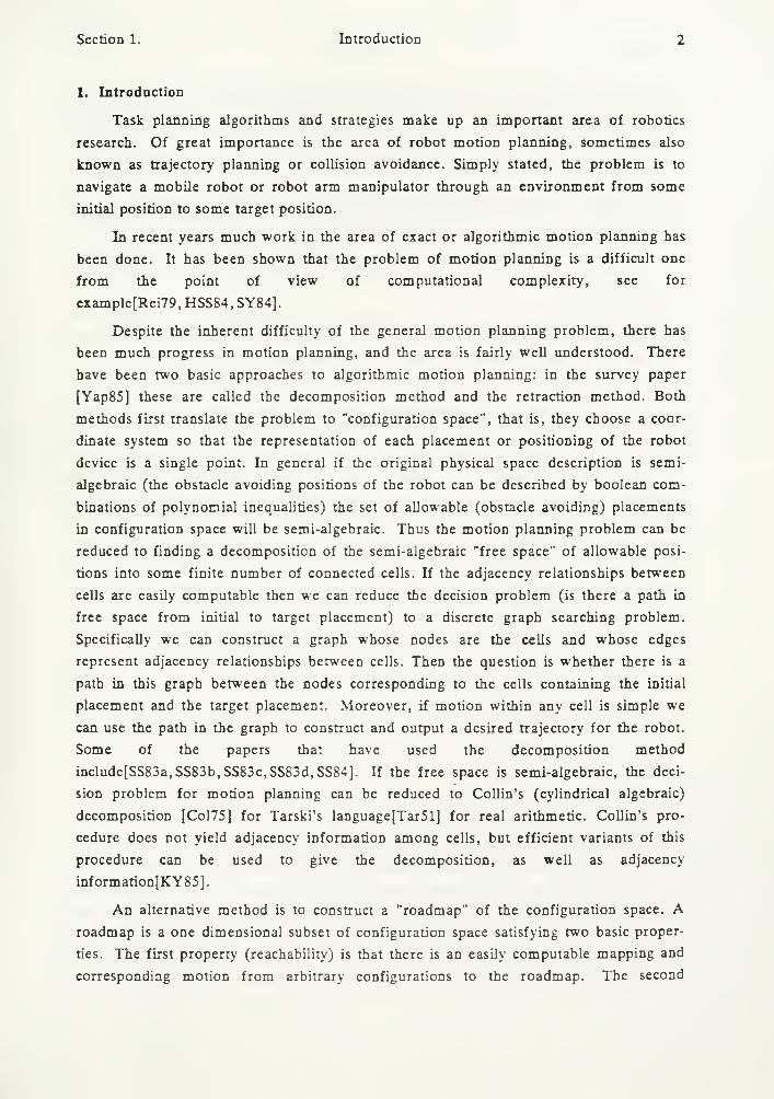
Despite the inherent difficulty of the general motion planning problem, there has

been much progress in motion planning, and the area is fairly weU understood. There

have been two basic approaches to algorithmic motion planning: in the survey paper

[Yap85] these are called the decomposition method and the retraction method. Both

methods first translate the problem to "configuration space", that is, they choose a coor-

dinate system so that the representation of each placement or positioning of the robot

device is a single point. In general if the original physical space description is semi-

algebraic (the obstacle avoiding positions of the robot can be described by boolean com-

binations of polynomial inequalities) the set of allowable (obstacle avoiding) placements

in configuration space will be semi-algebraic. Thus the motion planning problem can be

reduced to finding a decomposition of the semi-algebraic "free space" of allowable posi-

tions into some finite number of connected cells. If the adjacency relationships between

cells are easily computable then we can reduce the decision problem (is there a path in

free space from initial to target placement) to a discrete graph searching problem.

SpecificaUy we can construct a graph whose nodes are the cells and whose edges

represent adjacency relationships between cells. Then the question is whether there is a

path in this graph between the nodes corresponding to the cells containing the initial

placement and the target placement. Moreover, if motion within any cell is simple we

can use the path in the graph to construct and output a desired trajectory for the robot.

Some of the papers that have used the decomposition method

include[SS83a,SS83b,SS83c,SS83d,SS84]. If the free space is semi-algebraic, the deci-

sion problem for motion planning can be reduced to Collin's (cylindrical algebraic)

decomposition [Col75] for Tarski's language[Tar51] for real arithmetic. Collin's pro-

cedure does not yield adjacency information among cells, but efficient variants of this

procedure can be used to give the decomposition, as well as adjacency

information[KY85].

An alternative method is to construct a "roadmap" of the configuration space. Aroadmap is a one dimensional subset of configuration space satisfying two basic proper-

ties. The first property (reachability) is that there is an easily computable mapping and

corresponding motion from arbitrary configurations to the roadmap. The second


property (connectivity) is that the roadmap of a connected component is connected. The

mapping(s) used to construct the roadmap is a retracuon(s), hence the name of the

method. Actually, since in general these mappings will be discontinuous, they will not be

retractions in the proper topological sense of the word but rather "retraction-like".

Retraction has been applied successfully in many problems, see for

cxample[OSY83,OSY86,OSY87,OY85,LS87]; furtiiermore, the method has been shown

to be as general as the decomposition approach[Yap85].

Recently Canny [Can87] gave an algorithm to construct another roadmap of any

semi-algebraic set.

Three recent papers[SH88, Whi85, Yap85] contain good surveys of the area of algo-

rithmic motion planning, as well as a more complete list of references and interesting

variants of the motion planning problem not mentioned here.

Common to the work mentioned above is the assumption that the algorithm is given

an exact representation of the environment as part of its input. Note that the environment

may not be fixed, some obstacles may be moving, e.g.[RS85]. Recently there has been

interest in the problems of robot navigation in the case where little or nothing is known

in advance about the scene. This hearkens back to some of the seminal works in path

planning, such as the maze searching problem[Sut69]. For example, a recent

paper[RSI87] studies the acquisition of knowledge about the environment by a point auto-

maton using some limited computer vision. The authors successfully employ the retrac-

tion approach to this problem setting, in which the environment is planar and contains

polygonal obstacles. We shall call the new class of motion planning problems the online

problems in contrast to the offline problem where the environment is explicitly given.

Lumelsky and Stepanov have studied the online problem of a point automaton mov-

ing in a two dimensional unknown environment consisting of obstacles bounded by simple

closed curves. He assumes only that the automaton can detect contact with obstacles and

that it can follow the border of obstacles. An algorithm which plans the motion of a point

on a two-dimensional surface (and in particular, on a torus) can be translated into an

algorithm for a two link planar robot arm with fully revolute joints and tactile sensing.

Lumelsky has gone on to apply these techniques to several robot arm

arrangements[Lum85a, Lum85b, Lum86, LuS86, Lum87a, Lum87b, LuS87]. However it

had remained unclear whether his technique extends to general robots with more than

two degrees of freedom. This was one of the principle motivations for our work.

In this paper we use a retraction technique to find a nonheuristic algorithm for plan-

ning the motion of the fully three degree of freedom robot "rod" or "ladder" in an

unknown planar environment containing polygonal obstacles. We are able to dynamically

construct a roadmap of the relevant portions of such an environment (those portions that

intersect a given line as in Lumelsky's work) with a motion that has path complexity

bounded by 0{k) = O(n-), where n is the number of obstacle walls and k is the total


number of pairs of obstacle comers and walls within distance less than or equal to the

length of the ladder. This matches the known lower bound[Ork85], and thus the path

complexity of the algorithm is asymptotically optimal. The computational complexity is

0(k logn). and thus matches the complexity of the best known algorithm for the offline

problem[Sfs].

The algorithm solves a type of search by probing problem, related to the recovering

of shape by point and Une probes[Ber86,CY83,DEY86,ES86]. The next section presents

the general framework of our problem.

Section 2. Preliminaries 5

2. Preliminaries

In this paper we consider a mobile robot device B defined by a closed line segment

PQ (see figure 1). Motion planning for the line segment, referred to as the "ladder" or

"rod", moving in the plane or three dimensional Euclidean space amidst known polygonal

or polyhedral barriers has been studied in various papers

[LS85, OSY86, OSY87, Sfs, SS84].

Q

Figure 1 : The ladder or rod with endpoints P and Q

.

We solve our online problem by "retracting" to the topological boimdary of the con-

figuration space. We augment the "natural" vertices and edges of the boundary so that

they form a roadmap of the space.

In this paper B will be free to move in the plane, where we assume a cartesian coor-

dinate frame. The endpoint P is sometimes called the base and Q is called the tip . Both

P and Q will be referred to as ends . Let / be the length of fi = PQ . Sometimes when it

is convenient to think of PQ as a directed segment, we assume a direction from P to Q .

We will illustrate this by putting a dark dot at the base P and an arrow at the tip Q (see

figure 1).

Definition 1. A placement Z for B will mean a triple (x, y , 6), where x and y are the

coordinates of P , and where 6, s 6 < Ztt, is the angle between PQ and the horizontal

ray L extending from P in the positive x direction, measured (clockwise) from L, with

the values and Z-ir identified (see figure 2).

Section 2. Preliminaries

3-17/2

Tt

-n/l

Figure 2 : The angle 6 is measured clockwise from L .

Placements are plainly points in ^-x^', where 3'' is the one dimensional sphere

(circle). The set consisting of aU placements will be denoted by A. We can homeomorph-

ically embed A in if ^ in the following natural way: Let Z = (x,y,e). Then we associate Z

with the point /(Z) = (x cosO, x sinO, y). This mapping / is a continuous one-to-one

embedding (if the space the ladder moves in is restricted to the positive x half-plane) and

allows us to use the Euclidean metric and the standard topology of E^ when we employ

such notions as neighborhoods, continuity, open set, and closed set. We will use Z to

indicate both Z and /(Z) and the distance dist{Z^,Z.^ between two placements is just the

Euclidean distance between f{Z^) and /(Zj). A set of placements will be open if its

image under / is open, etc. If Z is a placement and X is the robot or a subset of the

robot (eg. X - B , P , or Q). Then X[Z] is the set of points in the plane occupied by X

for the given placement. We shall distinguish between the space of placements and the

plane in which the ladder moves by referring to the former as configuration space and the

latter as physical space. Thus a given placement Z in configuration space corresponds to

the set of points B\Z] in physical space occupied by the ladder.

The physical space contains an open set S C J?' with boundary made up of a finite

number of straight line segments. S is called the {polygonal) obstacle set. We assume

R' — S is compact; this can be done by enclosing the scene in a sufficiently large square

(whose sides we regard as fictitious walls). We also assume that the complement of S has

the same interior set as the closure of the complement of S , thus insuring that S contains

no isolated points or "slits". The boundary of 5 is divided into comers and walls (see fig-

ure 3). Corners and walls of S will be referred to as features of 5 , or simply features

.

Section 2. Prelimmaries

a corner

a wall

Fignre 3 : A polygonal obstacle.

We make the following simplifying assumption about the obstacle set: no wall is

parallel to the x-axis of the coordinate frame. This assumption of nondegeneracy simpli-

fies the analysis but is by no means necessary to the construction of the algorithm.

A placement Z is free if B [Z] does not intersect S . The set of all free placements is

denoted by FP . The interior of FP consists of all placements in which the ladder does

not intersect the boundary of S and is plainly a bounded open set. The topological boun-

dary of FP , denoted BFP , is the set of all placements in which B contacts an obstacle

feature (the boundary of 5), that is, either an endpoint of B contacts a wall or B contacts

a comer.

Example 1. Suppose that in position Z, the tip Q of the ladder touches a wall W . Then

we write Q € W or 2 [Z] € W if we want to emphasize the dependence onZ. •

The robot can move in any way it chooses provided the placement remains in FP ,

and, furthermore, for each placement Z in the motion, we assume the robot knows the

setB[Z]n5. Thus the ladder always knows its own position and can detect points where

it contacts the obstacles. We assume that the robot comes equipped with a control system

capable of performing the inverse kinematics enabling either end {P or 2 ) to trace sim-

ple algebraic curves such as a circle or a line. The ladder may be thought of as an auto-

nomous vehicle which can carr>' out "guarded move" instructions consisting of motion

along a smooth curve or a compliant motion which maintains specified obstacle contacts,

until a specific event occurs, such as contact with a new obstacle, or a coordinate taking

on a specified value. These guarded moves are similar to constructs in the high level

real-time programming language COAL introduced by Ernest Davis[Dav84].

Section 2. Preliminaries

The basic problem we solve is the following:

Given Zj € FP , Z^ ^ A, find a path from Zj to Zj if one exists, or else determine

that no path exists.

The algorithm to solve this problem consists of "guarded move" instructions and

regular computer instructions (assignments, loops, test-and-branch, etc.). The guarded

move instructions will be specified by motions which maintain certain constraints.

Example 2. As an example of a guarded move consider the motion given in figure 4. In

this figure the solid ladder represents the initial placement in the guarded move, the

dashed ladder the final placement. The motion maintains two constraints; the wall contact

with the tip and the corner contact with the ladder are maintained throughout the motion.

The motion is terminated by the "event" of the ladder contacting a new obstacle: the base

P contacts a new wall. •

Figure 4 : Example of a guarded move maintaining two obstacle contacts.

We now describe in more detail the types of guarded move instructions .

All guarded move instructions specify 2 "guards" or constraints so that there is a

curve in FP . The instruction will specify which of two directions to move in that curve.

Each constraint is of the form:

1) Maintain contact of the ladder with a particular comer.

2) Maintain contact of a ladder endpoint with a particular wall.

Section 2. Preliminaries 9

3) Maintain a certain orientation of the ladder.

4) Restrict an endpoint of the ladder to move along a particular line in physical space.

We will define the constraints we use for the ladder more formally in the next sec-

tion.

A guarded move is terminated automatically when an "event" occurs.

An event will be one of the following:

a) The ladder msikes a new obstacle contact.

b) One or several of the coordinates reaches some specific value(s).

c) An endpoint (P or Q) reaches some specified point in physical space.

Events may be modeled by some sensor-readouts that can be constantly monitored.

The idea of our algorithm will be to have the ladder search the environment while

keeping in contact with the obstacles, dynamically constructing a roadmap of the environ-

ment as we go. The roadmap will consist of a superset of the edges of the topological

boundary of FP . This roadmap will be an extension and modification of the "extended

vertices graph" of the boundary constructed by Sifrony and Sharir[Sfs], though we only

construct the roadmap on certain "relevant" portions of the boundary. In a sense our

approach will be a synthesis of the retraction technique and the technique of Lumelsky

and Stepanov[LuS86].

Section 3. Constraints 10

3. Constraints

Constraints will be predicates on placements. UK is a constraint listed below the

notation Z\-K (for any placement Z) means Z satisfies the constraint K . The following

constraints will be used:

(1) For each corner C, we say Z I- [B @C] if and only if C € fl [Z]. We shall call these

[B@C] the corner constraints (Figure 5).

(2) For each wall W , and each ladder end E = P ,Q we say Z h [E@W] if and only if

E d W . We call [B@C] the wall constraints (Figure 6).

(3) Z I- [-IT/2], if and only if e[Z] = ts/2. We say B is vertical if 6 = tt/2 (Figure 7).

(4) Z \- [B ±W] if an endpoint of Z contacts W (P or Q d W) and B is perpendicular to

W (Figure 8).

Constraints of type 1 and 2 (comer and wall constraints) will be referred to as obs-

tacle constraints . Constraints of type 3 will be called angle constraints . Constraints of

type 4 will be called perpendicularity constraints .

We will often abbreviate the set of constraints [£@Wj], [ECaW^] for fixed

E = P ,Q by [E@C], where C is the common endpoint of the two walls W^ and Wj.

Also [E@C] implies [B@C] is satisfied.

Figure 5 : A corner constraint [B @C]

Figure 6 : A wall constraint [PCgn']


[^/2]

Figure 7 : An angle constraint [ir/l]

W

Figure 8 : A perpendicularity constraint [B J.W]

The first two types of constraints are natural ways of constraining motion, and the

set of all placements that satisfies one of these obstacle constraints forms the topological

boundary BFP of FP . For each connected component of the topological boundary the

set of placements satisfying two obstacle constraints is not in general a connected set.

The purpose of the perpendicularity constraints is to connect the roadmap on any com-

ponent of the boundary. The angle constraints are used to jump from one component of

the topological boundary to another. The intuition is that we wish to includes motions of

the ladder in our searching that causes the ladder to sweep the maximum possible area

while contacting a given wall, or translating between obstacle clusters, to insure that we

don't "miss anything".


Next we examine dependency among constraints.

Definition 2. Three different constraints K ^, K^, and ^3 are dependent if they have one

of the following 4 forms :

(1) Three corners on B are dependent, that is, for comers of S Cj, (J= 1, 2, 3),

Kj = [A,(aC,] (Figure 9).

(2) Any three constraints consisting of two comer constraints and a wall constraint, in

which the wall W and both comers are colinear are dependent. So for comers C,,

C2, and wall TV of 5 and E = P or Q , the three constraints [B@C,], [fiCgCj], and

[£(2)^] are dependent if W , C,, and Cj lie on the S2ime line (Figure 10).

(3) Any three constraints consisting of an angle constraint and two corner constraints

are dependent, that is for z = 0, tt/2, -rr, or 3-71/2 and comers Cj and C2, the con-

straints [B@Ci], [B@C2], and [z] are dependent (Figure 11).

(4) If the three constraints represent a comer C contacting an endpoint of the ladder we

take the three constraints to be independent unless the ladder is aligned with one of

the walls W which intersect at C ; that is, B and W are colinear.

If three constraints are not dependent they are said to be independent

.

Figure 9 : Three corner constraints still leave B free to

slide in a straight line.


Figure 10 : Three dependent constraints maintained by

a motion in which B slides against the wall.

Figure 11 : B can slide vertically while maintaining the

two corner contacts.


the curve is

2 -yl d^x^ = 3,2 — 1

The following two lemmas indicate that each independent constraint removes a

degree of freedom.

Lemma 1. For any two independent constraints K ^ and Kj, the set of placements in FP

that simultaneously satisfy Jf , and ^j " ^ (possibly empty) one dimensional set.

Proof. This is clearly true in general for two obstacle contacts (constraints), see for

example[Sfs]. In case one of the constraints is an angle constraint, an additional obstacle

contact restricts motion to a one dimensional set. That is, the ladder can only translate

while moving P along a line parallel to W in the case of a wall constraint, or translate

along the line through B in the case of a corner constraint. Finally the placements satis-

fying a perpendicularity constraint are already a one dimensional set, as B can only

translate while maintaining the perpendicular contact with the associated wall. Q.E.D.

Lemma 2. The set of placements in FP simultaneously satisfying any three given in-

dependent constraints is a finite set.

Proof. From the above proof we can show that any pair of these constraints restricts

one endpoint of the ladder to move along a planeir curve, with at most two placements

satisfying the pair for each such endpoint position on the curve. Thus there are 3 planar

curves determined by 3 independent constraints. One can then show that these curves do

not overlap: any two of them intersect a finite number of times. The endpoint is res-

tricted to the finite set of points (at most eight) determined by the intersection points of

any two of these planar curves (which will each be a line segment, a circle, or a con-

choid), with at most two placements for each such point. Q.E.D.

Section 4. The Roadmap of FP 15

4. The Roadmap of FP

The set of placements satisfying two independent constraints is a one dimensional

complex which may be viewed as a network. In this section we show that this network

forms a "natural" roadmap that can be used to solve a certadn normalized motion plan-

ning problem. We show that given the starting and target placements of such a problem

we can appropriately augment the natural roadmap (along a single line in configuration

space) so that it is "connected enough" to solve the normalized problem. In section 5 we

use this solution to solve the general online motion planning problem for the ladder.

Accordingly we make the following definition.

Definition 3. Let D be a component of FP and p = BFP (ID be the topological boun-

dary of D . We define the "natural" network G^ C ^ with respect to D as follows: the

vertices V (called natural nodes) will consist of a vertex Z for each placement Z d D that

satisfies 3 independent constraints. The edge set E (called natural arcs) will consist of

an edge for each closed curve segment of placements 7 C D that satisfies the following

three properties:

(i) Each placement in y satisfies two independent constraints.

(ii) The endpoint placements of -y are natural nodes of G,^,.

(iii) No natural node is in the interior of 7.

We can label the edges or natural arcs of Gj^ by the pair of nodes it connects,

together with two independent constraints satisfied by the placements on the correspond-

ing curve -y.

Let D be a component oi FP . D is connected and compact. The topological boun-

dary 3 = BFP no oi D consists of a finite number of components 3,, i = 0, . . . , m .

These components roughly correspond to clusters of obstacles (see figure 13).


Figure 13 : Three different components of the boundary. Each

component consists of all placements in which the ladder contacts

one of the three obstacles shown.

Lemma 3. The portion of the roadmap in a component p, of the boundary of D is con-

nected, that is Gjjn n p, is connected.

Proof. In [Sfs] it is shown that the set of placements which satisfy two independent

obstacle and/or perpendicularity constraints on a component 3, of the boundary is a con-

nected set. The set of placements which simultaneously maintain an obstacle and an

angle constraint form arcs whose endpoints are placements satisfying two obstacle and/or

perpendicularity constraints, £md thus the addition of these arcs does not change the con-

nectivity of the roadmap on P,. Q.E.D.

In developing our algorithm we will exploit several topological properties of sets in

Let D be the closure of a bounded connected open set in in i?-', so that D is compact

and connected. Let 3 denote the topological boundary of D , and suppose that P consists

of a finite number of components, so that 3 = UPi- ^^^ ^' denote the complement of

1 = 1


D . Then B and D have the following topological properties.

Lemma 4. There exists a unique boundary component (which we take to be ^q) which

separates the interior ofD from points at infinity.

Proof. See the proof of lemma 3.1 in [Sfs]. Q.E.D.

Lemma 5. Let H be an open connected component of D'^ . Then the boundary of H is

entirely contained in a single component $, o/p.

Proof. See lemma 3.2 of[Sfs]. Q.E.D.

Definition 4. Let Zj be the initial placement and Zj the final or target placement. If both

Zj and Z; satisfy [tt/2] (the ladder is vertical in both placements), then this is called a

normalized motion planning problem.

Recall our homeomorphic embedding of A in R^ given by

/(Z) = (a:[Z]cose[Z], x[Z]sine[Z], y[Z]) where we assume that x[Z]>0 (see section 2).

Observe that if e[Z] = it/2, f(Z)=(0,x[Z],y[Z]). Thus there is a one-to-one

correspondence between the positions P[Z] of the base of the ladder in physical space for

placements Z in which the ladder is vertical and points in the y ,z plane in R^ (configura-

tion space embedded in R^). In what follows when we refer to configuration space we

refer to this embedding in R^.

Let us suppose we Jire given a particular instance of a normalized motion planning

problem, with the initial placement Z, € D a component of FP . Let 7 be the straight

line in configuration space connecting /(Z,) and/(Z;). Consider y O D . It will consist of

a finite number of closed line segments (and/or points) 7, » = 1, . . . , n , the endpoints

of which are placements on the topological boundary of D , p (see figure 14).


Figure 14 : The line 7 as it enters and leaves components of

D'^. The dotted lines are in D'^ and the dark cnrves

indicate portions of the boundary of D that interesect the y ,z plane.

Let Gjjj, be the natural network defined on D . We define the extended network as

follows:

Definition 5. Let G'^^ be the union of G^^ with y tl D , where each 7, is called a jump or

pseudo arc of G^ .

Lemma 6. Each placement in a jump 7, satisfies [tr/l]

Proof. From our previous observation both/(Zi) and/(Z2) lie in the y ,z plane of

configuration space. Thus the line 7 connecting these points in R^ will also lie in this

plane and each placement will clearly satisfy [tt/Z].

Lemma 7. There is a path in FP from Z, to Zj if and only if there is a path from Zj to

Z.inGl^.

Proof. If no path in FP exists then clearly no path in G*„ exists, as Gj^, C FP

.

Suppose that there is a path in FP from Zj to Z^, thus both initial and target placements

are in D . Consider two adjacent jump segments 7, and 7,*], so that one endpoint place-

ment Z of 7, and one endpoint placement Z' of 7, + jare connected by an open segment

a C 7 lying entirely in D' . Now a hes in the same component H of D*^, and thus by

lemma 5 both boundary point placements Z and Z' lie on the same component p, of the

boundary of D . Further since both Z and Z ' satisfy [tt/Z] as well as an obstacle constraint


(they are in BFP) they both lie on the roadmap G[n, n p,. Thus by lemma 3 there is a

path 17, in Gjn, from Z to Z' (note that this path may leave the y ,z plane). It follows that

the path composed of the concatenation of all the -y, and it,, 7i;'iTi;"y2; * " ' ;if„;*y„, is the

desired path in Gj„, from Zj to Zj. Q.E.D.

Section 5. Solving the Online Motion Planning Problem 20

5. Solving the Online Motion Planning Problem

In this section we show how to use the solution of the normalized problem to solve

the general problem for moving the ladder. First we show the reachability of the road-

map Gj„ from any initial placement. Suppose we are given a target placement Z2. We can

always rotate the coordinate frame of physical space so that we may assume without loss

of generality that Z^^l-n/l].

Definition 6. For any initial placement Zj, Im(Z,) is the placement obtained by the fol-

lowing procedure:

1) We rotate the ladder B in a clockwise direction about PfZj] until either B becomes

vertical or is blocked from further rotation by an obstacle. Let Z be the result of

this motion.

2) If Z satisfies two independent constraints then Im(Zi) = Z. Otherwise we have two

cases.

Case 1

If Z is vertical translate B toward the target until either we reach the target, or B is

blocked by an obstacle. That is, Im(Zj) is the final placement in the motion which

translates B from its position in Z by moving P along the line segment in physical

space between P[Z'] jmd /'[Z^] until B either reaches Z^ or is blocked by an obsta-

cle.

Case 2

Else Z satisfies an obstacle constraint K . We rotate fl in a clockwise manner about

the point of contact with the feature until we reach a placement Z ' which satisfies

two constraints. We set Im(Zi) = Z'.

Example 3. In figure 15 we see an example of the action of Im. The solid ladder is Z, the

dashed ladder the result of step 1 of the above procedure, and the dotted ladder is Im(Z).


Figure 15 : Example of the motion from Z to Im(Z).

Lemma 8. Either Im(Z,) € G^^ or Im(Z,) = Zj.

Proof. By construction of Im either we reach Z, or Im(Zi) satisfies two independent

constraints. Q.E.D.

We now show that if Z^ is reachable then each component of Gj^, has a placement in

which the rod is vertical.

Definition 7. A convex corner C is vertically free if it has the highest y coordinate

among all obstacles in a sufficiently small neighborhood of C . We call a placement Z

vertically free if ZI-[ii/2] (is straight) £ind the endpoint Q contacts a vertically free con-

vex comer C of 5 so that the incident walls of C lie below the horizontal line through

P [Z] and B is free to translate along its length from upwards from Z.

Example 4. In figure 16 we see an example of a vertically free placement of the ladder.


Figure 16 : Vertically free placement of the ladder

Lemma 9. Let p^ be a component of the boundary of D . If there is a path from Zj to

Zj in D then there is a placement Z € 3, which satisfies [17/2]. Further Z € Gj^,

Proof. If 3, is the entire boundary of D then clearly there must be a placement

which satisfies [-n/l] since we can always translate B from its position Ln Zj to a place-

ment in which B contacts an obstacle.

So suppose p, is not the only component of the boundary. According to lemma 4

there is a unique external boundary component; all other components are internal boun-

dary components. In case p, is an internal boundary component, then choose a placement

on P, of maximal z coordinate (recall that under our embedding /, this placement max-

imizes the y coordinate of P among all placements in p,). A straightforward, though

somewhat detailed argument (see lemma 3.5 in[Sfs] for details) shows that at least one

such placement Z will be a vertically free placement, which clearly satisfies three

independent constraints.

Similarly, if p, is the external boundary component then choose among all internal

boundary components the highest vertically free placement Z. By translating B vertically

from Z until it contacts the external boundary, we obtain a placement on p, in which the

ladder is vertical, and thus satisfies at least two constraints. Q.E.D.

We now use the solution to the normalized problem to solve our general problem.

By the previous lemma we may choose a placement Z on the same component of the


roadmap G^^ as Im(Zi) so that Z\-[-n/2]. We now have a normalized problem to solve.

Theorem 10. Let Z be a vertical placement on the same component of Gi^ as Im(Z^).

Let G^ be the extended network with respect to the line y connecting Z and Zj. Then

there is a path from Z j fo Zj if and only if there is a path in G^ from Im(Zi) to Zj.

Proof. For the nontrivial direction of the proof assume that there is a path in

D C FP ,(the component containing Z,) from Z, to Z,. Then by lemma 9 the placement

Z\-[-n/2\ on the same portion of the roadmap as Im(Zi) exists. Since by assumption both

Z and Z2 are in D then from lemma 7 there is a path from Z to Z^ in Gi'^, . By lemma 3

there is a path from Im(Z]) to Z , and concatenating this with the path from Z to Zj gives

the desired final path. Q.E.D.

Section 6. The Searching Algorithm and Computation 24

6. The Searching Algorithm and Computation

In this section we show how to carry out the search for a given instance of the prob-

lem. This amounts to showing how to implement a depth first search of the roadmap and

the jumps using guarded moves and ordinary computer instructions. From our initial

placement Zj we we move to a natural arc of the network by the motion from Zj to

Im(Z,). This can clearly be carried out with two guarded moves. We then search along

the Gj^ roadmap for a placement Z satisfying [tt/I]. We now record the line segment T

in physical space which connects P[Z] and /'[Zj. This line segment in physical space

corresponds to a line segment 7 in configuration space. We will augment the natural

roadmap by jumps which amount to translations along this line. Eventually we either

reach our target Z2, or else if we have explored the entire roadmap Gj^ on the com-

ponents of the boundary which intersect 7 and Zj is not reachable we can stop, assured

that no path to the target exists.

There are several issues that must be dealt with in order to carry out the search out-

lined above. First we must show how to search along the natural arcs of Gjj,,. This

amounts to showing how to reduce the appropriate constrained motions to guarded

motions and how to detect, name and keep track of constraints. We also need a way of

detecting nodes that have been previously visited. Then we must show how to find and

follow jumps.

Under our model we assume we can detect contact points of obstacles with the

ladder B , as well as their location in physical space. We can assign names to our walls

and corners in a straightforward manner. Walls can be named by the equation of the line

through them. The coordinates in physical space of a comer can be used to name the

comer. We assume as part of our model that the ladder endpoints P and Q come

equipped with tiny sensing devices that enable us to determine the direction of a wall we

contact and thus allow us to determine when we contact an obstacle corner. We can then

detect when P or Q contacts a corner and the directions of the incident edges. Thus the

maintaining constraints can be accomplished by inverse kinematics, which is equivalent in

this setting to having the ability to perform compliant motions. For maintaining two con-

straints where one is an an angle or perpendicularity constraint, we see that in each case

the motion involves translating B so that an endpoint of B moves along a specific line in

physical space. Similarly two obstacle constraints involve moving endpoints along lines

and/or conchoids.

We can name nodes by the coordinates of the placement itself. In order to perform

a depth first search from a given node we need a data structure that will allow us to

determine if a node has been previously visited.

For this purpose we use a balanced binary search tree, ordered lexicographically on

the three coordinates. We prefer the the self-adjusting splay trees of Tarjan and

Sleightor[Tar83]. Using this data structure T, and a stack S we now show how to


construct and search the network which comprises G'„ .

Main Algorithm

Inpnt:

Initial placement Zj and target placement Zj

Oatput:

A graph G consisting of all placements in Gj^, (with respect to a specific line seg-

ment 7), reachable from Zj, including a path from Zj to Zj if one exists.

Initialization:

1) Initially record "y as "unspecified". We move from Z, to Im(Z,).

2) Im(Z]) now satisfies 2 independent constraints K^ and ^j. We follow these to a

node V. We insert this node into a splay tree T. For each pair of independent con-

straints K, ,Kj that V satisfies and each direction s = ± , we push the tuple

(v ,X, ,Kj s ) onto a stack S .

Search Loop:

While the stack S is not empty we repeat steps 3 and 4.

3) Pop the top of S .

Case 1:

If this tuple contains the current node v (corresponding to the current placement of

the ladder) we follow the arc a specified by the constraints and sign, if this motion

is possible. If we reach Z; we go to step 5. Otherwise the guarded move will ter-

minate in a node u. Note that this arc a may specify a jump (see step 4). Wecheck if the node u reached is present in T, and if not we insert it into T and pop

the appropriate tuples (u ,K^,Kj,s) onto the stack, with the exception of the tuple

that specifies the arc a that we have just traversed. Else if u is previously visited,

we backtrack to v, by inverting the guarded move a.

Case 2:

If the popped tuple specifies a node v which is not the current node, we backtrack

to node v by inverting the guarded move given by the tuple.

4) If -y has been specified and any placement Z on a intersects -y, and Z is not in T , we

insert Z as a (pseudo-) node in T , and pop the appropriate tuple (which specifies a

the guarded move along -y toward Zj) onto the stack 5. Else if 7 has not yet been

specified and any placement on a satisfies [11/2], we specify y as the line segment

that connects Z with Z,, where Z is the first such placement encountered on a.


5) If we have reached Zt we are done. Otherwise the stack is empty and we have

searched all of Gj'^, and have not reached our target, so we terminate the search in

failure.

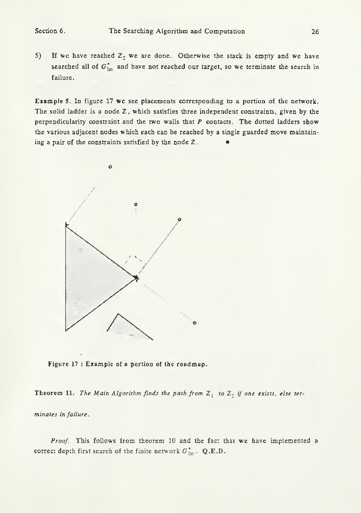
Example 5. In figure 17 we see placements corresponding to a portion of the network.

The solid ladder is a node Z, which satisfies three independent constraints, given by the

perpendiculmty constraint and the two walls that P contacts. The dotted ladders show

the various adjacent nodes which each can be reached by a single guarded move maintain-

ing a pair of the constraints satisfied by the node Z. •

Figure 17 : Example of a portion of the roadmap.

Theorem 11. The Main Algorithm finds the path from Z, to Z-, if one exists, else ter-

minates in failure.

Proof. This follows from theorem 10 and the fact that we have implemented a

correct depth first search of the finite network Gj'^. . Q.E.D.


Note that as a heuristic alternative we could, for each component of Gj^,, take only

the jump from the intersection point with -y which is closest to Z^. Also we could give

preference to arcs maintaining [tt/Z] in the hope that we can go around the "virtual" con-

figuration space obstacle represented by a component of the topological boundary while

keeping the ladder vertical. Of course in general this will not be true, and we will have to

leave the y ,z plane in configuration space in order to reach the arc of Gj^ which next

interseas -y.

Section 7. Complexity of the Searching 28

7. Complexity of the Searching

We now bound the size of the network built by the search procedure.

Theorem 12. The size of the network G^ is O(n^).

Proof. The set of natural arcs which satisfy two independent obstacle and/or per-

pendicularity constraints has complexity O(n^), see for example [Sfs]. An arc a which

maintains an angle constraint intersects at most two of the above arcs (at the endpoints of

a). Since each of the above boundary edges can contain at most 1 placement which satis-

fies an angle constraint, these constraints add at most O(n^) nodes and arcs to the natural

network. It follows that the total complexity of the natural network is bounded by

Similarly the jumps maintain an angle constraint and thus induce at most one new

node per natural arc. Actually since each jump encounters a new obstacle feature, it is

easy to show that there are at most 0{n) jumps. Q.E.D.

Theorem 13. The searching of the network FPj takes 0(n^) guarded move instructions.

Proof. Since following an arc or a jump takes one guarded move, the entire depth

first search takes O(n^) guarded moves. Q.E.D.

Now the computational complexity of our algorithm is proportional to the number

of guarded move instructions executed. In particular since we use splay trees (any bal-

anced tree scheme will do) to store nodes (for checking if a a node has been previously

visited) the total complexity of the finds and inserts is at most 0(n*logn). This is

asymptotically as efficient as the previous best algorithms in the case of a known environ-

ment, and the O(n') path complexity of G[^ matches the known lower bound.

Also in the case of an obstacle set with a fairly large clearance between obstacles

(greater that /) the algorithm will be much more efficient. In particular if ifc is the

number of pairs of features that the ladder can simultaneously contact while remaining in

FP then the complexity is 0{klogn), as in [Sfs]. Further since we only search com-

ponents of the boundary which intersect the line 7, the actual searching may be much

more efficient, as we will not explore obstacle clusters which do not interact with those

on this line.

Section 8. Conclusion 29

8. Conclusions and Future Directions We have demonstrated that a fully three degree

of freedom robot device can search an unknown environment using idealized tactile sens-

ing. The algorithm is exact and non-heuristic in nature, and its worst case path complex-

ity is asymptotic2dly optimal. This suggests other natural problems.

First of all there is the generalization of the probing problem. How can various

manipulators and robots learn about an environment by tactile probes? As mentioned

before, probing problems have been studied, for example in[CY83]. How does an arbi-

trary manipulator probe an environment and determine the shape of objects in the scene?

In the doctoral dissertation of the first author[Cox88] we solve the same problem

for a three link robot arm. In this case the connectivity of the roadmap is much harder to

show. In particular rather than an explicit analysis of the connectivity of the topological

boundary, an analysis of the discontinuities of the retraction used is required to insure

connectivity of the roadmap. Thus there are more "jumps" required, and further secon-

dary (perpendicularity) constraints are introduced. The analysis is more difficult because

of the complex way in which a linkage with rotational degrees of freedom can move, and

the resulting geometry is more intricate. In the case of the arm it might be that the set of

placements satisfying two primary constraints (obstacle and angle constraints) is already

connected. Can one show that this set of naturally constrained motions forms a con-

nected "roadmap" of each component of FP ? What is the performance of the heuristic of

searching the natural network first, with preference given to pairs of primary constraints?

For a linkage can we search only the roadmap of components which intersect a given line,

such as the Af -line in some of Lumelsky's algorithms[Lum85a,Lum85b] as we have done

with the ladder? Also what is the performance of the heuristics for the ladder suggested

at the end of section 6 of this paper?

One can generalize this approach to manipulators and general robots with more (A)

degrees of freedom and to navigating in a "work space" of three dimensions. In the case

of a linkage it seems that a separate analysis is required for each k . Is there a general

approach to choosing a retraction that works for arbitrary robot bodies and degrees of

freedom? Also for k degrees of freedom general considerations reyeal that the set of con-

strained motions will be a set of size 0(n*). Can we get a better bound than this?

Perhaps we can use one retraction to prove connectivity, another to show reachability.

Since constrained motions search the topological boundary of FP , an analysis of connec-

tivity can be independent of the reachability analysis, as demonstrated in [Sfs] and in this

paper.

Since the discontinuities of a retraction are considerably simpler for translational

motions perhaps a general method for robot systems with at most one rotational degree

of freedom may be obtained. The first author is currendy developing an algorithm for

moving any convex polygon in an initially unknown polygonal environment.

Section 8. Conclusion 30

Finally these type of problems lead to different formulations of the notion of com-

putational complexity and new issues in algorithm design. [Lum87b] contains an interest-

ing discussion of these novel issues.

References 31

REFERENCES

[Ber86]. Herbert Bernstein, "Determining the shape of a convex n -sided polygon by

using 2n^k tactile probes," Information Processing Letters 22 pp. 255-260

(1986).

[Bol64]. Vladmir Boltianskii, Envelopes, Macmillan (1964).

[Can87]. J. F. Canny, "A new algebraic method for motion planning amd real

geometry," 28th FOCS, pp. 39-48 (1987).

[CY83]. R. Cole and C. Yap, "Shape from probing," /. Algorithms) 8 pp. 19-38

(1987).

[Col75]. G. E. Collins, "Quantifier elimination for real closed fields by cylindrical

algebraic decomposition," 2nd GI Conference on Automata Theory and Formal

Languages 33 pp. 134-183 Springer-Verlag, (1975).

[Cox88]. J. Cox, "Online motion planning," PhD. Thesis, (1988). New York Univer-

sity

[Dav84]. Ernest Davis, "A high-level real time programming language," Robotics

Rept. 36, New York University (Oct. 1984).

[DEY86]. D. Dobkin, Herbert Edelsbrunner, and Chee K. Yap, "Probing convex

polytopes," I8th STOC, pp. 424-432 (1986).

[ES86]. Herbert Edelsbrunner and Steven S. Skiena, "Probing convex polygons with

X-rays," Univ. of Bl. at Urbana-Champaign, Computer Science Dept., Rep.

No. UIUCDCS-R-86-1306 (November 1986).

[HSS84]. J. E. Hopcroft, J. T. Schwartz, and M. Sharir, "On the complexity of motion

planning for multiple independent objects; PSPACE hardness of the

"warehouseman's problem"," NYU-Courant Institute, Robotics Lab. Report

No. 14 (Feb. 1984).

[KY85]. D. Kozen and C. Yap, "Algebraic cell decomposition in NC," Proc. IEEESymp. Found. Comput. Sci. 26 pp. 515-521 (1985).

[LS85]. D. Leven and M. Sharir, "An efficient and simple motion planning algorithm

for a ladder moving in two-dimensional space amidst polygonal barriers,"

Computational Geometry 1 pp. 221-227 (1985).

[LS87]. D. Leven and M. Sharir, "Planning a purely translational motion for a convex

object in two-dimensional space using generalized Voronoi diagrams,"

Discrete and Computational Geometry 2 pp. 9-31 (1987).

[Lum85a]. V. J. Lumelsky, "On dynamic path planning for a planar robot arm,"E.E.TR-8505, Yale University (AprU 1985).

[Lum85b].

V. J. Lumelsky, "Continuous path planning for various planar robot arm con-

figurations," E.E.TR-8506, Yale University (May 1985).

[LuS86]. V. J. Lumelsky and A. A. Stepanov, "Dynamic path planning for a mobile

automation with limited information on the environment," IEEE Trans.

Automatic Control AC-31(11) pp. 1058-1063 (Nov 1986).

[Lum86]. V. J. Lumelsky, "Continuous motion planning in an unknown environment

for a 3D Cartesian robot arm," Proceedings 1986 IEEE Conference on Robotics

and Automation 2 pp. 1050-1055 (April 1986).

References 32

[LuS87]. V. J. Lumelsky and A. A. Stepanov, "Path-planning strategies for a point

mobile automaton moving amidst unknown obstacles of arbitrary shape.,"

Algorithmica, (2) pp. 403-430 (1987).

[Lum87a]. V. J. Lumelsky, "Dynamic path planning for a planar articulated robot armmoving amidst unknown obstacles," Automatica 23(5) pp. 551-570 (June

1987).

[Lum87b].

V. J. Lumelsky, "Algorithmic and complexity issues of robot motion in an

uncertain environment," Journal of Complexity 3(2) pp. 146-182 (1987).

[OSY83]. C. 6'Dunlaing, M. Sharir, and C. K. Yap, "Retraction: A new approach to

motion planning," 15th FOCS, pp. 207-220 (1983). (also, chapter 7 in Plan-

ning, Geometry, and Complexity, eds. Hopcroft, Schwartz and Sharir, AblexPub. Corp., Norwood, NJ 1987)

[OY85]. C. O'Diinlaing and C. K. Yap, "A retraction method for pl£inning the motion

of a disc," J. Algorithms 6 pp. 104-111 (1985). (also, chapter 6 in Planning,

Geometry, and Complexity, eds. Hopcroft, Schwartz and Sharir, Ablex Pub.

Corp., Norwood, NJ 1987)

[OSY86]. C. O'Diinlaing, M. Sharir, and C. K. Yap, "Generalized Voronoi diagrams

for moving a ladder: L topological analysis," Comm. Pure and AppL Math.

XXXEX pp. 423-483 (1986).

[OSY87]. C. O'Diinlaing, M. Sharir, and C. K. Yap, "Generalized Voronoi diagrams

for moving a ladder: 11. Efficient construction of the diagram," Algorithmica

2 pp. 27-59 (1987).

[Ork85]. J. O'Rourke, "A lower bound for moving ladder," Tech. Rept. JHU/EECS-85/20, Johns Hopkins University (1985).

[Pau81]. R. P. Paul, Robot Manipulators: Mathematics, Programming and Control, MITPress (1981).

[RSI87]. N. S. V. Rao, N. Stoltzfus, and S. S. Iyengar, "The terrain acquisition by

mobile robots. FV. A retraction method," C.S.TR-87-013, Louisiana State

University (1987).

[RS85]. J. Reif and M. Sharir, "Motion planning in the presence of moving obsta-

cles," Proc. IEEE Symp. Found. Comput. Sci. 26 pp. 144-154 (1985).

[Rei79]. John H. Reif, "Complexity of the mover's problem and generalizations,"

20th Proc. IEEE Symp. Found. Comput. Sci., pp. 421-427 (1979). (Also in

Planning, Geometry, and Complexity of Robot Motion, eds. J. Hopcroft, J.

Schwartz, M. Sharir, Ablex Pub. Co., Norwood, NJ, 1985)

[SS83a]. J. T. Schwartz and M. Sharir, "On the piano movers' problem: I. The special

case of a rigid polygonal body moving amidst polygonal barriers," Comm.Pure and Appl. Math. XXXVI pp. 345-398 (1983).

[SSS3b]. J. T. Schwartz and M. Sharir, "On the piano movers' problem: II. General

Techniques for computing topological properties of real dgebraic manifolds,"

Advances in Appl. Math. 4 pp. 298-351 (1983).

[SS83c]. J. T. Schwartz and M. Sharir, "On the piano movers' problem: III. Coordi-

nating the motion of several independent bodies: the special case of circular

bodies moving amidst polygonal barriers," The International J. of Robotics

Research 2(3) pp. 46-75 (1983).

References 33

[SS84]. J. T. Schwartz and M. Sharir, "On the piano movers' problem: V. The case

of a rod moving in three-dimensional space amidst polyhedral obstacles,"

Comm. Pure and Appl. Math. XXXVO pp. 815-848 (1984).

[SS83d]. M. Sharir and E. Ariel-Sheffi, "On the piano movers' problem: IV. Various

decomposable two-dimensional motion planning problems," NYU-Courant

Institute No. 58 (Feb. 1983).

[SS84]. J. T. Schwartz and M. Sharir, "On the piano movers' problem: V. The case

of a rod moving in three-dimensional space amidst polyhedral obstacles,"

Comm. Pure and Appl. Math. XXXVD pp. 815-848 (1984).

[SH88]. M. Sharir, "Algorithmic motion planning," Comp. Sci. TR 392, NYU. (Aug.

1988).

[Sfs]. S. Sifrony and M. Sharir, "An efficient motion planning algorithm for a rod

moving in two-dimensional polygonal space," Algorithmica 2 pp. 367-402

(1987).

[SY84]. P. Spirakis and C. K. Yap, "Strong NP-hardness of moving many discs,"

Information Processing Letters 19 pp. 55-59 (1984).

[Sut69]. I. Sutherland, "A method for solving arbitrary-wall mazes by computer,"

IEEE Trans. Computers C-18(12) pp. 1092-1097 (1969).

[Tar83]. R. E. Tarjan, Data Structures and Network Algorithms, SLAM (1983).

[Tar51]. A. Tarski, "A decision method for elementary algebra and geometry," Univ.

of California Press, (1951). (2nd ed. rev.)

[Whi85]. S. H. Whitesides, "Computational geometry and motion planning," pp.

311-427 in Computational Geometry, ed. G. T. Toussaint,Elsevier Science

Publishers B.V. (North-Holland) (1985).

[Yap85]. Chee K. Yap, "Algorithmic motion planning," in Advances in robotics,

Volume J: algorithmic and geometric aspects, ed. J. T. Schwartz and C. K.

Yap,Lawrence Erlbaum Assoc, Hillsdale, New Jersey (1987).

NYU COMPSCI TR-425Cox, JamesOn-line motion planning:case of a planar rod.

c.l

NYU COMPSCI TR-425- Cox, JamesOn-line motion planning:

- case of a planar rod. -*

c.l 1

Robotics Research Ibchnical Report

Documents

Transcript of Robotics Research Ibchnical Report