Robotics 2014 03 Kinematic functions - … · 2014-03-01 · How to define the robot reference...
64
ROBOTICS ROBOTICS 01PEEQW 01PEEQW 01PEEQW 01PEEQW Basilio Bona Basilio Bona DAUIN DAUIN – Politecnico di Torino Politecnico di Torino
Transcript of Robotics 2014 03 Kinematic functions - … · 2014-03-01 · How to define the robot reference...

ROBOTICSROBOTICS
01PEEQW01PEEQW01PEEQW01PEEQW
Basilio BonaBasilio Bona
DAUIN DAUIN –– Politecnico di TorinoPolitecnico di Torino

Kinematic functionsKinematic functions

Kinematics and kinematic functions
� Kinematics deals with the study of four functions (called
kinematic functions or KFs) that mathematically transform
joint variables into cartesian variables and vice versa
1. Direct Position KF: from joint space variables to task space
pose
2. Inverse Position KF: from task space pose to joint space 2. Inverse Position KF: from task space pose to joint space
variables
3. Direct Velocity KF: from joint space velocities to task space
velocities
4. Inverse Velocity KF: from task space velocities to joint space
velocities
Basilio Bona 3ROBOTICS 01PEEQW
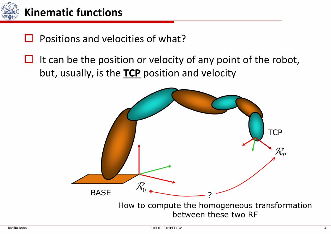
Kinematic functions
� Positions and velocities of what?
� It can be the position or velocity of any point of the robot,
but, usually, is the TCPTCP position and velocity
Basilio Bona 4ROBOTICS 01PEEQW
BASE
TCP
PR
0R?
How to compute the homogeneous transformationbetween these two RF
Kinematic functions
� The first step is to fix a reference frame on each robot arm
� In general, to move from a RF to the following one, it is
necessary to define 6 parameters (three translations of the
RF origin + three angles of the RF rotation)
� A number of conventions were introduced to reduce the
number of parameters and to find a common way to number of parameters and to find a common way to
describe the relative position of reference frames
� Denavit-Hartenberg conventions were introduced in 1955
and are still widely used in industry (with some minor
modifications)
Basilio Bona 5ROBOTICS 01PEEQW

How to define the robot reference frames?
� A RF is positioned on each link/arm, using the so-called
Denavit-Hartenberg (DH) conventions
� The convention defines only 4 parameters between two
successive RF, instead of the usual 6
� 2 parameters are associated to a translation, 2 parameters
are associated to a rotation
� Joints can be prismatic (P) or revolute (R); the convention is � Joints can be prismatic (P) or revolute (R); the convention is
always valid
� Three parameters depend on the robot geometry only, and
therefore are constant in time
� One parameter depends on the relative motion between
two successive links, and therefore is a function of time
� We call this one the i-th joint variable
Basilio Bona 6ROBOTICS 01PEEQW
( )iq t

DH convention – 1
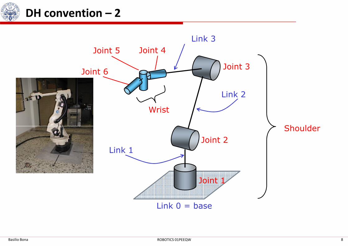
� Assume a connected multibody system with n rigid links
� The links may not be necessarily symmetric
� Each link is connected to two joints, one toward the base, one toward the TCP
We want to locate a RF on this armlink
Basilio Bona 7ROBOTICS 01PEEQW
We want to locate a RF on this arm
toward the base
toward the TCP
link
DH convention – 2
Joint 3
Joint 4
Link 2
Link 3
Joint 5
Joint 6
Wrist
Basilio Bona 8ROBOTICS 01PEEQW
Joint 1
Joint 2
Link 1
Shoulder
Link 0 = base
DH convention – 3
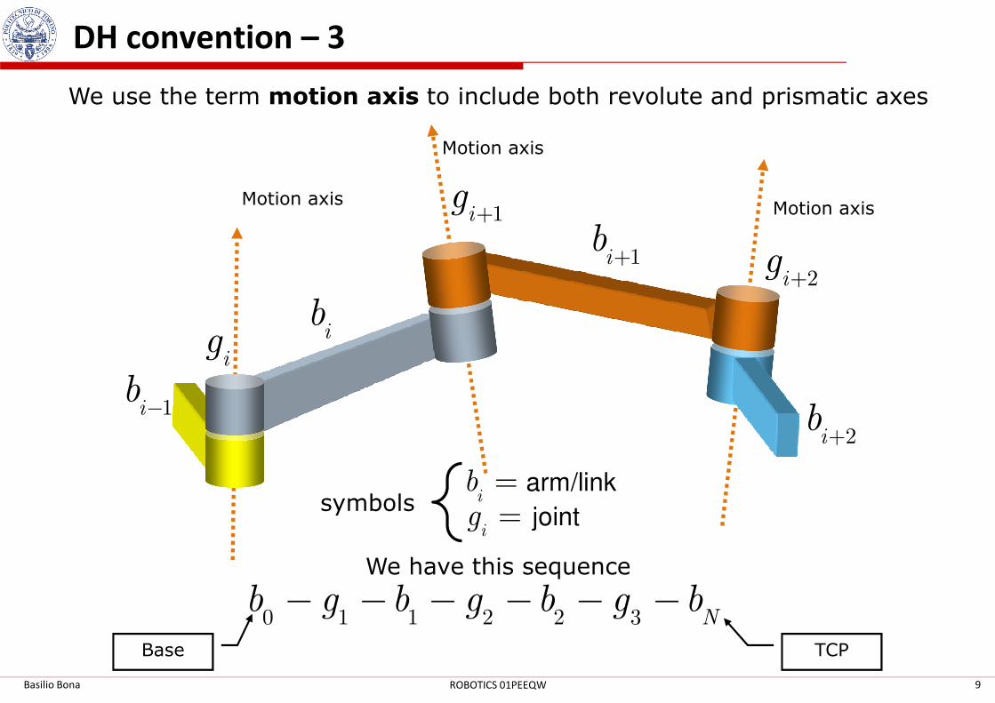
We use the term motion axis to include both revolute and prismatic axes
Motion axis
Motion axis
Motion axis
ig i
b
1ib +
1ig +
2ig +
Basilio Bona 9ROBOTICS 01PEEQW
We have this sequence
0 1 1 2 2 3 Nb g b g b g b− − − − − −
Base TCP
1ib −
ig
2ib +
arm/linkib =
jointig =symbols

DH convention – 4
Basilio Bona 10ROBOTICS 01PEEQW

DH convention – 5
Motion axis
Motion axis
Motion axis
Basilio Bona 11ROBOTICS 01PEEQW

DH convention – 6
Motion axis
Motion axis
Motion axis
/ 2π
Basilio Bona 12ROBOTICS 01PEEQW
/ 2π
/ 2π
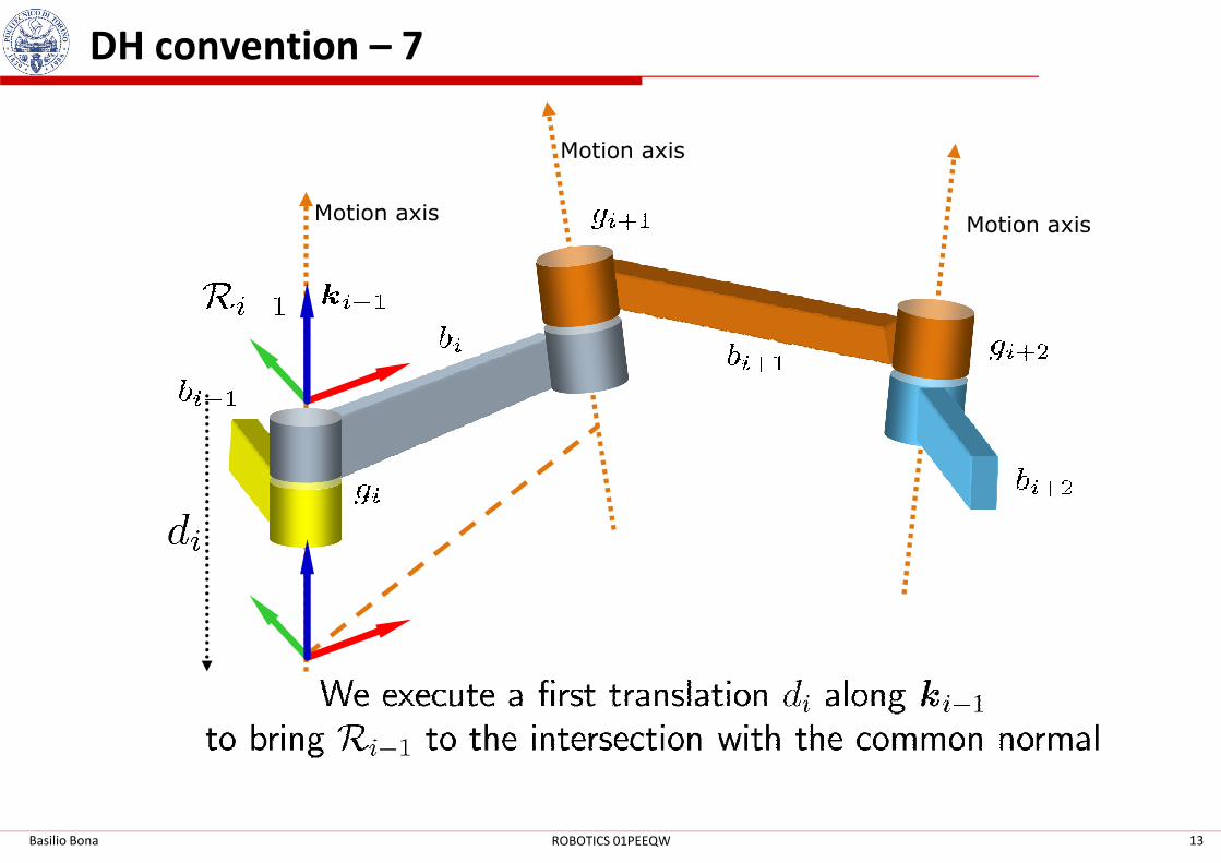
DH convention – 7
Motion axis
Motion axis
Motion axis
Basilio Bona 13ROBOTICS 01PEEQW

DH convention – 8
Motion axis
Motion axis
Motion axis
Basilio Bona 14ROBOTICS 01PEEQW

DH convention – 9
Motion axis
Motion axis
Motion axis
Basilio Bona 15ROBOTICS 01PEEQW
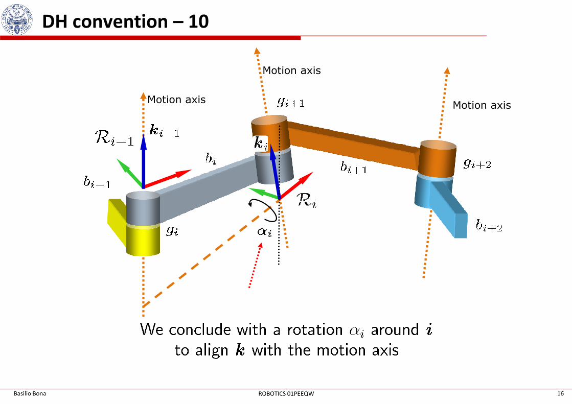
DH convention – 10
Motion axis
Motion axis
Motion axis
Basilio Bona 16ROBOTICS 01PEEQW

DH rules – 1
Basilio Bona 17ROBOTICS 01PEEQW

DH rules – 2
Basilio Bona 18ROBOTICS 01PEEQW

DH rules – 3
Basilio Bona 19ROBOTICS 01PEEQW

DH parameters
DH parameters define the transformation
1i−R iR
Depending on the joint type
ig
Basilio Bona 20ROBOTICS 01PEEQW
Prismatic joint Rotation joint
, ,i i iaθ α = fixed
( )( )i iq t d t≡
, ,i i id a α = fixed
( )( )i iq t tθ≡Joint variables
Geometrical parametersobtained by calibration

DH homogeneous roto-translation matrix
T( , )
1
= =
R tT T R t
0
cos sin cos sin sin cosaθ θ α θ α θ −
Basilio Bona 21ROBOTICS 01PEEQW
1
, ,( , ) ( , ) ( , ) ( , )i
i k iθ α
− =T T I d T R 0 T I a T R 0
1
cos sin cos sin sin cos
sin cos cos cos sin sin
0 sin cos
0 0 0 1
i i i i i i i
i i i i i i ii
i
i i i
a
a
d
θ θ α θ α θ
θ θ α θ α θ
α α−
− − =
T

From the textbook of Spong ...
Mark W. Spong, Seth Hutchinson, and M. VidyasagarRobot Modeling and ControlJohn Wiley & Sons, 2006
Basilio Bona 22ROBOTICS 01PEEQW
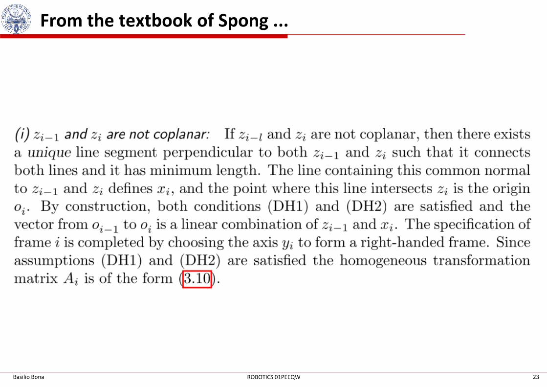
From the textbook of Spong ...
Basilio Bona 23ROBOTICS 01PEEQW

From the textbook of Spong ...
Basilio Bona 24ROBOTICS 01PEEQW

From the textbook of Spong ...
Basilio Bona 25ROBOTICS 01PEEQW

From the textbook of Spong ...
Basilio Bona 26ROBOTICS 01PEEQW

Exercise – The PUMA robot
From above
22
33
11
22 33
44
55
66
Basilio Bona 27ROBOTICS 01PEEQW
Lateral view
11
33
44 55
66
11
22
3344
5566

A procedure to compute the KFs – 1
1. Select and identify links and joints
2. Define and place the RFs using DH conventions
3. Define the constant DH parameters
4. Define the variable joint DH parameters
5. Compute the homogeneous transformation and1i
i
−T 0
TCPT
06. Extract the direct position KF from
7. Compute the inverse position KF
� Inverse velocity KF: analytical or geometrical approach
� Inverse velocity KF: kinematic singularity problem
Basilio Bona 28ROBOTICS 01PEEQW
0
TCPT

A procedure to compute the KFs – 2
1. Select and identify links and joints
2. Set all RFs using DH conventions
3. Define constant geometrical parameters
2( )q t
4( )q t
5( )q t
6( )q t
Basilio Bona 29ROBOTICS 01PEEQW
BASE
TCP
PR
0R 0PT
T
0 00 ( ) ( )( )
1P P
P
q qq = R tT0
1( )q t
6

Joint and cartesian variables
1
2
3
4
( )
( )
( )( )
( )
( )
q t
q t
q tt
q t
q t
=
q
Joint variables Task/cartesian variables/pose
1
2
3
1
2
( )
( )
( )( )
( )
( )
x t
x t
x tt
t
t
α
α
=
p
position
orientation
Basilio Bona 30ROBOTICS 01PEEQW
5
6
( )
( )
q t
q t
Direct KF
( )( ) ( )t t=p f q
2
3
( )
( )
t
t
α
α
Inverse KF
( )1( ) ( )t t−=q f p
orientation

Direct position KF – 1
position
( )
( )
1 1
2 2
3 3
4 4
5 5
6 6
( ) ( )
( ) ( )( )( ) ( )
( ) ( ( ))( ) ( )
( )( ) ( )
( ) ( )
q t p t
q t p ttq t p t
t tq t p t
tq t p t
q t p t
= ⇒ = =
x qq p q
qα
⋯
orientation
Basilio Bona 31ROBOTICS 01PEEQW
( ) ( ) ( ) ( ) ( ) ( )0 0
0 0 1 2 3 4 5 61 1 2 2 3 3 4 4 5 5 6 6 1
P P
P Pq q q q q q = =
R tT T T T T T T T
0 T
6 6( ) ( )q t p t orientation
orientation position
( )0 0 ( )P P t=R R q ( )0 0 ( )P P t=t t q

Direct position KF – 2
Direct cartesian position KF: easyeasy
110
txx t
≡ ⇔ ≡ x t
0 0
0
1P P
P
=
R tT
0 T
Basilio Bona 32ROBOTICS 01PEEQW
02 2
3 3
Px tx t
≡ ⇔ ≡ x t
Direct cartesian orientation KF:
not so not so easy easy to compute, but not difficultbut not difficult
We will solve the problem in the following slides

Direct position KF – 3
( ) ( )( ) ( )t t⇒R q qα
We want to compute angles from the rotation matrix.
But … it is important to decide which representation to use
?( )( )tqα
Basilio Bona 33ROBOTICS 01PEEQW
Euler angles
RPY angles
Quaternions
Axis-angle representation
…
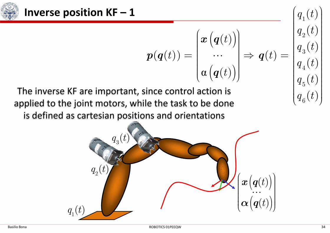
Inverse position KF – 1
( )
( )α
1
2
3
4
5
6
( )
( )( )
( )( ( )) ( )
( )( )
( )
( )
q t
q tt
q tt t
q tt
q t
q t
= ⇒ =
x q
p q q
q
⋯
The inverse KF are important, since control action is
applied to the joint motors, while the task to be done
is defined as cartesian positions and orientations
Basilio Bona 34ROBOTICS 01PEEQW
1( )q t
2( )q t
3( )q t
( )( )( )
( )
t
t
x q
q⋯
α
is defined as cartesian positions and orientations

Inverse position KF – 2
1. The problem is complex and there is no clear recipe to solve it
2. If a spherical wristspherical wrist is present, then a solution is guaranteed, but
we must find it ... how?
3. There are several possibilities
� Use brute force or previous known solutions found for similar chains
� Use inverse velocity KF (recursive approach)
� Use symbolic manipulation programs (computer algebra systems as � Use symbolic manipulation programs (computer algebra systems as
Mathematica, Maple, Maxima, …, Lisp) NOT SUGGESTEDNOT SUGGESTED
� Iteratively compute an approximated numerical expression for the
nonlinear equation (Newton method or others)
Basilio Bona 35ROBOTICS 01PEEQW
( )( )
( ){ }
1
1
1
( ) ( )
( ) ( ) 0
min ( ) ( )
t t
t t
t t
−
−
−
=
− =
−
q f p
q f p
q f p
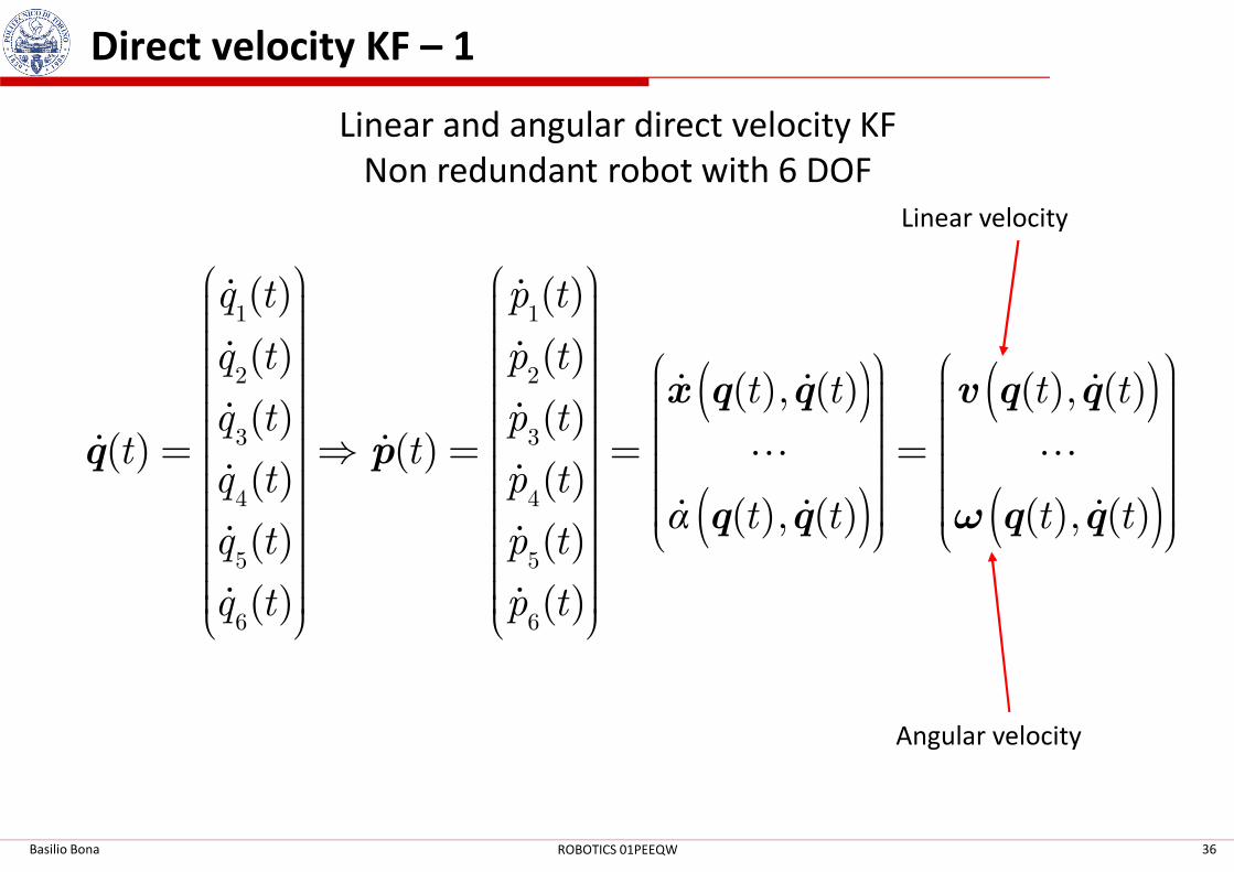
Direct velocity KF – 1
Linear and angular direct velocity KF
Non redundant robot with 6 DOF
( )1 1
2 2
3 3
( ) ( )
( ) ( )( ), ( )
( ) ( )( ) ( )
q t p t
q t p tt t
q t p tt t
= ⇒ = = x q q
q p
ɺ ɺ
ɺ ɺɺ ɺ
ɺ ɺɺ ɺ ⋯
( )( ), ( )t t =
v q qɺ
⋯
Linear velocity
Basilio Bona 36ROBOTICS 01PEEQW
( )3 3
4 4
5 5
6 6
( ) ( )( ) ( )
( ) ( )( ), ( )
( ) ( )
( ) ( )
q t p tt t
q t p tt t
q t p t
q t p t
= ⇒ = =
q p
q q
ɺ ɺɺ ɺ ⋯
ɺ ɺɺ ɺ
ɺ ɺ
ɺ ɺ
α ( )( ), ( )t t
= q qω
⋯
ɺ
Angular velocity
Direct velocity KF – 2
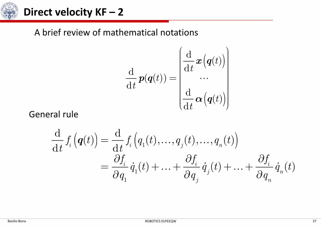
A brief review of mathematical notations
( )
( )
d( )
dd( ( ))
dd
( )d
tt
tt
tt
=
x q
p q
qα
⋯
General rule
Basilio Bona 37ROBOTICS 01PEEQW
( ) ( )1
1
1
d d( ) ( ), , ( ), , ( )
d d
( ) ( ) ( )
i i j n
i i i
j n
j n
f t f q t q t q tt t
f f fq t q t q tq q q
=
∂ ∂ ∂= + + + +∂ ∂ ∂
q … …
ɺ ɺ ɺ… …
General rule
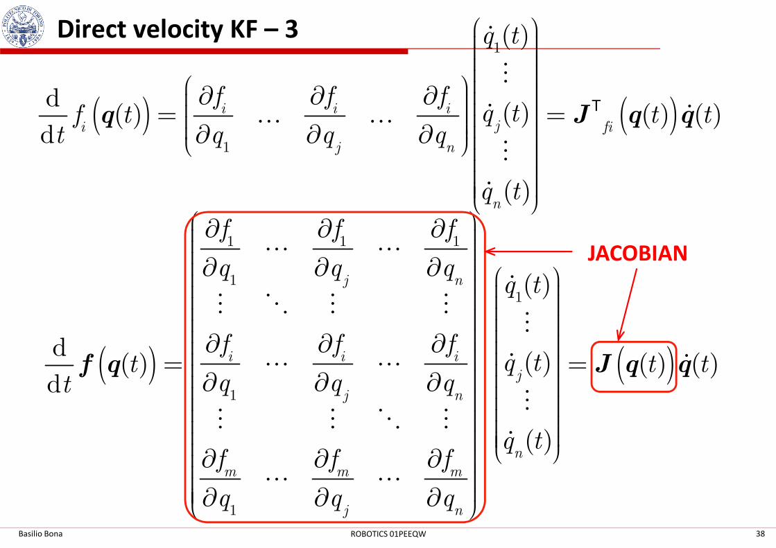
Direct velocity KF – 3
( ) ( )
1
1
( )
d( )( ) ( ) ( )
d
( )
i i iji fi
j n
n
q t
f f fq tf t t t
t q q q
q t
∂ ∂ ∂ = = ∂ ∂ ∂
q J q q
ɺ
⋮
ɺ ɺ… …
⋮
ɺ
T
1 1 1
1 ( )j n
f f f
q q qq t
∂ ∂ ∂ ∂ ∂ ∂ ⋯ ⋯
ɺ
JACOBIAN
Basilio Bona 38ROBOTICS 01PEEQW
( ) ( )
11
1
1
( )
d( )( ) ( ) ( )
d
( )
j n
i i i
j
j n
n
m m m
j n
q q qq t
f f fq tt t t
q q qt
q tf f f
q q q
∂ ∂ ∂ ∂ ∂ ∂ = = ∂ ∂ ∂ ∂ ∂ ∂ ∂ ∂ ∂
f q J q q
ɺ⋮ ⋱ ⋮ ⋮
⋮
ɺ ɺ⋯ ⋯
⋮⋮ ⋮ ⋱ ⋮
ɺ
⋯ ⋯

Velocity kinematics is characterized by Jacobians
There are two types of Jacobians:
� Geometrical Jacobian
� Analytical Jacobian
Further notes on the Jacobians
gJ
aJ
xɺ
also called Task Jacobian
The first one is related to
( )( ) ( ) ( )t t t=p J q qɺ ɺ
Basilio Bona 39ROBOTICS 01PEEQW
p g
= =
xv J q
ω
ɺɺ
a
= =
xp J q
ɺɺ ɺ
ɺα
The first one is related to
Geometrical VelocitiesGeometrical Velocities
The second one is related to
Analytical VelocitiesAnalytical Velocities

Geometrical and Analytical velocities
What is the difference between these two angular velocities?
Basilio Bona 40ROBOTICS 01PEEQW
On the contrary, linear velocities do not have this problem:
analytical and geometrical velocities are the same vector, that
can be integrated to give the cartesian position

Further notes on the Jacobians
� Moreover it is important to remember that in general no
vector exists that is the integral of ( )tu
( ) ( )( ) ( ) ( ) sin ( ) ( ) 1 cos ( ) ( ) ( )t t t t t t t tθ θ θ= + + −u u S u uωɺ ɺ ɺ
The exact relation between the two quantities is:
( )tω
?( ) ( )t t≠∫u ω
Basilio Bona 41ROBOTICS 01PEEQW
( ) ( )( ) ( ) ( ) sin ( ) ( ) 1 cos ( ) ( ) ( )t t t t t t t tθ θ θ= + + −u u S u uωɺ ɺ ɺ
While it is possible to integrate ( )tpɺ
( ) ( )( )d d
( ) ( )
t
t
ττ τ τ
τ
= =
∫ ∫x x
pɺ
ɺɺα α

Further notes on the Jacobians
� The geometrical Jacobian is adopted every time a clear
physical interpretation of the rotation velocity is needed
� The analytical Jacobian is adopted every time it is
necessary to treat differential quantities in the task space
Then, if one wants to implement recursive formula for the joint
position( ) ( ) ( )t t t t∆= +q q qɺ
Basilio Bona 42ROBOTICS 01PEEQW
1
1( ) ( ) ( ( )) ( )k k g k p kt t t t t∆−+ = +q q J q v
1
1( ) ( ) ( ( )) ( )k k a k kt t t t t∆−+ = +q q J q pɺ
or
he can use
1( ) ( ) ( )k k kt t t t∆+ = +q q qɺ

Further notes on the Jacobians
Basilio Bona 43ROBOTICS 01PEEQW

Geometric Jacobian – 1
� The geometric Jacobian can be constructed taking into
account the following steps
a) Every link has a reference frame defined according to DH
conventions
b) The position of the origin of is given by:
iR
iR
ig
1ig +
Basilio Bona 44ROBOTICS 01PEEQW
1i−R
0R
iR
1i−x
ix
1
1,
i
i i
−−r
0 1
1 1 1, 1 1,
i
i i i i i i i i
−− − − − −= + = +x x R r x r
ib

Geometric Jacobian – 2
Derivation wrt time gives
0 1 0 1
1 1 1, 1 1 1,
1 1, 1 1,
i i
i i i i i i i i i
i i i i i i
− −− − − − − −
− − − −
= + + ×= + + ×
x x R r R r
x v r
ω
ω
ɺ ɺ ɺ
ɺ
Basilio Bona 45ROBOTICS 01PEEQW
Linear velocity of wrt 1i i−R R Angular velocity of
1i−R
Remember: ( )= = ×R S R Rω ωɺ

Geometric Jacobian – 3
If we derive the composition of two rotations, we have:
0 0 1
1
0 0 1 0 1
1 1
0 1 0 1
1 1 1 1,
0 1 0 0 1
1 1 1 1, 1
( ) ( )
( ) ( )
i
i i i
i i
i i i i i
i i
i i i i i i i
i i
i i i i i i i i
−−
− −− −
− −− − − −
− −− − − − −
=
= +
= +
= +
R R R
R R R R R
S R R R S R
S R R S R R R
ɺ ɺ ɺ
ω ω
ω ω
Basilio Bona 46ROBOTICS 01PEEQW
1 1 1 1, 1
0 0
1 1 1,
( ) ( )
( ) ( )
i i i i i i i i
i i i i i
− − − − −
− − −
= + = +
S R R S R R R
S S R R
ω ω
ω ω
Hence: 0
1 1 1,i i i i i− − −= +Rω ω ω
angular velocity of RFi-1 in RF0
angular velocity of RFi in RF0 angular velocity of RFi wrt RFi-1 in RFi-1

Geometric Jacobian – 4
To compute the Geometric Jacobian, one can decompose the
Jacobian matrix as: 1
,1 ,2 , 2 3
, ,,1 ,2 ,
( ) ,L L L n
g L i A i
A A A n
n
q
q
q
= = = ∈
x J J Jv J q q J J
J J Jω
ɺ
ɺ ɺ⋯ɺ
⋯ ⋮
ɺ
R
LINEAR JACOBIAN
ANGULAR JACOBIAN
Basilio Bona 47ROBOTICS 01PEEQW
indicates how contributes to the linear velocity of the TCP
,
,1 1
d
d
L i i
n n
i L i ii ii
q
q qq= =
= =∑ ∑
J
xx J
ɺ
ɺ ɺ ɺ
indicates how contributes to the angular velocity of the TCP,1
1, ,1 1
A i
n n
i i A i ii i
q
q−
= =
= =∑ ∑
J
Jω ω
ɺ
ɺ

Structure of the Jacobian
LINEAR JACOBIAN
Basilio Bona 48ROBOTICS 01PEEQW
ANGULAR JACOBIAN

Structure of the Jacobian
If the robot is non-redundant,
the Jacobian matrix is square square
Basilio Bona 49ROBOTICS 01PEEQW
If the robot is redundant, the
Jacobian matrix is rectangularrectangular

Geometric Jacobian – 5
, 1
1,
L i i i i
i i
q d−
−
==
J k
0
ɺɺ
ω
, 1
,
L i i
A i
−==
J k
J 01i−R
R
RTCP
1i−x
xTCP
TCP1,i−r
If the joint is prismaticprismatic
If the joint is revoluterevolute
( )TCP TCP, 1, 1, 1 1,
1, 1
L i i i i i i i i
i i i i
q θ
θ
− − − −
− −
= × = ×
=
J r k r
k
ω
ω
ɺɺ
ɺ
Basilio Bona 50ROBOTICS 01PEEQW
TCP, 1 1,
, 1
L i i i
A i i
− −
−
= ×=
J k r
J k
0R
( )TCP TCP
All vectors are expresses in
is the vector that represents in
0
1, 1 0i i− −−r x x
R
R
If the joint is revoluterevolute
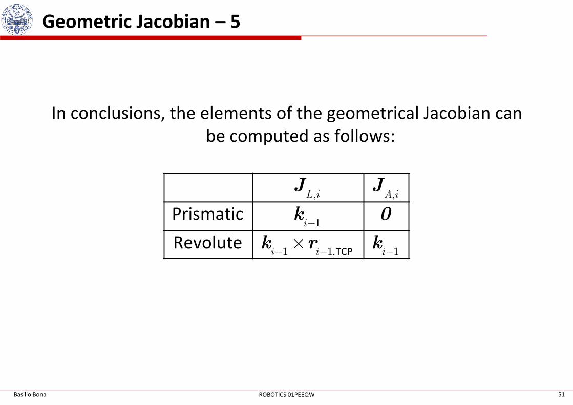
Geometric Jacobian – 5
In conclusions, the elements of the geometrical Jacobian can
be computed as follows:
Prismatic
, ,L i A iJ J
k 0
Basilio Bona 51ROBOTICS 01PEEQW
TCP
Prismatic
Revolute
1
1 1, 1
i
i i i
−
− − −×
k 0
k r k

Analytical Jacobian – 1
Analytical Jacobian is computed deriving the expression of the
TCP pose
1 1
1 11
( ( )) ( ( ))
d ( ( ))
d
d ( ( ))
n
p t p t
p qt q q
t
t
∂ ∂ ∂ ∂ = = =
q q
x q
pqα
⋯ɺ ɺ
ɺ ⋮ ⋮ ⋱ ⋮ ⋮
Basilio Bona 52ROBOTICS 01PEEQW
6 6 6
1
d ( ( ))( ( )) ( ( ))d n
n
tp p t p t qt
q q
∂ ∂ ∂ ∂
pq
q qα
⋮ ⋮ ⋱ ⋮ ⋮
ɺ ɺ⋯
( ( ))atJ q

Analytical Jacobian – 2
� The first three lines of the analytical Jacobian are equal to
the same lines of the geometric Jacobian
� The last three lines are usually different from the same
lines of the geometric Jacobian
� These can be computed only when the angle
representation has been chosen: here we consider only
EulerEuler and RPYRPY anglesEulerEuler and RPYRPY angles
� A transformation matrix relates the analytical and
geometric velocities, and the two Jacobians
Basilio Bona 53ROBOTICS 01PEEQW
( )=Tω α αɺ
( ) ( )( )g a
=
I 0J q J q
0 T α

Relations between Jacobians
� Euler angles
0 cos sin sin
( ) 0 sin cos sin
1 0 cos
φ φ θ
φ φ θ
θ
= −
T α
{ }, ,φ θ ψ=α
� RPY angles { }, ,x y zθ θ θ=α
Basilio Bona 54ROBOTICS 01PEEQW
cos cos sin 0
( ) cos sin cos 0
sin 0 1
y z z
y z z
y
θ θ θ
θ θ θ
θ
− = −
T α
The values of α that zeros the matrix T(α) determinant correspond to a
orientation representation singularityorientation representation singularity
This means that there are (geometrical) angular velocities that cannot be
expressed by joint velocities

Inverse velocity KF – 1
� When the Jacobian is a square full-rank matrix, the inverse
velocity kinematic function is simply obtained as:
( )1( ) ( ) ( )t t t−=q J q pɺ ɺ
� When the Jacobian is a rectangular full-rank matrix (i.e.,
when the robotic arm is redundant, but not singular), the
Basilio Bona 55ROBOTICS 01PEEQW
when the robotic arm is redundant, but not singular), the
inverse velocity kinematic function has infinite solutions,
but the (right) pseudo-inverse can be used to compute one
of them
( )( ) ( ) ( )t t t+=q J q pɺ ɺ
T Tdef
1( )+ −=J J JJ

Inverse velocity KF – 2
� If the initial joint vector q(0) is known, inverse velocity can
be used to solve the inverse position kinematics as an
integral
10( ) (0) ( ) d ( ) ( ) ( )
t
k k kt t t t tτ τ
+= + = + ∆∫q q q q q qɺ ɺ
Basilio Bona 56ROBOTICS 01PEEQW
0∫
Continuous time Discrete time

Singularity – 1
� A square matrix is invertible if
( )det ( ) 0t ≠J q
( )det ( ) 0St =J q
� When
Basilio Bona 57ROBOTICS 01PEEQW
a singularity exists at( )Stq
This is called a singular/singularity configuration
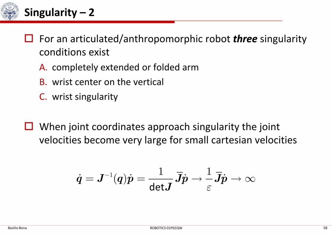
Singularity – 2
� For an articulated/anthropomorphic robot threethree singularity
conditions exist
A. completely extended or folded arm
B. wrist center on the vertical
C. wrist singularity
� When joint coordinates approach singularity the joint
velocities become very large for small cartesian velocities
Basilio Bona 58ROBOTICS 01PEEQW
det
1 1 1( )
ε
−= = → →∞q J q p Jp JpJ
ɺ ɺ ɺ ɺ

Singularity – 3
A. Extended arm
Basilio Bona 59ROBOTICS 01PEEQW
The velocities span
a dim-2 space
(the plane)
The velocities span
a dim-1 space
(the tangent line)
i.e., singularitysingularity

Singularity – 4
B. Wrist center on the vertical
these velocities cannot be
obtained with infinitesimal
joint rotations
Basilio Bona 60ROBOTICS 01PEEQW

Singularity – 5
C. Wrist singularityTwo axes are aligned
RPY wristEuler wrist
Basilio Bona 61ROBOTICS 01PEEQW
Two axes are alignedTwo axes are aligned

Euler Angles (wrist) singularity
c c s c s c s s c c s s
s c c c s s s c c c c s
s s c s c
φ ψ φ θ ψ φ ψ φ θ ψ φ θ
φ ψ φ θ ψ φ ψ φ θ ψ φ θ
ψ θ ψ θ θ
− − − + − + −
Let us start from the symbolic matrix3 angles
Basilio Bona 62ROBOTICS 01PEEQW
Observe that if 1 0cθ
θ= ⇒ =
0
0
0 0 1
c c s s c s s c
s c c s c c s s
φ ψ φ ψ φ ψ φ ψ
φ ψ φ ψ φ ψ φ ψ
− − − + − cos( )φ ψ+
sin( )φ ψ+
1 angle
only
we have

Singularity
� In practice, when the joints are nearnear a singular
configuration, to follow a finite cartesian velocity the joint
velocities become excessively large
� Near singularity conditions it is not possible to follow a
geometric path and at the same time a given velocity
profile; it is necessary …
� to reduce the cartesian velocity and follow the path, or� to reduce the cartesian velocity and follow the path, or
� to follow the velocity profile, but follow an approximated
path
� In exact singularity conditions, nothing can be done … so …
avoid singularityavoid singularity
Basilio Bona 63ROBOTICS 01PEEQW

Conclusions
� Kinematic functions can be computed once the DH
conventions are applied
� Inverse position KF is complex
� Direct velocity KF has the problem of angular velocities:
analytical vs geometric Jacobiansanalytical vs geometric Jacobians
� Inverse velocity can be computed apart from singularity
points
� Avoid singularities
Basilio Bona 64ROBOTICS 01PEEQW


![Robot Dynamics & Control - University of Queenslandrobotics.itee.uq.edu.au/~metr4202/2013/lectures/L4-Dynamics.v1.pdf · 4 16-Aug Robot Dynamics & Control ... Denavit Hartenberg [DH]](https://static.fdocuments.us/doc/165x107/5a8794817f8b9a882e8dbf53/robot-dynamics-control-university-of-metr42022013lecturesl4-dynamicsv1pdf4.jpg)


![arXiv:1711.03808v1 [cs.RO] 10 Nov 2017 · Servo Motor, PWM, Homogenous Transformations, Kinematic Chain, Denavit { Hartenberg Parameters, Schematic, Datasheet, Consumptions, Java-C++-C,](https://static.fdocuments.us/doc/165x107/5ec09c6fcb76bc13d41dde72/arxiv171103808v1-csro-10-nov-2017-servo-motor-pwm-homogenous-transformations.jpg)