Robotic Sanding of Wooden Bowls with Hybrid

Force/Position Impedance Control

by

Srijith Sudhagar

A thesis submitted in conformity with the requirements for

the degree of Master of Applied Science

in the

Faculty of Engineering and Applied Science

Department of Mechanical and Materials Engineering

QUEEN’S UNIVERSITY

Kingston, Ontario, Canada

January 2020

Copyright © Srijith Sudhagar, 2020

ii

ABSTRACT

Srijith Sudhagar: Robotic Sanding of Wooden Bowls with Hybrid Force/Position Impedance

Control. MASc. Thesis, Queen’s University, January 2020.

This thesis set out to determine whether a serial robot could be used to sand a wooden bowl, in

order to free a human operator from what is considered a hazardous task. The process of sanding

wood is similar to the polishing of metal, both set out to eliminate scratches. There are robot-based

commercial systems available for the polishing of metal, for example aluminum, as employed by

the aerospace industry. However, unlike aluminum, wood is a non-homogeneous material. In the

case of wooden bowls, each has a unique geometry, and to a degree, unique material properties.

The hypothesis posed by this thesis is that a hybrid force/position impedance controller can sand

the inside of a wooden bowl and mimic the motions and technique of a human operator, and yet

be able to deal with conditions of unknown bowl geometry.

A CRS A465 robotic arm was used to mimic the arm motion of a human operator. The bowl was

held in place by a vacuum chuck. A pneumatic orbital sander was used for the sanding process. A

3-axis force sensor mounted on the end effector measured the applied force. The arm was

programmed to follow a radial line from the rim of the bowl to its center and then back to the rim.

A hybrid force/position impedance controller was implemented. A forward and inverse kinematic

model of the robot was developed to enable trajectory generation. The effect of sander angle and

the nature of the trajectory was tested. PD action was adopted for the position controller. Four

different force controllers were tested: First Order (FO) filter, Butterworth filter, PI action and

combined FO/PI. Tuning tests were conducted to obtain the best values for the controller gains.

The conclusion is that a FO filter for the force controller and PD action for the position controller,

with an appropriate settings for the impedance, gave the best control performance. This

performance was obtained with only a rough estimation of the bowl geometry as based on the

bowl’s diameter and depth. A precise CAD/CAM model of the bowl was not employed.

iii

ACKNOWLEDGEMENTS

I would like to express my deepest gratitude to my supervisor, Dr. Brian Surgenor for his full

support, expert guidance, understanding and incredible patience throughout my study and research.

I have learned a lot from him throughout the completion of this thesis work.

I would also like to thank my co-supervisor Prof. Keyvan Hashtrudi-Zaad and PdF. Chiedu

Mokogwu for helping me to set up the CRS robot and force sensor. I would like to acknowledge

the work of my friend: Hamza Sheikh. Thank you for your help with transferring inverse kinematic

equations to the Simulink. I thank my lab mates Victor Luna, Andres Ramos, Shane Forbrigger

and Orighomisan Mayuku for their support with moving equipment and testing of the robot. Thank

you all for your helpful ideas, enthusiasm and friendship during the last two years.

The financial support provided by the School of Graduate Studies and Department of Mechanical

and Materials Engineering is greatly acknowledged.

I must express my gratitude for my parents, my brother and my friends, without whose support I

would not have been able to reach this important moment of my life. Finally, I thank Queen’s and

Kingston on the whole for making my two years stay here a most enjoyable and valuable time of

my life.

iv

TABLE OF CONTENTS

TITLE PAGE

ABSTRACT ii

ACKNOWLEDGEMENTS iii

TABLE OF CONTENTS iv

LIST OF FIGURES vii

LIST OF TABLES xi

LIST OF NOMENCLATURE xii

Chapter 1 INTRODUCTION 1

1.1 Problem Overview 1

1.2 Objectives 3

1.3 Thesis Outline 4

Chapter 2 LITERATURE REVIEW 6

2.1 Robot Based Polishing and Sanding 6

2.1.1 Tool on the Robot 6

2.1.2 Workpiece on the Robot 7

2.1.3 Two Robot Setup 8

2.1.4 Tool Path Planning 8

2.2 Kinematic and Dynamic Modelling 9

2.3 Hybrid Force/Position Control 11

2.4 Impedance Control 13

2.5 Filters for Force Control 14

2.6 Summary 14

Chapter 3 APPARATUS AND CONTROLLERS 16

3.1 Articulated Robot 16

3.1.1 CRS A465 Arm 17

3.1.2 C500C Controller 19

3.1.3 Teach Pendant 20

3.1.4 Computer Software 22

3.2 Force Sensor 23

3.3 Trajectory Planning 27

3.4 Orbital Sander 28

3.5 Vacuum Chuck 30

v

3.6 Controllers 31

3.6.1 PI Force Control 32

3.6.2 First Order Filter 33

3.6.3 Butterworth Filter 33

3.6.4 FOPI Force Control 34

3.7 Summary 34

Chapter 4 KINEMATICS AND DYNAMICS 35

4.1 DH Parameters 35

4.1.1 Transformation Matrices 37

4.2 Forward Kinematics 39

4.3 Inverse Kinematics 40

4.4 Differential Kinematics 47

4.5 Robot Dynamics 49

4.5.1 Lagrange 49

4.5.2 Mass and Inertia Terms 51

4.5.3 Coriolis and Centrifugal Terms 52

4.5.4 Gravitation and Friction Terms 53

4.5.5 Force Estimation 54

4.5.6 Parametrization 54

4.6 Summary 55

Chapter 5 RESULTS 56

5.1 FO/PD Control Results 58

5.1.1 Impedance Factor 58

5.1.2 Effect of Contact Angle 62

5.1.3 Effect of Trajectory 65

5.1.4 BTU and No Contact 68

5.1.5 BTU and Integral Action 70

5.1.6 Tuned FO/PD Control 72

5.2 BW/PD Control Results 75

5.3 PI/PD Control Results 76

5.4 FOPI/PD Control Results 81

5.5 Comparison of Tuned Results 84

5.6 Summary 87

Chapter 6 CONCLUSIONS AND RECOMMENDATIONS 88

6.1 Conclusions 89

6.2 Contributions 89

6.3 Recommendations 90

vi

REFERENCES 91

APPENDIX A - Hardware Specifications 94

APPENDIX B - Dynamics Equations 98

APPENDIX C - Simulink Blocks 101

APPENDIX D - Tuning Plots 111

APPENDIX E - MATLAB Code 119

vii

LIST OF FIGURES

2.1 “Symmetrical offset linear” tool path. 9

2.2 Force analysis of tool head polishing on curved surfaces. 9

2.3 Coordinate frame assignment of the CRS A465 arm. 11

2.4 Hybrid force/position controller. 12

2.5 Impedance control scheme. 14

2.6 Position based impedance controller block diagram. 14

3.1 Workspace setup of the CRS A465 arm (left) and XYZ axes orientation (right). 17

3.2 Joint positions of CRS A465. 18

3.3 Home (left) and ready (right) positions of the arm. 19

3.4 C500C controller box with the PC and teach pendant visible. 20

3.5 Teach pendant. 21

3.6 Simulink block diagram with implementation of the hybrid controller. 22

3.7 Force sensor axes orientation (JR3). 24

3.8 1kg weight placed on the z axis of the sensor. 24

3.9 Change in Fz when 1kg weight placed on z axis, with Fx and Fy constant. 25

3.10 Arrangement for loading the x axis of the sensor with 1kg weight. 25

3.10 Plot of recorded force versus applied force. 26

3.11 Dimensions of the bowl in mm. 27

3.12 Sander with a 30 deg contact angle. 27

3.13 Adapter plate for mounting sander to the wrist. 28

3.14 Close-up of the end effector, showing mount of the orbital sander and

force sensor. 29

3.15 Illustration of applied forces by sander in x and z direction. 29

3.16 Vacuum chuck connected to the vacuum pump with bowl sitting on the chuck. 30

3.17 Block diagram of hybrid force/position controller. 32

viii

4.1 Denavit-Hartenberg diagram of the CRS A465 arm. 37

5.1 Placement of event markers for sander entry and return paths. 57

5.2 Sample force plot as keyed to event markers, with setpoints of 0 and -14N

for Fx and Fz. 57

5.3 Sample position error plot as keyed to event markers. 57

5.4 Position error for X axis with FO/PD control and effect of Kt. 60

5.5 Position error for Z axis with FO/PD control and effect of Kt. 60

5.6 Force error for X axis with FO/PD control and effect of Kt. 61

5.7 Force error for Z axis with FO/PD control and effect of Kt. 61

5.8 Position error for X axis with FO/PD control and effect of contact angle. 63

5.9 Position error for Z axis with FO/PD control and effect of contact angle. 63

5.10 Force error for X axis with FO/PD control and effect of contact angle. 64

5.11 Force error for Z axis with FO/PD control and effect of contact angle. 64

5.12 Two types of trajectories used for testing. 66

5.13 Force result for Trajectory 1 with FO/PD control. 67

5.14 Force result for Trajectory 2 with FO/PD control. 67

5.15 Position error for X axis showing effect of sanding. 69

5.16 Position error for Z axis showing effect of sanding. 69

5.17 Ball transfer unit (BTU). 70

5.18 Force error with FO/PD hybrid controller and BTU. 71

5.19 Force error with FOPI/PD hybrid controller and BTU. 71

5.20 Position error for X and Z axis with tuned FO/PD control. 73

5.21 Force result for X and Z axis with tuned FO/PD control. 73

5.22 Force error for Z axis with FO/PD control and repeated trials. 74

5.23 Force error for X axis with PI/PD control and tuning of KP for force. 77

5.24 Force error for Z axis with PI/PD control and tuning of KP for force. 77

5.25 Force error for X axis with PI/PD control and tuning of KP for force

(filtered data). 78

5.26 Force error for Z axis with PI/PD control and tuning of KP for force

ix

(filtered data). 78

5.27 Force error for X axis with PI/PD control and tuning of KI for force. 79

5.28 Force error for Z axis with PI/PD control and tuning of KI for force. 79

5.29 Force error for X axis with PI/PD control and tuning of KI for force

(filtered data). 80

5.30 Force error for Z axis with PI/PD control and tuning of KI for force

(filtered data). 80

5.31 Position error for X axis with different force controllers. 82

5.32 Position error for Z axis with different force controllers. 82

5.33 Force error for X axis with different force controllers. 83

5.34 Force error for Z axis with different force controllers. 83

5.35 Comparison of position and force error (X and Z axes) of the tuned results. 84

5.36 Position error for X axis comparing tuned result of controllers. 85

5.37 Position error for Z axis comparing tuned result of controllers. 85

5.38 Force error for X axis comparing tuned result of controllers. 86

5.39 Force error for Z axis comparing tuned result of controllers. 86

A.1 Husky 15.2cm disc orbital sander. 94

A.2 Bosch orbital sander. 95

A.3 JUN-AIR compressor. 96

A.4 Shop drawing for adapter plate. 97

C.1 Simulink model used to program the A465 arm. 102

C.2 Blocks used to input the trajectory in world coordinates. 103

C.3 Sub-blocks inside the inverse kinematics block. 103

C.4 Sub-blocks used in the position control block. 104

C.5 Sub-blocks inside the Closed loop block of joint 1. 105

C.6 Sub-blocks inside the Joint 1 block. 105

C.7 Sub-blocks inside the PD controller1 block. 106

x

C.8 Sub-blocks inside the Force control block in main Simulink model. 106

C.9 Sub-blocks inside the FO filter block. 107

C.10 Sub-blocks inside the PI controller block. 107

C.11 Sub-blocks inside the Butterworth filter block. 108

C.12 Blocks present in CRS_takeover block which is used to switch between

OA and CRS mode of the arm. 108

C.13 Sub-blocks inside the angle to coordinates block. 108

C.14 Sub-blocks in encoder readings block used to compare the actual and

desired trajectory. 109

C.15 Sub-blocks in home block. 110

C.16 The sub-blocks included in the forward kinematics block. 110

D.1 Position error for X axis with FO/PD control and tuning of time constant. 112

D.2 Position error for Z axis with FO/PD control and tuning of time constant. 112

D.3 Force error for X axis with FO/PD control and tuning of time constant. 113

D.4 Force error for Z axis with FO/PD control and tuning of time constant. 113

D.5 Position error for X axis with BW/PD control and tuning of Pf. 114

D.6 Position error for Z axis with BW/PD control and tuning of Pf. 114

D.7 Force error for X axis with BW/PD control and tuning of Pf. 115

D.8 Force error for Z axis with BW/PD control and tuning of Pf. 115

D.9 Position error for X axis with PI/PD control and tuning of KP for position. 117

D.10 Position error for Z axis with PI/PD control and tuning of KP for position. 117

D.11 Position error for X axis with PI/PD control and tuning of KD for position. 118

D.12 Position error for Z axis with PI/PD control and tuning of KD for position. 118

ii

LIST OF TABLES

3.1 Calibration matrix as supplied by JR3 for this particular unit. 24

3.2 Correction factors for respective masses in Fz axis. 25

4.1 DH parameters for all six joints of CRS A465 arm. 36

5.1 Control parameters for RMSE results for hybrid FO/PD controller. 59

5.2 Results for change in angle with hybrid FO/PD controller. 62

5.3 Results for change in trajectory with hybrid FO/PD controller. 65

5.4 Results with change in contact and FO/PD controller. 68

5.5 Results with FO/PD and FOPI/PD controllers. 70

5.6 Best result with hybrid FO/PD controller. 72

5.7 Results for repeated trials with hybrid FO/PD controller. 74

5.8 Control parameters for hybrid BW/PD controller. 75

5.9 Tuning results of KPf for hybrid PI/PD controller. 76

5.10 Tuning results of KIf for hybrid PI/PD controller. 76

5.11 Comparison of PI/PD and FOPI/PD controllers. 81

5.12 Tuned set of control parameters for different controllers. 84

D.1 Tuning time constant (𝜏) for hybrid FO/PD controller. 111

D.2 Tuning results of KPp for PD controller. 116

D.3 Tuning results of KDp for PD controller. 116

iii

LIST OF NOMENCLATURE

ai link length of ith joint

𝑎𝑏𝑎 approach vector between Frame a and Frame b

A2 length of link 2

ci cosine of ith joint angle

di joint offset of ith joint

D4 length of link 3

𝐸𝑝𝑥, 𝐸𝑝

𝑧 position error in x and z axis

𝐸𝑓𝑥, 𝐸𝑓

𝑧 force error in x and z axis

Fc cutoff frequency

Fx,Fz force measured in x an z axis

fp passband frequency

f measured force

fv viscous friction

fc coulomb friction

J jacobian

KE kinetic energy

KD derivative gain

KI integral gain

Kp Attenuation at passband frequency

KP proportional gain

Kt impedance factor

𝑛𝑏𝑎 normal vector between Frame a and Frame b

PE potential energy

px, py, pz change in position in x, y and z axis

q joint angle

ri change in orientation

Si Setpoint

𝑠𝑏𝑎 slide vector between Frame a and Frame b

si sine of ith joint angle

iv

𝑝𝑏𝑎 position vector between Frame a and Frame b

𝑇60 final transformation matrix

v linear velocity

V voltage applied to the motor

Zm mechanical impedance

Acronyms

BUFD Backward-Up/Forward-Down

BW Butterworth

CSG Constructive Solid Geometry

CAD Computer-Aided Design

CAM Computer-Aided Manufacturing

DH Denavit-Hartenberg

DSP Digital Signal Processing

DOF Degrees of Freedom

FO First Order

FUBD Forward-Up/Backward-Down

HIL Hardware in Loop

OA Open Architecture

PBIC Position Based Impedance Control

PCI Peripheral Component Interconnect

PET Polyethylene Terephthalate

PD Proportional-Derivative

PI Proportional-Integral

PID Proportional-Integral-Derivative

RMSE Root Mean Square Error

BTU Ball Transfer Unit

v

Greek Letters

αi link twist of ith joint

Θi joint angle of ith joint

𝜔𝑖 angular velocity of ith joint

𝜔𝑐 cut off frequency

𝜏 time constant

1

CHAPTER 1

INTRODUCTION

In certain woodworking industries, human operators manually cut wooden bowls and then sand

them with electric hand-held power sanders. This is a physically demanding process and frequently

leads to carpal tunnel injuries of the wrist [1]. Automating the wood sanding process could lead to

increased production rates and free operators from a hazardous work environment. The process of

sanding wood is similar to the polishing of metal, both set out to eliminate scratches. There are

robot-based commercial systems available for the polishing of metal, for example aluminum, as

employed by the aerospace industry [2]. However, unlike aluminum, wood is a non-homogeneous

material. In the case of wooden bowls, each has a unique geometry, and to a degree, unique

material properties. The hypothesis posed by this thesis is that a hybrid force/position impedance

controller could match the performance of a human operator and still be able to deal with the

conditions of unknown bowl geometry.

In the next section, a problem overview is given of the hazardous and difficult nature of the sanding

process. The problem overview section is followed by a section that lists the main objectives of

the thesis. In the last section of this chapter, the thesis outline is given.

1.1 Problem Overview

In the production of wooden bowls, one approach taken by a local manufacturer is to first make a

rough cut of the bowl from a tree trunk using a lathe. Initial sanding of the inner surface is then

conducted using a large belt sander, with the operator sitting in a chair and holding the bowl against

the sander, which is mounted on the floor. Final sanding of the bowl is accomplished by holding

the bowl horizontally in a fixture and having the operator conduct continuous passes of a handheld

powered orbital sander. There are a number of risks associated with this process:

2

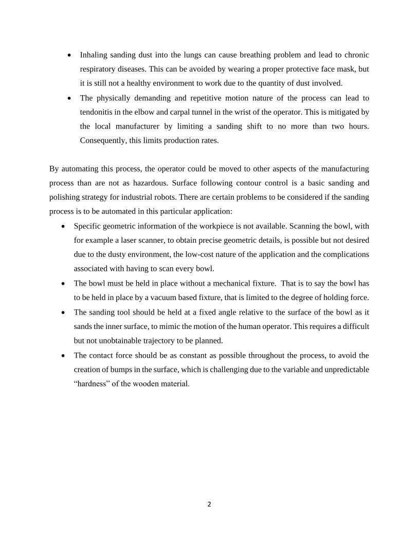
• Inhaling sanding dust into the lungs can cause breathing problem and lead to chronic

respiratory diseases. This can be avoided by wearing a proper protective face mask, but

it is still not a healthy environment to work due to the quantity of dust involved.

• The physically demanding and repetitive motion nature of the process can lead to

tendonitis in the elbow and carpal tunnel in the wrist of the operator. This is mitigated by

the local manufacturer by limiting a sanding shift to no more than two hours.

Consequently, this limits production rates.

By automating this process, the operator could be moved to other aspects of the manufacturing

process than are not as hazardous. Surface following contour control is a basic sanding and

polishing strategy for industrial robots. There are certain problems to be considered if the sanding

process is to be automated in this particular application:

• Specific geometric information of the workpiece is not available. Scanning the bowl, with

for example a laser scanner, to obtain precise geometric details, is possible but not desired

due to the dusty environment, the low-cost nature of the application and the complications

associated with having to scan every bowl.

• The bowl must be held in place without a mechanical fixture. That is to say the bowl has

to be held in place by a vacuum based fixture, that is limited to the degree of holding force.

• The sanding tool should be held at a fixed angle relative to the surface of the bowl as it

sands the inner surface, to mimic the motion of the human operator. This requires a difficult

but not unobtainable trajectory to be planned.

• The contact force should be as constant as possible throughout the process, to avoid the

creation of bumps in the surface, which is challenging due to the variable and unpredictable

“hardness” of the wooden material.

3

1.2 Objectives

There are five main objectives for this thesis project:

1) Develop a robot-based apparatus to test the feasibility of sanding a wooden bowl.

Identify and commission an appropriate robotic arm with a force sensor and a sander as the

end effector.

2) Develop a controller for the apparatus.

A hybrid controller should be designed to achieve both position and force control as the

sander is drawn across the surface of a wooden bowl.

3) Implement and validate a model of the robotic arm.

Derive and test a kinematic and dynamic model of the robotic arm to enable trajectory

planning and execution.

4) Determine the control performance possible through experimentation.

Perform sanding tests and monitor the results as the controllers are tuned.

5) Analyze the results of the sanding tests and identify potential areas for improvement.

If possible, make modifications to the apparatus to improve performance, as suggested by

the outcomes of the sanding tests.

Tasks to be completed to achieve these objectives:

In order to achieve these objectives, the following tasks will be completed.

1. Confirm the operation of the robotic arm with a teach pendant and its dedicated controller.

When in closed architecture mode, the basic operation of the robot can be confirmed with

a teach pendant, to enable any necessary hardware debugging.

2. Connect the robot’s controller to a computer and run the arm in open architecture mode.

In order for the robot to be operated in open architecture mode (i.e. controlled by a desktop

computer), the hardware interface between the computer and the dedicated controller must

be rendered operational.

3. Study the kinematics and derive the dynamic equations for the robot. A kinematic model

is needed in order to program the robot for user defined motions.

4. Install and calibrate a 3-axis force sensor for mounting on the robot’s end effector. The

force sensor needs to be calibrated with static weights before mounting on the arm.

4

5. Install a device to hold the wooden bowl in place during the sanding process, without

damaging in the bowl (i.e. the bowl can’t be drilled out for bolt mounts). A suitably sized

vacuum chuck should be used to hold the bowl, with chuck mounted on a table, at the same

level as the base of the robot’s arm.

6. Install and test an appropriate sander. The manual sanding of a bowl is conducted with

two types of sanders: electric belt and electric orbital. Both are too heavy and too large to

be used at the end of a robotic arm. A lighter and smaller sander must be found.

7. Review the literature for the structure of an appropriate hybrid force/position controller.

The hybrid controllers used by other researchers for the sanding of wood (and the polishing

of metal) should be studied and an appropriate structure chosen for the application at hand.

8. Implement the candidate controller and investigate the operating parameters that influence

the quality of the sanding process. A number of operating parameters need to be identified

including angle of the sander, nature of the sanding motion (trajectory planning),

magnitude of the force setpoint, speed of the sanding process and finally, the controller

gains need to be tuned.

1.3 Thesis Outline

Chapter 2 presents background information and provides a literature review on the subject of the

polishing of metal and the sanding of wood with a robot. The experience of other researchers when

it comes to hybrid force/position controller is examined. Attention is also given to the problem of

contour following when dealing with curved surfaces. The availability of existing kinematic and

dynamic robot models is presented, with a focus on models that are sufficiently well documented

to enable implementation for this thesis. The importance of including impedance control is

confirmed. Details such as the need for filtering when working with a force controller are reviewed.

Finally, lessons learned from the literature review are summarized.

Chapter 3 provides details on the assembled apparatus, including the robotic arm and its dedicated

controller. The software needed to control the arm with a desktop computer is discussed. The

specifications of the selected force sensor and the adopted calibration method are given. Details

5

of the selected sander are presented. Finally, the four different controller configurations selected

for testing are documented.

Chapter 4 explains the derivation of the kinematic and dynamic model used to enable control of

the robot. The DH parameters of the arm are first given, followed by the derivation of the

transformation matrices. Next, the forward and inverse kinematic equations are developed.

Jacobians are used to formulate the dynamic equations. Model specifics are presented, including

inertia terms, coriolis and centrifugal terms, gravitational and frictional terms. Finally, the force

estimation and parametrization equations are given.

Chapter 5 presents the results of the sanding tests with four different hybrid controllers and under

different operating conditions. Trajectory planning was validated by tracking the motion of the

arm without the wooden bowl present. The effect of friction was examined by replacing the sander

with a ball transfer unit, that is to say the sander was replaced by a sprung ball bearing that rolled

freely on the surface of the wooden bowl. Empirical tuning tests were conducted to tune the gains

of all four controllers. The effect of changing the trajectory and the sander’s orientation is

presented. Finally, a comparison is given of the best results from each controller.

Chapter 6 concludes the thesis, summarizing the work done and the significance of the test results

obtained. Recommendations for future work are presented. Reflections are given on the feasibility

of automating the sanding process for wooden bowls

6

CHAPTER 2

LITERATURE REVIEW

As introduced in Chapter 1, the overall objective of this thesis is to develop a robot-based apparatus

to test the feasibility of sanding a wooden bowl. This chapter begins with a review of robot-based

polishing of metal and the sanding of wood. Previous research on the subject of hybrid

force/position control with robotic arms is examined. The problem of contour following when

dealing with curved surfaces is reviewed. The availability of existing kinematic and dynamic robot

models is surveyed, with a focus on models that are sufficiently well documented that they could

be readily applied to the problem addressed by this thesis. The significance of impedance control

is examined. The need for filtering when working with a force controller is presented. Finally,

lessons learned from the literature review are summarized.

2.1 Robot-Based Polishing and Sanding

As will be described in the following three sub-sections, robot-based sanding and polishing can be

conducted in one of three ways. Unless stated otherwise, the robots in the reviewed papers are

articulated serial arms with six degrees of freedom (DOF) that is to say, with six revolute joints.

2.1.1 Tool on the Robot

The papers in this section have the tool mounted on the robot and the workpiece held stationary.

A number of studies have been conducted on the polishing of metal, but only a few can be found

on the sanding of wood. One early study of robotic polishing with industrial robot was completed

by Takeuchi et al. [3] where an air-driven spindle was used to a polish a broad planar metal surface.

In this study, a touch sensor on the robot arm was used to obtain the location of the workpiece on

the table and the information was stored as Constructive Solid Geometry (CSG) data. This CSG

7

data was then used by a CAD/CAM system to calculate the normal vector and feed vector at each

point on the workpiece surface. Thus, performance in this study was predicated by the need for

precise information on the geometry of the workpiece.

A similar CAD/CAM based approach was taken by Nagata et al. [4] for a metal mold polishing

robot (articulated industrial arm) where a ball-end abrasive tool was used to polish PET

(Polyethylene Terephthalate) bottle molds. The target tool location and vector data were used to

provide not only the desired trajectory of the tool but also the desired contact orientation. They

used a hybrid controller where the position control loop fed into to the force control loop to achieve

both accurate pick and place feed control of the tool position and stable force control.

Another CAD/CAM based approach was taken by Nagata et al. [5] where industrial robot equipped

with an orbital sander was used to sand furniture with free-formed curved surfaces. The key feature

of their system is that the sanding force acting between the tool and the wooden workpiece was

precisely controlled to track a target force. On the other hand, even though the workpiece geometry

was known precisely, process parameters such as control gains were tuned by trial and error

method.

To avoid collision between the polishing tool and the workpiece, the arm should be guided with

collision free CSG data based on recognition and judgement like human operator. This was studied

by Takeuchi et al. [6] using polishing robot with electric (convex end) tool to polish a carbon steel

concave surface. A collision free polishing tool path was generated to obtain uniform surface finish

throughout the workpiece.

2.1.2 Workpiece on the Robot

The paper in this section has the workpiece mounted on the robot and the tool is held stationary.

An alternative method for the robotic polishing of complex curved surfaces is known as the top

down approach. This approach was studied by Mohsin et al. [7] who used an articulated robot for

the polishing of eyeglass frames. In this method, the robot holds the workpiece and the polishing

8

disc is fixed onto a base. The complex curved surface is broken down into a number of simple

curved surfaces for polishing. The tool path is generated for each surface region and then the

regions are stitched together. They achieved a high-quality surface with all scratches eliminated in

just two polishing cycles.

2.1.3 Two-Robot Setup

The paper in the section has the tool mounted on the robot and the workpiece on a second robot

(or rather a machine tool with 3 DOF).

Common approach is to mount the sanding/polishing tool on the robot and have the workpiece

fixed in place. Another approach is to have workpiece on a machining center with one or more

axes and a polishing robot with two or more axes. For example, a study completed by Cheol Lee

et al. [8] used three axis machining center and two axis polishing robot equipped with an air driven

tool to polish on shadow mask die. They used DSP (Digital Signal Processing) controller to obtain

precise polishing.

2.1.4 Tool Path Planning

The automated polishing of metal on curved surfaces was discussed in Tian et al. [9], [10]. They

used an industrial robot with a flexible abrasive tool to polish a curved mold surface. In [9], tool

path planning was done with a symmetrical offset line feed style as illustrated in Figure 2.1. Taking

the center line as the axis of symmetry, two sides of the workpiece symmetrically extend according

to the preset cutter row spacing, until the path is complete.

9

Figure 2.1: “Symmetrical offset linear” tool path [9].

Gravity compensation of the polishing tool plays an important role in polishing. In Tian et al.’s

approach [10], the relation between the polishing force and the effect of gravity on the tool was

taken into account and the polishing process was studied. They proposed an algorithm from the

real-time polishing force detection to the normal polishing force based on the force analysis and

gravity compensation on the polishing tool. It was then used to decrease the influence by polishing

tool gravity and improve the real time control of the normal polishing force accurately. And which

was then used to decrease the influence of gravity and improve the real time control of the normal

polishing force. Force analysis of the tool head is illustrated in Figure 2.2 where Fn is the normal

force, Fm is the force measured using the sensor, Fg is the polishing tool gravity and Fc is the

polishing force.

Figure 2.2: Force analysis of tool head polishing on curved surfaces [10].

10

Polishing based on analysis of the contact force and path research was completed by Huang et al.

[11], where they used an industrial robot with electric buffing wheel for turbine blade polishing

(one of the main components in an aircraft engine). The width of the contact surface was obtained

and then it was used to optimize the polishing path. Later they applied the contact force analysis

to flexible robot polishing system to achieve high quality.

2.2 Kinematic and Dynamic Modelling

The forward and inverse kinematics of the robot arm are required for end point control and

identification of associated dynamic parameters.

The Denavit-Hartenberg (DH) parameters are important to provide the forward and inverse

kinematic calculations. These parameters describe the arm mathematically which is explained in

“Robotic Analysis” by Tsai, L. [12]. After deriving all the DH parameters for six joints, the

transformation matrices need to be computed to describe the relationship between two joint frames.

The frames of the arm are shown in Figure 2.3 where the first joint is considered as Frame 1. Then

the forward and inverse kinematic equations are formulated from these transformation matrices.

This approach will be covered in detail in Chapter 4 of thesis.

In order to design a controller for a robot, a precise model of the robotic system is required with

accurate information on dynamic parameters. The manual provided by the CRS did not contain

data about the inertial parameters such as link mass, moment of inertia, center of mass and joint

friction. These are needed to design model-based controllers. The dynamic model was derived by

Kinsheel et al. [13] used the Lagrange Euler method for force estimation which includes

components such as manipulator mass matrix, inertia of the actuators, vector of coriolis and

centrifugal terms, vector of gravitational forces, coulomb friction, viscous friction, end-effector

torque, controller gain, input voltage and gear ratio of the motors.

11

Figure 2.3: Coordinate frame assignment of the CRS A465 arm [13].

The trajectories for each joint were generated using Fourier series and fed into the robot controller

to collect two sets of identification data, one at full speed and the other at half speed. Radkhah et

al. [14] set out to identify the dynamic parameters of a CRS A460 robot. Fourier series parameters

were used to generate the joint trajectories to identify the dynamic parameters. The data included

the measured position of joints from encoders and recorded command voltages from the controller

output. Data processing was done by taking the average of each joint position. The parameters

were computed by the pseudoinverse method (i.e. unweighted least squares). Finally, the force

exerted by the end-effector was estimated by collecting the voltage output from the force sensor

and converting them into newtons.

2.3 Hybrid Force/Position Control

In this section, advanced control algorithms used for robot based polishing and sanding are

reviewed. Advanced approaches combine traditional force only control methods with advanced

control algorithms such as adaptive, robust and learning control strategies.

12

An overview of different types of robot force controllers was given by Zeng et al. [15]. An essential

undertaking in robot force control is how to determine the interaction forces and effectively utilize

the feedback signals in order to synthesize the required input signals, so that the desired motion

and force can be maintained. Force control methods like stiffness control, impedance control,

admittance control and hybrid force/position control were studied. In hybrid force/position control,

a position controller is run in parallel (or in series) with a force controller. Figure 2.4 shows the

parallel configuration. In one specific example, PI was used for the force controller and PD for the

position controller [15]. In this way, the position control has a fast response (D action) and the

force control acts to minimize steady state error (I action). The papers discussed in previous section

used either hybrid force/position control, impedance control or a combination of both.

In reference to figure 2.4, the command torque (𝜏) is obtained by adding the torque output from

the position and force controllers. Position and force are fed back into their respective controllers

for tracking. S and I-S are the function blocks of a differentiator and an integrator respectively. JT

and J-1 are the function blocks of a Jacobian transformation matrix and an inverse jacobian matrix

respectively.

Figure 2.4: Hybrid force/position controller [15].

Admittance control is the inverse of impedance control. Impedance control is used where the focus

is on position tracking. In contrast to impedance control, admittance control focuses on force

tracking. The stability property for each control was determined and the stability boundaries were

analyzed by Zeng et al.

13

Advanced control methods include learning control, neural network techniques and fuzzy logic.

Mohan et al [16] used a 3-axis gantry robot equipped with an air motor buffing tool to polish sheet

metal. They used a fuzzy logic controller to get better trajectory tracking performance compared

to traditional controllers. The fuzzy logic controller produced better tracking performance with

less lag compared to conventional controllers.

One early study of hybrid force/position control of a 6 DOF serial manipulator (Scheinman) with

a wrist mounted force sensor was completed by Raibert et al. [17]. They used a PID controller for

position control and a PI controller for force. They demonstrated the ability to control force in the

presence of position disturbances.

2.4 Impedance Control

Impedance control works best in cases where the environment is unknown and the object to

manipulate has non-uniform and deformable features. One strategy is to create a hybrid

position/force controller by closing a force control loop around a motion control loop as shown in

Figure 2.5. The position error of the manipulator is related to the contact force through mechanical

stiffness. Cartesian impedance control was studied in a Simulink model of a 7 DOF Mitsubishi PA

10 robot by De Gea et al. [18]. This control method was found to be effective in robot-environment

interaction, especially in those applications where the environment is completely or partially

unknown.

Figure 2.5: Impedance control scheme [19].

14

Another type of impedance control is position-based where the dynamic model of the robot is not

required to simplify the control. It is a position controller placed within a force feedback loop as

studied by Heinrichs et al. [20]. Position-based impedance controller (PBIC) incorporating NPI

(Nonlinear Proportional-Integral) position controller was tested. It showed good static force

control ability and excellent performance in dynamic tasks such as impact force reduction. In

Figure 2.6, a position-based impedance controller is shown which was used to control a hydraulic

robot where M, C and K are target impedance factors.

2.5 Filters for Force Control

In force control, filters are often used to deal with the inherently noisy nature of a force signal and

to give smooth force feedback to a position controller. They can be designed to filter out the

components of a signal which are exciting the unstable dynamics of a robot (Eppinger et al.) [21].

In this way uniform force can be maintained throughout the motion of the arm without oscillation

or bounce. The control loop was able to give desired performance by controlling the higher

unstable modes with the help of the low pass filter.

Figure 2.6: Position based impedance controller block diagram [20].

15

2.6 Summary

This chapter set out to provide a review of previous work on the subject of robot-based polishing

of metal and robot-based sanding of wood. For the application being considered in this thesis,

namely the robot-based sanding of the inside of a wooden bowl, the major takeaways from the

literature review are:

• To sand a curved surface, such as that found in a bowl, the desired orientation of the sander

must be specified along with the desired trajectory of the sander, relative to the

translational motion of the arm [4].

• Pneumatic orbital sanders are the preferred tool for robotic sanding as they are lightweight

and compact [5].

• Maintaining contact with the workpiece with a constant contact force and a constant

tangential velocity is the most important factor to obtain a high-quality surface [4].

• An accepted approach to tool path planning for a curved surface, such as that found in a

bowl, is to follow a radial line from the outer rim of the bowl to its center, and then back

to the rim [9].

• An accepted form of control to enable both trajectory tracking and force regulation is a

hybrid force/position controller, with PI for the force controller and PD for the position

controller [15].

• An impedance factor can be used to link the position and force controllers to help

compensate if the precise geometry of the workpiece is not known [18].

16

CHAPTER 3

APPARATUS AND CONTROLLERS

This chapter describes the experimental apparatus used for the project. For sanding the bowl, a

robotic arm is needed which can mimic the human arm motion with an orbital sander attached as

the end effector. Trajectory planning is required for determining the motion of the arm with respect

to the bowl. To enable force control, a sensor is needed to measure the force of contact between

the arm and the bowl. A mechanism is required to hold the bowl firmly to the table while the arm

does the sanding. This can be achieved with a vacuum chuck. Finally, a hybrid force/position

impedance controller must be designed.

The apparatus consists of four main hardware components:

• Articulated robot

• Force sensor

• Orbital sander

• Vacuum chuck

Figure 3.1 illustrates the apparatus and the orientation of the three principal axes.

3.1 Articulated Robot

The selected articulated robot is a CRS A465 robot with six degrees of freedom. Each of the six

joints is driven by a DC servo motor as controlled by a C500C controller. The C500C controller

in turn accepts commands from a desktop computer (PC). The system has four main components:

• Robotic arm

• C500C controller

• Teach pendant

• Desktop computer

17

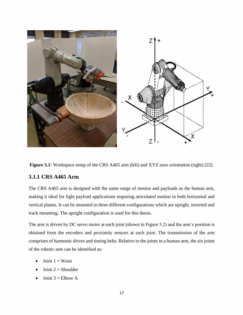
Figure 3.1: Workspace setup of the CRS A465 arm (left) and XYZ axes orientation (right) [22].

3.1.1 CRS A465 Arm

The CRS A465 arm is designed with the same range of motion and payloads as the human arm,

making it ideal for light payload applications requiring articulated motion in both horizontal and

vertical planes. It can be mounted in three different configurations which are upright, inverted and

track mounting. The upright configuration is used for this thesis.

The arm is driven by DC servo motor at each joint (shown in Figure 3.2) and the arm’s position is

obtained from the encoders and proximity sensors at each joint. The transmission of the arm

comprises of harmonic drives and timing belts. Relative to the joints in a human arm, the six joints

of the robotic arm can be identified as:

• Joint 1 = Waist

• Joint 2 = Shoulder

• Joint 3 = Elbow A

18

Figure 3.2: Joint positions of CRS A465 [22].

• Joint 4 = Elbow B

• Joint 5 = Wrist A

• Joint 6 = Wrist B

Performance specifications of the CRS A465 arm are:

• Degrees of Freedom = 6

• Nominal Payload = 2 kg

• Reach (Horizontal) = 711 mm

• Reach (Vertical) = 1041 mm (upwards along Z axis) and 76.2 mm

(downwards below the base level)

• Repeatability = ± 0.05 mm

• Weight = 31 kg

More detailed specifications of the robot arm are given in the User Guide by CRS [23].

As shown in Figure 3.3, the robot has two reference positions: home and ready. The cartesian

coordinates of the home position in the XYZ plane are [-317, 41.8, 836.1] mm. The arm must first

19

Figure 3.3: Home (left) and ready (right) positions of the arm.

be in the home position before teaching locations or running any specific tasks using the teach

pendant or the computer. This allows the arm to synchronize its current position with stored

calibration data. Then the arm is taken to the ready position before executing the desired set of

motions for the task at hand. The cartesian coordinates of the ready position in the XYZ plane are

[406.4, 0, 635] mm. There are two markers on each link of the arm near the joints which are used

to check whether the arm achieved its ready position.

In the ready position, the tool XYZ coordinates align exactly with the world XYZ coordinates and

all the markers on each joint of the arm are lined up.

3.1.2 C500C Controller

The A465 robot uses a CRS C500C as the local controller [24]. Figure 3.4 shows the control

elements of the system: the desktop personal computer (PC), the teach pendant and the C500C

controller box.

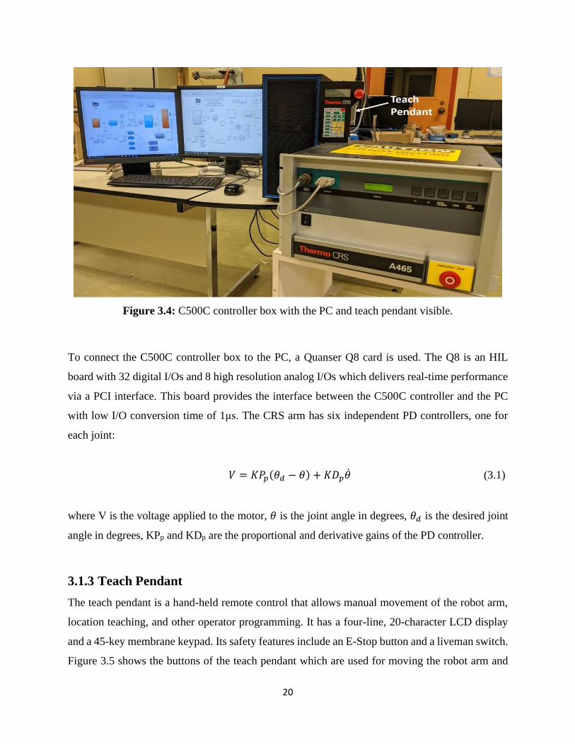
20

Figure 3.4: C500C controller box with the PC and teach pendant visible.

To connect the C500C controller box to the PC, a Quanser Q8 card is used. The Q8 is an HIL

board with 32 digital I/Os and 8 high resolution analog I/Os which delivers real-time performance

via a PCI interface. This board provides the interface between the C500C controller and the PC

with low I/O conversion time of 1μs. The CRS arm has six independent PD controllers, one for

each joint:

𝑉 = 𝐾𝑃𝑝(𝜃𝑑 − 𝜃) + 𝐾𝐷𝑝�̇� (3.1)

where V is the voltage applied to the motor, 𝜃 is the joint angle in degrees, 𝜃𝑑 is the desired joint

angle in degrees, KPp and KDp are the proportional and derivative gains of the PD controller.

3.1.3 Teach Pendant

The teach pendant is a hand-held remote control that allows manual movement of the robot arm,

location teaching, and other operator programming. It has a four-line, 20-character LCD display

and a 45-key membrane keypad. Its safety features include an E-Stop button and a liveman switch.

Figure 3.5 shows the buttons of the teach pendant which are used for moving the robot arm and

21

for gripper movements. The liveman switch is a safety feature whereby teach pendant can be used

to move the arm to home or ready position [25].

Before starting navigation with the teach pendant, there are certain things which must be verified

to conclude that the system is functioning correctly. This is referred to as “commissioning” the

CRS A465 robot [22].

Figure 3.5: Teach pendant [24].

Commissioning involves the following steps that must be performed in order:

1. Checking the arm and controller installation

2. Setting up the teach pendant for commissioning

3. Performing safety checks

4. Checking all E-stops

5. Checking the live-man switch

Liveman Switch

22

Once the system has been commissioned, it is operational and ready to be programmed by the

user.

3.1.4 Computer Software

The two CRS softwares packages originally used to program the arm are:

• Robcomm3 (RAPL-3 Program development environment and interface to C500C)

• POLARA (Laboratory automation software)

It became apparent early in the project that neither could be used as they were no longer compatible

with the PC’s operating system (Win 10). Instead, MATLAB’s Simulink was used to program the

robot in the current PC operating system. In order to interface with Simulink, the CRS A465 robot

requires its own QUARC Simulink library for control of the trajectory and motions. QUARC

ver2.5 was used with MATLAB’s Simulink 2015b for programming the CRS A465 arm in this

application.

The kinematic and dynamic equations derived in Chapter 4 are written in Simulink function blocks

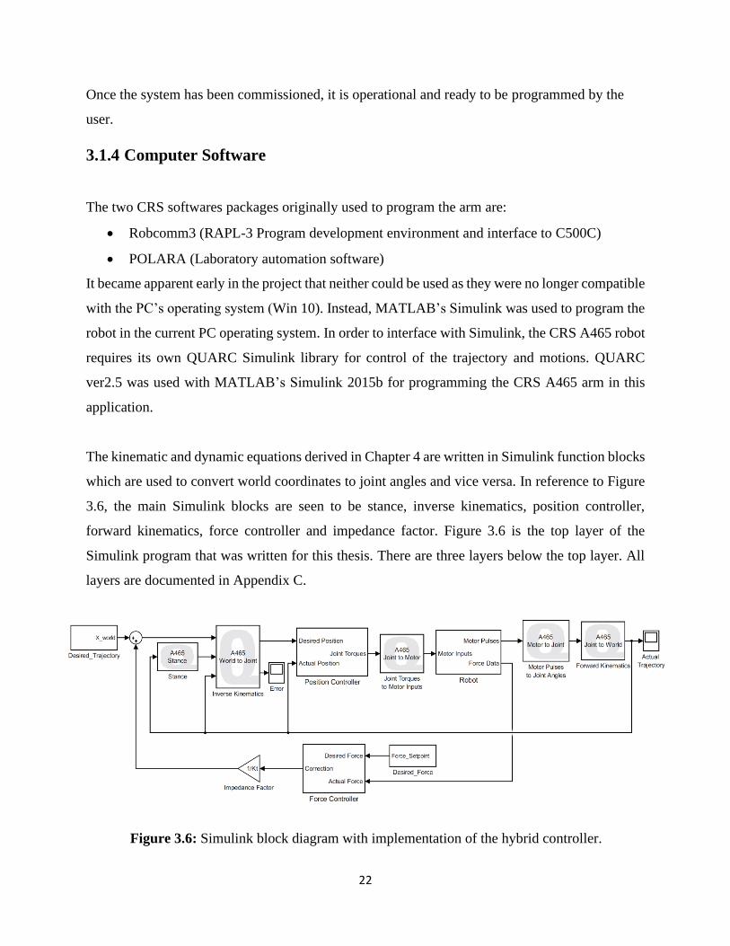
which are used to convert world coordinates to joint angles and vice versa. In reference to Figure

3.6, the main Simulink blocks are seen to be stance, inverse kinematics, position controller,

forward kinematics, force controller and impedance factor. Figure 3.6 is the top layer of the

Simulink program that was written for this thesis. There are three layers below the top layer. All

layers are documented in Appendix C.

Figure 3.6: Simulink block diagram with implementation of the hybrid controller.

23

The Inverse Kinematics block converts the trajectory as given in world coordinates to joint angles.

The Position Controller block tracks the trajectory with feedback from the joint encoders. The

Position Controller block outputs the desired joint torques which are then converted to motor

voltages via the Joint Torques to Motor Inputs block, which are then input to the Robot block. As

outputs from the Robot block, the motor (encoder) pulses are converted back to joint angles using

the Motor Pulses to Joint Angles block, which are then converted to world coordinates using the

Forward Kinematics block. The Force Controller block takes the feedback from the force sensor

and generates the force error which is then added to the desired trajectory after multiplication by

the impedance factor.

3.2 Force Sensor

This force sensor is a compact monolithic load cell manufactured by JR3. It can sense forces and

moments along all three axes of measurement and consequently can measure any three-

dimensional loading. The force sensor is connected to the PC using a National Instruments data

card NI USB-6210. Signals from the sensor are collected in MATLAB using the Quanser toolbox.

For sensor calibration, a Q4 I/O card was used instead of the NI card as the former was easier to

connect without the robot in the loop.

The force sensor was calibrated with static weights before mounting it on the arm. A calibration

matrix is required to give the force output in each axis. The X, Y and Z axes of the force sensor

are shown in the Figure 3.7. The maximum load range of the force sensor in each axis is given in

Appendix A. A 6x6 calibration matrix (as given in Table 3.1) gives all the six values which are

required: Fx, Fy, Fz, Mx, My and Mz (forces and moments in three axes). C1 to C6 are the elements

of the voltage vector output of the force sensor.

24

Table 3.1: Calibration matrix as supplied by JR3 for this particular unit.

C1 C2 C3 C4 C5 C6

Fx 10 −0.267 0.092 −0.606 −0.007 0.663

Fy −0.049 10 0.226 0.056 −0.323 0.011

Fz −0.049 0.078 10 −0.207 0.285 0.418

Mx 0.065 −0.189 −0.056 10 1.397 −0.121

My 0.091 0.003 0.073 1.277 10 −0.111

Mz −0.11 −0.038 0.295 0.106 0.102 10

Figure 3.7: Force sensor axes orientation (JR3).

Figure 3.8: 1kg weight placed on the z axis of the sensor.

To begin, Fz was measured by placing a 1 kg weight on the z axis in the negative direction as

shown in the Figure 3.8. The force offset and gain corrections were obtained by recording the

measured force as the weight was added and then removed (as shown in Figure 3.9). To check the

linearity of the force sensor, different static weights were placed on the z axis of the sensor and

25

the change in force measured (as shown in Figure 3.11). The numerical results are summarized in

Table 3.2.

Figure 3.9: Change in Fz when 1kg weight placed on z axis, with Fx and Fy constant.

In a similar way, static weights were used to calibrate Fx and Fy. Figure 3.10 shows the

arrangement for loading the X axis of the sensor, with a rod inserted through the center of the

sensor and a 1 kg weight suspended under the rod.

Figure 3.10: Arrangement for loading the x axis of the sensor with 1 kg weight.

26

Table 3.2: Correction factors for respective masses in Fz axis.

Static Weight (g) Applied Force (N) Recorded Force (N) Correction Factor

1000 9.81 4.25 0.43

500 4.90 2.25 0.45

400 3.92 1.7 0.43

200 1.96 0.85 0.45

Using the least square method, the equation for the line in Figure 3.10 is:

Fz = 0.432 (Fa) + 0.038 (3.2)

where Fa is the applied force and Fz is the recorded force with correlation Coefficient (r) of

0.999.

Similar results were obtained for X and Y axis. The equations for X and Y axis are given as:

Fx = 0.444 (Fa) + 0.094 (3.3)

Fy = 0.419 (Fa) + 0.010 (3.4)

with correlation Coefficient (r) of 0.996 and 0.998 for X and Y axis respectively. Thus, there is a

strong positive linear relationship between the recorded and applied forces.

Figure 3.11: Plot of recorded force versus applied force.

4.25

2.25

1.7

0.85

y = 0.4321x + 0.038

0

0.5

1

1.5

2

2.5

3

3.5

4

4.5

0 2 4 6 8 10 12

Rec

ord

ed F

orc

e (N

)

Applied Force (N)

27

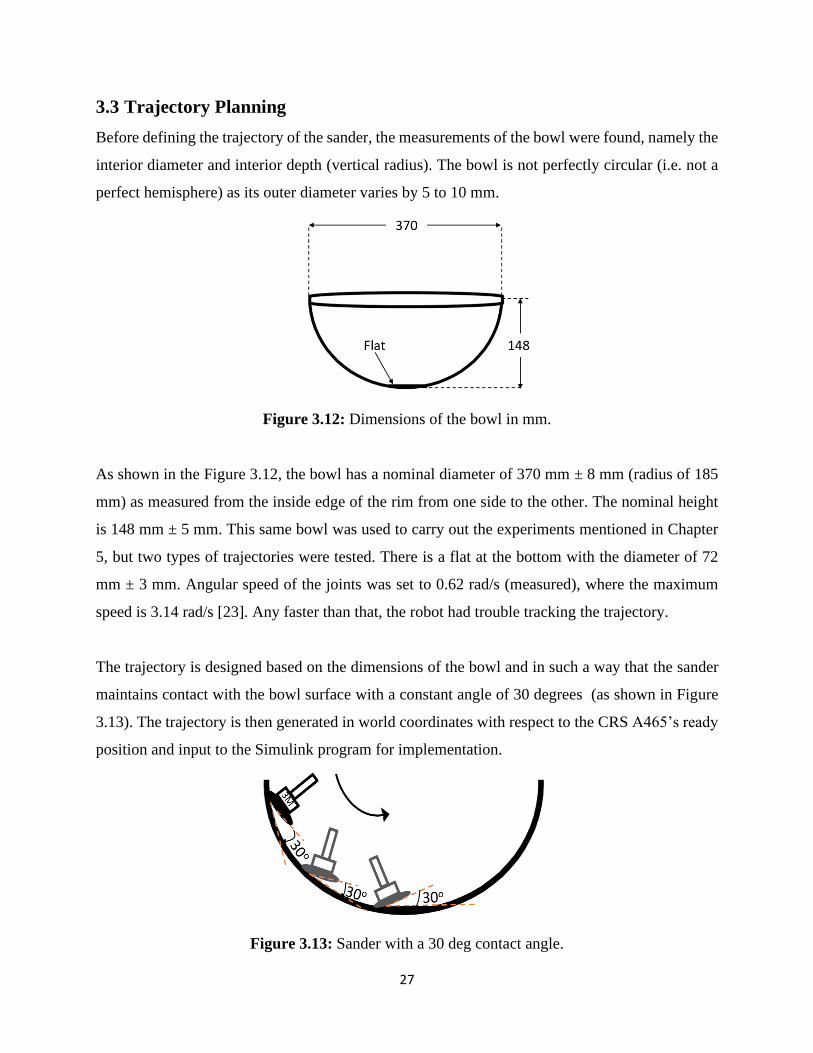
3.3 Trajectory Planning

Before defining the trajectory of the sander, the measurements of the bowl were found, namely the

interior diameter and interior depth (vertical radius). The bowl is not perfectly circular (i.e. not a

perfect hemisphere) as its outer diameter varies by 5 to 10 mm.

Figure 3.12: Dimensions of the bowl in mm.

As shown in the Figure 3.12, the bowl has a nominal diameter of 370 mm ± 8 mm (radius of 185

mm) as measured from the inside edge of the rim from one side to the other. The nominal height

is 148 mm ± 5 mm. This same bowl was used to carry out the experiments mentioned in Chapter

5, but two types of trajectories were tested. There is a flat at the bottom with the diameter of 72

mm ± 3 mm. Angular speed of the joints was set to 0.62 rad/s (measured), where the maximum

speed is 3.14 rad/s [23]. Any faster than that, the robot had trouble tracking the trajectory.

The trajectory is designed based on the dimensions of the bowl and in such a way that the sander

maintains contact with the bowl surface with a constant angle of 30 degrees (as shown in Figure

3.13). The trajectory is then generated in world coordinates with respect to the CRS A465’s ready

position and input to the Simulink program for implementation.

Figure 3.13: Sander with a 30 deg contact angle.

28

3.4 Orbital Sander

The adopted pneumatic orbital sander is manufactured by 3M with a 3-inch head diameter. It is

driven by a portable compressor (details in Appendix A) and runs at a maximum speed of 8000

rpm. The operating pressure of the compressor was maintained at 550 kPa (80 psi) and as sander

starts running, the pressure drops to 345 kPa (50 psi). Its lightweight and low-profile design allows

for sanding in hard-to-reach places. A one-piece shaft balance system minimizes vibration for

greater comfort and smoother results. Initial tests were conducted with a 6-inch Husky palm sander

and 5-inch Bosch random orbit sander (details in Appendix A). They were found to be too heavy

and too large for the application at hand.

The adapter plate (shown in Figure 3.14) for mounting the orbital sander was designed using Solid

Edge and machined from aluminum sheet. The shop drawing for the adapter plate is given in

Appendix A, Figure A.4. The 3M sander is attached to the arm as shown in Figure 3.15.

Figure 3.14: Adapter plate for mounting sander to the wrist.

29

Figure 3.15: Close-up of the end effector, showing mount of the orbital sander and force sensor.

As shown in Figure 3.16, the sander passes along the radial line of the bowl in the XZ plane and

consequently the force acts along the x and z axes of the end effector. The force along the y axis

of the robot is assumed to be zero. The force setpoints along the x and z axes can be determined

from:

Sfx = FN sin Ɵ Sf

z = – FN cos Ɵ (3.5)

where FN is the desired normal force and Ɵ is the contact angle of the sander with the bowl. There

is a negative sign in the equation for Sfz because FN is in the direction of positive x but negative z.

To mimic the human operator, FN is set to 10 N and Ɵ is set to 30 deg. In this case, the resulting

Sfx and Sf

z are 5 N and 8.66 N respectively.

Figure 3.16: Illustration of applied forces by sander in x and z direction.

30

3.5 Vacuum Chuck

The bowl is held in place by a vacuum chuck with a 120 mm diameter as driven by a vacuum

pump as illustrated in Figure 3.17. Three soft rubber rings are placed on the chuck to ensure a tight

seal with the bowl. Specifications of the vacuum pump are given in Appendix A. The vacuum

pressure of the pump while it is running was 62 kPa (9 psi).

Figure 3.17: Vacuum chuck connected to the vacuum pump with bowl sitting on the chuck.

31

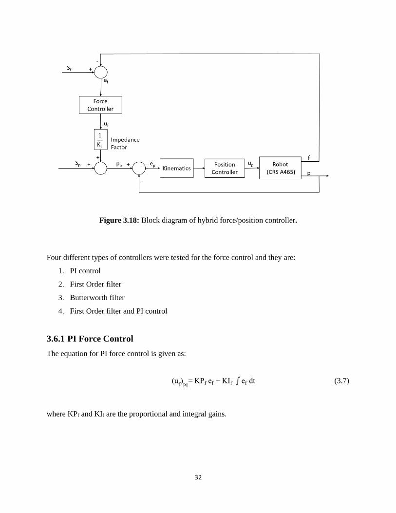
3.6 Controllers

Hybrid force/position impedance control was selected as the controller for this application. As the

name suggests, hybrid force/position control is an approach where different controllers are used

for position and force. In this approach, the force controller feeds the trajectory error into the

position controller through the impedance factor. Changing the impedance factor, changes the

weighting between the force and position control. As recommended by Zeng and Hemami [15],

one approach to hybrid force/position control is to use PI for the force controller and PD for the

position controller.

Thus, a conventional PD controller was used for the position control with control law given as

follows:

ef = Sf – f (3.6a)

po= Sp+

1

𝐾𝑡 (u

f ) (3.6b)

ep= po - p (3.6c)

up= KPp ep + KDp dep

dt (3.6d)

where Sf is the force setpoint, f is the measured force, Sp is the position setpoint, p is the measured

position, ep is error in position, Kt is the impedance factor, KPp and KDp are the proportional and

derivative gains. Recognize that this controller must be implemented three times, one for each of

the three principal axes. The impedance factor given in Equation (3.6b) provides the link between

the force controller and the position controller.

32

Figure 3.18: Block diagram of hybrid force/position controller.

Four different types of controllers were tested for the force control and they are:

1. PI control

2. First Order filter

3. Butterworth filter

4. First Order filter and PI control

3.6.1 PI Force Control

The equation for PI force control is given as:

(uf)PI

= KPf ef + KIf ∫ ef dt (3.7)

where KPf and KIf are the proportional and integral gains.

33

3.6.2 First Order Filter

A First Order filter (FO) can be used to attenuate noise in the force signal before being input to

the position controller. The Cutoff frequency or corner frequency (𝜔𝑐) is the frequency where the

filtered output signal falls to 0.707 (or – 3dB) of the noisy input signal.

The input output relationship for the FO filter is given by:

(uf)FO

= ef

1 + τs (3.8)

where τ is the time constant and 𝜏 =1

𝜔𝑐.

3.6.3 Butterworth Filter

As an example of a higher level filter, a second order low pass Butterworth (BW) filter will be

tested.

The input output relationship for the BW filter is given by:

(uf)BW

=ef

(𝑠

𝜔𝑐)2 + √2 (

𝑠

𝜔𝑐 ) + 1

(3.9)

where 𝜔𝑐 is related to passband edge frequency 𝑓𝑝 by:

𝜔𝑐 =𝑓𝑝

(10−𝐾𝑝10 −1)

12𝑁

(3.10)

where, 𝐾𝑝 is Attenuation at passband frequency 𝑓𝑝 in dB and N is order of the filter.

The BW filter was designed with the “Analog Filter Design” block (as given in Figure A.14) in

Simulink. In which design was selected as BW and filter type as low pass with an order of 2. 𝑓𝑝

for the BW filter was calculated using Equation (3.10) for required 𝜔𝑐.

34

3.6.4 FOPI Force Control

To order to potentially improve the setpoint tracking performance of the force controller, a PI

controller was added to the FO filter, with the FO/PI control law given as:

(uf)FOPI

= KPf 𝑒𝑓

1 + 𝜏𝑠 + KIf ∫

𝑒𝑓

1 + 𝜏𝑠 dt (3.11)

This completes the documentation of the four force controllers and the PD position controller.

3.7 Summary

This chapter documented the test apparatus developed for this application. The apparatus

consists of four main components:

• 6 - axis Articulated robot

• 3 - axis force sensor

• Orbital sander

• Vacuum chuck

Hybrid force/position impedance control was selected to control both force and position. A PD

controller will be used for position control and four controller configurations will be tested for

force control:

• First Order filter

• Butterworth filter

• PI control

• FO filter with PI control

Adjustment to the impedance factor will determine the relative weighting between the position

and force controllers.

35

CHAPTER 4

KINEMATICS AND DYNAMICS

An accurate kinematic and dynamic model of a robotic arm is needed in order generate the

individual motor motions required for the end effector to follow the desired point by point

trajectory while maintaining the desired angle relative to the workpiece. This chapter sets out to

derive and document the model for the CRS A465 arm. Before formulating the kinematic

equations, the DH parameters are obtained by describing the arm mathematically. The

transformation matrices are derived from the DH parameters to describe the relationship between

paired joint frames. Using the transformation matrices, the forward and inverse kinematic

equations are formulated to obtain the relationship between the end effector position coordinates

and the joint angles. Next, the differential kinematics are derived to give the relationship between

the joint velocities and corresponding end-effector linear and angular velocity. In order to do this,

the Jacobian matrix is computed for all six revolute joints. Finally, the joint equations are

formulated to give the relationship between mass and inertia properties, motion and the associated

forces and torques. The dynamic equations are needed for force estimation, trajectory design and

its optimization.

4.1 DH Parameters

To determine the equations that provide the basis for the forward and inverse kinematics of the

robot, it is necessary to describe the arm mathematically. The conventions of Denavit-Hartenberg

(DH) will be used (Tsai et al, [12]).

In determining the DH parameters, the first step is to produce a diagram, which completely

describes the mechanism in question. A DH diagram is typically used for this purpose, where each

joint gives rise to a new frame of reference. For the CRS A465 arm, the DH diagram is given as

Figure 4.1.

36

Each frame in the DH diagram can be described by parameters including link length (ai), link

twist (αi), joint angle (Θi) and joint offset (di) for each joint where to be precise for joints 1 to 6:

• αi = the angle between Zi-1 to Zi measured about Xi;

• ai = the distance from Zi-1 to Zi measured along Xi;

• di = the distance from Xi-1 to Xi measured along Zi;

• Θi = the angle between Xi-1 to Xi measured about Zi;

There is some degree of ambiguity as to the way this table was obtained. For example, Frame 0 is

positioned at the same position as Frame 1: at the top of the base column. This was done so as to

simplify the calculations; however, it would be equally correct to include a value of 330.2 mm (the

height of the base column) in cell d1. This change would, of course, reflect itself in slightly altered

equations, however the result at the end would be the same. Similarly, it would be correct to

describe the wrist by assigning values of 𝜋/2, -𝜋/2, and 𝜋/2 to 𝛼3, 𝛼4, and 𝛼5.)

Based on Figure 4.1, the DH parameters of the CRS A465 arm can be obtained. They are

summarized in Table 4.1:

Table 4.1: DH parameters for all six joints of CRS A465 arm.

i Joint αi ai di Θi

1 Waist 𝜋/2 0 0 Θ1

2 Shoulder 0 304.8 mm 0 Θ2

3 Elbow A -𝜋/2 0 0 Θ3

4 Elbow B 𝜋/2 0 330.2 mm Θ4

5 Wrist A -𝜋/2 0 0 Θ5

6 Wrist B 0 0 0 Θ6

37

Figure 4.1: Denavit-Hartenberg (DH) diagram of the CRS A465 arm [25].

4.1.1 Transformation Matrices

The purpose of the forward and inverse kinematics equations is to allow one to find a means of

describing the position and orientation of the end effector given the joint angles (and vice versa).

Position and orientation, relative to a given base frame are often described by means of a 4x4

transformation matrix. For example, the following matrix describes the position and orientation

when moving from Frame a to Frame b.

𝑇𝑏𝑎 = [

𝑟11 𝑟12 𝑟13 𝑝𝑥

𝑟21 𝑟22 𝑟23 𝑝𝑦

𝑟31 𝑟32 𝑟33 𝑝𝑧

0 0 0 1

] (4.1)

The terms 𝑟11 to 𝑟33 describe the change in orientation, while the terms 𝑝𝑥, 𝑝𝑦 and 𝑝𝑧 describe

the change in position.

38

Now, given some Frame i as described by four DH parameters, it is possible to derive the

transformation matrix that describes the relationship between Frame i-1 and Frame i. The general

form of doing so is as follows:

Tii−1 = [

cos θi −sin θi 0 ai−1

sin θi cos αi−1 cos θi cos αi−1 −sin αi−1 −sin αi−1 di

sin θi sin αi−1 cos θi sin αi−1 cos αi−1 cos αi−1 di

0 0 0 1

] (4.2)

In general, transformation matrices can be designated as 𝑇𝑦𝑥 if they describe the transformation

from frame x to frame y.

From this template, together with the DH parameters given in Table 4.1, it is possible to derive

the transformation matrices between each of the frames of the arm. They are as follows:

𝑇10 = [

𝑐1 −𝑠1 0 0𝑠1 𝑐1 0 00 0 1 𝑑1

0 0 0 1

] 𝑇21 = [

𝑐2 −𝑠2 0 00 0 −1 0𝑠2 𝑐2 0 00 0 0 1

]

𝑇32 = [

𝑐3 −𝑠3 0 𝐴2

𝑠3 𝑐3 0 00 0 1 00 0 0 1

] 𝑇43 = [

𝑐4 −𝑠4 0 00 0 −1 𝐷4

−𝑠4 −𝑐4 0 00 0 0 1

]

𝑇54 = [

𝑐5 −𝑠5 0 00 0 −1 0𝑠5 𝑐5 0 00 0 0 1

] 𝑇65 = [

𝑐6 −𝑠6 0 00 0 −1 0

−𝑠6 −𝑐6 0 00 0 0 1

] (4.3)

where c1 cos 𝜃1, s1 sin 𝜃1, s23 sin (𝜃2 + 𝜃3), and so on. However, to create the kinematics

equations, individual transformation matrices is the first step. A transformation matrix is still

required that completely describes the position and orientation of the tool tip with respect to the

39

base of the robot. As there are six joints in the CRS A465 arm, and hence six intermediate frames,

the total base-to-tip transformation matrix can be designated as 𝑇 60 . Fortunately, this matrix follows

easily from the six individual matrices as follows:

𝑇60 = 𝑇1

0 𝑇21 𝑇3

2 𝑇 43 𝑇5

4 𝑇65 (4.4)

4.2 Forward Kinematics

In order to manipulate an object, one must be able to specify the position and orientation of the

end-effector with respect to a reference frame. Only joint variables are evaluated in most

manipulators. Typically, forward kinematics equations are used to compute the world position

coordinates and orientation of the tool tip for each of the six joint angles of the arm by way of a

transformation matrix.

𝑇60 = [

𝑟11 𝑟12 𝑟13 𝑝𝑥

𝑟21 𝑟22 𝑟23 𝑝𝑦

𝑟31 𝑟32 𝑟33 𝑝𝑧

0 0 0 1

] (4.5)

where 𝑟11 to 𝑟33 describe the change in orientation, and the terms 𝑝𝑥, 𝑝𝑦 and 𝑝𝑧 describe the

change in position.

The components of the transformation matrix can be broken down by the normal vector (n), slide

vector (s), approach vector (a) and translation vector (p) is given as:

𝑇60 = [𝑛6

0 𝑠60 𝑎6

0 𝑝60

0 0 0 1] (4.6)

By multiplying together, the matrices given in Equation (4.3) in the correct order, the desired 𝑇60

transformation matrix can be derived in terms of the given joint angles. Specifically, the following

vectors can be formulated:

40

n60 = [

r11

r21

r31

] = [

c1 (c23 (c4c5c6 − s4s6) − s23s5c6) – s1 (s4c5c6 + c4s6)

s1 (c23 (c4c5c6 − s4s6) − s23s5c6) + c4 (s4c5c6 + c4s6)s23 (c4c5s6 − s4c6) + c23s5s6

] (4.7)

s60 = [

r12

r22

r32

] = [

c1 (−c23 (c4c5s6 + s4c6) + s23s5s6) – s1 (−s4c5s6 + c4c6)

s1 (−c23 (c4c5s6 + s4c6) + s23s5s6) + c1 (−s4c5s6 + c4c6)

−s23 (c4c5s6 + s4c6) − c23s5s6

] (4.8)

a60 = [

r13

r23

r33

] = [−c1 (c23c4s5 + s23c5) + s1 (s4s5)

−s1 (c23c4s5 + s23c5) − c1 (s4s5)−s23c4s5 + c23c5

] (4.9)

p60 = [

px

py

pz

] = [

c1 (−D4s23 + A2c2)s1 (−D4s23 + A2c2)D4c23 + A2s2 + d1

] (4.10)

It should be noted that A2 and D4 are the lengths of links 2 and 3 respectively with d1 = 0 (see

Figure 4.1). Furthermore, in case of discrepancy between these equations and those found in the

c-code, the latter shall be considered correct. It now becomes a straightforward matter to obtain

the elements of the equations to determine the elements of the 𝑇60

transformation matrix. In fact,

because one knows that the three column vectors of orientation are orthogonal unit vectors, one

need only calculate two of the three vectors and determine the last vector by taking their cross

product.

The CRS A465 Joint to World block inside the Forward Kinematics block (given in Figure C.19)

converts the joint angles to cartesian coordinates and the Stance block gives the arm’s

configuration (orientation) to reach the required end point position.

4.3 Inverse Kinematics

As the name would suggest, inverse kinematics does the opposite of the forward kinematics. That

is, given the world coordinate position and orientation of a robot end effector, the positions of each

of the robot joints will be returned. However, a given set of joint angles can only be attained by

41

one world position and orientation, the converse is not true. There may be as many as eight valid

joint solutions for a manipulator such as the CRS A465 arm, for any specified position and

orientation. The inverse kinematics model will solve each of the eight alternatives and then pass

the outcomes to a selection routine that will determine the best solution based on the required

current stance and the previous arm position.

For each of the following solutions, it is assumed the 𝑇60 transformation matrix is known (because

one is operating from a known position and orientation). This is used along with some intermediate

matrices that can be calculated from the list of joint matrices provided in Equation 4.3.

Joint 1 solution

With the following transformation matrix as the starting point:

𝑇60 = 𝑇1

0 𝑇61

it follows that

[ 𝑇10 ]−1 𝑇6

0 = 𝑇61

or more simply

𝑇01 𝑇 = 𝑇6

160 (4.11)

If the Element (2,4) is extracted from Equation 4.11, the following is obtained

−𝑠1𝑝𝑥 + 𝑐1𝑝𝑦 = 0

and hence the resulting forward solution for the angle of Joint 1 is:

𝛩1𝐹 = 𝑎𝑡𝑎𝑛2 (𝑝𝑦, 𝑝𝑥) (4.12)

42

As determined by the signs of px and py, the function atan2 has a range of [-π, + π] whereas the

function atan has a range of [-π /2, + π /2].)

Finally, given that the arm can reach backwards, the resulting backward solution is:

Θ1𝐵 = Θ1𝑎 + π (4.13)

Joint 3 Solution

The same matrix equation 𝑇01 𝑇6

0 = 𝑇61 is used to solve for Joint 3. If the Element (1,4) is

extracted from Equation (4.11), the following can be obtained

𝑐1𝑝𝑥 + 𝑠1𝑝𝑦 = −𝑠23𝐷4 + 𝐴2𝑐2

Also, for Element(3,4) from Equation (4.11),

𝑝𝑧 = 𝑐23𝐷4 + 𝑠2𝐴2

and for Element (2,4)

−𝑠1𝑝𝑥 + 𝑐1𝑝𝑦 = 0

Combining all three equations:

(𝑐1𝑝 𝑥 + 𝑠1𝑝𝑦 )2 + 𝑝𝑧2 = (𝐷4

2 + 𝐴22) + 2𝐷4𝐴2(𝑐23𝑠2 − 𝑠23𝑐2)

which, with some substitutions, it can be rewritten as:

(𝑏𝑎𝑠𝑒𝑝𝑙𝑎𝑛𝑒_𝑑𝑖𝑠𝑡)2 + 𝑝𝑧2 = 𝑙𝑖𝑛𝑘𝑣𝑎𝑟1 − 2𝐷4𝐴2𝑠3

where, 𝑙𝑖𝑛𝑘𝑣𝑎𝑟1 = (𝐷42 + 𝐴2

2) and 𝑏𝑎𝑠𝑒𝑝𝑙𝑎𝑛𝑒_𝑑𝑖𝑠𝑡 = 𝑐1𝑝 𝑥 + 𝑠1𝑝𝑦. Thus, this can be

rewritten as:

2𝐷4𝐴2𝑠3 = 𝑡𝑚𝑝1

43

Using the formula

𝑐3 = ±√1 − 𝑠32

The following equation can be derived by substituting 𝑐3 as tmp1:

2𝐷4𝐴2𝑐3 = ±√4𝐷42𝐴2

2 − 𝑡𝑚𝑝12

Therefore, the angle of Joint 3 can be obtained from:

𝛩 3 = 𝑎𝑡𝑎𝑛2(𝑡𝑚𝑝1, ±√4𝐷42𝐴2

2 − 𝑡𝑚𝑝12) (4.14)

Equation 4.14 has two possible solutions, corresponding to the two solutions of the square root. It

is not computationally efficient to calculate the atan2 function more often than necessary, and so

the equation is rewritten as:

Θ3BUFD = π /2 + atan2(−√4D42A2

2 − tmp12, tmp1) (4.15)

Θ3FUBD = π /2 − atan2 (−√4𝐷42𝐴2

2 − 𝑡𝑚𝑝12, tmp1) (4.16)

Which allows us to find both solutions while computing the atan2 only once.

Note that BUFD refers to the “backward-up/forward-down” elbow configuration, while FUBD

refers to the “forward-up/backward-down” configuration.

Joint 2 Solution

To solve for joint 2, some of the previously established transformation matrices can be

rearranged to arrive at:

𝑇03 𝑇 = 𝑇6

360 (4.17)

From Equation (4.17), the elements of 𝑇63 can be extracted:

44

For Element (1,4)

𝑐1𝑐23𝑝𝑥 + 𝑠1𝑐23𝑝𝑦 + 𝑠23𝑝𝑧 (−𝐴2𝑐3) = 0

For Element (2, 4)

−𝑐1𝑠23𝑝𝑥 − 𝑠1𝑠23𝑝𝑦 + 𝑐23𝑝𝑧 (𝐴2𝑠3) = 0

For Element (1, 4)

𝑐23 (𝑐1𝑝𝑥 + 𝑠1𝑝𝑦 ) + 𝑠23𝑝𝑧 –𝐴2𝑐3 = 0

and for Element (2, 4)

𝑠23 (−𝑐1𝑝𝑥 − 𝑠1𝑝𝑦) + 𝑐23𝑝𝑧 + 𝐴2𝑠3 = 𝐷4

which can be combined to solve for s23 and c23:

𝑠23 = A2c3p𝑧 − ((D4 − A2s3) ∗ baseplane_dist)

𝑡ℎ𝑟𝑒𝑒𝑠𝑝𝑎𝑐𝑒_𝑑𝑖𝑠𝑡_𝑠𝑞𝑟

𝑐23 = (D4 − A2s3)p𝑧 − (A2c3 ∗ baseplane_dist)

𝑡ℎ𝑟𝑒𝑒𝑠𝑝𝑎𝑐𝑒_𝑑𝑖𝑠𝑡_𝑠𝑞𝑟

where, 𝑡ℎ𝑟𝑒𝑒𝑠𝑝𝑎𝑐𝑒_𝑑𝑖𝑠𝑡_𝑠𝑞𝑟 = (𝑐1𝑝 𝑥 + 𝑠1𝑝𝑦)2 + p𝑧2

Thus, the joint angle for Joint 2 can be obtained from:

Θ2 = atan2(s23, c23) − Θ3 (4.18)

Joint 4 Solution

For this joint, the same matrix equation is used as in the case for Joint 2. From Equation (4.17),

the elements of 𝑇63 are extracted:

45

For Element (1,3)

𝑐1𝑐23𝑟13 + 𝑠1𝑐23𝑟23 + 𝑠23𝑟33 = −𝑐4𝑐5

and for Element (3,3)

𝑠1𝑟13 – 𝑐1𝑟23 = 𝑠4𝑠5

Note that “wrist-flipped” refers to the Joint 4 rotated by 180 deg from ready position. Solving

these for s4 and c4, the wrist-flipped solution for Joint 4 was derived as:

Θ4F = atan2[ (−s1r13 + c1r23), (c1c23r13 + s1c23r23 + s23r33) ] (4.19)

as well as the secondary, wrist-not-flipped solution for Joint 4 is:

Θ4N = Θ4F + π (4.20)

Joint 5 Solution

Beginning with the matrix equation

𝑇04 𝑇 = 𝑇6

460 (4.21)

The elements of 𝑇64 can be extracted from the Equation (4.21) as follows:

For Element (1,3)

𝑟13(−𝑠1𝑠4 + 𝑐1𝑐23𝑐4) + 𝑐23(𝑐1𝑠4 + 𝑠1𝑐23𝑐4) + 𝑟33(𝑠23𝑐4) = −𝑠5

and for Element (3,3)

−c1s23r13 – s1s23r23 + 𝑐23r33 = 𝑐5

to arrive at the wrist-not-flipped solution for Joint 5 as:

Θ5N = 𝑎𝑡𝑎𝑛2( 𝑠5, 𝑐5 ) (4.22)

46

and the resulting wrist-flipped solution for Joint 5 is:

Θ5F = − Θ5N (4.23)

Joint 6 Solution

Using the matrix equation

𝑇05 𝑇 = 𝑇6

560 (4.24)

The elements of 𝑇65 are extracted from the Equation (4.24) to arrive at:

For Element (1,2)

𝑟12(−𝑐5𝑠1𝑠4 + 𝑐5𝑐1𝑐23𝑐4 − 𝑠5𝑐1𝑠23) +

𝑟22(𝑐5𝑐1𝑠4 + 𝑐5𝑠1𝑐23𝑐4 − 𝑠5𝑠1𝑠23) +

𝑟32(𝑐5𝑠23𝑐4 + 𝑠5𝑐23) = −𝑠6

For Element (3,2)

𝑟12(−𝑐1𝑐23𝑠4 − 𝑠1𝑐4) + 𝑟22(−𝑠1𝑐23𝑠4 + 𝑐1𝑐4) – 𝑠23𝑠4𝑟32 = 𝑐6

which can be used directly to produce the wrist-not-flipped solution for Joint 6 as:

Θ6N = 𝑎𝑡𝑎𝑛2( 𝑠6, 𝑐6 ) (4.25)

and the resulting wrist-flipped solution for Joint 6 is:

Θ6F = Θ6N + π (4.26)

A465 Stance is the block used in Simulink (refer to Figure C.3) to determine the joint configuration

of the arm for a desired position. This block calculates stance from the joint angle feedback. An

auto stance configuration [-1 -1 -1] can be used in situations where the controller is allowed to

select the best stance to reach desired position automatically.

47

4.4 Differential Kinematics

In this section, differential kinematics are used to compute the “Jacobian” matrix which is used to

map the joint velocities to the respective end-effector’s linear and angular velocities. The

conversion of joint velocity to end-effector angular/linear velocity can be expressed as (Croft et al

[14]):

[𝑣𝜔

] = 𝐽�̇� (4.27)

where J is the Jacobian matrix, 𝑣 is the linear velocity, 𝜔 is the angular velocity and �̇� is the joint

velocity.

The Jacobian for a revolute joint is given as:

J𝑖 = [𝑧𝑖−1

0 × (𝑝𝑛0 − 𝑝𝑖−1

0 )

𝑧𝑖−10 ]

For the CRS A465 arm, the six revolute joints must be considered first, so the general matrix for

the Jacobian looks like the following

J = [𝑧0

0 × (𝑝60 − 𝑝0

0) 𝑧10 × (𝑝6

0 − 𝑝10) 𝑧2

0 × (𝑝60 − 𝑝2

0) . . . 𝑧50 × (𝑝6

0 − 𝑝50)

𝑧00 𝑧1

0 𝑧20 . . . 𝑧5

0 ]

(4.28)

where 𝑧20 is the approach of the 2nd frame in Frame 0 (same as term ‘a’ in forward kinematics)

and 𝑝60 is the position vector of the 6th frame in Frame 0. Using the values of these parameters, as

computed in Section 4.2 (Forward Kinematics), each term in the above Jacobian computes out to

be:

𝑝00 = 𝑝1

0 = [00𝑑1

] ; 𝑝20 = [

A2c1c2

A2s1c2

s2𝐴2

]

48

𝑝30 = 𝑝4

0 = 𝑝50 = [

c1 (−D4s23 + A2c2)

s1 (−D4s23 + A2c2)D4c23 + A2s2 + 𝑑1

]

𝑧00 × (𝑝6

0 − 𝑝00) = [

001] × [

c1 (−D4s23 + A2c2)s1 (−D4s23 + A2c2)

D4c23 + A2s2

] = [−s1 (−D4s23 + A2c2)−c1 (−D4s23 + A2c2)

0

]

𝑧10 × (𝑝6

0 − 𝑝10) = [

s1

−c1

0] × [

c1 (−D4s23 + A2c2)s1 (−D4s23 + A2c2)

D4c23 + A2s2

] = [

−c1 (D4c23 + A2s2)s1 (D4c23 + A2s2)−D4s23 + A2c2

]

𝑧20 × (𝑝6

0 − 𝑝20) = [

s1

−c1

0] × [

c1 (−D4s23)s1 (−D4s23)

D4c23

] = [−D4c1c23

D4s1c23

−D4s23

]

𝑧30 × (𝑝6

0 − 𝑝30) = [

c1s23

s1s23

−c23

] × [000] = [

000]

𝑧40 × (𝑝6

0 − 𝑝40) = [

c1s4s23 + s1s4

s1s4c23 + c1s4

s23s4

] × [000] = [

000]

𝑧50 × (𝑝6

0 − 𝑝50) = [

−c1 (c23c4s5 + s23c5) + s1 (s4s5)

−s1 (c23c4s5 + s23c5) − c1 (s4s5)−s23c4s5 + c23c5

] × [000] = [

000]

Adding all the above elements to Equation (4.28), one gets the Jacobian matrix. Finally, the

angular and linear velocities are computed to be

v = [

𝑣1

𝑣2

𝑣3

] = [

−s1 (−D4s23 + A2c2)�̇�1 − c1 (D4c23 + A2s2)�̇�2 − D4c1c23�̇�3

−c1 (−D4s23 + A2c2)�̇�1 + s1 (D4c23 + A2s2)�̇�2 + D4s1c23�̇�3

(−D4s23 + A2c2)�̇�2 −D4s23�̇�3

] (4.29)

49

𝜔 = [

𝜔1

𝜔2

𝜔3

]

= [

s1�̇�2 + s1�̇�3 + c1s23�̇�4 + (c1s4s23 + s1s4)�̇�5 + (−c1 (c23c4s5 + s23c5) + s1 (s4s5))�̇�6

−c1�̇�2−c1�̇�3 + s1s23�̇�4 + (s1s4c23 + c1s4)�̇�5 + (−s1 (c23c4s5 + s23c5) − c1 (s4s5))�̇�6

�̇�1 − c23�̇�4 + s23s4�̇�5 + (−s23c4s5 + c23c5)�̇�6

]

(4.30)

4.5 Robot Dynamics

This section gives the dynamic equations derived for the CRS A465 arm. The generic model for

robot dynamics can be given as [13]:

(𝐷(𝑞) +𝐼𝑚

𝑟2) �̈� + (𝐶(𝑞, �̇�) + 𝐵)�̇� + 𝐺(𝑞) + 𝐹𝑠(�̇�) =𝐾𝑉

𝑟= 𝜏 − 𝐽𝑇𝐹𝑒𝑥𝑡 (4.31)

where D(q) is the manipulator mass matrix, Im is the motors inertia matrix, C(q, q̇) is the Coriolis

and centrifugal matrix, B is the viscous friction matrix, G(q) is the gravitational vector, 𝐹𝑠(�̇�) is

the Coulomb friction matrix, r is the gear ratio, 𝑉 = [𝑉1 𝑉2 𝑉3]𝑇 is the commanded voltage vector,

K is a scalar conversion from commanded voltage to motor torque, 𝑞 = [𝑞1 𝑞2 𝑞3]𝑇 is the

manipulator joint position, 𝜏 is the total joint torque, and 𝐹𝑒𝑥𝑡 is the force applied by the end-

effector (i.e. the sander). The commanded voltage signal acquired after the internal joint position

PD controller of the robot as given in Equation (3.1). Since one does not have access to the

amplifier gains for the voltage to motor torques, K is an unknown. Thus, all parameters described

in this section will be given as a function of K.

4.5.1 Lagrange

A Lagrangian approach can be used to find the dynamic equations of the arm. The generic

Lagrangian for a manipulator is written as L = 𝐾𝐸 − 𝑃𝐸, where KE and PE represents the kinetic

and potential energies respectively and are defined as:

50

𝐾𝐸 = ∑1

2

6𝑖=1 [𝑚𝑖𝑣𝑐𝑖

𝑇 𝑣𝑐𝑖 + (𝜔𝑖𝑖)𝑇𝐼𝑖𝜔𝑖

𝑖] (4.32)

𝑃𝐸 = ∑ −𝑚𝑖𝑔𝑇𝑃𝑐𝑖

6𝑖=1 (4.33)

where i is the link number, 𝑚𝑖 is mass of the link I, 𝑣𝑐𝑖 = 𝑃𝑖−10 + (𝜔𝑖

0) × 𝑟𝑖−1,𝑐𝑖

0 is the linear

velocity of the center of mass of link I, (𝜔𝑖𝑖) = (𝑅𝑖

0)𝑇𝜔𝑖0 is the angular velocity of link I, 𝐼𝑖 is the

inertia tensor of link I, g = [0 0 9.80574]T is the gravitational acceleration vector and 𝑃𝑐𝑖 is the

position of the center of mass of link i. To reduce the complexity in computing the dynamics, only

the principal moment of inertia is taken for each link. Hence, 𝐼𝑖 was assumed as:

𝐼𝑖 = [

𝐼𝑖𝑥𝑥 0 00 𝐼𝑖𝑦𝑦 0

0 0 𝐼𝑖𝑧𝑧 ] (4.34)

The distances described by the vector 𝑟𝑖−1,𝑐𝑖

0 between the center of mass of link i and the center

of Frame {i-1} are defined as:

𝑟0,𝑐1

0 = 𝑅10[0 𝑙𝑐1 0]𝑇; 𝑟1,𝑐2

0 = 𝑅20[𝑙𝑐2 0 0]𝑇; 𝑟2,𝑐3

0 = 𝑅30[0 0 𝑙𝑐3]

𝑇;

𝑟3,𝑐4

0 = 𝑅30[0 𝑙𝑐4 0]𝑇; 𝑟4,𝑐5

0 = 𝑅30[0 0 𝑙𝑐5]

𝑇; 𝑟5,𝑐6

0 = 𝑅30[𝑙𝑐6 0 0]𝑇 (4.35)

where the rotation matrix 𝑅𝑖0 are obtained from the transformation matrices presented in Section

4.1 and the angular velocities 𝜔𝑖0 for the links with respect to frame zero are obtained from:

𝜔10 = [

00𝑞1̇

]

𝜔20 = [

sin (𝑞1)𝑞2̇

−cos (𝑞1)𝑞2̇

𝑞1̇

]

51

𝜔30 = [

sin (𝑞1)(𝑞2̇ + 𝑞3̇)

−cos (𝑞1)(𝑞2̇ + 𝑞3̇)𝑞1̇

]

𝜔40 = [

sin(𝑞1) (𝑞2̇ + 𝑞3̇) + cos(𝑞1) sin(𝑞2 + 𝑞3) 𝑞4̇

−cos(𝑞1) (𝑞2̇ + 𝑞3̇) + sin(𝑞1) sin(𝑞2 + 𝑞3) 𝑞4̇

𝑞1̇ − cos(𝑞2 + 𝑞3) 𝑞4̇

]

𝜔50

= [

sin(𝑞1) (𝑞2̇ + 𝑞3̇) + cos(𝑞1) sin(𝑞2 + 𝑞3) 𝑞4̇ + (cos(𝑞1) sin(𝑞4) sin(𝑞2 + 𝑞3) + sin(𝑞1) sin(𝑞4))𝑞5̇

−cos(𝑞1) (𝑞2̇ + 𝑞3̇) + sin(𝑞1) sin(𝑞2 + 𝑞3) 𝑞4̇ + (sin(𝑞1) sin(𝑞4) sin(𝑞2 + 𝑞3) + cos(𝑞1) sin(𝑞4))𝑞5̇

𝑞1̇ − cos(𝑞2 + 𝑞3) 𝑞4̇ + sin(𝑞2 + 𝑞3) sin(𝑞4) 𝑞5̇

]

𝜔60 = [

𝜔60(1)

𝜔60(2)

𝜔60(3)

] (4.36)

where

𝜔60(1) = cos(𝑞1) (sin(𝑞2 + 𝑞3) 𝑞4 + cos(𝑞2 + 𝑞3) cos(𝑞4) sin(𝑞5) + sin(𝑞2 + 𝑞3) cos(𝑞5))

+ (cos(𝑞1) sin(𝑞4) sin(𝑞2 + 𝑞3) + sin(𝑞1) sin(𝑞4))𝑞5̇ + sin(𝑞1) ((𝑞2̇ + 𝑞3̇)

+ (sin(𝑞4) sin(𝑞5)))𝑞6̇

𝜔60(2) = sin(𝑞1) (sin(𝑞2 + 𝑞3) 𝑞4 − cos(𝑞2 + 𝑞3) cos(𝑞4) sin(𝑞5) − sin(𝑞2 + 𝑞3) cos(𝑞5))

+ (sin(𝑞1) sin(𝑞4) sin(𝑞2 + 𝑞3) + cos(𝑞1) sin(𝑞4))𝑞5̇ − cos(𝑞1)((𝑞2̇ + 𝑞3̇)

+ (sin(𝑞4) sin(𝑞5)))𝑞6̇

𝜔60(3) = 𝑞1̇ − cos(𝑞2 + 𝑞3) 𝑞4̇ + sin(𝑞2 + 𝑞3) sin(𝑞4) 𝑞5̇ + (−sin(𝑞2 + 𝑞3) cos(𝑞4) sin(𝑞5)

+ cos(𝑞2 + 𝑞3) cos(𝑞5))𝑞6̇

4.5.2 Mass and Inertia Terms

The manipulator mass matrix D(q) is obtained using the kinetic energy (KE) equation since it is

known that

𝐾𝐸 =1

2�̇�𝑇𝐷(𝑞)�̇� (4.37)

52

Therefore, after computing KE with the forward kinematics equations, D(q) is extracted by

factoring the joint velocities. The resulting matrix is:

𝐷(𝑞) =

[ 𝑑11 𝑑12 𝑑13 𝑑14 𝑑15 𝑑16

𝑑21 𝑑22 𝑑23 𝑑24 𝑑25 𝑑26

𝑑31 𝑑32 𝑑33 𝑑34 𝑑35 𝑑36

𝑑41 𝑑42 𝑑43 𝑑44 𝑑45 𝑑46

𝑑51 𝑑52 𝑑53 𝑑54 𝑑55 𝑑56

𝑑61 𝑑62 𝑑63 𝑑64 𝑑65 𝑑66]

=

[ 𝑑11 0 0 0 0 00 𝑑22 𝑑23 𝑑24 𝑑25 𝑑26

0 𝑑32 𝑑33 𝑑34 𝑑35 𝑑36

0 𝑑42 𝑑43 𝑑44 𝑑45 𝑑46

0 𝑑52 𝑑53 𝑑54 𝑑55 𝑑56

0 𝑑62 𝑑63 𝑑64 𝑑65 𝑑66]

(4.38)

The non-zero matrix elements in the Equation (4.38) are given in Appendix B. The mass matrix is

symmetric in nature. Thus, the terms 𝑑𝑖𝑗 = 𝑑𝑗𝑖 where i and j are row and column of the mass

matrix. Regarding the inertia of the motors, it can be defined as the matrix 𝐼𝑚:

𝐼𝑚 =

[ 𝐼𝑚1 0 0 0 0 00 𝐼𝑚2 0 0 0 00 0 𝐼𝑚3 0 0 00 0 0 𝐼𝑚4 0 00 0 0 0 𝐼𝑚5 00 0 0 0 0 𝐼𝑚6]

(4.39)

4.5.3 Coriolis and Centrifugal Terms

The matrix 𝐶(𝑞, �̇�)in Christoffel form containing the coriolis and centrifugal terms is defined as:

𝐶(𝑞, �̇�) =

[ 𝑐11 𝑐12 𝑐13 𝑐14 𝑐15 𝑐16

𝑐21 𝑐22 𝑐23 𝑐24 𝑐25 𝑐26

𝑐31 𝑐32 𝑐33 𝑐34 𝑐35 𝑐36

𝑐41 𝑐42 𝑐43 𝑐44 𝑐45 𝑐46

𝑐51 𝑐52 𝑐53 𝑐54 𝑐55 𝑐56

𝑐61 𝑐62 𝑐63 𝑐64 𝑐65 𝑐66]

(4.40)

can be obtained using the manipulator mass matrix D(q) elements as follows:

𝑐𝑘𝑗 = ∑ 𝑐𝑖𝑗𝑘(𝑞)�̇� = ∑1

2{𝜕𝑑𝑘𝑗

𝜕𝑞𝑖+

𝜕𝑑𝑘𝑖

𝜕𝑞𝑗−

𝜕𝑑𝑖𝑗

𝜕𝑞𝑘}6

𝑖=16𝑖=1 �̇� (4.41)

After performing the calculations, the elements of the matrix C(𝑞, �̇�) are derived and given in

Appendix B.

53

4.5.4 Gravitational and Friction Terms

The gravitational vector is obtained from the potential energy PE shown in Equation (4.33). In

order to do so the equation PE is partially differentiated with respect to 𝑞 (𝜕𝑃𝐸

𝜕𝑞); which gives the

gravitational vector as:

𝐺(𝑞) =

[ 0𝑔2

𝑔3

𝑔4

𝑔5

𝑔6]

(4.42)

where,

𝑔2 = (𝑚2𝑙𝑐2 + 𝑚3𝑎2) cos(𝑞2) + 𝑚3𝑙𝑐3 sin(𝑞2 + 𝑞3) + (𝑚4𝑙𝑐4 + 𝑚5𝑑4 )cos(𝑞4)

+ 𝑚5𝑙𝑐5 sin(𝑞2 + 𝑞3 + 𝑞5) + 𝑚6𝑙𝑐6cos (𝑞6)

𝑔3 = 𝑚3𝑙𝑐3 sin(𝑞2 + 𝑞3) + (𝑚4𝑙𝑐4 + 𝑚5𝑑4 )cos(𝑞4) + 𝑚5𝑙𝑐5 sin(𝑞2 + 𝑞3 + 𝑞5)

+ 𝑚6𝑙𝑐6cos (𝑞6)

𝑔4 = (𝑚4𝑙𝑐4 + 𝑚5𝑑4 )cos(𝑞4) + 𝑚5𝑙𝑐5 sin(𝑞2 + 𝑞3 + 𝑞5) + 𝑚6𝑙𝑐6cos (𝑞6)

𝑔5 = 𝑚5𝑙𝑐5 sin(𝑞2 + 𝑞3 + 𝑞5) + 𝑚6𝑙𝑐6cos (𝑞6)

𝑔6 = 𝑚6𝑙𝑐6cos (𝑞6)

Since the viscous and coulomb friction terms are modeled for each manipulator joint, their

respective matrices are defined as:

𝐹𝑣 =

[ 𝑓𝑣1 0 0 0 0 00 𝑓𝑣2 0 0 0 00 0 𝑓𝑣3 0 0 00 0 0 𝑓𝑣4 0 00 0 0 0 𝑓𝑣5 00 0 0 0 0 𝑓𝑣6 ]

(4.43)

𝐹𝑐 =

[ 𝑓𝑐1 0 0 0 0 00 𝑓𝑐2 0 0 0 00 0 𝑓𝑐3 0 0 00 0 0 𝑓𝑐4 0 00 0 0 0 𝑓𝑐5 00 0 0 0 0 𝑓𝑐6]

𝑠𝑔𝑛(�̇�) (4.44)

where sgn() function determines whether the joint velocity is negative, zero or positive.

54

4.5.5 Force Estimation

For force estimation, the voltage values and joint positions are measured along-with the

corresponding force as given by the force sensor. The equation that is used to compute the

estimated force is given by

𝐹𝑒𝑥𝑡 = 𝐽−𝑇 (𝑇 − (𝐷(𝑞) +𝐼𝑚

𝑟2) �̈� − (𝐶(𝑞, �̇�) + 𝐵)�̇� − 𝐺(𝑞) − 𝐹𝑠(�̇�) ) (4.45)

where, 𝐽−𝑇 is the Jacobian inverse transpose, 𝑇 = 𝐾𝑉

𝑟is the estimated torque from motor voltage and

remaining is the dynamics equation. Joint velocity is calculated from measured joint position by

first taking the derivative and then passing it through a low-pass filter with a cutoff frequency of

5 Hz. Similar steps are used to obtain the acceleration by taking the derivative of the velocity.

4.5.6 Parametrization

The general model of robot dynamics given as in Equation (4.31), can be parameterized and also

defined as 𝜏 = 𝑌(𝑞, �̇�, �̈�)𝜃, (Kinsheel et al [13]) where 𝜃 is the vector of parameters and

𝑌(𝑞, �̇�, �̈�) is the matrix that relates the parameters to the output 𝜏 using the input signals 𝑞, �̇�, �̈�.

Combining all matrices and vectors related to Equation (4.31) and extracting the common terms,

the following vector parameters were found:

𝜃1 =1

𝐾[𝑎2

2(𝑚2 + 𝑚3 + 𝑚4 + 𝑚5) + 2(𝑎2𝑚𝑥2 + 𝐼𝑦2 − 𝐼𝑥2)]

𝜃2 =1

𝐾[𝑎2

2(𝑚2 + 𝑚3 + 𝑚4 + 𝑚5) + 𝑑42(𝑚4 + 𝑚5) + 𝐼𝑥4 + 𝐼𝑦5 + 𝐼𝑧4

+ 2(𝑎2𝑚𝑥2 + 𝐼𝑦3 + 𝐼𝑧2 − 𝑑4𝑚𝑦4)]

𝜃3 =1

𝐾[(𝑚𝑦4 + 𝑑4(𝑚4 + 𝑚5) + 𝑚𝑧3)]

𝜃4 =1

𝐾[(𝑑4

2(𝑚4 + 𝑚5) + 𝐼𝑥4 + 𝐼𝑦5 + 𝐼𝑧4 − 2(𝑑4𝑚𝑦4 − 𝐼𝑦3))]

55

𝜃5 =1

𝐾[(𝑑4

2(𝑚4 + 𝑚5) + 𝐼𝑥4 + 𝐼𝑦5 + 𝐼𝑧4 − 2(𝑑4𝑚𝑦4 − 𝐼𝑦4 + 𝐼𝑧3 − 𝐼𝑥3))]

𝜃6 =1

𝐾[2(𝐼𝑥2 + 𝐼𝑦1 + 𝐼𝑦4 + 𝐼𝑧3)]

𝜃7 =1

𝐾[2(𝐼𝑥4 − 𝐼𝑦5 − 𝐼𝑧4) + 𝐼𝑥5 + 𝐼𝑧5]

𝜃8 =1

𝐾[𝐼𝑧4 + 𝐼𝑦5 − 𝐼𝑥4]

𝜃9 =1

𝐾[𝐼𝑥4 + 𝐼𝑥5 + 𝐼𝑧5 − 𝐼𝑦5 + 𝐼𝑧4]

𝜃10 =1

𝐾[𝐼𝑥5 − 𝐼𝑧5]; 𝜃11 =

1

𝐾[𝐼𝑥5 + 𝐼𝑧5 + 2𝐼𝑦4]

𝜃12 =1

𝐾[𝑎2(𝑚2 + 𝑚3 + 𝑚4 + 𝑚5) + 𝑚𝑥2]

𝜃13 =1

𝐾[𝑚𝑧5]; 𝜃14 =

1

𝐾[𝐼𝑥𝑦2]; 𝜃15 =

1

𝐾[𝐼𝑥𝑦3]; 𝜃16 =

1

𝐾[𝐼𝑥𝑦5];

𝜃17 =1

𝐾[𝐼𝑥𝑧2]; 𝜃18 =

1

𝐾[𝐼𝑥𝑧3]; 𝜃19 =

1

𝐾[𝐼𝑥𝑧5]; 𝜃20 =

1

𝐾[𝐼𝑦4];

𝜃21 =1

𝐾[𝐼𝑦5]; 𝜃22 =

1

𝐾[𝐼𝑦𝑧2]; 𝜃23 =

1

𝐾[𝐼𝑦𝑧3]; 𝜃24 =

1

𝐾[𝐼𝑦𝑧5];

𝜃25 =1

𝐾[𝑓𝑣1]; 𝜃26 =

1

𝐾[𝑓𝑐1]; 𝜃27 =

1

𝐾[𝑓𝑣2]; 𝜃28 =

1

𝐾[𝑓𝑐2];

𝜃29 =1

𝐾[𝑓𝑣3]; 𝜃30 =

1

𝐾[𝑓𝑐3]; 𝜃31 =

1

𝐾[𝑓𝑣4]; 𝜃32 =

1

𝐾[𝑓𝑐4];

𝜃33 =1

𝐾[𝑓𝑣5]; 𝜃34 =

1

𝐾[𝑓𝑐5]; (4.46)

4.6 Summary

The kinematic and dynamic equations for the CRS A465 arm were obtained from the DH

parameters and the Jacobian matrix. These equations are implemented in Simulink function blocks

(refer to Appendix E) and used as forward and inverse kinematics in converting the joint angles to

world coordinates for the end effector and vice versa. Dynamic equations were obtained using the

Lagrangian approach. The developed force estimation and dynamic parameters were not used in

the thesis. But they are being made available for future work with CRS A465 arm.

56

CHAPTER 5

RESULTS

The experimental test results obtained with the four controllers documented in Chapter 3, as

enabled by the kinematics model for trajectory generation given in Chapter 4, are presented in this

chapter. The Simulink programs for the controllers are given in Appendix C.

Event markers as keyed to the bowl entry and return paths are given in Figure 5.1. These event

markers serve to identify the different phases of the sanding process, as illustrated by the sample

position and force results given as Figure 5.2 and Figure 5.3. In order to highlight the setpoint

tracking nature of the force controller, the absolute values of Fx and Fz are plotted together with

their setpoints, as in Figure 5.2. By contrast, in order to highlight the regulatory nature of the

position controller, the error values of 𝐸𝑝𝑥 and 𝐸𝑝

𝑧 are plotted, as in Figure 5.3. Only the x-axis and

z-axis values are plotted, as there is no motion in the direction of the y-axis.

In reference to Figure 5.2, where the Fx and Fz setpoints are +5 N and -9 N, respectively, the point

at which the sander contacts the bowl is clearly seen as a jump in Fz from 0 N to -9 N at 25 sec

and then back to 0 N at 45 sec when the sander leaves (i.e. releases) the bowl. The variations in

beginning of the force plots are due to the wrist rotations of the arm at the start of the trajectory.

That’s why some plots have different initial offsets. Recognize that there is no contact with the

bowl outside of the 25 to 45 sec window, at which time the force controller is effectively

inoperative. In this particular sample, it is important to note that the force controller is able to

continuously to track the setpoint, even when there is a sharp change in the geometry, that is at the

points where the sander reaches and then leaves the flat in the centre of the bowl.

In reference to Figure 5.3, the same event markers are given, but the more significant label

identifies the window when the position controller is actively tracking the trajectory, which is

between 18 sec (leaves the ready position) and 53 sec (returns to ready position) in this example.

As with the force controller when it is outside of the contact window, the position controller is

effectively inoperative when it is outside of the trajectory window.

57

Figure 5.1: Placement of event markers for sander entry and return paths.

Figure 5.2: Sample force plot as keyed to event markers, with setpoints of 5 and -9N for Fx and

Fz.

Figure 5.3: Sample position error plot as keyed to event markers.

58

As a quantitative performance measure, for all the reported results, the root mean square error

(RMSE) is calculated:

𝑅𝑀𝑆𝐸 = √∑ (𝑆𝑓𝑖

−𝑓𝑖)2

𝑛𝑖=1

𝑛 (5.1)

where, 𝑆𝑓 is the force setpoint for Fz , f is the actual force measurement and n is the number of

points (equals 11001), taken between datapoint 12001 (24 sec) and 23001 (46 sec). The RMSE for

both position and force are calculated from the point where the sander contacts the bowl to the

point where it loses contact with the bowl.

5.1 FO/PD Control Results

Tests with the First Order (FO) filter for the force controller and PD for the position controller

were conducted first as it was the simplest to implement. The FO/PD controller was used to

investigate the effect of three operating parameters: 1) impedance factor, 2) contact angle and 3)

trajectory. FO/PD was also used to study two issues: 1) replacement of the sander with a ball

transfer unit (BTU) to investigate the effect of friction and 2) addition of integral action to the FO

filter in order to investigate the source of the steady state error in the force controller.

5.1.1 Impedance Factor

Changing the impedance factor, changes the weighting between the force and position control. If

Kt is low, then force control is dominant. Whereas if Kt is high, then position control is dominant.

Table 5.1 summarizes the RMSE results with FO/PD control with three different impedance

factors: 2, 0.25 and 0.125. The setpoints and controller gains used for the tests are also given. The

corresponding plots of position and force errors are given in Figure 5.4 to 5.7 where the position

error indicates the difference between desired and actual trajectory. The results confirm the

weighting effect of Kt. When Kt is high (i.e. 2 in Test 1), the RMSE for position is low and the

RMSE for force is high. Conversely, when Kt is low (i.e. 0.25 in Test 2), the RMSE for position

59

is high and the RMSE for force is low. But when Kt is reduced to 0.125, the system becomes

unstable and the RMSE for position and force is increased. These tests confirm that the hybrid

controller is behaving as it should, at least in terms of the impedance factor. Kt tuned to 0.25 gives

the best force control. Note that in Figures 5.6 and 5.7 there are initial offsets of 5 N for the X-axis

and 10 N for the Z-axis, because initially the sander is not in contact with the bowl and there is no

integral action to correct a steady state error. The effect of integral action is covered in Section

5.1.5.

Table 5.1: Control parameters and RMSE results for hybrid FO/PD controller.

Parameters Force Setpoints

(N)

Position

Controller

FO

Filter

(s)

Imped

-ance

RMSE

Position

(mm)

RMSE

Force

(N)

𝑆𝑓𝑥 𝑆𝑓

𝑦 𝑆𝑓

𝑧 𝐾𝑃𝑝𝑥,𝑧

𝐾𝐷𝑝𝑥,𝑧

𝜏 𝐾𝑡 𝐸𝑝𝑥 𝐸𝑝

𝑧 𝐸𝑓𝑥 𝐸𝑓

𝑧

Test 1 +5 0 -8.7 7.5 0.02 2.45 2 1.9 2.3 8.3 9.1

Test 2 +5 0 -8.7 7.5 0.02 2.45 0.25 5.2 7.2 3.9 3.6

Test 3 +5 0 -8.7 7.5 0.02 2.45 0.125 24 16 6.1 9.4

60

Figure 5.4: Position error for X axis with FO/PD control and effect of Kt. Note high impedance

(Kt = 2) gives lowest RMSE.

Figure 5.5: Position error for Z axis with FO/PD control and effect of Kt. Note high impedance

(Kt = 2) gives lowest RMSE.

61

Figure 5.6: Force error for X axis with FO/PD control and effect of Kt. Note low impedance (Kt

= 0.25) gives lowest RMSE.

Figure 5.7: Force error for Z axis with FO/PD control and effect of Kt. Note low

impedance (Kt = 0.25) gives lowest RMSE.

62

5.1.2 Effect of Contact Angle

The contact angle of the sander with respect to the bowl is also important to get the best sanding

results. Two different contact angles were tested to illustrate this effect.

Table 5.2: Results for change in angle with hybrid FO/PD controller

Table 5.2 summarizes the RMSE results with FO/PD control with two different contact angles: 30

and 45 deg. These angles were chosen as they were most representative of the orientation used by

the operator when sanding manually. The setpoints and controller gains used for the tests are also

given. The corresponding plots of position and force errors are given in Figures 5.8 to

5.11. From these results one concludes that a 30 deg angle gives better force and position control

than a 45 deg angle, with the RMSE for force being almost 50% less for both the x axis and the z

axis. Thus, all subsequent tests were conducted with a contact angle of 30 deg.

Parameters Force

Setpoints

(N)

Position

Controller

FO

Filter

(s)

Imped

-ance

Angle

(deg)

RMSE

Position

(mm)

RMSE

Force

(N)

𝑆𝑓𝑥 𝑆𝑓

𝑦 𝑆𝑓

𝑧 𝐾𝑃𝑝𝑥,𝑧

𝐾𝐷𝑝𝑥,𝑧

𝜏 𝐾𝑡 Ɵ 𝐸𝑝𝑥 𝐸𝑝

𝑧 𝐸𝑓𝑥 𝐸𝑓

𝑧

Test 4 +5 0 -8.7 7.5 0.02 2.45 0.25 45 1.9 2.8 9.1 7.7

Test 5 +5 0 -8.7 7.5 0.02 2.45 0.25 30 1.7 2.9 6.2 3.6

63

Figure 5.8: Position error for X axis with FO/PD control and effect of contact angle. Note 30

deg angle gives lowest RMSE.

Figure 5.9: Position error for Z axis with FO/PD control and effect of contact angle. Note 30

deg angle gives lowest RMSE.

64

Figure 5.10: Force error for X axis with FO/PD control and effect of contact angle. Note 30 deg

angle gives lowest RMSE.

Figure 5.11: Force error for Z axis with FO/PD control and effect of contact angle. Note 30 deg

angle gives lowest RMSE.

65

5.1.3 Effect of Trajectory

The CRS A465 arm has a singularity issue between Joint 4 and Joint 6 at certain points in its

workspace. The consequence is that, one cannot program the arm to follow a spiral trajectory from

the edge to the center of the bowl as the wrist rotates at Joint 4 as it follows the spiral. Thus, it was

decided to program the arm to follow a trajectory along the radial line of the bowl from edge to

center and back.

Two different approach trajectories were tested to evaluate the effect of trajectory on performance.

In Trajectory 1, the arm makes a long curved approach to the bowl from above and makes first

contact with the inside edge of the rim, from above the edge of the rim. In Trajectory 2, the arm

makes a straight line approach to the rim from above and initiates contact, from the inside edge of

the rim. The two trajectories are illustrated in Figure 5.12. Trajectory 2 takes into account the flat

at the centre of the bowl. Trajectory 1 does not take the flat into account and assumes the curvature

of the bowl is continuous to its centre. Table 5.3 summarizes the RMSE results with FO/PD control

with the two different trajectories. The setpoints and controller gains used for the tests are also

given. The corresponding plots of force are given in Figures 5.13 and 5.14. From these results, we

conclude that Trajectory 2 gives better position and force control than Trajectory 1, with RMSE

being lower for position and force, for both X and Z axes. One notes that the RMSE for

𝐸𝑓𝑥 is considerably higher for Trajectory 1, and this is due to the large force exerted in X axis when

the sander makes initial contact on top of the rim.

Table 5.3: Results for change in trajectory with hybrid FO/PD controller.

Parameters Force

Setpoints

(N)

Position

Controller

FO

Filter

(s)

Imped

-ance

Trajec

-tory

RMSE

Position

(mm)

RMSE

Force

(N)

𝑆𝑓𝑥 𝑆𝑓

𝑦 𝑆𝑓

𝑧 𝐾𝑃𝑝𝑥,𝑧

𝐾𝐷𝑝𝑥,𝑧

𝜏 𝐾𝑡 𝐸𝑝𝑥 𝐸𝑝

𝑧 𝐸𝑓𝑥 𝐸𝑓

𝑧

Test 6 +5 0 -8.7 7.5 0.02 2.45 2 1 4.2 6.3 41.2 9.4

Test 7 +5 0 -8.7 7.5 0.02 2.45 2 2 2.3 3.1 7.8 8.6

66

Figure 5.12: Two types of trajectories used for testing.

67

Figure 5.13: Force result for Trajectory 1 with FO/PD control.

Figure 5.14: Force result for Trajectory 2 with FO/PD control.

68

5.1.4 BTU and No Contact

To evaluate the degree of difficulty in simultaneously tracking the trajectory while maintaining a

constant normal force when sanding, two different “contact” tests were conducted. The first test

was with no bowl present and the force controller turned off. Thus, the arm traced the trajectory

without having to sand. The purpose of this test was to benchmark the performance of the position

controller when it was not compromised by the force feedback from the sander when in contact

with the bowl. In the second test, the bowl was present, but the sander was replaced with a ball

transfer unit or BTU. A BTU is a spring loaded ball that allows the end effector of a robot arm to

roll freely across the surface of a workpiece, as shown in Figure 5.17. The purpose of this test was

to illustrate the performance achievable when the task was still to follow a trajectory while

maintaining a constant force, but in a task that was considerably easier when it came to force

regulation. The BTU provided a “benign” force disturbance that was constant with low friction

feedback against the motion of the BTU. The sander provided a “severe” force disturbance that

was highly dynamic with high friction feedback against the motion of the sander. The results are

summarized in Table 5.4 and the corresponding position error plots are shown in Figures 5.15 and

5.16. The increase in the RMSE from the no contact test, to the contact with BTU test, to the

contact with sander test, confirm the expected behavior. Namely that the performance gets

progressively worse, from the case of no contact to the case of contact with the sander. Thus, the

hybrid controller is working and the sanding process represents a challenging application of a

hybrid controller.

Table 5.4: Results with change in contact and FO/PD controller

Parameters Force Setpoints

(N)

PD Position

Controller

FO

Filter

(s)

Imped-

ance

RMSE

Position

(mm)

RMSE

Force

(N)

𝑆𝑓𝑥 𝑆𝑓

𝑦 𝑆𝑓

𝑧 𝐾𝑃𝑝𝑥,𝑧

𝐾𝐷𝑝𝑥,𝑧

𝜏 𝐾𝑡 𝐸𝑝𝑥 𝐸𝑝

𝑧 𝐸𝑓𝑥 𝐸𝑓

𝑧

Without contact

(no bowl)

n/a n/a n/a 7.5 0.02 n/a n/a 0.9 1.9 n/a n/a

With contact

and BTU

+5 0 -8.7 7.5 0.02 2.45 0.75 1.9 3.3 3.8 8.5

With contact

and sander

+5 0 -8.7 7.5 0.02 2.45 0.75 2.2 3.5 5.6 9.6

69

Figure 5.15: Position error for X axis showing effect of sanding.

Figure 5.16: Position error for Z axis showing effect of sanding.

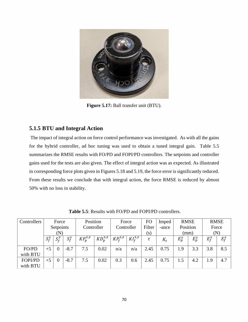
70

Figure 5.17: Ball transfer unit (BTU).

5.1.5 BTU and Integral Action

The impact of integral action on force control performance was investigated. As with all the gains

for the hybrid controller, ad hoc tuning was used to obtain a tuned integral gain. Table 5.5

summarizes the RMSE results with FO/PD and FOPI/PD controllers. The setpoints and controller

gains used for the tests are also given. The effect of integral action was as expected. As illustrated

in corresponding force plots given in Figures 5.18 and 5.19, the force error is significantly reduced.

From these results we conclude that with integral action, the force RMSE is reduced by almost

50% with no loss in stability.

Table 5.5: Results with FO/PD and FOPI/PD controllers.

Controllers Force

Setpoints

(N)

Position

Controller

Force

Controller

FO

Filter

(s)

Imped

-ance

RMSE

Position

(mm)

RMSE

Force

(N)

𝑆𝑓𝑥 𝑆𝑓

𝑦 𝑆𝑓

𝑧 𝐾𝑃𝑝𝑥,𝑧

𝐾𝐷𝑝𝑥,𝑧

𝐾𝑃𝑓𝑥,𝑧

𝐾𝐼𝑓𝑥,𝑧

𝜏 𝐾𝑡 𝐸𝑝𝑥 𝐸𝑝

𝑧 𝐸𝑓𝑥 𝐸𝑓

𝑧

FO/PD

with BTU

+5 0 -8.7 7.5 0.02 n/a n/a 2.45 0.75 1.9 3.3 3.8 8.5

FOPI/PD

with BTU

+5 0 -8.7 7.5 0.02 0.3 0.6 2.45 0.75 1.5 4.2 1.9 4.7

71

Figure 5.18: Force error with FO/PD hybrid controller and BTU.

Figure 5.19: Force error with FOPI/PD hybrid controller and BTU.

72

5.1.6 Tuned FO/PD Control

Table 5.6 summarizes the RMSE result with FO/PD control with tuned time constant and

impedance. The setpoints and other controller gains used for this test are also given. This result

gives the lowest RMSE by tuning time constant to 2.45 and impedance to 0.25. The corresponding

plots of position error and force are given in Figure 5.20 and 5.21. The tuning tests that were

conducted to obtain this result are given in Appendix D specifically Figures D.1 to D.4

Table 5.6: Best result with hybrid FO/PD controller

Force Setpoints

(N)

Position

Controller

FO

Filter

(s)

Imped

-ance

RMSE

Position

(mm)

RMSE

Force

(N)

𝑆𝑓𝑥 𝑆𝑓

𝑦 𝑆𝑓

𝑧 𝐾𝑃𝑝𝑥,𝑧

𝐾𝐷𝑝𝑥,𝑧

𝜏 𝐾𝑡 𝐸𝑝𝑥 𝐸𝑝

𝑧 𝐸𝑓𝑥 𝐸𝑓

𝑧

+5 0 -8.7 7.5 0.02 2.45 0.25 1.7 2.4 5.7 3.9

73

Figure 5.20: Position error for X and Z axis with tuned FO/PD control.

Figure 5.21: Force result for X and Z axis with tuned FO/PD control.

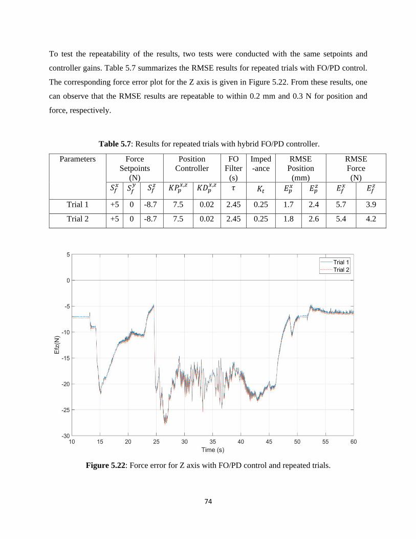
74

To test the repeatability of the results, two tests were conducted with the same setpoints and

controller gains. Table 5.7 summarizes the RMSE results for repeated trials with FO/PD control.

The corresponding force error plot for the Z axis is given in Figure 5.22. From these results, one

can observe that the RMSE results are repeatable to within 0.2 mm and 0.3 N for position and

force, respectively.

Table 5.7: Results for repeated trials with hybrid FO/PD controller.

Figure 5.22: Force error for Z axis with FO/PD control and repeated trials.

Parameters Force

Setpoints

(N)

Position

Controller

FO

Filter

(s)

Imped

-ance

RMSE

Position

(mm)

RMSE

Force

(N)

𝑆𝑓𝑥 𝑆𝑓

𝑦 𝑆𝑓

𝑧 𝐾𝑃𝑝𝑥,𝑧

𝐾𝐷𝑝𝑥,𝑧

𝜏 𝐾𝑡 𝐸𝑝𝑥 𝐸𝑝

𝑧 𝐸𝑓𝑥 𝐸𝑓

𝑧

Trial 1 +5 0 -8.7 7.5 0.02 2.45 0.25 1.7 2.4 5.7 3.9

Trial 2 +5 0 -8.7 7.5 0.02 2.45 0.25 1.8 2.6 5.4 4.2

75

5.2 BW/PD Control Results

The effect of replacing the FO filter with a second order Butterworth (BW) filter was examined.

Table 5.8 summarizes the RMSE results with BW/PD control with three different passband edge

frequencies. The setpoints and controller gains used for the tests are also given. The corresponding

plots for force and position for all the three tests are given in Appendix D (refer to Figures D.5 to

D.9). From the results we conclude that Test 1 with fp set to 6.3 gives the lowest position error and

Test 2 with fp set to 12.6 gives the lowest force error. Higher impedance of 3.33 gives better results

but then it becomes more of a position control than force control which reduces the effect of the

filter on force regulation. The best performance with the BW filter was obtained when the cutoff

frequency was set to 15 Hz which gave a passband edge frequency of 12.6 Hz and a time constant

of 0.06 sec. The force error increases significantly when there is high increase in passband edge

frequency as shown in Test 3 and which causes higher degree of oscillation. Recall that the time

constant for the FO filter was 2.45 sec. Tests with the BW filter demonstrated no significant

improvement in performance relative to the FO filter.

Table 5.8: Control parameters for hybrid BW/PD controller.

Parameters Force Setpoints

(N)

Position

Controller

Passband

Edge

Frequency

(Hz)

Imped

-ance

RMSE

Position

(mm)

RMSE

Force

(N)

𝑆𝑓𝑥 𝑆𝑓

𝑦 𝑆𝑓

𝑧 𝐾𝑃𝑝𝑥,𝑧

𝐾𝐷𝑝𝑥,𝑧

fp 𝐾𝑡 𝐸𝑝𝑥 𝐸𝑝

𝑧 𝐸𝑓𝑥 𝐸𝑓

𝑧

Test 1 +5 0 -8.7 7.5 0.02 6.3 3.33 2.4 8.3 8.3 17

Test 2 +5 0 -8.7 7.5 0.02 12.6 3.33 2.5 8.6 7.3 10.1

Test 3 +5 0 -8.7 7.5 0.02 63 3.33 2.8 8.7 8.9 19.7

76

5.3 PI/PD Control Results

The effect of replacing the FO filter with a PI controller was examined. Recall that the original

recommendation of Zeng and Hemani [15] was to use a hybrid controller that employed PI for

force control and PD for position control. The PI controller was tuned for the lowest force error

with an already tuned PD position controller (given in Appendix D, refer to Figures D.9 to D.12).

Tables 5.9 and 5.10 summarizes the RMSE results with PI/PD control with three different

proportional and integral gains of PI controller. The setpoints and controller gains used for the

tests are also given. The corresponding plots for force error are given in the Figures 5.23, 5.24,

5.27 and 5.28. From the results we conclude that, Test 9 with proportional gain of 0.5 gives lowest

force error for X axis and Test 8 with proportional gain of 0.3 gives lowest force error for Z axis.

In the same way, Test 11 with integral gain of 0.6 gives lowest force error for both X and Z axis.

For better visual understanding, the force plots are filtered in Figures 5.25, 5.26, 5.29 and 5.30.

Table 5.9: Tuning results of KPf for hybrid PI/PD controller.

Table 5.10: Tuning results of KIf for hybrid PI/PD controller.

Parameters Force

Setpoints

(N)

Position

Controller

Force

Controller

Imped

-ance

RMSE

Position

(mm)

RMSE

Force

(N)

𝑆𝑓𝑥 𝑆𝑓

𝑦 𝑆𝑓

𝑧 𝐾𝑃𝑝𝑥,𝑧

𝐾𝐷𝑝𝑥,𝑧

𝐾𝑃𝑓𝑥,𝑧

𝐾𝐼𝑓𝑥,𝑧

𝐾𝑡 𝐸𝑝

𝑥 𝐸𝑝𝑧 𝐸𝑓

𝑥 𝐸𝑓𝑧

Test 7 +5 0 -8.7 7.5 0.02 0.1 0 2 2.3 8.3 12.8 21.3

Test 8 +5 0 -8.7 7.5 0.02 0.3 0 2 2.5 8.2 11 19

Test 9 +5 0 -8.7 7.5 0.02 0.5 0 2 2.7 8.2 9.3 22

Parameters Force

Setpoints

(N)

Position

Controller

Force Controller Imped

-ance

RMSE

Position

(mm)

RMSE

Force

(N)

𝑆𝑓𝑥 𝑆𝑓

𝑦 𝑆𝑓

𝑧 𝐾𝑃𝑝𝑥,𝑧

𝐾𝐷𝑝𝑥,𝑧

𝐾𝑃𝑓𝑥 𝐾𝑃𝑓

𝑧 𝐾𝐼𝑓𝑥,𝑧

𝐾𝑡 𝐸𝑝

𝑥 𝐸𝑝𝑧 𝐸𝑓

𝑥 𝐸𝑓𝑧

Test 10 +5 0 -8.7 7.5 0.02 0.5 0.3 0.2 2 2.2 8.3 12.6 19.8

Test 11 +5 0 -8.7 7.5 0.02 0.5 0.3 0.6 2 2.2 8.3 7 16.2

Test 12 +5 0 -8.7 7.5 0.02 0.5 0.3 1 2 2.3 8.3 7.8 16.4

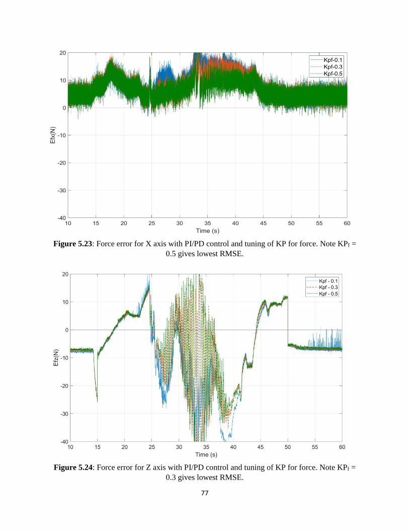
77

Figure 5.23: Force error for X axis with PI/PD control and tuning of KP for force. Note KPf =

0.5 gives lowest RMSE.

Figure 5.24: Force error for Z axis with PI/PD control and tuning of KP for force. Note KPf =

0.3 gives lowest RMSE.

78

Figure 5.25: Force error for X axis with PI/PD control and tuning of KP for force. Note KPf =

0.5 gives lowest RMSE. (filtered data)

Figure 5.26: Force error for Z axis with PI/PD control and tuning of KP for force. Note KPf =

0.3 gives lowest RMSE.

79

Figure 5.27: Force error for X axis with PI/PD control and tuning of KI for force. Note KIf = 0.6

gives lowest RMSE.

Figure 5.28: Force error for Z axis with PI/PD control and tuning of KI for force. Note KIf = 0.6

gives lowest RMSE.

80

Figure 5.29: Force error for X axis with PI/PD control and tuning of KI for force. Note KIf = 0.6

gives lowest RMSE. (filtered data)

Figure 5.30: Force error for Z axis with PI/PD control and tuning of KI for force. Note KIf = 0.6

gives lowest RMSE. (filtered data)

81

5.4 FOPI/PD Control Results

Tests were conducted in which the FO filter was added to the PI force controller to see if

performance could be improved. Table 5.11 summarizes the RMSE results with PI/PD and

FOPI/PD controllers. The setpoints and controller gains used for the tests are also given. The

corresponding plots of position and force error are given in Figures 5.31 to 5.34. From these results

we conclude that adding FO filter to PI control improves the force and position RMSE for X and

Z axis by a significant amount.

Table 5.11: Comparison of FO/PD and FOPI/PD controllers.

Hybrid

Controller

Force

Setpoints

(N)

Position

Controller

Force

Controller

FO

Filter

(s)

Imped

-ance

RMSE

Position

(mm)

RMSE

Force

(N)

𝑆𝑓𝑥 𝑆𝑓

𝑦 𝑆𝑓

𝑧 𝐾𝑃𝑝𝑥,𝑧

𝐾𝐷𝑝𝑥,𝑧

𝐾𝑃𝑓𝑥,𝑧

𝐾𝐼𝑓𝑥,𝑧

𝜏 𝐾𝑡 𝐸𝑝𝑥 𝐸𝑝

𝑧 𝐸𝑓𝑥 𝐸𝑓

𝑧

PI/PD +5 0 -8.7 7.5 0.02 0.3 0.6 2.45 0.25 6.1 8.4 12.1 10.5

FOPI/PD +5 0 -8.7 7.5 0.02 0.3 0.6 2.45 0.25 5.9 7.2 8.7 9.3

82

Figure 5.31: Position error for X axis with different force controllers. FOPI controller gives the

lowest RMSE.

Figure 5.32: Position error for Z axis with different force controllers. FOPI controller gives the

lowest RMSE.

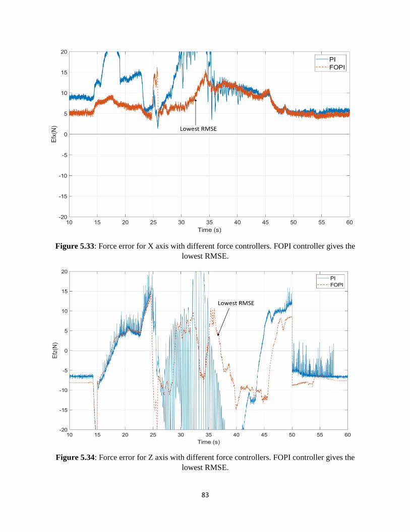
83

Figure 5.33: Force error for X axis with different force controllers. FOPI controller gives the

lowest RMSE.

Figure 5.34: Force error for Z axis with different force controllers. FOPI controller gives the

lowest RMSE.

84

5.5 Comparison of Tuned Results

The performance results for the four tuned hybrid controllers are tabulated in Table 5.12 and given

graphically in Figure 5.35. The individual test plots are given as Figures 5.36 to 5.39. The FO/PD

hybrid controller gave the best force regulation results, with the lowest RMSEs for the force in

both axes (6 and 3.6, respectively). The PI/PD hybrid controller gave the best position regulation

results, with the lowest RMSEs for the position in both axes (2.5 and 8.2, respectively).

Table 5.12: Tuned set of control parameters for different controllers.

Figure 5.35: Comparison of position and force error (X and Z axes) of the tuned results.

Hybrid

Controller

Force

Setpoints

(N)

Position

Controller

Force

Controller Filter

(s)

Imped

-ance

RMSE

Position

(mm)

RMSE

Force

(N)

𝑆𝑓𝑥 𝑆𝑓

𝑦 𝑆𝑓

𝑧 𝐾𝑃𝑝𝑥,𝑧

𝐾𝐷𝑝𝑥,𝑧

𝐾𝑃𝑓𝑥,𝑧

𝐾𝐼𝑓𝑥,𝑧

𝜏 𝐾𝑡 𝐸𝑝𝑥 𝐸𝑝

𝑧 𝐸𝑓𝑥 𝐸𝑓

𝑧

FO/PD +5 0 -8.7 7.5 0.02 - - 2.45 0.25 1.7 2.4 5.7 3.9

BW/PD +5 0 -8.7 7.5 0.02 - - 0.06 3.33 2.5 8.6 7.3 10.1

PI/PD +5 0 -8.7 7.5 0.02 0.3 0.6 - 0.5 1.6 2.2 9.7 17.2

FOPI/PD +5 0 -8.7 7.5 0.02 0.3 0.8 2.45 0.25 6.3 6.7 7.4 8.1

85

Figure 5.36: Position error for X axis comparing tuned result of controllers. PI controller gives

the lowest RMSE.

Figure 5.37: Position error for Z axis comparing tuned result of controllers. PI controller gives

the lowest RMSE.

86

Figure 5.38: Force error for X axis comparing tuned result of controllers. FO filter gives the

lowest RMSE. (filtered data)

Figure 5.39: Force error for Z axis comparing tuned result of controllers. FO filter gives the

lowest RMSE. (filtered data)

87

By comparing these four controllers, we can conclude that PI/PD controller has better position

control and FO/PD controller has better force control.

5.6 Summary

The performance of a hybrid controller with PD for position control and four different force

controllers was studied. The output of the force controller was input to the position controller by

way of an impedance factor. Each controller was tuned in the same ad hoc fashion in order to

provide a fair comparison of performance. The four force controllers were FO filter, BW filter, PI

and FOPI. The effect of different trajectories and different contact angles was examined.

From Section 5.1, the effect of impedance on position and force was observed. As the impedance

is increased, the hybrid controller gives better position control and as it is decreased, it gives better

force control. Also, results with sander at 30 deg to the bowl is better than at 45 and maintains

better surface contact. In the tests using ball transfer unit, the position error was decreased to less

than half of that when using the sander. Adding integral action to the force control reduced the

error by almost 50%.

From Section 5.2, it is evident that Butterworth filter results were not better compared to FO filter

results. The motion gets unstable with a small change in passband frequency. From Section 5.3

and 5.4, it was concluded that PI controller with tuned proportional and integral gains delivered

better results and adding first order filter improves performance still further.

As shown in Figure 5.35, the lowest position RMSE for both the x-axis and the z-axis was obtained

with PI action as the force controller (not the FO filter). But the quality of the sanding process is

determined by the force regulation and less so by the position regulation. Thus, the conclusion is

still that a FO filter for the force controller and PD action for the position controller gives the best

performance. It should be noted that this performance was obtained with only a rough trajectory

estimation of the bowl geometry as based on the bowl’s diameter and depth

88

CHAPTER 6

CONCLUSIONS AND RECOMMENDATIONS

This thesis set out to determine whether a serial robot could be used to sand a wooden bowl, in

order to free a human operator from what is considered a hazardous task. The hypothesis was that

a hybrid force/position impedance controller could sand the inside of a bowl, mimic the motions

and technique of the human operator, and be able to deal with conditions of unknown geometry.

There have been a number of previous studies on the sanding of wood, and even more studies on

the polishing of metal, but in the main they all relied on accurate dimensional data as obtained and

implemented through sophisticated CAD/CAM systems. The approach taken in this thesis

assumed that specific geometric information on the bowl was unavailable, aside from nominal

diameter and depth dimensions. This approach was consistent with the need for the system to

demonstrate an ability to deal with conditions of unknown geometry. It also was in-line with the

desire to keep the system as low cost as possible and avoid the need to laser or range scan every

bowl.

To test the hypothesis, an apparatus was assembled consisting of four main hardware components:

an articulated robot arm to mimic the motion of an operator (CRS A465 with six degrees of

freedom), a 3 axis force sensor to measure the contact forces (JR3), a lightweight compact sander

for the sanding action (3M pneumatic orbital) and a vacuum chuck to hold the wooden bowl in

place. The interface between the dedicated controller for the robot (C500C) and a desktop

computer (PC) had to be commissioned and debugged. The control program on the PC was written

in MATLAB/Simulink. An accurate kinematic model of a robotic arm was developed and

validated in order to generate the individual motor motions required for the end effector to follow

the desired point by point trajectory, while maintaining the orientation of the sander at a constant

angle of relative to the surface of the bowl.

89

The arm was programmed to follow a radial line from the rim of the bowl to its center and then

back to the rim. A hybrid force/position impedance controller was implemented. Proportional

Derivative (PD) action was adopted for the position controller. Four different force controllers

were tested: First Order (FO) filter, Butterworth filter, Proportional Integral (PI) control and

combined FO/PI control. Tuning tests were conducted to obtain the best values for the controller

gains. Root Mean Squared Error (RMSE) was used as a quantitative performance measure. The

effect of sander angle and the nature of the trajectory was tested.

6.1 Conclusions

It was concluded that the sander should be held at an angle of 30 deg relative to the surface of the

bowl, with an applied normal force of 10 N. The robot should be programmed to follow a trajectory

that starts at the bowl’s rim and traces the interior surface of the bowl along radial lines towards

the centre of the bowl. These conditions produced the best performance and came closest to

mimicking the technique of a human operator.

The experimental results indicated that the FO filter as the force controller gave the best result,

with the lowest force RMSE for both the x-axis and the z-axis. The lowest position RMSE for both

the x-axis and the z-axis was obtained with PI action as the force controller (not the FO filter). But

the quality of the sanding process is determined by the force regulation and less so by the position

regulation. Thus, the conclusion is still that a FO filter for the force controller and PD action for

the position controller gives the best performance. It should be reemphasized that this performance

was obtained with only a rough trajectory estimation of the bowl’s geometry. A precise CAD/CAM

model of the bowl was not employed.

6.2 Contributions

The contributions of the thesis can be summarized as follows:

• A test apparatus has been assembled and commissioned that enables future work on the

subject of robot-based sanding of wooden products

90

• An updated kinematics and dynamics model of a CRS A465 robot has been developed

and validated and is available for other researchers

• The ability of a hybrid force/position impedance controller, with a FO-based force

controller and a PD-based position controller, to sand a wooden bowl with only nominal

dimensional data has been demonstrated

6.3 Recommendations

It remains to be seen as to whether performance could be improved still further with a more

advanced hybrid impedance controller. For example, one that uses fuzzy logic, to account for the

variable nature of the friction forces [17]. Future work could include the introduction of a friction

model to enable a more sophisticated setpoint for the force. Operationally, a rotating vacuum chuck

could be added to incrementally rotate the bowl as the sander travels along radial lines. This would

be the mechanism for sanding the entire inside surface of the bowl. Another recommendation

would be to mount the arm in inverted position. This would open up the available workspace,

eliminate possible singularities and enable alternate trajectories, such as a spiral.

It would also be helpful if there was an objective measure of sanding quality. At the moment,

sanding quality is measured subjectively by visual and tactile inspection with a human operator.

Finally, additional experiments should be conducted with additional wooden bowls of different

sizes with different geometries in order to evaluate the robustness of the controller.

91

REFERENCES

1. Healthwise Staff. (2018, September 20). Wrist Care: Preventing Carpal Tunnel Syndrome.

Retrieved from https://www.healthlinkbc.ca/health-topics/tn9041

2. Bend Plating. (2018, February 5). What Is Robotic Polishing and Why Is It Important?

Retrieved from https://www.bendplating.com/robotic-polishing-important/

3. Takeuchi, Y., Asakawa, N. and GE, D. (1993). Automation of Polishing Work by an

Industrial Robot. In JSME Int. Journal, Series C, 36(40): 556-561.

4. Nagata, F., Hase, T., Haga, Z., Watanabe, K. and Omoto, M. (2007). CAD/CAM – based

Position/Force Controller for a Mold Polishing Robot. Journal of Mechatronics, 17(4-5):

207-216.

5. Nagata, F., Kusumoto, Y., Fujimoto, Y. and Watanabe, K. (2007). Robotic Sanding System

for new Designed Furniture with Free-Formed Surface. Journal of Robotics and Computer

Integrated Manufacturing, 23(4): 371-379.

6. Takeuchi, Y., GE, D. and Asakawa, N. (1993). Automated Polishing Process with a

Human-like Dexterous Robot. Proceedings of the IEEE conference on Robotics and

Automation, 3: 950-956.

7. Mohsin, I., He, K., Li. Z. and Du, R. (2019). Path Planning under Force Control in Robotic

Polishing of the Complex Curved Surfaces. Applied Sciences, 9(24), 5489.

8. Lee, M.C., Go, S.J., Jung, J.Y. and Lee, M.H. (1999). Development of a User-friendly

Polishing Robot System. Proceedings of the IEEE International conference on Intelligent

Robots and Systems, 3: 1914-1919.

9. Tian, F., Lv, C., Li, Z. and Liu, G. (2016). Modeling and Control of Robotic Automatic

Polishing for Curved Surfaces. CIRP Journal of Manufacturing Science and Technology,

14: 55-64.

10. Tian, F., Lv, C., Li, Z. and Liu, G. (2016). Polishing Pressure Investigations of Robot

Automatic Polishing on Curved Surfaces. International Journal of Advanced

Manufacturing Technology, 87 (1-4): 639-646.

92

11. Huang, T., Li, C., Wang, Z., Liu, Y. and Chen, G. (2016). A Flexible System of Complex

Surface Polishing based on the Analysis of the Contact Force and Path Research. IEEE

Workshop on Advanced Robotics and its Social Impacts (ARSO). 289-293

12. Tsai, L.-W. (2005). Robot analysis: the mechanics of serial and parallel manipulators.

New York: John Wiley & Sons, 60-91.

13. Kinsheel, A., Taha, Z., Deboucha, A. and Tuan Mohd Yusoff, T.Y. (2012). Robust least

square estimation of the CRS A465 robot arm’s dynamic model parameters. Journal of

Mechanical Engineering Research, 4(3): 89–99.

14. Radkhah, K., Kulic, D. and Croft, E. (2007). Dynamic Parameter Identification for the CRS

A460 Robot. Proceedings of the IEEE/RSJ International Conference on Intelligent Robots

and Systems San Diego, 3842-3847.

15. Zeng, G. and Hemami, A. (1997). An Overview of Robot Force Control. Journal of

Robotica, New York, 15(5): 473-482.

16. Mohan, C., Surgenor, B.W., Monteiro, L. and Nazari, V. (2017). Tracking with a Fuzzy

Logic Controller as Applied to a Pneumatic Robot for Polishing. Proceedings of the 30th

IEEE Cdn. Conf. Electrical and Computer Engineering (CCECE), 1-6

17. Raibert, M. H. and Craig, J., J. (1981). Hybrid Position/Force Control of Manipulators.

Journal of Dynamic Systems, Measurements and Control (ASME), 102: 126-133.

18. De Gea, J. and Kirchner, F. (2008). Modelling and Simulation of Robot Arm Interaction

Forces using Impedance Control. Proceedings of the 17th World Congress, 08: 15589-

15594.

19. Komati, B., Pac, M.R., Clévy, C., Popa, D.O., & Lutz, P. (2013). Explicit force control

V.S. impedance control for micromanipulation. ASME-IDETC International Design

Engineering Technical Conferences & Computers and Information in Engineering

Conference, 1: 1-8.

20. Heinrichs, B., Sepheri, N. and Thorton-Trump, A. B. (1997). Position-Based Impedance

Control of an Industrial Hydraulic Manipulator. Proceedings of the IEEE International

Conference on Robotics and Automation, 97: 46-52.

21. Eppinger, S. D. and Seering, W.P. (1987). Understanding Bandwidth Limitations in Robot

Force Control. Proceedings of the IEEE International Conference on Robotics and

Automation, 4: 904-909.

93

22. Application Environment, 1st ed., CRS Robotics CO., Burlington, ON, CA, 1999, 25-32.

23. CRS A465 Robot Arm User Guide, 2nd ed., CRS Robotics CO., Burlington, ON, CA, 1999.

6-74.

24. C500 Controller User Guide, 2nd ed., CRS Robotics CO., Burlington, ON, CA, 2000. 4-

36.

25. Teach Pendant, 1st ed., CRS Robotics CO., Burlington, ON, CA, 1999. 11-21.

26. Quanser /CRS Model A465 Open Architecture Robot, 2nd ed., Quanser Consulting Inc.,

Markham, ON, CA, 2001, 12-25

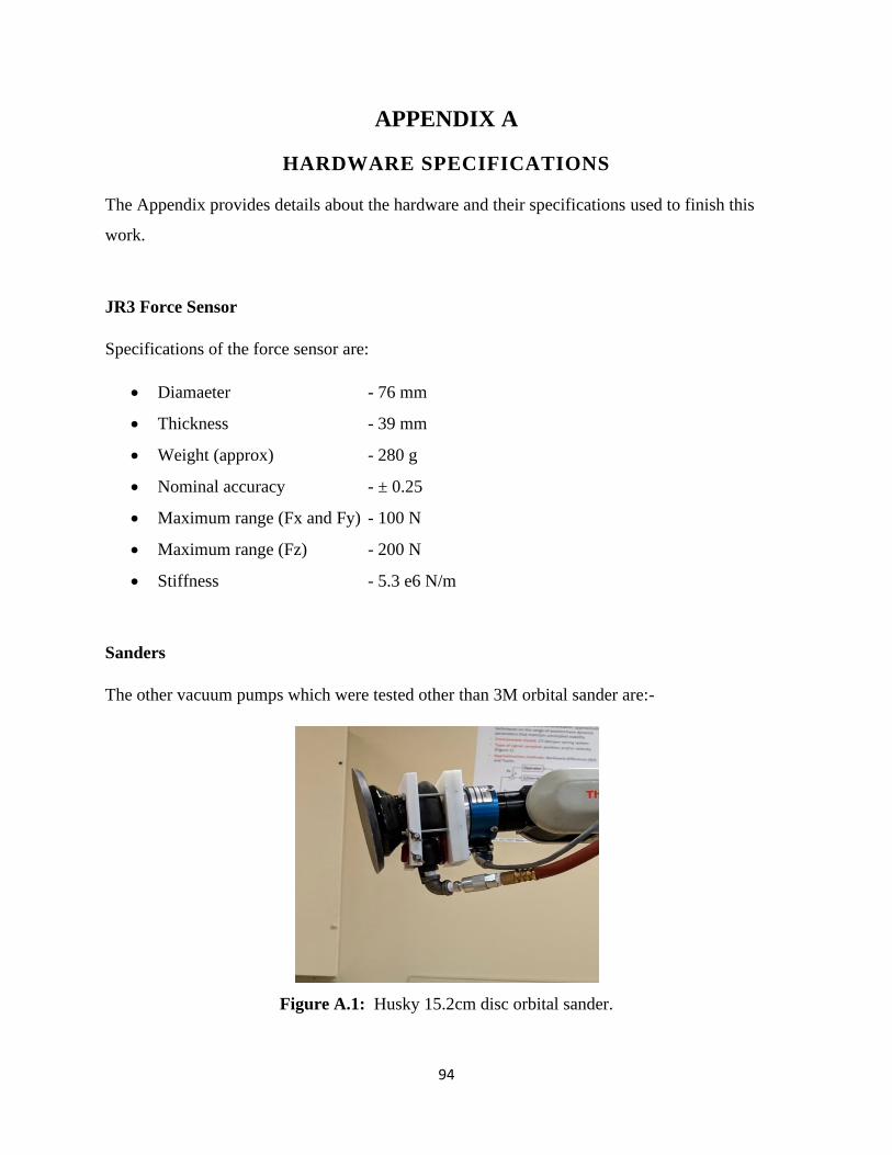
94

APPENDIX A

HARDWARE SPECIFICATIONS

The Appendix provides details about the hardware and their specifications used to finish this

work.

JR3 Force Sensor

Specifications of the force sensor are:

• Diamaeter - 76 mm

• Thickness - 39 mm

• Weight (approx) - 280 g

• Nominal accuracy - ± 0.25

• Maximum range (Fx and Fy) - 100 N

• Maximum range (Fz) - 200 N

• Stiffness - 5.3 e6 N/m

Sanders

The other vacuum pumps which were tested other than 3M orbital sander are:-

Figure A.1: Husky 15.2cm disc orbital sander.

95

Figure A.2: Bosch orbital sander.

Vacuum Pump

Specifications of the vacuum pump (GAST) are:

• Power - 1/4 hp (0.19 kW)

• Max Pressure (50 Hz) - 10 psi (0.7 bar)

• Max Pressure (60 Hz) - 10 psi (0.7 bar)

• Max Vacuum (60 Hz) - 26.5 in-Hg (116.0 mbar abs)

• Weight - 32 lbs (15 kg)

• Min Temperature - 33.8 °F (1 °C)

• Max Temperature - 104 °F (40 °C)

JUN-AIR Compressor

It is a highly efficient and quiet compressor used to power the pnematic sander in this application.

It is normally used in dental offices since it is very quiet. The air pressure of the compressor is

maintained at 80 psi during sanding with the help of the regulator and yellow handle (shown in

Figure A.3) is used to release the air to the sander.

96

Figure A.3: JUN-AIR compressor.

Specifications:

• Motor: - 0.68 kW / 0.92 HP

• Displacement (theoretical values): -100 l/min / 3.53 cu.ft/min

• Power consumption @ 8 bar: -5.8 Amps

• Max. Pressure: -8 bar / 120 psi

• Tank Size: -20 L / 5.3 US Gal

• Weight: -50 kg / 112 lbs

• Noise Level, Only: -48 dBA at 1m

97

Fig

ure

A.4

: S

hop d

raw

ing f

or

adap

ter

pla

te.

98

APPENDIX B

DYNAMICS EQUATIONS

The mass and inertia terms in the matrix D(q) (Section 4.5 - Robot Dynamics) are:

𝑑11 = 𝐼1𝑦𝑦 + 𝑚2𝑙𝑐22 + 𝐼2𝑦𝑦 + 𝑚3𝑎2

2 cos(𝑞2)2 + 𝐼2𝑥𝑥 sin(𝑞2)

2 + 𝑚3𝑙𝑐32 + 𝐼3𝑥𝑥 sin(𝑞2 + 𝑞3)

2

+ 𝑚3𝑎2𝑙𝑐3 sin(2𝑞2 + 𝑞3) + 𝐼3𝑧𝑧 cos(𝑞2 + 𝑞3)2

+ 𝑚4𝑙𝑐42 + 𝐼4𝑦𝑦 cos(𝑞4)

2 + 𝑚5𝑙𝑐52 + 𝐼5𝑦𝑦 sin(𝑞5)

2 + 𝐼5𝑥𝑥 sin(𝑞5)2 + 𝑚6𝑙𝑐6

2

+ 𝐼6𝑥𝑥 cos(𝑞4 + 𝑞6)2 + 𝐼6𝑦𝑦 cos(𝑞4 + 𝑞6)

2 + 𝑚5𝑑42 sin(𝑞4)

2

+ 2𝑚6𝑑4𝑙𝑐6 cos(𝑞4 + 𝑞6)

𝑑22 = 𝑚2𝑙𝑐22 + 𝐼2𝑧𝑧 + 𝑚3𝑎2

2 + 𝑚3𝑙𝑐32 + 𝐼3𝑦𝑦 + 2𝑚3𝑎2𝑙𝑐3 sin(𝑞3)

+ 𝑚4𝑙𝑐42 + 𝐼4𝑦𝑦 cos(𝑞4)

2 + 𝑚5𝑙𝑐52 + 𝐼5𝑦𝑦 sin(𝑞5)

2 + 𝐼5𝑥𝑥 sin(𝑞5)2 + 𝑚6𝑙𝑐6

2

+ 𝐼6𝑥𝑥 cos(𝑞4 + 𝑞6)2 + 𝐼6𝑦𝑦 cos(𝑞4 + 𝑞6)

2 + 𝑚5𝑑42 sin(𝑞4)

2

+ 2𝑚6𝑑4𝑙𝑐6 cos(𝑞4 + 𝑞6)

𝑑23 = 𝑑32 = 𝑚3𝑙𝑐32 + 𝐼3𝑦𝑦 + 𝑚3𝑎2𝑙𝑐3 sin(𝑞3) + 𝑚4𝑙𝑐4

2 + 𝑚5𝑑42 + 𝑚6𝑑4𝑙𝑐6 cos(𝑞4 + 𝑞6)

𝑑33 = 𝑚3𝑙𝑐32 + 𝐼3𝑦𝑦 + 𝑚4𝑙𝑐4

2 + 𝐼4𝑦𝑦 + 𝐼4𝑥𝑥 cos(𝑞4)2 + 𝑚5𝑙𝑐5

2 + 𝐼5𝑦𝑦 sin(𝑞5)2 + 𝐼5𝑥𝑥 sin(𝑞5)

2

+ 𝑚6𝑙𝑐62 + 𝐼6𝑥𝑥 cos(𝑞4 + 𝑞6)

2 + 𝐼6𝑦𝑦 cos(𝑞4 + 𝑞6)2 + 𝑚5𝑑4

2 sin(𝑞4)2

+ 2𝑚6𝑑4𝑙𝑐6 cos(𝑞4 + 𝑞6)

𝑑34 = 𝑑43 = 𝑚4𝑙𝑐42 + 𝐼4𝑦𝑦 + 𝑚3𝑑4

2 sin(𝑞3)2 + 𝐼4𝑥𝑥 cos(𝑞4)

2 + 𝑚6𝑑4𝑙𝑐6 cos(𝑞4 + 𝑞6)

𝑑35 = 𝑑53 = 𝑚5𝑙𝑐52 + 𝐼5𝑦𝑦 + 𝑚5𝑑4

2 sin(𝑞4)2 + 𝑚5𝑑4

2 + 𝐼5𝑥𝑥 sin(𝑞5)2

𝑑36 = 𝑑63 = 𝑚6𝑙𝑐62 + 𝐼6𝑧𝑧 + 𝑚6𝑑4𝑙𝑐6 cos(𝑞4 + 𝑞6) + 𝐼6𝑥𝑥 cos(𝑞4 + 𝑞6)

2

𝑑24 = 𝑑42 = 𝑚4𝑙𝑐42 + 𝐼4𝑥𝑥 cos(𝑞4)

2 + 𝑚2𝑑42 sin(𝑞2)

2 + 𝑚5𝑑4𝑙𝑐5 sin(𝑞5) + 𝐼6𝑥𝑥 cos(𝑞4 + 𝑞6)2

𝑑44 = 𝑚4𝑙𝑐42 + 𝐼4𝑦𝑦 + 𝑚5𝑙𝑐5

2 + 𝐼5𝑦𝑦 sin(𝑞5)2 + 𝐼5𝑥𝑥 sin(𝑞5)

2 + 𝑚6𝑙𝑐62 + 𝐼6𝑥𝑥 cos(𝑞4 + 𝑞6)

2

+ 𝐼6𝑦𝑦 cos(𝑞4 + 𝑞6)2 + 𝑚5𝑑4

2 sin(𝑞4)2 + 2𝑚6𝑑4𝑙𝑐6 cos(𝑞4 + 𝑞6)

𝑑45 = 𝑑54 = 𝑚5𝑙𝑐52 + 𝐼5𝑦𝑦 + 𝑚5𝑑4

2 sin(𝑞4)2

𝑑46 = 𝑑64 = 𝑚6𝑙𝑐62 + 𝐼6𝑧𝑧 + 𝑚6𝑑4

2 cos(𝑞4)2

99

𝑑25 = 𝑑52 = 𝐼5𝑦𝑦 + 𝑚5𝑙𝑐52 + 𝑚5𝑑4𝑙𝑐5 sin(𝑞5) + 𝐼4𝑥𝑥 cos(𝑞4)

2 + 𝐼6𝑥𝑥 cos(𝑞4 + 𝑞6)2

𝑑26 = 𝑑62 = 𝐼6𝑦𝑦 + 𝑚6𝑙𝑐62 + 𝐼6𝑥𝑥 cos(𝑞4 + 𝑞6)

2

𝑑55 = 𝑚5𝑙𝑐52 + 𝑚5𝑑4

2 + 𝐼5𝑦𝑦 + 𝑚6𝑙𝑐62 + 𝐼6𝑧𝑧 + 𝑚5𝑑4𝑙𝑐5 sin(𝑞5)

𝑑56 = 𝑑65 = 𝑚6𝑙𝑐62 + 𝐼6𝑧𝑧 + 𝐼6𝑥𝑥 cos(𝑞6)

2

𝑑66 = 𝑚6𝑙𝑐62 + 𝐼6𝑧𝑧

The Coriolis and Centrifugal terms in the matrix C(𝑞, �̇�) (Section 4.5 - Robot Dynamics) are:

(where 𝑠𝑖𝑐𝑖 = sin(𝑞𝑖) cos(𝑞𝑖); 𝑠𝑖𝑗𝑐𝑖𝑗 = sin(𝑞𝑖 + 𝑞𝑗) cos(𝑞𝑖 + 𝑞𝑗))

𝑐11 = (−𝑚3𝑎22𝑠2𝑐2 + 𝐼2𝑥𝑥𝑠2𝑐2 + 𝐼3𝑥𝑥𝑠23𝑐23 − 𝐼3𝑧𝑧𝑠23𝑐23 + 𝑚3𝑎2𝑙𝑐3 cos(2𝑞2 + 𝑞3))�̇�2

+ (𝐼3𝑥𝑥𝑠23𝑐23 +1

2𝑚3𝑎2𝑙𝑐3 cos(2𝑞2 + 𝑞3) − 𝐼3𝑧𝑧𝑠23𝑐23)�̇�3 + (−𝐼4𝑦𝑦𝑠4𝑐4

− 𝐼6𝑥𝑥𝑠46𝑐46 − 𝐼6𝑦𝑦𝑠46𝑐46 + 𝑚5𝑑42𝑠4𝑐4 − 𝑚6𝑑4𝑙𝑐6𝑠46𝑐46)�̇�4 + (𝐼5𝑦𝑦𝑠5𝑐5

+ 𝐼5𝑥𝑥𝑠5𝑐5)�̇�5 − (𝐼6𝑥𝑥𝑠46𝑐46 + 𝐼6𝑦𝑦𝑠46𝑐46 + 𝑚6𝑑4𝑙𝑐6𝑠46𝑐46)�̇�6

𝑐12 = −𝑐21 = (−𝑚3𝑎22𝑠2𝑐2 + 𝐼2𝑥𝑥𝑠2𝑐2 + 𝐼3𝑥𝑥𝑠23𝑐23 + 𝑚3𝑎2𝑙𝑐3 cos(2𝑞2 + 𝑞3) − 𝐼3𝑧𝑧𝑠23𝑐23)�̇�2

𝑐13 = −𝑐31 = (𝐼3𝑥𝑥𝑠23𝑐23 +1

2𝑚3𝑎2𝑙𝑐3 cos(2𝑞2 + 𝑞3) − 𝐼3𝑧𝑧𝑠23𝑐23)�̇�3

𝑐14 = −𝑐41 = (−𝐼4𝑦𝑦𝑠4𝑐4 − 𝐼6𝑥𝑥𝑠46𝑐46 − 𝐼6𝑦𝑦𝑠46𝑐46 + 𝑚5𝑑42𝑠4𝑐4 − 𝑚6𝑑4𝑙𝑐6𝑠46𝑐46)�̇�4

𝑐15 = −𝑐51 = (𝐼5𝑦𝑦𝑠5𝑐5 + 𝐼5𝑥𝑥𝑠5𝑐5)�̇�5

𝑐16 = −𝑐61 = (−𝐼6𝑥𝑥𝑠46𝑐46 − 𝐼6𝑦𝑦𝑠46𝑐46 − 𝑚6𝑑4𝑙𝑐6𝑠46𝑐46)�̇�6

𝑐22 = 2𝑚3𝑎2𝑙𝑐3𝑠3𝑐3�̇�3+ (𝐼4𝑦𝑦𝑠4𝑐4 − 𝐼6𝑥𝑥𝑠46𝑐46 − 𝐼6𝑦𝑦𝑠46𝑐46 + 𝑚5𝑑42𝑠4𝑐4 − 𝑚6𝑑4𝑙𝑐6𝑠46𝑐46)�̇�4

+ (𝐼5𝑦𝑦𝑠5𝑐5 + 𝐼5𝑥𝑥𝑠5𝑐5)�̇�5 + (−𝐼6𝑥𝑥𝑠46𝑐46 − 𝐼6𝑦𝑦𝑠46𝑐46 − 𝑚6𝑑4𝑙𝑐6𝑠46𝑐46)�̇�6

𝑐23 = −𝑐32 = (−𝑚6𝑑4𝑙𝑐6𝑠46) �̇�4

𝑐24 = (2𝑚2𝑑42𝑠2𝑐2 + 𝐼4𝑦𝑦𝑠4𝑐4 + 𝐼6𝑥𝑥𝑠46𝑐46) �̇�2 + 𝑚3𝑎2𝑙𝑐3𝑐3�̇�3 + (𝑚5𝑑4𝑙𝑐5𝑐5 + 𝐼4𝑦𝑦𝑠4𝑐4

+ 𝐼6𝑥𝑥𝑠46𝑐46)�̇�5

100

𝑐25 = −𝑐52 = (𝐼5𝑦𝑦𝑠5𝑐5 + 𝐼5𝑥𝑥𝑠5𝑐5) �̇�2 − (𝐼4𝑦𝑦𝑠4𝑐4 + 𝐼6𝑥𝑥𝑠46𝑐46 + 𝑚5𝑑4𝑙𝑐5𝑐5)�̇�4 +

(𝑚5𝑑4𝑙𝑐5𝑐5 + 𝐼4𝑦𝑦𝑠4𝑐4 + 𝐼6𝑥𝑥𝑠46𝑐46)�̇�5 − 𝐼6𝑥𝑥𝑠46𝑐46�̇�6

𝑐26 = −𝑐62 = (−𝐼6𝑥𝑥𝑠46𝑐46 − 𝐼6𝑦𝑦𝑠46𝑐46 − 𝑚6𝑑4𝑙𝑐6𝑠46𝑐46)�̇�2− 𝑚6𝑑4𝑙𝑐6𝑠46 �̇�3 +

−2𝐼6𝑥𝑥𝑠46𝑐46�̇�4 + 𝐼6𝑥𝑥𝑠46𝑐46�̇�5

𝑐33 = (−𝐼4𝑥𝑥𝑠4𝑐4 + 𝑚5𝑑42𝑠4𝑐4 − 𝐼6𝑥𝑥𝑠46𝑐46 − 𝐼6𝑦𝑦𝑠46𝑐46 − 𝑚6𝑑4𝑙𝑐6𝑠46𝑐46)�̇�4 + (𝐼5𝑦𝑦𝑠5𝑐5

+ 𝐼5𝑥𝑥𝑠5𝑐5)�̇�5 + (−𝐼6𝑥𝑥𝑠46𝑐46 − 𝐼6𝑦𝑦𝑠46𝑐46 − 𝑚6𝑑4𝑙𝑐6𝑠46𝑐46)�̇�6

𝑐34 = −𝑐43 = (−𝑚6𝑑4𝑙𝑐6𝑠46) �̇�2 + (2𝑚3𝑑42𝑠3𝑐3 − 𝐼4𝑦𝑦𝑠4𝑐4 − 𝐼6𝑥𝑥𝑠46𝑐46 − 𝐼6𝑦𝑦𝑠46𝑐46 +

𝑚5𝑑42𝑠4𝑐4 − 𝑚6𝑑4𝑙𝑐6𝑠46𝑐46)�̇�3 + 𝑚5𝑑4

2𝑠4𝑐4�̇�5 − 𝐼6𝑥𝑥𝑠46𝑐46�̇�6

𝑐35 = −𝑐53 = (−𝐼5𝑦𝑦𝑠5𝑐5 + 𝐼5𝑥𝑥𝑠5𝑐5)�̇�3 + 𝑚5𝑑42𝑠4𝑐4�̇�4

𝑐36 = −𝑐63 = (−𝑚6𝑑4𝑙𝑐6𝑠46𝑐46)�̇�2 + (𝐼6𝑥𝑥𝑠46𝑐46 + 𝐼6𝑦𝑦𝑠46𝑐46 + 𝑚6𝑑4𝑙𝑐6𝑠46𝑐46)�̇�3

+ 𝐼6𝑥𝑥𝑠46𝑐46�̇�5

𝑐44 = (𝐼6𝑥𝑥𝑠46𝑐46 + 𝐼6𝑦𝑦𝑠46𝑐46 + 𝑚6𝑑4𝑙𝑐6𝑠46𝑐46 − 𝑚5𝑑42𝑠4𝑐4)�̇�4 + (𝐼5𝑦𝑦𝑠5𝑐5 + 𝐼5𝑥𝑥𝑠5𝑐5)�̇�5

− (𝐼6𝑥𝑥𝑠46𝑐46 + 𝐼6𝑦𝑦𝑠46𝑐46 + 𝑚6𝑑4𝑙𝑐6𝑠46𝑐46)�̇�6

𝑐42 = (𝐼4𝑦𝑦𝑠4𝑐4 − 𝐼6𝑥𝑥𝑠46𝑐46 − 𝐼6𝑦𝑦𝑠46𝑐46 + 𝑚5𝑑42𝑠4𝑐4 − 𝑚6𝑑4𝑙𝑐6𝑠46𝑐46)�̇�2 − 𝑚6𝑑4𝑙𝑐6𝑠46�̇�3

+ 2(−𝐼4𝑦𝑦𝑠4𝑐4 − 𝐼6𝑥𝑥𝑠46𝑐46)�̇�4 + (𝑚5𝑑4𝑙𝑐5𝑐5 + 𝐼4𝑦𝑦𝑠4𝑐4 + 𝐼6𝑥𝑥𝑠46𝑐46)�̇�5

− 2𝐼6𝑥𝑥𝑠46𝑐46�̇�6

𝑐45 = −𝑐54 = −(𝑚5𝑑4𝑙𝑐5𝑐5 + 𝐼4𝑦𝑦𝑠4𝑐4 + 𝐼6𝑥𝑥𝑠46𝑐46)�̇�2 + 𝑚5𝑑42𝑠4𝑐4�̇�3 + (𝐼5𝑦𝑦𝑠5𝑐5

+ 𝐼5𝑥𝑥𝑠5𝑐5)�̇�4

𝑐46 = −𝑐64 = −𝐼6𝑥𝑥𝑠46𝑐46�̇�3 − (𝑚6𝑑42𝑠4𝑐4 + 𝐼6𝑥𝑥𝑠46𝑐46 + 𝐼6𝑦𝑦𝑠46𝑐46 + 𝑚6𝑑4𝑙𝑐6𝑠46𝑐46)�̇�4

+ (𝐼6𝑥𝑥𝑠46𝑐46 + 𝐼6𝑦𝑦𝑠46𝑐46 + 𝑚6𝑑4𝑙𝑐6𝑠46𝑐46)�̇�6

𝑐55 = 𝑚5𝑑4𝑙𝑐5𝑠5�̇�5

𝑐56 = −𝑐65 = −𝐼6𝑥𝑥𝑠46𝑐46�̇�2

𝑐66 = 0

101

APPENDIX C

SIMULINK BLOCKS

The Simulink blocks used to program the robot are shown in the Figures A.4 to A.19.

102

Fig

ure

C.1

: S

imuli

nk m

odel

use

d t

o p

rogra

m t

he

A465 a

rm.

103

Figure C.2: Blocks used to send the trajectory in world coordinates. (Desired position block)

Figure C.3: Sub-blocks inside the inverse kinematics block.

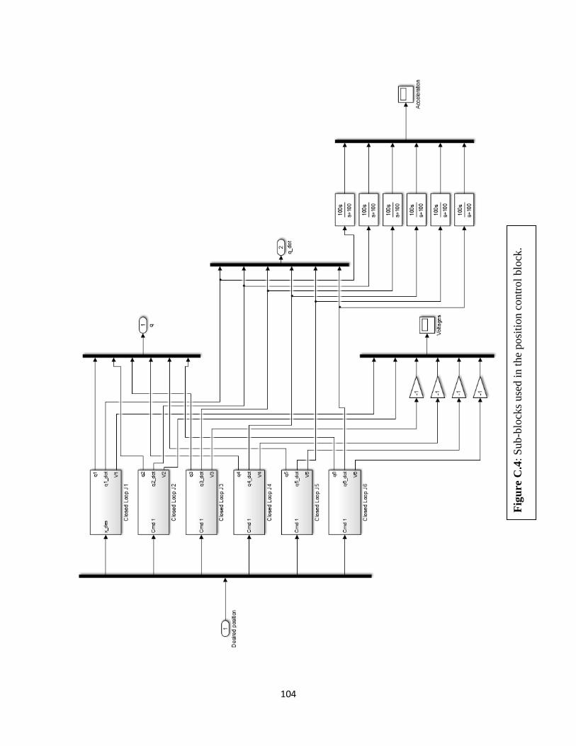
104

Fig

ure

C.4

: S

ub

-blo

cks

use

d i

n t

he

posi

tion c

ontr

ol

blo

ck.

105

Figure C.5: Sub-blocks inside the closed loop block of joint 1.

Figure C.6: Sub-blocks inside the joint 1 block.

106

Figure C.7: Sub-blocks inside the PD controller1 block.

Figure C.8: Sub-blocks inside the force control block in main Simulink model.

107

Figure C.9: Sub-blocks inside the FO filter block.

Figure C.10: Sub-blocks inside the PI controller block.

Figure C.11: Sub-blocks inside the Butterworth filter block

108

Figure C.12: Blocks present in CRS_takeover block which is used to switch between OA and

CRS mode of the arm.

Figure C.13: Sub-blocks inside the angle to coordinates block.

109

Fig

ure

C.1

4:

Sub

-blo

cks

in e

nco

der

rea

din

gs

blo

ck use

d t

o c

om

par

e th

e ac

tual

and d

esir

ed t

raje

ctory

.

110

Figure C.15: Sub-blocks in home block

Figure C.16: The sub-blocks included in the forward kinematics block.

111

APPENDIX D

TUNING PLOTS

The tuning plots of first order filter and Butterworth filter (which are not shown in the results

chapter) are given below:

Table D.1 summarizes the RMSE results with FO/PD control with three different time constants.

The setpoints and controller gains used for the tests are also given. The corresponding plots for

force and position errors are given in Figures D.1 to D.4. From these results we conclude that Test

2 (𝜏 = 2.45) gives the lowest RMSE for position and force compared to other two tests.

Table D.1: Tuning time constant (𝜏) for hybrid FO/PD controller.

The Butterworth filter results are given in Table 5.8 and the corresponding plots are given in

Figures D.5 to D.8. Test 2 is the best result with lowest force error.

Parameters Force Setpoints

(N)

Position

Controller

FO

Filter

(s)

Imped

-ance

RMSE

Position

(mm)

RMSE

Force

(N)

𝑆𝑓𝑥 𝑆𝑓

𝑦 𝑆𝑓

𝑧 𝐾𝑃𝑝𝑥,𝑧

𝐾𝐷𝑝𝑥,𝑧

𝜏 𝐾𝑡 𝐸𝑝𝑥 𝐸𝑝

𝑧 𝐸𝑓𝑥 𝐸𝑓

𝑧

Test 1 +5 0 -8.7 7.5 0.02 1.5 0.25 3.6 4.7 14.7 14.2

Test 2 +5 0 -8.7 7.5 0.02 2.45 0.25 1.7 2.4 5.7 3.9

Test 3 +5 0 -8.7 7.5 0.02 3.5 0.25 12 9.6 11.1 10.3

112

Figure D.1: Position error for X axis with FO/PD control and tuning of time constant. Note

𝜏 = 2.45 gives lowest RMSE.

Figure D.2: Position error for Z axis with FO/PD control and tuning of time constant. Note 𝜏 =

2.45 gives lowest RMSE.

113

Figure D.3: Force error for X axis with FO/PD control and tuning of time constant. Note 𝜏 =

2.45 gives lowest RMSE.

Figure D.4: Force error for Z axis with FO/PD control and tuning of time constant. Note 𝜏 =

2.45 gives lowest RMSE.

114

Figure D.5: Position error for X axis with BW/PD control and tuning of fp. Note fp = 6.3 gives

lowest RMSE.

Figure D.6: Position error for Z axis with BW/PD control and tuning of fp. Note fp = 6.3 gives

lowest RMSE.

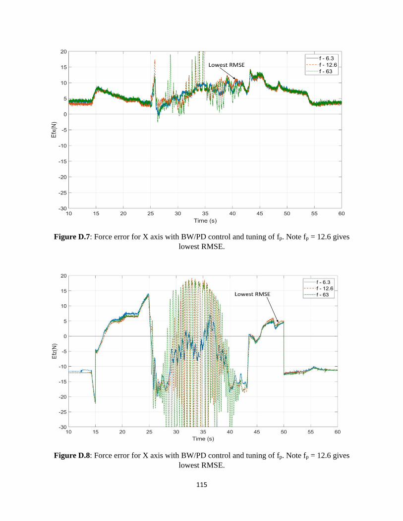
115

Figure D.7: Force error for X axis with BW/PD control and tuning of fp. Note fp = 12.6 gives

lowest RMSE.

Figure D.8: Force error for X axis with BW/PD control and tuning of fp. Note fp = 12.6 gives

lowest RMSE.

116

Tables D.2 and D.3 summarizes the RMSE results with PI/PD control with three different

proportional and derivative gains of PD controller. The setpoints and controller gains used for the

tests are also given. The corresponding plots for position error are given in in Figures D.9 to D.12.

From the results we conclude that, Test 2 with proportional gain of 7.5 gives lowest position error

for both X and Z axis. In the same way, Test 5 with derivative gain of 0.02 gives lowest position

error for X axis and Test 6 with derivative gain of 0.1 gives lowest position error for Z axis.

Table D.2: Tuning results of KPp for PD controller.

Table D.3: Tuning results of KDp for PD controller.

Parameters Force

Setpoints

(N)

Position

Controller

Force

Controller

Imped

-ance

RMSE

Position

(mm)

RMSE

Force

(N)

𝑆𝑓𝑥 𝑆𝑓

𝑦 𝑆𝑓

𝑧 𝐾𝑃𝑝𝑥,𝑧

𝐾𝐷𝑝𝑥,𝑧

𝐾𝑃𝑓𝑥,𝑧

𝐾𝐼𝑓𝑥,𝑧

𝐾𝑡 𝐸𝑝𝑥 𝐸𝑝

𝑧 𝐸𝑓𝑥 𝐸𝑓

𝑧

Test 1 +5 0 -8.7 2.5 0 0.3 0.8 2 3.3 4.7 12.9 16.5

Test 2 +5 0 -8.7 7.5 0 0.3 0.8 2 1.9 1.4 12.1 14.1

Test 3 +5 0 -8.7 12.5 0 0.3 0.8 2 16.8 9.4 19.8 19.1

Parameters Force

Setpoints

(N)

Position

Controller

Force

Controller

Imped

-ance

RMSE

Position

(mm)

RMSE

Force

(N)

𝑆𝑓𝑥 𝑆𝑓

𝑦 𝑆𝑓

𝑧 𝐾𝑃𝑝𝑥,𝑧

𝐾𝐷𝑝𝑥,𝑧

𝐾𝑃𝑓𝑥,𝑧

𝐾𝐼𝑓𝑥,𝑧

𝐾𝑡 𝐸𝑝𝑥 𝐸𝑝

𝑧 𝐸𝑓𝑥 𝐸𝑓

𝑧

Test 4 +5 0 -8.7 7.5 0.001 0.3 0.8 2 5.3 2.9 15.5 17.4

Test 5 +5 0 -8.7 7.5 0.02 0.3 0.8 2 2.8 1.4 8.2 11.8

Test 6 +5 0 -8.7 7.5 0.1 0.3 0.8 2 8.3 1.2 8.3 10.6

117

Figure D.9: Position error for X axis with PI/PD control and tuning of KP for position. Note KPP

= 7.5 gives lowest RMSE.

Figure D.10: Position error for Z axis with PI/PD control and tuning of KP for position. Note

KPP = 7.5 gives lowest RMSE.

118

Figure D.11: Position error for X axis with PI/PD control and tuning of KD for position. Note

KD = 0.02 gives lowest RMSE.

Figure D.12: Position error for Z axis with PI/PD control and tuning of KD for position. Note

KD = 0.02 gives lowest RMS

119

APPENDIX E

MATLAB CODE

Initially there was a Simulink model bug “U1077” for the inverse kinematics block which

prevented compilation and gave an error of “illegal transform” for certain angle inputs as given

below:

NMAKE: fatal error U1077: '"c:\Program Files (x86)\Microsoft Visual Studio10.0\VC\bin\amd64\

cl.exe"' : return code '0x2' Stop.

This issue was related to “Joint Angles to World Coordinates” block C code which terminates the

simulation within few seconds. To correct this bug, “Joint Angles to World coordinates” block

was rewritten from scratch as shown below. Fixing this bug took considerable time.

#ifndef __kin465_h__

#define __kin465_h__

#include <math.h>

/**************/

/* Constants */

/**************/

#define PI (3.141592653589793) /* = pi */

#define PID2 (1.570796326794896) /* = pi/2 */

#define PIX2 (6.283185307179586) /* = pi*2 */

#define SQRT2 (1.41421356237) /* = sqrt(2) */

#define EPSILON (0.001)

#define DEGtoRAD (0.01745329252) /* = pi/180.0 */

#define RADtoDEG (57.2957795131) /* = 180.0/pi */

#define NUM_AXES 6 /* can change if extra axes are desired */

#define XFORM_SIZE 12

#define NUM_SOLN 8 /* number of possible kinematics configurations */

#define POSITIVE (1)

#define NEGATIVE (-1)

#define NO_SOLUTION (-1)

/* Robot Parameters */

#define A2 (304.8) /* 12.0 in -- length of link 2 */

120

#define D4 (330.2) /* 13.0 in -- length of link 3 */

/* pose-related symbols */

#define REACH_BACK(x) (!(x & REACH_BIT))

#define ELBOW_UP(x) (x & ELBOW_BIT )

#define WRIST_FLIP(x) (!(x & WRIST_BIT))

#define REACH_BIT 0x01

#define ELBOW_BIT 0x02

#define WRIST_BIT 0x08

#define FREE_REACH_BIT 0x10

#define FREE_ELBOW_BIT 0x20

#define FREE_WRIST_BIT 0x40

#define WRIST_FREE(x) (x & FREE_WRIST_BIT)

#define ELBOW_FREE(x) (x & FREE_ELBOW_BIT)

#define REACH_FREE(x) (x & FREE_REACH_BIT)

/* indicies into homogeneous transform matrix*/

#define r11 0 /* was Nx */

#define r21 4 /* was Ny */

#define r31 8 /* was Nz */

#define r12 1 /* was Bx */

#define r22 5 /* was By */

#define r32 9 /* was Bz */

#define r13 2 /* was Ax */

#define r23 6 /* was Ay */

#define r33 10 /* was Az */

#define Px 3

#define Py 7

#define Pz 11

/* indicies into cartesian location array*/

#define XDIM 0

#define YDIM 1

#define ZDIM 2

#define YAW 3 /* Oc */

#define PITCH 4 /* Ac */

#define ROLL 5 /* Tc */

/* indicies into joint array */

#define J1 0

#define J2 1

#define J3 2

#define J4 3

#define J5 4

#define J6 5

121

/* indicies into joint solution matrix */

#define FUN 0

#define FUF 1

#define FDN 2

#define FDF 3

#define BUN 4

#define BUF 5

#define BDN 6

#define BDF 7

/* note that the last 4 elements of all transform matricies are implied */

#define IDENTITY_MATRIX {1,0,0,0,0,1,0,0,0,0,1,0}

#define SHOULDER_MATRIX {1,0,0,0,0,1,0,0,0,0,1,330.2}

#define INV_SHOULDER_MATRIX {1,0,0,0,0,1,0,0,0,0,1,-330.2}

#define FLANGE_MATRIX {0,0,-1,0,0,1,0,0,1,0,0,76.2}

#define INV_FLANGE_MATRIX {0,0,1,-76.2,0,1,0,0,-1,0,0,0}

/* return code definitions */

#define OK 0x00

#define JOINT_OUT_OF_RANGE 0x01

#define ILLEGAL_TRANSFORM 0x02

#define INVKIN_OUTOFREACH 0x03

#define CASE_ERROR 0x04

/*********************/

/* Type Declarations */

/*********************/

typedef double Float; /* can be changed to double precision if desired */

typedef unsigned int word;

typedef struct

{

Float joint[NUM_AXES];

}

Joint_Solution ;

/*************************/

/* Function declarations */

/*************************/

/* in kin465.c */

void A465_joint_to_world(Float* joint_angles, Float* world_coords);

int A465_world_to_joint(word stance, Float* old_joint_angles, Float* world_coords, Float*

joint_angles);

void A465_joint_to_motor(Float *joint_angles, int *motor_pulses);

void A465_motor_to_joint(int *motor_pulses, Float *joint_angles);

int A465_user_joint_check(Float *user_joints);

122

int A465_stance( Float *joint_angle, word oldstance, word *newstance );

/* in crsutils.c */

void matrix_mult(Float *_A, Float *_B, Float *_C);

void convert_worldcoords_to_homotransform(Float *worldcoords, Float *homotransform);

void convert_homotransform_to_worldcoords(Float *homotransform, Float *worldcoords);

Float map_to_PI( Float in_angle );

/* in A465params.c */

void A465_get_joint_limits(Float **poslim, Float **neglim);

void A465_get_transmission_factor(Float **transfactor);

void A465_get_inv_transmission_factor(Float **invtransfactor);

void A465_get_trans_ratio(Float **transratio);

void get_base_offset(Float **base_offset);

void get_inv_base_offset(Float **inv_base_offset);

void get_tool_offset(Float **tool_offset);

void get_inv_tool_offset(Float **inv_tool_offset);

#endif

#include "kin465.h"

static Float A465_posjointlim[NUM_AXES] = { 3.0000, 1.571, 2.007, 3.1416, 1.8325,

3.1416};

static Float A465_negjointlim[NUM_AXES] = {-3.0000,-1.571, -2.007, -3.1416,-1.8325, -

3.1416};

static Float A465_trans_ratio[NUM_AXES] = {100, 100, -100, -101,-100, -101}; /* Harmonic

drive gear ratios*/

static Float A465_trans_factor[NUM_AXES] = {6.2831853e-5, 6.2831853e-5, -6.2831853e-5, -

1.2441951e-4, -1.2566371e-4, -1.2441951e-4};

static Float A465_inv_trans_factor[NUM_AXES]= {15915.494, 15915.494, -15915.494, -

8037.3246, -7957.7471, -8037.3246};

/*static int A465_enc_resolution[NUM_AXES]= {1000, 1000, 1000, 500, 500, 500}; */

/* the following can be changed to include a base or tool offset */

static Float A465_basematrix[XFORM_SIZE] = IDENTITY_MATRIX;

static Float A465_inv_basematrix[XFORM_SIZE] = IDENTITY_MATRIX;

static Float A465_toolmatrix[XFORM_SIZE] = IDENTITY_MATRIX;

static Float A465_inv_toolmatrix[XFORM_SIZE] = IDENTITY_MATRIX;

/* A465_get_joint_limits() returns a pointer to the array of positive

* and negative joint limits of the A465 robot */

void A465_get_joint_limits(Float **poslim, Float **neglim)

{

*poslim = A465_posjointlim;

*neglim = A465_negjointlim;

return;

}

123

/* A465_get_transmission_factor() returns a pointer to the array of transmission factors.

* These factors are used to convert from motor coordinates to joint angles

* and are calculated as follows:

* trans = 1/[(Encoder pulses per motor turn) * (motor turns per radian of joint motion)]

*/

void A465_get_transmission_factor(Float **transfactor)

{

*transfactor = A465_trans_factor;

return;

}

/* A465_get_inv_transmission_factor() returns a pointer to the array of inverse

* transmission factors. These factors are used to convert from joint angles to

* motor coordinates and are calculated as follows:

* invtrans = (Encoder pulses per motor turn) * (motor turns per radian of joint motion)

*/

void A465_get_inv_transmission_factor(Float **invtransfactor)

{

*invtransfactor = A465_inv_trans_factor;

return;

}

/* A465_get_trans_ratio() a pointer to the array of transmission ratios.

* The transmission ratio is the ratio used to convert from

* motor revolutions to joint angles (in radians)

*/

void A465_get_trans_ratio(Float **transratio)

{

*transratio = A465_trans_ratio;

return;

}

/* Each of the following 4 routines are stubs to eventually allow

* for base and tool transforms. Each currently return a pointer

* to the identity transform.

*/

void get_base_offset(Float **base_offset)

{

*base_offset = A465_basematrix;

}

void get_inv_base_offset(Float **inv_base_offset)

{

*inv_base_offset = A465_inv_basematrix;

}

void get_tool_offset(Float **tool_offset)

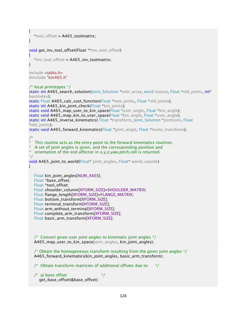
124

{

*tool_offset = A465_toolmatrix;

}

void get_inv_tool_offset(Float **inv_tool_offset)

{

*inv_tool_offset = A465_inv_toolmatrix;

}

include <stdio.h>

#include "kin465.h"

/* local prototypes */

static int A465_search_solution(Joint_Solution *soln_array, word stance, Float *old_joints, int*

bestindex);

static Float A465_calc_cost_function(Float *new_joints, Float *old_joints);

static int A465_kin_joint_check(Float *kin_joints);

static void A465_map_user_to_kin_space(Float *user_angle, Float *kin_angle);

static void A465_map_kin_to_user_space(Float *kin_angle, Float *user_angle);

static int A465_inverse_kinematics( Float *transform, Joint_Solution *jointsoln, Float

*old_joints);

static void A465_forward_kinematics(Float *joint_angle, Float *homo_transform);

/*

* This routine acts as the entry point to the forward kinematics routines.

* A set of joint angles is given, and the corresponding position and

* orientation of the end affector in x,y,z,yaw,pitch,roll is returned.

*/

void A465_joint_to_world(Float* joint_angles, Float* world_coords)

{

Float kin_joint_angles[NUM_AXES];

Float *base_offset;

Float *tool_offset;

Float shoulder_column[XFORM_SIZE]=SHOULDER_MATRIX;

Float flange_length[XFORM_SIZE]=FLANGE_MATRIX;

Float bottom_transform[XFORM_SIZE];

Float terminal_transform[XFORM_SIZE];

Float arm_without_terminal[XFORM_SIZE];

Float complete_arm_transform[XFORM_SIZE];

Float basic_arm_transform[XFORM_SIZE];

/* Convert given user joint angles to kinematic joint angles */

A465_map_user_to_kin_space(joint_angles, kin_joint_angles);

/* Obtain the homogeneous transform resulting from the given joint angles */

A465_forward_kinematics(kin_joint_angles, basic_arm_transform);

/* Obtain transform matricies of additional offsets due to: */

/* a) base offset */

get_base_offset(&base_offset);

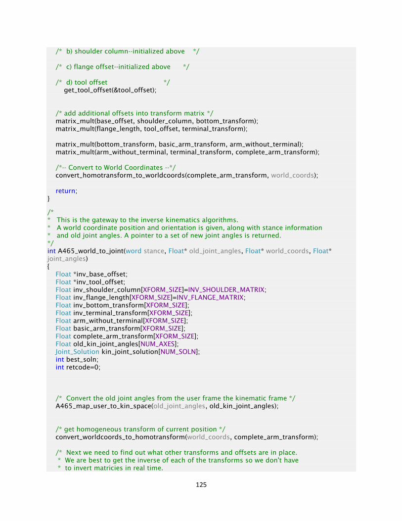
125

/* b) shoulder column--initialized above */

/* c) flange offset--initialized above */

/* d) tool offset */

get_tool_offset(&tool_offset);

/* add additional offsets into transform matrix */

matrix_mult(base_offset, shoulder_column, bottom_transform);

matrix_mult(flange_length, tool_offset, terminal_transform);

matrix_mult(bottom_transform, basic_arm_transform, arm_without_terminal);

matrix_mult(arm_without_terminal, terminal_transform, complete_arm_transform);

/*-- Convert to World Coordinates --*/

convert_homotransform_to_worldcoords(complete_arm_transform, world_coords);

return;

}

/*

* This is the gateway to the inverse kinematics algorithms.

* A world coordinate position and orientation is given, along with stance information

* and old joint angles. A pointer to a set of new joint angles is returned.

*/

int A465_world_to_joint(word stance, Float* old_joint_angles, Float* world_coords, Float*

joint_angles)

{

Float *inv_base_offset;

Float *inv_tool_offset;

Float inv_shoulder_column[XFORM_SIZE]=INV_SHOULDER_MATRIX;

Float inv_flange_length[XFORM_SIZE]=INV_FLANGE_MATRIX;

Float inv_bottom_transform[XFORM_SIZE];

Float inv_terminal_transform[XFORM_SIZE];

Float arm_without_terminal[XFORM_SIZE];

Float basic_arm_transform[XFORM_SIZE];

Float complete_arm_transform[XFORM_SIZE];

Float old_kin_joint_angles[NUM_AXES];

Joint_Solution kin_joint_solution[NUM_SOLN];

int best_soln;

int retcode=0;

/* Convert the old joint angles from the user frame the kinematic frame */

A465_map_user_to_kin_space(old_joint_angles, old_kin_joint_angles);

/* get homogeneous transform of current position */

convert_worldcoords_to_homotransform(world_coords, complete_arm_transform);

/* Next we need to find out what other transforms and offsets are in place.

* We are best to get the inverse of each of the transforms so we don't have

* to invert matricies in real time.

126

* */

/* a) inverse base offset */

get_inv_base_offset(&inv_base_offset);

/* b) inverse shoulder column--initialized above */

/* c) inverse flange offset--initialized above */

/* d) inverse tool offset */

get_inv_tool_offset(&inv_tool_offset);

/* Now strip off the extra transforms to leave only the transform between the

* intersection of joints 1&2 and joints 5&6. Result is the basic arm transform.

*/

matrix_mult(inv_shoulder_column, inv_base_offset, inv_bottom_transform);

matrix_mult(inv_tool_offset, inv_flange_length, inv_terminal_transform);

matrix_mult(complete_arm_transform, inv_terminal_transform, arm_without_terminal);

matrix_mult(inv_bottom_transform, arm_without_terminal, basic_arm_transform);

/* Call inverse kinematics to produce all possible joint solutions*/

retcode = A465_inverse_kinematics( basic_arm_transform, kin_joint_solution,

old_kin_joint_angles);

/* Bail out immediately if we have an invkin error */

if (retcode != OK)

return retcode;

/* Now, choose the appropriate solution according to given stance constraints*/

retcode = A465_search_solution( kin_joint_solution, stance, old_kin_joint_angles,

&best_soln);

if( retcode == OK)

{

/* We have a solution: convert joint angles to user frame */

A465_map_kin_to_user_space(&kin_joint_solution[best_soln].joint[J1], joint_angles);

}

else /* can not find a valid solution */

return(retcode);

return(OK );

}

/* Checks each joint to ensure that all are within joint limits.

* Returns OK if we're within the joint limits, or an error code

* indicating which joint is out of range.

* Note: based on user joint angles, NOT kinematic joint angles.

*/

127

int A465_user_joint_check(Float *user_joints)

{

Float *posjointlim;

Float *negjointlim;

int i;

A465_get_joint_limits(&posjointlim, &negjointlim);

for (i=0;i<NUM_AXES;i++)

{

/* check joint angle against limits */

if(( user_joints[i] > posjointlim[i]) || (negjointlim[i] > user_joints[i]))

{

/* joint out of range --send this back as an error */

return( -(JOINT_OUT_OF_RANGE | ((i + 1) << 4 ) ) );

}

}

return(OK);

}

/* A465_stance computes the robot configuration from the given joint angles.

* It takes the previous stance as an argument so that any free bits can be

* preserved in the result that is returned.

*/

int A465_stance( Float *joint_angle, word oldstance, word *newstance )

{

int singularity=0;

word tempstance;

Float kin_joint_angle[NUM_AXES];

Float s1,c1,s23,c2,px,py;

Float rtmp1, rtmp2, rtmp3;

Float etmp1;

Float wtmp1;

/*Init cfg to FUN (most common) stance --

* but preserve any free bits that are set

*/

tempstance = oldstance;

tempstance |= (REACH_BIT | ELBOW_BIT | WRIST_BIT);

/* convert from user to kin-space joint angles */

A465_map_user_to_kin_space(joint_angle, kin_joint_angle);

s1 = sin(kin_joint_angle[J1]);

c1 = cos(kin_joint_angle[J1]);

s23 = sin(kin_joint_angle[J2] + kin_joint_angle[J3] );

c2 = cos(kin_joint_angle[J2]);

/*-- Reach Forward/Back --*/

rtmp1 = -D4*s23 + A2*c2;

px = c1*rtmp1;

py = s1*rtmp1;

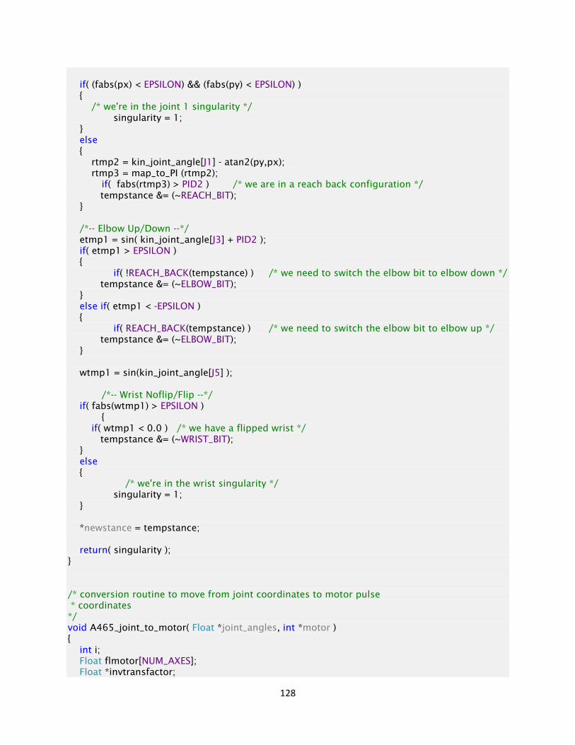
128

if( (fabs(px) < EPSILON) && (fabs(py) < EPSILON) )

{

/* we're in the joint 1 singularity */

singularity = 1;

}

else

{

rtmp2 = kin_joint_angle[J1] - atan2(py,px);

rtmp3 = map_to_PI (rtmp2);

if( fabs(rtmp3) > PID2 ) /* we are in a reach back configuration */

tempstance &= (~REACH_BIT);

}

/*-- Elbow Up/Down --*/

etmp1 = sin( kin_joint_angle[J3] + PID2 );

if( etmp1 > EPSILON )

{

if( !REACH_BACK(tempstance) ) /* we need to switch the elbow bit to elbow down */

tempstance &= (~ELBOW_BIT);

}

else if( etmp1 < -EPSILON )

{

if( REACH_BACK(tempstance) ) /* we need to switch the elbow bit to elbow up */

tempstance &= (~ELBOW_BIT);

}

wtmp1 = sin(kin_joint_angle[J5] );

/*-- Wrist Noflip/Flip --*/

if( fabs(wtmp1) > EPSILON )

{

if( wtmp1 < 0.0 ) /* we have a flipped wrist */

tempstance &= (~WRIST_BIT);

}

else

{

/* we're in the wrist singularity */

singularity = 1;

}

*newstance = tempstance;

return( singularity );

}

/* conversion routine to move from joint coordinates to motor pulse

* coordinates

*/

void A465_joint_to_motor( Float *joint_angles, int *motor )

{

int i;

Float flmotor[NUM_AXES];

Float *invtransfactor;

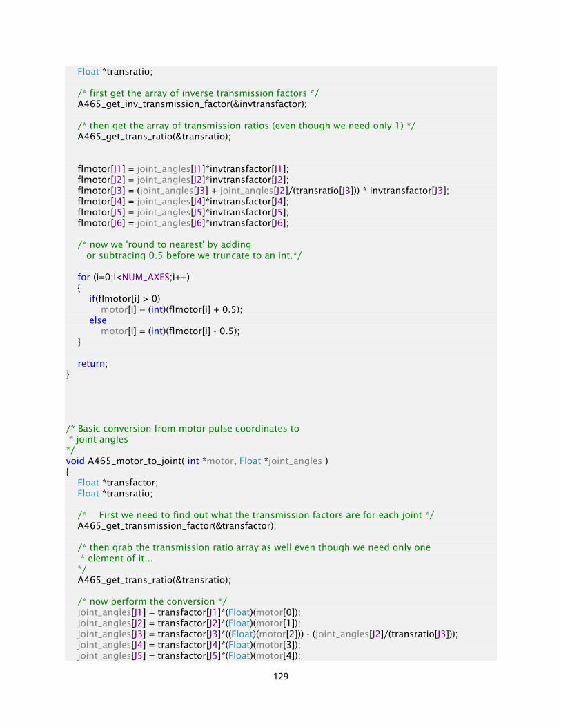
129

Float *transratio;

/* first get the array of inverse transmission factors */

A465_get_inv_transmission_factor(&invtransfactor);

/* then get the array of transmission ratios (even though we need only 1) */

A465_get_trans_ratio(&transratio);

flmotor[J1] = joint_angles[J1]*invtransfactor[J1];

flmotor[J2] = joint_angles[J2]*invtransfactor[J2];

flmotor[J3] = (joint_angles[J3] + joint_angles[J2]/(transratio[J3])) * invtransfactor[J3];

flmotor[J4] = joint_angles[J4]*invtransfactor[J4];

flmotor[J5] = joint_angles[J5]*invtransfactor[J5];

flmotor[J6] = joint_angles[J6]*invtransfactor[J6];

/* now we 'round to nearest' by adding

or subtracing 0.5 before we truncate to an int.*/

for (i=0;i<NUM_AXES;i++)

{

if(flmotor[i] > 0)

motor[i] = (int)(flmotor[i] + 0.5);

else

motor[i] = (int)(flmotor[i] - 0.5);

}

return;

}

/* Basic conversion from motor pulse coordinates to

* joint angles

*/

void A465_motor_to_joint( int *motor, Float *joint_angles )

{

Float *transfactor;

Float *transratio;

/* First we need to find out what the transmission factors are for each joint */

A465_get_transmission_factor(&transfactor);

/* then grab the transmission ratio array as well even though we need only one

* element of it...

*/

A465_get_trans_ratio(&transratio);

/* now perform the conversion */

joint_angles[J1] = transfactor[J1]*(Float)(motor[0]);

joint_angles[J2] = transfactor[J2]*(Float)(motor[1]);

joint_angles[J3] = transfactor[J3]*((Float)(motor[2])) - (joint_angles[J2]/(transratio[J3]));

joint_angles[J4] = transfactor[J4]*(Float)(motor[3]);

joint_angles[J5] = transfactor[J5]*(Float)(motor[4]);

130

joint_angles[J6] = transfactor[J6]*(Float)(motor[5]);

return;

}

/* ---------------------------------------local routines-----------------------------------------*/

/* A465_inverse_kinematics: Computes the kinematic joint angles 'jointsoln' from

* the basic arm transform 'transform'.

*

* Note: 'old_joints' is an array representing the robots current kinematic

* joint angles. It is used when a singularity is encountered in joint

* 1 (wrist directly above origin) or joint 5 (when J5 is exactly 0).

* In each case, we appeal to the previous joint angle for a reasonable

* approximation of where the next joint angle should be. Without an

* approach like this the arm may move erratically and dangerously.

*/

static int A465_inverse_kinematics( Float *transform, Joint_Solution *jointsoln, Float *old_joints)

{

Float linkvar1, linkvar2;

Float j1soln1, j1soln2;

Float s1, s1_F, s1_B, c1, c1_F, c1_B;

Float j3tmp1, j3tmp2, j3tmp3, j3tmp4;

Float j3soln1, j3soln2;

Float s3, c3_BUFD, c3_FUBD;

Float threespace_dist_sqr;

Float inv_3space_dist_sqr;

Float baseplane_dist;

Float j2tmp1_BUFD, j2tmp1_FUBD;

Float j2tmp1, j2tmp2;

Float s23, c23;

Float basedist_26;

Float j2soln;

Float j5_singularity;

Float s5, c5, s4, c4, s6, c6;

Float j4tmp1, j4tmp2, j4tmp3;

Float j4soln1, j4soln2;

Float j5soln1, j5soln2;

Float j6tmp1, j6tmp2;

Float j6soln1, j6soln2;

int index;

/* Joint 1 */

#ifndef TESTING

if( fabs(transform[Px]) < EPSILON && fabs(transform[Py]) < EPSILON )

{

/* we're in the joint 1 singularity directly above the origin */

j1soln1 = old_joints[J1];

j1soln2 = j1soln1 + PI;

}

else

#endif

{

j1soln1 = atan2(transform[Py],transform[Px]);

131

j1soln2 = j1soln1 + PI;

}

/* reach forward solutions */

jointsoln[FUN].joint[J1] = j1soln1;

jointsoln[FUF].joint[J1] = j1soln1;

jointsoln[FDN].joint[J1] = j1soln1;

jointsoln[FDF].joint[J1] = j1soln1;

/* reach backward solutions */

jointsoln[BUN].joint[J1] = j1soln2;

jointsoln[BUF].joint[J1] = j1soln2;

jointsoln[BDN].joint[J1] = j1soln2;

jointsoln[BDF].joint[J1] = j1soln2;

/* set up some variables for later */

s1_F=sin(j1soln1); /* forward */

c1_F=cos(j1soln1);

s1_B = -s1_F; /* backward */

c1_B = -c1_F;

/* Joint 3 */

linkvar1 = A2*A2+D4*D4;

linkvar2 = 4.0*A2*A2*D4*D4;

baseplane_dist = c1_F*transform[Px] + s1_F*transform[Py]; /* was f11p */

threespace_dist_sqr = baseplane_dist * baseplane_dist + transform[Pz] * transform[Pz];

j3tmp1 = linkvar1 - threespace_dist_sqr;

j3tmp2 = linkvar2 - j3tmp1*j3tmp1 ;

/* ensure we're within reach */

if( j3tmp2 < -linkvar2*EPSILON ) /* EPSILON defined in header file */

return( INVKIN_OUTOFREACH );

else if( j3tmp2 < 0.0 )

j3tmp2 = 0.0;

/* now determine the Joint 3 angle */

j3tmp3 = sqrt( j3tmp2 );

j3tmp4 = atan2( -j3tmp3,j3tmp1);

j3soln1 = PID2 + j3tmp4;

j3soln2 = PID2 - j3tmp4;

/* backward/up and forward/down solutions */

jointsoln[BUN].joint[J3] = j3soln1;

jointsoln[BUF].joint[J3] = j3soln1;

jointsoln[FDN].joint[J3] = j3soln1;

jointsoln[FDF].joint[J3] = j3soln1;

/* foward/up and backward/down solutions */

jointsoln[FUN].joint[J3] = j3soln2;

jointsoln[FUF].joint[J3] = j3soln2;

132

jointsoln[BDN].joint[J3] = j3soln2;

jointsoln[BDF].joint[J3] = j3soln2;

/* now prepare some variables for further stages. */

s3 =sin(j3soln1); /* was tmp2 */

c3_BUFD =cos(j3soln1); /* was tmp1 */

c3_FUBD = -c3_BUFD; /* same as cos(j3soln2) */

/* pre-calculating the inverse here saves cpu cycles later on */

inv_3space_dist_sqr = 1/threespace_dist_sqr;

/* Joint 2 --> Joint 6 */

/* set up joint 2 variables */

j2tmp1_BUFD = A2*c3_BUFD;

j2tmp1_FUBD = A2*c3_FUBD;

j2tmp2 = D4 - A2*s3;

/* We have two solutions for each of J1 and J3 (corresponding

* to reach forward/back and elbow up/down) so there are now a total of 4

* stance configurations that we can attain: FU, BU, FD, BD. We must find separate

* solutions for each configuration for all the remaining joints.

* To simplify this process we will loop through the following calculations

* 4 times, once for each of the configurations.

*/

/* Because of the way the solution array is organized, we must

* index through with a step size of two to hit each of the FU, BU

* FD, and BD solutions. See kin465.h for more info */

for (index=FUN;index<=6;index+=2)

{

switch(index)

{

case(FUN):

{

c1 = c1_F;

s1 = s1_F;

basedist_26 = baseplane_dist;

j2tmp1 = j2tmp1_FUBD;

break;

}

case(FDN):

{

c1 = c1_F;

s1 = s1_F;

basedist_26 = baseplane_dist;

j2tmp1 = j2tmp1_BUFD;

break;

}

case(BUN):

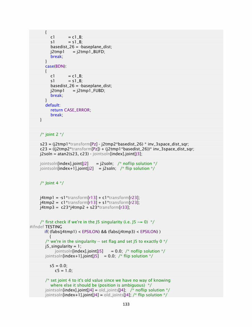
133

{

c1 = c1_B;

s1 = s1_B;

basedist_26 = -baseplane_dist;

j2tmp1 = j2tmp1_BUFD;

break;

}

case(BDN):

{

c1 = c1_B;

s1 = s1_B;

basedist_26 = -baseplane_dist;

j2tmp1 = j2tmp1_FUBD;

break;

}

default:

return CASE_ERROR;

break;

}

/* joint 2 */

s23 = (j2tmp1*transform[Pz] - j2tmp2*basedist_26) * inv_3space_dist_sqr;

c23 = ((j2tmp2*transform[Pz]) + (j2tmp1*basedist_26))* inv_3space_dist_sqr;

j2soln = atan2(s23, c23) - jointsoln[index].joint[J3];

jointsoln[index].joint[J2] = j2soln; /* noflip solution */

jointsoln[index+1].joint[J2] = j2soln; /* flip solution */

/* Joint 4 */

j4tmp1 = -s1*transform[r13] + c1*transform[r23];

j4tmp2 = c1*transform[r13] + s1*transform[r23];

j4tmp3 = c23*j4tmp2 + s23*transform[r33];

/* first check if we're in the J5 singularity (i.e. J5 ~= 0) */

#ifndef TESTING

if( (fabs(j4tmp1) < EPSILON) && (fabs(j4tmp3) < EPSILON) )

{

/* we're in the singularity -- set flag and set J5 to exactly 0 */

j5_singularity = 1;

jointsoln[index].joint[J5] = 0.0; /* noflip solution */

jointsoln[index+1].joint[J5] = 0.0; /* flip solution */

s5 = 0.0;

c5 = 1.0;

/* set joint 4 to it's old value since we have no way of knowing

where else it should be (position is ambiguous) */

jointsoln[index].joint[J4] = old_joints[J4]; /* noflip solution */

jointsoln[index+1].joint[J4] = old_joints[J4]; /* flip solution */

134

s4 = sin(old_joints[J4]);

c4 = cos(old_joints[J4]);

}

else

#endif

{

/* we're not singular in jt 5 */

j5_singularity = 0;

j4soln1 = atan2(j4tmp1,j4tmp3);

j4soln2 = j4soln1 + PI;

jointsoln[index+1].joint[J4] = j4soln1; /* wrist is flipped */

jointsoln[index].joint[J4] = j4soln2; /* wrist is not flipped */

s4 = sin(j4soln2);

c4 = cos(j4soln2);

}

/* Joint 5 */

/* now, if we're not in a singularity, we must still solve for J5 */

if( !j5_singularity )

{

s5 = -c4*j4tmp3 - s4*j4tmp1;

c5 = -s23*j4tmp2 + c23*transform[r33];

j5soln1 = atan2(s5,c5);

j5soln2 = -j5soln1;

jointsoln[index].joint[J5] = j5soln1; /* noflip solution */

jointsoln[index+1].joint[J5] = j5soln2; /* flip solution */

}

/* Joint 6 */

j6tmp1 = c1*transform[r12] + s1*transform[r22];

j6tmp2 = -s1*transform[r12] + c1*transform[r22];

s6 = -c5*(c4*(c23*j6tmp1+s23*transform[r32]) + s4*j6tmp2)

+ s5*(s23*j6tmp1-c23*transform[r32]);

c6 = -s4*(c23*j6tmp1 + s23*transform[r32]) + c4*j6tmp2;

j6soln1 = atan2(s6, c6);

j6soln2 = j6soln1 + PI;

jointsoln[index].joint[J6] = j6soln1; /* wrist not flipped */

if( j5_singularity )

/* in singularity -- flip solution same as noflip solution */

135

jointsoln[index+1].joint[J6] = j6soln1;

else

jointsoln[index+1].joint[J6] = j6soln2; /* wrist flipped */

} /* end of Joints 2-6 for loop*/

return(OK);

} /* end of A465_inverse_kinematics() */

/*

* A465_forward_kinematics : Computes the homogeneous transform from the kinematic joint

* angles which are given in radians. Note that this solves for the transform between

* the wrist (intersection of joints 4,5,6) and the shoulder (intersection of joint 1 and 2).

* Additional offsets due to flange length, tool, joint 1 column, and base are not considered

* here and must be accounted for in the calling routine.

*/

static void A465_forward_kinematics( Float *joint_angle, Float *homo_transform)

{

Float s1,s2,s23,s4,s5,s6;

Float c1,c2,c23,c4,c5,c6;

Float k2,k3,k4,k5,k6,k7;

/* pre-calculate all trigs */

s1=sin(joint_angle[J1]);

c1=cos(joint_angle[J1]);

s2=sin(joint_angle[J2]);

c2=cos(joint_angle[J2]);

s23=sin(joint_angle[J2]+joint_angle[J3]);

c23=cos(joint_angle[J2]+joint_angle[J3]);

s4=sin(joint_angle[J4]);

c4=cos(joint_angle[J4]);

s5=sin(joint_angle[J5]);

c5=cos(joint_angle[J5]);

s6=sin(joint_angle[J6]);

c6=cos(joint_angle[J6]);

/* pre-calculate some combinations that are used more than once */

k2 = c4*c5*s6 + s4*c6;

k3 = -c23*k2 + s23*s5*s6;

k4 = -s4*c5*s6 + c4*c6;

k5 = s4*s5;

k6 = c23*c4*s5 + s23*c5;

k7 = -D4*s23 + A2*c2;

136

/* Calculate the elements of the transform. See Craig pp. 45, 46 for details */

homo_transform[r12] = c1*k3 - s1*k4;

homo_transform[r22] = s1*k3 + c1*k4;

homo_transform[r32] = -s23*k2 - c23*s5*s6;

homo_transform[r13] = -c1*k6 + s1*k5;

homo_transform[r23] = -s1*k6 - c1*k5;

homo_transform[r33] = -s23*c4*s5 + c23*c5;

homo_transform[Px] = c1*k7;

homo_transform[Py] = s1*k7;

homo_transform[Pz] = D4*c23 + A2*s2;

/* use a cross-product to obtain the last three elements of the transformation matrix */

homo_transform[r11] = homo_transform[r22]*homo_transform[r33] -

homo_transform[r32]*homo_transform[r23];

homo_transform[r21] = homo_transform[r32]*homo_transform[r13] -

homo_transform[r12]*homo_transform[r33];

homo_transform[r31] = homo_transform[r12]*homo_transform[r23] -

homo_transform[r22]*homo_transform[r13];

return;

}

/* cost is based solely on the sum of the squares of

* the distance (in radians, mapped into PI) between

* the new j1..j6 and the old j1..j6. The closer they

* are together, the lower the cost

*/

static Float A465_calc_cost_function(Float *new_joints, Float *old_joints)

{

Float cost;

Float diff;

int i;

cost = 0.0;

for(i=0;i<NUM_AXES;i++)

{

diff = map_to_PI( new_joints[i]-old_joints[i] );

cost += (diff*diff);

}

return(cost);

}

/* Identical to A465_user_joint_check(), however takes kinematic

* joint angles as arguments

*/

static int A465_kin_joint_check(Float *kin_joints)

{

Float u_joints[NUM_AXES];

A465_map_kin_to_user_space(kin_joints, u_joints);

137

return(A465_user_joint_check(u_joints));

}

/* This routine maps the a465 arm's joint angles from physical

* joint limit space (user space) to kinematics space

*/

static void A465_map_user_to_kin_space( Float *user_angle, Float *kin_angle )

{

int i;

Float disp;

/* most joints are the same in joint space and in kin space */

/* however we must ensure that they're mapped between +/- PI */

/* the exceptions are joints 2 and 3 */

for(i=0;i<6;i++)

{

if(i==J2)

disp = PID2;

else if (i==J3)

disp = -PID2;

else

disp = 0;

kin_angle[i]=map_to_PI(user_angle[i] + disp);

}

/* before we're finished we need to ensure that our range is

* is correct for joints 2 and 3

*/

if( kin_angle[J2] <= -PID2 )

kin_angle[J2] += PIX2;

if( kin_angle[J3] > PID2 )

kin_angle[J3] -= PIX2;

return;

}

/* Function that chooses the best solution (of the possibilities generated by

* the inverse kinematics routine) based on previous joints and desired stance.

* returns the best solution (if any) or NO_SOLUTION if one can't be found

*/

static int A465_search_solution(Joint_Solution *soln_array, word stance, Float *old_joints, int

*bestindex)

{

Float cost = 9.9E7; /* initialize to an arbitrary high number */

Float new_cost;

int solutionlist[NUM_SOLN] = {1,1,1,1,1,1,1,1};

int i;

*bestindex = NO_SOLUTION;

/* at this point ALL solutions are possibilities. We must

138

* determine which are allowed and which are not (based on given

* stance), eliminating the latter */

/* begin with the reach variable*/

if(!REACH_FREE(stance))

{

if(REACH_BACK(stance))

/* eliminate all the reach forward solutions */

for(i=FUN;i<=FDF;i++)

solutionlist[i] = 0;

else

/* eliminate all the reach back solutions */

for(i=BUN;i<=BDF;i++)

solutionlist[i] = 0;

}

/* now check the elbow */

if(!ELBOW_FREE(stance))

{

if(ELBOW_UP(stance))

{

/* eliminate all the elbow down solutions */

solutionlist[FDN] = 0;

solutionlist[FDF] = 0;

solutionlist[BDN] = 0;

solutionlist[BDF] = 0;

}

else

{

/* eliminate all the elbow up solutions */

solutionlist[FUN] = 0;

solutionlist[FUF] = 0;

solutionlist[BUN] = 0;

solutionlist[BUF] = 0;

}

}

/* lastly check the wrist */

if(!WRIST_FREE(stance))

{

if(WRIST_FLIP(stance))

/* eliminate all the wrist not-flipped solutions */

for(i=FUN;i<=BDN;i+=2)

solutionlist[i] = 0;

else

/* eliminate all the wrist flipped solutions */

for(i=FUF;i<=BDF;i+=2)

solutionlist[i] = 0;

}

/* now we have left an array with between 1 and 8 possible solutions.

* All are allowed, however not all are best. We will check each of

* them to determine which is best. */

139

for(i=0;i<NUM_SOLN;i++)

{

if( (solutionlist[i] !=0) && (A465_kin_joint_check(&soln_array[i].joint[J1]) == OK))

{

new_cost = A465_calc_cost_function(&soln_array[i].joint[J1], old_joints);

if(new_cost < cost)

{

cost = new_cost;

*bestindex = i;

}

}

}

if(*bestindex == NO_SOLUTION)

return(-ILLEGAL_TRANSFORM);

else

return OK;

}

/* This routine maps the A465 joint angles from kinematics space

* to joint limit space (user space). */

static void A465_map_kin_to_user_space(Float *kin_angle, Float *user_angle)

{

int i;

Float offset;

Float temp;

/* most joints are the same in joint space and in kin space

* however we must ensure that they're mapped between +/- PI

* The exceptions are joints 2 and 3 which are shifted by 90 degrees

* from the kinematic model.

*/

for(i=0;i<6;i++)

{

if(i==J2)

offset = -PID2;

else if(i==J3)

offset = PID2;

else

offset = 0;

temp = map_to_PI(kin_angle[i] + offset);

user_angle[i] = temp;

}

return;

}