Robert M.

La Follette School of Public Affairs at the University of Wisconsin-Madison

Supply Capacity, Vertical Specialization and Tariff Rates: The Implications for Aggregate U.S. Trade Flow Equations

by

Menzie D. Chinn

University of Wisconsin, Madison and NBER

December 5, 2009

Abstract

This paper re-examines aggregate and disaggregate import and export demand functions for the United States over the 1975q1-2007q4 period. This re-examination is warranted because (1) income elasticities are too high to be warranted by standard theories, and (2) remain high even when it is assumed that supply factors are important. These findings suggest that the standard models omit important factors. An empirical investigation indicates that the rising importance of vertical specialization combined with decreasing tariffs rates explains some of results. Accounting for these factors yields more plausible estimates of income elasticities. Keywords: imports, exports, elasticities

JEL Classification: F12, F41 Acknowledgements: I thank Matthieu Bussière, Ufuk Demiroglu, Marcel Fratzscher, Joe Gagnon, Juann Hung, Catherine Mann, Jaime Marquez, Kei-Mu Yi and seminar participants at the ECB for very helpful comments, and Tanapong Potipiti for assistance in collecting data. The author acknowledges the hospitality of the Congressional Budget Office and of the European Central Bank where parts of this paper were written while he was visiting fellow at the two institutions. The views reported herein are solely those of the author’s, and do not necessarily represent those of the institutions the author is currently or previously affiliated with. Faculty research funds of the University of Wisconsin-Madison are gratefully acknowledged. Correspondence: Robert M. LaFollette School of Public Affairs; and Department of Economics, University of Wisconsin, 1180 Observatory Drive, Madison, WI 53706-1393. Email: mchinn@lafollette.wisc.edu .

1. Introduction

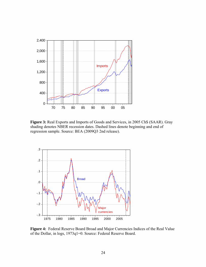
This analysis is inspired by both current events – the widening of the trade deficit

as a proportion of GDP, illustrated in Figure 1 – and recent findings of the persistence of

the Houthakker-Magee results, namely that the income elasticity of U.S. imports exceeds

that of exports. Over the past 30 years, the gap is at least 0.3 for total goods and services,

regardless of the method of estimation. In Chinn (2005), the gap is as high as 0.65. Table

1 presents estimates obtained from OLS, dynamic OLS, single equation error correction

estimates and the Johansen maximum likelihood procedures. Furthermore, there is little

evidence that the asymmetry is disappearing, at least for imports. Breaking the last 30

years into three equal sub-periods, one obtains the income elasticities in Figure 2. In other

words, the asymmetry is proving to be quite durable.

Moreover, the absolute values of the income elasticities are quite high. In Table 1,

the income elasticities are as high as 2.2 for imports, and 1.9 for exports. These large

elasticities are difficult to reconcile with the standard differentiated goods model (see

Goldstein and Khan, 1985). From a forecasting standpoint, high income elasticities1 are

not troubling; but – as discussed below – from an economic perspective, they are

perplexing.2 Finally, the behavior of trade flows during 1999-2000 is difficult to explain

using standard models. As illustrated in Figure 3, both series surge in this period.

In this paper, I re-investigate the behavior of export and import flows, motivating

the analysis by referring to new theories of trade behavior. These include differentiated

1 This phenomenon has been noted before (Rose, 1991). 2 Barrell and Dées (2005) and Camerero and Tamarit (2003) address the issue of very high income elasticities by incorporating FDI. IMF (2007) incorporates exports of intermediates in the import equation, and imports of intermediates in the export equation,

2

goods models such as those forwarded by Krugman (1991). Such approaches do yield

some insights. However, in this paper, I adopt a different approach. Disaggregating the

data, one finds that some of the odd behavior of goods exports and imports can be

isolated to the peculiar behavior of capital goods; since such goods are often used to

manufacture other capital goods or consumer goods, it seems that growth in such

categories is “inflating” the volume of such trade flows. Various papers have pointed out

that the growth of such trade may be nonlinearly related to the decline in trade barriers

and the heightened importance of capital expenditures during certain phases of the

business cycle. More recently, Mann and Plück (2007) have argued that disaggregation

along category line and trading partner helps in obtaining reasonable parameter estimates.

Once one includes the variables that one thinks should matter for such vertical

specialization, the parameter estimates become more plausible. That being said, the

parameter estimates for the auxiliary variables are not always in the expected direction or

statistically significant, and the results cannot be construed as definitive. In addition, the

estimates based upon disaggregated data yield less biased estimates of the long run

equilibrium levels of imports.

2. The Standard Model and the Supply Side

2.1 The model specification

The empirical specification is motivated by the traditional, partial equilibrium view of

trade flows. Goldstein and Khan (1985) provide a clear exposition of this “imperfect

substitutes” model. To set ideas consider the algebraic framework similar to that used by

to account for vertical specialization. This procedure reduces the estimated income

3

Rose (1991). Demand for imports in the US and the Rest-of-the-World (RoW) is given

by:

D f Y PimUS US US

imUS= 1 ( , $ ) (1)

D f Y PimRoW RoW RoW

imRoW= 1 ( , $ ) (2)

where $Pim is the price of imports relative to the economy-wide price level. The supply of

exports is given by:

S f P ZexUS US

exUS US= 2 ( $ , ) (3)

S f P ZexRoW RoW

exRoW RoW= 2 ( $ , ) (4)

Where $Pex is the price of exports relative to the economy-wide price level. Note that the

price of imports into the US is equal to the price of foreign exports adjusted by the real

exchange rate.

$ $ $ $P P E P P P QPimUS US

exRoW RoW

imUS

exRoW× = × × ⇒ = (5)

where E is the nominal exchange rate in US$ per unit of foreign currency, the real

exchange rate is

QEP

P

RoW

US=

where P represents the aggregate level of prices of domestically produced goods and

services. Z is a supply shift variable, representing the productive capacity of the

exportables sector.

An analogous equation applies for imports into the rest-of-the-world. Imposing

the equilibrium conditions that supply equals demand, one can write out import and

elasticities.

4

export equations (assuming log-linear functional forms, where lowercase letters denote

log values of upper case):3

im q y zt t tUS RoW

t= + + + +β β β β ε0 1 2 3 2 (6)

ex q y zt t tRoW US

t= + + + +δ δ δ δ ε0 1 2 3 1 (7)

Where β1 < 0, β2 > 0, β3 > 0 and δ1 > 0, δ2 > 0, δ3 > 0.

Notice that exports are the residual of production over domestic consumption of

exportables; similarly imports are the residual of foreign production over foreign

consumption of tradables. The difference between this specification and the standard is

the inclusion of the exportables supply shift variable, z. In standard import and export

regressions, this term is omitted, implicitly holding the export supply curve fixed; in

other words, it constrains the relationship between domestic consumption of exportables

and production of exportables to be constant (see Helkie and Hooper, 1988 for an

exception to this rule). A bout of consumption at home that reduces the supply available

for exports would induce an apparent structural break in the equation (6) if the z term is

omitted. Similarly, omission of the rest-of-world export suppy term from the import

equation makes the estimated relationships susceptible to structural breaks.

Note that the supply term here is explicitly partial equilibrium in nature. Unlike

the Krugman (1991) model, where balanced trade implies supply creates its own demand,

no specific presumptions are made regarding the source of this supply effect.

3 As Marquez (1994) has pointed out, there are a number of problems with this specification, in terms of assumptions regarding expenditure shares. A number of other potentially important factors are also omitted, including other trend factors (e.g, immigration as in Marquez (2002) or the rise of services exports as in Mann (1999)).

5

The problem, of course, is obtaining good proxies for these supply terms. Obvious

candidates, such as US industrial production for US exports, exhibits too much

collinearity with rest-of-world GDP to identify the supply effect precisely.4 That is why

this supply factor has typically been identified in panel cross section analyses (Bayoumi,

2003; Gagnon, 2004).

2.2 Data and Estimation

Data on real imports and exports and components of real GDP (2005 chain

weighted dollars) were obtained for the 1967q1-2009q3 period. Domestic economic

activity was measured by U.S. GDP in 2005 chain weighted dollars. Foreign economic

activity was measured by real Rest-of-World GDP, weighted by U.S. exports to major

trading partners. The Federal Reserve Board’s broad trade weighted value of the dollar is

used. This index uses the CPI as the deflator.5 (Additional details on all these variables

are contained in Appendix 1.)

Estimation is implemented on data spanning a period of 1975q1-2007q4 (I drop

the period after this in order to omit recession data). This period spans three episodes of

dollar appreciation and three episodes of dollar depreciation; the broad measure of dollar

is used, as opposed to the major currencies measure, which as has been pointed out in

4 In addition, industrial production is in some sense too “endogenous” a variable to include in the regression. An alternative is to obtain capital stock measures as a measure of the supply capacity of exportables, as in Helkie and Hooper (1988). The question is whether these variables are measured with too much error, especially to the extent that we want to capture the impact of the newly industrializing countries and China.

5 For an analysis of how different results are obtained using different deflators, see Chinn (2005). In that analysis, I examine the impact of using alternatively CPI, PPI and unit labor cost deflated real exchange rates. I leave aside the question of whether Divisia indices fully capture the impact of Chinese relative prices. For this question, see Thomas and Marquez (2006).

6

recent reports, is unrepresentative of relative prices faced by the U.S. import competing

sector in recent years (see Figure 4).

The cointegrating relationship is identified using dynamic OLS (Stock and

Watson, 1993). Two leads and four lags of the right hand side variables are included. In a

simple two variable cointegrating relationship, the estimated regression equation is:

y x x ut t ii t i t= + + +=+

−

+∑γ γ0 1 2

4Γ Δ

Although this approach presupposes that there is only one long run relationship, this

requirement is not problematic, as in these extended samples at least one cointegrating

vector is usually detected.

2.3 Empirical Results

First we consider equations (6) and (7) suppressing the z terms. The long run elasticities

are reported in Table 2. The income elasticity for total exports of goods and services is

1.85 (Column [1]). This finding is not an artifact of the inclusion of services. In fact, the

goods only elasticity is 1.92 (Column [3]). The high coefficients hold for different

aggregates including goods ex Agricultural goods, and services.

A similar result obtains for imports. As reported in Table 3, Column [1], total

imports of goods and services also exhibit a long run elasticity of 2.21. The fact that the

estimates are sensitive to the inclusion of a time trend suggests that a cointegrating

relations does not exist between the variables and these very aggregated trade flow

measures.

Consequently, in addition to the empirical motivation for examining different

aggregates, there is a good economic reason to consider, for instance, an import aggregate

7

excluding petroleum. The trade equations in (6) and (7) are derived from an imperfect

substitutes model, well suited to manufactured goods. However, oil is a natural resource

commodity that does not quickly respond to market signals, and exhibits trends due to

resource depletion. A related argument might be used to motivate a focus on a non-

agricultural goods export variable.

Interestingly, these remarkably high estimated income elasticity estimates persist,

for both export goods ex Agriculture and import goods ex oil (columns [3] in Tables 2

and 3). On the other hand, estimated price elasticities are higher (in absolute value).

These high estimated income elasticities inform the debate over the durability of

the Houthakker-Magee (1969) findings. Exports involving goods respond 1.9 percent for

each one percentage point increase in rest-of-world income. In contrast, imports rise

about 2.2 to 3.0 percentage points for each percentage point increase in US GDP. This set

of findings suggests that the Houthakker-Magee income asymmetry persists. Hence, even

if U.S. and foreign growth rates were to converge, net exports would continue to

deteriorate even starting from balanced trade. Obviously, starting from an initial trade

deficit, the trend deterioration would be even more pronounced.

All of the preceding specifications exclude a role for the supply side, suggested by

Equations (6) and (7). As noted earlier, it is hard to find good measures of the supply

side. Helkie and Hooper (1988) used a measure of relative capital stock, but it is hard to

think of how one would accurately estimate the relevant rest of the world capital stock,

especially with the entry of China.

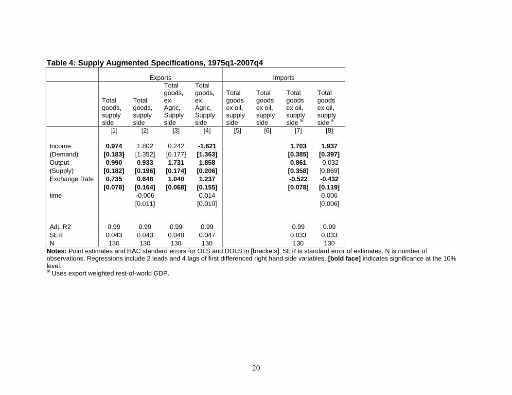
For exports of goods, accounting for supply is fairly successful. In Table 4, when

U.S. manufacturing industrial production is included, the export income elasticity falls

8

from 1.9 to 1.0, with the supply coefficient equal to close to unity (Column [1]).

Interestingly, the results are not sensitive to the inclusion of a time trend. Counter-

intuitively, exports of goods ex Agriculture are not as easily modeled. Inclusion of a time

trend leads to a negative coefficient estimate on real GDP.

On the import side, the inclusion of supply side effects is slightly more

successful. In this case, the supply side variable is import-weighted real GDP. In Table 4,

Column [5], the import income elasticity falls to 2.60 from 1.70, with the coefficient on

foreign GDP equal to 0.861.

Unfortunately, in all these instances, the demand and supply variables are so

collinear that the results are sensitive to the inclusion of the time trends.6 This is why

cross-section and panel regressions such as Gagnon (2003) and Bayoumi (2003) obtain

more supportive evidence of supply side effects.

3. Vertical Specialization and Tariffs

One hint of why the income elasticities are so large is provided by the surge in both

exports and imports during 1999-2000. In informal discussions, this jump is associated

with the investment boom; the category experiencing the largest jump is capital goods.

The fact that the surge and collapse occurred in both categories could be

coincidence – evidence of a synchronized worldwide investment boom. Or it could be a

reflection that the two are interlinked.

Recent research has focused on the rise of intermediate goods in international

trade. However, intermediate goods are not in and of themselves sufficient to explain the

9

rise in trade. It is intermediate goods trade used to produce other traded goods – in other

words vertical specialization (Hummels, et al., 2001; Yi, 2003; Chen et al., 2005) – that is

required. This process of importing in order to export has also been termed the

“fragmentation” of the production process (Arndt, 1997). At this juncture, it is useful to

recognize that services exhibit less of this fragmentation. This explains in part the

differential import income elasticities: 2.62 for goods ex oil versus 1.64 for services.7

Table 5 estimates the basic regressions specification (trade flow on income and

real exchange rate) for the trade flow ex capital goods and capital goods trade flows. For

the specifications excluding a time trend, goods exports ex capital goods (Column [1])

exhibit an income elasticity of 1.17 while capital goods exports (Column [3]) exhibit an

elasticity of 2.86. For imports, this pattern is repeated, but more sharply. The income

elasticity for total goods imports ex oil and capital goods is 1.97, while that for capital

goods is nearly 4.61, for specifications excluding time trends (Columns [5] and [7]). In

both cases, the trend-augmented specifications exhibit a similar, although less

pronounced, pattern.

These findings suggest two not necessarily inconsistent conclusions. First, that it

is important to disaggregate goods exports and imports in order to model aggregate trade

flows. Second, if one is to model aggregate goods flows, one needs to include the

measures that have a specific impact on the capital goods portions.

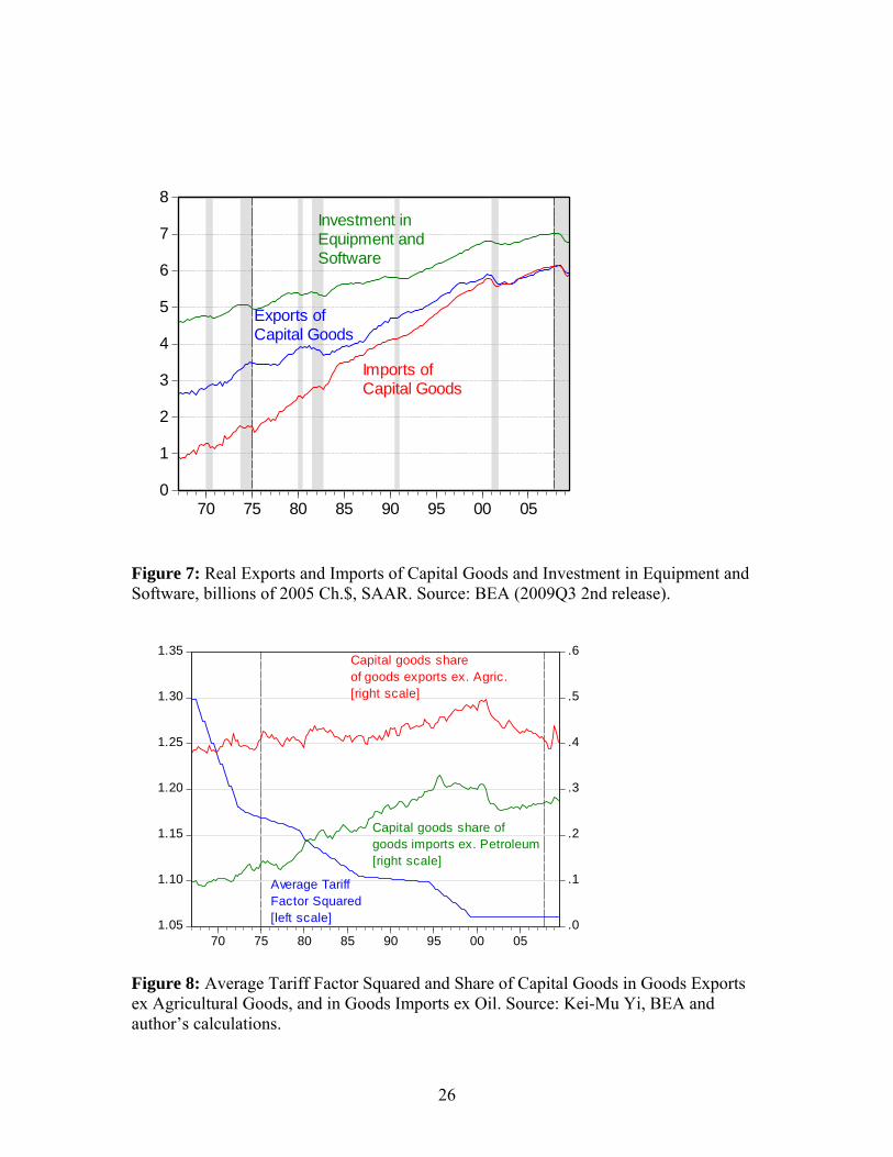
Figures 5 and 6 show how differently different goods aggregates behave. Note

that the series excluding capital goods exhibits much less of a pronounced hump. Figure

6 For a survey of research related to the ongoing trade collapse and rebound, see Baldwin (2009). Freund (2009) provides empirical evidence over time.

10

7 illustrates how capital goods exports and imports covary with investment in equipment

and software, particularly in the 1999-2001 period. The importance of vertical

specialization was suggested, particularly for hi-tech goods, in analyses around the time

of the capital goods surges (e.g., Council of Economic Advisers, 2001, Chapter 4).

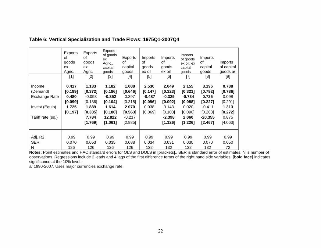
The regression results in Column [1] of Table 6 indicate the impact of export-

weighted Rest-of-World investment in equipment and software on total goods exports:

income now has a less than elastic impact, while investment has an elasticity of 1.70. Yi

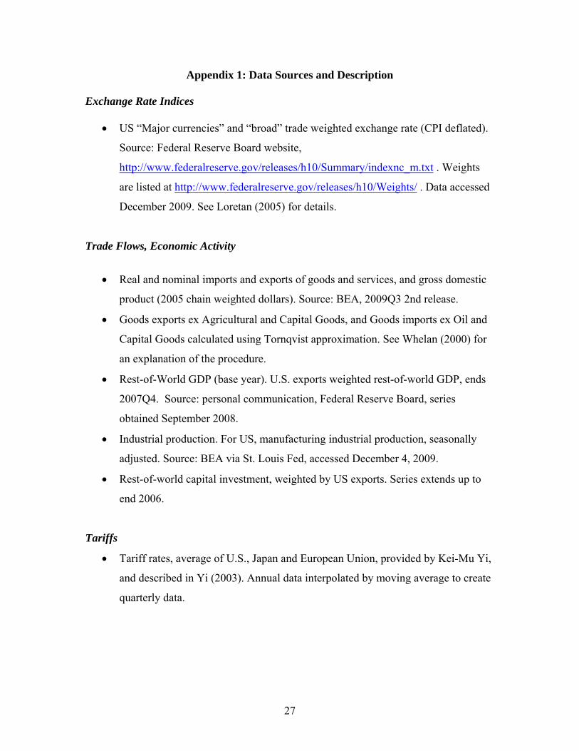
(2003) argues that reductions in the tariff rate have induced large, non-proportionate,

changes in the extent of vertical specialization. To incorporate this factor, I augment the

regression with the (square of the) average tariff rate of the US, Europe and Japan.8 This

variable does not enter with the correct sign for goods exports ex Agricultural goods, or

ex Agricultural and Capital goods (Columns [2] and [3]).

When examining capital goods exports (Column [4]), the income elasticity is

slightly above unity and the price elasticity is 0.4 (albeit not significant). Investment

again enters in with a high elasticity, while squared tariff rate does not enter with a

statistically significant coefficient.

Examining non-oil goods imports in a specification augmented in by investment

(Column [5]) yields a relatively high income elasticity of 2.53. Investment is not

statistically significant. Augmenting the specification with the tariff rate squared

(Column [6]) yields a statistically significant coefficient on this variable, in the expected

direction, while raising the investment coefficient. This is suggestive that the decline in

7 Marquez (2005) obtains similar estimates, but points out that further disaggregation of services leads to different insights on income and price elasticities.

11

G-3 tariff rates and the rise in investment are correlated. In addition the income

coefficient declines to 2.0; most likely income was picking up the trend in the tariff

variable in the standard specifications. Non-oil, non-capital goods imports (Column [7])

show a minor effect from investment and a wrong-signed effect from tariffs.

In contrast, imports of capital goods (Columns [8]) exhibit a strong

responsiveness to income and tariff rates. Exchange rates exhibit wrong signedness and

equipment and software expenditures are not statistically significant.

The results for capital goods imports are sensitive to the specific time sample.

Restricting the sample to 1990-2007 yields the results in column [9]. Estimated

coefficients on income and investment are statistically significant, while those on tariffs

and the exchange rate are not. The absence of strong effects could be due to the lower

variability of these variables during the later time period. On the other hand, one

advantage of a shorter sample period is that the standard error of regression shrinks from

0.070 to 0.050.

4. Summary

In this paper the data for U.S. trade flows up to end of 2006 are investigated. The results

indicate. A variety of different aggregates are examined. In addition, supply side factors

and the implications of vertical specialization are accounted for. A number of conclusions

are derived from this assessment.

8 Of course, this is a narrow definition of trade costs. For a broader interpretation, see Jacks, Meissner and Novy (2009).

12

First, the examination confirms that the Houthakker-Magee finding of income

asymmetries persists into the most recent period. This characterization applies most

strongly to specifications involving highly aggregated trade flows, and no role for supply

or other factors.

Second, the disaggregation of trade flows into services and some subcategory of

goods usually yields higher estimated price elasticities. This outcome suggests some role

for aggregation bias in driving down estimated price elasticities. A similar finding was

obtained in the recent IMF study, but in that case, the results pertained to price elasticities

for relative prices, instead of the real exchange rate as in this study.

Third, the inclusion of supply-side variables reduces the magnitude of income

elasticities for goods. However, the results are not robust to the inclusion of time trends.

Consequently, one can only make tentative conclusions regarding the importance of

supply side factors in driving the increasing volume of international trade. On the other

hand, cross-section studies of trade do suggest that the finding of a supply side role is not

completely coincidental.

Fourth, capital goods and non-capital goods imports appear to behave differently.

Capital goods exports respond strongly to investment in equipment and software.

Depending upon the sample period, capital goods imports respond strongly to the tariff

rate or investment. However, because the results are sensitive to the sample period and

trade flow measure, additional work is required to identify the channels by which trade

barriers and vertical specialization interact. In particular, one might want a better measure

of trade barriers for trade in capital goods.

13

Finally, it appears that disaggregation – even of a limited extent – might prove

helpful in improving predictions of aggregate trade flows. One key dividing line appears

to be between non-oil non-capital goods and capital goods. 9

9 In previous versions of this paper, I’ve reported results that indicate that sums of predicted import sub-aggregates appear to yield smaller prediction errors than using a predicted aggregate import variable. This finding – while not definitive – suggests that one can improve our forecasts of trade flows without resorting to modeling many very highly disaggregated trade series.

14

References

Baldwin, Richard (editor), 2009, The Great Trade Collapse: Causes, Consequences and Prospects (London: CEPR). Barrell, Ray and Stephane Dées, 2005, “World Trade and Global Integration in Production Processes: A Re-assessment of Import Demand Equations,” ECB Working Paper No. 503 (Frankfurt: European Central Bank, July). Bayoumi, Tamim, 2003, “Estimating Trade Equations from Aggregate Bilateral Data,” mimeo (Washington, D.C.: IMF, December). Bayoumi, Tamim, Jaewoo Lee, and Sarma Jayantha, 2005, “New Rates from New Weights,” Working Paper No. WP/05/99 (Washington, DC: IMF, May). Camarero, Mariam and Cecilio Tamarit, 2003, “Estimating the export and import demand for manufactured goods: The role of FDI,” Leverhulme Center Research Paper Series No. 2003/34 (Nottingham: University of Nottingham). Chen, Hogan, Matthew Kondratowicz and Kei-Mu Yi, 2005, “Vertical Specialization and Three Facts about U.S. International Trade,” North American Journal of Economics and Finance 16: 35–59 Chinn, Menzie D., 2005, “Doomed to Deficits? Aggregate U.S. Trade Flows Re-examined,” Review of World Economics 141(3): 460-85. Revision of NBER Working Paper No. 9521 (February 2003). Council of Economic Advisers, 2001, Economic Report of the President, 2001 (Washington, D.C.: U.S. GPO, January). Freund, Caroline, 2009, “The Trade Response to Global Downturns: Historical Evidence,” Policy Research Working Paper No. 5015 (Washington, D.C.: World Bank, August). Gagnon, Joseph E., 2003, “Productive Capacity, Product Varieties, and the Elasticities Approach to the Trade Balance,” International Finance and Discussion Papers No. 781 (October). Goldstein, Morris, and Mohsin Khan, 1985, Income and Price Effects in Foreign Trade, in R. Jones and P. Kenen (eds.), Handbook of International Economics, Vol. 2, (Amsterdam: Elsevier).

15

Helkie, William and Peter Hooper, 1988, “The U.S. External Deficit in the 1980’s: An Empirical Analysis,” in R. Bryant, G. Holtham and P. Hooper (eds.) External Deficits and the Dollar: The Pit and the Pendulum. Washington, DC: Brookings Institution. Hooper, Peter, Karen Johnson and Jaime Marquez, 2000, Princeton Studies in International Economics No. 87 (Princeton, NJ: Princeton University). Houthakker, Hendrik, and Stephen Magee, 1969, Income and Price Elasticities in World Trade, Review of Economics and Statistics 51: 111-25. Hummels, David, Jun Ishii, and Kei-Mu Yi, 2001, “The Nature and Growth of Vertical Specialization in World Trade,” Journal of International Economics 54: 75-96. IMF, 2007, World Economic Outlook (IMF: Washington, D.C., April). Jacks, David, Christopher Meissner and Dennis Novy, 2009, “Trade Booms, Trade Busts, and Trade Costs,” mimeo (August 2009). Johansen, Søren, 1988, Statistical Analysis of Cointegrating Vectors. Journal of Economic Dynamics and Control 12: 231-54. Johansen, Søren, and Katerina Juselius, 1990, Maximum Likelihood Estimation and Inference on Cointegration - With Applications to the Demand for Money. Oxford Bulletin of Economics and Statistics 52: 169-210. Lawrence, Robert Z., 1990, “U.S. Current Account Adjustment: An Appraisal,” Brookings Papers on Economic Activity No. 2: 343-382. Leahy, Michael P., 1998, New Summary Measures of the Foreign Exchange Value of the Dollar. Federal Reserve Bulletin (October): 811-818. Loretan, Mico, 2005, “Indexes of the Foreign Exchange Value of the Dollar,” Federal Reserve Bulletin (Winter): 1-8. Mann, Catherine, 1999, Is the U.S. Trade Deficit Sustainable (Washington, DC: Institute for International Economics). Mann, Catherine, and Katharina Plück, 2007, “The U.S. Trade Deficit: A Disaggregated Perspective,” in Richard Clarida (ed.), G7 Current Account Imbalances: Sustainability and Adjustment (U.Chicago Press). Marquez, Jaime, 2005, “Estimating Elasticities for U.S. Trade in Services,” International Finance Discussion Papers No. 836. Washington, D.C.: Board of Governors of the Federal Reserve System, August.

16

Marquez, Jaime, 2002, Estimating Trade Elasticities, Advanced Studies in Theoretical and Applied Econometrics, Vol. 39 (Boston; Dordrecht and London: Kluwer Academic). Marquez, Jaime, 1994, “The Econometrics of Elasticities or the Elasticity of Econometrics: An Empirical Analysis of the Behavior of U.S. Imports,” Review of Economics and Statistics 76(3) (August): 471-481. Meade, Ellen, 1991, “Computers and the Trade Deficit: the case of the falling prices,” in Peter Hooper and David Richardson, (eds.) International Economic Transactions: Issues in Measurement and Empirical Research, NBER Studies in Income and Wealth vol. 55. Stock, James H. and Mark W. Watson, 1993, “A Simple Estimator of Cointegrating Vectors in Higher Order Integrated Systems,” Econometrica 61(4): 783-820. Thomas, Charles P. and Jaime Marquez, 2006, “Measurement Matters for Modeling U.S. Import Prices,” International Finance and Discussion Papers 2006-863 (Washington, D.C.: Federal Reserve Board, December). Whelan, Karl, 2000, “A Guide to the Use of Chain Aggregated NIPA Data,” Finance and Economics Discussion Papers No. 2000-35 (Washington, DC: Board of Governors of the Federal Reserve System). Yi, Kei-Mu, 2003, “Can Vertical Specialization Explain the Growth of World Trade?” Journal of Political Economy 111(1): 53-102.

17

Table 1: Estimates of Export and Import Elasticities, 1975q1-2007q4

Exports of Goods and Services

Imports of Goods and Services

OLS DOLS a/ ECM b/ VECM OLS DOLS a/ ECM b/ VECM [1] [2] [3] [4] [5] [6] [7] [8]

Income 1.834 1.853 1.882 1.887 2.200 2.193 2.205 2.227 (Demand) [0.037] [0.033] [0.055] [0.046] [0.034] [0.030] [0.068] [0.038] Exchange rate 0.471 0.595 0.955 0.835 -0.162 -0.238 -0.259 -0.162 [0.079] [0.085] [0.209] [0.178] [0.071] [0.082] [0.164] [0.126] Adj. R2 0.99 0.99 0.37 Na 0.99 0.99 0.34 Na SER 0.063 0.050 0.018 Na 0.056 0.048 0.023 Na N 132 130 132 132 128 132 132 132 Coint. Vectors Na na 1 0,0 na na 1 0,1

Notes: Point estimates and HAC standard errors for OLS and DOLS in [brackets], implied long run coefficients from ECM and cointegrating vector coefficients for VECM [asymptotic standard errors in brackets]. SER is standard error of estimates. N is number of observations. Cointegrating vectors is the number of indicated cointegrating vectors; under VECM, {#,#} indicates the number of vectors as indicated by the trace and maximal eigenvalue statistics at the 5% level, using the asymptotic critical values. [bold face] indicates significance at the 10% level. a/ Includes 2 leads and 4 lags of the first differenced right hand side variables. b/ Includes 3 lags of the first differenced right hand side variables.

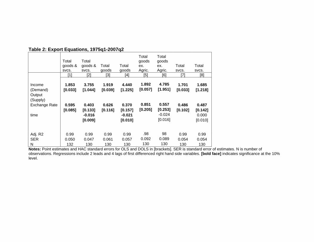
Table 2: Export Equations, 1975q1-2007q2

Total goods & svcs.

Total goods & svcs.

Total goods

Total goods

Total goods ex. Agric.

Total goods ex. Agric.

Total svcs.

Total svcs.

[1] [2] [3] [4] [5] [6] [7] [8] Income 1.853 3.755 1.919 4.440 1.892 4.785 1.701 1.685 (Demand) [0.033] [1.044] [0.039] [1.225] [0.057] [1.951] [0.033] [1.218] Output (Supply) Exchange Rate 0.595 0.403 0.626 0.370 0.851 0.557 0.486 0.487 [0.085] [0.133] [0.116] [0.157] [0.205] [0.253] [0.102] [0.142] time -0.016 -0.021 -0.024 0.000 [0.009] [0.010] [0.016] [0.010] Adj. R2 0.99 0.99 0.99 0.99 .98 98 0.99 0.99 SER 0.050 0.047 0.061 0.057 0.092 0.089 0.054 0.054 N 132 130 130 130 130 130 130 130

Notes: Point estimates and HAC standard errors for OLS and DOLS in [brackets]. SER is standard error of estimates. N is number of observations. Regressions include 2 leads and 4 lags of first differenced right hand side variables. [bold face] indicates significance at the 10% level.

19

Table 3: Import Equations, 1975q1-2007q4

Total goods & svcs.

Total goods & svcs.

Total goods

Total goods

Total goods ex oil

Total goods ex oil

Total svcs.

Total svcs.

[1] [2] [3] [4] [5] [6] [7] [8] Income 2.194 3.000 2.313 3.203 2.623 2.033 1.641 1.354 (Demand) [0.030] [0.387] [0.038] [0.512] [0.016] [0.310] [0.028] [0.487] Output (Supply) Exchange Rate -0.133 -0.127 -0.096 -0.089 -0.404 -0.408 -0.293 -0.295 [0.085] [0.068] [0.115] [0.095] [0.075] [0.070] [0.109] [0.107] time -0.006 -0.008 0.005 0.002 [0.003] [0.004] [0.002] [0.004] Adj. R2 0.99 0.99 0.99 0.99 0.99 0.99 0.99 0.99 SER 0.047 0.045 0.062 0.059 0.035 0.033 0.057 0.057 N 132 132 132 132 132 132 132 132

Notes: Point estimates and HAC standard errors for OLS and DOLS in [brackets]. SER is standard error of estimates. N is number of observations. Regressions include 2 leads and 4 lags of first differenced right hand side variables. [bold face] indicates significance at the 10% level.

20

Table 4: Supply Augmented Specifications, 1975q1-2007q4

Exports Imports

Total goods, supply side

Total goods, supply side

Total goods, ex. Agric, Supply side

Total goods, ex. Agric, Supply side

Total goods ex oil, supply side

Total goods ex oil, supply side

Total goods ex oil, supply side a/

Total goods ex oil, supply side a/

[1] [2] [3] [4] [5] [6] [7] [8] Income 0.974 1.802 0.242 -1.621 1.703 1.937 (Demand) [0.183] [1.352] [0.177] [1.363] [0.385] [0.397] Output 0.990 0.933 1.731 1.858 0.861 -0.032 (Supply) [0.182] [0.196] [0.174] [0.206] [0.358] [0.869] Exchange Rate 0.735 0.648 1.040 1.237 -0.522 -0.432 [0.078] [0.164] [0.068] [0.155] [0.078] [0.119] time -0.006 0.014 0.006 [0.011] [0.010] [0.006] Adj. R2 0.99 0.99 0.99 0.99 0.99 0.99 SER 0.043 0.043 0.048 0.047 0.033 0.033 N 130 130 130 130 130 130

Notes: Point estimates and HAC standard errors for OLS and DOLS in [brackets]. SER is standard error of estimates. N is number of observations. Regressions include 2 leads and 4 lags of first differenced right hand side variables. [bold face] indicates significance at the 10% level. a/ Uses export weighted rest-of-world GDP.

21

Table 5: Capital Goods versus Non-Capital Goods Trade Flows, 1975q1-2009q3

Exports Imports

Total goods ex Agric., capital goods

Total goods ex Agric., capital goods

Capital goods

Capital goods

Total goods ex oil, capital goods

Total goods ex oil, capital goods

Capital goods

Capital goods

[1] [2] [3] [4] [5] [6] [7] [8] Income 1.172 3.283 2.855 6.649 1.970 1.584 4.610 1.684 (Demand) [0.059] [1.943] [0.081] [2.530] [0.020] [0.255] [0.126] [1.413] Exchange Rate 0.854 0.640 0.874 0.490 -0.536 -0.538 -0.180 -0.202 [0.221] [0.263] [0.220] [0.329] [0.045] [0.046] [0.416] [0.365] time -0.018 -0.032 0.003 0.023 [0.016] [0.021] [0.002] [0.011] Adj. R2 0.93 0.94 0.98 0.98 0.99 0.99 0.99 0.99 SER 0.096 0.095 0.118 0.114 0.033 0.032 0.178 0.171 N 130 130 130 130 132 132 132 132

Notes: Point estimates and HAC standard errors for OLS and DOLS in [brackets]. SER is standard error of estimates. N is number of observations. Regressions include 2 leads and 4 lags of the first difference terms of the right hand side variables. [bold face] indicates significance at the 10% level.

22

Table 6: Vertical Specialization and Trade Flows: 1975Q1-2007Q4

Exports of goods ex. Agric.

Exports of goods ex. Agric

Exports of goods ex Agric., capital goods

Exports of capital goods

Imports of goods ex oil

Imports of goods ex oil

Imports of goods ex oil, ex capital goods

Imports of capital goods

Imports of capital goods a/

[1] [2] [3] [4] [5] [6] [7] [8] [9] Income 0.417 1.133 1.182 1.088 2.530 2.049 2.155 3.196 0.788 (Demand) [0.189] [0.372] [0.186] [0.646] [0.147] [0.323] [0.321] [0.792] [0.786] Exchange Rate 0.480 -0.098 -0.352 0.397 -0.487 -0.329 -0.734 0.725 0.098 [0.099] [0.186] [0.104] [0.318] [0.096] [0.092] [0.088] [0.227] [0.291] Invest (Equip) 1.725 1.889 1.614 2.070 0.038 0.143 0.020 -0.411 1.313 [0.197] [0.335] [0.180] [0.563] [0.069] [0.103] [0.090] [0.268] [0.272] Tariff rate (sq.) 7.784 12.822 -0.217 -2.398 2.060 -20.355 0.875 [1.769] [1.061] [2.985] [1.126] [1.226] [2.467] [4.063] Adj. R2 0.99 0.99 0.99 0.99 0.99 0.99 0.99 0.99 0.99 SER 0.070 0.053 0.035 0.088 0.034 0.031 0.030 0.070 0.050 N 126 126 126 126 132 132 132 132 72

Notes: Point estimates and HAC standard errors for OLS and DOLS in [brackets].. SER is standard error of estimates. N is number of observations. Regressions include 2 leads and 4 lags of the first difference terms of the right hand side variables. [bold face] indicates significance at the 10% level. a/ 1990-2007. Uses major currencies exchange rate.

-.07

-.06

-.05

-.04

-.03

-.02

-.01

.00

.01

.02

70 75 80 85 90 95 00 05

Net exportsto GDP ratio

Figure 1: Net Exports of goods and services to GDP ratio, SAAR. Shaded areas denote recession dates. Source: BEA (April 2007 release) and NBER for recession dates.

0.0

0.5

1.0

1.5

2.0

2.5

3.0

EXPY IMPY

1975-85 1986-96 1997-2006

Exports,1975-2007

Imports,1975-2007

Figure 2: Income Export (EXPY) and Import (IMPY) Elasticities for Subperiods. Source: Columns [2] and [6] from Table1, and DOLS regressions on the indicated subperiod.

24

0

400

800

1,200

1,600

2,000

2,400

70 75 80 85 90 95 00 05

Exports

Imports

Figure 3: Real Exports and Imports of Goods and Services, in 2005 Ch$ (SAAR). Gray shading denotes NBER recession dates. Dashed lines denote beginning and end of regression sample. Source: BEA (2009Q3 2nd release).

-.3

-.2

-.1

.0

.1

.2

.3

1975 1980 1985 1990 1995 2000 2005

Broad

Majorcurrencies

Figure 4: Federal Reserve Board Broad and Major Currencies Indices of the Real Value of the Dollar, in logs, 1973q1=0. Source: Federal Reserve Board.

25

4.4

4.8

5.2

5.6

6.0

6.4

6.8

7.2

70 75 80 85 90 95 00 05

Exportsof Goods

Ex. Agric.

Ex. Agric.,CapitalGoods

Figure 5: Log Real Exports of Goods, Goods ex Agricultural Goods, Goods ex Agricultural and Capital Goods, billions of 2005 Ch.$, SAAR. Source: BEA (2009Q3 2nd release), and author’s calculations.

4.0

4.5

5.0

5.5

6.0

6.5

7.0

7.5

8.0

70 75 80 85 90 95 00 05

Importsof Goods

Ex. Petroleum

Ex. Petroleum,Capital Goods

Figure 6: Log Real Imports of Goods, Goods ex Petroleum, and Goods ex Petroleum and Capital Goods, billions of 2005 Ch.$, SAAR. Source: BEA (2009Q3 2nd release), and author’s calculations.

26

0

1

2

3

4

5

6

7

8

70 75 80 85 90 95 00 05

Exports ofCapital Goods

Imports ofCapital Goods

Investment inEquipment andSoftware

Figure 7: Real Exports and Imports of Capital Goods and Investment in Equipment and Software, billions of 2005 Ch.$, SAAR. Source: BEA (2009Q3 2nd release).

1.05

1.10

1.15

1.20

1.25

1.30

1.35

.0

.1

.2

.3

.4

.5

.6

70 75 80 85 90 95 00 05

Average TariffFactor Squared[left scale]

Capital goods shareof goods exports ex. Agric.[right scale]

Capital goods share ofgoods imports ex. Petroleum[right scale]

Figure 8: Average Tariff Factor Squared and Share of Capital Goods in Goods Exports ex Agricultural Goods, and in Goods Imports ex Oil. Source: Kei-Mu Yi, BEA and author’s calculations.

27

Appendix 1: Data Sources and Description

Exchange Rate Indices

• US “Major currencies” and “broad” trade weighted exchange rate (CPI deflated).

Source: Federal Reserve Board website,

http://www.federalreserve.gov/releases/h10/Summary/indexnc_m.txt . Weights

are listed at http://www.federalreserve.gov/releases/h10/Weights/ . Data accessed

December 2009. See Loretan (2005) for details.

Trade Flows, Economic Activity

• Real and nominal imports and exports of goods and services, and gross domestic

product (2005 chain weighted dollars). Source: BEA, 2009Q3 2nd release.

• Goods exports ex Agricultural and Capital Goods, and Goods imports ex Oil and

Capital Goods calculated using Tornqvist approximation. See Whelan (2000) for

an explanation of the procedure.

• Rest-of-World GDP (base year). U.S. exports weighted rest-of-world GDP, ends

2007Q4. Source: personal communication, Federal Reserve Board, series

obtained September 2008.

• Industrial production. For US, manufacturing industrial production, seasonally

adjusted. Source: BEA via St. Louis Fed, accessed December 4, 2009.

• Rest-of-world capital investment, weighted by US exports. Series extends up to

end 2006.

Tariffs

• Tariff rates, average of U.S., Japan and European Union, provided by Kei-Mu Yi,

and described in Yi (2003). Annual data interpolated by moving average to create

quarterly data.