Robert L. Ehrlich, Jr., Governor Secretary · Tests of total suspended solids, total ... Appendix...
84
STATE HIGHWAY ADMINISTRATION RESEARCH REPORT Polyacrylamide use for Sediment Reduction in Construction Site Stormwater SP508B4J FINAL REPORT September 2006 MD-06-SP508B4J Robert L. Ehrlich, Jr., Governor Michael S. Steele, Lt. Governor Robert L. Flanagan, Secretary Neil J. Pedersen, Administrator Department of Civil and Environmental Engineering University of Maryland College Park, MD 20742 Allen P. Davis, Ph.D., P.E. , Matthew D. Hafner
Transcript of Robert L. Ehrlich, Jr., Governor Secretary · Tests of total suspended solids, total ... Appendix...

STATE HIGHWAY ADMINISTRATION
RESEARCH REPORT
Polyacrylamide use for Sediment Reduction in Construction Site Stormwater
SP508B4J FINAL REPORT
September 2006
MD-06-SP508B4J
Robert L. Ehrlich, Jr., Governor Michael S. Steele, Lt. Governor
Robert L. Flanagan, Secretary Neil J. Pedersen, Administrator
Department of Civil and Environmental Engineering University of Maryland College Park, MD 20742
Allen P. Davis, Ph.D., P.E. , Matthew D. Hafner

The contents of this report reflect the views of the author who is responsible for the fact
sand the accuracy of the data presented herein. The contents do not necessarily reflect the official views or policies of the Maryland State Highway Administration. This report does not constitute a standard, specification, or regulation.

Technical Report Documentation Page
1. Report No.
4. Title & Subtitle Polyacrylamide use for Sediment Reduction in Construction Site Stormwater
5. Report Date September 2006
6. Performing Organization Code
7. Author/s Allen P. Davis, Matthew D. Hafner
8. Performing Org. Report No.
9. Performing Organization Name and Address Department of Civil and Environmental Engineering University of Maryland College Park, MD 20742
10. Work Unit No. (TRAIS)
11. Contract or Grant No. SP508B4J 13. Type of Report and Period Covered Final Report
12. Sponsoring Organization Name and Address Maryland State Highway Administration Office of Policy & Research 707 N. Calvert Street Baltimore, MD 21202
14. Sponsoring Agency Code
15. Supplementary Notes 16. Abstract Sedimentation basins are used to collect runoff from construction sites and reduce the amount of sediment transported to local water bodies. Chemical coagulants are used to increase sedimentation efficiency rates in a variety of water and wastewater treatment processes. Laboratory studies were conducted using anionic and cationic polyacrylamides as well as alum to evaluate efficiency on sediment pond performance. Tests of total suspended solids, total solids, and turbidity were conducted. Laboratory studies of various coagulants demonstrated the potential to reduce turbidity by an additional 25-35%. A protocol was developed for the selection of proper coagulants for field testing. 17. Key Words Stormwater, Sedimentation Basin, Coagulant, Polyacrylamide, Alum
18. Distribution Statement This document is available from the Research Division upon request.
19. Security Classification (of this report) None
20. Security Classification (of this page) None
21. No of pages 77
22. Price N/A
MD-06-SP508B4J 2. Government Accession No 3. Recipient’s Catalog No.
Form DOT F1700.7 (8-72) Reproduction of form and completed page is authorized.

Table of Contents Executive Summary i Introduction and Background 1 Literature Review 3 Methodology 11 Results 17 Analysis 23 Field Testing 25 Conclusions and Recommendations for Implementation 28 References 29 Appendix Figures 32 Appendix Protocol 76 Tables and Figures Table 1. Polymer Characteristics 12 Table 2. Basin Characteristics 13 Table 3. Results of Coagulant Comparison Lab Trials 22 Figure 1. Photos of Site Basins at Construction Site, Rt. 43, Baltimore, Co. 2 Figure 2. Anionic polyacrylamide 4 Figure 3. Field Implementation Schematic for coagulant-assisted sediment basins 26 Appendix Figure 1. May 5 Field Test 32 Appendix Figure 2. June 3 Field Test 33 Appendix Figure 3. N-300 Lab Test 34 Appendix Figure 4. A-110 Lab Test 36 Appendix Figure 5. A-120 Lab Test 38 Appendix Figure 6. A-100 Lab Test 40 Appendix Figure 7. A-130 Lab Test 42 Appendix Figure 8. A-150 Lab Test 1 44 Appendix Figure 9. A-150 Lab Test 2 46 Appendix Figure 10. alum Lab Test 1 48 Appendix Figure 11. alum Lab Test 2 50 Appendix Figure 12. A-130V Lab Test 52 Appendix Figure 13. C-446 Lab Test 54 Appendix Figure 14. C-496 Lab Test 56 Appendix Figure 15. C-448 Lab Test 58 Appendix Figure 16. C-498 Lab Test 60 Appendix Figure 17. Ratios 62 Appendix Figure 18. Comparison Lab Trial 1 63 Appendix Figure 19. Comparison Lab Trial 2 65 Appendix Figure 20. Comparison Lab Trial 3 67 Appendix Figure 21. Comparison Lab Trial 4 69 Appendix Figure 22. pH Study 71 Appendix Figure 23. Width vs. Slope Channel Design 75

Executive Summary
Sedimentation basins are used at all Maryland State Highway Administration (SHA)
construction sites to reduce runoff sediment transport into local water bodies. During storm
events, these ponds can have reduced efficiency, causing very turbid water to exit the basin.
Chemical coagulants are used in various water and wastewater treatments to reduce turbidity and
suspended solids concentrations. Recently coagulants have been used in other states to reduce
runoff sediment at construction sites. The potential for increased water quality using coagulants
has been documented as conditional to the sediment characteristics. Coagulant studies of local
sediments have not been conducted.
This project evaluates the performance of coagulants for sediment reduction in
construction site runoff in a laboratory setting. The two major objectives of this study were to
assess the performance of polymers for sediment reduction and to develop a protocol to be used
for future coagulant selection
A test site was selected at MD 43 in Baltimore County. The MD 43 site consisted of four
sedimentation basins. Stormwater runoff from the Rt. 43 site was collected on several occasions.
Several anionic and cationic polyacrylamides of various doses were added to the samples and
tested for total suspended solids, total solids, and turbidity over time. Alum was also tested as a
coagulant. The efficiency of the anionic and cationic polyacrylamides and alum were compared
using percent removal and turbidity ratios. Comparison trials using the top performing
coagulants for this site were conducted to accurately assess the best coagulant for use in future
field trials.
Overall, twelve different coagulants were tested using the stormwater from the MD 43
basins. Turbidity and percent removal ratios were calculated from laboratory data of the

individual coagulants at the most effective dosage. These ratios were then used to select the best
of the coagulants, A-100, A-110, C-448, (all from Cytec Industries) and alum were chosen for
further comparison trials. A-100 and A-110 are anionic polyacrylamides and C-448 is a cationic
polyacrylamide.
In the comparison trials, all coagulants performed better in all tests than the samples
without coagulant addition.
Coagulant Dose (mg/L)
Average % removal TSS
Average % removal TS
Average % reduction turbidity
No coagulant None 88 68 51 A-100 2 96 76 78 A-110 2 95 76 72 C-448 6 97 76 85 Alum 100 97 78 84
Alum and the cationic polyacrylamide C-448 performed the best in the comparison trials.
However, because cationic polyacrylamide is a known toxin to aquatic organisms, it is not
recommended for field testing. Field testing is recommended for future studies as the proper
coagulant can vary based on site characteristics. This study demonstrates the potential for
coagulant use in construction site sedimentation basins.
Field testing was an initial goal of the project, but it became evident that much laboratory
testing was needed before field testing could be effective. However, a field testing protocol and
implementation process was developed through laboratory and literature research. The protocol
assists in choosing the proper coagulant for the sediment type and the process for implementation
is presented with the materials and methods required.
This study provides important information to SHA about the potential for coagulant-
assisted stormwater basins for active road construction sites. Laboratory data demonstrated the
effectiveness of several coagulants for this use. The additional removal of suspended solids and
ii

turbidity can greatly reduce the pollution entering the local waters of active construction sites.
Continued field research into the implementation of coagulant-assisted stormwater basins will
provide additional data into the feasibility of this option as a pollution prevention method.
iii

Introduction and Background
Increasing concern for the Chesapeake Bay and its tributaries, some of which are water
supplies, have prompted a greater focus on technologies to reduce pollutant inputs to these water
bodies. Some of the greatest challenges are related to addressing nonpoint sources of pollutants.
As a result of highway construction and operation practices, the characteristics of the land
surface are typically altered. The Maryland State Highway Administration (SHA) has been
proactive in developing and implementing technologies to reduce environmental impacts of
highway-related projects. One current concern for SHA projects is stormwater discharges of
sediments.
During the construction of new highways, often vast expanses of soil are exposed to the
elements. After heavy rains, significant erosion potential exists on the sites. To protect local
streams from receiving the sediment, sedimentation basins are constructed to collect the runoff.
These basins allow the sediment in the runoff to settle before the water is drained to the natural
waterbody. Occasionally, the runoff can overload the basin and not allow the proper settling
time for the sediments. In these cases, a faster settling rate for sediment is desired. The addition
of chemical coagulants is a practice that has been successfully used in water and wastewater
treatments plants for this purpose. The primary goal for this project is to find a coagulant that
will flocculate sediment particles and significantly increase the sediment settling rate in runoff
sedimentation basins at construction sites.
The construction site employed in this study is in White Marsh, MD. MD 43 is being
extended from US 40 east to MD 150. Numerous sedimentation basins have been constructed
for this project and four have been selected for study: Basins 6, 7, 8, and 9. Basins 6 and 7 drain
into Windlass Run, while basins 8 and 9 drain to a wetland (Figure 1).
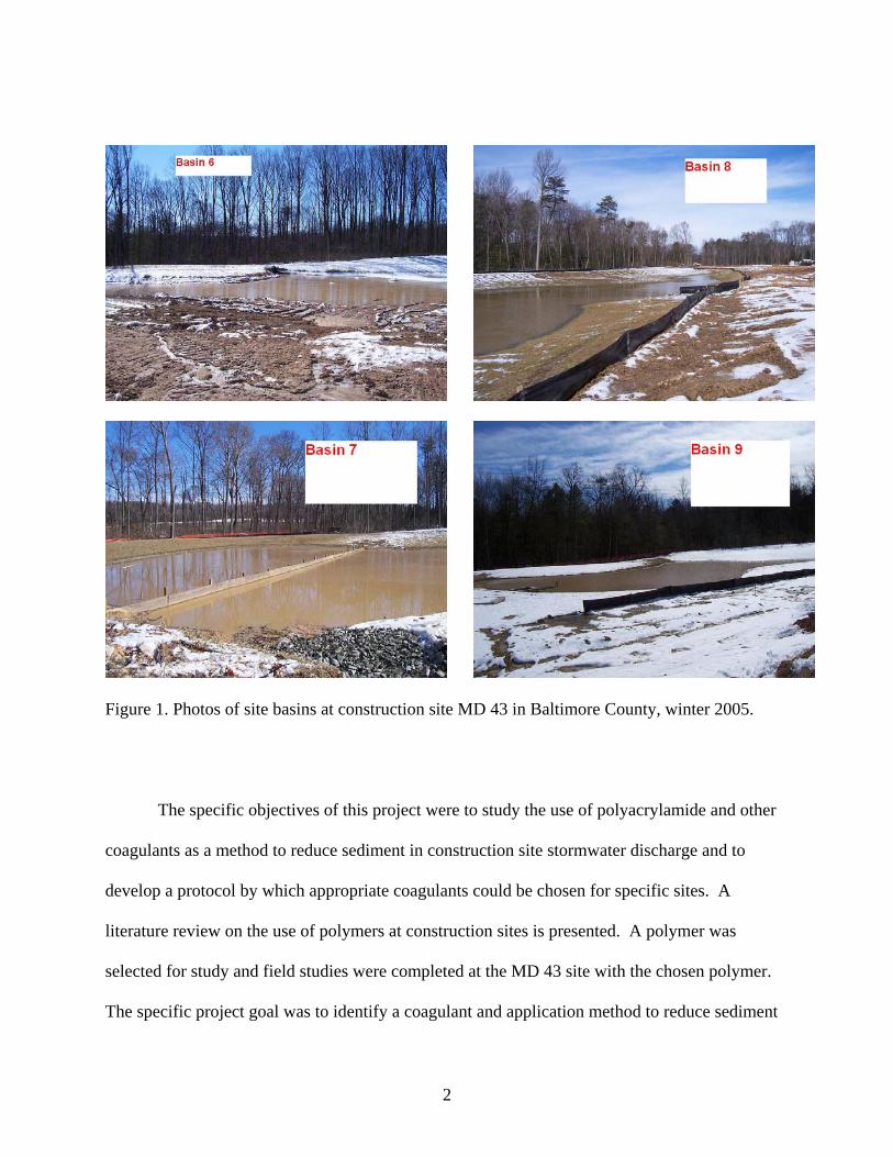
Figure 1. Photos of site basins at construction site MD 43 in Baltimore County, winter 2005.
The specific objectives of this project were to study the use of polyacrylamide and other
coagulants as a method to reduce sediment in construction site stormwater discharge and to
develop a protocol by which appropriate coagulants could be chosen for specific sites. A
literature review on the use of polymers at construction sites is presented. A polymer was
selected for study and field studies were completed at the MD 43 site with the chosen polymer.
The specific project goal was to identify a coagulant and application method to reduce sediment
2

from construction stormwater pond discharges. Parameters needing study include type of
coagulant, dose, effectiveness, application method, and environmental fate of the coagulant
chemical.
Literature Review
Sedimentation
Sedimentation is a solid-liquid separation process. From a water treatment perspective
sedimentation is used mainly to lower the solids concentration before filtration (Gregory et al.
1999). For sedimentation basins, the solids concentration is lowered before discharge to local
streams and wetlands. The term settling is used to describe particles falling through a liquid
under the force of gravity (Gregory et al. 1999). When particles are suspended they may form
flocs with other suspended particles, which increases their settling rate.
Coagulation
Coagulation is a process that is an essential component of water and wastewater
treatment. It is defined as the increase in tendency of small particles in aqueous solution to
attach to one another and to attach to surfaces (Letterman et al. 1999). The physical process of
producing interparticle contacts is termed flocculation. A floc is an agglomeration of small
particles. Coagulants are used to destablize particle suspensions and enhance the rate of floc
formation. Today in water treatment, the list of coagulants is extensive and includes alum, ferric
iron salts, and synthetic and natural organic compounds. Enhanced floc size will often increase
sedimentation rate.
3

Polyacrylamide
Polyacrylamides are a class of water-soluble synthetic compounds formed by the
polymerization of acrylamide monomer. The molecular weight of these compounds can vary
widely, from less than 105 g/mol to greater than 5x10⁶ g/mol (Barvenik 1994). The polymer can
be cationic, anionic, or nonionic. Cationic and anionic polyacrylamides are produced by the
copolymerization of acrylamide and a suitable cationic or anionic comonomer (Figure 2).
Nonionic polyacrylamides are homopolymers of identical acrylamide units with a slight anionic
charge due to hydrolysis (Barvenik 1994). All polyacrylamides contain residual acrylamide, but
it is regulated to <0.05 % by weight.
Figure 2. Anionic Polyacrylamide www.naicc.org/Meeting/ 2001/UseofPAM.html
Polyacrylamide Uses in Water Treatment and Erosion Control
Polyacrylamides were first used in the 1950s when the nonionic form was used to
separate silica fines from dissolved uranium ores in acidic systems (Barvenik 1994). Now
polyacrylamides are used as flocculant aids to primary coagulants in a variety of systems.
Anionic forms are used in mineral and coal processing, petroleum production, papermaking,
water treatment, and food processing. The cationic forms are used for flocculation of sewage
sludge and various industrial wastes (Barvenik 1994). The use of polyacrylamides for erosion
4

control is relatively recent, but now 4x10⁵ ha/year of agricultural land are treated with
polyacrylamide in the United States (Vacher et al. 2003). Polyacrylamide stabilizes soil
aggregates, has been shown to prevent surface seal formation, and increase infiltration of
irrigation water and rainfall (Vacher et al. 2003). With furrow irrigation systems,
polyacrylamide is applied to the irrigation water and applied through a sprinkler system
(McLaughlin 2002). At construction sites, polyacrylamide has been added directly to the soil to
prevent erosion. It can be applied in dry granular form placed on the soil, or in solution and
sprayed onto the soil. In Washington, Minton and Benedict (1999) treated runoff water directly
with polymers. This process resembled a water treatment plant with the basin being a holding
cell, preceding a separate treatment cell.
Polyacrylamide Application Methods
Polyacrylamides have been applied to construction soils in several ways. A Wisconsin
study tested three methods of application. The wet method involved mixing 2.25 g of polymer
with 5 L of water and application with a sprayer or sprinkler. The dry method directly applied
2.25 g of granular polymer to the soil. The mulch method used a polymer solution in
conjunction with a mulch/seeding mix. The mixture was applied using the same methodology as
a typical mulching process. In this study, the mulch method was most effective at reducing
sediment yield (Roa-Espinosa et al.1999). A similar study in Washington found that mixing 120
mg/L polymer with hydromulch produced the highest turbidity reduction, but it was more cost-
effective to use polyacrylamide directly in 40-80 mg/L solution applied at a rate of 6700 L/ha
(720 gal/acre) (Tobiason et al. 2000). Dry polymer was also effective but required 10 times the
material by weight.
5

Another Washington study treated the runoff as opposed to the soil. After the runoff was
collected in a storage pond, it was pumped into a treatment cell where polymer was added to a
concentration of 10-60 mg/L in the basin. (Minton and Benedict 1999). In New Zealand, a
rainfall-driven dosing device was used in stormwater basins (Auckland Regional Council 2003).
Rain would be collected in a tray and flow to a displacement tank. The displacement tank
floated in a polymer solution and the solution was released into the basin when rain entered the
tank. Another trial in New Zealand placed polymer bricks in the inlet channels of the sediment
basins. The runoff was diverted into the channels where it would come into contact with the
polymer before entering the pond (Auckland Regional Council 2003).
Polyacrylamide Effectiveness
The effectiveness of polyacrylamide on erosion control is related to the clay content of
the soil and the molecular weight and charge density of the polymer (Vacher et al. 2003). A
North Carolina study found polyacrylamide to significantly increase total infiltration under
rainfall, reduce surface hardness, and reduce sediment entrainment and erosion by both rainfall
and overland flows when applied directly to the soil surface (McLaughlin 2002). In that study,
the Cytec Superfloc A-100 ranked among the top three flocculants for 10 of 13 sediment sources
and was the top flocculant for 5 sources. The Superfloc polymers were applied at concentrations
of 0.5, 1.0, and 2.0 mg/L to soil solutions in the laboratory and reduced turbidity by up to 99% at
optimal concentrations for the soil type. In the Wisconsin application method study, the mulch
method reduced sediment yield by 93% and the worst polymer application reduced yield by 77%
(Roa-Espinosa et al. 1999).
In Washington, 40 mg/L of polymer solution reduced turbidity of runoff by 72% while
80 mg/L reduced turbidity by 82% (Tobiason et al. 2000). The treatment cell process was able to
6

reduce turbidity from >1000 NTU to <50 NTU for 20-60 mg/L polymer (Minton and Benedict
1999). In the New Zealand study, the use of the polymer bricks was effective at reducing TSS
by up to 50% for inflows of 2 L/s per brick used (Auckland Regional Council 2003). However,
the bricks often broke and washed into the ponds where they were not effective. Also, if
underdosed, the polymer did not significantly reduce TSS. New bricks would need to be placed
before each storm event after estimating the expected inflow rate.
Polyacrylamide Environmental Fate and Toxicity
The toxicity of polyacrylamide in the environment is dependent upon the charge of the
molecule, while the environmental fate is similar for all the polymers. Polyacrylamide can be
degraded in soil systems by cultivation, sunlight, mechanical breakage in the soil, chemical and
biological hydrolysis, salt, and temperature effects (Barvenik 1994, Seybold 1994). This rate has
been estimated at ten percent per year (Barvenik 1994). The polymers have shown to be
resistant to microbial degradation (Seybold 1994). Polyacrylamide is nontoxic to humans when
ingested, but can be a mild skin irritant. The anionic form has been found to have no adverse
effects on fathead minnows, rainbow trout, yellow perch, and bluegill at concentrations of 1000
mg/L for 5 days and 100 mg/L for 90 days (Seybold 1994). Anionic polyacrylamide was only
found to be toxic to fish at concentrations where the water was made viscous and extreme doses
of 1-5 % dry weight of the soil can affect plant growth. Cationic polyacrylamide can bind to the
gills of fish at concentrations of 0.3-10 mg/L. The major concern with polyacrylamide is the
potential for the acrylamide monomer to accumulate in the environment. Acrylamide is a
neurotoxin to humans and highly toxic in the environment. Seybold (1994) says that while
acrylamide is released into the environment via polyacrylamide products, it is biodegradable and
7

does not accumulate in soils. McLaughlin (2002) states that polyacrylamide will not regenerate
the acrylamide monomer in the environment.
Alum
Alum is an aluminum sulfate that is often used for coagulation in water and wastewater
treatment. It has the chemical formula Al2(SO4)3 • nH2O. The number of water molecules of
hydration (n) varies, but is usually 14 or 18 for coagulation purposes. On average, alum is 4.3 wt
% aluminum and has a calculated acidity of 0.111 meq/mg Al (Letterman et al. 1999). In water
and wastewater treatment, alum has been added as a coagulant to turbid water for over 100 years
(Harper et al 2002). Typically it is added as a solid hydrate directly to the water to be treated.
More recently, alum has been added to lakes and stormwater retention ponds as a coagulant, but
also for phosphorus removal.
Chemistry of Alum Coagulation
The primary use of alum is for coagulation. When alum is added, the desired result is an
increased sedimentation rate. To increase the sedimentation rate, the particles must increase in
size through the formation of flocs. Alum precipitates aluminum hydroxide onto the particle
which destabilizes the particle suspension to form flocs through charge neutralization. The vast
majority of natural particles have an inherent charge. This charge is due to isomorphic
substitution, the ionization of amphoteric surface groups for inorganic molecules, or the
ionization of organic functional groups in organic molecules. This charge is pH dependent and is
negative for most particles at natural pH levels. The pH at which a particle charge changes from
positive to negative is known as the pHzpc. For clay, sand, and bacteria, the pHzpc is around 2.
For proteins and other organic matter, it is around 4.5. Alum is an effective coagulant because
aluminum hydroxide has a pHzpc of 8.5 so it maintains a positive charge at most natural pH
8

levels. Once the particle is neutralized, van de Waals attractive forces begin to dominate in the
system. The flocs begin to form and the particles settle out.
When alum is added to water, a series of hydrolysis reactions take place before aluminum
hydroxide is formed (VanLoon and Duffy 2000).
Al(H2O)63+ (aq) + H2O Al(H2O)5(OH)2+ (aq) + H3O+ (1)
Al(H2O)5(OH)2+ (aq) + H2O Al(H2O)4(OH)2+ (aq) + H3O+ (2)
Al(H2O)4(OH)2+ (aq) + H2O Al(H2O)3(OH)3 (s) + H3O+ (3)
Al(H2O)3(OH)3 (s) + H2O Al(H2O)2(OH)4- (s) + H3O+ (4)
The hydrolysis consists of the successive deprotonation of the hydrate molecules around
the aluminum. The extent of the overall reaction is dependent upon the availability of proton
acceptors, usually Bronstead bases. In water, a high alkalinity will often provide the necessary
Bronstead bases for the reaction to proceed fully. In domestic wastewater, high alkalinity is
generally not an issue. However, with stormwater the pH and alkalinity can be variable
depending of the geography, soil, and acidity of the rainfall. Very little if any polymerization
occurs during the hydrolysis (Van Benschoten and Edzwald 1990a). If bicarbonate is used as the
Bronstead base, the overall reaction that takes place is (VanLoon and Duffy 2000):
Al(H2O)63+ (aq) + 3HCO3
- Al(OH)3 (s) + 3CO2 (g) + 6H2O (5)
An example of a potential charge neutralization of silica (SiO2) by alum through polymer
adsorption can be seen as (Letterman et al. 1999):
Al3+ + ≡SiO- + 2H2O ≡SiO-Al(OH)2+ + 2H+ (6)
9

Silica gains its negative charge from negative surface sites such as SiO-. The positively charged
Al(OH)2+ ion bonds with the surface site and neutralizes the charge. A 2005 study showed alum
to have a rapid affect on lowering pH, alkalinity, and dissolved silca concentrations in lakes
(Berkowitz et al. 2005).
The removal of fulvic acid (FA, organic material in water) is slightly more complicated.
When alum is added to remove fulvic acid, it is postulated that a complex of Al(OH)2.7FA0.64 is
formed (Van Benschoten and Edzwald 1990b). This was based on experiments at pH levels of 5
and 7. This same study also determined that removal of fulvic acid is greater at pH 7 than at pH
5.
Another method through which aluminum hydroxide can aid the settling of suspended
particles is through a “sweeping floc.” If a significantly large dose of alum is provided, the
aluminum hydroxide forms large flocs with itself. The flocs then begin to settle and entrap other
suspended particles during the descent. This method is very effective and will reduce the
turbidity of the solution.
When adding alum to a solution, it is advantageous to have the pH between 5.5 and 7.5.
This ensures that aluminum hydroxide will be precipitated rapidly and that the dissolved Al3+
concentration will remain low. A study by Van Benschoten and Edzwald (1990a) demonstrated
that Al solubility was adequately described with only three monomeric species: Al3+, Al(OH)2+,
and Al(OH)4- The U.S. EPA maintains a secondary drinking water standard for aluminum at 1.9-
7.4 x 10⁻⁶ M (0.05-0.20 mg/L). These levels can be reached at pH 5 or 8. It has been reported
that at high pH levels, 3.7 x 10⁻⁶ M (0.01 mg/L) Al may be toxic to trout (Berkowitz et al. 2005).
With alum addition to stormwater, pH will likely decline slightly. This has the potential to
10

decrease the pH and increase the dissolved aluminum concentration to unsafe levels for living
organisms.
Besides pH, the temperature of the system should also be considered when adding alum
as a coagulant. Temperature has been shown to have an effect on turbidity, electrophoretic
mobility, and Al solubility (Van Benschoten and Edzwald 1990a). This difference can be
attributed to the hydroxyl ions involved in the hydrolysis. At constant pH, the hydroxyl ion
concentration changes with temperature as the ion product of water changes with temperature.
However, adverse effects of colder temperatures can be compensated with an increase in pH.
Alum Turbidity Reduction
While the primary focus of most stormwater studies has been phosphorus removal, a
reduction of turbidity can be a benefit of alum use as well. Harper et al (2002) were able to
reduce turbidity and total suspended solids to greater than 97 % removal using alum. This
process could prove to be very useful in the treatment of stormwater retention ponds that have
been overloaded. The pH of stormwater can be variable, but is often within the optimum range
of 5.5-7.5 for alum-induced coagulation.
Methodology
Polymers Used
The literature review noted that several construction sites had shown success at reducing
construction site erosion with the use of polyacrylamide. The nonionic and anionic forms are
nontoxic to aquatic organisms unlike the cationic form. Based on previous studies, anionic
polyacrylamide was chosen to be the focus in this study. Polyacrylamides from Cytec Industries
were used in the field trial and the lab trials. Polymers obtained included Superfloc N-300, a
11

nonionic polyacrylamide, and Superflocs A-100, A-110, A-120, A-130, A-130V, and A-150, all
anionic (Table 1). The anionic charge increases with the higher-numbered polymers. Cationic
polymers C-446, C-448, C-496, and C-498 were also tested for comparison purposes. For the
field trial, A-100 was used because it was compatible with more soil types than any other
polymer used during the North Carolina study (McLaughlin 2002).
Table 1. Characteristics of Polymers employed in the study
Polymer Charge Molecular Weight
N-300 < - 1 % High
A-100 - 7 % High
A-110 - 16 % High
A-120 - 25 % High
A-130 - 33 % High
A-130V - 34 % Ultra High
A-150 - 50 % High
C-446 + 35 % Medium
C-448 + 55 % Medium
C-496 + 35 % High
C-498 + 55% High
Alum
Alum was chosen as an alternative coagulant after the initial polymer laboratory studies.
It was selected based on the known use and performance in water and wastewater treatment and
12

a preliminary lab trial demonstrated effectiveness. The alum used in the laboratory studies was
Al(OH)3 •18H2O, manufactured by Fisher Scientific.
Basin Characteristics
Each basin studied at the Rt. 43 site possessed characteristics that identified it as unique
to the others. Basin 6 had 2 inflows and a rectangular weir outflow. It was the smallest basin in
the study. Basin 7 also had 2 inflows and a rectangular weir outflow, but also had a large baffle
in the middle of the basin to extend the retention time of the runoff and increase mixing. Basin 8
only had one inflow and was long and narrow. The mixing characteristics were expected to be
similar to a plug-flow reactor. Basin 9 was unique in that it had a square overflow weir as
opposed to a rectangular weir. Details are presented in Table 2.
Table 2. Sediment Basin Characteristics at Rt. 43 Construction Site
Basin Surface Area (ft2) Inflows Outflow
Basin 6 25580 2 Rectangular weir
Basin 7 30530 2 Rectangular weir
Basin 8 53860 1 Rectangular weir
Basin 9 42790 1 Square overflow weir
Field Study without Polymer
A control study was performed at the field site without polymer to assess the settling in
the basins. On May 5, 2005, samples were collected every hour for six hours during a rainfall
event from three points in each basin. The sampling locations were, for each basin: the major
input, next to the clothed outlet pipe, and the outflow. The samples were collected in 500 mL
plastic bottles and transported to the Environmental Engineering laboratory at the University of
13

Maryland, College Park in a cooler. Each bottle was rinsed with basin water before the sample
was taken. At the lab, a Total Suspended Solids (TSS) measurement was taken.
Field Study with Polymer
A study was performed at the field site with polymer to assess the feasibility of a large-
scale dosing of a basin. On June 3, Superfloc A-100 was added to basin 7, with basin 6 used as a
control. Six doses of 144 g of polymer were used for a total of 0.864 kg and a total estimated
dose of 1 mg/L in the basin. The dose was calculated using the design volume for basin 7. Each
dose of polymer was placed in a bucket with the bucket then filled with outflow water. The
polymer was mixed in the water and thrown into the basin. The doses were spread throughout
the basin to encourage mixing. A day with light rain was chosen for testing so there would be a
steady inflow into the basins. Samples were collected and transported in the same manner as in
the field study without polymer. Samples were taken just before the polymer was input into
basin 7, and every hour for the following five hours. In basin 6, no sample was taken from the
outflow because there was very little water exiting the basin.
Laboratory Tests
At the site, 500 mL plastic bottles were filled from the edge of basin 9 on June 28, July
20, October 10, November 23, and December 14, basin 8 on July 5, and October 22, and basin 6
on November 23. At the lab, the samples were mixed into labeled plastic bottles, each sample
500 mL. A TSS measurement was taken for each of the samples as well as a Total Dissolved
Solids (TDS) measurement. The appropriate dose of polymer was then added to each sample
from a stock solution of 500 mg/L. A mini-vortex was used to mix the samples after addition for
three minutes. After two hours of settling, TSS and TDS measurements were again taken by
14

siphoning liquid from the top of the sample. After 24 hours of settling, the collection for TSS
and TDS was repeated. An additional sample was taken at this time for a turbidity measurement.
Coagulant Comparison and pH Study Laboratory Tests
The purpose of this protocol development is to select a coagulant and application dose for
use in sedimentation basins. Sediment characteristics vary with each individual site, so this
protocol should be followed to determine the optimum coagulant for use at a particular site. This
protocol was also used for the pH study to maintain similar initial TSS and turbidity conditions
over all pH ranges.
For the tests, enough soil was collected from the drainage area of basin 7 to nearly fill a 5
gallon bucket. This insured there was enough soil for multiple trials. The soil was allowed to air
dry overnight and sieved to 150 μm sieze size. With larger sieve sizes the soil settles too easily
due to high sand content and large flocs of clay and silt. Smaller sizes leave minimal soil to
work with. The action of the coagulants must be focused on clays and silts.
Stormwater was collected in 500 mL plastic bottles from basin 7 on April 14 and May 5
for each coagulant tested plus a no-coagulant control. For the pH study, small amounts of 0.1
HCl or 0.1 NaOH were added to the samples to adjust the pH. The ambient pH of water
collected on 5/4/06 was 7.45.
Three grams of sieved soil were added to 500 mL of relatively clean stormwater collected
from the basin. It was rapidly mixed by shaking the bottle for 5 seconds and allowed 1 minute
for initial settling of sand and other fast-settling particles. Measurements were taken of TSS,
TDS, and turbidity for initial conditions following Standard Methods (2540D, 2540C, 2130B
respectively) procedures (APHA et al. 1999).
15

Coagulants were made into stock solutions with concentrations large enough so that less
than 5 mL of coagulant needed to be added to the sample. A-100 and A-110 had concentrations
of 500 mg/L, C-448 had a concentration of 660 mg/L and alum had a concentration of 11,000
mg/L. The proper coagulant dose was input into water and rapidly mixed using the same
shaking method from the initial testing. Thirty minutes of settling were allowed before repeating
TSS, TDS, and turbidity measurements.
Methodology
A Total Suspended Solids (TSS) measurement was made for all the samples taken. The
procedure was performed following Standard Methods 2540D (APHA et al. 1999). This
measurement collected all suspended solids larger than 1 μm on a filter that was dried at 103-
105oC and weighed.
A Total Dissolved Solids (TDS) measurement was made in the laboratory trials with
polyacrylamide. This procedure was performed following Standard Methods 2540C (APHA
1999). This measurement evaporated the effluent passing through a 1 μm filter, collecting all
dissolved particles as well as suspended particles smaller than 1 μm. The addition of TSS and
TDS produces a Total Solids measurement that is used to standardize the data.
A turbidity measurement was taken for the laboratory trials with polyacrylamide after 24
hours of settling. The measurement was taken using a Hach turbidimeter and followed Standard
Methods 2130B (APHA et al. 1999). The turbidimeter was calibrated using the 17 NTU
standard for measurements between 10 and 100 NTUs and the 2 NTU standard for measurements
between 1 and 10 NTUs.
16

Results
Field Tests
The first field study on May 5 compared the settling effects of the basins. The TSS
measurements taken over six hours at each point in the basin were averaged and are plotted in
Appendix Figure 1. Basin 6 had very low TSS (mean = 55 mg/L) and showed no evidence of
settling. Basins 7 and 8 demonstrated settling in the basins with little effect between the clothed
pipe and the outflow. Basin 9, however, had very high TSS (mean = 964 mg/L). A decrease in
TSS was seen from settling and from the clothed pipe at the outflow. The TSS in the outflow
varied significantly over the 6-hour period of study, but averaged lower than the samples taken
from the clothed pipe.
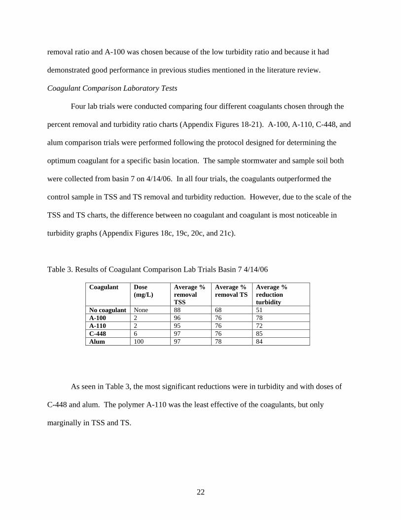
The next field study on June 3 was done with polyacrylamide addition. Samples were
taken from basins 6 and 7, then polymer was input into basin 7. The results can be seen in
Appendix Figures 2a and 2b. A significant change was noted in the inlet flow of basin 7 before
the third hour. However, no effect was seen in the outflow. Visually, the polymer had no affect
on the basin water quality. Basin 6 had very clean input from the recently paved road with very
low TSS (<25 mg/L). Very little settling occurred in the basin with TSS at the clothed pipe
being slightly higher than the input. Overall, the polymer did not demonstrate a significant effect
on the settling in basin 7.
Laboratory Tests
The first samples taken in laboratory studies were tested only for TSS. Through these
experiments, it became apparent that TSS was not the proper measurement for these particular
stormwater ponds. Many of the sediment particles were passing through the 1 μm filter into the
effluent. Upon adding the polymer, these particles would flocculate, but not settle. The
17

subsequent TSS measurement indicated that TSS had increased with settling time because the
agglomerated small particles now did not pass through the TSS filter. With the addition of a
TDS measurement, the samples could be normalized by plotting Total Solids. Since dissolved
solids are changed insignificantly by the polymer addition, the Total Solids chart best represents
the suspended solids present in the samples.
The nonionic polyacrylamide N-300 was tested with stormwater from basin 9 collected
on June 28. After 24 hours of settling, there were negligible differences between the use of the
polymer and no polymer in TS and TSS measurements (Appendix Figures 3a and 3b). After 24
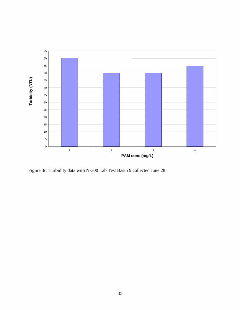
hours, the turbidity also showed no significant difference (Appendix Figure 3c).
The anionic polyacrylamide A-110 was tested with stormwater from basin 9 collected on
June 28th. After 24 hours of settling, a slight decrease in TS (although not in TSS) was noted
with polymer use (Appendix Figures 4a and 4b). However, this difference was not noticed in the
turbidity measurement (Appendix Figure 4c).
Anionic polyacrylamide A-120 and A-100 were tested with stormwater from basin 8
collected on July 5. The runoff sediment on this date was very sandy and significant settling was
observed in all samples. In both cases no difference was noticed in the settling with or without
polymer after 2 hours or after 24 hours (Appendix Figures 5a and 5b, Appendix Figures 6a and
6b). For A-120, the turbidity difference was negligible as well (Appendix Figure 5c). For
A-100, the measured turbidity for the sample without polymer was higher than the samples with
polymer, but the visual difference was negligible at such low turbidity values (Appendix Figure
8c).
Anionic polyacrylamide A-130 and A-150 were tested with stormwater from basin 9
collected on July 20. A slight increase in settling efficiency was noticed in the TS measurement
18

for A-130 concentrations of 0.5 and 1.0 mg/L (Appendix Figures 7a and 7b). However, the
turbidity data did not reflect this difference (Appendix Figure 7c). For A-150, a slight decrease
in TS concentration corresponded with an increase of polymer concentration (Appendix Figures
8a and 8b). Again, this difference was not manifested in the turbidity measurements (Appendix
Figure 8c).
The polymer Superfloc A-150 was retested at high concentrations because of the
promising results at a dose of 2 mg/L (Appendix Figure 9a). Stormwater collected from basin 9
on 10/10/05 was tested with doses of 0, 2, 4, 6, 8, and 10 mg/L. A dose of 2 mg/L demonstrated
a decrease in TS and turbidity (Appendix Figure 9b and 9c). However, the TS and turbidity
increased with higher doses of polyacrylamide. A dose of 2 mg/L is likely the optimum dose of
A-150 for the sediment.
Two tests were performed with alum using doses of 0, 20, 40, 60, 80, and 100 mg/L.
Stormwater collected on 10/10/05 from basin 9 had high initial TS of about 600 mg/L, while
stormwater collected from basin 8 on 10/22/05 had low initial TS of about 175 mg/L (Appendix
Figures 10b and 11b). Both tests displayed similar results for TS and turbidity (Appendix
Figures 10c and 11c). There was a steady decrease in TS and turbidity corresponding with an
increase in alum dosage indicating effective coagulation/flocculation. A more significant
decrease in TS and turbidity was noted after 40 mg/L with very low turbidities noted at 80 and
100 mg/L, 5 NTU and 4 NTU respectively (Appendix Figure 11c). Thus alum showed promise
as a potential coagulant for field testing.
The polymer Superfloc A-130V was tested because it had an “ultra high” molecular
weight. Stormwater collected from basin 9 on 11/23/05 was high in TS, about 550 mg/L and low
in TSS, about 60 mg/L (Appendix Figures 12a and 12b). A comparison of the lab trials illustrate
19

that A-130V had little effect on TSS, TS, or turbidity (Appendix Figures 12a, 12b, and 12c).
Though the differences are slight, the sample with no coagulant had the greatest removal of TSS,
while the sample with 10 mg/L of A-130V had the greatest removal of TS. Turbidity values
were all small and turbidity reductions were negligible for all doses.
The polymer Superfloc C-446 was tested using stormwater collected from basin 9 on
11/23/05. These samples had lower TS values than those collected the same day and used in the
A-130V trial. At doses of 4 mg/L and higher, C-446 demonstrated significant removal of TSS
and TS and lowered turbidity more than no coagulant (Appendix Figures 13a, 13b, and 13c). A
dose of 8 mg/L appeared to be optimal on all three tests, reducing TSS to <4 mg/L, TS to 169
mg/L and turbidity to 1 NTU.
The polymer Superfloc C-496 was tested using stormwater collected from basin 9 on
11/23/05. These samples were similar in initial measurements to those used in the C-446 trial
collected the same day. At a dose of 6 mg/L, the final TSS value was measured to be negative.
This is likely the result of a low TSS value below the detection limit. There was very little
sediment noted on the filter. This affects the TS calculation for that dose and gives the false
impression that a dose of 6 mg/L removed TS better than it actually did. However, a dose of 6
mg/L still had the best removal of TSS and TS (Appendix Figures 14a and 14b). Turbidity
measurements showed minimal differences between the doses (Appendix Figure 14c).
The polymer Superfloc C-448 was tested using stormwater collected from basin 9 on
12/19/05. A comparison of TSS, TS, and turbidity tests demonstrate that doses of 6 mg/L and
higher perform best with doses of 6 and 8 mg/L performing slightly better than 10 mg/L
(Appendix Figures 15a, 15b, and 15c). After 24 hours settling, doses 6 and 8 mg/L lowered TSS
20

to 3 mg/L vis-a-vis the 19 mg/L of no coagulant. The turbidity had been reduced to 2 and 3
NTU respectively, while, the water with no coagulant added had a turbidity of 35 NTU.
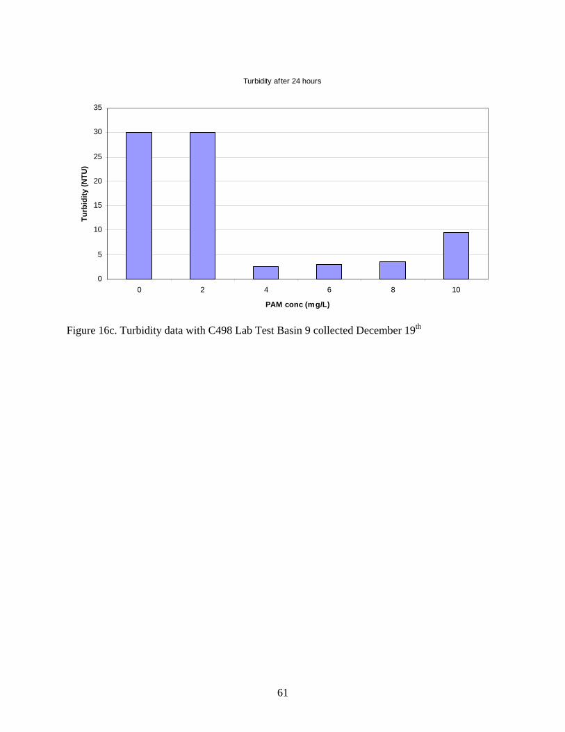
The polymer Superfloc C-498 was tested using stormwater collected from basin 9 on
12/19/05. The TSS trial showed a 4 mg/L dose with the best removal, with other doses having
negligible removal compared to no coagulant (Appendix Figure 16a). The TS trial shows
significant removal for doses of 4, 6, and 8 mg/L (Appendix Figure 16b). The turbidity
measurement shows significant reductions at doses 4 mg/L and above (Appendix Figure 16c).
Percent removal and turbidity ratios
One method of normalizing the initial polymer and alum data is to take ratios comparing
the results using polymer to those of the control. For turbidity, the ratio of coagulant to no
coagulant for final turbidity after 24 hours settling was charted (Appendix Figure 17a). A low
ratio is desirable in this case. The lowest ratios were seen in C-448, C-498 and alum. The best
anionic polymer ratios were A-100 and A-120, but they were significantly higher than the
cations and alum. Percent removal due to TS was calculated for all coagulants and compared to
the percent removal of the control sample of the same trial. These percent removals were than
compared no-coagulant to coagulant addition so a small ratio was desired (Appendix Figure
17b). The lowest ratios were noted by A-110 and alum. C-448 and C-498 cationic polymers
also had low ratios. No other coagulants had ratios less than 0.5.
These ratios determined the coagulants used in the subsequent comparison trial. Since
alum had good ratios in both percent removal and turbidity it was selected immediately. Both
C-448 and C-498 had good ratios, but only one cationic polymer was desired. C-448 was chosen
due to its lower turbidity ratio. Anionic polymer A-110 was chosen based on the percent
21
removal ratio and A-100 was chosen because of the low turbidity ratio and because it had
demonstrated good performance in previous studies mentioned in the literature review.
Coagulant Comparison Laboratory Tests
Four lab trials were conducted comparing four different coagulants chosen through the
percent removal and turbidity ratio charts (Appendix Figures 18-21). A-100, A-110, C-448, and
alum comparison trials were performed following the protocol designed for determining the
optimum coagulant for a specific basin location. The sample stormwater and sample soil both
were collected from basin 7 on 4/14/06. In all four trials, the coagulants outperformed the
control sample in TSS and TS removal and turbidity reduction. However, due to the scale of the
TSS and TS charts, the difference between no coagulant and coagulant is most noticeable in
turbidity graphs (Appendix Figures 18c, 19c, 20c, and 21c).
Table 3. Results of Coagulant Comparison Lab Trials Basin 7 4/14/06
Coagulant Dose (mg/L)
Average % removal TSS
Average % removal TS
Average % reduction turbidity
No coagulant None 88 68 51 A-100 2 96 76 78 A-110 2 95 76 72 C-448 6 97 76 85 Alum 100 97 78 84
As seen in Table 3, the most significant reductions were in turbidity and with doses of
C-448 and alum. The polymer A-110 was the least effective of the coagulants, but only
marginally in TSS and TS.
22

Laboratory pH study
A pH study was conducted following the same protocol as the coagulant comparison to
determine the effect of pH on TSS removal and turbidity reduction. A TS test was not performed
for this study. Coagulants A-100, C-448, and alum were tested, along with a no coagulant
control, at pH values of 5.66, 6.5, 7.45, and 8. The ambient pH was 7.45 and 0.1 M HCl and 0.1
M NaOH were used to adjust the pH of the other samples. Very little effect was noticed on TSS
measurements, however for the three coagulants, a pH of 5.66 had slightly less removal than
other levels (Appendix Figures 22a-d). For the control, pH of 7.45 had less removal. There
were also minimal effects on turbidity measurements, but pH 5.66 consistently had slightly less
removal than other values for all samples (Appendix Figures 22e-h).
Analysis
Width vs. Slope Riprap Channel Design
For a coagulant-assisted stormwater basin to be effective in the field the coagulant must
be well mixed with the water. The mixing increases the particle-coagulant interactions, which
increases floc growth and the subsequent removal of TSS and reduction of turbidity. The basins
themselves lack the inherent mixing capacity for the coagulant to be effective, so an alternative
procedure must be developed. Due to the average size of a basin being thousands of cubic feet, a
large mixing device in the pond is likely to be cost prohibitive. Mixing the coagulant with the
runoff as it enters the basin is a more feasible alternative.
Manning's equation was used for the calculation of channel design:
2/13/2)( SRAn
CQ hm= (7)
23

where Q is the volumetric flow rate of the runoff. This was set at 5 ft3/s for design purposes as a
reasonable expected load for a basin. Cm is a conversion factor of 1.49. Manning's n was
determined to be approximately 0.05 for an open riprap channel (Akan 2006). The area of the
channel, A, is defined as the flow area at normal depth. The hydraulic radius Rh is defined as the
area of the flow divided by the wetted perimeter. The slope S is defined as the elevation change
divided by the length of the channel.
The G mixing value equation (Reynolds 1982) was used to calculate head loss per time
in the channel.
2/1][μγ
thG = (8)
where G is the mixing value with units of inverse seconds and the head loss per time is h/t. The
density of water γ is 62.4 lb/ft3 and the viscosity of water μ is 2.7 x 10⁻⁵ lb/ft s at 25o C.
Appendix Figure 23 was developed by using Manning’s equation to solve for the normal
depth of the channel for a given slope. The normal depth is a function of both the hydraulic
radius and the area. The area and normal depth were used to determine the required width of the
channel for the given parameters. The results were then plotted for corresponding widths and
slopes at different G mixing values. The minimum width allowed by Maryland law for a riprap
inflow channel is 3 feet (MDE 1994).
Using Manning’s equation, it was determined that if coagulant is added to runoff into a
properly designed riprap inflow, adequate mixing can be accomplished. Adequate mixing is
generally defined as having a G mixing value between 700 and 1000 s-1 (Reynolds 1982).
Having a G value that high implies sufficient particle collisions. Appendix Figure 23 illustrates
the design relationship between the slope of the inflow and needed width of the channel for
24

adequate mixing. As the G value increases so does the required slope of the inflow channel for
similar channel widths.
Field Testing
The purpose of this study is to test the field implementation of the laboratory analysis.
The concept is to apply a fixed coagulant dose to the incoming runoff regardless of input flow;
therefore flow will control the coagulant addition. The coagulant is added at the top end of a
riprap channel to promote the mixing of the coagulant before it enters the sedimentation basin.
A schematic of the setup is given in Figure 3. For flow monitoring, a v-notch weir at a 120o
angle should be installed at the top of the rip-rap channel that carries the largest flow to the
basin.
A list of necessary equipment, with examples of potential products, is given below:
• Flow sensor – should be compatible with weir and run on internal battery
(example Teledyne Isco 4210 flow meter, contains both sensor and transmitter).
• Flow transmitter – should be compatible with flow sensor and able to transmit
mA signals.
• Digital Dispenser – should be able to receive mA signals and be compatible
with pump (example Masterflex modular digital drive, Cole-Parmer product
number 07592-20).
• Coagulant Pump – should have a pumping range of approximately 1-20 L/s and
be compatible with digital dispenser (example Masterflex easy-load pump head,
Cole-Parmer product number 77601-10).
25

Figure 3. Field Implementation Schematic for Coagulant-assisted Sediment Basins
Field Implementation
Dispenser
Rain GaugeCoagulant
Sediment Pond
Disturbed Area
• Plastic Tubing – should be compatible with pump and enough length to stretch
from the weir to the coagulant storage area (example C-Flex spooled tubing,
Cole-Parmer product number 06427-82).
• Generator – should be capable of running all equipment for at least 6 hours
(example DuroPower DP1200 portable generator).
• Protective housing – should be capable of protecting both the flow transmitter
and the digital dispenser from the outdoor elements and enable technicians to
work with the equipment.
• Coagulant – should be the coagulant chosen based on laboratory tests.
Rip Rap
Weir & Flow
Meter
26

• Coagulant Storage – should be enough coagulant to be used during a 10-year
storm event.
For installation, the flow sensor will be mounted to the weir. A cable must run from the
sensor to the flow transmitter. The transmitter converts the raw data of the sensor into a current
signal that can be read by the digital dispenser. The digital dispenser must be calibrated to
interpret the flow signal and apply the proper amount of coagulant using the pump. A cable
connects the dispenser to the pump. The flow transmitter and the dispenser must be located
inside the protective housing and connected to the generator. For coagulant storage, two or three
55 gallon drums will provide sufficient coagulant for major storms.
An alternative, but less accurate method, would be to use a rain gauge transmitter (Cole-
Parmer product number 99780-60) connected directly to the digital dispenser. This method
would estimate the input runoff flow rate into the basin based on rainfall, rather than measuring
it directly. This method should be used in the event that a weir can not be installed to the inflow.
The digital dispenser will be calibrated for dosing based on the laboratory tests of the
chosen coagulant. Based on the input flow rate of the channel, enough coagulant will be pumped
as to provide the proper dose in mg/L for all of the runoff entering the basin.
Once the field test equipment is installed, monitoring will be conducted through
sampling. Comparative studies will be done by also sampling a basin without coagulant
addition. Grab samples will be collected from the beginning of the input channel (prior to
coagulant addition), where the input channel enters the basin, and at the outflow during a rainfall
event. Sampling should begin soon after rainfall begins and be taken every hour during the
rainfall, preferably for a minimum of 6 hours. Sample bottles should be 500 mL for easy
27

transport and testing. These samples will be tested for TSS, TDS, and Turbidity using Standard
Methods at the University of Maryland, College Park.
Conclusions and Recommendations for Implementation
Based on the laboratory data collected from the Rt. 43 White Marsh site, coagulants can
be effective for reducing suspended solids and turbidity in stormwater basins. For anionic
polyacrylamide, doses of 2 mg/L or less were the most effective. Cationic polyacrylamides
worked best with doses between 6 and 10 mg/L. Alum performed best at a dose of 100 mg/L.
For this particular site, alum was the most effective in both removing suspended solids and
lowering turbidity. Using alum, an average of 97% of TSS was removed compared to 88%
without coagulant. Turbidity was reduced by over 84% with alum compared to only 50%
without a coagulant. However, literature data suggests that soils can be variable in their
interactions with coagulants and what is effective at one site may not be at another. It is
recommended that SHA follow the protocol developed and included in the Appendix. The
protocol describes the process by which to best choose a coagulant for use in stormwater basins.
Field testing research is recommended before widespread implementation of coagulant-assisted
stormwater basins.
This study provides important information to SHA about the potential for coagulant-
assisted stormwater basins for active road construction sites. Laboratory data demonstrated the
efficacy of several coagulants for this use. The removal of additional suspended solids and
turbidity can greatly reduce the pollutant load entering the water bodies near active construction
sites. Continued research into the implementation of coagulant-assisted stormwater basins will
provide additional data into the feasibility of this option as a pollution prevention method.
28

References
Akan, A. Osman. (2006) Open Channel Hydraulics. Elsevier Ltd. Burlington, MA.
American Public Health Association (APHA), American Water Works Association, Water
Environment Federation. (1999). Standard Methods for Examination of Water and
Wastewaters, 20th Ed., APHA, Washington D.C.
Auckland Regional Council. (2003). "The Use of Flocculants and Coagulants to Aid the
Settlement of Suspended Sediment in Earthworks Runoff – Trials, Methodology, and
Design." Auckland, New Zealand
Barvenik, F.W. (1994). “Polyacrylamide Characteristics Related to Soil Applications.” Soil Sci.
158, 235-243
Berkowitz, J., M. A. Anderson, R. C. Graham. (2005). “Laboratory investigation of
aluminum solubility and solid-phase properties following alum treatment of lake
waters.” Water Research 39, 3918-3928.
Gregory, R., J.F. Zabel, J.K. Edzwald. (1999). “Sedimentation and Flotation.” Water Quality and
Treatment, 5th Ed., McGraw-Hill, New York
Harper, H.H., J.L. Herr, and E. Livingston. 1998. Alum treatment of stormwater: The
first ten years. New Applications in Modeling Urban Water Systems. J. Williams
(ed.). Guelph, Ontario: CHI.
Letterman, R.D., A. Amirtharajah, C.R. O’Melia. (1999). “Coagulation and Flocculation.” Water
Quality and Treatment, 5th Ed., McGraw-Hill, New York
Maryland Department of the Environment. (1994) “Maryland Standards and Specifications for
Soil Erosion and Sediment Control.”
29

Minton, G.R., A.H. Benedict. (1999). “Use of Polymers to Treat Construction Site Stormwater.”
International Erosion Control Association Proceedings of Conference 30, Nashville, TN.
177-188
McLaughlin, R.A. (2002) “Measures to Control Erosion and Turbidity in Construction Site
Runoff.” NC Dept. of Trans. and Ctr. For Trans. and Environ. Joint Project 2001-05
Final Report. 131 pages
Reynolds, Tom D. (1982) Unit Operations and Processes in Environmental Engineering.
Wadsworth Inc. Belmont, CA.
Roa-Espinosa, A., G.D. Bubenzer, E.S. Miyashita. (1999). “Sediment and Runoff Control on
Construction Sites Using Four Application Methods of Polyacrylamide Mix.” American
Society of Agricultural Engineers. Paper No. 99-2013
Seybold, C.A. (1994). “Polyacrylamide Review: Soil Conditioning and Environmental Fate.”
Comm. Soil Sci. Plant Anal. 25, 2171-2185
Tobiason, S., D. Jenkins, E. Molash, S. Rush. (2000). “Polymer Use and Testing for Erosion and
Sediment Control on Construction Sites: Recent Experience in the Pacific Northwest.”
International Erosion Control Association Proceedings of Conference 31, Palm Springs,
CA. 39-52
Vacher, C.A., R.J. Loch, S.R. Raine. (2003). “Effect of polyacrylamide additions on infiltration
and erosion of disturbed lands.” Australian Journal of Soil Research. 41, 1509-1520
Van Benschoten, J. E., J. K. Edzwald (1990a). “Chemical aspects of coagulation using
aluminum salts – I. Hydrolytic reactions of alum and polyaluminum chloride.”
Water Research. 24, 1519-1526.
30

Van Benschoten, J. E., J. K. Edzwald (1990b). “Chemical aspects of coagulation using
aluminum salts – II. Coagulation of fulvic acid using alum and polyaluminum
chloride.” Water Research. 24, 1527-1535.
VanLoon, G.W., S. J. Duffy. (2000). Environmental Chemistry. 1st Ed., Oxford
University Press, New York.
31

Appendix: Figures
0.0
200.0
400.0
600.0
800.0
1000.0
1200.0
0 0.5 1 1.5 2 2.5 3 3.5Location: 1=Inlet, 2=Pipe, 3=Outlet
TSS
mg/
L
Basin 6Basin 7Basin 8Basin 9
Figure 1. Average TSS measurements from May 5 field test, error bars ± 1 standard deviation
32
0
20
40
60
80
100
120
140
160
180
200
Hour 1 Hour 2 Hour 3 Hour 4 Hour 5 Hour 6
Time
TSS
(mg/
L)
Inlet
Pipe
Outflow
Figure 2a. TSS data from Basin 7 Field Test June 3 with polymer addition
0
5
10
15
20
25
30
35
Hour 1 Hour 2 Hour 3 Hour 4 Hour 5 Hour 6
Time
TSS
(mg/
L)
Inlet
Pipe
Figure 2b. TSS data from Basin 6 Field Test June 3 without polymer
33

0
10
20
30
40
50
60
70
0 0.5 1 2
PAM conc (mg/L)
TSS
(mg/
L)Before PAM2 hours24 hours
Figure 3a. TSS data with N-300 Lab Test Basin 9 collected June 28
0
50
100
150
200
250
300
350
400
0 0.5 1 2
PAM conc (mg/L)
TS (m
g/L)
Before PAM2 hours24 hours
Figure 3b. TS data with N-300 Lab Test Basin 9 collected June 28th
34
0
5
10 15 20 25 30 35 40 45 50 55 60 65
1 2 3 4
PAM conc (mg/L)
Turb
idity
(NTU
)
Figure 3c. Turbidity data with N-300 Lab Test Basin 9 collected June 28
35

0
5
10
15
20
25
30
35
40
0 0.5 1 2
PAM conc (mg/L)
TSS
(mg/
L)
Before PAM
2 hours
24 hours
Figure 4a. TSS data with A-110 Lab Test Basin 9 collected June 28
0
50
100
150
200
250
300
350
400
0 0.5 1 2
PAM conc (mg/L)
TS (m
g/L)
Before PAM
2 hours
24 hours
Figure 4b. TS data with A-110 Lab Test Basin 9 collected June 28
36

0
5
10 15 20 25 30 35 40 45 50 55 60 65
0 0.5 1 2
Pam conc (mg/L)
Turb
idity
(NTU
)
Figure 4c. Turbidity data with A-110 Lab Test Basin 9 collected June 28
37

0
50
100
150
200
250
300
350
0 0.5 1 2
PAM conc (mg/L)
TSS
(mg/
L)Before PAM
2 hours
24 hours
Figure 5a. TSS data with A-120 Lab Test Basin 8 collected July 5
0
100
200
300
400
500
600
700
0 0.5 1 2
PAM conc (mg/L)
TS (m
g/L)
Before PAM
2 hours
24 hours
Figure 5b. TS data with A-120 Lab Test Basin 8 collected July 5
38

0
1
2
3
4
5
6
7
8
9
0 0.5 1 2
Pam conc (mg/L)
Turb
idity
(NTU
)
Figure 5c. Turbidity data with A-120 Lab Test Basin 8 collected July 5
39

0
50
100
150
200
250
300
350
400
450
500
0 0.5 1 2
PAM conc (mg/L)
TSS
(mg/
L)Before PAM
2 hours
24 hours
Figure 6a. TSS data with A-100 Lab Test Basin 8 collected July 5
0
100
200
300
400
500
600
700
800
900
0 0.5 1 2
PAM conc (mg/L)
TS (m
g/L)
Before PAM
2 hours
24 hours
Figure 6b. TS data with A-100 Lab Test Basin 8 collected July 5
40

0
2
4
6
8
10
12
14
16
0 0.5 1 2
Pam conc ( /L)
Turb
idity
(NTU
)
Figure 6c. Turbidity data with A-100 Lab Test Basin 8 collected July 5
41

0
100
200
300
400
500
600
0 0.5 1 2
PAM conc (mg/L)
TSS
(mg/
L)
Before PAM
2 hours
24 hours
Figure 7a. TSS data with A-130 Lab Test Basin 9 collected July 20
0
100
200
300
400
500
600
700
0 0.5 1 2
PAM conc (mg/L)
TS (m
g/L)
Before PAM
2 hours
24 hours
Figure 7b. TS data with A-130 Lab Test Basin 9 collected July 20
42

0
5
10 15 20 25 30 35 40 45 50 55 60 65
0 0.5 1 2
Pam conc (mg/L)
Turb
idity
(NTU
)
Figure 7c. Turbidity data with A-130 Lab Test Basin 9 collected July 20
43

0
50
100
150
200
250
300
350
400
450
500
0 0.5 1 2
PAM conc (mg/L)
TSS
(mg/
L)Before PAMafter 2 hoursafter 24 hours
Figure 8a. TSS data with A-150 Lab Test Basin 9 collected July 20
0
100
200
300
400
500
600
700
800
0 0.5 1 2
PAM conc (mg/L)
TS (m
g/L)
Before PAMafter 2 hoursafter 24 hours
Figure 8b. TS data with A-150 Lab Test Basin 9 collected July 20
44

0
5
10 15 20 25 30 35 40 45 50 55 60 65
0 0.5 1 2Pam conc (mg/L)
Turb
idity
(NTU
)
Figure 8c. Turbidity data with A-150 Lab Test Basin 9 collected July 20
45

0
50
100
150
200
250
300
350
400
450
500
0 2 4 6 8 10
PAM conc (mg/L)
TSS
(mg/
L)Before PAMafter 2 hoursafter 24 hours
Figure 9a. TSS data with A-150 Lab Test Basin 9 collected October 10
0
100
200
300
400
500
600
700
0 2 4 6 8 10
PAM conc (mg/L)
TS (m
g/L)
Before PAMafter 2 hoursafter 24 hours
Figure 9b. TS data with A-150 Lab Test Basin 9 collected October 10
46

0
15
30
45
60
75
90
105
120
135
0 2 4 6 8 10
PAM conc (mg/L)
Turb
idity
(NTU
)
Figure 9c. Turbidity data with A-150 Lab Test Basin 9 collected October 10
47

0
50
100
150
200
250
300
350
400
450
0 20 40 60 80 100
Alum conc (mg/L)
TSS
(mg/
L)Before Alumafter 2 hoursafter 24 hours
Figure 10a. TSS data with alum Lab Test Basin 9 collected October 10
0
100
200
300
400
500
600
700
800
900
0 20 40 60 80 100
Alum conc (mg/L)
TS (m
g/L)
Before Alumafter 2 hoursafter 24 hours
Figure 10b. TS data with alum Lab Test Basin 9 collected October 10
48

0
15
30
45
60
75
90
105
120
135
0 20 40 60 80 100
Alum conc (mg/L)
Turb
idity
(NTU
)
Figure 10c. Turbidity data with alum Lab Test Basin 9 collected October 10
49

-10
0
10
20
30
40
50
60
0 20 40 60 80 100
Alum conc (mg/L)
TSS
(mg/
L)
Before Alumafter 2 hoursafter 24 hours
Figure 11a. TSS data with alum Lab Test Basin 8 collected October 22
0
50
100
150
200
250
300
0 20 40 60 80 100
Alum conc (mg/L)
TS (m
g/L)
Before Alumafter 2 hoursafter 24 hours
Figure 11b. TS data with alum Lab Test Basin 8 collected October 22
50

0
15
30
0 20 40 60 80 100
Alum conc (mg/L)
Turb
idity
(NTU
)
Figure 11c. Turbidity data with alum Lab Test Basin 8 collected October 22
51

0
10
20
30
40
50
60
70
0 2 4 6 8 10
PAM conc (mg/L)
TSS
(mg/
L)Before PAMafter 2 hoursafter 24 hours
Figure 12a. TSS data with A-130V Lab Test Basin 6 collected November 23
0
100
200
300
400
500
600
700
0 2 4 6 8 10
PAM conc (mg/L)
TS (m
g/L)
Before PAMafter 2 hoursafter 24 hours
Figure 12b. TS data with A-130V Lab Test Basin 6 collected November 23
52

0
5
10
0 2 4 6 8 10
PAM conc (mg/L)
Turb
idity
(NTU
)
Figure 12c. Turbidity data with A-130V Lab Test Basin 6 collected November 23
53

0
10
20
30
40
50
60
0 2 4 6 8 10
PAM conc (mg/L)
TSS
(mg/
L)Before PAMafter 2 hoursafter 24 hours
Figure 13a. TSS data with C-446 Lab Test Basin 9 collected November 23
0
50
100
150
200
250
300
0 2 4 6 8 10
PAM conc (mg/L)
TS (m
g/L)
Before PAMafter 2 hoursafter 24 hours
Figure 13b. TS data with C-446 Lab Test Basin 9 collected November 23
54

0
5
10
15
0 2 4 6 8 10
PAM conc (mg/L)
Turb
idity
(NTU
)
Figure 13c. Turbidity data with C-446 Lab Test Basin 9 collected November 23
55

-30
-20
-10
0
10
20
30
40
50
60
70
0 2 4 6 8 10
PAM conc (mg/L)
TSS
(mg/
L)Before PAMafter 2 hoursafter 24 hours
Figure 14a. TSS data with C-496 Lab Test Basin 9 collected November 23
0
50
100
150
200
250
300
0 2 4 6 8 10
PAM conc (mg/L)
TS (m
g/L)
Before PAMafter 2 hoursafter 24 hours
Figure 14b. TS data with C-496 Lab Test Basin 9 collected November 23
56

0
5
10
0 2 4 6 8 10
PAM conc (mg/L)
Turb
idity
(NTU
)
Figure 14c. Turbidity data with C-496 Lab Test Basin 9 collected November 23
57

0
10
20
30
40
50
60
70
80
90
0 2 4 6 8 10
PAM conc (mg/L)
TSS
(mg/
L)Before PAMafter 2 hoursafter 24 hours
Figure 15a. TSS data with C-448 Lab Test Basin 9 collected December 19
0
50
100
150
200
250
0 2 4 6 8 10
PAM conc (mg/L)
TS (m
g/L)
Before PAMafter 2 hoursafter 24 hours
Figure 15b. TS data with C-448 Lab Test Basin 9 collected December 19
58

0
5
10
15
20
25
30
35
40
0 2 4 6 8 10
PAM conc (mg/L)
Turb
idity
(NTU
)
Figure 15c. Turbidity data with C-448 Lab Test Basin 9 collected December 19
59

0
10
20
30
40
50
60
70
0 2 4 6 8 10
PAM conc (mg/L)
TSS
(mg/
L)Before PAMafter 2 hoursafter 24 hours
Figure 16a. TSS data with C-498 Lab Test Basin 9 collected December 19
0
50
100
150
200
250
300
0 2 4 6 8 10
PAM conc (mg/L)
TS (m
g/L)
BeforePAMafter 2 hoursafter 24 hours
Figure 16b. TS data with C-498 Lab Test Basin 9 collected December 19
60
Turbidity after 24 hours
0
5
10
15
20
25
30
35
0 2 4 6 8 10
PAM conc (mg/L)
Turb
idity
(NTU
)
Figure 16c. Turbidity data with C498 Lab Test Basin 9 collected December 19th
61

0
0.2
0.4
0.6
0.8
1
1.2
N-3001 mg/L
A-1002 mg/L
A-1102 mg/L
A-1200.5
mg/L
A-1301 mg/L
A-130V10
mg/L
A-1502 mg/L
C-44610
mg/L
C-4966 mg/L
C-4486 mg/L
C-4988 mg/L
Alum100
mg/L
Coagulant
ratio
Figure 17a. Ratio of turbidity after 24 hours of coagulant vis-a-vis no coagulant
-0.8
-0.6
-0.4
-0.2
0
0.2
0.4
0.6
0.8
1
1.2
1.4
N-3001 mg/L
A-1002 mg/L
A-1102 mg/L
A-1200.5
mg/L
A-1301 mg/L
A-130V10
mg/L
A-1502 mg/L
C-44610
mg/L
C-4966 mg/L
C-4486 mg/L
C-4988 mg/L
Alum100
mg/L
Coagulant
% re
mov
al w
/o c
oag
: % re
mov
al w
/ coa
g
Figure 17b. Ratio of percent removal TS using no coagulant vis-a-vis coagulant usage
62

0
200
400
600
800
1000
1200
1400
1600
none A-100 2mg/L A-110 2 mg/L C-448 6 mg/L Alum 100 mg/L
Coagulant Conc (mg/L)
TSS
(mg/
L)Before coagulantafter 30 minutes
Figure 18a. TSS data for Comparison Lab Trial 1 Basin 7 collected April 14
0
200
400
600
800
1000
1200
1400
1600
1800
2000
none A-100 2mg/L A-110 2 mg/L C-448 6 mg/L Alum 100 mg/L
Coagulant Conc (mg/L)
TS (m
g/L)
Before coagulantafter 30 minutes
Figure 18b. TS data for Comparison Lab Trial 1 Basin 7 collected April 14
63

0
15
30
45
60
75
none A-100 2mg/L A-110 2 mg/L C-448 6 mg/L Alum 100 mg/L
Coagulant Conc (mg/L)
Turb
idity
(NTU
)before coagulantafter 30 minutes
Figure 18c. Turbidity data for Comparison Lab Trial 1 Basin 7 collected April 14
64

0
500
1000
1500
2000
2500
none A-100 2mg/L A-110 2 mg/L C-448 6 mg/L Alum 75 mg/L
Coagulant Conc (mg/L)
TSS
(mg/
L)Before coagulantafter 30 minutes
Figure 19a. TSS data for Comparison Lab Trial 2 Basin 7 collected April 14
0
500
1000
1500
2000
2500
3000
none A-100 2mg/L A-110 2 mg/L C-448 6 mg/L Alum 75 mg/L
Coagulant Conc (mg/L)
TS (m
g/L)
Before coagulantafter 30 minutes
Figure 19b. TS data for Comparison Lab Trial 2 Basin 7 collected April 14
65

0
15
30
45
60
75
90
none A-100 2mg/L A-110 2 mg/L C-448 6 mg/L Alum 75 mg/L
Coagulant Conc (mg/L)
Turb
idity
(NTU
)before coagulantafter 30 minutes
Figure 19c. Turbidity data for Comparison Lab Trial 2 Basin 7 collected April 14
66

0
500
1000
1500
2000
2500
3000
3500
4000
none A-100 2mg/L A-110 2 mg/L C-448 6 mg/L Alum 100 mg/L
Coagulant Conc (mg/L)
TSS
(mg/
L)
Before coagulantafter 30 minutes
Figure 20a. TSS data for Comparison Lab Trial 3 Basin 7 collected April 14
0
500
1000
1500
2000
2500
3000
3500
4000
4500
none A-100 2mg/L A-110 2 mg/L C-448 6 mg/L Alum 100 mg/L
Coagulant Conc (mg/L)
TS (m
g/L)
Before coagulantafter 30 minutes
Figure 20b. TS data for Comparison Lab Trial 3 Basin 7 collected April 14
67

0
15
30
45
60
75
90
105
none A-100 2mg/L A-110 2 mg/L C-448 6 mg/L Alum 100 mg/L
Coagulant Conc (mg/L)
Turb
idity
(NTU
)before coagulantafter 30 minutes
Figure 20c. Turbidity data for Comparison Lab Trial 3 Basin 7 collected April 14
68

0
500
1000
1500
2000
2500
none A-100 2mg/L A-110 2 mg/L C-448 6 mg/L Alum 100 mg/L
Coagulant Conc (mg/L)
TSS
(mg/
L)Before coagulantafter 30 minutes
Figure 21a. TSS data for Comparison Lab Trial 4 Basin 7 collected April 14
0
500
1000
1500
2000
2500
3000
none A-100 2mg/L A-110 2 mg/L C-448 6 mg/L Alum 100 mg/L
Coagulant Conc (mg/L)
TS (m
g/L)
Before coagulantafter 30 minutes
Figure 21b. TS data for Comparison Lab Trial 4 Basin 7 collected April 14
69

0
15
30
45
60
75
90
105
none A-100 2mg/L A-110 2 mg/L C-448 6 mg/L Alum 100 mg/L
Coagulant Conc (mg/L)
Turb
idity
(NTU
)before coagulantafter 30 minutes
Figure 21c. Turbidity data for Comparison Lab Trial 4 Basin 7 collected April 14
70

0
500
1000
1500
2000
2500
3000
5.66 6.5 7.45 8
pH
TSS
(mg/
L)
InitialAfter 30 minutes
Figure 22a. TSS data for no coagulant Lab Trial pH study Basin 7 collected May 4
0
500
1000
1500
2000
2500
3000
3500
5.66 6.5 7.45 8
pH
TSS
(mg/
L)
InitialAfter 30 minutes
Figure 22b. TSS data for A-100 Lab Trial pH study Basin 7 collected May 4
71

0
500
1000
1500
2000
2500
3000
5.66 6.5 7.45 8
pH
TSS
(mg/
L)
InitialAfter 30 minutes
Figure 22c. TSS data for C-448 Lab Trial pH study Basin 7 collected May 4
0
500
1000
1500
2000
2500
3000
3500
5.66 6.5 7.45 8
pH
TSS
(mg/
L)
InitialAfter 30 minutes
Figure 22d. TSS data for Alum Lab Trial pH study Basin 7 collected May 4t
72

0
20
40
60
80
100
120
5.66 6.5 7.45 8
pH
Turb
idity
InitialAfter 30 minutes
Figure 22e. Turbidity data for no coagulant Lab Trial pH study Basin 7 collected May 4
0
20
40
60
80
100
120
5.66 6.5 7.45 8
pH
Turb
idity
InitialAfter 30 minutes
Figure 22f. Turbidity data for A-100 Lab Trial pH study Basin 7 collected May 4
73

0
20
40
60
80
100
120
5.66 6.5 7.45 8
pH
Turb
idity
InitialAfter 30 minutes
Figure 22g. Turbidity data for C-448 Lab Trial pH study Basin 7 collected May 4
0
20
40
60
80
100
120
5.66 6.5 7.45 8
pH
Turb
idity
InitialAfter 30 minutes
Figure 22h. Turbidity data for Alum Lab Trial pH study Basin 7 collected May 4
74

0
2
4
6
8
10
12
14
0 0.02 0.04 0.06 0.08 0.1 0.12 0.14 0.16Inflow Slope
Inflo
w W
idth
(ft)
G=900G=800G=1000G=600Minimum width
Figure 23. Width vs. Slope ratios for different G mixing values of riprap inflows
75
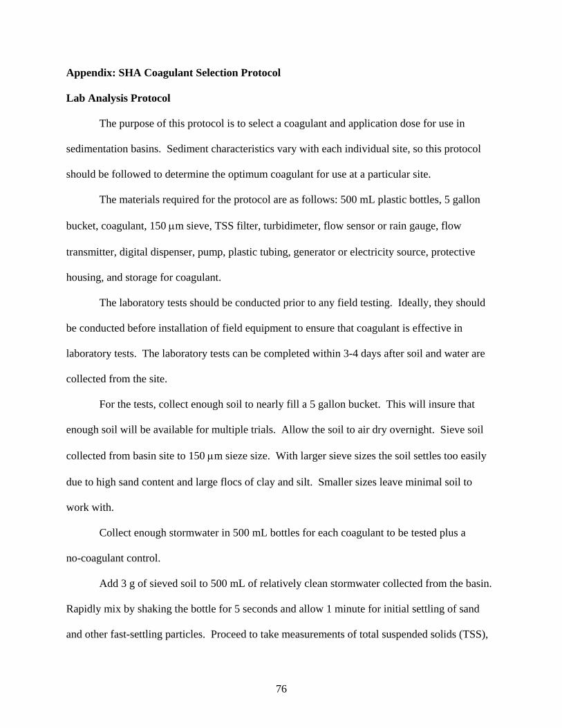
Appendix: SHA Coagulant Selection Protocol
Lab Analysis Protocol
The purpose of this protocol is to select a coagulant and application dose for use in
sedimentation basins. Sediment characteristics vary with each individual site, so this protocol
should be followed to determine the optimum coagulant for use at a particular site.
The materials required for the protocol are as follows: 500 mL plastic bottles, 5 gallon
bucket, coagulant, 150 μm sieve, TSS filter, turbidimeter, flow sensor or rain gauge, flow
transmitter, digital dispenser, pump, plastic tubing, generator or electricity source, protective
housing, and storage for coagulant.
The laboratory tests should be conducted prior to any field testing. Ideally, they should
be conducted before installation of field equipment to ensure that coagulant is effective in
laboratory tests. The laboratory tests can be completed within 3-4 days after soil and water are
collected from the site.
For the tests, collect enough soil to nearly fill a 5 gallon bucket. This will insure that
enough soil will be available for multiple trials. Allow the soil to air dry overnight. Sieve soil
collected from basin site to 150 μm sieze size. With larger sieve sizes the soil settles too easily
due to high sand content and large flocs of clay and silt. Smaller sizes leave minimal soil to
work with.
Collect enough stormwater in 500 mL bottles for each coagulant to be tested plus a
no-coagulant control.
Add 3 g of sieved soil to 500 mL of relatively clean stormwater collected from the basin.
Rapidly mix by shaking the bottle for 5 seconds and allow 1 minute for initial settling of sand
and other fast-settling particles. Proceed to take measurements of total suspended solids (TSS),
76

total dissolved solids (TDS), and turbidity for initial conditions following Standard Methods
(2540D, 2540C, 2130B respectively) procedures (APHA et al. 1999).
Coagulants should be made into stock solutions using deionized water with
concentrations large enough so that less than 5 mL of coagulant needs to be added to the sample.
Input proper coagulant dose into water and rapidly mix using same shaking method again.
Allow 30 minutes of settling before repeating TSS, TDS, and turbidity measurements.
Repeat for each coagulant used and a control with no coagulant. Select the best
coagulant for field testing based on significant decreases in TSS and turbidity.
77