
Robert K. Paasch
91
Transcript of Robert K. Paasch

AN ABSTRACT OF THE THESIS OF
Stephen A. Meicke for the degree of Master of Science in Mechanical Engineering
presented on August 17, 2011.
Title: Hydroelastic Modeling of a Wave Energy Converter Using the Arbitrary
Lagrangian-Eulerian Finite Element Method in LS-DYNA
Abstract approved:
Robert K. Paasch
This thesis investigates the applicability of the finite element method to model wave
energy converter (WEC) hydroelasticity using LS-DYNA. The proposed methodology
uses the Arbitrary Lagrangian-Eulerian formulation to model Fluid-Structure Interaction
(FSI) between the WEC and the fluid elements. This formulation allows for time-domain
modeling of higher order effects such as fluid vorticity and viscosity, and nonlinear /
breaking waves. This document presents initial investigations into: (i) the suitability of
the current FSI simulation capability in LS-DYNA for modeling WECs, (ii) and fluid-
structure coupling methodology, (iii) the development of an improved computational
wave basin, and (iv) realistic mooring and power take-off modeling. This project is the
first stage of an ongoing effort to advance the state of the art in numerical modeling of
WECs and other offshore structures using the finite element methodology. For modeling
efforts continuing in the future, a framework for the eventual validation of numerical
results using experimental data from testing of Columbia Power Technologies 1:33 and
1:7 scale SeaRay WEC is also presented.

©Copyright by Stephen A. Meicke
August 17, 2011
All Rights Reserved

Hydroelastic Modeling of a Wave Energy Converter Using the Arbitrary Lagrangian-
Eulerian Finite Element Method in LS-DYNA
by
Stephen A. Meicke
A THESIS
submitted to
Oregon State University
in partial fulfillment of
the requirements for the
degree of
Master of Science
Presented August 17, 2011
Commencement June 2012

Master of Science thesis of Stephen A. Meicke presented on August 17, 2011.
APPROVED:
Major Professor, representing Mechanical Engineering
Head of the School of Mechanical, Industrial and Manufacturing Engineering
Dean of the Graduate School
I understand that my thesis will become part of the permanent collection of Oregon State
University libraries. My signature below authorizes release of my thesis to any reader
upon request.
Stephen A. Meicke, Author

ACKNOWLEDGEMENTS
We do not inherit the earth from our ancestors,
we borrow it from our children.
~ Native American Proverb
First, I would like to thank my mother, father and sister for always being there for me,
encouraging me in times of need, and for their unconditional love. Mom, thank you for
teaching me about the earth, and the importance of respecting and preserving the land and
every living being for future generations to come. Dad, thanks for teaching me to follow
my heart, and to always do what is right, no matter how hard it may be. Only armed with
the knowledge of our impact on the world, and the resolve to do what we know is right in
our hearts can we hope to preserve this beautiful planet for future generations to come.
To Jennifer – thank you for teaching me the meaning of love, making me smile, and
helping me to appreciate life more fully than ever before. I am looking forward to
spending the rest of my life by your side.
To my office mates and good friends Pukha, Justin, Kelley, Blake – thank you for your
help during countless days of classes and homework, paper writing and editing, and
research projects which seemed to have no end. I couldn‟t have finished without your
help. Yi, Ravi, and Junhui – thank you for taking me in as a fellow LS-DYNA minion,
putting up with my questions, and helping me to work through the innumerable obstacles
of nonlinear finite element analysis.
Funding for this work is greatly appreciated, and was provided by Columbia Power
Technologies, The Northwest National Marine Renewable Energy Center, United States
Department of Energy under Award Number DE-FG36-08GO18179, and the United
States Navy.
TABLE OF CONTENTS
1. Introduction ..................................................................................................................... 1
2. Project Background ......................................................................................................... 5
2.1 – Research and Development of the SeaRay Concept ............................................ 5
2.2 – Strain and Force Transducers ............................................................................... 8
3. Modeling in LS-DYNA ................................................................................................ 13
3.1 – ALE Formulation and Fluid Solver ................................................................... 13
3.2 – ALE Coupling and the Structural Solver ........................................................... 15
3.3 – Fluid-Structure Interaction ................................................................................. 17
3.4 – Multi-Body Coupling Definitions in LS-DYNA ............................................... 18
4. Computational Wave Basin Improvements ................................................................. 20
4.1 – General Computational Basin Construction ...................................................... 20
4.2 – CWB Improvements .......................................................................................... 22
5. WEC Component Modeling ......................................................................................... 24
5.1 – SeaRay Structural Model ................................................................................... 24
5.2 – Power Take-Off ................................................................................................. 26
5.3 – Mooring.............................................................................................................. 27
6. Results ........................................................................................................................... 28
6.1 – CWB Speed Tests .............................................................................................. 28
6.2 – Mooring Analysis............................................................................................... 31
6.3 – Stability and Leakage Prevention for Simple Geometries ................................. 33
6.4 – WEC Floatation and Stability in Still Water...................................................... 34
6.5 – WEC Floatation and Stability in Waves ............................................................ 38
7. Conclusion and Future Works ...................................................................................... 42
Page

TABLE OF CONTENTS (CONTINUED)
Bibliography ..................................................................................................................... 45
Appendices ........................................................................................................................ 48
Page

LIST OF FIGURES
Figure 1: Columbia Power Technologies' 15th
scale SeaRay during tank testing .............. 6
Figure 2: Rendering of the Columbia Power Technologies SeaRay 7th scale model ........ 7
Figure 3: Sample data set from strain gages in the upper spar of the 7th
scale SeaRay ...... 9
Figure 4: Force transducer created using a calibrated strain gage measurement .............. 10
Figure 5: Strain versus compressive loading force for all eight end stop channels .......... 11
Figure 6: Visualization of the fluid coupling spring force ................................................ 16
Figure 7: Simple floating case for WEC geometry with three separate ALE parts .......... 19
Figure 8: Sample layout of an unimproved computational wave basin ............................ 21
Figure 9: 33rd
scale SeaRay Mesh, created in LS-PrePost ................................................ 24
Figure 10: Modified 33rd
scale SeaRay geometry............................................................. 26
Figure 11: Bottom pressure for the unimproved and improved CWB‟s ........................... 30
Figure 12: Normalized 7th
scale mooring force for a displacement of 20 m south. .......... 32
Figure 13: 7th
scale mooring system after 13 m displacement in the -y direction ............ 32
Figure 14: Fluid velocity vectors and streamlines for a submerged oscillating plate ....... 34
Figure 15: Modified SeaRay geometry in a cylindrical numerical basin ......................... 35
Figure 16: Float rotations for the three-body WEC in a still basin ................................... 37
Figure 17: Coupling pressure for the three-body WEC in a still basin ............................. 38
Figure 18: Coupling pressure for the three-body WEC in waves ..................................... 39
Figure 19: FSI coupling force in the Z-direction for the three-body WEC in waves ....... 40
Figure 20: Screenshot showing artificial added mass for a three-body WEC in waves ... 40
Page Figure
LIST OF TABLES
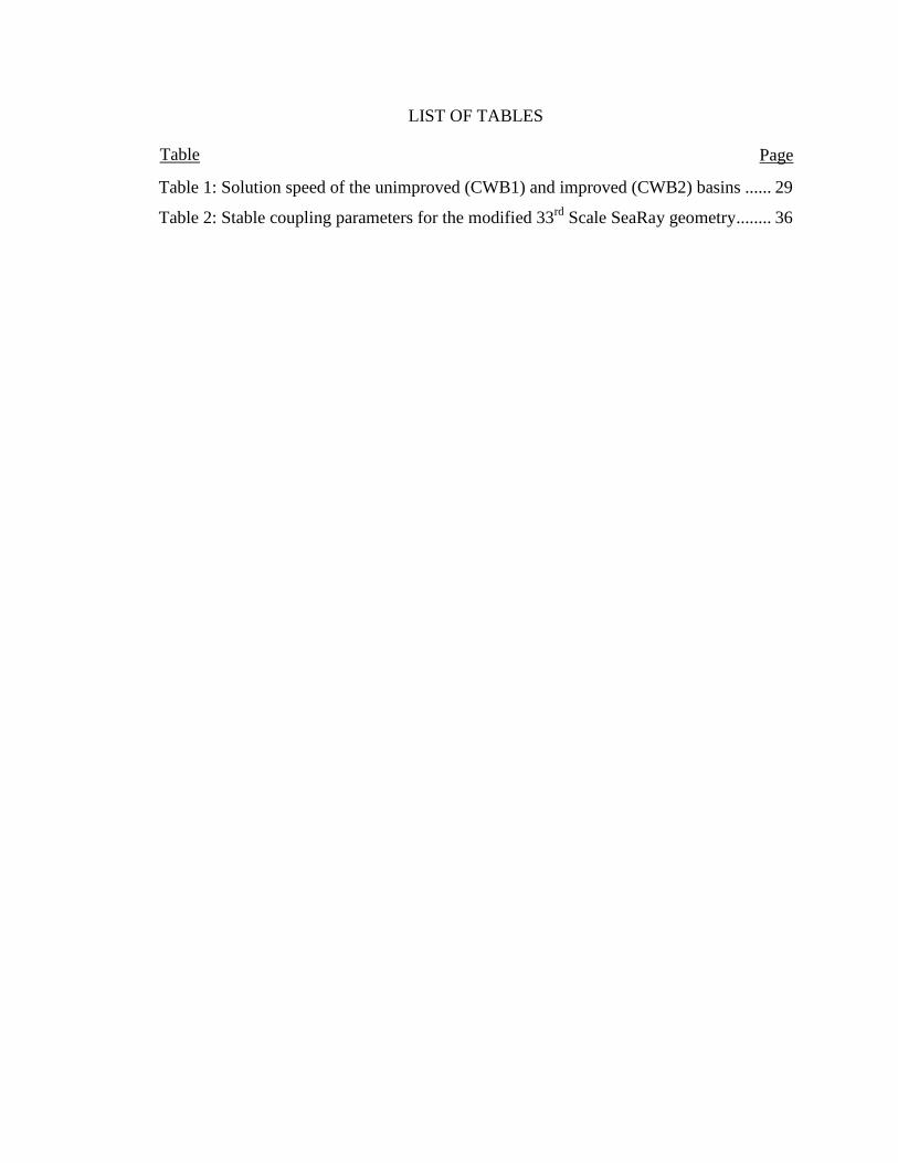
Table 1: Solution speed of the unimproved (CWB1) and improved (CWB2) basins ...... 29
Table 2: Stable coupling parameters for the modified 33rd
Scale SeaRay geometry ........ 36
Page Table
LIST OF APPENDICES
Appendix A - Strain Gage Selection, Installation, and Protection ................................... 49
A1. – Strain Gage Selection - Composite Hull Installations ...................................... 49
A.2 – Strain Gage Selection – End Stops ................................................................... 50
A.3 – Strain Gage Installation ..................................................................................... 51
A.4 – Strain Gage Protection ...................................................................................... 51
Appendix B – ALE / Lagrange Fluid Coupling and Leakage Prevention ........................ 54
B.1 – Definition of the Initial Volume Fraction ......................................................... 54
B.2 –Constrained Lagrange in Solid ........................................................................... 57
B.3 – The *Constrained_Lagrange_in_Solid Card ..................................................... 57
B.4 – Fluid Coupling................................................................................................... 59
B.5 – Good Modeling Practices .................................................................................. 63
B.6 – Tricks of the Trade ............................................................................................ 64
Appendix C – Fast Gravity Application in LS-DYNA ..................................................... 66
Appendix D – Mooring Lines, Implementation of Cable Elements ................................. 68
D.1 – Creating Beam Elements ................................................................................... 68
D.2 – Defining the Loading Curve ............................................................................. 68
D.3 – Creating the Stress-Strain Load Curve.............................................................. 69
Appendix E - Rotational Damping ................................................................................... 72
E.1 – Creating a Revolute Joint .................................................................................. 72
E.2 – Applying Damping to the Joint ......................................................................... 73
E.3 – Plotting Joint Force and Moments ..................................................................... 75
Appendix F – Writing, Extracting, and Plotting LS-DYNA Result Files ........................ 76
F.1 – Writing and Extracting ...................................................................................... 76
F.2 – Plotting FSI Forces ............................................................................................ 77
Page Appendix
LIST OF APPENDIX FIGURES
Figure 21: Protective layers on a strain gage subject to immersion in seawater. ............. 52
Figure 22: The first tier of the IVF card ........................................................................... 54
Figure 23: The second tier of the *IVFG card .................................................................. 55
Figure 24: Misaligned /coarse meshes cause the IVF card trouble. ................................. 56
Figure 25: Properly aligning meshes results in a well-fit IVF result ................................ 56
Figure 26: *CLiS card, which defines contact between ALE and Lagrange elements ..... 58
Figure 27: WEC geometry with separate ALE domains for the air inside the bodies. ..... 60
Figure 28: Initial volume fraction card for multi-body coupling ...................................... 61
Figure 29: Fluid coupling of the body to the domain water and air ................................. 62
Figure 30: Fluid coupling of the body with the air inside................................................. 63
Figure 31: WEC geometry needing separately defined stiffnesses .................................. 64
Figure 32: WEC geometry with boxes defining two separate coupling sets .................... 65
Figure 33: Pressure oscillations resulting from gravitational jerk .................................... 67
Figure 34: Damping curve for ALE water elements ......................................................... 67
Figure 35: *Mat_071-Cable_Discrete_Beam input deck ................................................. 69
Figure 36: *Section_beam input deck............................................................................... 69
Figure 37: Layout of the joint used in *Constrained_joint_revolute. ............................... 72
Figure 38: *Constrained_joint_stiffness_generalized input deck ..................................... 74
Figure 39: Card 2 of the *Constrained_joint_stiffness_generalized input deck ............... 74
Figure 40: Plotting the joint forces using the JStiffR button. ........................................... 75
Figure 41: LS-PrePost GUI with locations used for extracting ACSII binout files.......... 77
Figure 42: *Dbase_FSI card with parts selected for output .............................................. 78
Page Figure
Hydroelastic Modeling of a Wave Energy Converter
Using the Arbitrary Lagrangian-Eulerian
Finite Element Method in LS-DYNA
1. Introduction
Ocean wave energy is a new and promising form of renewable energy in which wave
energy converters (WECs) harness energy from passing ocean waves, and convert it into
useable electrical energy. WECs are usually deployed more than 3 km offshore, where
the energy in the ocean waves arrives as a result of far off wind and storms largely
undiminished. Across the world, there is a great amount of research being conducted to
help develop, test, and deploy these devices [1]; however the industry is still in its
infancy. Some full scale, grid connected devices have been deployed, but widespread
commercial production is still a few years off.
Most of the current research in the field is being conducted in the areas of numerical
modeling, power production estimation, array modeling, and device reliability and
survivability. Traditionally, to model the hydrodynamic response of their device, wave
energy developers have applied frequency-domain techniques developed by other
offshore industries. Most modeling efforts to date have been focused in the frequency-
domain, utilizing linear approximations to determine device responses to monochromatic
waves and unidirectional wave spectra. More recently, work has been conducted in the
time domain using convolved frequency-domain data; however, many of the same pitfalls
of frequency-domain analysis remain. While this approach has been proven accurate in
quasi-static applications the offshore oil and gas industry, it has become apparent that this
approach is not necessarily the best for wave energy conversion.
Under the assumptions of potential flow; inviscid, irrotational fluids, and low amplitude
motions, significant discrepancies can occur between simulation results and reality.
Many WECs are designed to operate at or near resonance in order to extract the most
energy through the relative oscillation of two or more bodies at or near the natural
frequency of the passing waves. During this type of operation, the assumptions of
2
potential flow deteriorate, and errors can become especially high. In addition, general
purpose potential flow codes often only account for first order (i.e. linear) waves, which
means other conditions of interest such as fetch limited, higher-order, steep or breaking
waves cannot be accounted for.
One of the main challenges toward the development of WECs is reliability and
survivability of devices in the open ocean, and with recent disasters including the
Macondo well explosion and ensuing oil spill in the Gulf of Mexico, tsunamis in the
Pacific, and increasingly severe and erratic weather patterns, more attention than ever is
being devoted to this topic. To overcome some of the current limitations of numerical
modeling of offshore structures, we seek an alternative method, which can more
accurately estimate the hydroelastic response of a WEC. A finite element approach to
marine hydrodynamics is particularly of interest to wave energy developers because of its
inherent ability to assess the safety of WECs in both day-to-day (operational sea)
conditions and extreme (high sea state) events.
With the finite element method, loading on device components such as joints, mooring
lines and terminations, hull panels, and many other components of interest can be
resolved in the time-domain. In many frequency-domain numerical models, the ability to
model linear mooring forces exists; however, this approach does not fully model the
device dynamics. Since the response amplitude operators (RAOs) for the floating body
are calculated in the absence of mooring forcing, the simulation must solve for the total
system RAOs by adding the linearized terms during post-processing.
The time-domain analysis technique of the finite element approach ensures that external
forcing such as mooring lines and power take-off are coupled to the structure at each
timestep; on the order of 10-4
to 10-6
seconds for explicit models. The result is fully-
coupled, fully-nonlinear structural response in the time-domain. This approach is capable
of modeling structural elasticity, nonlinear power take-off forcing, viscous effects and
vorticity of the water, and other parameters which can only be linearly approximated in
frequency-domain modeling. The finite element approach opens the door to the
3
possibility of conducting fatigue studies and determining failure criteria for critical
components. The capability also exists to model higher order and steep waves, as well as
extreme events such as breaking waves, 100 year waves, and ship collisions which are of
great interest and importance.
The extended capability of the finite element approach makes it attractive to wave energy
developers and ocean structural engineers, but its application towards fluid-structure
interaction (FSI) has not been fully assessed for WECs in this type of long-duration
contact problem. For these reasons, this study seeks to assess the applicability of LS-
DYNA in modeling WEC hydroelasticity.
The current version of LS-DYNA is an explicit multi-physics nonlinear finite element
code developed by John O. Halquist and LSTC. Among other solution techniques, the
program uses an Arbitrary Lagrangian Eulerian (ALE) formulation and a compressible
Navier-Stokes solver to determine body forces as a result of fluid-structure interaction
(FSI). FSI in LS-DYNA has been studied and verified extensively since its first
introduction in version 940 in 1996. Numerous papers have been published for short-
duration problems through LS-DYNA user conferences[2-8], as well as through outside
journals and conferences [9-11]. The papers listed above are but a small fraction of the
overall published material, but should serve as a suitable starting point for available
literature on this topic.
Although the contact algorithm and ALE formulation is well proven, most of its
application to date has been in short-duration contact and impact problems such as blast
loading, airbag simulations, car crashes, and metal forming to name a few. With regards
to ocean engineering, only a few studies have been published using the FSI capability in
LS-DYNA to study water impacts on bottom fixed structures, breakwaters, and ship hulls
[12-14]. In the case of a WEC, we are interested in long-duration scenarios where waves
impact floating, moored bodies. At present, to the author‟s knowledge, the longest
published contact duration using ALE FSI is 14 seconds [12], and to date, no studies on
floating structures have been published with this method.
4
This study is part of a larger effort to assess the application of LS-DYNA towards
modeling structural hydroelasticity, with the hope of demonstrating the applicability of a
new finite element based methodology in modeling WECs. This document presents the
initial work towards numerical modeling and verification of the Columbia Power
Technologies SeaRay WEC using the FSI capability of LS-DYNA. The following
section of the document will first cover a brief background of the development of the
SeaRay concept, testing conducted to date, and detail the data available for verification of
numerical results. The third section presents the LS-DYNA simulation environment,
including details on the ALE element formulation and the compressible Navier-Stokes
solver. Consideration is also given to Lagrangian-ALE coupling and numerical stability.
The fourth section presents improvements the computational wave basin which
significantly decreases overall computation time in increases numerical accuracy of the
computational domain. The fifth section details the construction of the SeaRay and other
WEC component models using LS-PrePost. This section also sheds light on the current
capabilities of the software with special attention to realistic mooring, and simulation of
power take-off (PTO) control using user defined implicit functions. The sixth section
shows the results of initial modeling efforts, including quantification of the benefits of the
improved computational wave basin, a quasi-static mooring analysis of the 7th
scale
SeaRay, and FSI studies for the 33rd
scale SeaRay. The final section presents the
conclusions of this study and future works.

5
2. Project Background
This section begins with a short history of the development of the SeaRay WEC concept,
and summarizes scaled testing conducted to date. Experimental setup and
instrumentation of the scaled tests on the SeaRay in the wave tank and the open ocean are
discussed, and suggestions are made concerning the usage of experimental data in
numerical model validation.
2.1 – Research and Development of the SeaRay Concept
Development of linear direct-drive (LDD) WEC technology began at Oregon State
University in 2005 under Dr. Annette von Jouanne and the late Dr. Alan Wallace. Initial
efforts focused on LDD generators for point absorbing WECs [15-17]. Oregon State
conducted an ocean deployment of their first-generation LDD device called “SeaBeav1”
off the coast of Newport, Oregon in 2007 [18]. The following year, Columbia Power
Technologies and OSU jointly deployed a second generation 10 kW LDD device in the
same location [19].
In 2008, Columbia Power Technologies began developing a rotary direct drive device
called the SeaRay. The SeaRay is classified as a point absorbing WEC, but as opposed to
other well known point absorber designs, it harnesses energy from the rotational motion
of the floats, as opposed to linear motion. As a wave passes the structure, the reaction
plate located at the bottom of the spar acts to keep the central member relatively
stationary, while the floats are allowed to rotate relative to the nacelle. As the floats
rotate, they turn a direct drive PTO system which produces electrical power. The power
is smoothed onboard, and sent back to shore via an underwater cable.
The SeaRay was first tested at 33rd
scale in Oregon State‟s Hinsdale Wave Research
Laboratory (HWRL) Directional Wave Basin (also known as the Tsunami Basin) in
2009, and then again at 15th
scale in the Hinsdale long wave flume in 2010 [20]. A
picture of the 15th
scale device fitted with LED wands for body tracking with Phase

6
Space is shown in Figure 1. Using data taken from the tank testing, they were able to
validate their previous numerical simulations which were conducted using ANSYS
AQWA, a commercially available potential flow code. Numerical modeling was
conducted with the buoy at full scale, and then the response was Froude-scaled down for
comparison with tank testing results. Good agreement was achieved by iteratively
modifying a viscous damping term available within the software until the RAOs of
experimental and simulation data matched satisfactorily. This term is not a physical
parameter, but rather attempts to provide an approximation of viscous effects which
occur due to the buoy‟s motion by applying additional structural damping.
Figure 1: Columbia Power Technologies' 15th
scale SeaRay during tank testing
In 2010, a shape optimization study of the SeaRay concept was conducted, and a new
design for the buoy structure was devised which increases the hydrodynamic efficiency
of the device [21]. Subsequently, the new shape was tested at 33rd
scale in the OSU
HWRL Directional Basin in early 2011. Tank testing was conducted for a single device,
as well as for several different array configurations using up to five 33rd
scale SeaRay
buoys [22]. Six-DOF buoy motions were again captured using Phase Space, and passive
rotational damping was applied to the floats by a dashpot to simulate PTO forcing. From
7
the 33rd
scale basin tests, acceleration, velocity and position are available for each body.
Instantaneous position and speed of the PTO, and measured wave heights from the basin
are also available for validation purposes.
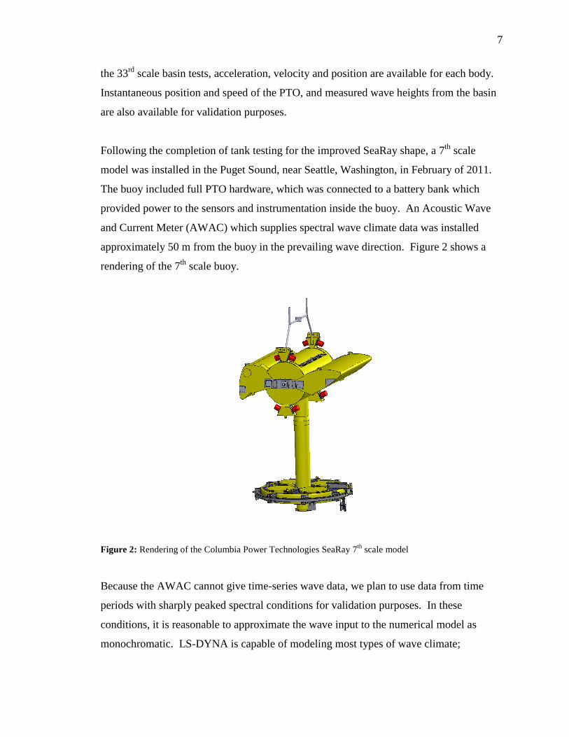
Following the completion of tank testing for the improved SeaRay shape, a 7th
scale
model was installed in the Puget Sound, near Seattle, Washington, in February of 2011.
The buoy included full PTO hardware, which was connected to a battery bank which
provided power to the sensors and instrumentation inside the buoy. An Acoustic Wave
and Current Meter (AWAC) which supplies spectral wave climate data was installed
approximately 50 m from the buoy in the prevailing wave direction. Figure 2 shows a
rendering of the 7th
scale buoy.
Figure 2: Rendering of the Columbia Power Technologies SeaRay 7th
scale model
Because the AWAC cannot give time-series wave data, we plan to use data from time
periods with sharply peaked spectral conditions for validation purposes. In these
conditions, it is reasonable to approximate the wave input to the numerical model as
monochromatic. LS-DYNA is capable of modeling most types of wave climate;
8
however, initial numerical studies should be conducted with regular waves to simplify the
simulation.
The buoy was fitted with a 6-axis accelerometer in the nacelle of the device. To
supplement the determination of position determined by the accelerometer, a GPS unit
was also used to determine heading and drift from the mean installed position. Shackle
load cells were attached to all three mooring connection points, which are located at even
intervals on the outside of the reaction plate. Encoder data is available for the float
rotations. Data from the buoy was wirelessly transmitted to shore. Additionally, the
device was fitted with 16 channels of strain gages, which is covered in the next section.
2.2 – Strain and Force Transducers
In addition to the sensors mentioned above, six channels of biaxial rosette gages were
installed on the hull of the nacelle. In the future, data from these sensors will help to
verify the coupled hydrodynamic and elastic response of the hull structure. Two uniaxial
gages were installed inside the spar, on the forward and aft walls, approximately one
meter from the nacelle joint. One biaxial rosette was installed on each side of the nacelle
walls, approximately 0.5 m above the top of the PTO frame. The purpose of these gages
was to monitor the strain as a result of PTO torque. Another objective of the starboard
and port rosettes was to determine the stresses caused by large ship wakes hitting the
WEC at oblique angles. The third rosette was installed in the center of the forward wall
with respect to the lateral and vertical directions. This gage was placed at a location
where maximum expected stress from combined wave slapping and bending due to PTO
forcing would occur.
The central body of the SeaRay was manufactured in two main pieces; the top portion
containing the nacelle and upper spar section, and the bottom portion containing the
lower spar and the reaction plate. Two uniaxial strain gages were installed on the
forward and aft walls above the connection joint for the upper and lower spar sections.
The gages were located such that they were positioned sufficiently far away from
9
connections and joints in order to avoid stress concentrations. The installation location
was 570 mm from the nacelle/spar interface joint.
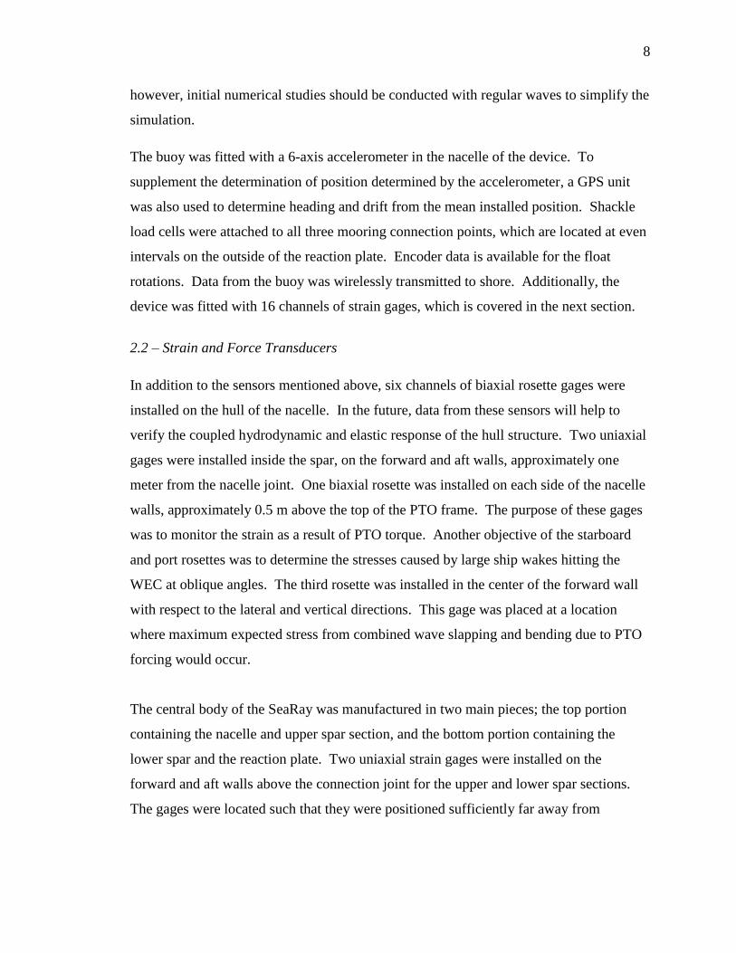
Figure 3 shows a representative data set from the spar strain gages. From this set, we see
what we would expect with input from a unidirectional wave spectrum which is typical of
the Puget Sound test site. The reaction in the two gages is approximately equal and
opposite, as is expected with the spar in bending. The strain pattern follows what might
be expected as a wave group passes the WEC, with minimum strain as the wave packet
arrives at the WEC, and a maximum as one half of the packet has passed. A slight tensile
offset of about 15 µɛ is observed, which could be attributed to ocean currents at the site,
Stoke‟s drift wave forces, or thermal drift in the signal conditioner.
Figure 3: Sample data set from strain gages located in the upper spar of the 7th
scale SeaRay
An additional 8 channels of strain gages were installed on the outside of the hull to
monitor float slam loads. The control systems of the PTO were designed such that the
maximum rotation of the floats was limited to 45 degrees. This was achieved by
increasing the damping on the floats by increasing the resistive load on the generators. In
the event that an excessive amount of torque was detected on the output shaft, a ratchet
mechanism would allow the float to freewheel in order to avoid damage to PTO
components. Although it was unlikely that this event would occur, the structure was
10
instrumented with strain gages in order to determine the structural loading in the event
that the float impacted the end stops.
Galvi RMV160.160 end stops were used for this application, which are designed to
withstand impacts of up to 70 kN. The bumpers are made of chambered polyurethane
fixed to a thick aluminum back plate, and are designed to absorb compressive impacts at
speeds up to 4 m/s by deforming up to 75% of their original height. End stops were
mounted in 8 places on the outer hull, on the top and bottom of the nacelle, as can be seen
in Figure 2.
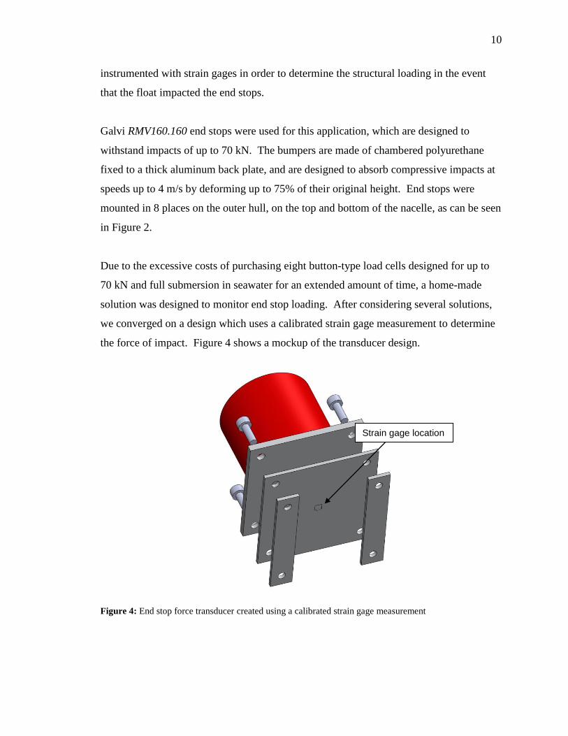
Due to the excessive costs of purchasing eight button-type load cells designed for up to
70 kN and full submersion in seawater for an extended amount of time, a home-made
solution was designed to monitor end stop loading. After considering several solutions,
we converged on a design which uses a calibrated strain gage measurement to determine
the force of impact. Figure 4 shows a mockup of the transducer design.
Figure 4: End stop force transducer created using a calibrated strain gage measurement
Strain gage location

11
Since eight of these transducers needed to be machined, instrumented, and installed, it
was important to keep the design as simple as possible to reduce manufacturing cost and
installation time. Each transducer required three pieces of machined 6.35mm (0.25”)
6061 aluminum sheet. The square back plate was instrumented with a single strain gage
oriented in the transverse direction (grid aligned perpendicular to the standoff strips), in
order to obtain the highest output due to the bending of the plate as load was applied to
the bumper. The choice of thickness of the plate allows for maximum sensitivity of the
strain gage at low impacts, and ensures that the metal does not yield at an impact of 70
kN. The two narrow strips bolted between the hull and the back plate serve as spacers
that allow room for plate bending during impact and additional surface coatings to protect
the gage from the harsh seawater environment.
Once the strain gages were applied to the underside of the back plate, the whole assembly
loaded in compression on an Instron machine. Each bolt was tightened to specification
using a torque wrench in order to ensure uniformity between each assembly. Strain
readings were recorded for eight compressive loads from 1 to 70 kN. A plot the
calibrated response of all eight end stop channels can be seen in Figure 5.
Figure 5: Strain versus compressive loading force for all eight end stop channels
After each assembly was calibrated, onboard signal processing software was programmed
to determine an end stop strike by the magnitude of the strain gage response, and to
12
record the strike duration and magnitude in a separate file for future analysis. To prevent
the system from recording false impacts resulting from thermal drift, the end stop voltage
was re-zeroed every one minute. This was necessary due to the extreme temperature
changes that a strain gage located above the waterline could experience if splashed by
frigid seawater on a hot day. The entire assembly was bolted onto the WEC hull using
four stainless steel bolts at each corner, torqued to the same specification used in the
calibration.
A custom designed signal conditioner with 16 channels of quarter bridge circuits was
used to monitor strain signals. The conditioner was designed with an excitation voltage
of 2.5 V, and output 0 to 5 V. A low excitation voltage was used to decrease resistive
heating by the gage grid. Since low strain ranges were expected during the WEC‟s
operation, the bridge completion resistors for the strain gages installed inside the buoy
were chosen to be 1 ppm/°C high precision resistors. The high thermal tolerance lowers
the susceptibility of the signal conditioning system to thermal drift. The channels
receiving signals from the end stops utilized 5 ppm/°C resistors, because of the high
thermal conductivity of the aluminum back plate. A three wire connection was used for
all gage leads to further reduce the possibility of thermal drift. For 2 m of three-wire
lead, the worst-case thermal drift was determined to be 1.9 µɛ/°C and 7.5 µɛ /°C for the 1
ppm/°C and 5 ppm/°C circuits, respectively.
All strain gages and their wires were treated extensively with a series of protective
coatings to protect them from damage caused by extended immersion in seawater, or
contact with salt air. Details of the choice of hardware, materials used for protection, and
the process of application can be found in Appendix I.
13
3. Modeling in LS-DYNA
This section will introduce the LS-DYNA simulation environment. The first subsection
will detail the LS-DYNA governing equations and element formulations used in this
study. The second subsection will discuss the contact algorithm used to couple the ALE
water elements with the Lagrangian shell elements of the buoy structure. The final two
subsections will introduce the design and implementation of computational wave basins
(CWBs) used in the analysis of floating structures.
3.1 – ALE Formulation and Fluid Solver
LS-DYNA is a multi-physics finite element code designed for use in highly non-linear
problems. The program is capable of solving solid and fluid mechanics, as well as heat
transfer. LS-DYNA is used for a wide array of problems, including sheet metal forming,
impact and crash simulations, explosions, and fluid-structure interaction by many
different industries.
In this study, the ALE fluid formulation coupled with Lagrangian solid is used to study
FSI. The ALE fluid formulation is of particular use for this type of experiment, because
it is capable capturing the nonlinear effects of vorticity and viscosity. The ALE
formulation combines the benefits of Lagrangian elements which are typically used in
classical mechanics with Eulerian elements which can accurately track fluid particle
movements. The LS-DYNA multi-material formulation employs a Lagrangian timestep,
followed by a “remap” or “advection” step. During the advection step, the nodes of the
ALE element are moved in either a Lagrangian or Eulerian manner, or an arbitrary
combination of the two, in order to smooth the mesh distortion which occurred during the
previous timestep. Smoothing the mesh helps to avoid erroneous results which can arise
in highly distorted elements. The Van Leer + half index shift advection algorithm used in
this study, which is second-order accurate [23,24].
14
After the mesh has been smoothed, internal energy, nodal velocities and momentum from
the last timestep are re-mapped to the smoothed mesh. In the simulations conducted in
this study, the number of remap operations per timestep was chosen to be unity, as the
computational cost of the advection process is very high. More detailed information on
the ALE formulation and smoothing algorithms can be found in the LS-DYNA Theory
manual [25].
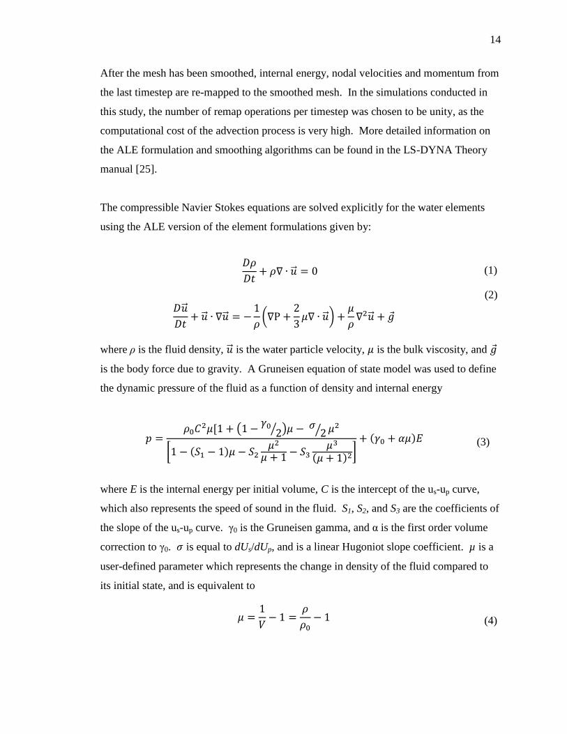
The compressible Navier Stokes equations are solved explicitly for the water elements
using the ALE version of the element formulations given by:
(1)
(2)
where ρ is the fluid density, is the water particle velocity, is the bulk viscosity, and
is the body force due to gravity. A Gruneisen equation of state model was used to define
the dynamic pressure of the fluid as a function of density and internal energy
(3)
where E is the internal energy per initial volume, C is the intercept of the us-up curve,
which also represents the speed of sound in the fluid. S1, S2, and S3 are the coefficients of
the slope of the us-up curve. γ0 is the Gruneisen gamma, and α is the first order volume
correction to γ0. is equal to dUs/dUp, and is a linear Hugoniot slope coefficient. µ is a
user-defined parameter which represents the change in density of the fluid compared to
its initial state, and is equivalent to
(4)
15
where ρ0 is the initial density, and ρ is the density of the fluid at the current time step.
The sound speed in water was set to 150 m/s, and S1 and γ0 are set to 1.979 and 1.4,
respectively, as suggested by Zhang and Yim [12]. S2 and S3 are set to zero, as they
apply to compressed gasses, which are not included in this model.
With the current formulation, the model accounts for viscosity of the fluid. Viscous
effects of the water on the structural elements are approximated by the equation of state
model. Since the mesh resolution at the fluid-structure interface is many orders of
magnitude larger than the width of the boundary layer, the solver estimates viscous drag
by interpolating the shear stress over the elements lying at the fluid-structure interface.
Accurate resolution is especially important for small structures such as the 33rd
scale
SeaRay because the magnitude of the drag force is contributes significantly to the overall
force on the body. For a full scale WEC, viscous effects may not be as important.
3.2 – ALE Coupling and the Structural Solver
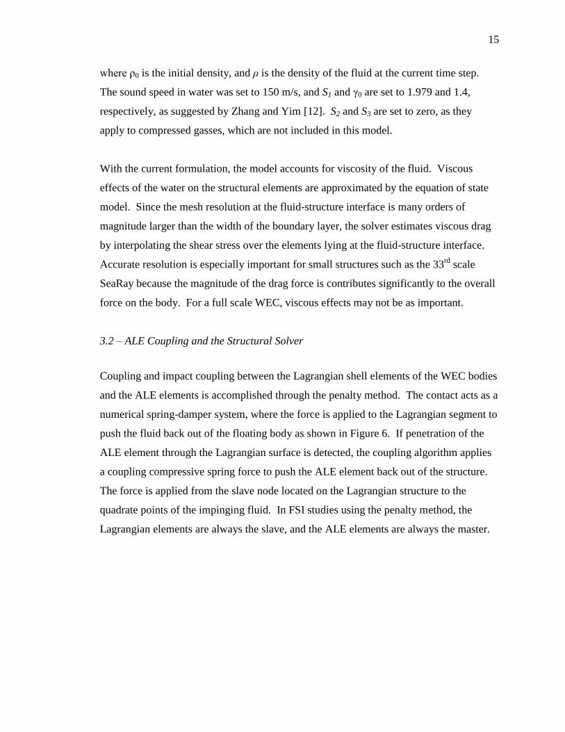
Coupling and impact coupling between the Lagrangian shell elements of the WEC bodies
and the ALE elements is accomplished through the penalty method. The contact acts as a
numerical spring-damper system, where the force is applied to the Lagrangian segment to
push the fluid back out of the floating body as shown in Figure 6. If penetration of the
ALE element through the Lagrangian surface is detected, the coupling algorithm applies
a coupling compressive spring force to push the ALE element back out of the structure.
The force is applied from the slave node located on the Lagrangian structure to the
quadrate points of the impinging fluid. In FSI studies using the penalty method, the
Lagrangian elements are always the slave, and the ALE elements are always the master.

16
Figure 6: Visualization of the fluid coupling spring force
The compressive spring force on is defined as F = -kd, where d is the penetration
distance, and k is the estimated critical stiffness, given by
(5)
where fsi is the user-supplied scale factor for the interface stiffness, Ki is the material bulk
modulus, and Ai is the shell element face area. In the event that the maximum penetration
is exceeded during a timestep, supplemental leakage control is applied in the same
manner as the primary leakage control, which supplies an additional coupling force
proportional to the estimated critical stiffness. This additional leakage control can be
thought of as a second spring added in parallel. Use of coupling damping is not
necessary, but it has been observed that a damping factor of 90% of critical acts to reduce
numerical noise.
Determination of the correct coupling stiffness is a difficult task, and is still an active area
of research [26]. The coupling parameters must be chosen with care, as spring with
excessive stiffness can artificially alter the ALE element velocity, while a spring which is
too weak will not adequately prevent leakage. It has been shown that the solutions of FSI
simulations using this method are highly dependent on the contact stiffness in relation to
the mesh density, so obtaining accurate stiffness parameters is paramount to successful
modeling [27]. In this study, the correct coupling force was determined iteratively by
ramping up the stiffness until an acceptable level of stability was achieved. More
Structure
Fluid
k
d
Nodes
17
information on stability and coupling parameters can be found in the results section of
this document.
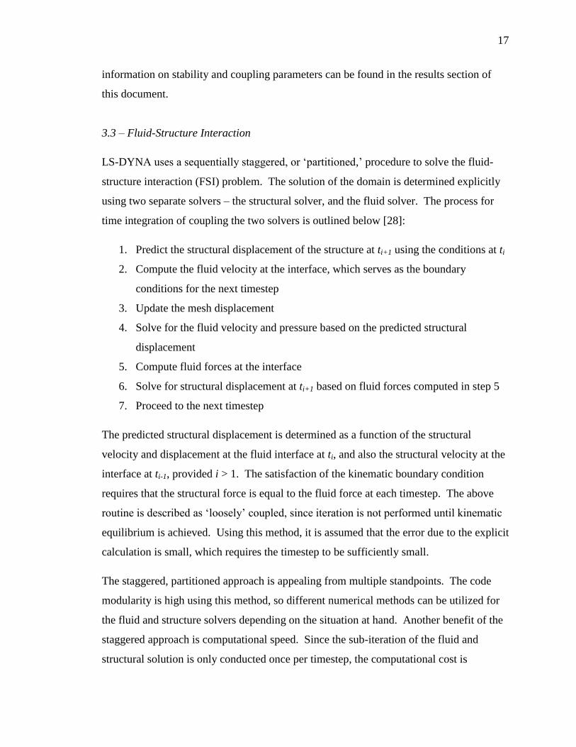
3.3 – Fluid-Structure Interaction
LS-DYNA uses a sequentially staggered, or „partitioned,‟ procedure to solve the fluid-
structure interaction (FSI) problem. The solution of the domain is determined explicitly
using two separate solvers – the structural solver, and the fluid solver. The process for
time integration of coupling the two solvers is outlined below [28]:
1. Predict the structural displacement of the structure at ti+1 using the conditions at ti
2. Compute the fluid velocity at the interface, which serves as the boundary
conditions for the next timestep
3. Update the mesh displacement
4. Solve for the fluid velocity and pressure based on the predicted structural
displacement
5. Compute fluid forces at the interface
6. Solve for structural displacement at ti+1 based on fluid forces computed in step 5
7. Proceed to the next timestep
The predicted structural displacement is determined as a function of the structural
velocity and displacement at the fluid interface at ti, and also the structural velocity at the
interface at ti-1, provided i > 1. The satisfaction of the kinematic boundary condition
requires that the structural force is equal to the fluid force at each timestep. The above
routine is described as „loosely‟ coupled, since iteration is not performed until kinematic
equilibrium is achieved. Using this method, it is assumed that the error due to the explicit
calculation is small, which requires the timestep to be sufficiently small.
The staggered, partitioned approach is appealing from multiple standpoints. The code
modularity is high using this method, so different numerical methods can be utilized for
the fluid and structure solvers depending on the situation at hand. Another benefit of the
staggered approach is computational speed. Since the sub-iteration of the fluid and
structural solution is only conducted once per timestep, the computational cost is

18
comparatively low. Speed is also increased by the fact that the fluid and structural
meshes are completely decoupled. As compared to a „monolithic‟ algorithm which
constructs one global stiffness matrix for all of the fluid and structural elements in the
domain, the partitioned approach utilizes separate stiffness matrices for the fluid and
structure, joined using one or more smaller coupling matrices. Since the matrices of the
partitioned approach are smaller than in a monolithic simulation of the same number of
elements, the solution of the elemental stresses at each timestep is much faster.
3.4 – Multi-Body Coupling Definitions in LS-DYNA
In fixed structures, correct coupling can be achieved even with water elements
overlapping or filling the structure, as long as the ALE elements do not penetrate through
the structure surface. For instance, in the study by Tokura and Ida [29], the bottom fixed
barrier was filled with water. Due to the presence of fluid on the inside of the barrier, the
coupling stability was inherently more stable, since the fluid pressures on either side of
the shell element were equal. With this advantage of pressure equilibrium and short
simulation time, determination of the coupling stiffness is less complicated, and a smaller
coupling stiffness can be used to prevent the penetration of the water elements lying
outside the barrier.
With a (movable) floating structure, the situation is more complicated. The coupling
relationship is especially important because of the vast difference in pressure between the
fluids on either side of the structure. In this case, the hydrostatic stiffness of the WEC is
defined by the amount of water it displaces, so the inside of the structure which lies
below the still water level must be evacuated of water and filled with air. This is
accomplished through the *Initial_Volume_Fraction card, which performs a series of
filling and emptying actions. The card is used to remove any water elements initially
lying inside the structure and fills the void with a new ALE air part. A detailed
explanation of the filling and initialization process is available from Aquelet, Seddon,
Souli, and Moatamedi [30].

19
The definition of the coupling relation between the three ALE parts and the floating
structure is very important when considering numerical stability. Without the correct
overall definitions for coupling, stability for any appreciable amount of time will be
difficult or impossible to achieve, even if the correct parameters for the coupling stiffness
are known. Through trial and error, it was determined that coupling must be defined
separately for each ALE-structure pair.
For example, consider the floating three-body WEC shown in Figure 7. From the figure,
we see five ALE parts; domain air and domain water as light brown and red wire on the
edges of their respective boundaries, and air inside the WEC bodies as yellow, light blue
and green. The shell normals for all three bodies point outward into the domain ALE
elements. The correct coupling for this body is achieved by coupling both the domain
water and air elements to the outer body surface. Since we want not only to prevent
water from leaking in, but also to prevent air from leaking out, the inside air must be
coupled to body. Coupling of the air elements inside the bodies was accomplished by
changing the shell normal definition to the “left hand rule.” This alerts the coupling
algorithm to conduct a slave search for the air elements lying on the inside of the shell.
All coupling definitions were in the compressive direction only, as this is the nature of
the interaction.
Figure 7: Simple floating case for WEC geometry with three separate ALE parts
20
4. Computational Wave Basin Improvements
This section will introduce the improvements to the computational wave basin (CWB).
The first subsection introduces the composition of the unimproved basin, while the
second subsection details the modifications that were implemented in order to decrease
computational requirements. Studies which quantify the speed increase and other
benefits of the improved CWB can be found in Section 6 of this report.
4.1 – General Computational Basin Construction
In this study, two different types of CWBs were used. The first type of basin is
cylindrical in shape, and was used to conduct short numerical studies when attempting to
determine the correct coupling stiffness parameters. This basin consists of two parts, air
and water, with the nodes lying on the outer boundaries fixed in all 6-DOF. The round
shape of the basin reduces instability caused by „corner effects‟ which appear in smaller
rectangular basins as a result of surface and/or acoustic waves being focused into the
corners of the basin. These basins were designed on a case-by-case basis such that their
dimensions were as small as possible to reduce computation time. The smaller number of
elements in the cylindrical basins made it much more efficient to conduct a large number
of short numerical studies. As a rule of thumb, the basin width and depth should be about
twice that of the part in consideration.
The second type of basin used in this study is the numerical wave tank. A generic layout
of a wave basin is shown below in Figure 8. The shell wavemaker (green) is located at
least twice the maximum stroke from the rear boundary. Regular waves were created by
sinusoidally oscillating the wavemaker with a stroke of H/kh, where H is the wave height,
k is the wave number, and h is the water depth. The water is coupled to the wavemaker
in both compression and tension, and the nodes at the paddle surface are not merged to
allow the water to „slip‟ on the surface.

21
Figure 8: Sample layout of an unimproved computational wave basin
Two boundary conditions govern the simulation of the numerical wave tank. The first
condition constrains the motion of the nodes of the ALE elements which are located on
the boundary of the basin. The nodes located on the corners of the CWB are constrained
in the three principal translational directions, while the nodes on the edges of the basin
were constrained in two dimensions. A “free-slip” boundary condition (constrained in
the normal direction) was applied to the nodes lying on the walls of the basin.
The second set of boundary conditions are applied at the interfaces between the ALE
elements and the structural shell elements of the wavemaker and the floating structure.
The kinematic constraint is that no fluid particles can pass through the Lagrangian
interfaces. The dynamic constraint is that the stress must be continuous across the
surfaces – that is to say that the pressures of an ALE and Lagrangian element in contact
should be equivalent.
The ALE water and air elements consist of 8-node solid 1-point ALE elements, with
increased mesh density near the structure of interest. The mesh sizes of the elements are
dependent on the specific model and flow characteristics, but for 33rd
scale simulations,
the element size at the wavemaker should be from 100 to 125mm, and the mesh should
increase in density in the vicinity of the structure. A good starting mesh size near the
structure was determined to be 25 mm. The water elements were modeled using null

22
material with a density of 1x10⁻⁹
ton/mm3 and dynamic viscosity of 1.08x10
-9 MPa/s.
The air elements were modeled with elements at zero pressure and density. The nodes
shared by the air and the water are merged so that the free surface can be effectively
resolved.
4.2 – CWB Improvements
The first improvement to the basin reduces the computational resources needed to
generate waves, and brings the waves in a basin to a steady state more quickly. In
previous experiments with water waves in LS-DYNA, piston-type wavemakers were
modeled with rigid shell elements as shown in Figure 8. This additional fluid-structure
interaction unnecessarily increases the computation time required for the simulation due
to the costly coupling of the fluid to the Lagrangian elements. In order to reduce the time
required to complete a simulation, waves were created by prescribing the nodal velocities
of the ALE elements at the inflow boundary. The velocities for monochromatic waves in
the horizontal and vertical directions are taken to be
(6)
(7)
where g is the acceleration due to gravity, x and z are the nodal locations in the horizontal
and vertical directions, respectively, and is a phase term equal to 2π divided by the
wave period [31].
To further reduce the time needed for the basin and oscillating bodies to reach a steady
state response, nodal velocities of the water elements were prescribed in the vertical and
downstream directions. To increase the stability of the simulation, initial conditions were
only prescribed for every other set of nodes in the vertical and downstream direction.
Within 2 characteristic widths of the buoy or structure, no nodal velocities were
23
prescribed. The initial conditions of the wave particle velocities continued for two wave
periods, until a well defined wave had formed in the basin. For the rest of the simulation,
the prescribed velocity at the inflow boundary acted as the wave generation source.
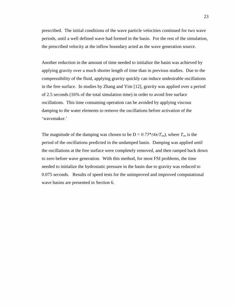
Another reduction in the amount of time needed to initialize the basin was achieved by
applying gravity over a much shorter length of time than in previous studies. Due to the
compressibility of the fluid, applying gravity quickly can induce undesirable oscillations
in the free surface. In studies by Zhang and Yim [12], gravity was applied over a period
of 2.5 seconds (16% of the total simulation time) in order to avoid free surface
oscillations. This time consuming operation can be avoided by applying viscous
damping to the water elements to remove the oscillations before activation of the
„wavemaker.‟
The magnitude of the damping was chosen to be D = 0.75*(4π/Tos), where Tos is the
period of the oscillations predicted in the undamped basin. Damping was applied until
the oscillations at the free surface were completely removed, and then ramped back down
to zero before wave generation. With this method, for most FSI problems, the time
needed to initialize the hydrostatic pressure in the basin due to gravity was reduced to
0.075 seconds. Results of speed tests for the unimproved and improved computational
wave basins are presented in Section 6.
24
5. WEC Component Modeling
This section will cover the construction and modeling of the three main WEC
components; the structural hull model, the power take-off, and the mooring system. The
results of the integration of all of these components into a computational wave basin
fluid-structure interaction model will be introduced in the following section of this report.
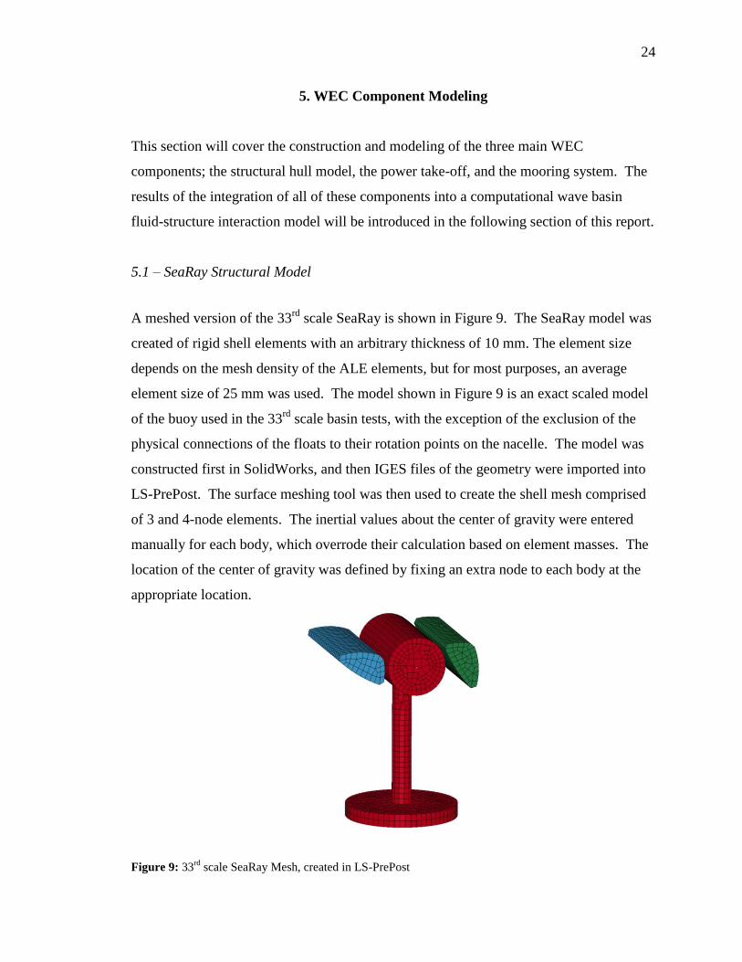
5.1 – SeaRay Structural Model
A meshed version of the 33rd
scale SeaRay is shown in Figure 9. The SeaRay model was
created of rigid shell elements with an arbitrary thickness of 10 mm. The element size
depends on the mesh density of the ALE elements, but for most purposes, an average
element size of 25 mm was used. The model shown in Figure 9 is an exact scaled model
of the buoy used in the 33rd
scale basin tests, with the exception of the exclusion of the
physical connections of the floats to their rotation points on the nacelle. The model was
constructed first in SolidWorks, and then IGES files of the geometry were imported into
LS-PrePost. The surface meshing tool was then used to create the shell mesh comprised
of 3 and 4-node elements. The inertial values about the center of gravity were entered
manually for each body, which overrode their calculation based on element masses. The
location of the center of gravity was defined by fixing an extra node to each body at the
appropriate location.
Figure 9: 33rd
scale SeaRay Mesh, created in LS-PrePost
25
During the testing of the geometry shown above in Figure 9, we observed two signs of
numerical instability. The first observation was that the motion of the water elements
located between the floats and the nacelle was very unnatural, and became increasingly
violent and unstable as the simulation continued. The second observation was the
continual decrease of the timestep from 4x10⁻⁴
at t=0, to about 1x10⁻⁶
by the end of the
simulation. Due to the ~ 20 mm gap between the forward and aft floats, coupling
pressures from the nacelle and floats were applied over only one element width. It was
observed that as the nacelle applied pressure to force out impinging water, the
compressive force immediately pushed the water element into the float. The resulting
coupling incompatibility between the nearby bodies results in numerical instability, and
subsequent crashing of the simulation. Another consequence of the small gap distance
was increased sloshing between the bodies. Since the timestep is controlled by the
smallest element in the domain, the computation became increasingly more costly as
fluid elements between the nacelle and floats became more dynamically active.
As a result, a new geometry was devised such that the small gap distance was eliminated,
but the hydrodynamics of the device would remain largely unchanged. The modified
SeaRay geometry is shown in Figure 10. The distance between the floats in the modified
geometry is too small to allow water to enter the gap, and the effectiveness of the filling
actions of the *IVF card are not affected. Since the fluid inside the bodies is air, forcing
instability due to coupling between the bodies is negligible since the air has zero density.
The part masses of the previous model were reduced to reflect the additional
displacement, and the inertial terms were kept the same in order to ensure the dynamics
were altered as little as possible.

26
Figure 10: Modified 33rd
scale SeaRay geometry
5.2 – Power Take-Off
Revolute joints were defined for the forward and aft floats by rigidly fixing extra nodes to
the three bodies at the point of rotation, located at the center of the nacelle. To simulate
PTO forces of the 33rd
scale model which were applied by rotary dashpots during tank
testing, linear rotational damping was defined for the joint rotation. If desired, LS-
DYNA has the capability to apply nonlinear damping as a function of the joint velocity.
The software can also simulate active control by defining damping as a function of other
available variables such as nodal displacements, velocities, accelerations, forces,
interpolating polynomials, intrinsic functions, and any combinations thereof [25]. This
functionality is quite remarkable, since it can be utilized in the future to model active
control systems such as latching control [32–34].
Stop angles/distances can be defined for any mechanical sliding connection such as a
revolute or sliding joint. In the event a WEC body exceeds a pre-defined maximum
rotation or displacement, a user-defined spring force can be applied to stop the movement
of the body. The end stop forces can be directly extracted from the result files, and can
be used as an additional verification tool for the end stop force transducers installed on
the 7th
scale SeaRay.
27
5.3 – Mooring
The three point mooring lines were modeled using non-linear discrete cable elements
with pretension. The lines were attached to the buoy reaction plate at even intervals of
120°. No viscous damping is applied to line motions, as this functionality is not available
with the current coupling algorithm. It is possible, however, to account for viscous
effects on the beam elements by defining intrinsic functions which apply external forcing
as a function of line velocity. The mooring lines were given a mass which equals the
mass of the water displaced minus the mass of the line to achieve the correct body force.
It is also possible to model chain, cable, floats, rope, and other mooring components
together for a complete dynamic analysis of mooring systems. Underwater floats which
are commonly used in three-point catenary mooring systems can be modeled as either a
point loading in the vertical direction, or as a volumetric void, which would give a more
accurate representation of the dynamic hydrostatic force. Failure criteria (in material data
form) can also be prescribed for various connections, which would be of great interest
when testing for extreme events such as 100-year waves or ship collisions.
If a higher level of detail is desired, strain rate dependent stiffness with separate curves
for loading and unloading can be defined. For even more precise studies, the capability
exists to model the mechanics of mooring component interaction with the seabed. For
instance, it is possible to model the force needed to pull a suction pile free from a muddy
bottom, although this application is above and beyond the scope of most hydrodynamic
studies.

28
6. Results
This section presents the results of initial efforts to model a wave energy converter using
the compressible fluid solver - Lagrangian solid solver coupling FSI capability in LS-
DYNA. Due to the complexity of modeling an entire WEC system, several studies
isolating different features were conducted to assess the modeling capability of the
software for various WEC components. The first subsection presents the test results
which quantify the speed increase and wave generation ability of the improved
computational wave basin. The second subsection presents a simplified analysis of the
7th
scale mooring system. The final two subsections present the results of FSI
simulations conducted with simple geometries, as well as with the complete integration
of the individual WEC components which were presented in Section 5.
6.1 – CWB Speed Tests
A series of tests were conducted to quantify the benefits of the improved CWB. The test
basins are constructed of 81,000 solid ALE water elements, with dimensions 4500 x 1500
x 1500. The wave input to the model is monochromatic with height 60 cm and a period
of 1.2 seconds. A cylindrical pile consisting of 50 mm shell elements was fixed in the
center of the basin, with 850 elements lying below the still water level. For the case of
the unimproved basin, a wavemaker consisting of 900 shell elements was positioned 100
mm from the inflow boundary. The addition of the wavemaker introduces an additional
900 fluid coupling points to the simulation. The coupling stiffness scale factor was 0.1.
The duration of gravity application was 1 second for the unimproved basin, and 0.075
seconds for the improved basin. All simulations were conducted on 4 nodes of 3 GHz
processors with 8 GB of RAM each.
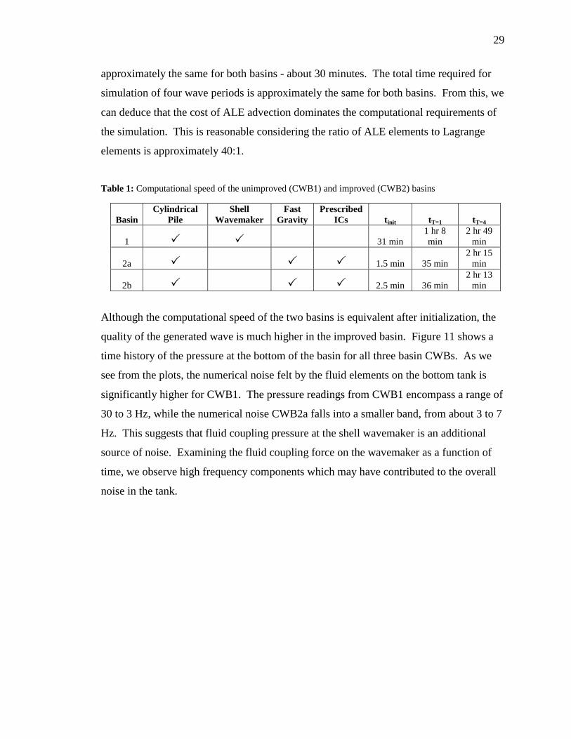
Table 1 shows the results of CWB speed testing. As we expect, the initialization time for
the unimproved basin (CWB1) is significantly larger than for the improved basin with
fast application of gravity and prescribed initial conditions (CWB2a, CWB2b).
Surprisingly though, after initialization, the time required to solve for one wave period is
29
approximately the same for both basins - about 30 minutes. The total time required for
simulation of four wave periods is approximately the same for both basins. From this, we
can deduce that the cost of ALE advection dominates the computational requirements of
the simulation. This is reasonable considering the ratio of ALE elements to Lagrange
elements is approximately 40:1.
Table 1: Computational speed of the unimproved (CWB1) and improved (CWB2) basins
Basin
Cylindrical
Pile
Shell
Wavemaker
Fast
Gravity
Prescribed
ICs tinit tT=1 tT=4
1 31 min
1 hr 8
min
2 hr 49
min
2a 1.5 min 35 min
2 hr 15
min
2b 2.5 min 36 min
2 hr 13
min
Although the computational speed of the two basins is equivalent after initialization, the
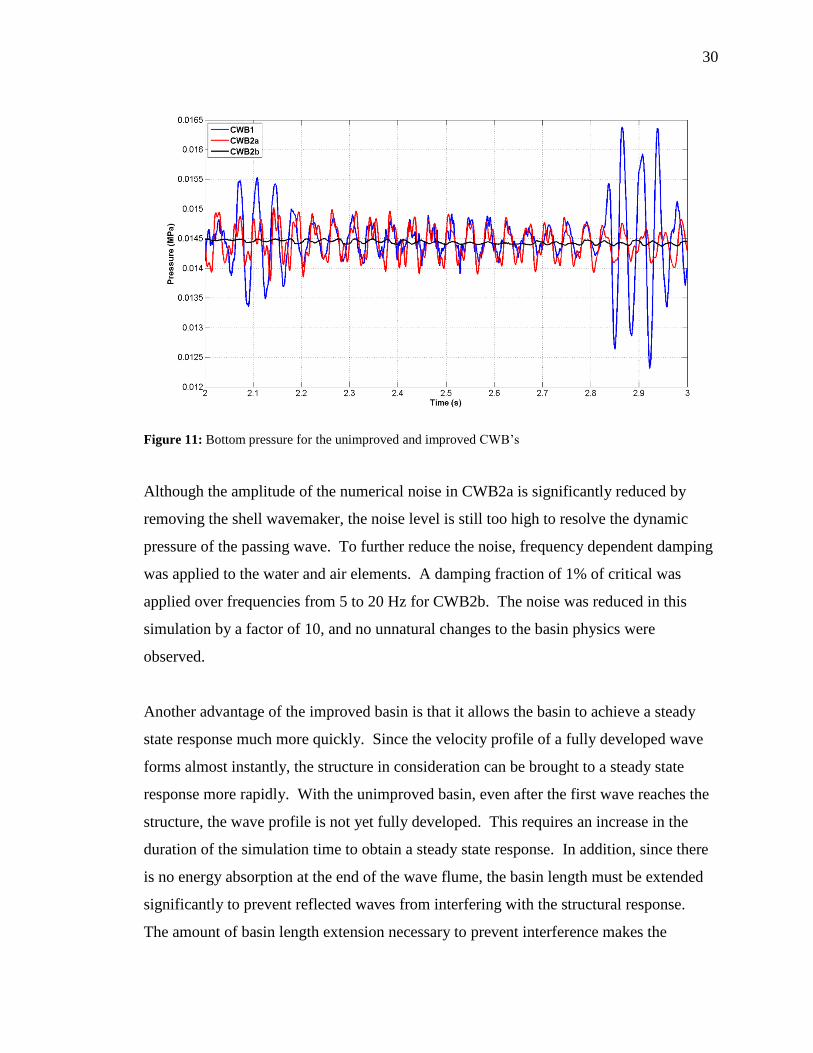
quality of the generated wave is much higher in the improved basin. Figure 11 shows a
time history of the pressure at the bottom of the basin for all three basin CWBs. As we
see from the plots, the numerical noise felt by the fluid elements on the bottom tank is
significantly higher for CWB1. The pressure readings from CWB1 encompass a range of
30 to 3 Hz, while the numerical noise CWB2a falls into a smaller band, from about 3 to 7
Hz. This suggests that fluid coupling pressure at the shell wavemaker is an additional
source of noise. Examining the fluid coupling force on the wavemaker as a function of
time, we observe high frequency components which may have contributed to the overall
noise in the tank.
30
Figure 11: Bottom pressure for the unimproved and improved CWB‟s
Although the amplitude of the numerical noise in CWB2a is significantly reduced by
removing the shell wavemaker, the noise level is still too high to resolve the dynamic
pressure of the passing wave. To further reduce the noise, frequency dependent damping
was applied to the water and air elements. A damping fraction of 1% of critical was
applied over frequencies from 5 to 20 Hz for CWB2b. The noise was reduced in this
simulation by a factor of 10, and no unnatural changes to the basin physics were
observed.
Another advantage of the improved basin is that it allows the basin to achieve a steady
state response much more quickly. Since the velocity profile of a fully developed wave
forms almost instantly, the structure in consideration can be brought to a steady state
response more rapidly. With the unimproved basin, even after the first wave reaches the
structure, the wave profile is not yet fully developed. This requires an increase in the
duration of the simulation time to obtain a steady state response. In addition, since there
is no energy absorption at the end of the wave flume, the basin length must be extended
significantly to prevent reflected waves from interfering with the structural response.
The amount of basin length extension necessary to prevent interference makes the
31
computational cost unacceptably high for this application, which highlights the need for
the improved CWB for these long-duration problems.
6.2 – Mooring Analysis
A common mooring system for WECs is a three-point catenary mooring system [35–37].
This system utilizes three main mooring legs spaced at even intervals in the radial
direction of the WEC. The system is designed such that the mooring tensions are low
when the WEC is operating about the center of the watch circle, but become increasingly
high when excursions become large. In this type of mooring design, the first leg of the
system extends away from the buoy, and connects to a submerged float which provides
additional stiffness to the system. The second leg connects the submerged float to the
anchor termination point.
To assess the capability of the nonlinear cable element in modeling WEC mooring
systems, two tests were devised. The first is a quasi-static model of the 7th
scale SeaRay
mooring system. Both legs of the mooring system were constructed using discrete cable
elements. A nonlinear stress-strain relationship was defined for the first leg of the system
which was comprised of ¾” nylon rope. The buoyant force of the submerged float was
defined as a nodal load in the global z-direction. The second leg of the system was ¾”
steel cable, which was defined to be linearly elastic. The mass of the materials was set to
be the difference between the mass of the displaced water and the wet line weight to
obtain the correct body force. To reduce oscillation in the lines from the initial
tensioning of the system, frequency dependent damping was applied from 0.5 to 20 Hz.
Pretension was held throughout the simulation, corresponding to the as-installed stiffness.
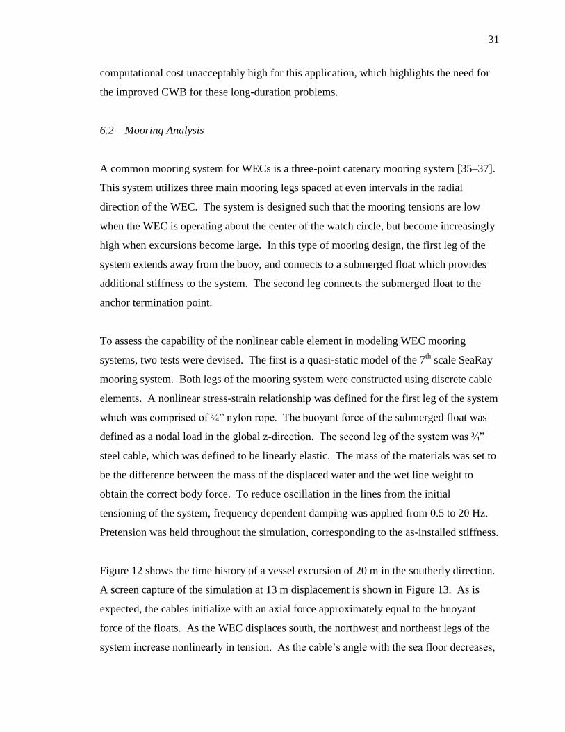
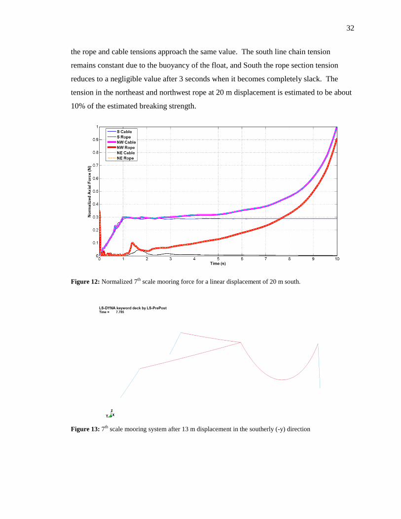
Figure 12 shows the time history of a vessel excursion of 20 m in the southerly direction.
A screen capture of the simulation at 13 m displacement is shown in Figure 13. As is
expected, the cables initialize with an axial force approximately equal to the buoyant
force of the floats. As the WEC displaces south, the northwest and northeast legs of the
system increase nonlinearly in tension. As the cable‟s angle with the sea floor decreases,
32
the rope and cable tensions approach the same value. The south line chain tension
remains constant due to the buoyancy of the float, and South the rope section tension
reduces to a negligible value after 3 seconds when it becomes completely slack. The
tension in the northeast and northwest rope at 20 m displacement is estimated to be about
10% of the estimated breaking strength.
Figure 12: Normalized 7th
scale mooring force for a linear displacement of 20 m south.
Figure 13: 7th
scale mooring system after 13 m displacement in the southerly (-y) direction
33
6.3 – Stability and Leakage Prevention for Simple Geometries
As an initial assessment of the leakage prevention and stability of the coupling algorithm,
several short numerical studies were conducted for simple geometric bodies in a
cylindrical basin. The first simulation was the case of a submerged 500 mm diameter
plate. Both ALE and Lagrangian elements had an average element size of 25 mm. The
plate was given an oscillatory z-velocity of 100 mm/s to test leakage prevention.
Iterating through several different stiffness cases, we observed that leakage could be
prevented using a stiffness factor and a leakage control factor of 0.1. For higher
stiffnesses, the internal air would push out of the structure and rise to the surface of the
basin. Lower stiffnesses resulted in gradual or immediate leakage.
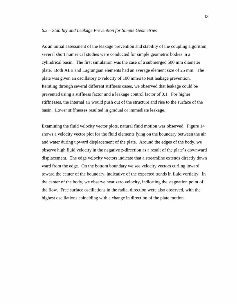
Examining the fluid velocity vector plots, natural fluid motion was observed. Figure 14
shows a velocity vector plot for the fluid elements lying on the boundary between the air
and water during upward displacement of the plate. Around the edges of the body, we
observe high fluid velocity in the negative z-direction as a result of the plate‟s downward
displacement. The edge velocity vectors indicate that a streamline extends directly down
ward from the edge. On the bottom boundary we see velocity vectors curling inward
toward the center of the boundary, indicative of the expected trends in fluid vorticity. In
the center of the body, we observe near zero velocity, indicating the stagnation point of
the flow. Free surface oscillations in the radial direction were also observed, with the
highest oscillations coinciding with a change in direction of the plate motion.

34
Figure 14: Fluid velocity vectors and streamlines for a submerged oscillating plate
For other similar, simplistic geometries constrained in heave or freely floating, numerical
stability was achieved indefinitely in a still numerical basin. Through the iterative testing
of several different geometries, it was observed that the stable coupling stiffness varies
significantly based on the mesh density (both fluid and structural domains), the fluid
properties such as speed of sound and viscosity, the number of ALE quadrature points,
and the maximum allowable fluid penetration. Although the coupling stiffness values
can be estimated based on the Courant number, this is only an approximation; the stable
stiffness values must be determined varied iteratively until stability is achieved. It was
also observed that numerical stability becomes more difficult to achieve as geometric
complexity increases, fluid flow becomes more violent, and the structure is given more
degrees of freedom.
6.4 – WEC Floatation and Stability in Still Water
Modeling the 33rd
scale SeaRay WEC presented many challenges due to its complex
geometry and multiple degrees of freedom. As mentioned previously, modifications to
the WEC geometry were made in order to reduce coupling incompatibility between the
floats and nacelle, and reduce the simulation time step. A screenshot of the modified
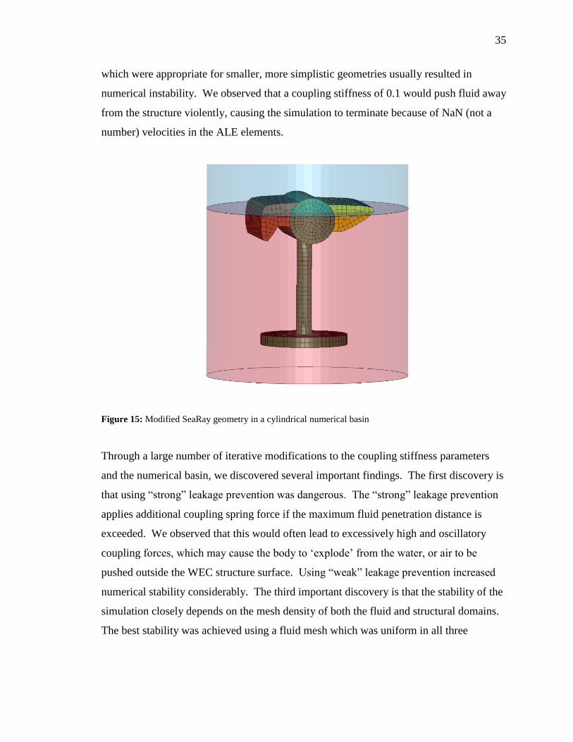
SeaRay geometry in a cylindrical numerical basin is shown in Figure 15. The first
observation of testing free floating WEC geometry was that the coupling parameters
35
which were appropriate for smaller, more simplistic geometries usually resulted in
numerical instability. We observed that a coupling stiffness of 0.1 would push fluid away
from the structure violently, causing the simulation to terminate because of NaN (not a
number) velocities in the ALE elements.
Figure 15: Modified SeaRay geometry in a cylindrical numerical basin
Through a large number of iterative modifications to the coupling stiffness parameters
and the numerical basin, we discovered several important findings. The first discovery is
that using “strong” leakage prevention was dangerous. The “strong” leakage prevention
applies additional coupling spring force if the maximum fluid penetration distance is
exceeded. We observed that this would often lead to excessively high and oscillatory
coupling forces, which may cause the body to „explode‟ from the water, or air to be
pushed outside the WEC structure surface. Using “weak” leakage prevention increased
numerical stability considerably. The third important discovery is that the stability of the
simulation closely depends on the mesh density of both the fluid and structural domains.
The best stability was achieved using a fluid mesh which was uniform in all three
36
dimensions, and had the same length dimension as the shell elements of the WEC
structure.
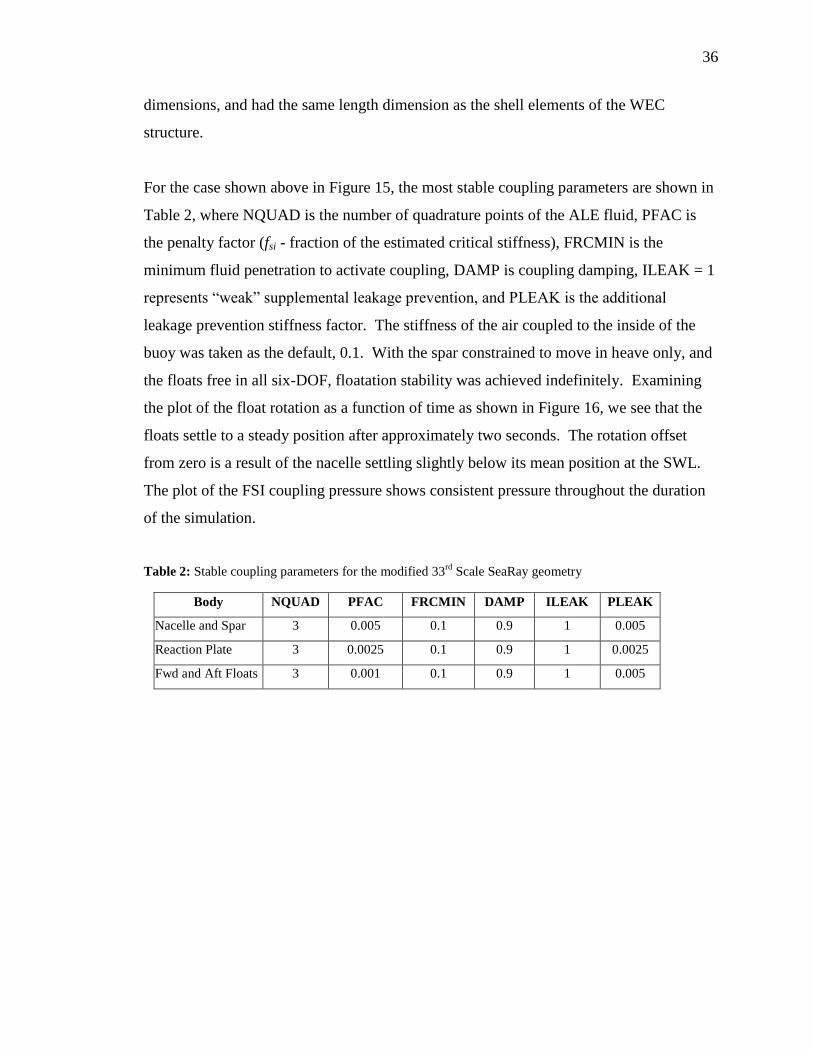
For the case shown above in Figure 15, the most stable coupling parameters are shown in
Table 2, where NQUAD is the number of quadrature points of the ALE fluid, PFAC is
the penalty factor (fsi - fraction of the estimated critical stiffness), FRCMIN is the
minimum fluid penetration to activate coupling, DAMP is coupling damping, ILEAK = 1
represents “weak” supplemental leakage prevention, and PLEAK is the additional
leakage prevention stiffness factor. The stiffness of the air coupled to the inside of the
buoy was taken as the default, 0.1. With the spar constrained to move in heave only, and
the floats free in all six-DOF, floatation stability was achieved indefinitely. Examining
the plot of the float rotation as a function of time as shown in Figure 16, we see that the
floats settle to a steady position after approximately two seconds. The rotation offset
from zero is a result of the nacelle settling slightly below its mean position at the SWL.
The plot of the FSI coupling pressure shows consistent pressure throughout the duration
of the simulation.
Table 2: Stable coupling parameters for the modified 33rd
Scale SeaRay geometry
Body NQUAD PFAC FRCMIN DAMP ILEAK PLEAK
Nacelle and Spar 3 0.005 0.1 0.9 1 0.005
Reaction Plate 3 0.0025 0.1 0.9 1 0.0025
Fwd and Aft Floats 3 0.001 0.1 0.9 1 0.005
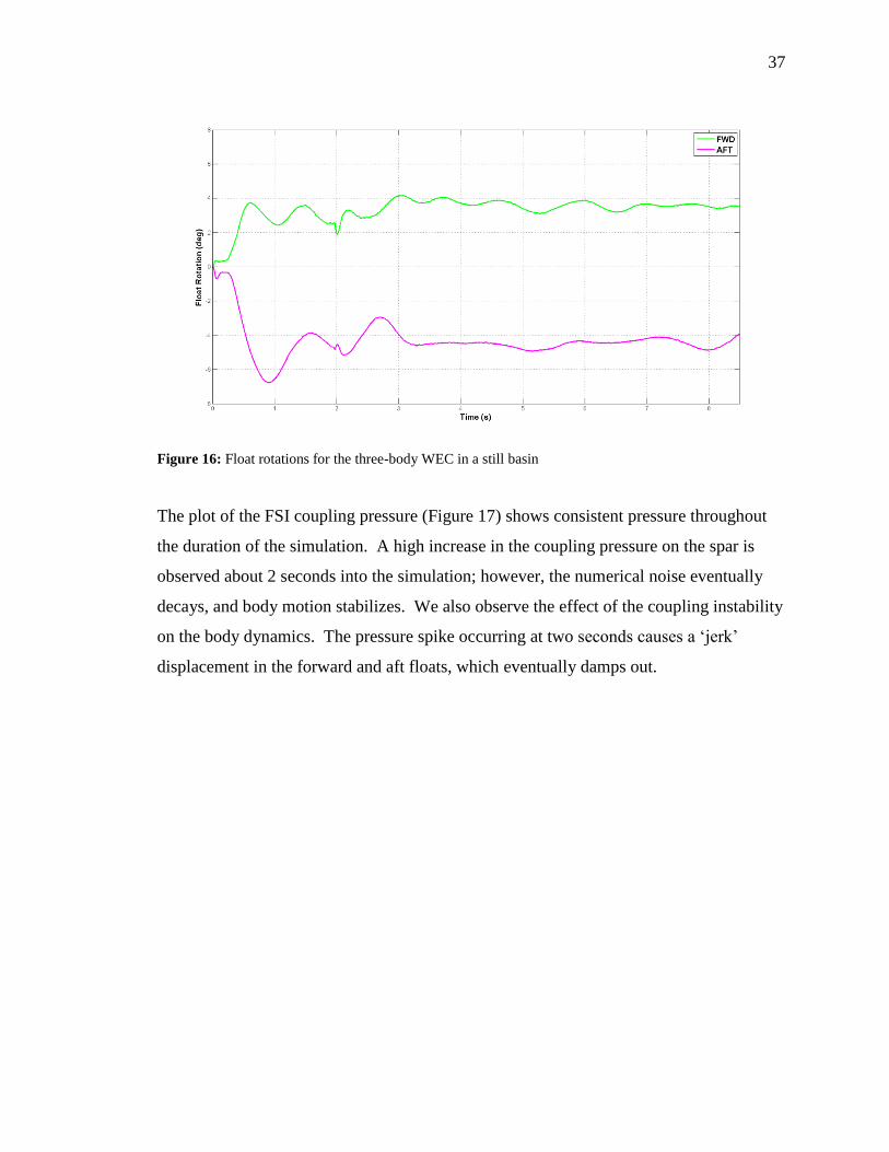
37
Figure 16: Float rotations for the three-body WEC in a still basin
The plot of the FSI coupling pressure (Figure 17) shows consistent pressure throughout
the duration of the simulation. A high increase in the coupling pressure on the spar is
observed about 2 seconds into the simulation; however, the numerical noise eventually
decays, and body motion stabilizes. We also observe the effect of the coupling instability
on the body dynamics. The pressure spike occurring at two seconds causes a „jerk‟
displacement in the forward and aft floats, which eventually damps out.
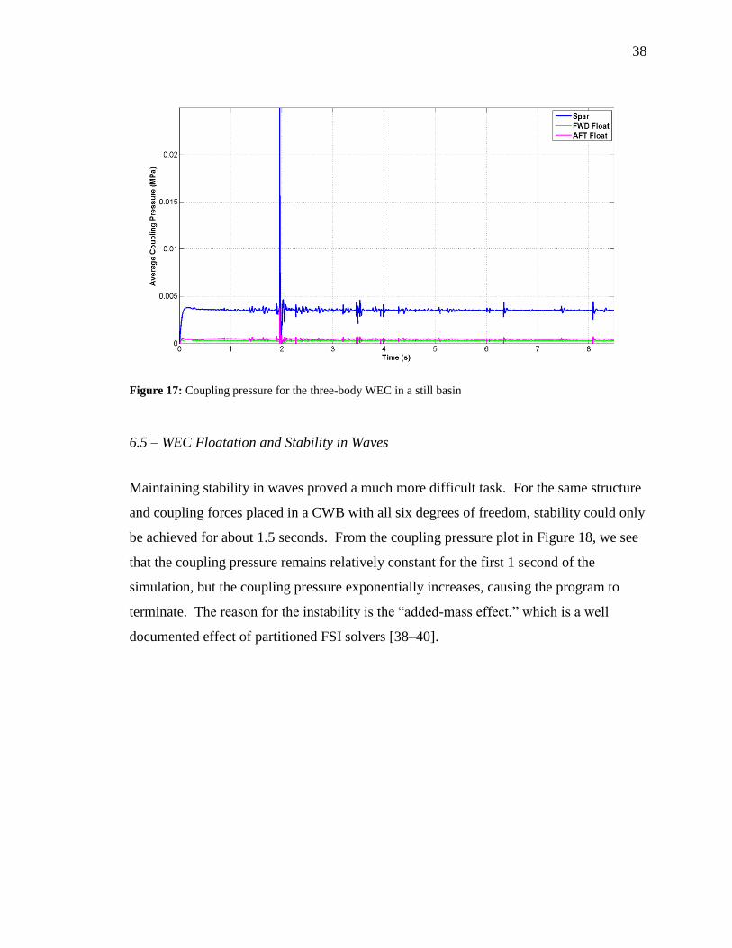
38
Figure 17: Coupling pressure for the three-body WEC in a still basin
6.5 – WEC Floatation and Stability in Waves
Maintaining stability in waves proved a much more difficult task. For the same structure
and coupling forces placed in a CWB with all six degrees of freedom, stability could only
be achieved for about 1.5 seconds. From the coupling pressure plot in Figure 18, we see
that the coupling pressure remains relatively constant for the first 1 second of the
simulation, but the coupling pressure exponentially increases, causing the program to
terminate. The reason for the instability is the “added-mass effect,” which is a well
documented effect of partitioned FSI solvers [38–40].
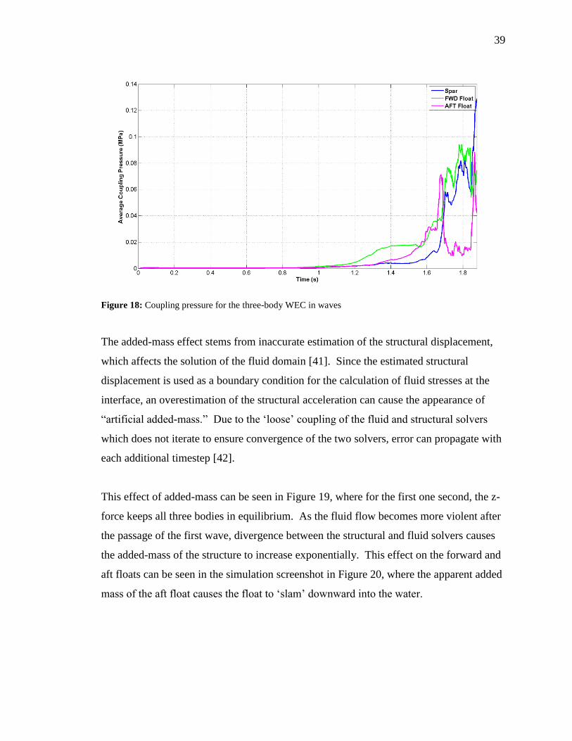
39
Figure 18: Coupling pressure for the three-body WEC in waves
The added-mass effect stems from inaccurate estimation of the structural displacement,
which affects the solution of the fluid domain [41]. Since the estimated structural
displacement is used as a boundary condition for the calculation of fluid stresses at the
interface, an overestimation of the structural acceleration can cause the appearance of
“artificial added-mass.” Due to the „loose‟ coupling of the fluid and structural solvers
which does not iterate to ensure convergence of the two solvers, error can propagate with
each additional timestep [42].
This effect of added-mass can be seen in Figure 19, where for the first one second, the z-
force keeps all three bodies in equilibrium. As the fluid flow becomes more violent after
the passage of the first wave, divergence between the structural and fluid solvers causes
the added-mass of the structure to increase exponentially. This effect on the forward and
aft floats can be seen in the simulation screenshot in Figure 20, where the apparent added
mass of the aft float causes the float to „slam‟ downward into the water.
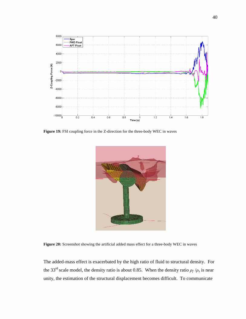
40
Figure 19: FSI coupling force in the Z-direction for the three-body WEC in waves
Figure 20: Screenshot showing the artificial added mass effect for a three-body WEC in waves
The added-mass effect is exacerbated by the high ratio of fluid to structural density. For
the 33rd
scale model, the density ratio is about 0.85. When the density ratio ρf /ρs is near
unity, the estimation of the structural displacement becomes difficult. To communicate

41
this point, an example is provided below which illustrates the „density ratio near unity‟
effect for a flexible cylindrical tube in constrained fluid flow [43].
(8)
where the term in the brackets is referred to as the „growth factor.‟ Assuming the
timestep is small, we can eliminate the first two terms of the expression, leading to
(9)
where µi is the ith
Eigenvalue of the added mass matrix, hs is the thickness of the flexible
cylinder, a is a temporal wave frequency, and k is a spatial wave frequency. We see from
this that the estimation of the structural displacement will become unstable for ρf /ρs ≥ 1.
We also observe that increasing the structural stiffness serves to increase the stability.
This may provide an explanation for the stability of simulations conducted in this study
with fixed or 1-DOF geometries.
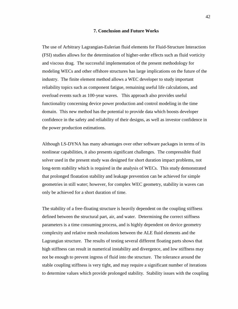
42
7. Conclusion and Future Works
The use of Arbitrary Lagrangian-Eulerian fluid elements for Fluid-Structure Interaction
(FSI) studies allows for the determination of higher-order effects such as fluid vorticity
and viscous drag. The successful implementation of the present methodology for
modeling WECs and other offshore structures has large implications on the future of the
industry. The finite element method allows a WEC developer to study important
reliability topics such as component fatigue, remaining useful life calculations, and
overload events such as 100-year waves. This approach also provides useful
functionality concerning device power production and control modeling in the time
domain. This new method has the potential to provide data which boosts developer
confidence in the safety and reliability of their designs, as well as investor confidence in
the power production estimations.
Although LS-DYNA has many advantages over other software packages in terms of its
nonlinear capabilities, it also presents significant challenges. The compressible fluid
solver used in the present study was designed for short duration impact problems, not
long-term stability which is required in the analysis of WECs. This study demonstrated
that prolonged floatation stability and leakage prevention can be achieved for simple
geometries in still water; however, for complex WEC geometry, stability in waves can
only be achieved for a short duration of time.
The stability of a free-floating structure is heavily dependent on the coupling stiffness
defined between the structural part, air, and water. Determining the correct stiffness
parameters is a time consuming process, and is highly dependent on device geometry
complexity and relative mesh resolutions between the ALE fluid elements and the
Lagrangian structure. The results of testing several different floating parts shows that
high stiffness can result in numerical instability and divergence, and low stiffness may
not be enough to prevent ingress of fluid into the structure. The tolerance around the
stable coupling stiffness is very tight, and may require a significant number of iterations
to determine values which provide prolonged stability. Stability issues with the coupling
43
algorithm are compounded by the compressibility of the fluid, which introduces high
frequency numerical noise into the numerical basin. Numerical noise can be reduced by
applying coupling stiffness damping, and frequency dependent damping to the fluid
elements; however, this does not alleviate all issues with the solver.
Despite stability issues associated with free-floating structures, this study has shown that
extensive capabilities exist within the software to model WEC components such as
mooring systems, power take-off and control, and structural elasticity. For simple
geometries, the simulation results yielded good stability, accurate body forces, and highly
nonlinear fluid particle velocities which show fluid vorticity and evidence of streamlines.
An improved computational wave basin capable of assessing structural response in
regular waves in a computationally efficient manner was created, which can be used in
future FSI studies on floating or fixed structures.
Evidence from this study shows that the current fluid solver is not suitable for long
duration FSI studies; we have observed that the structural solver is ready for even the
most demanding modeling challenges. The observed stability issues stemming from the
„loose coupling‟ of the current compressible ALE fluid and Lagrangian solid solvers has
highlighted the need for an implicit, incompressible fluid solver which can control the
timestep. An incompressible fluid solver is near the end of development which may
increase the applicability of LS-DYNA for hydrodynamic analysis of floating structures.
The incompressible solver will allow the fluid pressures to be calculated implicitly which
will provide two benefits: reduction in high frequency numerical noise, and
computational speed increase estimated at one to two orders of magnitude. It is expected
that the new fluid solver will alleviate numerical noise that is believed to be a large part
of the coupling instability and divergence of the loosely coupled FSI solvers. The
simulation speed increase will also allow the mesh density to be vastly increased without
excessive computational cost which should also increase stability.
Another functionality that must be developed for a fully coupled analysis is fluid
coupling between beam elements of the mooring lines and the fluid elements. This could

44
be accomplished using a slave/master search similar to the algorithm used for shell
coupling. Since the line diameter is much smaller than the water element size, and
surface-to-node coupling of the lines would be prohibitively computationally expensive,
a good approximation of the viscous effects on the line could be achieved using the
Morrison equation. This would extend LS-DYNA‟s capability to analyze the full
nonlinearity of mooring systems, and the fully-coupled structural response of a wave
energy converter.
The basis of knowledge generated by this research outlines the current capability of the
LS-DYNA for long-duration contact FSI problems involving floating structures.
Although the current research shows that hydrodynamic modeling of a wave energy
converter is still in need of improvement in order to be feasible at this time, we have
demonstrated that stability can be achieved for multiple-DOF systems in waves for
excess of 1 million timesteps. In the near future, we are optimistic that success in this
application can be achieved with the availability of the new incompressible fluid solver.
The modeling techniques and methodologies discovered by this research will serve as a
basis for future modeling efforts that seek to verify the accuracy of numerical results
using available data from Columbia Power Technologies 33rd
and 7th
scale tests.
45
Bibliography
[1] J. Cruz, Ocean Wave Energy: Current Status and Future Prespectives, 1st ed.,
Springer, 2008.
[2] N. Aquelet, ALE Modeling of Surface Waves, in: Gothenburg, Sweeden, 2005: pp.
4.9-4.20.
[3] C. Carmody, G. Burriesci, I. Howard, E.A. Patterson, The use of LS-DYNA fluid-
structure interaction to simulate fluid-driven deformation in the aortic valve, in:
Aerospace / Fluid-Structure Interaction, Ulm, Germany, 2003: pp. 11-20.
[4] M. Ghorbaine, G. Norlander, Structure-Fluid Interaction Analysis of and Existing
Water Tank, in: Fluids / FSI, Detroit, Michigan, 2010: pp. 6.5-6.18.
[5] K. Jackson, Y. Fuchs, Comparison of ALE and SPH Simulations of Vertical Drop
Tests of a Composite Fuselage Section into Water, in: Detroit, Michigan, 2008: pp.
1.1-1.20.
[6] M. Souli, Fluid-Structure Interaction in LS-DYNA: Industrial Applications, in:
Aerospace / Fluid-Structure Interaction, Ulm, Germany, 2003: pp. 35-42.
[7] M. Souli, J. Wang, I. Do, C. Hao, ALE and Fluid Structure Interaction in LS-
DYNA, in: Fluid/Structure, Detroit, Michigan, 2004: pp. 4.39-4.44.
[8] J. Wang, H. Chen, Fluid Structure Interaction for Immersed Bodies, in:
Gothenburg, Sweeden, 2005: pp. 4.3-4.8.
[9] M. Souli, A. Ouahsine, L. Lewin, ALE formulation for fluid-structure interaction
problems, Computer Methods in Applied Mechanics and Engineering. 190 (2000)
659-675.
[10] M. Souli, Eulerian and fluid-structure coupling algorithm in LS-DYNA, American
Society of Mechanical Engineers, Pressure Vessels and Piping Division
(Publication) PVP. 396 (1999) 269-274.
[11] I. Stenius, A. Rosén, J. Kuttenkeuler, Explicit FE-modelling of hydroelasticity in
panel-water impacts, International Shipbuilding Progress. 54 (2007) 111-127.
[12] W. Zhang, S. Yim, A Multiphysics Multiscale 3-D Computational Wave Basin
Model for Wave Impact Load on a Cylindrical Structure, Journal of Disaster
Research. 4 (2009) 450-461.
[13] S. Tokura, T. Ida, Simulation of Wave-Dissipating Mechanism on Submerged
Structure using Fluid-Structure Coupling Capability in LS-DYNA, in: 5th European
LS-DYNA Users Conference, Birmingham, England, 2005.
[14] I. Stenius, A. Rosen, J. Kuttenkeuler, Explicit FE-modelling of hydroelasticity in
panel-water impacts, International Shipbuilding Progress. 54 (2007) 111-127.
[15] M. Langeliers, E. Agamloh, A. Von Jouanne, A. Wallace, A permanent magnet,
rack and pinion gearbox for ocean energy extraction, in: 44th AIAA Aerospace
Sciences Meeting 2006, January 9, 2006 - January 12, 2006, Reno, NV, United
states, American Institute of Aeronautics and Astronautics Inc., 2006: pp. 11973-
11980.
[16] K. Rhinefrank, E.B. Agamloh, A. Von Jouanne, A.K. Wallace, J. Prudell, K.
Kimble, et al., Novel ocean energy permanent magnet linear generator buoy,
Renewable Energy. 31 (2006) 1279-1298.
46
[17] E.B. Agamloh, A.K. Wallace, A. von Jouanne, A novel direct-drive ocean wave
energy extraction concept with contact-less force transmission system, Renewable
Energy. 33 (2008) 520-529.
[18] D. Elwood, S.C. Yim, J. Prudell, C. Stillinger, A. von Jouanne, T. Brekken, et al.,
Design, construction, and ocean testing of a taut-moored dual-body wave energy
converter with a linear generator power take-off, Renewable Energy. 35 (2010)
348-354.
[19] D. Elwood, A. Schacher, K. Rhinefrank, J. Prudell, S. Yim, E. Amon, et al.,
Numerical modeling and ocean testing of a direct-drive wave energy device
utilizing a permanent magnet linear generator for power take-off, in: 28th
International Conference on Ocean, Offshore and Arctic Engineering, OMAE2009,
May 31, 2009 - June 5, 2009, Honolulu, HI, United states, American Society of
Mechanical Engineers, 2009: pp. 817-824.
[20] K. Rhinefrank, A. Schacher, J. Prudell, E. Hammagren, C. Stillinger, D. Naviaux,
et al., Scaled wave energy device performance evaluation through high resolution
wave tank testing, in: MTS/IEEE Seattle, OCEANS 2010, September 20, 2010 -
September 23, 2010, Seattle, WA, United states, IEEE Computer Society, 2010.
[21] K. Rhinefrank, A. Schacher, J. Prudell, J. Cruz, N. Jorge, C. Stillinger, et al.,
Numerical and Experimental Analysis of a Novel Wave Energy Converter, ASME
Conf. Proc. 2010 (2010) 559-567.
[22] M. Haller, A. Porter, P. Lenee-Bluhm, K. Rhinefrank, E. Hammagren, T. Ozkan-
Haller, et al., Laboratory Observations of Waves in the Vicinity of WEC-Arrays, in:
Southampton, England, 2011.
[23] B. van Leer, Towards the ultimate conservative difference scheme. V. A second-
order sequel to Godunov‟s method, Journal of Computational Physics. 32 (1979)
101-136.
[24] D.J. Benson, Momentum advection on a staggered mesh, Journal of Computational
Physics. 100 (1992) 143-162.
[25] J. Halquist, LS-DYNA Theory Manual, (2006).
[26] M. Souli, D.J. Benson, Arbitrary Lagrangian Eulerian and Fluid-Structure
Interaction: Numerical Simulation, 1st ed., Wiley-ISTE, 2010.
[27] I. Stenius, A. Rosén, J. Kuttenkeuler, Explicit FE-modelling of fluid-structure
interaction in hull-water impacts, International Shipbuilding Progress. 53 (2006)
103-121.
[28] C. Forster, W. Wall, E. Ramm, The artificial Added Mass Effect in Sequential
Staggered Fluid-Structure Interaction Algorithms, in: Delft, The Netherlands, 2006:
pp. 1-20.
[29] S. Tokura, T. Ida, Simulation of Wave-Dissipating Mechanism on Submerged
Structure Using Fluid-Structure Coupling Capability in LS-DYNA, in: ALE, FSI,
SPH (1), Birmingham, England, n.d.
[30] N. Aquelet, C. Seddon, M. Souli, M. Moatamedi, Initialisation of volume fraction
in fluid/structure interaction problem, International Journal of Crashworthiness. 10
(2005) 237-247.
[31] R.G. Dean, R.A. Dalrymple, Water Wave Mechanics for Engineers & Scientists
(Advanced Series on Ocean Engineering-Vol2), World Scientific Pub Co Inc, 1991.

47
[32] J. Hals, T. Bjarte-Larsson, J. Falnes, Optimum reactive control and control by
latching of a wave-absorbing semisubmerged heaving sphere, in: Proceedings of the
21st International Conference on Offshore Mechanics and Arctic Engineering
(OMAE), June 23, 2002 - June 28, 2002, Oslo, Norway, American Society of
Mechanical Engineers, 2002: pp. 415-423.
[33] T. Bjarte-Larsson, J. Falnes, Laboratory experiment on heaving body with
hydraulic power take-off and latching control, Ocean Engineering. 33 (2006) 847-
877.
[34] J. Falnes, T. Bjarte-Larsson, Theoretical and experimental investigation of wave
energy conversion by a phase-controlled heaving body, Proceedings of the
Institution of Mechanical Engineers Part M: Journal of Engineering for the
Maritime Environment. 220 (2006) 175-183.
[35] Reedsport OPT Wave Park Settlement Agreement, (2010).
[36] J. Fitzgerald, L. Bergdahl, Including moorings in the assessment of a generic
offshore wave energy converter: A frequency domain approach, Marine Structures.
21 (2008) 23-46.
[37] P.C. Vicente, A.F. de O. Falcão, L.M.C. Gato, P.A.P. Justino, Dynamics of arrays
of floating point-absorber wave energy converters with inter-body and bottom
slack-mooring connections, Applied Ocean Research. 31 (2009) 267-281.
[38] P. Causin, J.F. Gerbeau, F. Nobile, Added-mass effect in the design of partitioned
algorithms for fluid-structure problems, Computer Methods in Applied Mechanics
and Engineering. 194 (2005) 4506-4527.
[39] S.R. Idelsohn, F. Del Pin, R. Rossi, E. Onate, Fluid-structure interaction problems
with strong added-mass effect, International Journal for Numerical Methods in
Engineering. 80 (2009) 1261-1294.
[40] C. Forster, W.A. Wall, E. Ramm, Artificial added mass instabilities in sequential
staggered coupling of nonlinear structures and incompressible viscous flows,
Computer Methods in Applied Mechanics and Engineering. 196 (2007) 1278-1293.
[41] S.R. Idelsohn, F. Del Pin, R. Rossi, E. Onate, Fluid-structure interactions problems
including added-mass effect, in: Venice, Italy, 2008.
[42] J.R. Cebral, R. Lohner, On the loose coupling of implicit time-marching codes, in:
43rd AIAA Aerospace Sciences Meeting and Exhibit, January 10, 2005 - January
13, 2005, Reno, NV, United states, American Institute of Aeronautics and
Astronautics Inc., 2005: pp. 10079-10093.
[43] P. Thavornpattanapong, K. Wong, S. Cheung, J. Tu, Mathematical Analysis of
Added-Mass Instability in Fluid-Structure Interaction, International Journal of
Mathematics and Statistics. 10 (2011).
[44] J. Day, Guidelines for ALE Modeling in LS-DYNA, Internal Document. Draft
2009 (2009).

48
APPENDICES
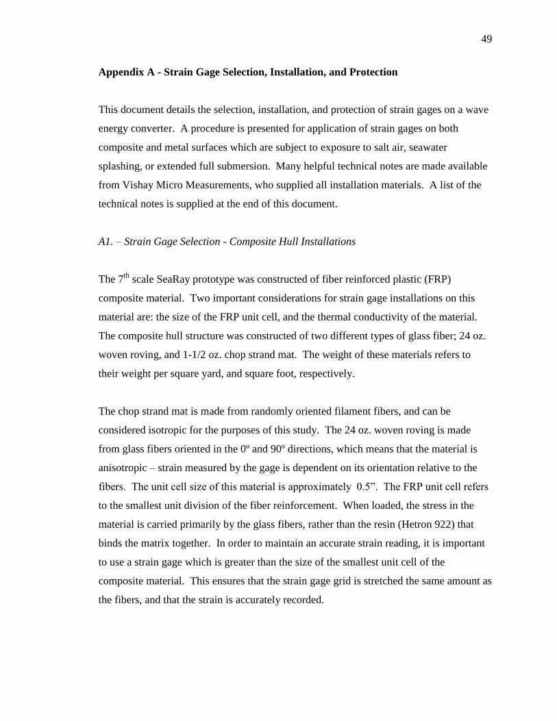
49
Appendix A - Strain Gage Selection, Installation, and Protection
This document details the selection, installation, and protection of strain gages on a wave
energy converter. A procedure is presented for application of strain gages on both
composite and metal surfaces which are subject to exposure to salt air, seawater
splashing, or extended full submersion. Many helpful technical notes are made available
from Vishay Micro Measurements, who supplied all installation materials. A list of the
technical notes is supplied at the end of this document.
A1. – Strain Gage Selection - Composite Hull Installations
The 7th
scale SeaRay prototype was constructed of fiber reinforced plastic (FRP)
composite material. Two important considerations for strain gage installations on this
material are: the size of the FRP unit cell, and the thermal conductivity of the material.
The composite hull structure was constructed of two different types of glass fiber; 24 oz.
woven roving, and 1-1/2 oz. chop strand mat. The weight of these materials refers to
their weight per square yard, and square foot, respectively.
The chop strand mat is made from randomly oriented filament fibers, and can be
considered isotropic for the purposes of this study. The 24 oz. woven roving is made
from glass fibers oriented in the 0º and 90º directions, which means that the material is
anisotropic – strain measured by the gage is dependent on its orientation relative to the
fibers. The unit cell size of this material is approximately 0.5”. The FRP unit cell refers
to the smallest unit division of the fiber reinforcement. When loaded, the stress in the
material is carried primarily by the glass fibers, rather than the resin (Hetron 922) that
binds the matrix together. In order to maintain an accurate strain reading, it is important
to use a strain gage which is greater than the size of the smallest unit cell of the
composite material. This ensures that the strain gage grid is stretched the same amount as
the fibers, and that the strain is accurately recorded.
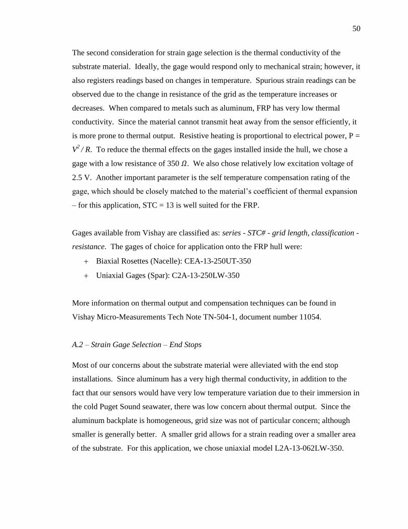
50
The second consideration for strain gage selection is the thermal conductivity of the
substrate material. Ideally, the gage would respond only to mechanical strain; however, it
also registers readings based on changes in temperature. Spurious strain readings can be
observed due to the change in resistance of the grid as the temperature increases or
decreases. When compared to metals such as aluminum, FRP has very low thermal
conductivity. Since the material cannot transmit heat away from the sensor efficiently, it
is more prone to thermal output. Resistive heating is proportional to electrical power, P =
V2
/ R. To reduce the thermal effects on the gages installed inside the hull, we chose a
gage with a low resistance of 350 . We also chose relatively low excitation voltage of
2.5 V. Another important parameter is the self temperature compensation rating of the
gage, which should be closely matched to the material‟s coefficient of thermal expansion
– for this application, STC = 13 is well suited for the FRP.
Gages available from Vishay are classified as: series - STC# - grid length, classification -
resistance. The gages of choice for application onto the FRP hull were:
Biaxial Rosettes (Nacelle): CEA-13-250UT-350
Uniaxial Gages (Spar): C2A-13-250LW-350
More information on thermal output and compensation techniques can be found in
Vishay Micro-Measurements Tech Note TN-504-1, document number 11054.
A.2 – Strain Gage Selection – End Stops
Most of our concerns about the substrate material were alleviated with the end stop
installations. Since aluminum has a very high thermal conductivity, in addition to the
fact that our sensors would have very low temperature variation due to their immersion in
the cold Puget Sound seawater, there was low concern about thermal output. Since the
aluminum backplate is homogeneous, grid size was not of particular concern; although
smaller is generally better. A smaller grid allows for a strain reading over a smaller area
of the substrate. For this application, we chose uniaxial model L2A-13-062LW-350.

51
A.3 – Strain Gage Installation
Correct installation of strain gages is very important and time consuming task. Taking
your time during installation will dramatically reduce the amount of failures. It is
advisable to practice several times with old gages on scrap substrate before attempting an
installation. The installation procedure the hull gages installed on FRP and the end stop
gages installed on aluminum were more or less the same. A great wealth of information
and procedures on the installation and installation verification of strain gages on Vishay
Micro-Measurements website. The reader should consult the documents listed below for
detailed instruction.
1. Cleaning and surface conditioning of the substrate, installation of the gage:
Instruction Bulletin B-137 (Strain Gage Applications with M-Bond AE-10)
2. Surface conditioning for FRP gages: Application Note VMM-19 (Surface
preparation for composites)
A.4 – Strain Gage Protection
Without additional protection, strain gages installed in an ocean environment can be
expected to fail within days, if not hours of installation, even if they are not in direct
contact with seawater. Corrosion from can cause resistance increase in the circuitry,
seawater can cause short circuits, gages can be ripped from their substrate by waves – the
possibilities for failure are daunting, but there are several precautions we can take to
protect our installations.
The following procedure is used for the protection of any gages which have any
possibility of direct contact with seawater during the deployment. Figure 21 shows the
sequence of protective layers applied over the strain gage, terminal strips and leadwires.
Each coating should extend past the edges of the previous layer. It is important to note
that you must condition the surface of the substrate over the ENTIRE area which will be
covered by protective coatings. For this reason, it is recommended to scrub the surface

52
(but not sand!) with surface with the conditioners between each application step. Be sure
to wear gloves and an approved respirator, and work in a well ventilated area when using
these materials – they‟re toxic!
Figure 21: Protective layers applied over a strain gage subject to immersion in seawater
Application of the coatings is as follows:
1. Allow the gage adhesive to cure entirely before application of subsequent layers.
M-Bond AE-10 can be used within 6 hours, but the cure will achieve maximum
hardness and elongation capability after 24 to 48 hours.
2. Solder the leadwires to the gage and the terminal strip. Remove the solder flux.
Apply a thin coating of M-Coat A epoxy onto the gage surface, the solder points,
visible leadwires, and the terminal strip. Apply a thin layer, but allow a small
amount of the coating to extend over the sides of the gage and terminal strip.
Allow the coating to cure entirely.
3. Coat the leadwire outer casing with a thin layer of M-Coat B. This layer performs
three functions; it plugs any pinholes in the wire casing, acts as another water
barrier protecting the wire, and helps the next layers to better adhere to the wire.
Be sure to get a good amount of material buildup around the casing entrance and
the lead insulation. This will prevent water from entering or exiting the gage area
via the leadwire casing. After the wires have cured, try not to touch them, as oils
from your hands will affect the bonds.
4. Coat the entire gage area with a coating of M-Coat J, about 0.25” thick. This
coating should extend over the leadwire casing.
Specimen Terminal Strip
M-Coat B Leadwires Gagekote #5
Aluminum Foil
Strain Gage
M-Coat A

53
5. Cut a piece of aluminum which is big enough to extend over the first M-Coat J
coating. The aluminum acts as a vapor barrier. Any water vapor entering into the
gage area will have to go around the aluminum. For this reason, the aluminum
sheet should extend past the edges of the previous coat by about 1/8”. To apply
this coating, slather a thin layer of M-Coat J on the back of the Al sheet, and then
press it onto the previously cured layer. Some material should squeeze out from
all sides.
6. Apply another 0.25” layer of M-Coat J on top of the Aluminum sheet. If possible,
extend the coating as far up the leadwire casing as is reasonable.
Although the amount of material added on top of each gage seems extreme, these
coatings really do the trick. All installations conducted with this methodology have
survived three months (to date) on the SeaRay 7th
scale WEC, which was deployed in the
Puget Sound in February 2011.
Additional References:
Protection: Document Number 11025 (Protective Coatings)
Materials: Instruction Bulletin 176 (Installation of GageKote #5)
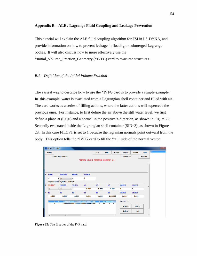
54
Appendix B – ALE / Lagrange Fluid Coupling and Leakage Prevention
This tutorial will explain the ALE fluid coupling algorithm for FSI in LS-DYNA, and
provide information on how to prevent leakage in floating or submerged Lagrange
bodies. It will also discuss how to more effectively use the
*Initial_Volume_Fraction_Geometry (*IVFG) card to evacuate structures.
B.1 – Definition of the Initial Volume Fraction
The easiest way to describe how to use the *IVFG card is to provide a simple example.
In this example, water is evacuated from a Lagrangian shell container and filled with air.
The card works as a series of filling actions, where the latter actions will supercede the
previous ones. For instance, to first define the air above the still water level, we first
define a plane at (0,0,0) and a normal in the positive z-direction, as shown in Figure 22.
Secondly evacuated inside the Lagrangian shell container (SID=3), as shown in Figure
23. In this case FILOPT is set to 1 because the lagranian normals point outward from the
body. This option tells the *IVFG card to fill the “tail” side of the normal vector.
Figure 22: The first tier of the IVF card
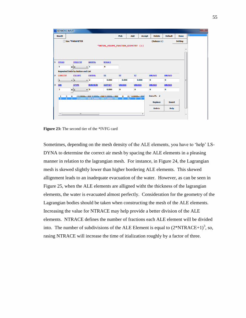
55
Figure 23: The second tier of the *IVFG card
Sometimes, depending on the mesh density of the ALE elements, you have to „help‟ LS-
DYNA to determine the correct air mesh by spacing the ALE elements in a pleasing
manner in relation to the lagrangian mesh. For instance, in Figure 24, the Lagrangian
mesh is skewed slightly lower than higher bordering ALE elements. This skewed
allignment leads to an inadequate evacuation of the water. However, as can be seen in
Figure 25, when the ALE elements are alligned witht the thickness of the lagrangian
elements, the water is evacuated almost perfectly. Consideration for the geometry of the
Lagrangian bodies should be taken when constructing the mesh of the ALE elements.
Increasing the value for NTRACE may help provide a better division of the ALE
elements. NTRACE defines the number of fractions each ALE element will be divided
into. The number of subdivisions of the ALE Element is equal to (2*NTRACE+1)3, so,
rasing NTRACE will increase the time of itialization roughly by a factor of three.
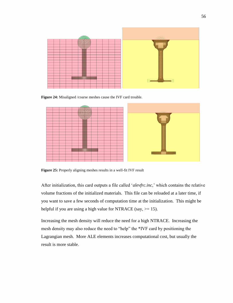
56
Figure 24: Misaligned /coarse meshes cause the IVF card trouble.
Figure 25: Properly aligning meshes results in a well-fit IVF result
After initialization, this card outputs a file called „alevfrc.inc,‟ which contains the relative
volume fractions of the initialized materials. This file can be reloaded at a later time, if
you want to save a few seconds of computation time at the initialization. This might be
helpful if you are using a high value for NTRACE (say, >= 15).
Increasing the mesh density will reduce the need for a high NTRACE. Increasing the
mesh density may also reduce the need to “help” the *IVF card by positioning the
Lagrangian mesh. More ALE elements increases computational cost, but usually the
result is more stable.
57
B.2 –Constrained Lagrange in Solid
This card is used to define contact between the ALE elements of the water and air and the
Lagrangian surface. Fluid coupling is by far and wide the most difficult aspect of ALE
modeling in LS-DYNA. Before attempting to use this card to prevent leakage in a
floating structure, it is highly recommended that you thoroughly read these documents:
LS-DYNA Keyword Manual - *Constrained_Lagrange_in_solid
[44] Day (2009 Internal LSTC Draft) - Guidelines for ALE Modeling in LS-
DYNA
[25] LS-DYNA Theory Manual - 26. Contact-Impact Algorithm (Penalty Method)
[27] Stenius, Rosén, Kuttenkeuler (2006) - Explicit FE-modelling of fluid-
structure interaction in hull-water impacts
This tutorial will assume that the above documents have been read thoroughly, and that
the user has a decent understanding of the contact/impact algorithms used in LS-DYNA.
Therefore, the rest of this document will describe proper modeling processes, and show a
few modeling tricks.
B.3 – The *Constrained_Lagrange_in_Solid Card
The contact that is defined by the *Constrained_Lagrange_in_Solid (*CLiS) card uses
either the Standard Penalty Method (ALE nodes coupled to Lagrange segments), or the
Segment-based Penalty Method (ALE Segments to Lagrange Segments). The penalty
method applies a spring force onto the ALE elements to push the liquid back out of the
structure, depending on the amount of element leakage into the structure. Determination
of the correct contact stiffness is by far the most difficult and frustrating aspect of this
type of modeling. Since the compressible coupling algorithm is not designed for
prolonged durations (>2 seconds), the choice of the stiffness constants needs to be
delicate if any numerical stability is to be achieved.
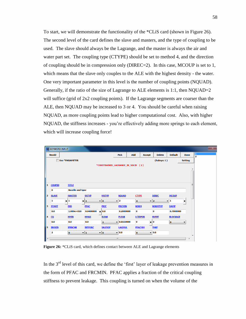
58
To start, we will demonstrate the functionality of the *CLiS card (shown in Figure 26).
The second level of the card defines the slave and masters, and the type of coupling to be
used. The slave should always be the Lagrange, and the master is always the air and
water part set. The coupling type (CTYPE) should be set to method 4, and the direction
of coupling should be in compression only (DIREC=2). In this case, MCOUP is set to 1,
which means that the slave only couples to the ALE with the highest density - the water.
One very important parameter in this level is the number of coupling points (NQUAD).
Generally, if the ratio of the size of Lagrange to ALE elements is 1:1, then NQUAD=2
will suffice (grid of 2x2 coupling points). If the Lagrange segments are coarser than the
ALE, then NQUAD may be increased to 3 or 4. You should be careful when raising
NQUAD, as more coupling points lead to higher computational cost. Also, with higher
NQUAD, the stiffness increases - you‟re effectively adding more springs to each element,
which will increase coupling force!
Figure 26: *CLiS card, which defines contact between ALE and Lagrange elements
In the 3rd
level of this card, we define the „first‟ layer of leakage prevention measures in
the form of PFAC and FRCMIN. PFAC applies a fraction of the critical coupling
stiffness to prevent leakage. This coupling is turned on when the volume of the

59
penetrating ALE element is greater than FRCMIN. The coupling stiffness can be thought
of as a spring-mass-damper system. If you think the spring force is being applied too
hastily, you can apply damping (velocity proportional). Information on how the critical
stiffness is estimated can be found in the LS-DYNA Theory Manual, page 26.9.
According to the keyword manual, you can define a load curve for the coupling stiffness
of PFAC, but currently, evidence shows that this functionality does not work correctly.
In the 4th
layer of this card, we define the „second‟ layer of leakage prevention. ILEAK
can be turned to 1 for “weak” protection (on when penetration >FRCMIN+0.1), or 2 for
“strong” protection (on when penetration > FRCMIN+0.3). ILEAK provides additional
coupling stiffness in addition to the 3rd
level when the penetrating fraction is too high.
PLEAK defines the additional coupling stiffness, and is conceptually similar to PFAC.
One of the most important things to remember is that the best stiffness is one that
provides just enough force to prevent leakage, and not more. If the stiffness is too high,
you run the risk of artificially injecting energy into the system by forcing the water away
with an unnecessary amount of force. This will effectively amount to additional
radiation. If the stiffness is much too high, sometimes you will observe the structure
„exploding‟ out of the basin.
B.4 – Fluid Coupling
The conditions of the coupling are as important for the water as they are for air. In order
to achieve maximum coupling stability, you must define a series of cards for each body
which define the coupling fluids, and their coupling direction with respect to the
Lagrangian surface. At this point, it seems that the best practice is to couple each
separate body with three separate ALE parts – the water and air filling the computational
domain, and a separate air part for the air inside the hollow shell body. Properly defining
these separate parts and their respective couplings for each body is complicated, so we
will provide an example below.

60
For the case of the three-body WEC shown in Figure 27, we see that there are separate
parts for the air and water in the computational domain (shown as the brown and red wire
around the edges), as well as for the air inside the bodies in yellow, blue and green. As
can be seen from the figure, the air domains are well fit inside the shell elements. The
body air parts are created using the *Initial_volume_fraction (*IVF) card, which creates
separate ALE parts, depending on the filling sequence.
Figure 27: WEC geometry with separate ALE domains for the air inside the bodies.
First, you must define “empty” parts which trick the *IVF card into thinking there is a
pre-defined mesh for the air parts. For this example, parts 7-9 were created with solid
ALE section and vacuum material for the separate air parts. No mesh is defined for these
parts. After the “empty” parts are created, define them as ALE elements in *ALE_Multi-
Material_Group (ALEMMG). So far, the ALEMMG card has the following groups: 1.
Water (domain), 2. Air (domain), 3. Air inside nacelle, 4. Air inside FWD float, 5. Air
inside AFT float.
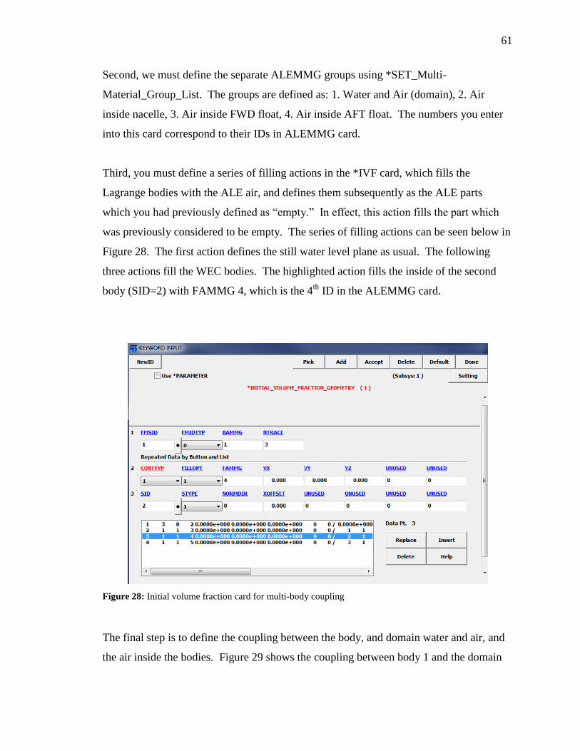
61
Second, we must define the separate ALEMMG groups using *SET_Multi-
Material_Group_List. The groups are defined as: 1. Water and Air (domain), 2. Air
inside nacelle, 3. Air inside FWD float, 4. Air inside AFT float. The numbers you enter
into this card correspond to their IDs in ALEMMG card.
Third, you must define a series of filling actions in the *IVF card, which fills the
Lagrange bodies with the ALE air, and defines them subsequently as the ALE parts
which you had previously defined as “empty.” In effect, this action fills the part which
was previously considered to be empty. The series of filling actions can be seen below in
Figure 28. The first action defines the still water level plane as usual. The following
three actions fill the WEC bodies. The highlighted action fills the inside of the second
body (SID=2) with FAMMG 4, which is the 4th
ID in the ALEMMG card.
Figure 28: Initial volume fraction card for multi-body coupling
The final step is to define the coupling between the body, and domain water and air, and
the air inside the bodies. Figure 29 shows the coupling between body 1 and the domain

62
water and air. The body is coupled to the domain water and air only by defining MCOUP
= -1, which links to ID 1 from the *Set_Multi-Material_Group_List. The direction is
compression only (DIREC=2), since we only want to prevent the water from moving into
the shell. Compressive direction refers to the force applied by the Lagrangian segment
on the water e.g. the segment force acts outward, compressing the ALE element.
Figure 29: Fluid coupling of the body to the domain water and air
Another coupling definition is needed for body 1 to couple with the air inside. A second
coupling is defined as shown in Figure 30, with MCOUP = -2 (couple with air inside the
nacelle only), and NORM = 1 (reverses the shell normal for compressive coupling inside
the shell).
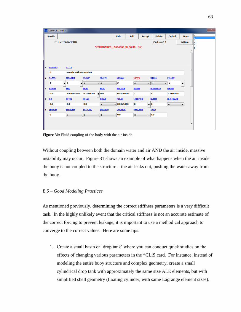
63
Figure 30: Fluid coupling of the body with the air inside.
Without coupling between both the domain water and air AND the air inside, massive
instability may occur. Figure 31 shows an example of what happens when the air inside
the buoy is not coupled to the structure – the air leaks out, pushing the water away from
the buoy.
B.5 – Good Modeling Practices
As mentioned previously, determining the correct stiffness parameters is a very difficult
task. In the highly unlikely event that the critical stiffness is not an accurate estimate of
the correct forcing to prevent leakage, it is important to use a methodical approach to
converge to the correct values. Here are some tips:
1. Create a small basin or „drop tank‟ where you can conduct quick studies on the
effects of changing various parameters in the *CLiS card. For instance, instead of
modeling the entire buoy structure and complex geometry, create a small
cylindrical drop tank with approximately the same size ALE elements, but with
simplified shell geometry (floating cylinder, with same Lagrange element sizes).
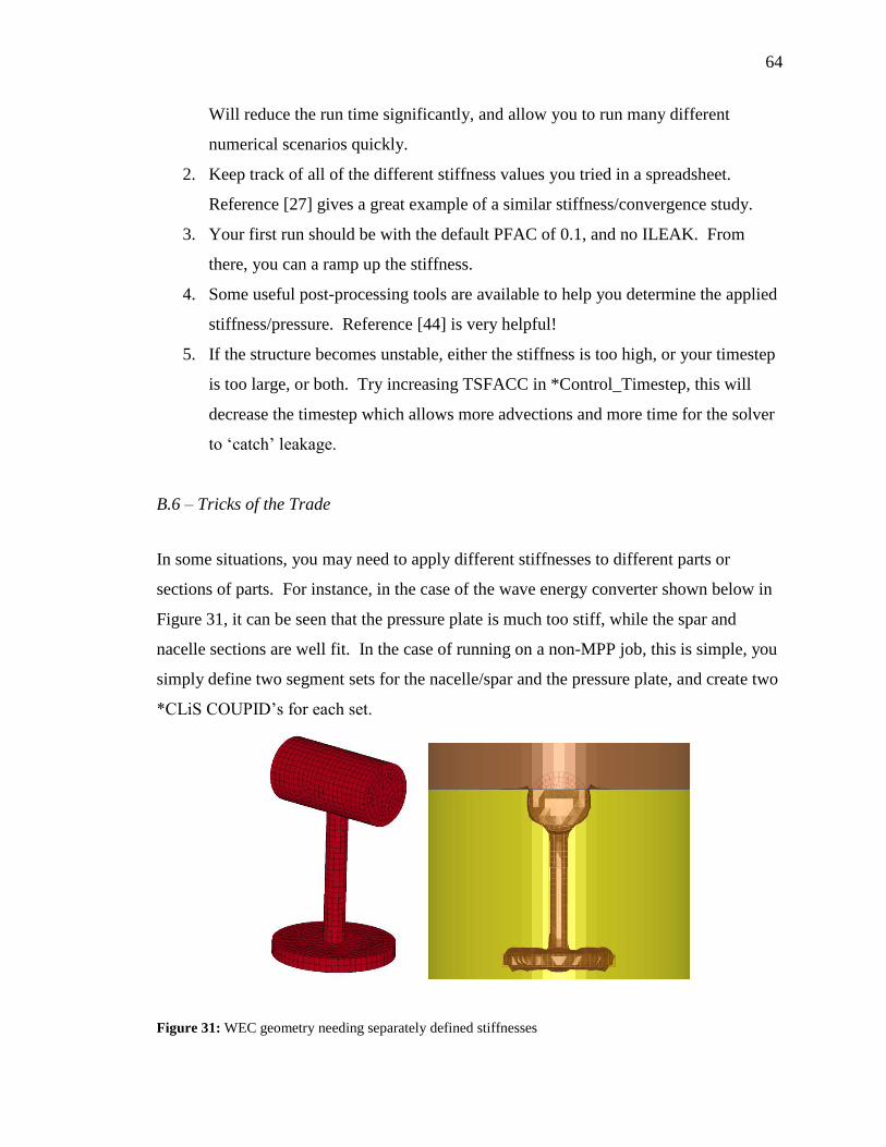
64
Will reduce the run time significantly, and allow you to run many different
numerical scenarios quickly.
2. Keep track of all of the different stiffness values you tried in a spreadsheet.
Reference [27] gives a great example of a similar stiffness/convergence study.
3. Your first run should be with the default PFAC of 0.1, and no ILEAK. From
there, you can a ramp up the stiffness.
4. Some useful post-processing tools are available to help you determine the applied
stiffness/pressure. Reference [44] is very helpful!
5. If the structure becomes unstable, either the stiffness is too high, or your timestep
is too large, or both. Try increasing TSFACC in *Control_Timestep, this will
decrease the timestep which allows more advections and more time for the solver
to „catch‟ leakage.
B.6 – Tricks of the Trade
In some situations, you may need to apply different stiffnesses to different parts or
sections of parts. For instance, in the case of the wave energy converter shown below in
Figure 31, it can be seen that the pressure plate is much too stiff, while the spar and
nacelle sections are well fit. In the case of running on a non-MPP job, this is simple, you
simply define two segment sets for the nacelle/spar and the pressure plate, and create two
*CLiS COUPID‟s for each set.
Figure 31: WEC geometry needing separately defined stiffnesses
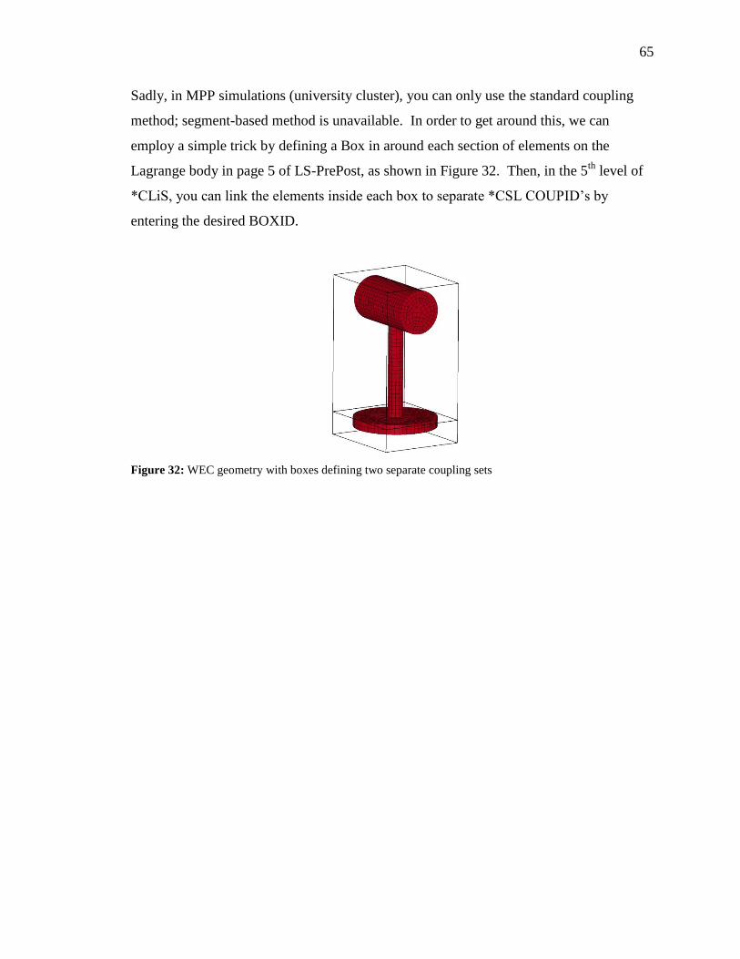
65
Sadly, in MPP simulations (university cluster), you can only use the standard coupling
method; segment-based method is unavailable. In order to get around this, we can
employ a simple trick by defining a Box in around each section of elements on the
Lagrange body in page 5 of LS-PrePost, as shown in Figure 32. Then, in the 5th
level of
*CLiS, you can link the elements inside each box to separate *CSL COUPID‟s by
entering the desired BOXID.
Figure 32: WEC geometry with boxes defining two separate coupling sets
66
Appendix C – Fast Gravity Application in LS-DYNA
Traditionally, gravity has to be applied in ALE FSI simulations over a large time period
(0.5 to 2 seconds), in order to prevent spurious oscillations in the fluid as a result of rapid
application of gravity. This can be computationally time consuming, and can be avoided
by using *Damping_Part_Mass to damp out oscillations in the fluid.
If we begin with a numerical basin filled with water and a floating body, we can speed up
the application of gravity to occur over 5 or more timesteps. As a result of this rapid
application of gravity, oscillations will appear in the water ALE elements. The amplitude
and period of the oscillations will be a function of the basin geometry, the water element
formulation (speed of sound, viscosity, etc.), and the „jerk,‟ the slope of the acceleration
curve.
The first step should be to apply „fast‟ gravity in the absence of any damping on the
water. This will allow you to examine the oscillations in the water, and to estimate the
necessary damping. By examining element solutions from the ASCII file, or the element
History in LS-PrePost, you can view the pressure history. Turning the dt up on the
*Dbase_History_Solid rather than the d3plot frequency will save a considerable amount
of hard drive space. Be sure that your dt on the d3plots/ ASCII is low enough to give
sufficient resolution. A crude estimation of the damping can be estimated by B=4*pi/T,
where T is the observed oscillation period.
Once you have estimated the damping, you can apply it by defining a load curve, and applying it
applying it in *Damping_Part_Mass. For example, if we apply gravity over 0.05 sec to a
cylindrical drop tank, from
Figure 33 we see pressure waves with a period of T~0.0169 seconds. From this, we apply
damping of B = 750, with a load curve as shown in Figure 34. In this load curve, the
damping is applied starting at t=0, and continues until >= 2*dtgrav, and then ramps down
to allow for the natural physics of the basin to take effect. Using this exact duration for
damping is not critical, you just need to hold the damping long enough to remove all of

67
the oscillations. Examining the pressure plots after the damping has been applied, we see
very little or no oscillations.
Figure 33: Pressure oscillations resulting from gravitational jerk
Figure 34: Damping curve for ALE water elements
68
Appendix D – Mooring Lines, Implementation of Cable Elements
This tutorial will explain how to implement cable elements with pretension, which can be
used for non-linear mooring lines. The element used is *Mat_071-
Cable_Discrete_Beam. The description of this element in the Keyword Manual is very
well written, and clearly details the materials functionality.
D.1 – Creating Beam Elements
The easiest way to create the beams is to use ElEdit in page 2 of LS-PrePost, and create a
starting node for the lines. After this, you can use ElGen, also on page 2 create a beam
via Node_drag. Another method is to define the starting and ending nodes of each line,
and then create a beam between the nodes. Of course, you can always drag node from a
preexisting structure. Note that you do not need a third node for this element, because it
is a 1-D discrete element.
D.2 – Defining the Loading Curve
For this material, you must define the load curve for engineering stress versus strain, not
force-displacement as used in other discrete elements. First, you should define the
*Mat_071-Cable_Discrete_Beam keyword, as shown in Figure 35. In this card, the
Young Modulus (E) is left blank - if a load curve is defined, this parameter is ignored. In
this instance, load curve 6 was used. If you do not specify a load curve, the cable stress is
determined using the linear relation Sigma = E*strain. From there, the force is
determined from F = Sigma / CA, where CA is the cross sectional area of the cable. The
CA is determined from the *Section_beam card, described later. F0 is the pretension for
the cable elements, and is applied at the first timestep in the simulation. TRAMP is
useful when bringing the system to equilibrium. If you don‟t define a ramp period, your
mooring system will „jerk‟ into tension at t=0, causing line oscillations. A good
technique is to define TRAMP during the application of gravity.
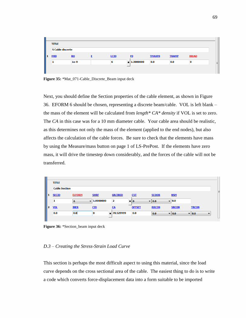
69
Figure 35: *Mat_071-Cable_Discrete_Beam input deck
Next, you should define the Section properties of the cable element, as shown in Figure
36. EFORM 6 should be chosen, representing a discrete beam/cable. VOL is left blank –
the mass of the element will be calculated from length* CA* density if VOL is set to zero.
The CA in this case was for a 10 mm diameter cable. Your cable area should be realistic,
as this determines not only the mass of the element (applied to the end nodes), but also
affects the calculation of the cable forces. Be sure to check that the elements have mass
by using the Measure/mass button on page 1 of LS-PrePost. If the elements have zero
mass, it will drive the timestep down considerably, and the forces of the cable will not be
transferred.
Figure 36: *Section_beam input deck
D.3 – Creating the Stress-Strain Load Curve
This section is perhaps the most difficult aspect to using this material, since the load
curve depends on the cross sectional area of the cable. The easiest thing to do is to write
a code which converts force-displacement data into a form suitable to be imported
70
directly into LS-PrePost. Shown below is an .m-file which does this. This code reads an
excel file containing Force-displacement data, and then converts it to stress-strain data.
This program assumes that the maximum displacement listed in the raw data is 100%
strain. Should the element stretch further, LS-DYNA will linearly extrapolate the next
points. The most important thing to note is that pretension should not be included in the
excel file, and should be input directly into the *Mat_071-Cable keyword.
An important thing to note is that LS-DYNA needs the first line entry in the tab-delimited
text file to be the number of data points to be read by the “Load XY Data” function. E.g.
if there are 9 stress strain points, the first line of the .txt file should be 9, which is
followed by the rest of the tab delimited pairs.
% file which produces a tab delimited file which can be read by LS-
Prepost % especially for cable elements, which require stress versus strain
load % curve input (other NL discrete elements use force-displacement)
%this file reads an excel file with the raw data and converts it into %stress strain data depending on the diameter %raw data: column 1 = displacement (mm), column 2 = tension (N)
%pretension should be neglected for this program, but input inside %*Mat_cable_discrete_beam
clear all close all clc
%=========================ENTER THESE VALUES
FIRST=========================
%Remeber consistent units between raw data and these parameters %standard units - N, mm, s, ton, Pa, etc.
directory = 'X:\Directory\mooring\’; filename = 'Raw_excel_data.xlsx';
data_name = 'Dyna_mooring.txt'; line_dia = 10; %======================================================================
==== xA = (pi/4)*(line_dia^2); %Cable cross sectional area
[rawdata] = xlsread(filename); %read in the excel file
71
len = length(rawdata); %the number of points in the raw data set
stress = rawdata(:,2)/xA; %stress = F/xA strain = rawdata(:,1)/rawdata(len,1); %strain =
displacement/Maxdisplacement
processed = zeros(len+1,2); %pre allocate the matrix processed(1,1) = len; %put length in first entry so LS-DYNA can read it processed(2:end,1) = strain; processed(2:end,2) = stress;
dlmwrite(data_name,processed,'delimiter','\t') %write the tab
delimited file
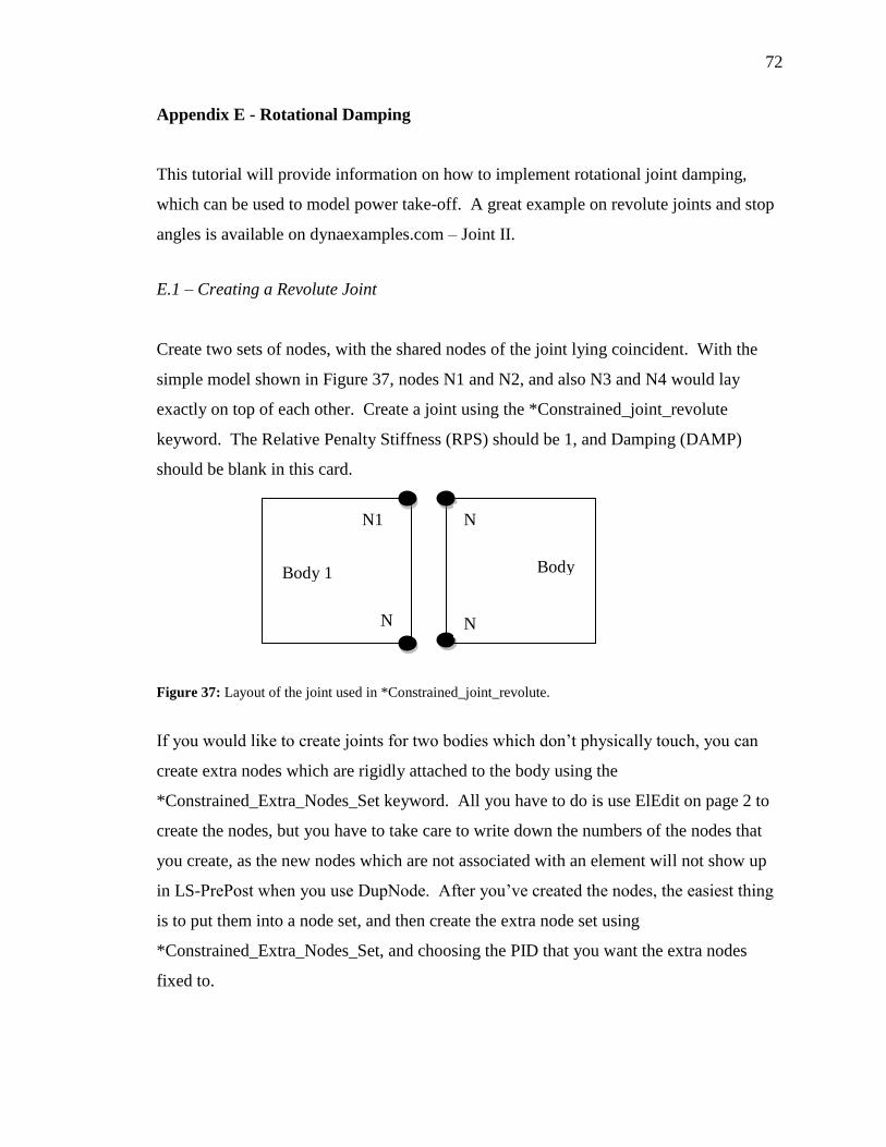
72
Appendix E - Rotational Damping
This tutorial will provide information on how to implement rotational joint damping,
which can be used to model power take-off. A great example on revolute joints and stop
angles is available on dynaexamples.com – Joint II.
E.1 – Creating a Revolute Joint
Create two sets of nodes, with the shared nodes of the joint lying coincident. With the
simple model shown in Figure 37, nodes N1 and N2, and also N3 and N4 would lay
exactly on top of each other. Create a joint using the *Constrained_joint_revolute
keyword. The Relative Penalty Stiffness (RPS) should be 1, and Damping (DAMP)
should be blank in this card.
Figure 37: Layout of the joint used in *Constrained_joint_revolute.
If you would like to create joints for two bodies which don‟t physically touch, you can
create extra nodes which are rigidly attached to the body using the
*Constrained_Extra_Nodes_Set keyword. All you have to do is use ElEdit on page 2 to
create the nodes, but you have to take care to write down the numbers of the nodes that
you create, as the new nodes which are not associated with an element will not show up
in LS-PrePost when you use DupNode. After you‟ve created the nodes, the easiest thing
is to put them into a node set, and then create the extra node set using
*Constrained_Extra_Nodes_Set, and choosing the PID that you want the extra nodes
fixed to.
Body 1
N
3
N
4
N
2
N1
Body
2
73
Be sure to define nodal masses for the extra node sets, and the masses you define are
realistic. F = m*a – If you don‟t define the nodal masses, the nodal forces will not be
transmitted.
E.2 – Applying Damping to the Joint
This procedure can be used to apply rotational damping or rotational springs to the joint
which you have previously created. Adding stop angles to the joint will also be covered
in this section.
Damping is easy to apply to a pre-existing revolute joint, without adding outside discrete
elements. The first step is to create the *Constrained_Joint_Stiffness_Generalized card, as
as shown in
Figure 38. Inside this card, you define the parts and their relative coordinate systems which
determine the joint forcing as a result of relative motion. In
Figure 38, rotational damping (load curve 10), has been applied between PIDA (part 1)
and PIDB (part 2). Be sure that your damping load curve is defined for both negative and
positive rotations. A coordinate system was defined for the two bodies using
*Define_Coordinate_Nodes. Since both of the coordinate systems coincide at t=0 and
there is no initial offset in nodal rotation, the same coordinate system can be used for
both bodies (CIDA=CIDB). Since there is only one joint in this particular simulation,
leaving JID (JID to which the damping and spring forces are applied) blank is
permissible.
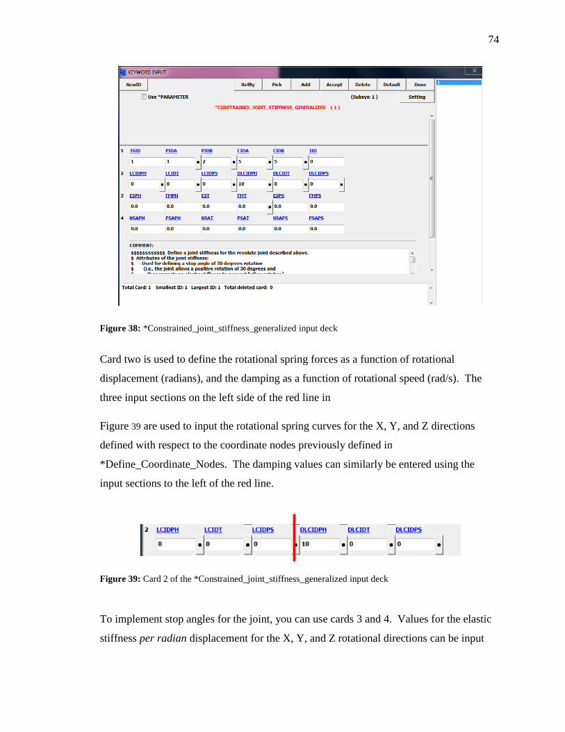
74
Figure 38: *Constrained_joint_stiffness_generalized input deck
Card two is used to define the rotational spring forces as a function of rotational
displacement (radians), and the damping as a function of rotational speed (rad/s). The
three input sections on the left side of the red line in
Figure 39 are used to input the rotational spring curves for the X, Y, and Z directions
defined with respect to the coordinate nodes previously defined in
*Define_Coordinate_Nodes. The damping values can similarly be entered using the
input sections to the left of the red line.
Figure 39: Card 2 of the *Constrained_joint_stiffness_generalized input deck
To implement stop angles for the joint, you can use cards 3 and 4. Values for the elastic
stiffness per radian displacement for the X, Y, and Z rotational directions can be input
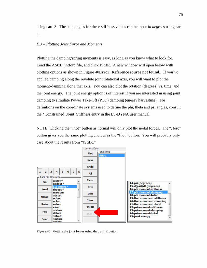
75
using card 3. The stop angles for these stiffness values can be input in degrees using card
4.
E.3 – Plotting Joint Force and Moments
Plotting the damping/spring moments is easy, as long as you know what to look for.
Load the ASCII_jntforc file, and click JStifR. A new window will open below with
plotting options as shown in Figure 40Error! Reference source not found.. If you‟ve
applied damping along the revolute joint rotational axis, you will want to plot the
moment-damping along that axis. You can also plot the rotation (degrees) vs. time, and
the joint energy. The joint energy option is of interest if you are interested in using joint
damping to simulate Power Take-Off (PTO) damping (energy harvesting). For
definitions on the coordinate systems used to define the phi, theta and psi angles, consult
the *Constrained_Joint_Stiffness entry in the LS-DYNA user manual.
NOTE: Clicking the “Plot” button as normal will only plot the nodal forces. The “Jforc”
button gives you the same plotting choices as the “Plot” button. You will probably only
care about the results from “JStifR.”
Figure 40: Plotting the joint forces using the JStiffR button.

76
Appendix F – Writing, Extracting, and Plotting LS-DYNA Result Files
This tutorial starts with general information on writing and extracting ASCII/binout files.
The second section provides information on how to extract and plot the FSI force for
ALE coupling, which requires a different procedure.
F.1 – Writing and Extracting
In LS-PrePost version 970 and above, the ASCII files are not printed directly, even if you
select them in the *Dbase_ASCII_option option by checking the appropriate ASCII
option, entering dt, and choosing options 1, 2 or 3 for output. Instead, the program
outputs binout file(s), which contain all of the information which you selected in the
ASCII_option card. It is advisable to use the *Control_MPP_IO_BINOUTONLY card.
In order to print or save the individual ASCII_options contained within the binout file(s),
follow the procedure below. It is followed by a LS-PrePost screenshot to help show
locations in the GUI in Figure 41:
1) Open the d3plot file in LS-PrePost
2) Under page 2, click the Binout button in the upper right (letter A).
3) The “Open Files” window will appear in the lower left of the screen. Load the
binoutXXXX file (letter B). The checked outputs from the ASCII_option card
should show directly to the right of the load window (Letter C). Click “Save.”
4) On the same screen on the middle right side in the “Output Interface”, all of the
data for the ASCII_option(s) should appear under “Write out branches (letter D).”
Click “All” to select all of the ASCII cards, and then check “As ASCII(es).”
5) Click the “Apply” button below (letter E). All of the ASCII output files will be
saved in the directory where the d3plot files are stored.
6) If you go back to page 1, you now should be able to plot all of the ASCII_options.
If you only want to plot the results in the binout file (not save the individual ASCII
outputs), then you can load the file as in step 3 above, but then click on the desired option

77
directly to the right of the open file in the lower part of the screen. From there, you can
select the nodes, bodies, etc. to plot using the three sections on the right of the screen.
Another note: You must sometimes activate other cards within *Dbase to tell LS-PrePost
which nodes or elements, etc. you want to include in the binout (or ASCII) outputs. For
instance, if you want to output the nodal forces using *Dbase_ASCII_NODOUT, you
must also use the *Dbase_nodal_force_group card to define the included nodes.
Figure 41: LS-PrePost GUI with locations used for extracting ACSII binout files.
F.2 – Plotting FSI Forces
Knowledge of the FSI coupling force is one of the most important steps towards
determining correct coupling parameters. There are several steps that you must take to
have the dbfsi files output by LS-DYNA. The first step is to tell LS-DYNA that you
want the FSI force available for writing by the *Dbase card. Do this by opening
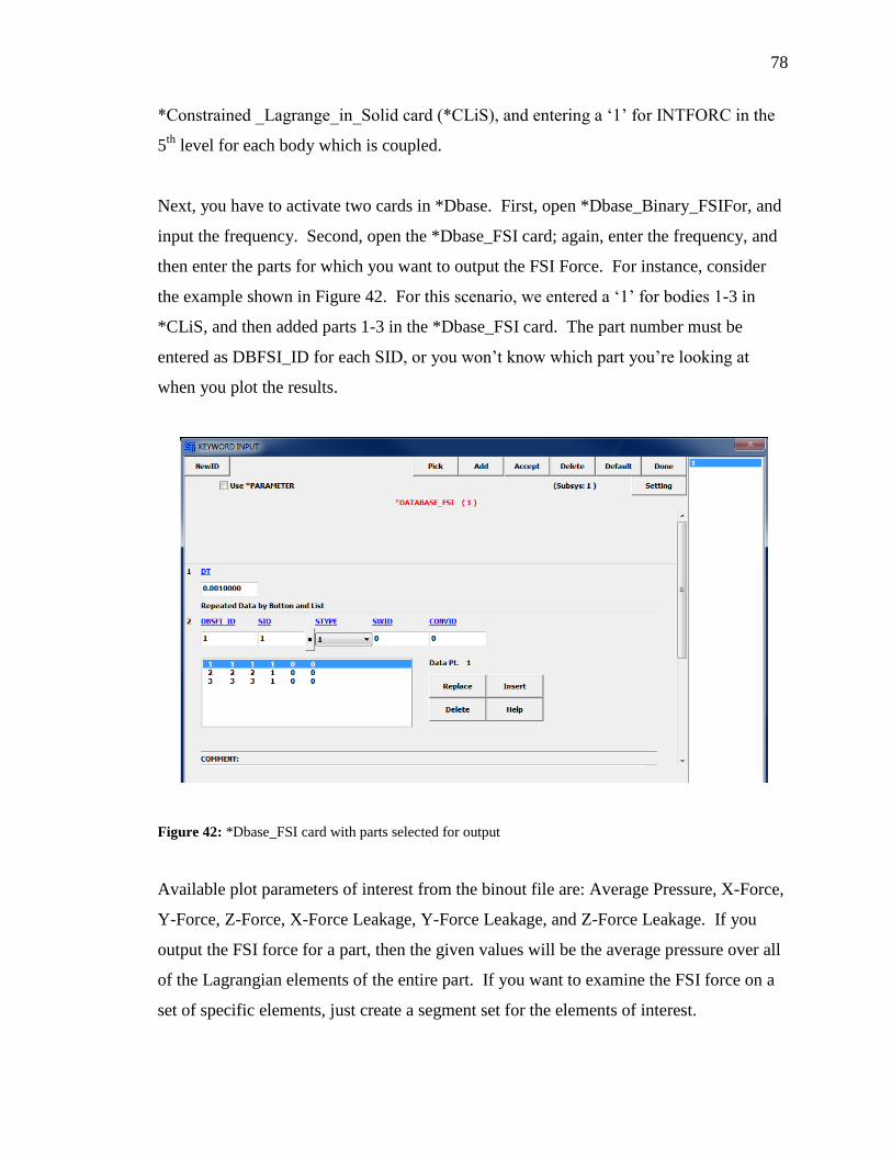
78
*Constrained _Lagrange_in_Solid card (*CLiS), and entering a „1‟ for INTFORC in the
5th
level for each body which is coupled.
Next, you have to activate two cards in *Dbase. First, open *Dbase_Binary_FSIFor, and
input the frequency. Second, open the *Dbase_FSI card; again, enter the frequency, and
then enter the parts for which you want to output the FSI Force. For instance, consider
the example shown in Figure 42. For this scenario, we entered a „1‟ for bodies 1-3 in
*CLiS, and then added parts 1-3 in the *Dbase_FSI card. The part number must be
entered as DBFSI_ID for each SID, or you won‟t know which part you‟re looking at
when you plot the results.
Figure 42: *Dbase_FSI card with parts selected for output
Available plot parameters of interest from the binout file are: Average Pressure, X-Force,
Y-Force, Z-Force, X-Force Leakage, Y-Force Leakage, and Z-Force Leakage. If you
output the FSI force for a part, then the given values will be the average pressure over all
of the Lagrangian elements of the entire part. If you want to examine the FSI force on a
set of specific elements, just create a segment set for the elements of interest.


![[Robert K. Ritner] Libyan Anarchy. Inscriptions Fr(BookFi.org)](https://static.fdocuments.us/doc/165x107/55cf9a1d550346d033a08592/robert-k-ritner-libyan-anarchy-inscriptions-frbookfiorg.jpg)


