The predictive qualities of earnings volatility and earnings uncertainty

Dain C. Donelson

McCombs School of Business, University of Texas at Austin

2110 Speedway Avenue, B6400

Austin, TX 78712

dain.donelson@mccombs.utexas.edu

Phone: (512) 232-3733 Fax: (512) 471-3904

Robert J. Resutek †

Tuck School of Business – Dartmouth

100 Tuck Hall

Hanover, NH 03755

robert.j.resutek@tuck.dartmouth.edu

Phone: (603) 646-9635 Fax: (603) 646-1698

Abstract

This study examines the differential predictive power of past earnings volatility for analyst forecast errors and

future returns. Past earnings volatility jointly captures two correlated, but distinct, earnings properties: time-

series earnings variation and uncertainty in future earnings. To distinguish between these two earnings

properties, we develop a forward-looking measure of earnings uncertainty that has a minimal mechanical link

to variation in prior period earnings realizations and does not rely on analyst forecasts. Our collective results

suggest that future earnings uncertainty, and not time variation in earnings, is associated with overly-optimistic

future earnings expectations of equity analysts and investors. We provide the first empirical evidence on the

relevance of future earnings uncertainty to analysts and investors over one-year horizons. In addition, we

provide empirical evidence showing that forecast dispersion is a poor measure of earnings uncertainty.

JEL Codes: G14, M41

Key Words: Earnings Volatility, Information Uncertainty, Earnings Prediction, Analyst Forecasts, Asset

Pricing

Data Availability: Data is available from public sources as identified in the text.

† Contact author. We thank Andy Bernard, Steve Kachelmeier, Chad Larson, Shai Levi, Jonathan Lewellen,

Matt Lyle, John McInnis, Phil Stocken and workshop participants at Dartmouth (Tuck School of Business),

2011 American Accounting Association annual meeting, the University of Mississippi and the University of

Texas at Austin for helpful comments.

The predictive qualities of earnings volatility and earnings uncertainty

This study examines the differential predictive power of past earnings volatility for analyst forecast errors and

future returns. Past earnings volatility jointly captures two correlated, but distinct, earnings properties: time-

series earnings variation and uncertainty in future earnings. To distinguish between these two earnings

properties, we develop a forward-looking measure of earnings uncertainty that has a minimal mechanical link

to variation in prior period earnings realizations and does not rely on analyst forecasts. Our collective results

suggest that future earnings uncertainty, and not time variation in earnings, is associated with overly-optimistic

future earnings expectations of equity analysts and investors. We provide the first empirical evidence on the

relevance of future earnings uncertainty to analysts and investors over one-year horizons. In addition, we

provide empirical evidence showing that forecast dispersion is a poor measure of earnings uncertainty.

1. Introduction

This study investigates the predictive power of past earnings volatility to explain the forecast errors of equity

analysts and investors. Past earnings volatility, defined as the standard deviation of past earnings realizations,

jointly captures two distinct economic constructs: time variation in earnings and the precision with which

future earnings can be estimated. By time-variation in earnings, we mean the time-series volatility in earnings

realizations caused by accrual measurement errors and fundamental economic shocks (Dichev and Tang 2009).

By precision, we mean how precisely future earnings as reported under GAAP can be estimated in the current

period. In this study, we refer to earnings precision in terms of its inverse, earnings uncertainty, and define it

as the distribution around future earnings expectations. We disentangle these two correlated economic

constructs captured by past earnings volatility and determine their relative predictive power for explaining the

forecast errors of equity analysts and investors.

The primary motivation for our study stems from the fact that despite a relatively extensive literature

examining the consequences of past earnings volatility, prior studies have not investigated whether historical

variation in earnings is relevant to analysts and investors once earnings uncertainty (the precision with which

future earnings can be estimated) has been controlled. Graham et al. (2005) note executives strongly believe

more volatile earnings are less predictable and less predictable earnings have negative consequences. However,

as noted by Dichev and Tang (2009), it is unclear whether managers dislike past earnings volatility because

they believe time-variation in earnings directly leads to more uncertain future earnings or if managers dislike

uncertain future earnings (which happen to be correlated with a volatile past earnings stream). Carrying

forward this question to the broader accounting literature, it is unclear whether variation in past earnings

affects the earnings forecasts of analysts and investors after controlling for the effect of earnings uncertainty.

This question is important as a primary tension in the accounting literature lies in understanding whether

actions (and reactions) of analysts and investors prior studies associate with past earnings volatility are due to:

i) the underlying uncertainty of future earnings, or ii) the way past earnings were reported between t-τ and t.

The primary challenge in separating the predictive power associated with time-series earnings variation from

2

that associated with earnings uncertainty comes from the tight connection between the two constructs. Indeed,

time variation in earnings, measured by past earnings volatility, is often used to proxy for earnings uncertainty

as firms with more volatile earnings processes tend to have future earnings that are more difficult to predict

(e.g., Dichev and Tang 2009). At the same time, however, realized earnings variation and earnings uncertainty

are not perfectly linked. For example, extreme earnings realizations will increase past earnings volatility, but

may not increase the uncertainty of future earnings because extreme earnings tend to (predictably) mean revert

very quickly. Further, earnings realizations from early periods will affect past earnings volatility, but may be

unrelated to the predictability of future earnings since these realizations no longer convey timely information.

To distinguish the incremental predictive power of the two accounting constructs captured by past earnings

volatility, earnings uncertainty and time variation in earnings, we develop a novel, firm-specific measure of

earnings uncertainty that has a minimal mechanical link to time variation in earnings and is not derived from

analyst earnings forecasts. Our measure builds on Barber and Lyon (1996) and Blouin et al. (2010) and uses a

matched-firm expectation model to estimate future earnings and the uncertainty associated with the future

earnings expectation.

Our central empirical result strongly suggests that earnings uncertainty, and not time-series earnings variation,

predicts forecast errors of equity analysts and investors. Using conventional cross-sectional regressions, we

find that earnings uncertainty significantly predicts future returns: controlling for size, book-to-market,

accruals, and momentum, average predictive slopes for future monthly returns on earnings uncertainty are

negative and three to five standard errors from zero, depending on the specification. We find similar predictive

inferences, both in statistical and economic terms, on earnings uncertainty using hedge return portfolio tests

and analyst forecast errors. Collectively, our empirical results suggest that earnings uncertainty, and not time-

variation in earnings, has significant predictive power for the errors of analysts and investors.

In addition, we find past earnings volatility, but not earnings uncertainty, strongly predicts lower future

earnings. Our results confirm the conjecture that time-variation in earnings lead to lower future earnings

3

(Minton, Schrand, and Walther 2002), suggesting time-variation in earnings has real effects on future firm

performance. However, our evidence suggests analysts and investors understand these effects once earnings

uncertainty is controlled.

Our study contributes to the accounting and finance literatures in three additional ways. First, we propose and

validate a forward-looking, firm-specific measure of earnings uncertainty. Our measure requires a minimal

time-series of earnings realizations, thereby minimizing the mechanical relation with past earnings volatility.

In specification tests, we show that this measure is well specified in the full sample and in select subsamples of

firms experiencing extreme performance. Further, in direct comparative tests, we show our uncertainty

measure better estimates earnings uncertainty (more precise and less biased) compared to estimates derived

from analyst forecast dispersion. Our uncertainty measure offers future researchers not only a better estimate

of uncertainty, but also one available for a broader number of firms spanning a longer time-series.

Second, our results contribute to the information uncertainty and the ‘low volatility’ anomaly literatures

(Zhang 2006; Baker et al. 2011). Prior studies in these literatures do not directly articulate the source of

investor uncertainty. Rather, these literatures proxy for uncertainty using variables that jointly capture

multiple types of uncertainty and future expected performance.1 Our results suggest earnings uncertainty is a

significant predictor of future returns over horizons extending at least 12 months, a result that counters the one

to three month predictive relations noted in prior studies (Diether et al. 2002; Ang et al. 2006).

Third, while not the primary purpose of our study, we also contribute to the earnings prediction literature.

While accounting researchers have produced an extensive set of earnings prediction models, the models are

primarily derived from ordinary least squares regressions and therefore subject to the restrictions and

assumptions imposed by OLS. We extend the work of Barber and Lyon (1996) and show that our

nonparametric matched-firm empirical design produces superior earnings expectations relative to simpler

1 For example, firm size, market-to-book, forecast dispersion, realized return volatility (and other variables) have

each been used as empirical proxies for information uncertainty.

4

random walk and analyst forecast prediction models for a broad set of firms. Barber and Lyon (1996) primarily

examine operating earnings of NYSE and AMEX firms from 1977-1992 whereas we examine earnings before

extraordinary items of NYSE, AMEX, and NASDAQ firms from 1968-2009.

The rest of our study proceeds as follows. Section 2 discusses prior literature and motivates our research

question and empirical tests. Section 3 describes our measure of earnings uncertainty and the construction of

our primary sample. Sections 4 and 5 report results from our primary empirical tests. Section 6 reports

robustness tests. Section 7 concludes.

2. Research Motivation

2.1 Prior literature and empirical design

Prior studies in accounting and finance have differed in their interpretation of past earnings volatility and why

it is (or is not) relevant to capital market participants. Many studies interpret past earnings volatility as an

empirical measure capturing value-irrelevant noise caused by measurement error in the accrual process and

transitory economic shocks (e.g., Dichev and Tang 2009), linking it to a series of negative firm outcomes.

These negative firm outcomes include biased analyst earnings forecasts (Dichev and Tang 2009), analyst

coverage effects (Lang, Lins, and Miller 2003), higher cost of equity capital (Francis et al. 2004; 2005).

Related studies find time variation in cash flows affects investment decisions, leading to lower investment and

lower future earnings (Minton and Schrand 1999; Minton, Schrand and Walther 2002). Finally, similar in

tenor to the volatility literatures, the earnings smoothness literature views past earnings volatility as a measure

of the discretionary reporting choices made by managers to smooth reported earnings. The primary debate in

the earnings smoothness literature is whether the discretionary reporting choices made by managers over time

clarify or garble the informativeness of earnings (Tucker and Zarowin 2006; Jayaraman 2008; Rountree et al.

2008).2 While the research designs and research questions vary across these (and other) studies examining past

earnings volatility, the general takeaway is fairly consistent: the significant associations between past earnings

2 Dechow, Ge, and Schrand (2010) provide a more extensive discussion on the earnings smoothness literature within

the broader context of earnings quality.

5

volatility and a series of negative firm outcomes suggests that time-variation in earnings is relevant to a large

set of capital market participants and an undesirable earnings attribute.

An alternative perspective suggests the precision with which future earnings can be estimated, not time-

variation in earnings, is the primary economic dynamic behind the significant associations with past earnings

volatility documented in prior studies. This view is emphasized in early accounting studies examining the link

between accounting measures of risk and market measures of risk (Beaver, Kettler, and Scholes 1970;

Rosenberg and McKibben 1973). It also is consistent with more recent studies that suggest the precision with

which future earnings and cash flows can be estimated affects firm value, either because the precision of

earnings estimates affects a firm’s cost of capital (Easley and O’Hara 2004; Johnson 2004; Lambert, Leuz and

Verrecchia 2007) or variation in investors’ assessment of earnings precision affects their expectations of future

earnings (Daniel, Hirshleifer and Subrahmanyam 1998; Jiang et al. 2005).

Obviously, there is significant conceptual overlap between the two interpretations of past earnings volatility.

Firms with more volatile historical earnings streams will tend to have future earnings that are more uncertain.

Thus, the use of past earnings volatility as an empirical proxy for uncertainty in future earnings is reasonable

as the two constructs, time-variation in earnings and earnings uncertainty, are certainly positively correlated.

However, the conceptual overlap between the two constructs is not complete and, in fact, the two constructs

are expected to diverge from each other in predictable ways. For example, timely loss recognition associated

with accounting conservatism is one reason we might observe a negative correlation between past earnings

volatility and earnings uncertainty (Frankel and Litov 2009). Relatedly, large losses tend to be transitory and

are associated with strong earnings reversals in the subsequent period. Nonetheless, large one-time losses will

lead to higher past earnings volatility, though not necessarily high earnings uncertainty (especially the earlier

in the time-series the one-time loss is recognized). Another example is noted by Kothari et al. (2002), who

find research and development expenditures are positively associated with earnings volatility even though

R&D leads to predictably higher future earnings (Lev and Sougiannis 1996).

6

Understanding whether time-variation in earnings (a function of past economic shocks and manager reporting

choices) affects the earnings forecasts of analysts and investors incremental to contemporaneous earnings

uncertainty serves as the primary motivation for our study. Prior studies examining past earnings volatility and

earnings quality suggest financial reporting choices have significant consequences incremental to the economic

performance captured by earnings. However, prior studies have been unable to determine whether the

consequences associated with past earnings volatility are due to contemporaneous earnings uncertainty at time

t or uncertainty caused over time (because past earnings volatility is a joint function of past economic shocks

and measurement errors inherent in the accrual system, and each element is likely correlated with future

earnings uncertainty).

In the subsequent sections, we briefly discuss the two modal empirical variables used in prior studies to proxy

for earnings uncertainty: past earnings volatility and analyst forecast dispersion. We discuss the strengths and

weaknesses of each variable and then propose a potential alternative empirical proxy for earnings uncertainty.

We highlight its empirical costs and benefits relative to past earnings volatility and analyst forecast dispersion.

We then provide our empirical predictions.

2.2 The relation between past earnings volatility and earnings uncertainty

If a firm’s earnings process is reasonably stable, then past earnings volatility (as measured by variation in a

time series of realizations) will be a precise and unbiased estimate of uncertainty in future earnings. However,

to the extent each earnings realization in the time-series is not equally informative of the underlying future

earnings process of the firm, past earnings volatility will not proxy for earnings uncertainty. Further, as noted

by Frankel and Litov (2009), some accounting conventions such as conservatism will lead to more volatile

earnings process while at the same time (possibly) producing less uncertain future earnings. Accordingly, we

expect that past earnings volatility is positively correlated with earnings uncertainty for the average firm.

However, for any given firm, the strength and sign of these associations could vary significantly.

7

2.3 The relation between analyst forecast dispersion and earnings uncertainty

The dominant empirical measure of earnings uncertainty in the accounting and finance literature is dispersion

in analyst forecasts.3 Advantages of this measure include the fact that dispersion is a direct function of an

earnings expectation model (i.e., it represents a distribution around an expected value, the consensus forecast),

it is not a mechanical function of prior period earnings realizations, and earnings expectations are routinely

updated in response to news.

Nonetheless, the use of analyst forecasts has several costs. Analyst forecasts are only available in machine

readable format for relatively large, mature firms and coverage is relatively sparse for even large firms prior to

1990. Second, analyst earnings forecasts are not consistently defined across firms or even across firms in the

same industry as analysts exclude line items inconsistently (Brown and Larocque 2013). Third, analyst

forecasts are biased, although the direction of the bias is context-specific which leads to more empirical

complications.4 Consideration of these biases is important since earnings uncertainty represents the second

moment of earnings; thus, proxies for earnings uncertainty will only be as good as the empirical proxies for the

first moment (i.e., the earnings expectation). Finally, as McNichols and O’Brien (1997) and Diether et al.

(2002) point out, the analysts’ incentives to cover a firm may directly affect both the consensus forecast and

the dispersion. For example, analysts are much more likely to drop the coverage of a firm they view negatively

than to formally issue a negative forecast. Performance-related censoring of the available forecasts can lead to

optimistic biases in earnings forecasts and understated estimates of earnings uncertainty for poorly performing

firms. While the optimistic earnings expectation bias is well documented, whether forecast dispersion is an

unbiased estimate of earnings uncertainty has not been directly examined in prior studies.

3 Analyst forecast dispersion is sometimes also referred to as opinion divergence (Diether et al 2002). Alternative

measures of earnings uncertainty based on forecast dispersion exist in the literature. Barron, Kim, Lim, and Stevens

(1998) suggest a measure that decomposes forecast dispersion into an uncertainty component and an information

asymmetry component. Sheng and Thevenot (2011) suggest an uncertainty measure based on a GARCH model. We

do not directly consider these alternative measures in our study as the BKLS model imposes a significant look-ahead

bias in its design by requiring the earnings realization to compute earnings uncertainty. The empirical design of

Sheng and Thevenot requires a significant time-series of forecasts (20+ years of earnings estimates per firm). 4 For example, analyst forecasts tend to be optimistically biased early in the fiscal period, pessimistically biased by

the end of the fiscal period. Analyst forecasts tend to be optimistically biased for “growth” firms, pessimistically

biased for “value” firms.

8

2.4 Motivation for a pure earnings uncertainty measure

The above discussion provides suggestive intuition as to why it is difficult to determine whether predictive

relations noted in prior studies on past earnings volatility or forecast dispersion are due to the time variation in

earnings, analyst coverage and forecast biases, or simply due to earnings uncertainty. Further convoluting any

analysis, if time variation in earnings affects analyst forecasts, then forecast dispersion could also jointly

capture dynamics associated with time-series earnings variation and earnings uncertainty.

To directly distinguish the predictive power of earnings uncertainty from time-variation in earnings, we need

to develop an empirical estimate of earnings uncertainty with a minimal mechanical relation to past earnings

realizations and one that does not require analyst forecasts. Specifically, we propose an earnings uncertainty

measure that builds on Barber and Lyon (1996). Barber and Lyon propose a nonparametric matched-firm

approach to estimate expected operating performance. Their empirical design is based on matching firm i at

time t to firms with comparable characteristics in the preceding period, yielding a firm-specific estimate of

expected future operating performance. If the firms that are matched to each firm i are reasonably comparable

to firm i in their earnings processes, then each matched firm’s realized earnings can be interpreted as a possible

earnings realization for firm i. Thus, similar to using the average analyst forecast to proxy for the consensus

expected earnings, Barber and Lyon find that expected earnings estimated as the average earnings of the

matched firms is a reasonable proxy for expected future earnings of the firm of interest.

Also produced from their empirical design, but unexplored by prior studies, is the empirical distribution of the

earnings realizations in period t of firm i's matched-firms. Specifically, since the matched-firms are grouped

together because they have characteristics similar to firm i, differences in the matched-firms’ earnings

realizations represent possible earnings realizations of firm i in period t+1. Accordingly, the standard deviation

of the matched-firms’ earnings realizations in period t can be viewed as the standard deviation (i.e., earnings

9

uncertainty) of firm i's expected t+1 earnings as of time t.5 Again, the intuition is similar to that used in the

analyst forecast literature: assuming the earnings process of each matched-firm is similar to the earnings

process of firm i, the standard deviation of possible earnings realizations for firm i serves as an inverse proxy

for how precisely future earnings can be estimated. Perhaps more importantly, the matched-firm uncertainty

measure has a minimal mechanical link to time-series earnings variation – exactly what we need for our

empirical tests to distinguish between earnings uncertainty and time-series variation in earnings.6

2.5 Matched-firm characteristics

The objective of the matched-firm empirical design is to couple firms from prior periods with similar earnings-

predictive characteristics to firm i. If the firms from prior periods that are matched to firm i have similar

earnings processes to firm i, their realized earnings changes will be reasonable t+1 expected earnings changes

for i. We base our matched-firm empirical design on three firm characteristics prior studies suggest are strong

predictors of future profits: current profits, one-year change in profits, and firm size.7

There is extensive empirical evidence in the accounting and finance literatures that profits are reasonably

persistent (Ball and Watts 1972; Watts and Leftwich 1977; Sloan 1996). That is, for the ‘average’ firm,

current earnings are a reasonable estimate of future earnings. Support for earnings persistence stems from the

microeconomics literature which suggests firms earn a return equal to the required return for the risk assumed.

Thus, assuming the ‘average’ firm is operating in a competitive industry, we expect the level of current

profitability to be predictive of subsequent period profitability.

While firm profitability is persistent, prior studies also note changes in profitability are predictive of future

5 Blouin et al. (2010) utilize similar intuition to project the distribution of pretax income level for twenty years to

estimate marginal tax rates. However, they do not project firm-specific estimates of earnings uncertainty nor explore

the capital market implications for the earnings volatility literature. 6 A more subtle advantage of using a matched-firm empirical design to estimate earnings uncertainty is that it side-

steps the tricky interpretive issues of using forecast dispersion which can also be interpreted as a measure of opinion

divergence associated with information asymmetry. 7 Consistent with prior earnings volatility studies , our ‘earnings’ variable is actually earnings scaled by average total

assets. We use terms earnings, profits, and profitability interchangeably.

10

earnings changes (Beaver 1970; Freeman, Ohlson, Penman 1982; Fama and French 2000). Again,

microeconomic theory provides the structure for understanding the predictive power of the earnings change

element: assuming firms operate in competitive industries, firms realizing higher earnings will face increased

competitive pressure from other firms, leading to lower earnings in the future.

Finally, while support of the importance of current profits and profit changes in the prediction of next year’s

earnings dates back many decades, our third firm characteristic, firm size, is based on more recent empirical

evidence. Fama and French (2004) note the earnings processes of smaller firms have become more volatile

and left-skewed beginning in the early 1980s. Since ‘small’ firms currently comprise a disproportionate

percentage of publicly traded firms in any given year and extreme earnings realizations are much less likely for

larger firms, we also use firm size as a partitioning matching variable.8

In sum, the matched-firm empirical design uses firms from prior periods with three firm characteristics that

closely mirror those of firm i in the current period. If the earnings processes in prior periods of the matched

firms are similar to those of firm i in the current period, each matched firm’s earnings realization will be a

reasonable possible earnings realization for firm i in the next period. Thus, similar to individual analyst

forecasts, the average matched firm earnings change can be interpreted as the ‘consensus’ expected earnings

change of firm i while the volatility in the earnings changes can be interpreted as an inverse measure of how

precisely future earnings can be estimated.

There are costs and benefits to our matched-firm approach. With respect to potential benefits, our matched-

firm process does not impose any structural relation between firm characteristics and earnings uncertainty

across time or across firms. In addition, the matched-firm approach is parsimonious, requiring a very limited

time-series of earnings realizations and firm characteristics thereby allowing estimates of earnings uncertainty

for a large subset of firms. However, the matching process requires an appropriate number of matched firms to

8 In the last year of our sample (2010), ‘small’ firms, which we define as having average total assets below the 10

th

NYSE-based total asset percentile, constituted 48% of our sample but less than 2% of the total market capitalization.

11

produce an earnings distribution. Since firms with extreme characteristics could have extreme earnings

uncertainty, these observations may tend to be omitted due to a lack of firms with comparable characteristics

or be estimated less precisely than firm-year observations with more matches.

In subsequent sections, we more precisely explain the mechanics of our matching criteria. More importantly,

we perform a series of specification tests to assess the validity of our earnings uncertainty measure. Our

specification tests examine the construct validity of our empirical earnings uncertainty estimate across a

variety of tests. If these tests suggest that our earnings uncertainty variable is reasonably well-specified, we

will be able to directly test the incremental predictive power of earnings uncertainty against time-series

variation in earnings (as captured by past earnings volatility).

III. Sample selection and variable measurement

3.1 Sample Selection

Our primary sample is drawn from the population of all firms listed in the Compustat Annual Industrial and

Research files. Since the primary variables of interest are earnings uncertainty and past earnings volatility, our

sample spans fiscal year ends 1968:06 – 2011:05. We define earnings as earnings before extraordinary items

(IB), scaled by average total assets (AT). We further reduce the sample to firms traded on the NYSE, AMEX,

and NASDAQ (CRSP exchange code 1, 2, 3), nonfinancial firms (exclude firms with SIC codes 6000-6999 per

CRSP), firms with CRSP share codes equal to 10, 11 and 12 and firms with non-missing earnings in t and t+1.

Our primary sample is comprised of all firms meeting the above criteria and have a calculable earnings

uncertainty value or a past earnings volatility measure, yielding 152,710 firm year observations.

3.2 Earnings uncertainty measurement

For each firm i at time t, we use as matched-firms all firms of similar size, earnings, and one-year earnings

change in any of the years t-5 to t-1. Specifically, each firm i is matched to firms in years t-5 to t-1 that are in

the same NYSE-based total asset portfolio. The first portfolio comprises all firms with total assets below the

10th NYSE-based asset percentile; all remaining firms fall in the second portfolio. Within each size portfolio,

12

firm i is subsequently matched to firms with comparable earnings and one-year earnings change. Consistent

with prior studies, we define earnings as earnings before extraordinary items scaled by average assets (Dichev

and Tang 2009). We define firms with comparable earnings and one-year earnings change to firm i at time t as

those firms whose t-τ earnings and t-τ one-year change in earnings are no more or less than 0.5 percent of firm

i's earnings and one-year earnings change in fiscal year t. This matching process yields, for each firm i, a set

of firms with comparable earnings performance observable at time t.9

For each of the matched firms, we compute the change in earnings between t-τ and t-τ+1. To reduce the

mechanical effect extreme earnings changes in a matched-firm can have on estimates of earnings uncertainty,

we discard matched-firms with extreme performance, defined as one-year change in earnings greater in

absolute magnitude than 50% of total assets.10

We use the average change in earnings across matched-firms as

firm i's expected earnings change between t and t+1. We use the standard deviation of the realized earnings

changes of the matched firms as a measure of firm i's earnings uncertainty around its t+1 earnings expectation.

We require at least five matches for each firm to compute this characteristic.

We repeat the matching procedure detailed above for all firms without at least five matches. Unmatched firms

tend to be those with more extreme current earnings or one-year earnings changes. For these firms, we utilize

a percentile-based matching procedure and use all firms within the same t-τ size portfolio whose t-τ earnings

and t-τ earnings change are between 80% and 120% of firm i’s earnings and one-year earnings change.11

As a result of our matched-firm expectation model, for each firm i, we have an expectation of t+1 earnings and

an estimate of the uncertainty surrounding each earnings expectation. Note, the matching process should

9 For example, IWKS (F/Y/E 1997) had earnings of 0.076, change in earnings of 0.032, and total assets below the

10th

NYSE total asset percentile. All firms with total assets below the 10th

NYSE total asset decile in fiscal years

1992-1996, with earnings between 0.071 and 0.081 and one-year change in earnings between 0.027 and 0.037 serve

as IWKS’s matched-firms. (In our sample, IWKS1997 had 20 matched firms). 10

This screen has a minimal effect on the average number of matched firms per firm (less than 1 percent). 11

For example, ALGI (F/Y/E 1996) had earnings of 0.114, change in earnings of -0.082, and total assets below the

10th

NYSE total asset percentile. All firms with total assets below the 10th

NYSE percentile in fiscal years 1991-

1995, earnings between 0.091 and 0.137, and one-year change in earnings between -0.066 and -0.098 serve as

ALGI’s matched-firms. (In our sample, ALGI1996 had 28 matches).

13

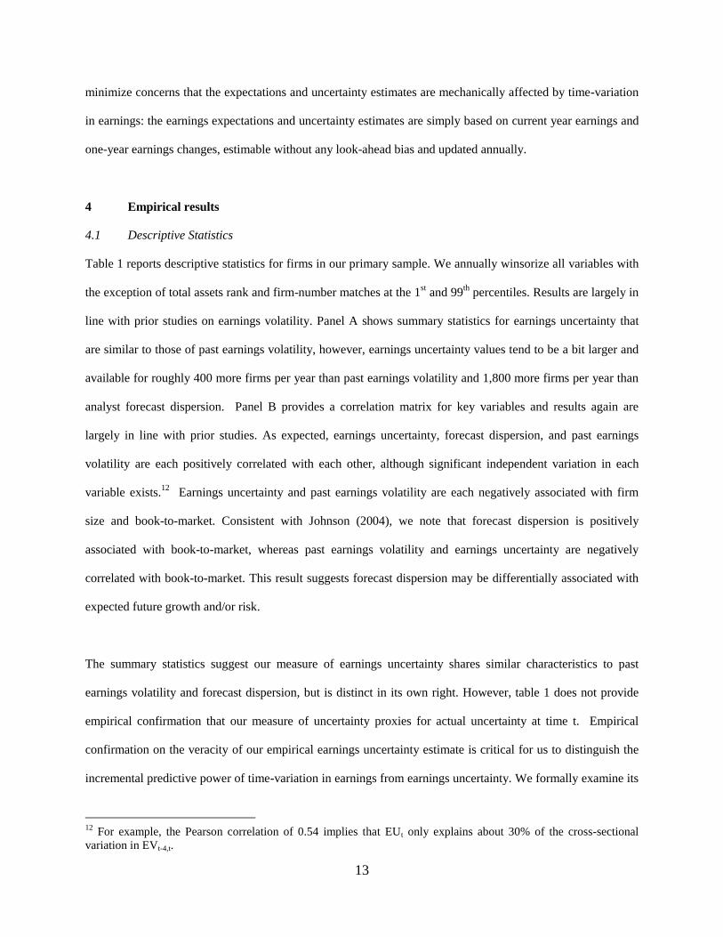
minimize concerns that the expectations and uncertainty estimates are mechanically affected by time-variation

in earnings: the earnings expectations and uncertainty estimates are simply based on current year earnings and

one-year earnings changes, estimable without any look-ahead bias and updated annually.

4 Empirical results

4.1 Descriptive Statistics

Table 1 reports descriptive statistics for firms in our primary sample. We annually winsorize all variables with

the exception of total assets rank and firm-number matches at the 1st and 99

th percentiles. Results are largely in

line with prior studies on earnings volatility. Panel A shows summary statistics for earnings uncertainty that

are similar to those of past earnings volatility, however, earnings uncertainty values tend to be a bit larger and

available for roughly 400 more firms per year than past earnings volatility and 1,800 more firms per year than

analyst forecast dispersion. Panel B provides a correlation matrix for key variables and results again are

largely in line with prior studies. As expected, earnings uncertainty, forecast dispersion, and past earnings

volatility are each positively correlated with each other, although significant independent variation in each

variable exists.12

Earnings uncertainty and past earnings volatility are each negatively associated with firm

size and book-to-market. Consistent with Johnson (2004), we note that forecast dispersion is positively

associated with book-to-market, whereas past earnings volatility and earnings uncertainty are negatively

correlated with book-to-market. This result suggests forecast dispersion may be differentially associated with

expected future growth and/or risk.

The summary statistics suggest our measure of earnings uncertainty shares similar characteristics to past

earnings volatility and forecast dispersion, but is distinct in its own right. However, table 1 does not provide

empirical confirmation that our measure of uncertainty proxies for actual uncertainty at time t. Empirical

confirmation on the veracity of our empirical earnings uncertainty estimate is critical for us to distinguish the

incremental predictive power of time-variation in earnings from earnings uncertainty. We formally examine its

12

For example, the Pearson correlation of 0.54 implies that EUt only explains about 30% of the cross-sectional

variation in EVt-4,t.

14

veracity in the next section.

4.2 Specification tests of cross-sectional earnings uncertainty

In this section, we empirically examine our matched-firm earnings uncertainty estimate against the more

common measures based on time-series earnings volatility and analyst forecast dispersion. Our specification

tests are presented in two formats. In our first set of tests (tables 2 and 3), we report results from a formal

regression analysis. The structure of the regression tests are based on well-known specification tests employed

in the finance literature for validating estimates of future return volatility and serve as a formal test of how well

our uncertainty variables proxy for actual uncertainty at time t, relative time-series based volatility measures.

The second set of specification tests are more descriptive in nature and illustrate how our uncertainty measures

vary across different industries, future accounting characteristics, and future market-based variables prior

studies associate with investor uncertainty.

4.2.1 Earnings uncertainty specification regressions

To assess how well the three uncertainty variables proxy for actual uncertainty at time t, we annually regress

the absolute value of unexpected t+1 earnings against their respective estimated volatilities at time t.

Specifically, table 2 reports the time-series average intercepts (γ0) and slopes (γ1) on our estimates of earnings

uncertainty (EU), earnings volatility (EV), and analyst forecast dispersion (Disp). The general intuition of

these regressions stems from the fact that the average absolute deviation from the expected value of a random

variable is roughly equivalent to the standard deviation of the random variable.13

In fact, a common proxy for

expected return volatility is the absolute value of returns over a given period (French, Schwert, Stambaugh

1987; Schwert 1990). If our matched-firm uncertainty estimates poorly proxy for uncertainty and, in the

extreme, are random noise, the intercept (γ0) will equal the sample mean of absolute value of unexpected

earnings and the slope (γ1) will equal 0.0. As our matched-firm volatility estimate more closely approximates

actual uncertainty at time t, (γ0) will decay to zero and (γ1) will increase to 1.0. Similar specification tests have

13

If the expected earnings model is unbiased, the square of unexpected earnings, UE2, equals σ

2Earn + ε where ε ~

N(0,1). Since (UE2)

1/2 = |UE|, the absolute value of unexpected earnings is a reasonable proxy for standard deviation

of expected earnings, EU.

15

been used to examine return volatility estimates (e.g., French, Schwert, Stambaugh 1987; Schwert 1989).14

Several empirical patterns from table 2 are worth noting. First, focusing on the All Stocks sample (shaded

across all three panels), the average intercepts (γ0) and slopes (γ1) in panel A suggest our matched-firm

earnings uncertainty measure is relatively well-specified. The average slopes on earnings uncertainty are 0.839

in the full sample and 0.952 in the latter-sample. Further, in the latter half of the sample (years 1991-2010), the

slope on earnings uncertainty is statistically indistinguishable from 1.0 with a much smaller standard error

(relative to the full sample), suggesting that our uncertainty measure performs better in the latter part of the

sample. Finally, the average intercepts on earnings uncertainty are small and statistically indistinguishable

from zero, suggesting that our earnings uncertainty measure is unbiased.

In contrast, the average slopes and intercepts on past earnings volatility (shaded rows in panel B) suggest that

past earnings volatility poorly proxies for earnings uncertainty. Focusing on the comparison of shaded rows

across panels A and B, the slopes (γ1) in panel B are significantly lower and the intercepts (γ0) are significantly

larger in absolute magnitude relative to those reported in in panel A. Further, the difference in slopes and

intercepts across panels A and B grows in the latter part of the full sample, suggesting that past earnings

volatility is becoming less similar to earnings uncertainty over time.

Interestingly, the slopes on forecast dispersion (panel C) suggest that forecast dispersion poorly proxies for

earnings uncertainty at time t.15

Again, focusing on the full sample (shaded rows in panel C), forecast

dispersion has an average predictive slope of 3.02 that is more than 8 standard errors away from 1.0. Perhaps

more disheartening is the positive and significant intercept (0.09; t-stat 3.28). This result suggests forecast

dispersion significantly understates earnings uncertainty. To the best of our knowledge, panel C offers the first

14

If one assumes earnings are a normally distributed random variable, the expected value of the absolute error is less

than the standard deviation from a normal distribution. In untabulated results, we assume earnings are normally

distributed and correct for this friction by multiplying all absolute errors by (2/π)-1/2

≈ 1.2533. Inferences are

qualitatively identical. 15

Since reliable forecast data does not exist over the full sample, we report specification test results for forecast

dispersion only in the latter sample. Results are qualitatively similar if we include forecast dispersion observations

beginning in 1976.

16

empirical evidence on the veracity of analyst forecast dispersion as a proxy for actual uncertainty at time t.

As an additional robustness check, the remaining, unshaded rows in table 2 show how well our earnings

uncertainty measure performs across select subsets of firms relative to past earnings volatility and forecast

dispersion. Firms are sorted annually into high or low quintiles based on book-to-market and change in

working capital. ‘Tiny’ firms are those with total assets below the 10th

NYSE-based total asset percentile.

Inferences are largely consistent to those reported in the shaded rows.

In sum, table 2 makes two important points. First, our matched-firm measure of earnings uncertainty is

reasonably well-specified on average and in select samples of firms experiencing extreme performance.

Second, forecast dispersion poorly proxies for earnings uncertainty. The forecast dispersion result is important

given the wide-spread belief in the accounting and finance literature suggesting forecast dispersion captures

future earnings uncertainty (Clement et al. 2003; Johnson 2004).

4.2.2 The predictive power of earnings volatility and earnings uncertainty for future earnings

Prior studies have shown that past earnings volatility has predictive power for future earnings (Minton et al.

2002; Dichev and Tang 2009). A subtle but important consideration in distinguishing the predictive power of

past earnings volatility from earnings uncertainty is to determine if our earnings uncertainty variable predicts

future earnings. Distinct from past earnings volatility, if our earnings uncertainty variable is well-specified, it

should not be associated with future earnings once expected earnings are controlled. Accordingly, we regress

future earnings on expected future earnings and earnings uncertainty. If our earnings uncertainty variable

captures actual future earnings uncertainty, and not an economic dynamic predictive of future performance, we

should find no relation between our earnings uncertainty variable and future earnings.

Similar to table 2, we provide results for the full time-series and the latter half of the time-series.16

As a

calibration exercise, in model 2 we regress future earnings on current earnings and past earnings volatility to

16

For brevity, we do not report results across the subsamples of firms experiencing extreme performance as reported

in table 2. Inferences are qualitatively identical in the subsamples to that reported in the full sample.

17

calibrate our results with those of Minton et al. (2002). Consistent with their results, we find a strong negative

relation between future earnings and past earnings volatility. This result suggests past earnings volatility is

informative of future profitability incremental to expected earnings. In model 1, we regress future earnings on

expected earnings and our earnings uncertainty variable. In contrast to the slope on past earnings volatility, the

slope on earnings uncertainty is significantly smaller (in absolute magnitude) and statistically indistinguishable

from zero. Finally, model 3 reports the predictive power of forecast dispersion for future earnings, controlling

for expected earnings (consensus EPS). Model 3 confirms analysts are optimistically biased (γ0 = -0.306; t-

statistic -12.23), although the bias does not lead to forecast dispersion having incremental predictive power for

future earnings to the consensus forecast.

In summary, the evidence reported in tables 2 and 3 suggests our earnings uncertainty variable is a reasonably

well-specified estimate of uncertainty in future earnings. Across the broad sample, the latter sample period,

and select subsamples of firms, we find specification slopes of approximately 1.0 and intercepts that are

approximately 0.0. Results also cast doubt on the veracity of forecast dispersion as a meaningful measure of

uncertainty, especially in firms experiencing extreme performance.

4.2.3 Descriptive Specification Analysis

As a final validation test, we provide descriptive relations of our earnings uncertainty measure across industry

classifications, future firm characteristics, and over time. Panel A of table 4 reports the relative proportion of

firm-year observations that fall into each earnings uncertainty quintile by industry. Obviously, there is no

‘right’ or ‘expected’ empirical relation between uncertainty quintiles and industry classification. However, ex-

ante, certain expectations exist with respect to specific industries. For example, the ‘Utility’ industry is often

characterized as an industry with very stable cash flows while the ‘Business Equipment’ industry, which is

comprised of many high technology, high R&D firms, is generally characterized as having unpredictable cash

flows. The empirical patterns noted in panel A generally comport to our expectations. Firms in the ‘Utility’,

‘Finance’ and ‘Energy’ industries tend to have lower earnings uncertainty, consistent in tenor to the idea that

firms in these industries have a relatively stable earnings process. In contrast, earnings uncertainty for firms in

18

the ‘Business Equipment’ industry is high. In fact, almost fifty percent of firms in this industry fall into the

fourth or fifth uncertainty quintile, percentages higher than any other industry.

In panel B, we report the time-series averages of three market-based characteristics and three accounting-based

characteristics prior studies have associated with investor uncertainty. Note, averages of the characteristics are

based on future realizations (i.e., t+1 realizations); thus, there should be no mechanical relation between our

uncertainty measures and the accounting realizations. Again, while we cannot definitively form expectations

of the expected differences across uncertainty quintiles for each characteristic, if our uncertainty variables

capture actual investor uncertainty at time t regarding t+1 realizations, we expect a monotonically increasing

pattern from low-to-high uncertainty quintiles. Indeed, this is the exact pattern panel B notes. Without

exception, there is a strong positive relation across earnings uncertainty quintiles for all six characteristics (all

differences, Q1-Q5, are significant, p-value ≤ 0.01).

Finally, in figures 1 and 2, each year we plot the median earnings uncertainty (Figure 1) and past earnings

volatility (Figure 2) for firms above and below the 10th NYSE total asset decile. Both figures reflect patterns

that are consistent in tenor to that reported in prior studies; Figure 1 notes an increase in earnings uncertainty

while Figure 2 notes a more modest increase in earnings volatility over time. Perhaps more interesting is the

fact that Figure 1 shows a much sharper increase in earnings uncertainty over the sample period up to 2000. In

2000, at the peak of the dotcom-fueled NASDAQ bull market, the median earnings uncertainty for small firms

topped out at around 12%, before sharply dropping in the subsequent years. In contrast, earnings volatility

increases more modestly over the sample period and continued to increase through 2005, a result driven by the

large negative earnings realizations realized in 2000 and 2001.

In sum, the evidence presented in tables 2, 3, and 4, along with that reflected in figures 1 and 2, suggests that

our earnings uncertainty variable is a reasonable proxy for actual earnings uncertainty at time t. Are our

estimates of earnings uncertainty perfect for each firm? Presumably not, but they appear to have empirical

properties that closely mirror the conceptual properties of actual earnings uncertainty. Further, because there is

19

minimal mechanical relation between our empirical estimates of earnings uncertainty, time-series earnings

volatility and analyst forecast dispersion variables, empirical tests that directly test the predictive power of the

different variables should offer useful insight as to the relative importance of earnings uncertainty and time-

series earnings variation.

V. Predictive power of earnings uncertainty

5.1 The relation between analyst forecast errors, past earnings volatility, and earnings uncertainty

Our first set of tests aims to distill the relative predictive power of earnings uncertainty from that of time-series

variation in earnings focuses on analyst forecast errors. Tension for this empirical investigation comes from

prior research suggesting that analysts do not understand the implications of past earnings volatility for future

earnings (Dichev and Tang 2009). Specifically, Dichev and Tang show that analysts fail to recognize that

earnings are less persistent for firms with high past earnings volatility. Unexplored by Dichev and Tang, but

important to the accounting literature, is determining whether the forecast bias is due to the time-series

variation in earnings or the underlying uncertainty surrounding future earnings. If our earnings uncertainty

variable subsumes the predictive power of past earnings volatility for forecast errors, it suggests that earnings

uncertainty, and not time-series variation in earnings, affects analyst forecasts.

To distill these two competing explanations from each other formally, we examine the predictive power of past

earnings volatility and earnings uncertainty for forecast errors across two specifications. In the first

specification (table 5, models 1-3), we regress analyst forecast errors on past earnings volatility, earnings

uncertainty, and some conventional control variables (prior period forecast error, size, book-to-market). If

time-series variation in earnings affects analyst forecasts, we should find a significantly negative association

between past earnings volatility and forecast errors. However, if the negative association found in prior studies

is due to the positive correlation between time-variation in earnings and earnings uncertainty, we should find a

strong negative slope on earnings uncertainty and an insignificant slope on past earnings volatility in model 3.

Analyst forecast errors are computed as the difference between the consensus analyst earnings forecast from

the summary unadjusted I/B/E/S file as of month 4 minus actual earnings. Thus, FEi,t+1 equals the consensus

20

earnings per share forecasts minus actual earnings per share (FEi,t+1=Et[EPSi,t+1]-EPSi,t+1). Consistent with prior

literature, we scale analyst earnings forecasts by market value of equity at the beginning of the period (fiscal

year end t) and begin our analysis of forecast errors in fiscal year 1977. Regression slopes are pooled and t-

statistics are clustered by firm (gvkey) and year (fyear).17

Empirical results are reported in table 5. In regressions 1 and 2, we find strong negative relations between

analyst forecast errors and earnings uncertainty (1) and past earnings volatility (2). The slopes are strong in

both specifications, but significantly larger for earnings uncertainty. In model 3, we directly test the

explanatory power of past earnings volatility and earnings uncertainty for analyst forecast errors. The purpose

of this test is to determine if the significant slope on past earnings volatility in model 1 is due to time-series

variation in earnings or earnings uncertainty. In model 3 we find a strong negative slope on earnings

uncertainty while past earnings volatility has very little incremental explanatory power.18

This result suggests

that earnings uncertainty is strongly predictive of future forecast errors (or that any predictive power of past

earnings volatility for forecast errors stems from its correlation with earnings uncertainty, not time-variation in

earnings).

In our second specification (table 5, models 4-6), we test the interactive effects of earnings uncertainty on how

efficiently analysts update their forecasts conditional on their most recent error. Building on the findings of

Dichev and Tang (2009), we are interested in determining whether earnings uncertainty or time-series variation

in earnings (as captured by past earnings volatility) is significantly associated with the autocorrelation structure

of forecast errors. If analysts fail to appreciate the persistence of earnings in firms with high earnings

uncertainty, we expect a negative interactive effect between the recent forecast error and earnings uncertainty.

However, if it is the time-series variation in earnings that explains the negative interaction noted by Dichev

and Tang, the interaction of past earnings volatility and the most recent forecast error should still explain

17

Qualitatively identical inferences result from Fama-MacBeth annual cross-sectional regressions with t-statistics

that are Newey-West adjusted. 18

The difference in slopes in model 3 on past earnings volatility (-0.018) and earnings uncertainty (-0.249) are

statistically different (p-value <0.01).

21

future forecast errors after controlling for earnings uncertainty.

The results from models 4-6 confirm the predictive power of earnings uncertainty. Consistent with the idea that

past earnings volatility is a weak proxy for earnings uncertainty, model 4 shows a much stronger predictive

main and interactive effect on earnings uncertainty relative to past earnings volatility in model 5. Further,

model 6 shows that the explanatory power of earnings uncertainty subsumes that of earnings uncertainty.

We interpret the results from table 5 as suggestive that time-series variation in earnings, as captured by past

earnings volatility, is not misinterpreted by analysts per se. Rather, past earnings volatility is correlated with

earnings uncertainty and it is earnings uncertainty, not time-series variation in earnings that leads to forecast

errors. This result is consistent with the notion that earnings uncertainty leads to systematic forecast biases.

However, as is well established in the accounting literature, analyst forecasts are subject to many biases and

the actions of analysts may not proxy for the actions of investors. Accordingly, in the next section we test

whether the actions of investors (as proxied by future return patterns) are associated with earnings uncertainty

in a direction and relative magnitude consistent with those of analysts.

5.2 The relation between future returns, past earnings volatility, and earnings uncertainty

To date, prior studies have failed to find that past earnings volatility or earnings uncertainty predict future

returns, especially over annual time periods (Zhang 2006; Frankel and Litov 2009; McInnis 2010).19

However,

as suggested above, this lack of a significant empirical relation could be due to the fact that empirical proxies

based on a time-series of earnings realizations jointly capture the effects of prior period economic shocks,

accrual estimation errors, and earnings uncertainty. Since each of these constructs is different, empirical

measures that jointly capture the constructs could mask the true predictive power of the individual constructs.

Prior studies examining the effect of information uncertainty predict, but do not explicitly show, that earnings

uncertainty should be negatively associated with future returns. For example, Jiang et al. (2005) define

19

One exception to this claim is Minton, Schrand, and Walther (2002) who find that fitted values from an earnings

prediction model that include past earnings volatility can be used to form a profitable trading strategy.

22

information uncertainty in terms of “value ambiguity, or the degree to which a firm’s value can be reasonably

estimated by even the most knowledgeable investors at reasonable costs.” Interestingly, Jiang et al. do not

examine direct measures of earnings uncertainty, choosing instead to proxy for information uncertainty using

indirect proxies such as firm age and implied equity duration. Zhang (2006) examines forecast dispersion

(among other proxies for uncertainty), but fails to find a significant relation between future returns and forecast

dispersion over an annual period.

The purpose of the subsequent tables is to examine the predictive power of earnings uncertainty for future

returns. The primary advantage of our earnings uncertainty variable compared to forecast dispersion (Zhang

2006) or firm characteristics thought to be correlated with earnings uncertainty (Zhang 2006; Jiang et al.

2005), is that our variable more precisely maps into the theoretical construct of earnings uncertainty. If we find

that our earnings uncertainty variable predicts future returns on an annual basis, it would be the first direct

empirical evidence that we are aware of showing long-horizon valuation consequences of earnings uncertainty.

To test if investor expectations are affected by earnings uncertainty directionally similar to analysts, we regress

future monthly returns against our earnings uncertainty measure and other firm characteristics known to be

associated with future returns using conventional Fama and Macbeth (1973) regressions in table 6. We report

empirical results for two sets of firms. Models 1-3 report the average regression slopes, t-statistics and sample

sizes from 504 monthly cross-sectional regressions, 1969:05–2011:04 for all firms with a share price greater

than $5 as of the last day of trading in the fourth month of year t+1. In models 4-6, we report regression results

for the sample of firms with estimates of either earnings uncertainty or forecast dispersion, 1984:05–2011:04.

The analysis reported in models 4-6 calibrate the economic and statistical significance of our earnings

uncertainty measure against the more commonly used forecast dispersion measure (Diether et al. 2002; Zhang

2006). All variables with the exception of future returns are winsorized monthly at the 1st and 99

th percentile.

All explanatory variables are updated once per fiscal year with the exception of return momentum, which is

updated monthly.

23

In general, inferences from the regression slopes reported in models 1-3 of table 6 are in line with the

contention that earnings uncertainty is positively associated with overly-optimistic future earnings

expectations. Slope coefficients on earnings uncertainty are strongly negative with slopes approximately 3.0

standard errors from zero across specifications 1 and 2. In specification 3, we substitute the coefficient of

variation for earnings uncertainty. The coefficient of variation scales earnings uncertainty by the absolute value

of expected earnings, thereby preventing firms with extreme earnings (and generally higher earnings volatility)

from disproportionately populating the extremes of the earnings uncertainty distribution.20

Inferences with

respect to coefficient of variation are consistent to those reported in model 1, albeit significantly stronger with

a negative slope on the scaled earnings uncertainty variable that is more than 4.5 standard errors from zero.

In models 4-6, we directly compare the predictive power of our measure of earnings uncertainty against that

derived from forecast dispersion. Diether et al. (2002) show that forecast dispersion scaled by the absolute

value of expected earnings is negatively associated with future returns. While Diether et al. suggest that their

forecast dispersion measure captures opinion divergence across investors, others have interpreted forecast

dispersion as capturing earnings uncertainty (Johnson 2004; Zhang 2006). Accordingly, models 4-6 provide a

direct test of the incremental predictive power of our earnings uncertainty measure against one derived from

forecast dispersion.

Results show that our earnings uncertainty measure largely subsumes the predictive power of forecast

dispersion for future returns. Perhaps surprising to some, our results show that forecast dispersion is a weak

predictor of future returns over an annual period. In fact, however, these results agree with those in Diether et

al. and Zhang (2006).21

These results also agree with our fundamental premise that better estimates of the first

moment (future earnings) produce better estimates of the second moment of earnings (future earnings

uncertainty), which lead to more precise inferences on the predictive power of earnings uncertainty.

20

Minton and Schrand (1999), Minton, Schrand, and Walther (2002), and Diether et al. (2002) each measure

volatility using this form of the coefficient of variation. 21

Diether et al. report similar results in their lagged forecast analysis (Figure 1; pp. 2131). Note hedge returns are

statistically indistinguishable from zero at approximately four months. Zhang (2006) also finds insignificant hedge

returns when forecast dispersion is used to proxy for uncertainty and only updated once a year (table 2; pp. 114).

24

5.3 The relation between contemporaneous returns and change in earnings uncertainty

To further explore the valuation consequences of earnings uncertainty, we examine the relation between the

one-year change in earnings uncertainty and one-year equity returns. The purpose of these tests is to examine

the other side of the earnings uncertainty relation with equity returns. That is, if high earnings uncertainty is

negatively associated with future returns due to overly-optimistic earnings expectations, then changes in

earnings uncertainty should be positively associated with contemporaneous period returns. We test this

formally across two distinct specifications in table 7.

In models 1-3 of table 7 we annually regress annual buy-and-hold returns (t-1, t) on the contemporaneous one-

year change in earnings uncertainty, lagged uncertainty, and a series of conventional control variables

associated with realized and expected performance. Consistent with prior literature, we expect positive slopes

on one-year earnings change, lagged earnings, book-to-market, and a negative slope on size. If earnings

uncertainty is positively associated with the forecast optimism of investors, then we expect positive slopes on

one-year change in earnings uncertainty and lagged earnings uncertainty.

Average slopes on the control variables are in line with expectations. Model 1 notes positive slopes on

earnings change, lagged earnings, and book-to-market and a negative slope on lagged size. Consistent with

earnings uncertainty affecting investor expectations, models 2 and 3 note positive slopes on the one year

change in earnings uncertainty in both specifications (2,3) and on lagged earnings uncertainty in (3).

In models 4-6, we examine the predictive power of change in earnings uncertainty on the so-called intangible

returns. Introduced by Daniel and Titman (2006), intangible returns are interpreted as the component of

realized returns that is unrelated (orthogonal) to contemporaneous realized accounting performance. If earnings

uncertainty explains equity returns because it affects investors’ expectations of future earnings, and not due to

its relation with realized accounting performance, then a predictive relation between intangible returns by

change in earnings uncertainty will offer powerful corroborative evidence to that noted in models 1-3.

25

For simplicity, we define intangible returns as the logarithmic change in market to book between t-1 and t (see

Fama and French 2008).22

Explanatory variables remain the same as models 1-3. Similar to models 1-3, we

expect a positive relation between intangible return and book-to-market and a negative relation with firm size

as these variables jointly capture variation in earnings expectations and firm risk. Importantly, we expect an

insignificant relation between intangible returns and earnings since intangible returns are unrelated to

accounting-based performance. Finally, to the extent that earnings uncertainty is positively associated with

investor expectations of future earnings, we expect a positive relation between intangible returns and the

change in earnings uncertainty.

Results in models 4-6 are line with our expectations. These relations suggest that as the uncertainty about a

firm’s future earnings process increases, ceteris paribus, a firm’s market-to-book ratio will tend to increase for

reasons unrelated to expected growth, risk, or realized earnings.

6 Robustness Tests

6.1 Portfolio returns

Table 8 examines the relation between future monthly returns and earnings uncertainty from a portfolio

perspective. Because earnings uncertainty and forecast dispersion are strongly associated with size and book-

to-market, and these characteristics also predict returns, our portfolios are formed based on the component of

earnings uncertainty that is orthogonal to our control variables. That is, each month we regress earnings

uncertainty or the coefficient of variation on our control variables (size, B/M, momentum, and accruals) and

form portfolios based on the residuals from this regression. This design choice allows us isolate the component

of uncertainty unrelated to the control variables and calibrate its nonparametric relation to future returns.

Consistent with prior empirical tables, we report results for earnings uncertainty over the full 504 month

sample (1969:05–2011:04) and the 324 month later sample for forecast dispersion (1984:05-2011:04). The

22

Fama and French (2008, p. 2985, equation 7) propose a simpler empirical design to measure intangible returns

than Daniel and Titman (2006). Specifically, intangible return = log(BMt-1) – log(BMt)

26

empirical relations noted in table 8 agree with those of table 6. Average monthly hedge returns over the full

sample are 0.21 and 0.33 per month for portfolios (1) and (2), each significantly different than zero. Over the

later sample, we find similar, albeit slightly weaker results. We investigate the cause of this drop in predictive

power in the next section.

6.2 Time-series analysis

Accounting and finance researchers tend to focus on the sign and statistical significance from a time-series

average of cross-sectional regressions to confirm whether a firm characteristic is associated with future returns.

Since Fama-Macbeth slopes and t-statistics are functions of equal-weighted averages computed over the

sample period, they are sensitive to extreme realizations. Further, as conventionally reported, the FM slopes

and t-statistics tell us very little about whether a relation is getting stronger or weaker over the time period.

Accordingly, it is possible that the negative relation between future returns and earnings uncertainty is a relic

of a very strong early-period relation and does not reflect more recent period dynamics.

As a final robustness test on the predictive relation of earnings uncertainty and future returns, we plot the

time-series variation in the 10-year rolling average FM slopes on explanatory variables in Figure 3. The

primary purpose of this analysis is to examine whether the average slopes on earnings uncertainty change over

time or are sensitive to certain subperiods of the full sample.

Figure 3 reports plots of the 10-year rolling average of the monthly slopes from model 1 of table 6. We exclude

size and B/M from the plot because their slope magnitudes are very different and the time-series variation in

the slopes of the other control variables is not the primary interest of this study (however, these variables are

still used as explanatory variables). Since our future return series begins in 1969:05, the time-series plots span

1979:04 to 2011:04.

Figure 3 shows that the slopes on accruals and momentum tend to shrink over time, but their 10 year rolling

average tend to lie completely below or above the x-axis. The decline in slopes on momentum and accruals

27

suggest that past estimates on these characteristics tend to overestimate the current predictive significance of

these variables and are consistent with prior studies (Green, Hand, Soliman 2011; Lewellen 2013).

In contrast to the slopes on the control variables, there is no apparent decline in the rolling slope average on

earnings uncertainty (although the slopes are more volatile). We do, however, note a severe positive spike on

the earnings uncertainty slopes in late 1999, early 2000. A similar result is noted in Diether et al. where they

note the behavior of high dispersion stock strongly reverse in 2000 from the predictive patterns of years 1983-

1999 (pp. 2127). In untabulated analysis, we find that this spike is concentrated in microcap NASDAQ firms

between 1999:11 – 2000:02. In particular, there were an above average number of high uncertainty firms

realizing monthly returns well in excess of 200% in this four month period.

6.3 Alternative Specification Discussion

Our research design groups firms based on summary characteristics prior studies have found to have strong

relations with earnings predictability. The simplicity of the matching process we employ to derive our measure

of earnings uncertainty could elicit an almost endless list of alternative matching criteria. However, while

matching firms on increasingly more precise firm characteristics may produce more precise earnings

expectations, it will also tend to exclude many more firms. The more firms excluded from the primary sample

of firms, the higher the likelihood our inferences could be biased (by the exclusion of firms), thereby

decreasing the generalizability of our results to a broad cross-section of firms. Without explicitly reporting the

details, we can report our empirical results are robust to alternative matching criteria based on earnings and

firm size. Specifically, varying the definition of ‘comparable’ earnings performance by reasonable amounts

has little effect on our empirical results.

In addition, some readers have questioned whether the predictive qualities of earnings uncertainty are

associated with the cash flow or accrual component of earnings. Without reporting the details, we estimate

cash flow uncertainty using the same empirical design as described for earnings in section 3.1, where cash flow

equals earnings before extraordinary items, plus non-cash reconciling items from the statement of cash flow,

28

minus change in net working capital. We find that cash flow uncertainty is strongly negatively associated with

future returns; however the predictive power of earnings uncertainty is stronger than cash flow uncertainty

suggesting that both the cash flow and accrual component of earnings uncertainty have predictive power.

7 Conclusion

This study examines the predictive power of past earnings volatility. We hypothesize that past earnings

volatility jointly captures two distinct economic dynamics: time-series variation in earnings and earnings

uncertainty. Due to the tight connection between the two dynamics, prior empirical studies have been unable to

distill the predictive power of earnings uncertainty from that associated with time-series variation in earnings.

We develop a new measure of future earnings uncertainty based on a matched-firm empirical design. We show

that our earnings uncertainty variable is a well specified estimate of actual uncertainty and dominates those

based on time-variation in earnings realizations and analyst forecast dispersion. Collectively, our empirical

results strongly and consistently suggest that earnings uncertainty, and not time-series variation in earnings,

leads to overly-optimistic future earnings forecasts of equity analysts and investors.

Our results contribute along several dimensions of accounting research. First, we show that earnings

uncertainty has a strong (negative) predictive relation for analyst forecast errors and future returns. Prior

studies examining information uncertainty have hypothesized, but have not empirically documented, that

earnings uncertainty should be associated with overly-optimistic forecasts. An obvious alternative explanation

for this ‘no-result’ finding from prior studies is that earnings uncertainty does not affect firm valuation,

consistent with the existence of influential market agents arbitraging away pricing inefficiencies (Diamond and

Verrecchia 1987). Our study is the first to show that uncertainty in future earnings is value-relevant and that

this relevance comes from its relation with future earnings expectations. Further, in contrast to Diether et al.

(2002) and Ang et al. (2006) who show relatively short horizon predictive power for future returns, our

evidence suggests a more persistent negative relation that holds for at least one year.

Second, we build from the work of Blouin, Core, and Guay (2010) and offer firm-specific proxy for future

29

earnings uncertainty. Blouin et al. note that the level of taxable earnings does not follow a random-walk, which

can lead to questionable inferences on the value of the debt-tax shield when past earnings volatility is used as a

proxy for future earnings uncertainty. We extend their empirical model to profitability and propose a firm-

specific (rather than portfolio-level) measure of earnings uncertainty. While our matched-firm earnings

uncertainty variable is presumably imperfect, specification tests suggest it is a much better proxy for earnings

uncertainty than past earnings volatility or forecast dispersion.

Finally, we believe our study has implications for future research along several dimensions. Time-series

variation in earnings has been used to explain variation in investment policies (Minton and Schrand 1999),

firm valuation (Rountree et al. 2008), and earnings quality (Dechow and Dichev 2002; Leuz et al. 2003). As

noted above, time-series variation in earnings is positively correlated with future earnings uncertainty, but the

connection is not perfect and cross-sectional variation in the predictive power of these two constructs probably

exists across different firm types. Future research could examine differences in the predictive power of

earnings uncertainty and time-series variation in earnings in these settings.

30

References

Ang, A., R. Hodrick, Y. Xing and X. Zhang. 2006. The cross-section of volatility and expected returns. Journal

of Finance 61: 259–299.

Baker, M., J. Wurgler, 2011. Benchmarks as Limits to Arbitrage: Understanding the Low-Volatility

Anomaly. Financial Analysts Journal, 67 (1).

Ball, R., & Watts, R. 1972. Some time series properties of accounting income. The Journal of Finance, 27(3),

663-681.

Barber, B.M. and J.D. Lyon. 1996. Detecting abnormal operating performance: The empirical power and

specification of test statistics. Journal of Financial Economics 41: 359-399.

Barron, O.E., O. Kim, S.C. Lim and D.E. Stevens. 1998. Using analysts’ forecasts to measure properties of

analysts’ information environment. The Accounting Review 73: 421–433.

Beaver, W. H. 1970. The time series behavior of earnings. Journal of Accounting Research, 62-99.

Beaver, W., P. Kettler and M. Scholes. 1970. The association between market determined and accounting

determined risk measures. The Accounting Review 45: 654-682.

Blouin, J.L, J. Core and W. Guay. 2010. Have the Benefits of Debt Been Overstated? Journal of Financial

Economics 98: 195-213.

Brown, L. and S. Laroque. 2013. I/B/E/S Reported Actual EPS and Analysts’ Inferred Actual EPS. The

Accounting Review 88(3): 853-880.

Clement, M., R. Frankel and J. Miller. 2003. Confirming management earnings forecasts, earnings uncertainty,

and stock returns. Journal of Accounting Research 41: 653–679.

Daniel, K., D. Hirshleifer, A. Subrahmanyam, 1998. Investor psychology and security market under‐and

overreactions. Journal of Finance 53 (6), 1839-1885.

Daniel, K. and S. Titman. 2006. Market reactions to tangible and intangible information. Journal of Finance

61: 1605-1643.

Dehow, P.M., and I.D. Dichev. 2002. The quality of accruals and earnings: The role of accrual estimation

errors. The Accounting Review 77: 35-59.

Dechow, P., W. Ge and C. Schrand. 2010. Understanding earnings quality: A review of the proxies, their

determinants and their consequences. Journal of Accounting and Economics 50: 344-401.

Diamond, D.W. and R.E. Verrecchia. 1987. Constraints on short-selling and asset price adjustment to private

information. Journal of Financial Economics 18: 277-311.

Dichev, I.D. and V.W. Tang. 2009. Earnings Volatility and Earnings Predictability. Journal of Accounting and

Economics 47: 160-181.

Diether, K., C. Malloy and A. Scherbina. 2002. Difference of opinion and the cross section of stock returns.

The Journal of Finance 57: 2113-41.

Easley, D., and M. O’Hara. 2004. Information and the cost of capital. Journal of Finance 59: 1553-1583.

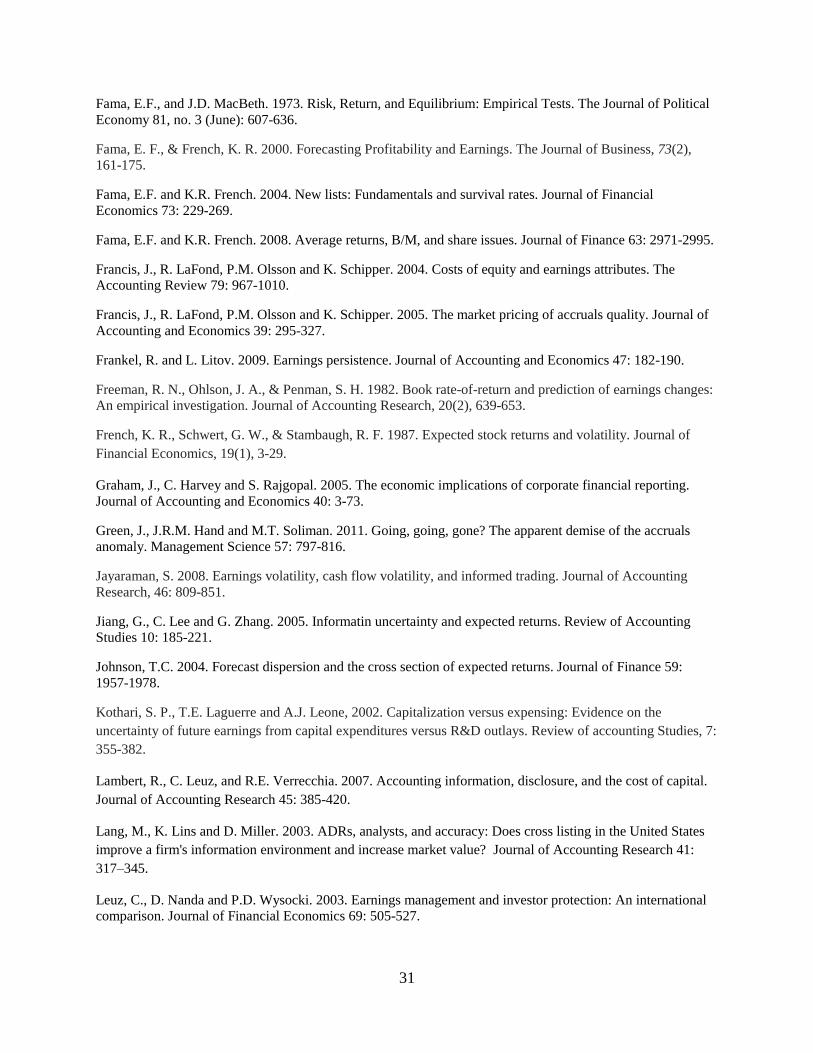
31

Fama, E.F., and J.D. MacBeth. 1973. Risk, Return, and Equilibrium: Empirical Tests. The Journal of Political

Economy 81, no. 3 (June): 607-636.

Fama, E. F., & French, K. R. 2000. Forecasting Profitability and Earnings. The Journal of Business, 73(2),

161-175.

Fama, E.F. and K.R. French. 2004. New lists: Fundamentals and survival rates. Journal of Financial

Economics 73: 229-269.

Fama, E.F. and K.R. French. 2008. Average returns, B/M, and share issues. Journal of Finance 63: 2971-2995.

Francis, J., R. LaFond, P.M. Olsson and K. Schipper. 2004. Costs of equity and earnings attributes. The

Accounting Review 79: 967-1010.

Francis, J., R. LaFond, P.M. Olsson and K. Schipper. 2005. The market pricing of accruals quality. Journal of

Accounting and Economics 39: 295-327.

Frankel, R. and L. Litov. 2009. Earnings persistence. Journal of Accounting and Economics 47: 182-190.

Freeman, R. N., Ohlson, J. A., & Penman, S. H. 1982. Book rate-of-return and prediction of earnings changes:

An empirical investigation. Journal of Accounting Research, 20(2), 639-653.

French, K. R., Schwert, G. W., & Stambaugh, R. F. 1987. Expected stock returns and volatility. Journal of

Financial Economics, 19(1), 3-29.

Graham, J., C. Harvey and S. Rajgopal. 2005. The economic implications of corporate financial reporting.

Journal of Accounting and Economics 40: 3-73.

Green, J., J.R.M. Hand and M.T. Soliman. 2011. Going, going, gone? The apparent demise of the accruals

anomaly. Management Science 57: 797-816.

Jayaraman, S. 2008. Earnings volatility, cash flow volatility, and informed trading. Journal of Accounting

Research, 46: 809-851.

Jiang, G., C. Lee and G. Zhang. 2005. Informatin uncertainty and expected returns. Review of Accounting

Studies 10: 185-221.

Johnson, T.C. 2004. Forecast dispersion and the cross section of expected returns. Journal of Finance 59:

1957-1978.

Kothari, S. P., T.E. Laguerre and A.J. Leone, 2002. Capitalization versus expensing: Evidence on the

uncertainty of future earnings from capital expenditures versus R&D outlays. Review of accounting Studies, 7:

355-382.

Lambert, R., C. Leuz, and R.E. Verrecchia. 2007. Accounting information, disclosure, and the cost of capital.

Journal of Accounting Research 45: 385-420.

Lang, M., K. Lins and D. Miller. 2003. ADRs, analysts, and accuracy: Does cross listing in the United States

improve a firm's information environment and increase market value? Journal of Accounting Research 41:

317–345.

Leuz, C., D. Nanda and P.D. Wysocki. 2003. Earnings management and investor protection: An international comparison. Journal of Financial Economics 69: 505-527.

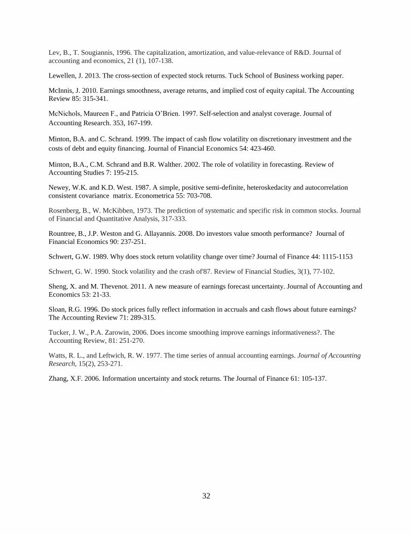
32

Lev, B., T. Sougiannis, 1996. The capitalization, amortization, and value-relevance of R&D. Journal of

accounting and economics, 21 (1), 107-138.

Lewellen, J. 2013. The cross-section of expected stock returns. Tuck School of Business working paper.

McInnis, J. 2010. Earnings smoothness, average returns, and implied cost of equity capital. The Accounting

Review 85: 315-341.

McNichols, Maureen F., and Patricia O’Brien. 1997. Self-selection and analyst coverage. Journal of

Accounting Research. 353, 167-199.

Minton, B.A. and C. Schrand. 1999. The impact of cash flow volatility on discretionary investment and the

costs of debt and equity financing. Journal of Financial Economics 54: 423-460.

Minton, B.A., C.M. Schrand and B.R. Walther. 2002. The role of volatility in forecasting. Review of

Accounting Studies 7: 195-215.

Newey, W.K. and K.D. West. 1987. A simple, positive semi-definite, heteroskedacity and autocorrelation

consistent covariance matrix. Econometrica 55: 703-708.

Rosenberg, B., W. McKibben, 1973. The prediction of systematic and specific risk in common stocks. Journal

of Financial and Quantitative Analysis, 317-333.

Rountree, B., J.P. Weston and G. Allayannis. 2008. Do investors value smooth performance? Journal of

Financial Economics 90: 237-251.

Schwert, G.W. 1989. Why does stock return volatility change over time? Journal of Finance 44: 1115-1153

Schwert, G. W. 1990. Stock volatility and the crash of'87. Review of Financial Studies, 3(1), 77-102.

Sheng, X. and M. Thevenot. 2011. A new measure of earnings forecast uncertainty. Journal of Accounting and

Economics 53: 21-33.

Sloan, R.G. 1996. Do stock prices fully reflect information in accruals and cash flows about future earnings?

The Accounting Review 71: 289-315.

Tucker, J. W., P.A. Zarowin, 2006. Does income smoothing improve earnings informativeness?. The

Accounting Review, 81: 251-270.

Watts, R. L., and Leftwich, R. W. 1977. The time series of annual accounting earnings. Journal of Accounting

Research, 15(2), 253-271.

Zhang, X.F. 2006. Information uncertainty and stock returns. The Journal of Finance 61: 105-137.

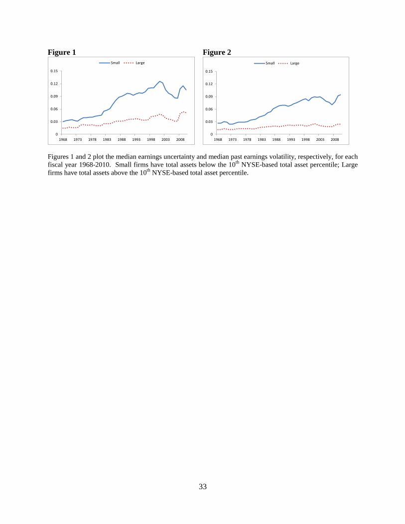
33

Figure 1 Figure 2

0

0.03

0.06

0.09

0.12

0.15

1968 1973 1978 1983 1988 1993 1998 2003 2008

Small Large

0

0.03

0.06

0.09

0.12

0.15

1968 1973 1978 1983 1988 1993 1998 2003 2008

Small Large

Figures 1 and 2 plot the median earnings uncertainty and median past earnings volatility, respectively, for each

fiscal year 1968-2010. Small firms have total assets below the 10th NYSE-based total asset percentile; Large

firms have total assets above the 10th NYSE-based total asset percentile.

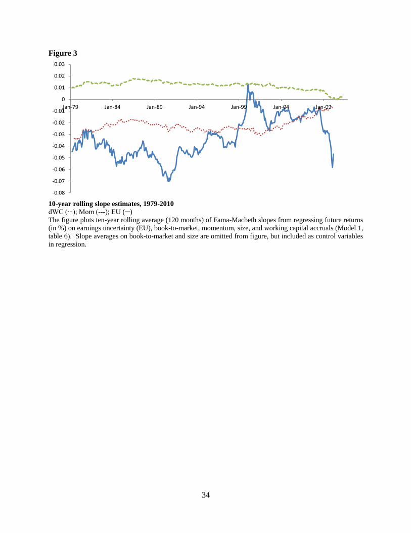
34

Figure 3

-0.08

-0.07

-0.06

-0.05

-0.04

-0.03

-0.02

-0.01

0

0.01

0.02

0.03

Jan-79 Jan-84 Jan-89 Jan-94 Jan-99 Jan-04 Jan-09

10-year rolling slope estimates, 1979-2010

dWC (∙∙∙); Mom (---); EU (─)

The figure plots ten-year rolling average (120 months) of Fama-Macbeth slopes from regressing future returns

(in %) on earnings uncertainty (EU), book-to-market, momentum, size, and working capital accruals (Model 1,

table 6). Slope averages on book-to-market and size are omitted from figure, but included as control variables

in regression.

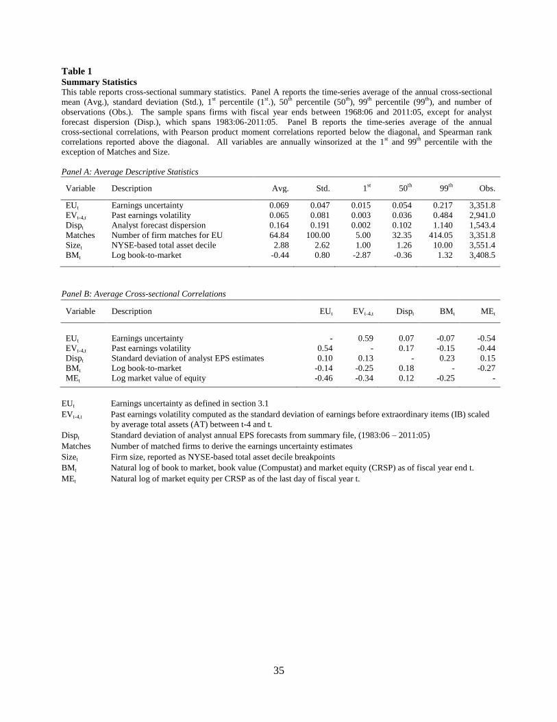
35

Table 1 Summary Statistics This table reports cross-sectional summary statistics. Panel A reports the time-series average of the annual cross-sectional

mean (Avg.), standard deviation (Std.), 1st percentile (1

st.), 50

th percentile (50

th), 99

th percentile (99

th), and number of

observations (Obs.). The sample spans firms with fiscal year ends between 1968:06 and 2011:05, except for analyst

forecast dispersion (Disp.), which spans 1983:06-2011:05. Panel B reports the time-series average of the annual

cross-sectional correlations, with Pearson product moment correlations reported below the diagonal, and Spearman rank

correlations reported above the diagonal. All variables are annually winsorized at the 1st and 99

th percentile with the

exception of Matches and Size.

Panel A: Average Descriptive Statistics

Variable Description Avg. Std. 1

st 50

th 99

th Obs.

EUt Earnings uncertainty 0.069 0.047 0.015 0.054 0.217 3,351.8

EVt-4,t Past earnings volatility 0.065 0.081 0.003 0.036 0.484 2,941.0

Dispt Analyst forecast dispersion 0.164 0.191 0.002 0.102 1.140 1,543.4

Matches Number of firm matches for EU 64.84 100.00 5.00 32.35 414.05 3,351.8

Sizet NYSE-based total asset decile 2.88 2.62 1.00 1.26 10.00 3,551.4

BMt Log book-to-market -0.44 0.80 -2.87 -0.36 1.32 3,408.5

Panel B: Average Cross-sectional Correlations

Variable Description EUt EVt-4,t Dispt BMt MEt

EUt Earnings uncertainty - 0.59 0.07 -0.07 -0.54

EVt-4,t Past earnings volatility 0.54 - 0.17 -0.15 -0.44

Dispt Standard deviation of analyst EPS estimates 0.10 0.13 - 0.23 0.15

BMt Log book-to-market -0.14 -0.25 0.18 - -0.27

MEt Log market value of equity -0.46 -0.34 0.12 -0.25 -

EUt Earnings uncertainty as defined in section 3.1

EVt-4,t Past earnings volatility computed as the standard deviation of earnings before extraordinary items (IB) scaled

by average total assets (AT) between t-4 and t.

Dispt Standard deviation of analyst annual EPS forecasts from summary file, (1983:06 – 2011:05)

Matches Number of matched firms to derive the earnings uncertainty estimates

Sizet Firm size, reported as NYSE-based total asset decile breakpoints

BMt Natural log of book to market, book value (Compustat) and market equity (CRSP) as of fiscal year end t.

MEt Natural log of market equity per CRSP as of the last day of fiscal year t.

36

Table 2 Annual cross-sectional specification regressions: 1968-2010 This table reports the time-series average intercepts and slopes from the following annual cross-sectional regressions:

Panel A: Panel B: Panel C:

Real_Vol = γ0 + γ1 EU + e Real_Vol = γ0 + γ1 EV + e Real_Vol = γ0 + γ1 Disp + e

Earnt+1 = β0 + β1 Et[Earnt+1] + e Earnt+1 = β0 + β1 Earnt + e EPSt+1 = β0 + β1+AFt + e

Real_Vol is defined in each panel as the absolute value of unexpected earnings. In panel A, unexpected earnings is the

difference between realized earnings and expected earnings from the matched-firm expectation model; in panel B,

unexpected earnings is the difference between realized earnings and current earnings; in panel C, unexpected earnings is

the difference between the consensus analyst EPS estimate and realized EPS, per the unadjusted I/B/E/S summary file

(month 4 of fiscal year t+1). Analyst forecasts and EPS realizations are adjusted to account for stock splits occurring

between forecast date and announcement date. Since analyst forecast data is not available until 1976, we only report

results for the 1991-2010 sample. All independent variables are winsorized at the 1st and 99

th percentile. To minimize the

look-ahead bias, future earnings values used in panels A and B are winsorized between -1.0 and 1.0. In panel C, we trim

unexpected EPS realizations greater than 50% of market equity ( ~ 1% of sample). All other variables defined in table 1.

Full Sample 1968-2010 Late Sample 1991-2010

Sample FM slopes γ0 γ1 β0 β1 Obs. γ0 γ1 β0 β1 Obs.

Panel A: Earnings Uncertainty

All Avg. 0.000 0.839 -0.005 0.967 3340 -0.004 0.952 -0.006 0.945 3848 stocks FM t-stat (0.11) (14.87) (-2.28) (60.15) (-1.82) (29.86) (-1.72) (91.03) Low Avg. 0.001 0.883 -0.003 0.938 636 -0.005 1.010 -0.002 0.873 748 dWCt. FM t-stat (0.49) (13.34) (-0.99) (27.13) (-1.74) (25.80) (-0.37) (52.31) High Avg. 0.008 0.827 -0.017 0.960 656 0.003 0.984 -0.018 0.936 756 dWCt FM t-stat (3.70) (10.95) (-4.08) (48.29) (1.44) (35.76) (-3.24) (67.49) Low Avg. 0.007 0.912 -0.004 1.000 617 0.003 1.035 0.003 0.967 705 BM FM t-stat (3.36) (15.79) (-0.71) (36.54) (1.12) (33.45) (0.38) (57.47) High Avg. 0.008 0.670 -0.013 0.871 668 0.006 0.796 -0.020 0.822 784 BM FM t-stat (2.59) (10.62) (-3.38) (29.24) (1.02) (19.35) (-3.80) (41.46) Tiny Avg. 0.004 0.817 -0.009 0.960 1814 -0.001 0.957 -0.011 0.934 2130 FM t-stat (1.71) (11.74) (3.00) (47.88) (-0.22) (29.03) (-2.71) (83.52)

Panel B: Past Earnings Volatility

All Avg. 0.025 0.606 -0.005 0.781 2930 0.039 0.505 -0.010 0.757 3348

stocks FM t-stat (4.62) (12.65) (-1.58) (42.16) (10.44) (9.33) (-4.18) (77.90)

Low Avg. 0.034 0.702 -0.001 0.730 576 0.056 0.558 -0.006 0.697 667 dWCt FM t-stat (4.18) (10.31) (-0.13) (28.54) (16.19) (9.41) (-1.44) (49.07) High Avg. 0.036 0.491 -0.021 0.802 524 0.053 0.429 -0.029 0.767 612 dWCt FM t-stat (5.59) (14.93) (-4.51) (42.91) (14.21) (9.67) (-7.33) (75.85) Low Avg. 0.045 0.552 -0.003 0.801 534 0.072 0.417 -0.006 0.784 634 BM FM t-stat (4.45) (9.91) (-0.75) (39.85) (22.43) (8.52) (-0.94) (61.63) High Avg. 0.024 0.674 -0.014 0.690 609 0.036 0.606 -0.025 0.618 699 BM FM t-stat (4.58) (14.47) (-2.69) (20.04) (5.46) (8.74) (-4.66) (28.04) Tiny Avg. 0.039 0.556 -0.013 0.770 1465 0.061 0.443 -0.024 0.751 1742 FM t-stat (4.74) (11.03) (-2.76) (38.14) (13.17) (8.83) (-7.65) (76.70) Panel C: Forecast Dispersion

All Avg. 0.094 3.022 -0.318 1.162 2255

stocks FM t-stat (3.28) (12.98) (-10.73) (90.88)

Low Avg. 0.129 2.333 -0.235 1.133 335 dWCt FM t-stat (2.99) (6.63) (-5.53) (28.86) High Avg. 0.101 3.962 -0.365 1.173 417 dWCt FM t-stat (1.05) (3.43) (-11.05) (17.31) Low Avg. 0.001 4.137 -0.304 1.255 440 BM FM t-stat (0.02) (5.73) (-6.38) (30.62) High Avg. 0.199 2.177 -0.385 1.129 281 BM FM t-stat (5.39) (6.09) (-10.05) (36.66) Tiny Avg. 0.224 1.074 -0.165 1.012 767 FM t-stat (10.96) (27.42) (-4.86) (156.86)

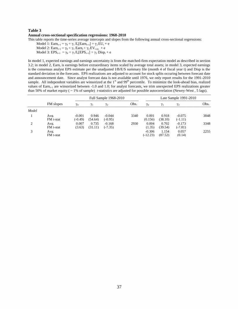
37

Table 3 Annual cross-sectional specification regressions: 1968-2010 This table reports the time-series average intercepts and slopes from the following annual cross-sectional regressions:

Model 1: Earnt+1 = γ0 + γ1 Et[Earnt+1] + γ2 EUt + e

Model 2: Earnt+1 = γ0 + γ1 Earnt + γ2 EVt-4,t + e

Model 3: EPSt+1 = γ0 + γ1 Et[EPSt+1] + γ2 Dispt + e

In model 1, expected earnings and earnings uncertainty is from the matched-firm expectation model as described in section

3.2; in model 2, Earnt is earnings before extraordinary items scaled by average total assets; in model 3, expected earnings

is the consensus analyst EPS estimate per the unadjusted I/B/E/S summary file (month 4 of fiscal year t) and Disp is the

standard deviation in the forecasts. EPS realizations are adjusted to account for stock splits occuring between forecast date

and announcement date. Since analyst forecast data is not available until 1976, we only report results for the 1991-2010

sample. All independent variables are winsorized at the 1st and 99

th percentile. To minimize the look-ahead bias, realized

values of Earnt+1 are winsorized between -1.0 and 1.0; for analyst forecasts, we trim unexpected EPS realizations greater

than 50% of market equity ( ~ 1% of sample) t-statistics are adjusted for possible autocorrelation (Newey-West , 5 lags).

Full Sample 1968-2010 Late Sample 1991-2010

FM slopes γ0 γ1 γ2 Obs. γ0 γ1 γ2 Obs.

Model

1 Avg. -0.001 0.946 -0.044 3340 0.001 0.918 -0.075 3848 FM t-stat (-0.49) (54.64) (-0.95) (0.156) (38.10) (-1.11) 2 Avg. 0.007 0.735 -0.168 2930 0.004 0.702 -0.173 3348 FM t-stat (3.63) (31.11) (-7.35) (1.35) (39.54) (-7.81) 3 Avg. -0.306 1.154 0.057 2255 FM t-stat (-12.23) (87.52) (0.14)

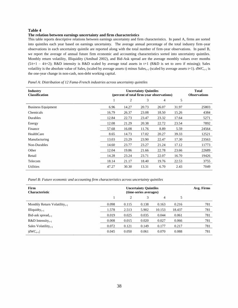
38

Table 4 The relation between earnings uncertainty and firm characteristics This table reports descriptive relations between earnings uncertainty and firm characteristics. In panel A, firms are sorted

into quintiles each year based on earnings uncertainty. The average annual percentage of the total industry firm-year

observations in each uncertainty quintile are reported along with the total number of firm-year observations. In panel B,

we report the average of annual future firm economic and accounting characteristics sorted into uncertainty quintiles.

Monthly return volatility, Illiquidity (Amihud 2002), and Bid-Ask spread are the average monthly values over months

(5/t+1 – 4/t+2); R&D intensity is R&D scaled by average total assets in t+1 (R&D is set to zero if missing); Sales

volatility is the absolute value of Salest (scaled by average assets t) minus Salest+1 (scaled by average assets t+1). dWCt+1 is

the one-year change in non-cash, non-debt working capital.

Panel A: Distribution of 12 Fama-French industries across uncertainty quintiles

Industry Uncertainty Quintiles Total

Classification (percent of total firm-year observations) Observations

1 2 3 4 5

Business Equipment 6.96 14.27 20.73 26.07 31.97 25803

Chemicals 16.79 26.37 23.08 18.50 15.26 4384

Durables 12.84 22.73 23.47 23.32 17.64 5271

Energy 12.08 21.29 20.38 22.72 23.54 7892

Finance 57.68 16.08 11.76 8.89 5.59 24564

HealthCare 8.65 14.73 17.02 20.27 39.33 12521

Manufacturing 13.03 23.29 23.90 22.47 17.30 23563

Non-Durables 14.60 23.77 23.27 21.24 17.12 11773

Other 12.04 19.86 21.66 22.78 23.66 22689

Retail 14.28 23.24 23.71 22.07 16.70 19426

Telecom 18.14 21.17 18.40 19.76 22.53 3755

Utilities 47.27 30.30 13.31 6.70 2.43 7049

Panel B: Future economic and accounting firm characteristics across uncertainty quintiles

Firm Uncertainty Quintiles Avg. Firms

Characteristic (time-series averages)

1 2 3 4 5

Monthly Return Volatilityt+1 0.098 0.115 0.138 0.163 0.216 781

Illiquidtyt+1 1.578 2.513 5.902 10.153 18.437 781

Bid-ask spreadt+1 0.019 0.025 0.035 0.044 0.061 781

R&D Intensityt+1 0.008 0.015 0.020 0.027 0.066 781

Sales Volatilityt+1 0.072 0.121 0.149 0.177 0.217 781

|dWCt+1| 0.045 0.050 0.061 0.070 0.088 781

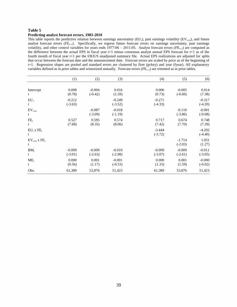
39

Table 5 Predicting analyst forecast errors, 1983-2010 This table reports the predictive relation between earnings uncertainty (EUt), past earnings volatility (EVt-4,t), and future

analyst forecast errors (FEt+1). Specifically, we regress future forecast errors on earnings uncertainty, past earnings

volatility, and other control variables for years ends 1977:06 – 2011:05. Analyst forecast errors (FEt+1) are computed as

the difference between the actual EPS in fiscal year t+1 minus consensus analyst annual EPS forecast for t+1 as of the

fourth month of fiscal year t+1 per the I/B/E/S unadjusted summary file. Actual EPS realizations are adjusted for splits

that occur between the forecast date and the announcement date. Forecast errors are scaled by price as of the beginning of

t+1. Regression slopes are pooled and standard errors are clustered by firm (gvkey) and year (fyear). All explanatory

variables defined as in prior tables and winsorized annually. Forecast errors (FEt+1) are trimmed as in prior tables.

(1) (2) (3) (4) (5) (6)

Intercept 0.008 -0.004 0.016 0.006 -0.005 0.014

t (0.78) (-0.42) (1.59) (0.73) (-0.60) (7.38)

EU t -0.212 -0.249 -0.271 -0.317

t (-3.63) (-3.52) (-4.33) (-4.20)

EVt-4,t -0.087 -0.018 -0.110 -0.001

t (-3.09) (-1.19) (-3.86) (-0.08)

FEt 0.527 0.595 0.574 0.717 0.674 0.748

t (7.68) (8.35) (8.06) (7.42) (7.70) (7.39)

EUt x FEt -3.444 -4.292

t (-3.72) (-4.40)

EVt-4,t x FEt -1.714 1.051

t (-2.03) (1.27)

BMt -0.009 -0.009 -0.010 -0.009 -0.009 -0.011

t (-3.01) (-2.63) (-2.98) (-3.07) (-2.61) (-3.05)

MEt 0.000 0.001 -0.001 0.000 0.001 -0.000

t (0.56) (1.17) (-0.53) (1.33) (1.59) (-0.02)

Obs.

61,389 53,876 51,423 61,389 53,876 51,423

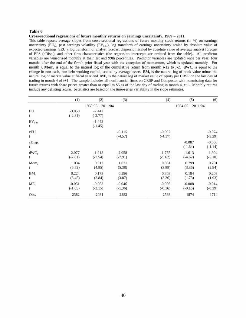
40

Table 6 Cross-sectional regressions of future monthly returns on earnings uncertainty, 1969 – 2011 This table reports average slopes from cross-sectional regressions of future monthly stock returns (in %) on earnings

uncertainty (EUt), past earnings volatility (EVt-4,t), log transform of earnings uncertainty scaled by absolute value of

expected earnings (cEUt), log transform of analyst forecast dispersion scaled by absolute value of average analyst forecast

of EPS (cDispt), and other firm characteristics (the regression intercepts are omitted from the table). All predictor

variables are winsorized monthly at their 1st and 99th percentiles. Predictor variables are updated once per year, four

months after the end of the firm’s prior fiscal year with the exception of momentum, which is updated monthly. For

month j, Momt is equal to the natural log of the cumulative return from month j-12 to j-2. dWCt is equal to the

change in non-cash, non-debt working capital, scaled by average assets. BMt is the natural log of book value minus the

natural log of market value at fiscal year end. MEt is the nature log of market value of equity per CRSP on the last day of

trading in month 4 of t+1. The sample includes all nonfinancial firms on CRSP and Compustat with nonmissing data for

future returns with share prices greater than or equal to $5 as of the last day of trading in month 4, t+1. Monthly returns

include any delisting return. t-statistics are based on the time-series variability in the slope estimates. (1) (2) (3) (4) (5) (6)

1969:05 – 2011:04 1984:05 – 2011:04

EU t -3.050 -2.442

t (-2.81) (-2.77)

EVt-4,t -1.443

t (-1.45)

cEUt -0.115 -0.097 -0.074

t (-4.57) (-4.17) (-3.29)

cDispt -0.087 -0.060

t (-1.64) (-1.14)

dWCt -2.077 -1.918 -2.058 -1.755 -1.613 -1.904

t (-7.81) (-7.54) (-7.91) (-5.62) (-4.62) (-5.10)

Momt 1.034 0.912 1.021 0.861 0.799 0.701

t (5.52) (4.85) (5.38) (3.88) (3.36) (2.94)

BMt 0.224 0.173 0.296 0.303 0.184 0.203

t (3.45) (2.84) (3.87) (3.26) (1.73) (1.93)

MEt -0.051 -0.063 -0.046 -0.006 -0.008 -0.014

t (-1.65) (-2.15) (-1.36) (-0.16) (-0.16) (-0.29)

Obs.

2382 2031 2382 2593 1874 1714

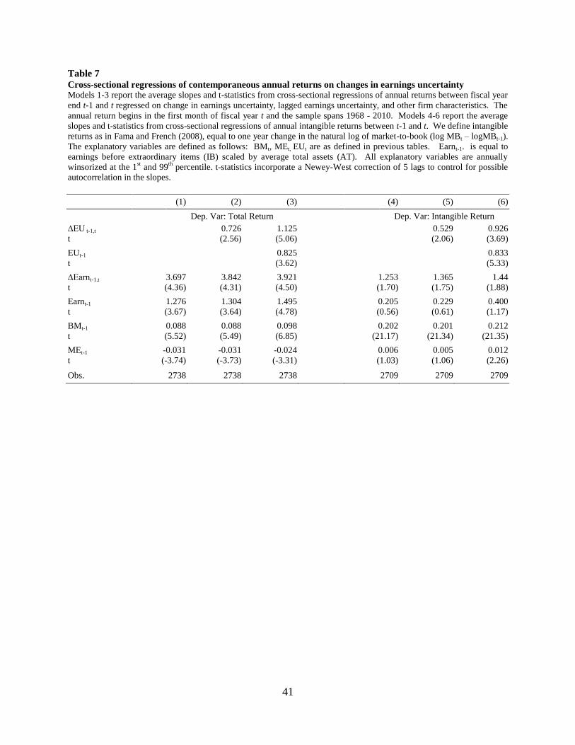
41

Table 7 Cross-sectional regressions of contemporaneous annual returns on changes in earnings uncertainty Models 1-3 report the average slopes and t-statistics from cross-sectional regressions of annual returns between fiscal year

end t-1 and t regressed on change in earnings uncertainty, lagged earnings uncertainty, and other firm characteristics. The

annual return begins in the first month of fiscal year t and the sample spans 1968 - 2010. Models 4-6 report the average

slopes and t-statistics from cross-sectional regressions of annual intangible returns between t-1 and t. We define intangible

returns as in Fama and French (2008), equal to one year change in the natural log of market-to-book (log MBt – logMBt-1).

The explanatory variables are defined as follows: BMt, MEt, EUt are as defined in previous tables. Earnt-1. is equal to

earnings before extraordinary items (IB) scaled by average total assets (AT). All explanatory variables are annually

winsorized at the 1st and 99

th percentile. t-statistics incorporate a Newey-West correction of 5 lags to control for possible

autocorrelation in the slopes.

(1) (2) (3) (4) (5) (6)

Dep. Var: Total Return Dep. Var: Intangible Return

∆EU t-1,t 0.726 1.125 0.529 0.926

t (2.56) (5.06) (2.06) (3.69)

EUt-1 0.825 0.833

t (3.62) (5.33)

∆Earnt-1,t 3.697 3.842 3.921 1.253 1.365 1.44

t (4.36) (4.31) (4.50) (1.70) (1.75) (1.88)

Earnt-1 1.276 1.304 1.495 0.205 0.229 0.400

t (3.67) (3.64) (4.78) (0.56) (0.61) (1.17)

BMt-1 0.088 0.088 0.098 0.202 0.201 0.212

t (5.52) (5.49) (6.85) (21.17) (21.34) (21.35)

MEt-1 -0.031 -0.031 -0.024 0.006 0.005 0.012

t (-3.74) (-3.73) (-3.31) (1.03) (1.06) (2.26)

Obs.

2738 2738 2738 2709 2709 2709

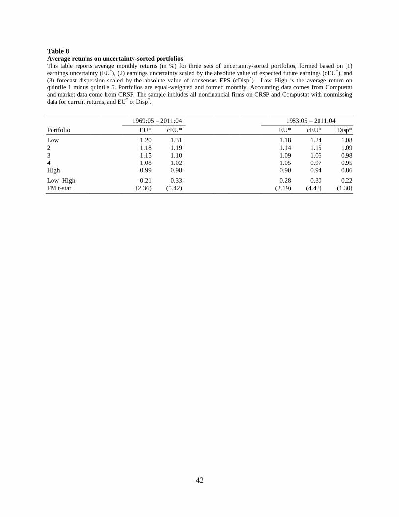
42

Table 8 Average returns on uncertainty-sorted portfolios This table reports average monthly returns (in %) for three sets of uncertainty-sorted portfolios, formed based on (1)

earnings uncertainty (EU*), (2) earnings uncertainty scaled by the absolute value of expected future earnings (cEU

*), and

(3) forecast dispersion scaled by the absolute value of consensus EPS (cDisp*). Low–High is the average return on

quintile 1 minus quintile 5. Portfolios are equal-weighted and formed monthly. Accounting data comes from Compustat

and market data come from CRSP. The sample includes all nonfinancial firms on CRSP and Compustat with nonmissing

data for current returns, and EU* or Disp

*.

1969:05 – 2011:04 1983:05 – 2011:04

Portfolio EU* cEU* EU* cEU* Disp*

Low 1.20 1.31 1.18 1.24 1.08

2 1.18 1.19 1.14 1.15 1.09

3 1.15 1.10 1.09 1.06 0.98

4 1.08 1.02 1.05 0.97 0.95

High 0.99 0.98 0.90 0.94 0.86

Low–High 0.21 0.33 0.28 0.30 0.22

FM t-stat (2.36) (5.42) (2.19) (4.43) (1.30)