Roadmap to the morphological instabilities of a stretched ...
55
Noname manuscript No. (will be inserted by the editor) Roadmap to the morphological instabilities of a stretched twisted ribbon Julien Chopin · Vincent D´ emery ? · Benny Davidovitch March 1, 2014 Abstract We address the mechanics of an elastic ribbon subjected to twist and tensile load. Motivated by the classical work of Green [1, 2] and a recent experi- ment [3] that discovered a plethora of morphological instabilities, we introduce a comprehensive theoretical framework through which we construct a 4D phase dia- gram of this basic system, spanned by the exerted twist and tension, as well as the thickness and length of the ribbon. Different types of instabilities appear in various “corners” of this 4D parameter space, and are addressed through distinct types of asymptotic methods. Our theory introduces three instruments, whose concerted employment is necessary to provide an exhaustive study of the various parameter regimes: (i) a covariant form of the F¨ oppl-von K´ arm´ an (cFvK) equations – nec- essary to account for the large deflection of the highly-symmetric helicoidal shape from planarity, and the buckling instability of the ribbon in the transverse direc- tion; (ii) a far from threshold (FT) analysis – which describes a state in which a longitudinally-wrinkled zone expands throughout the ribbon and allows it to retain a helicoidal shape with negligible compression; (iii) finally, we introduce an asymptotic isometry equation that characterizes the energetic competition be- tween various types of states through which a twisted ribbon becomes strainless in the singular limit of zero thickness and no tension. Keywords Buckling and wrinkling · Far from threshold · Isometry · Helicoid ? J.C and V.D. have contributed equally to this work. Julien Chopin Civil Engineering Department, COPPE, Universidade Federal do Rio de Janeiro, 21941-972, Rio de Janeiro RJ, Brazil and Department of Physics, Clark University, Worcester, Massachusetts 01610, USA E-mail: [email protected] Vincent D´ emery Physics Department, University of Massachusetts, Amherst MA 01003, USA E-mail: [email protected] Benny Davidovitch Physics Department, University of Massachusetts, Amherst MA 01003, USA E-mail: [email protected]
Transcript of Roadmap to the morphological instabilities of a stretched ...

Noname manuscript No.(will be inserted by the editor)
Roadmap to the morphological instabilities of astretched twisted ribbon
Julien Chopin · Vincent Demery? · BennyDavidovitch
March 1, 2014
Abstract We address the mechanics of an elastic ribbon subjected to twist andtensile load. Motivated by the classical work of Green [1,2] and a recent experi-ment [3] that discovered a plethora of morphological instabilities, we introduce acomprehensive theoretical framework through which we construct a 4D phase dia-gram of this basic system, spanned by the exerted twist and tension, as well as thethickness and length of the ribbon. Different types of instabilities appear in various“corners” of this 4D parameter space, and are addressed through distinct types ofasymptotic methods. Our theory introduces three instruments, whose concertedemployment is necessary to provide an exhaustive study of the various parameterregimes: (i) a covariant form of the Foppl-von Karman (cFvK) equations – nec-essary to account for the large deflection of the highly-symmetric helicoidal shapefrom planarity, and the buckling instability of the ribbon in the transverse direc-tion; (ii) a far from threshold (FT) analysis – which describes a state in whicha longitudinally-wrinkled zone expands throughout the ribbon and allows it toretain a helicoidal shape with negligible compression; (iii) finally, we introducean asymptotic isometry equation that characterizes the energetic competition be-tween various types of states through which a twisted ribbon becomes strainlessin the singular limit of zero thickness and no tension.
Keywords Buckling and wrinkling · Far from threshold · Isometry · Helicoid
? J.C and V.D. have contributed equally to this work.
Julien ChopinCivil Engineering Department, COPPE, Universidade Federal do Rio de Janeiro,21941-972, Rio de Janeiro RJ, Braziland Department of Physics, Clark University, Worcester, Massachusetts 01610, USAE-mail: [email protected]
Vincent DemeryPhysics Department, University of Massachusetts, Amherst MA 01003, USAE-mail: [email protected]
Benny DavidovitchPhysics Department, University of Massachusetts, Amherst MA 01003, USAE-mail: [email protected]

2 Julien Chopin et al.
ssFvK equations “small-slope” (standard) Foppl-von Karman equa-tions
cFvK equations covariant Foppl-von Karman equationst, W, L thickness, width and length of the ribbon (non-
italicized quantities are dimensionfull)t, W = 1, L thickness, width and length normalized by the widthν Poisson ratio
E, Y, B = Yt2
12(1−ν2) Young, stretching and bending modulus
Y = 1, B = t2
12(1−ν2) stretching and bending modulus, normalized by thestretching modulus
T = T/Y tensionθ, η = θ/L twist angle and normalized twist(x, y, z) cartesian basiss, r material coordinates (longitudinal and transverse)z(s, r) out of plane displacement (of the helicoid) in the
small-slope approximationX(s, r) surface vectorn unit normal to the surface
σαβ stress tensorεαβ strain tensorgαβ metric tensorcαβ curvature tensor
Aαβγδ elastic tensor∂α, Dα partial and covariant derivativesH, K mean and Gaussian curvaturesζ infinitesimal amplitude of the perturbation in linear
stability analysisz1(s, r) normal component of an infinitesimal perturbation to
the helicoidal shapeηlon, λlon longitudinal instability threshold and wavelengthηtr, λtr transverse instability threshold and wavelengthα = η2/T confinement parameterαlon threshold confinement for the longitudinal instability.rwr (half the) width of the longitudinally wrinkled zone∆α = α− 24 distance to the threshold confinementf(r) amplitude of the longitudinal wrinklesUhel, UFT elastic energies (per length) of the helicoid and the
far from threshold longitudinally wrinkled stateUdom, Usub dominant and subdominant (with respect to t) parts
of UFT
Xcl(s) ribbon centerlinet = dXcl(s)/ds tangent vector in the ribbon’s midplaner(s) the normal to the tangent vector
b(s) Frenet binormal to the curve Xcl(s)τ(s), κ(s) torsion and curvature of Xcl(s)

Roadmap to the morphological instabilities of a stretched twisted ribbon 3
Fig. 1 Left: Typical morphologies of ribbons subjected to twist and stretching: (a) helicoid,(b,c) longitudinally wrinkled helicoid, (d) creased helicoid, (e) formation of loops and self-contact zones, (f) cylindrical wrapping, (g) transverse buckling and (h) twisted towel showstransverse buckling/wrinkling. Right: (i) Experimental phase diagram in the tension-twistplane, adapted from [3]. The descriptive words are from the original diagram [3].
1 Introduction
1.1 Overview
A ribbon is a thin, long solid sheet, whose thickness and length, normalized by thewidth, satisfy:
thickness : t� 1 ; length: L� 1 . (1)
The large contrast between thickness, width, and length, distinguishes ribbonsfrom other types of thin objects, such as rods (t ∼ 1, L � 1) and plates (t �1, L ∼ 1), and underlies their complex response to simple mechanical loads. Theunique nature of mechanics of ribbons is demonstrated in Fig. 1, which shows a fewtypical morphologies of ribbons that are subjected to twist and stretching. Thisbasic loading is characterized by two small dimensionless parameters (see Fig. 2):
twist : η � 1 ; tension: T � 1 , (2)
where η is the average twist (per length), and T is the tension, normalized by thestretching modulus 1.
Most theoretical approaches to this problem consider the behavior of a realribbon through the asymptotic “ribbon limit”, of an ideal ribbon with infinitesimalthickness and infinite length: t→ 0, L→∞. A first approach, introduced by Green[1,2], assumes that the ribbon’s shape is close to a helicoid (Fig. 1a), such that theribbon is strained, and may therefore become wrinkled or buckled at certain valuesof η and T (Fig. 1b,c,g,h) [4,5]. A second approach to the ribbon limit, initiated
1 Our convention in this paper is to normalize lengths by the ribbon width W, and stressesby the stretching modulus Y, which is the product of the Young modulus and the ribbon’sthickness (non-italicized fonts are used for dimensionfull parameters and italicized fonts for di-mensionless parameters). Thus, the actual thickness and length of the ribbon are, respectively,t = t ·W and L = L ·W, the actual force that pulls on the short edges is T · YW, and theactual tension due to this pulling force is T = T ·Y.

4 Julien Chopin et al.
Fig. 2 A ribbon of length L and width W (and thickness t, not shown) is submitted to atension T and a twist angle θ; the twist parameter is defined as η = θ/L = θW/L. Thelongitudinal and transverse material coordinates are s and r, respectively. n is the unit normalto the surface, (x, y, z) is the standard basis, (x, y) being the plane of the untwisted ribbon.
by Sadowsky [6] and revived recently by Korte et al. [7], considers the ribbon as an“inextensible” strip, whose shape is close to a creased helicoid – an isometric (i.e.strainless) map of the unstretched, untwisted ribbon (Fig. 1c). A third approach,which may be valid for sufficiently small twist, assumes that the stretched-twistedribbon is similar to the wrinkled shape of a planar, purely stretched rectangularsheet, with a wrinkle’s wavelength that vanishes as t→ 0 and increases with L [8].Finally, considering the ribbon as a rod with highly anisotropic cross section, onemay approach the problem by solving the Kirchoff rod’s equations and carryingout stability analysis of the solution, obtaining unstable modes that resemble thelooped shape (Fig. 1e) [9].
A recent experiment [3], which we briefly describe in Subsec. 1.2, revealed someof the predicted patterns and indicated the validity of the corresponding theoreticalapproaches at certain regimes of the parameter plane (T, η) (Fig. 1). Motivated bythis development, we introduce in this paper a unifying framework that clarifies thehidden assumptions underlying each theoretical approach, and identifies its validityrange in the (T, η) plane for given values of t and L. Specifically, we show that asingle theory, based on a covariant form of the Foppl–von Karman (FvK) equationsof elastic sheets, describes the parameter space (T, η, t, L−1) of a stretched twistedribbon (where all parameters are assumed small, Eqs. (1,2)); various “corners” ofthis 4D parameter space are described by distinct singular limits of the governingequations of this theory, which yield qualitatively different types of patterns. Thisrealization is illustrated in Fig. 3, which depicts the projection of the 4D parameterspace on the (T, η) plane, and indicates several regimes that are governed bydifferent types of asymptotic expansions.

Roadmap to the morphological instabilities of a stretched twisted ribbon 5
1.2 Experimental observations
The authors of [3] used mylar ribbons, subjected them to various levels of tensileload and twist, and recorded the observed patterns in the parameter plane (T, η),which we reproduce in Fig. 1. The experimental results indicate the existence ofthree major regimes that meet at a “λ-point” (Tλ, ηλ). We describe below themorphology in each of the three regimes and the behavior of the curves thatseparate them:
• The helicoidal shape is observed if the twist η is sufficiently small. For T < Tλ,the helicoid is observed for η < ηlon, where ηlon ≈
√24T is nearly independent on
the ribbon’s thickness t. For T > Tλ, the helicoid is observed for η < ηtr, whereηtr exhibits a strong dependence on the thickness (ηtr ∼
√t) and a weak (or none)
dependence on the tension T . The qualitative change at the λ-point reflects twosharply different mechanisms by which the helicoidal shape becomes unstable.
• As the twist exceeds ηlon (for T < Tλ), the ribbon develops longitudinalwrinkles in a narrow zone around its centerline. Both the wrinkle’s wavelengthand the width of the wrinkled zone scale as ∼ (t/
√T )1/2. This observation is in
excellent agreement with Green’s characterization of the helicoidal state, based onthe familiar FvK equations of elastic sheets [2]. Green’s solution shows that thelongitudinal stress at the helicoidal state becomes compressive around the ribbon’scenterline if η >
√24T , and the linear stability analysis of Coman and Bassom [5]
yields the unstable wrinkling mode that relax the longitudinal compression.
• As the twist exceeds ηtr (for T > Tλ), the ribbon becomes buckled in thetransverse direction, indicating the existence of transverse compression at the heli-coidal state that increases with η. A transverse instability cannot be explained byGreen’s calculation, which yields no transverse stress [2], but has been predictedby Mockensturm [4], who studied the stability of the helicoidal state using the fullnonlinear elasticity equations. Alas, Mockensturm’s results were only numericaland did not reveal the scaling behavior ηtr ∼
√t observed in [3]. Furthermore,
the nonlinear elasticity equations in [4] account for the inevitable geometric effect(large deflection of the twisted ribbon from its flat state), as well as a mechani-cal effect (non-Hookean stress-strain relation), whereas only the geometric effectseems to be relevant for the experimental conditions of [3].
• Turning back to T < Tλ, the ribbon exhibit two striking features as the twist ηis increased above the threshold value ηlon. First, the longutinally-wrinkled ribbontransforms to a shape that resembles the creased helicoid state predicted by [7];this transformation becomes more prominent at small tension (i.e. decreasing Tat a fixed value of η). Second, the ribbon undergoes a sharp, secondary transition,described in [3] as similar to the “looping” transition of rods [9,10,11,12]. At agiven tension T < Tλ, this secondary instability occurs at a critical twist valuethat decreases with T , but is nevertheless significantly larger than ηlon ≈
√24T .
• Finally, the parameter regime in the (T, η) plane bounded from below by thisseconday instability (for T < Tλ) and by the transverse buckling instability (forT > Tλ), is characterized by hysteresis and dominated by the formation of loopsand self-contact zones along the ribbon.
In a recent commentary [13], Santangelo recognized the challenge and the op-portunity introduced to us by this experiment: “Above all, this paper is a challengeto theorists. Here, we have an experimental system that exhibits a wealth of mor-
6 Julien Chopin et al.
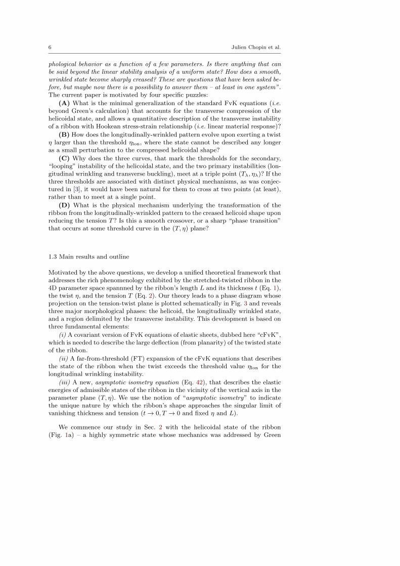
phological behavior as a function of a few parameters. Is there anything that canbe said beyond the linear stability analysis of a uniform state? How does a smooth,wrinkled state become sharply creased? These are questions that have been asked be-fore, but maybe now there is a possibility to answer them – at least in one system”.The current paper is motivated by four specific puzzles:
(A) What is the minimal generalization of the standard FvK equations (i.e.beyond Green’s calculation) that accounts for the transverse compression of thehelicoidal state, and allows a quantitative description of the transverse instabilityof a ribbon with Hookean stress-strain relationship (i.e. linear material response)?
(B) How does the longitudinally-wrinkled pattern evolve upon exerting a twistη larger than the threshold ηlon, where the state cannot be described any longeras a small perturbation to the compressed helicoidal shape?
(C) Why does the three curves, that mark the thresholds for the secondary,“looping” instability of the helicoidal state, and the two primary instabilities (lon-gitudinal wrinkling and transverse buckling), meet at a triple point (Tλ, ηλ)? If thethree thresholds are associated with distinct physical mechanisms, as was conjec-tured in [3], it would have been natural for them to cross at two points (at least),rather than to meet at a single point.
(D) What is the physical mechanism underlying the transformation of theribbon from the longitudinally-wrinkled pattern to the creased helicoid shape uponreducing the tension T? Is this a smooth crossover, or a sharp “phase transition”that occurs at some threshold curve in the (T, η) plane?
1.3 Main results and outline
Motivated by the above questions, we develop a unified theoretical framework thataddresses the rich phenomenology exhibited by the stretched-twisted ribbon in the4D parameter space spannned by the ribbon’s length L and its thickness t (Eq. 1),the twist η, and the tension T (Eq. 2). Our theory leads to a phase diagram whoseprojection on the tension-twist plane is plotted schematically in Fig. 3 and revealsthree major morphological phases: the helicoid, the longitudinally wrinkled state,and a region delimited by the transverse instability. This development is based onthree fundamental elements:
(i) A covariant version of FvK equations of elastic sheets, dubbed here “cFvK”,which is needed to describe the large deflection (from planarity) of the twisted stateof the ribbon.
(ii) A far-from-threshold (FT) expansion of the cFvK equations that describesthe state of the ribbon when the twist exceeds the threshold value ηlon for thelongitudinal wrinkling instability.
(iii) A new, asymptotic isometry equation (Eq. 42), that describes the elasticenergies of admissible states of the ribbon in the vicinity of the vertical axis in theparameter plane (T, η). We use the notion of “asymptotic isometry” to indicatethe unique nature by which the ribbon’s shape approaches the singular limit ofvanishing thickness and tension (t→ 0, T → 0 and fixed η and L).
We commence our study in Sec. 2 with the helicoidal state of the ribbon(Fig. 1a) – a highly symmetric state whose mechanics was addressed by Green
Roadmap to the morphological instabilities of a stretched twisted ribbon 7
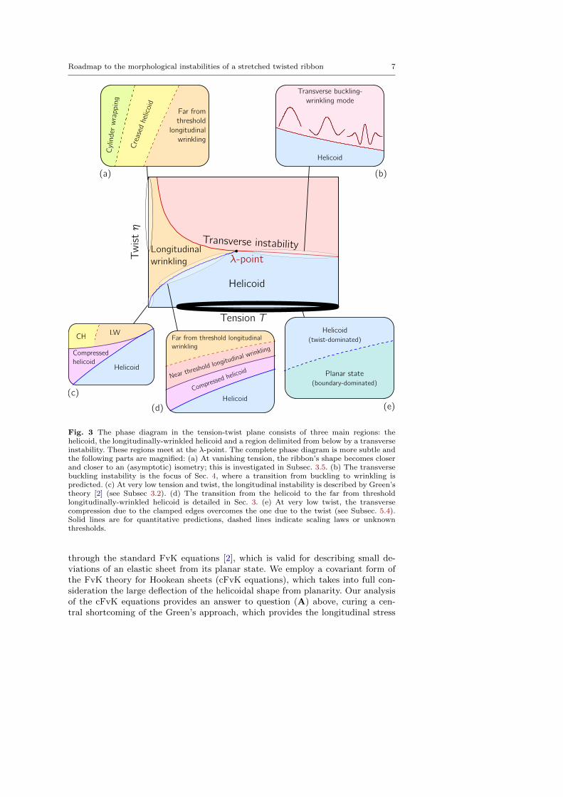
Fig. 3 The phase diagram in the tension-twist plane consists of three main regions: thehelicoid, the longitudinally-wrinkled helicoid and a region delimited from below by a transverseinstability. These regions meet at the λ-point. The complete phase diagram is more subtle andthe following parts are magnified: (a) At vanishing tension, the ribbon’s shape becomes closerand closer to an (asymptotic) isometry; this is investigated in Subsec. 3.5. (b) The transversebuckling instability is the focus of Sec. 4, where a transition from buckling to wrinkling ispredicted. (c) At very low tension and twist, the longitudinal instability is described by Green’stheory [2] (see Subsec 3.2). (d) The transition from the helicoid to the far from thresholdlongitudinally-wrinkled helicoid is detailed in Sec. 3. (e) At very low twist, the transversecompression due to the clamped edges overcomes the one due to the twist (see Subsec. 5.4).Solid lines are for quantitative predictions, dashed lines indicate scaling laws or unknownthresholds.
through the standard FvK equations [2], which is valid for describing small de-viations of an elastic sheet from its planar state. We employ a covariant form ofthe FvK theory for Hookean sheets (cFvK equations), which takes into full con-sideration the large deflection of the helicoidal shape from planarity. Our analysisof the cFvK equations provides an answer to question (A) above, curing a cen-tral shortcoming of the Green’s approach, which provides the longitudinal stress

8 Julien Chopin et al.
but predicts a vanishing transverse stress. The cFvK equations of the helicoidalstate yield both components of the stress tensor, and show that the magnitudeof the transverse stress is nonzero, albeit much smaller than the longitudinal one.Another crucial difference between the two stress components of the helicoidalstate pertains to their sign: the transverse stress is compressive throughout thewhole ribbon, everywhere in the parameter plane (T, η); in contrast, the longi-tudinal stress is compressive in a zone around the ribbon’s centerline only forη > ηlon ≈
√24T . The compressive nature of the stress components gives rise to
buckling and wrinkling instabilities that we address in Secs. 3 and 4.
In Sec. 3 we address the wrinkling instability that relaxes the longitudinal com-pression for η >
√24T . Noticing that the longitudinally-compressed zone of the
helicoidal state broadens upon increasing the ratio α = η2/T , we recognize a closeanalogy between the longitudinally-wrinkled state of the ribbon and wrinklingphenomena in radially-stretched sheets [14,15,16], where the size of the wrinkledzone depends on a confinement parameter, defined by a ratio between the loads ex-erted on the sheet. Exploiting this analogy further, we find that the longitudinally-wrinkled ribbon at η > ηlon is described by a far-from-threshold (FT) expansion ofthe cFvK equations, where the longitudinal stress (at any given α > 24) becomescompression-free in the singular limit of an infinitely thin ribbon, t→ 0. The FTtheory predicts that the broadening of the wrinkled zone with the confinementα is dramatically larger than the prediction of a near-threshold (NT) approach,which is based on a perturbative (amplitude) expansion around the compressivehelicoidal state. Our FT theory of the longitudinally wrinkled state provides ananswer to question (B) in the above list.
Analyzing the FT expansion in the two limits α → 24 (i.e. η →√
24T ), andα→∞ (i.e. fixed η and T → 0), elucidates further the nature of the longitudinallywrinkled state. In the limit α → 24, plotted schematically in Fig. 3(a), we findthat the FT regime prevails in the domain η >
√24T in the (T, η) plane, whereas
the NT parameter regime, at which the state is described as a perturbation to theunwrinkled helicoidal state, shrinks to a narrow sliver close to the threshold curveas the thickness vanishes, t → 0. Analyzing the other limit, α → ∞, we showthat the longitudinally-wrinkled state becomes an asymptotic isometry, where thestrain vanishes throughout the twisted ribbon. In Sec. 5 we expand more on themeaning and implications of asymptotic isometries for a stretched-twisted ribbon.The FT analysis of the two limits, α → 24 and α → ∞, reveals the intricate me-chanics of a ribbon subjected to twist η, whereby the longitudinally wrinkled stateentails a continuous trajectory in the (T, η) plane, from a strainless deformation(at T → 0) to a fully strained helicoidal shape (at T ≥ η2/24).
In Sec. 4 we turn to the transverse instability, capitalizing on our results fromSecs. 2 and 3. First, we note that the transverse stress is compressive everywherein the (T, η) plane; second, we note that it is obscured by the longitudinal stress.These two features imply that the threshold for the transverse instability occurs ata curve ηtr(T ) in the (T, η) plane, that divides it into two parts: In the first part,defined by the inequality ηtr(T ) <
√24T , the longitudinal stress is purely tensile,
and the transverse instability appears as a primary instability of the helicoidalstate; in the second part, defined by ηtr(T ) >
√24T , the transverse instability
is preceeded by the longitudinal instability, and thus materializes as a secondaryinstability of the helicoidal state. We conclude that the “looping” instability ob-served in [3] does not stem from a new physical mechanism, but simply reflects
Roadmap to the morphological instabilities of a stretched twisted ribbon 9
the change in nature of the transverse instability when the threshold line ηtr(T )crosses the curve ηlon =
√24T that separates the longitudinally-compressed and
longitudinally-tensed domains of the (T, η) plane. Thus, the emergence of the“triple” point (Tλ, ηλ) is not mysterious, but comes naturally as the intersectionof these two curves in the (T, η) plane. This result answers question (C) in ourlist.
The cFvK equations, together with the FT analysis of the longitudinally-wrinkled state in Sec. 3, allow us to compute the deformation modes that relax thetransverse compression. Two results from this stability analysis are noteworthy.First, assuming an infinitely long ribbon, we find that the threshold curve satisfiesηtr(T ) ∼ t/
√T in both the ”low”-tension regime (T < Tλ) and ”large”-tension
regime (T > Tλ), albeit with different numerical pre-factors. This theoretical pre-diction is in strong accord with the experimental data for the transverse bucklinginstability and the “looping” instability in [3]. Second, we find that the length ofthe ribbon has a dramatic effect on the dependence of the λ-point on the ribbon’sthickness t, and – more importantly – on the spatial structure of the transverseinstability. Specifically, we predict that if L−2 � t� 1, the transverse instabilityis buckling, and if t� L−2 � 1, it may give rise to a wrinkling pattern, similarlyto a stretched, untwisted ribbon [8], with a characteristic wavelength λtr < 1 thatbecomes smaller as T increases. This “buckling to wrinkling” transition is depictedin Fig. 3c.
In Sec. 5 we turn to the edges of the (T, η) plane, namely, the vicinity of thevertical and horizontal axes: (T = 0, η) and (T, η= 0), respctively. In order to ad-dress the first limit, we briefly review the work of Korte et al. [7] that predictedand analyzed the creased helicoid state. We discuss the asymptotic isometry exhib-ited by the creased helicoid state in the singular limit t→ 0, T → 0, and contrastit with the asymptotic isometry of the longitudinally wrinkled state, which wasnoted first in Sec. 3. We elucidate an important implication of the asymptoticisometry equation derived in Sec. 3, which provides a general framework for an-alyzing morphological transitions between various types of asymptotic isometriesin the neighborhood of the singular hyper-plane t = 0, T = 0 in the 4D parame-ter space (T, η, t, L). As a consequence of this discussion, we propose the scenarioillustrated in Fig. 3b, where the longitudinally wrinkled state undergoes a sharptransition to the creased helicoid state in the vicinity of the (T = 0, η) line. Thus,while our discussion here is less rigorous than in the previous sections (due to thecomplexity of the creased helicoid state [7]), we nevertheless provide a heuristicanswer to question (D) in our list.
Since the characterization of the creased helicoid state in [7] is based on theSadowsky’s formalism of inextensible strips rather than on the FvK theory ofelastic sheets, we use this opportunity to elaborate on the basic difference betweenthe “rod-like” and “plate-like” approaches to the mechanics of ribbons. We alsorecall another rod-like approach, based on implementation of the classical Kirchoffequations for a rod with anisotropic cross section [9,10,11,12], and explain whyit is not suitable to study the ribbon limit (Eq. 1) that corresponds to a rodwith highly anisotropic cross section. Finally, we turn to the vicinity of the pure-stretching line, (η = 0, T ), and address the parameter regime where the twist ηis so small that the ribbon does not accommodate a helicoidal shape. We providea heuristic, energy-based argument, which indicates that the helicoidal state is

10 Julien Chopin et al.
established if the twist η is larger than a minimal value that is proportional to thePoisson ratio, and scales as 1/
√L.
Each of Secs. 2-5 starts with an overview that provides a detailed description ofthe main results in that section. Given the considerable length of this manuscript,a first reading may be focused on these overview subsections only (2.1,3.1,4.1,5.1),followed by Sec. 6, where we describe experimental challenges and propose a listof theoretical questions inspired by our work.
2 Helicoidal state
2.1 Overview
The helicoidal state has been studied by Green [2], who computed its stress fieldusing the standard version of the FvK equations (8,9). This familiar form, to whichwe refer here as the ss-FvK equations (“ss” stands for “small slope”) is valid forsmall deflections of elastic sheets from their planar state [17]. The Green’s stress,Eqs. (21,22), has a longitudinal component that contains terms proportional toT and to η2, and no transverse component. However, the experiments of [3], aswell as numerical simulations [18,19], have exhibited a buckling instability of thehelicoidal state in the transverse direction, indicating the presence of transversecompression. One may suspect that the absence of transverse component in Green’sstress indicates that the magnitude of this component is small, being proportionalto a high power of the twist η, which cannot be captured by the ss-FvK equations.
Here we resort to a covariant form of the FvK equations, which we call “cFvK”[20,21,22], that does not assume a planar reference state, and is thus capable ofdescribing large deviations from a planar state. Notably, the large deflection ofthe helicoidal state from planarity does not involve large strains. Hence, as longas T, η � 1, we consider a ribbon with Hookean response, namely – linear stress-strain relationship 2. Solving the cFvK equations for the helicoidal state, we getthe following expressions for the stress field in the longitudinal (s) and transverse(r) directions:
σsshel(r) = T +η2
2
(r2 − 1
12
), (3)
σrrhel(r) =η2
2
(r2 − 1
4
)[T +
η2
4
(r2 +
1
12
)], (4)
The longitudinal component is exactly the one found by Green [2], whereas thetransverse component is nonzero, albeit of small magnitude: σrrhel ∼ η2σsshel, whichexplains why it is missed by the ss-FvK equations. The transverse stress arisesfrom a subtle coupling between the longitudinal stress and the geometry of theribbon.
As Eqs. (3,4) show, the longitudinal stress σsshel(r) is compressive close to thecenterline r = 0 if η2 > 24T , whereas the transverse stress σrrhel(r) is compressiveeverywhere in the ribbon for any (T, η). The compressive nature of σsshel(r) and
2 In this sense, our approach is simpler than Mockensturm’s [4], which assumed a non-Hookean response and employed numerical methods to find the stress of the helicoidal stateand to analyze its stability.

Roadmap to the morphological instabilities of a stretched twisted ribbon 11
σrrhel(r) leads to buckling and wrinkling instabilities that we adress in the nextsections.
In Sec. 2.2 we review the (standard) ss-FvK equations, and their helicoidalsolution found by Green [2]. In Sec. 2.3 we proceed to derive the cFvK equations,following [22], and use this covariant formalism to determine the stress in thehelicoidal state.
2.2 Small slope approximation and the Green solution
2.2.1 Small-slope FvK equations
We review briefly the standard ss-FvK equations, using some basic concepts ofdifferential geometry that will allow us to introduce their covariant version in thenext subsection. Assuming a small deviation from a plane, a sheet is defined byits out-of-plane displacement z(s, r) and its in-plane displacements us(s, r) andur(s, r); where s and r are the material coordinates. In this configuration, thestrain is given by
εαβ =1
2[∂αuβ + ∂βuα + (∂αz)(∂βz)] . (5)
The greek indices α and β take the values s or r. We define the curvature tensorand the mean curvature as:
cαβ = ∂α∂βz, (6)
H =1
2cαα =
1
2∆z, (7)
where we use the Einstein summation convention, such that cαα is the trace of thecurvature tensor. The use of upper or lower indices corresponds to the nature ofthe tensor (contravariant or covariant, respectively), which will become relevant inthe next subsection. The ss-FvK equations express the force balance in the normaldirection (z) and the in-plane directions (s, r), and involve the curvature tensorand the stress tensor σαβ(s, r):
cαβσαβ = 2B∆H, (8)
∂ασαβ = 0, (9)
where B = t2/[12(1−ν2)] is the bending modulus of the sheet 3. The stress-strainrelationship is given by the Hook’s law (linear material response):
σαβ =1
1 + νεαβ +
ν
1− ν2 εγγδαβ . (10)
where we used the Kronecker symbol δαβ .
3 Recall that we normalize stresses by the stretching modulus Y and lengths by the ribbon’swidth W. The dimensionfull bending modulus is thus: (t2/(12(1− ν2)) YW2.

12 Julien Chopin et al.
2.2.2 Green solution for the helicoid
We now apply the ss-FvK equations (8,9) to find the stress in the helicoidal state.Since this formalism assumes a small deviation of the ribbon from the plane, weapproximate the helicoidal shape through:
z(s, r) = ηsr , (11)
obtained by Taylor expansion of the z-coordinate of the full helicoidal shape, givenbelow in Eq. (29), for |s| � η−1. Its corresponding curvature tensor is:
cαβ = η
(0 11 0
), (12)
leading to the mean curvature H = 0. The force balance equations (8-9) now read:
σsr = 0, (13)
∂sσss = 0, (14)
∂rσrr = 0. (15)
The ss-FvK equations are supplemented by two boundary conditions: The longi-tudinal stress must match the tensile load exerted on the short edges, whereas thelong edges are free, namely: ∫ 1/2
−1/2
σss(r)dr = T, (16)
σrr(r = ±1/2) = 0. (17)
Since Eq. (15) implies that the transverse stress is uniform across the ribbon, theboundary condition (17) implies that it is identically zero:
σrr(r) = 0. (18)
Now, Eq. (14) and the Hooke’s law (10) yield the longitudinal stress:
σss(r) =η2r2
2− χ, (19)
where χ is the longitudinal contraction of the ribbon: χ = −∂sus 4, whose valueis determined by the condition (16):
χ =η2
24− T . (20)
We thus obtain the Green’s stress [2]:
σss(r) = T +η2
2
(r2 − 1
12
), (21)
σrr(r) = 0 ; σrs = 0 . (22)
4 An r-dependence of ∂sus is inconsistent with the translational symmetry of the helicoidalshape along s.

Roadmap to the morphological instabilities of a stretched twisted ribbon 13
2.3 Covariant FvK and the helicoidal solution
2.3.1 Covariant FvK equations
In order to address sheet’s configurations that are far from planarity, we have toavoid any reference to a planar state. The shape of the sheet is now described bya surface X(s, r), and the covariant form of the force balance equations, which wecall here the cFvK equations, requires us to revisit the definitions of the quantitiesinvoked in our description of the ss-FvK equations: the strain, the curvature, andthe derivative. We do this by following the general approach of [22].
First, we define the surface metric as a covariant tensor:
gαβ = ∂αX · ∂βX , (23)
where the inverse metric is a contravariant tensor, denoted with upper indices,that satisfies: gαβgβγ = δαγ . The strain is defined as the difference between themetric and the rest metric δαβ :
εαβ =1
2(gαβ − δαβ) . (24)
The curvature tensor (12) is now defined by
cαβ = n · ∂α∂βX, (25)
where n is the unit normal vector to the surface (the ss-FvK equations are basedon the approximation: n ≈ z).
In this formulation, the covariant/contravariant nature of tensors does matter,for instance: cαβ 6= cαβ . To lower or raise the indices, one must use the metric orits inverse, respectively: cαβ = gβγc
αγ = gαγcγβ .
The mean curvature now invokes the inverse metric, H = cαα/2 = gαβcαβ/2,
and the Gaussian curvature of the surface is: K = 12
(cααc
ββ − c
αβcβα
).
The Hooke’s law (10) is only slightly changed, 5
σαβ =1
1 + νεαβ +
ν
1− ν2 εγγgαβ . (26)
Finally, the force balance equations (8-9) now read
cαβσαβ = 2B[DαD
αH + 2H(H2 −K)], (27)
Dασαβ = 0. (28)
There are two major differences between the ss-FvK equations (8-9) and the cFvKequations (27-28). First, there is a new term in the normal force balance (27);Second - and central to our analysis, the usual derivative ∂α is replaced by thecovariant derivative Dα that takes into account the variation of the metric alongthe surface; The covariant derivative Dα is defined through the Christoffel symbolsof the surface, and is given in Appendix A.
5 Other terms, proportional to t2, may appear on the right hand side of Eq. (26) [22];however, they are negligible here.

14 Julien Chopin et al.
2.3.2 Application to the helicoid
Here, we show that the helicoid is a solution of the cFvK equations and determineits stress and strain. The helicoidal shape is described by
X(s, r) = (1− χ)sx + [r + ur(r)] cos(ηs)y + [r + ur(r)] sin(ηs)z
=
(1− χ)s[r + ur(r)] cos(ηs)[r + ur(r)] sin(ηs)
. (29)
where (x, y, z) is the standard basis of the three-dimensional space. The longitu-dinal contraction χ and transverse displacement ur(r) are small (i.e. both vanishwhen T = η = 0), and must be determined by our solution. Expanding Eq. (29)to leading order in χ and ur(r) we obtain the metric:
gαβ =
(1 + η2r2 − 2χ+ 2η2rur(r) 0
0 1 + 2u′r(r)
). (30)
The curvature tensor is still given by (12), to leading order in χ and ur(r), andthe mean curvature in this approximation is H = 0.
The force balance equations (27-28) become, to leading order in η
σsr = 0, (31)
∂sσss = 0, (32)
∂rσrr − η2rσss = 0. (33)
The second term in the left hand side of Eq. (33), which has no analog in the ss-FvKequations (14-15), encapsulates the coupling of the transverse and longitudinalstress components imposed by the non-planar helicoidal structure. Its derivation,which reflects the profound role of the covariant derivative in our study, is detailedin Appendix A. Comparing the two terms in (33) shows that
σrr ∼ η2σss � σss . (34)
From the metric (30), we deduce the strain (24):
εαβ =
(η2r2
2 − χ+ η2rur(r) 00 u′r(r)
), (35)
and use the Hooke’s law to compute the stress to leading order in χ and ur(r):
σss =1
1− ν2
(η2r2
2− χ
)+
ν
1− ν2 u′r(r), (36)
σrr =1
1− ν2 u′r(r) +
ν
1− ν2
(η2r2
2− χ
). (37)
Compatibility of these equations with the inequality (34) implies:
u′r(r) = −ν(η2r2
2− χ
). (38)
Roadmap to the morphological instabilities of a stretched twisted ribbon 15
Inserting this result into (36) gives the same longitudinal stress (19) as the small-slope approximation; the longitudinal contraction (20) does not change either.
Now that the longitudinal stress is known, the transverse component is ob-tained by integrating Eq. (33) with the boundary condition (17), so that finally:
σss(r) = T +η2
2
(r2 − 1
12
), (39)
σrr(r) =η2
2
(r2 − 1
4
)[T +
η2
4
(r2 +
1
12
)]. (40)
Comparing these equations to the Green’s stress (21-22), which was obtainedthrough the ss-FvK equations, we note two facts: First, the longitudinal com-ponent is unchanged. Second, we find a compressive transverse component thatoriginates from the coupling of the transverse and longitudinal stress componentsby the helicoidal geometry of the ribbon. Since the transverse component is muchsmaller than the longitudinal one, the Green’s stress is useful for studying certainphenomena, most importantly – the longitudinal instability of the helicoidal state[5]. However, the instability of the ribbon that stems from the compressive trans-verse stress is totally overlooked in Green’s approach. Furthermore, the covariantformalism provides a considerable conceptual improvement to our understandingsince it allows to think of the helicoid (or any other shape) without assuming aplanar reference shape. Finally, let us re-emphasize that, although the transversestress σrr(r) is proportional to products of the small exerted strains (Tη2, η4),it originates from Hookean response of the material; its small magnitude simplyreflects the small transverse strain in the helicoidal shape.
3 Longitudinal wrinkling
3.1 Overview
If the twist is sufficiently large with respect to the exerted tension, the stress in thehelicoidal state becomes compressive in the longitudinal direction in a zone aroundthe ribbon’s centerline. This can be easily seen from the expression (3): if η >ηlon(T ) =
√24T , then σsshel(r) < 0 for |r| < rwr, where the width rwr increases with
the ratio η2/T (see Fig. 4). This effect reflects the helicoidal geometry, where thelong edges are extended with respect to the centerline, such that the longitudinallycompressive zone expands outward upon reducing the exerted tension. The ratioα = η2/T , whose critical value α = 24 signifies the emergence of longitudinalcompression, plays a central role in this section and we call it the confinementparameter:
Confinement : α ≡ η2
T. (41)
Near threshold (NT) and Far from threshold (FT) regimes: The longitudinal com-pression may induce a wrinkling instability, where periodic undulations of thehelicoidal shape relax the compression in the zone |r| < rwr. A natural way tostudy this instability is through linear stability analysis, which assumes that the

16 Julien Chopin et al.
Fig. 4 Left: longitudinal stress in the near threshold (NT) and far from threshold (FT)regimes. rwr is the extent of the wrinkled zone. Right: extent of the wrinkled zone in the NTand FT regimes. Inset: the ribbon supports compression without wrinkling for 24 < α < αlon,and then the extent of the wrinkled zone interpolates between the NT and FT predictions forαlon < α < αNT−FT. Above αNT−FT, the state is described by the FT approach.
longitudinally-wrinkled state of the ribbon can be described as a small perturba-tion to the compressed helicoidal state [5]. While this perturbative approach isuseful to address the wavelength λlon of the wrinkle pattern at threshold [3], weargue that it describes the ribbon’s state only at a narrow, near threshold (NT)regime in the (η, T ) plane, above which we must invoke a qualitatively different, farfrom threshold (FT) approach (see Fig. 3d). The fundamental difference betweenthe NT and FT theories is elucidated in Fig. 4, which plots the approximatedprofiles of the longitudinal stress, σsshel(r) and σssFT(r), respectively, for a givenconfinement α > 24. The NT theory assumes that the wrinkles relax slightly thecompression in σsshel(r), whereas the FT theory assumes that at a given α > 24 thestress in the longitudinally-wrinkled ribbon approaches a compression-free profileas t→ 06. For a very thin ribbon, which can support only negligible level of com-pression, the transition between the NT and FT regimes converges to the thresholdcurve ηlon(T ) (see Fig. 3d).
The sharp contrast between the NT and FT theories is further elucidated inFigs. 4, 5, and 6, where the respective predictions for the spatial width of thelongitudinally-wrinkled zone, the longitudinal contraction, and the energy storedin the ribbon are compared. Fig. 4 shows that the wrinkled zone predicted by theFT theory expands beyond the compressed zone of the helicoidal state. Further-more, as the confinement α increases, the FT theory predicts that the wrinkledzone invades the whole ribbon (except narrow strips that accommodate the exertedtension), whereas the compressed zone of the helicoidal state covers only a finitefraction (1/
√3) of the ribbon’s width. Fig. 5 shows that the longidudinal contrac-
tion predicted by the FT theory is larger than the contraction of the unwrinkledhelicoidal state, and the ratio between the respective contractions χFT/χhel → 3 asα→∞. Fig. 6 plots the energies stored in the compressive helicoidal state (Uhel)and in the compression-free state (Udom), demonstrating the significant gain of
6 More precisely, the NT method is an amplitude expansion of FvK equations around thecompressed helicoidal state, whereas the FT theory is an asymptotic expansion of the FvKequations around the singular limit t→ 0, carried at a fixed confinement α. In this limit, thelongitudinally wrinkled state of the ribbon approaches the compression-free stress σssFT(r).

Roadmap to the morphological instabilities of a stretched twisted ribbon 17
Fig. 5 Left: Longitudinal contraction (defined with respect to the untwisted ribbon withoutany tension) of the helicoidal (unwrinkled) state, the FT-longitudinally-wrinkled state, andthe cylindrical wrapping state as T → 0. Right: Longitudinal contractions of the helicoidalstate and the FT-longitudinally-wrinkled state as a function of 1/α.
elastic energy enabled by the collapse of compression. Focusing on the vicinityof α = 24, we illustrate in Fig. 6a how the vanishing size of the NT parameterregime for t � 1 results from the small (amplitude-dependent) reduction of theenergy Uhel versus the sub-dominant (t-dependent) addition to the energy Udom.The subdominant energy stems from the small bending resistance of the ribbon inthe limit t→ 0.
Asymptotically isometric states: Focusing on the limit α−1 → 0 in Fig. 6, whichdescribes the ribbon under twist η and infinitely small T , one observes that thedominant energy Udom becomes proportional to T and vanishes as T → 0. This re-sult reflects the remarkable geometrical nature of the FT-longitudinally-wrinkledstate, which becomes infinitely close to an isometric (i.e. strainless) map of aribbon under finite twist η, in the singular limit t, T → 0. At the singular hyper-plane (t = 0, T = 0), which corresponds to an ideal ribbon with no bendingresistance7 and no exerted tension, the FT-longitudinally-wrinkled state is ener-getically equivalent to simpler, twist-accommodating isometries of the ribbon: thecylindrical shape (Fig. 5) and the creased helicoid shape (Fig. 1d, [7]). We arguethat this degeneracy is removed in an infinitesimal neighborhood of the singularhyper-plane (i.e. t > 0, T > 0), where the energy of each asymptotically isomet-ric state is described by a linear function of T with a t-independent slope and at-dependent intercept. Specifically:
Uj(t, T ) = AjT +Bjt2βj , (42)
where j labels the asymptotic isometry type (cylindrical, creased helicoid, longi-tudinal wrinkles), and 0 < βj < 1. For a fixed twist η � 1, we argue that the
7 More precisely, by t = 0 we refer to the ideal limit of an elastic sheet with finite stretchingmodulus but zero bending modulus.

18 Julien Chopin et al.
Fig. 6 Left: Dominant energy stored in the ribbon as a function of the inverse confinement1/α = T/η2 in the near threshold (NT) and far from threshold (FT) theories. Right: (a) Energydifference Uhel−Udom and subdominant energy Usub due to the wrinkles close to the threshold.(b) Energies of the FT longitudinally wrinkled helicoid and the cylinder wrapping at vanishingtension (1/α→ 0); Inset: energy of the creased helicoid (CH) is added (see Subsec. 5.3).
intercept (Bt2β) is smallest for the cylindrical state, whereas the slope (A) is small-est for the FT-longitudinally-wrinkled state. This scenario, which is depicted inFig. 3a, underlies the instability of the longitudinally wrinkled state in the vicinityof the axis T = 0 in the (T, η) plane.
The concept of asymptotic isometries has been inspired by a recent study ofan elastic sheet attached to a curved substrate [23]. We conjecture that the formof Eq. (42) is rather generic, and underlies morphological transitions also in otherproblems, where thin elastic sheets under geometric confinement (e.g. twist orimposed curvature) are subjected to infinitesimal tensile loads.
We start in Subsec. 3.2 with a brief review of the linear stability analysis. InSubsec. 3.3 we introduce the FT theory, and discuss in detail the compression-freestress σFT and its energy Udom. In Subsec. 3.4 we address the transition fromthe NT to the FT regime. In Subsec. 3.5 we introduce the asymptotic isometries,where we explain the origin of Eq. (42) and compare the energetic costs of thecylindrical and the longitudinally-wrinkled states.
3.2 Linear stability analysis
In this subsection we develop a linear stability analysis of the longitudinal wrin-kling, following [2,5,3] and focusing on scaling-type arguments rather than on

Roadmap to the morphological instabilities of a stretched twisted ribbon 19
−2
0
2
4
6
−0.5 0 0.5
σss/T
r
−0.5 0 0.5
r
20
40
60
α
Fig. 7 Longitudinal stress along the width of the ribbon in the helicoidal state (left) and in thefar from threshold longitudinally wrinkled state (right) for different values of the confinementparameter α.
exact solutions. We use the small slope approximation of the FvK equations (seeSubsec. 2.2) and its Green’s solution (11, 21-22). This approximation is justifiedhere since the transverse stress σrrhel is smaller by a factor η2 than the longitudinalstress σsshel which is responsible for the instability.
Dividing σsshel by the tension T we obtain a function of the transverse coordinater that depends only on the confinement parameter α (41) and is plotted in Fig. 7for three representative values of α. For α > 24 a zone |r| < rwr(α) around theribbon’s centerline is under compression, and we thus expect that for a thin ribbonthe threshold value for the longitudinal instability follows αlon(t) → 24 whent→ 0. A simple analysis of the function σsshel(r) leads to the following scalings forthe magnitude of the compression σsshel(r = 0) and the width rwr of the compressedzone near the threshold:
σsshel(r = 0) ∼ T (α− 24) ,
rwr ∼√α− 24.
(43)
Consider now a small perturbation of the planar approximation (11) of thehelicoidal state such that z(s, r) ' ηsr + ζz1(s, r), where ζ is a small parameter.Substituting this expression in the normal force balance (8), we obtain a linearequation for z1(s, r)
σsshel∂2sz1 = B∆2z1 . (44)
Eq. (44) should be understood as the leading order equation in an amplitude ex-pansion of the ss-FvK equations (8-9) around the helicoidal state, where the smallparameter is the amplitude ζ of the wrinkle pattern.8 The absence of s-dependentterms in Eq. (44) stems from the translational symmetry in the longitudinal direc-tion of the helicoidal state that is broken by the wrinling instability. The naturalmodes are thus: z1(s, r) = cos(2πs/λlon)f(r), where λlon is the wrinkles wave-length and f(r) is a function that vanishes outside the compressive zone of σhel
ss .An exact calculation of λlon, f(r) and the threshold αlon(t) can be found in [5],
8 The amplitude expansion, whose leading order underlies the linear equation (44) is gen-erally known to physicists as “Landau theory”, and as “post-buckling” in the engineeringliterature. This kind of perturbative approach describes the vicinity of supercritical (contin-uous) transitions, where the amplitude of the pattern vanishes continuously as the controlparameter (here, α = η2/T ) approaches its threshold value.

20 Julien Chopin et al.
but the scaling behavior with t can be obtained (as was done in [3]) by notic-ing that the most unstable mode is characterized by a “dominant balance” of allforces in Eq. (44): The restoring forces, which are associated here with the bend-ing resistance to deflection in the two directions, B∂4sz1 and B∂4rz1, as well as thedestabilizing force σsshel∂
2sz1. Equating these forces yields the two scaling relations:
λlon ∼ rwr, and B/λ2lon ∼ σsshel(r = 0). With the aid of Eq. (43) we obtain the NTscaling laws:
∆αlon = αlon − 24 ∼ t√T,
λlon ∼ rwr ∼√t
T 1/4
(45)
These scaling laws which are based upon Eq. (43) are only valid for ∆αlon � 1 or,equivalently for t2 � T . In this regime, the ribbon is so thin that the thresholdsfor developing a compressive zone and for wrinkling become infinitely close to eachother as t → 0. In contrast, in the regime where t2 � T , the ribbon is too thickcompared to the exerted tension and the threshold for wrinkling is much larger(in terms of α) than the threshold for developing compression. In this regime ofvery small tension, the linear stability analysis of the helicoid is different of theone presented above and has been performed by Green [2]. It resulted in a plateauin the threshold ηlon(T ), that we refer to as the “Green’s plateau”:
ηlon(T ) −→ 0.2 t for T � Tsm, (46)
whereTsm ∼ t2. (47)
This plateau is pictured in Fig. 3c. It can be obtained by a simple scaling argumentbalancing, as before, the longitudinal compression and bending in the longitudinaland transverse directions: η2/λ2 ∼ t2 ∼ t2/λ4lon, giving λlon ∼ 1 and ηlon ∼ t.
3.3 Far-from-threshold analysis
As the confinement gets farther from its threshold value, the wrinkle pattern startsto affect considerably the longitudinal stress and can eventually relax completelythe compression. The emergence of a compression-free stress field underlying wrin-kle patterns has been recognized long ago in the solid mechanics and appliedmathematics literature [24,25,26]. More recently, it has been shown that such acompression-free stress field reflects the leading order of an expansion of the FvKequations under given tensile load conditions [14,27,28]. In contrast to the NTanalysis, which is based on amplitude expansion of FvK equations around a com-pressed (helicoidal) state, and whose validity is therefore limited to values of (T, η)at the vicinity of the threshold curve, the FT analysis is an expansion of the FvKequations around the compression-free stress, which is approached in the singularlimit t = 0. For a sufficiently small thickness t, the FT expansion is thus valid forany point (T, η) with confinement α = η2/T > 24 (see footnote 6). The leading
order in the FT expansion captures the compression-free stress field σαβFT, which isindependent on t, in the asymptotic limit t → 0. The wrinkled part of the sheet(here r < |rwr|) is identified as the zone where a principal component of the stress(here σssFT(r)) vanishes.

Roadmap to the morphological instabilities of a stretched twisted ribbon 21
Underlying the FT expansion there is a hierarchical energetic structure:
UFT(α, t) = Udom(α) + t2βF (α) , (48)
where 0 < β < 1. The dominant term Udom(α) is the elastic energy stored in thecompression-free stress field, which depends on the loading conditions (through α)but not on t, and the sub-dominant term t2βF (α), which stems from the smallbending resistance of the sheet, vanishes as t → 0. A nontrivial feature of theFT expansion, which is implicit in Eq. (48), is the singular, degenerate nature ofthe limit t → 0. There may be multiple wrinkled states, all of which give rise tothe same Udom(α) and σαβFT(α) and therefore share the same width rwr(α) of thewrinkled zone. The sub-dominant term t2βF (α) lifts this degeneracy by selectingthe energetically-favorable state, and therefore determines the fine-scale featuresof the wrinkle pattern, namely: the wavelength λlon [27], the possible emergence ofwrinkle cascades [29,30,31,28], and so on. In this paper, we focus on the dominantenergy Udom, and will make only a brief, heuristic comment on the sub-dominantenergy and the fine-scale features of the wrinkle pattern.
In the first part of this subsection we find the compression-free stress, and inthe second part we study the energy Udom associated with it.
3.3.1 The compression-free stress field
One may think of the compression-free stress field by imagining a hypothetic rib-bon with finite stretching modulus but zero bending resistance (see footnote 7).When such a ribbon is twisted (with α > 24), the helicoidal shape can be re-tained up to wrinkly undulations of infinitesimal amplitude and wavelength, thatfully relax any compression. This hypothetic ribbon is exactly the singular point,t = 0, around which we carry out the FT expansion. Considering the FvK equa-tions (27,28), this means that the compression-free stress could be found by as-suming the helicoidal shape (29) and searching for a stress whose longitudinalcomponent is non-negative9. It must be understood though, that the wrinkles,no matter how small their amplitude is, contain a finite fraction of the ribbon’swidth, which is required to eliminate compression. This effect must be taken intoconsideration when analyzing the stress-strain relations, Eq. (26), and leads to a“slaving” condition on the amplitude and wavelength of the wrinkles [14].
The above paragraph translates into a straightforward computation of thecompression-free stress. We assume a continuous σssFT(r), which is zero for |r| < rwr
and positive for |r| > rwr10. In the tensile zone there are no wrinkles that modify
the helicoidal shape, and inspection of the strain (35) shows that the longitudinal
9 Here we allow the transverse component σrrFT to be compressive since it is smaller, by
a factor O(η2), from the average longitudinal stress. In the next section we will address thesecondary instability associated with relaxation of the transverse component.10 The ansatz σssFT(r) is motivated by recent studies of radial wrinkles in axisymmetric set-ups
[14,15,16,32], which found that the compression-free stress does not break the symmetry ofthe set-up (here, longitudinal translation). Another subtle point is the continuity of the stressat the tip of the wrinkled zone (here r = rwr), which results from global energy minimization[14,15].
22 Julien Chopin et al.
stress must be of the form η2r2/2 + cst. This leads to:
σssFT(r) =
0 for |r| < rwr,η2
2
(r2 − r2wr
)for |r| > rwr.
(49)
Recalling that the integral of σssFT(r) over r must equal the exerted force, we obtainan implicit equation for the width rwr(α):
(1− 2rwr)2(1 + 4rwr) =
24
α. (50)
Fig. 7 shows the longitudinal stress profile (49) for different values of the confine-ment α. The wrinkle’s width rwr(α), derived from Eq. (50), is shown in Fig. 4and compared to the width of the compressive zone in the helicoidal state for thecorresponding values of α.
We obtained the stress field (49,50) by requiring that, in the tensile zone|r| > rwr, the helicoidal shape with the stress σssFT(r) form a solution of the cFvKequations (26,27,28), subjected to the constraint that σssFT(r) = 0 at |r| < rwr. Inorder to understand how the FvK equations are satisfied also in the wrinkled zone|r| < rwr it is useful to assume the simplest type of wrinkles where the helicoidalshape is decorated with periodic undulations of wavelength 2π/k and amplitudef(r):
X(wr)(s, r) =
(1− χFT
)s
r cos(ηx)− f(r) cos(ks) sin(ηs)r sin(ηx) + f(r) cos(ks) cos(ηs)
, (51)
where the longitudinal compression is given by
χFT =1
2η2r2wr , (52)
which follows from Eq. (19) and the continuity of σrrFT(r) at r = rwr. In the limitof small wrinkles amplitude and wavelength, the translationally invariant (i.e. s-independent) longitudinal strain is11
εss(r) =η2
2
(r2 − r2wr
)+
1
4k2f(r)2. (53)
Using Hookean stress-strain relation (26) together with the requirement σssFT(r) =0 for |r| < rwr yields
k2f(r)2 = 2η2(r2wr − r2
). (54)
Equation (54) is a “slaving” condition (in the terminology of [14]) imposed onthe wrinkle pattern by the necessity to collapse compression, which reflects thesingular nature of the FT expansion. Although k → ∞ and f(r) → 0 as t → 0,and k and f cannot be extracted from our leading order analysis, their productremains constant and is determined solely by the confinement α.
11 In deriving Eq. (54) we replaced k2f(r)2 sin2(ks) by k2f(r)2/2, ignoring the oscillatorypart. Although the oscillatory and non-oscillatory terms are comparable in magnitude, thefirst is cancelled by shorter wavelength terms. See [27] for discussion of an analogous effect inthe FT analysis of radial wrinkles.

Roadmap to the morphological instabilities of a stretched twisted ribbon 23
Finally, we use the in-plane force balance (33) to deduce the transverse com-ponent of the stress:
σrrFT(r) =
−η
4
8
(1
4− r2wr
)2
for |r| < rwr,
−η4
8
(1
4− r2
)(1
4+ r2 − 2r2wr
)for |r| > rwr.
(55)
In Sec. 4 we will employ both longitudinal and transverse components of the stressto study the transverse instability of the longitudinally wrinkled helicoid.
3.3.2 The FT energy
The dominant energy: The dominant energy Udom of the FT longitudinally wrin-kled state is simply the energy associated with the compression-free stress and isgiven by
Udom =1
2
∫ 1/2
−1/2
σssFT(r)2dr + TχFT (56)
where the first term results from the strain in the ribbon and the second one isthe work done by the exerted tension upon pulling apart the short edges12. Theright hand side of Eq. (56) is easily evaluated using Eqs. (49,50,52), yielding
Udom
T 2=
α2
1920(1− 2rwr)
2(
3 + 18rwr + 32r2wr
)+αr2wr
2, (57)
where the extent of the wrinkled zone is given by Eq. (50). The energy Uhel of thecompressed helicoidal state is evaluated by an equation analogous to (56), whereσssFT and χFT are replaced respectively by Eqs. (3,20), yielding:
Uhel
T 2=
α2
1440+α
24− 1
2. (58)
The two energies Udom and Uhel are plotted in Fig. 6, demonstrating the dramaticeffect associated with the formation of wrinkles and the consequent collapse ofcompression on the elastic energy of a stretched-twisted ribbon. A notable feature,clearly visible in Fig. 6, is the vanishing of Udom as T → 0 for a fixed twist η. Thisis elucidated by an inspection of the terms in Eq. (56): assuming a fixed twist η(such that T ∼ α−1), the stress integral vanishes as ∼ T 2, whereas the longitudinalcompression χFT ∼ η2 is independent on T and hence the work term scales as∼ T . This low-T scaling of Udom, together with the behavior of the sub-dominantenergy that we describe below, underlies the asymptotic isometry equation (42). InSubsec. 3.5, we will argue that the linear dependence of the energy on the tensionT is a general feature, shared also by other types of asymptotic isometries.
12 For simplicity, we assume that the Poisson ratio ν = 0. This does not affect any of thebasic results. Also, note that we neglected the contribution of the transverse stress (∼ σrrFT(r)2)
since it comes with a factor O(η4) with respect to the terms in Eq. (56).
24 Julien Chopin et al.
The sub-dominant energy: As we noted already, computation of the sub-dominantenergy requires one to consider all the wrinkled states whose energy approachesthe dominant energy Udom(α) (57) in the limit t→ 0. A complete analysis of thesub-dominant energy is beyond the scope of this paper. However, we can obtaina good idea on the scaling behavior by considering a fixed confinement α > 24and assuming that the energetically favorable pattern consists of simply-periodicwrinkles (Eqs. 51,52) with 1 � k � t−1. We will use the bending energy of sucha pattern to estimate the subdominat energy at the two limits of the confinementparameter: (a) α is slightly larger than 24, which we denote as ∆α = α− 24� 1,(b) large confinement, α� 1.
(a) Here the wrinkles are confined to a narrow zone of width rwr ∼√∆α
(which follows from the Taylor expansion of Eq. (50) around α = 24). Hence,the curvature of the wrinkles in both transverse and longitudinal directions issignificant, and a similar argument to Subsec. 3.2, which relies on balancing thenormal forces proportional to the wrinkles amplitude f(r), implies: k ∼ 1/rwr.The excess bending energy (per unit of length in the longitudinal direction) is:UB ∼ (B/2)
∫ rwr
−rwr[k2f(r)]2dr. Using the slaving condition (54) we obtain: UB ∼
η2t2(∆α)1/2.
(b) As α� 1 (corresponding to the limit T → 0 for fixed twist η), the exertedtension is felt only at infinitesimal strips near the long edges, and we may thereforeassume that k ∼ tβ−1 , where 0 < β < 1 is independent on T . A similar calculationto the above paragraph, where now rwr ≈ 1/2, yields: UB ∼ t2βα2.
We thus obtain the scaling estimates for the sub-dominant energy:
Usub ∼
{η2t2∆α1/2 for ∆α� 1,
t2βα2 for α� 1.(59)
3.4 Transition from the near-threshold to the far-from-threshold regime
As the confinement α is increased above the threshold value αlon given in Eq. (45),we expect a transition of the width rwr(α) of the wrinkled zone from the extentof the compressive zone of the helicoidal state (43) to the FT result (50). Thistransition is depicted in the inset to Fig. 4(Right).
The energetic mechanism underlying the NT-FT transition is described schemat-ically in Fig. 6a: In the NT regime, the energy of the wrinkled state is reduced fromUhel(α) (Eq. 58) by a small amount, proportional to the wrinkle’s amplitude. In theFT regime, the energy UFT is expressed by Eq. (48) where the t-independent partUdom is given by Eq. (57) and the t-dependent part Usub is given by the first lineof Eq. (59). Expanding the various energies for ∆α � 1, we find that the energygain due to the collapsed compression scales as: Uhel − Udom ∼ T 2∆α5/2 (solidbrown curve in Fig. 6a), whereas the energetic cost due to the finite-amplitudewrinkles scales as ∼ t2η2∆α1/2 (dashed purple curve). Plotting these curves as afunction of ∆α we find that the FT behavior becomes energetically favorable for∆α above a characteristic confinement
∆αNT−FT ∼t√T, (60)

Roadmap to the morphological instabilities of a stretched twisted ribbon 25
where we used the fact that η ≈√
24T for ∆α � 1. We note that ∆αNT−FT ex-hibits a scaling behavior that is similar to the wrinkling threshold ∆αlon, Eq. (45).This scenario, which is similar to tensional wrinkling phenomena [14,27], is de-picted in Fig. 4. The dashed curve describes the expected behavior of the widthof the wrinkled zone as α increases above 24. For ∆α < ∆αlon the ribbon remainsin the helicoidal (unwrinkled) state; at onset, the width matches the compressedzone of the helicoidal state; as the confinement is increased further, the widthovershoots the compressed zone of σsshel(r), signifying the transformation, over aconfinement interval that it comparable to ∆αlon, to the compression-free stressσssFT(r).
3.5 Asymptotic isometries at T → 0
We now turn to study the vicinity of the singular hyper-plane (T = 0, t = 0) inthe 4D parameter space, assuming fixed, small values of η and L. Obviously, fora fixed twist η, the helicoidal shape contains a finite amount of strain that doesnot go away even if the exerted tensile load T → 0. This is seen in the behavior ofUhel, which approaches in this limit (i.e. α−1 → 0 in Fig. 6) 2
7 of its value at theonset of the longitudinal instability (α = 24). This result is consistent with ourintuitive picture of the helicoid, as well as from Green’s stress, Eqs. (19,20), whichshows that longitudes (i.e. material lines X(s, r = cst)) are strained in the limitT → 0 by η2(1
2r2 − 1
24 ). This strain stems from the helicoidal structure ratherthan from a tensile load, and we thus call it “geometric strain”.
At first, one may expect that such a T -independent geometric strain is inher-ent to the helicoidal structure and cannot be removed by wrinkly decorations ofthe helicoid. However, the energy Udom of the FT-longitudinally-wrinkled state,Eq. (57), invalidates this intuitive expectation. As Fig. 6 shows, Udom/Uhel van-ishes as T → 0, indicating that the wrinkled state becomes an asymptotic isometryof the ribbon, which can accommodate an imposed twist η with no strain. Impor-tantly, the subdominant energy (59) shows that such an asymptotic isometry isobtained with bending cost that vanishes as t → 0 13, making the longitudinalwrinkling a physically admissible state for the stretched-twisted ribbon at an in-finitely small neighborhood of the hyper-plane (T = 0, t = 0).
Equation (56) shows that the actual energetic cost of Udom as T → 0 is pro-portional to T , and stems from the work done on the ribbon by the (small) tensileload, where the prefactor is the longitudinal contraction χFT that approaches the
value η2/8 in this limit. Notably, the contraction χFT is larger than the analogouscontraction χhel of the unwrinkled helicoidal state (see Fig. 5). This observationshows that the formation of wrinkles necessitates a slight increase in the contrac-tion of the helicoidal shape, which implies a corresponding increase of the workdone by the tensile load, but gives much more in return: an elimination of thegeometric strain from the helicoidal shape.
The asymptotic behavior of UFT in the limit (T → 0, t → 0) leads us topropose the general form of the asymptotic isometry equation (42), which appliesto all physically admissible states of the stretched-twisted ribbon in this limit.
13 The scaling of Usub means that although the curvature of the wrinkled state may divergeas t → 0, it does so in sufficiently slow rate such that the bending energy, which involves thesquares of the thickness and the curvature, vanishes as t→ 0.
26 Julien Chopin et al.
Since such states become strainless in this limit, we expect that the strain at asmall finite T is proportional to T , such that the integral in the energetic termanalogous to Eq. (56) is proportional to T 2, and is negligible in comparison to thework term that is linear in T . The prefactor (Aj) is nothing but the correspondinglongitudinal contraction in the limit T → 0. The second term in Eq. (42) reflectsthe bending cost, and the physical admissibility of the state implies the scalingt2βj with βj > 0 and a prefactor Bj that approaches a finite value as T → 0 14.
We demonstrate this idea by considering the simple deformation of a long,twisted ribbon: a cylindrical wrapping (Fig. 5), where the centerline, along withall other longitudes, become parallel helices. Considering first the case T = 0, wesee that the bending energy of this state is minimized by the smallest possiblecurvature that allows conversion of the imposed twist into a writhe. This minimalcurvature is η2, and is obtained when the twisted, unstretched ribbon, “collapses”onto a plane perpendicular to its long axis, such that the longitudinal contractionis the maximal possible: χcyl = 1 (see Fig. 5). For small T and t, we obtain theenergy:
Ucyl ' T + η4t2 . (61)
Comparing Ucyl to the energy UFT of the longitudinally-wrinkled helicoidal shape,we note the basic difference between these states, which is depicted in Fig. 6b.The formation of longitudinal wrinkles is associated with larger cost of bendingenergy (i.e. β < 1 in Eq. 59), and is thus less favorable at very small T . However,the small longitudinal contraction of the longitudinally-wrinkled state allows anenergetically efficient mechanism to accommodate the exerted tensile load, andmakes it favorable if T > η4t2β . Notably, the transition between the two statesoccurs at T ∼ η4t2β , approaching the vertical axis in the (T, η) plane when t →0. This scenario, on which we will elaborate more in Subsec. 5.3, underlies thesecondary instabilities of the helicoidal state depicted in Fig. 3a.
The relevance of isometric maps (of 2D sheets embedded in 3D space) to thebehavior of thin sheets with small but finite thickness, has been recognized andexploited in numerous studies [33,34,35,36,37,38,39,40,41]. Most studies, how-ever, consider confining conditions that do not involve an exerted tension (i.e.T = 0), such that the only limit being considered is t→ 0. The asymptotic isom-etry equation (42) reveals the relevance of this concept even when a small tensileload is exerted on the sheet, and provides a quantitative tool to study the energeticcompetition between various types asymptotic isometries at the presence of smalltension.
4 Transverse buckling and wrinkling
4.1 Overview
The longitudinal wrinkling instability addressed in Sec. 3 occurs when σss(r) hasa compressive zone. In this section we address a different instability, whereby theribbon buckles or wrinkles due to the compression of the transverse stress compo-nent σrr(r). The transverse instability emerges when the exerted twist exceeds a
14 The upper bound βj ≤ 1 stems from the bending modulus, and assuming the minimalcurvature of any nontrivial state is O(1).
Roadmap to the morphological instabilities of a stretched twisted ribbon 27
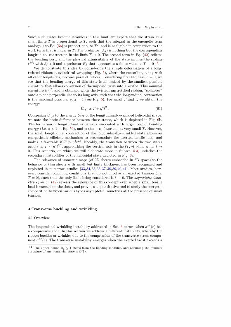
Fig. 8 The parameter plane (T, η) exhibits the helicoid, the far from threshold longitudinalwrinkling and the transverse instability (that is buckling here) when Lt� 1, plotted here fort = 0.005. The coordinates of the triple λ-point are denoted (Tλ, ηλ).
threshold ηtr(T ), whereby the ribbon develops periodic undulations in the trans-verse direction (with wavelength λtr �W ) or a single buckle (λtr ∼W ).
Our analysis highlights two principal differences between the natures of thelongitudinal and transverses instabilities, which are intimately related to the ex-perimental observation in [3]. First, in contrast to the longitudinal threshold, whichoccurs near a curve, ηlon(T ) ≈
√24T , that is independent on the thickness and
length of the ribbon, the threshold ηtr(T ) and the nature of the transverse insta-bility exhibit a strong, nontrivial dependence on t and L. Second, in contrast tothe longitudinal instability, which emerges as a primary instability of the helicoidalstate, the transverse instability underlies two qualitatively distinct phenomena: aprimary instability of the helicoid in a “large” tension regime15 (T > Tλ), wherethe longitudinal stress is purely tensile and a secondary instability of the helicoidpreceded by the longitudinal instability at a low tension regime (T < Tλ). HereTλ is the tension at the λ-point in Fig. 8.
This scenario implies that the tension-twist parameter space (T, η) consists ofthree major phases: A helicoidal state, a FT-longitudinally-wrinkled state, and astate delimited from below by the transverse instability. This division is shown inFig. 8 and strongly resembles the experimental phase diagram reported in [3]. In[3], the instability of the longitudinally-wrinkled state upon increasing twist wasattributed to a “looping” mechanism and was described as a new, third type ofinstability, separate from the longitudinal and transverse instabilities. In our pic-ture, this instability emerges simply as the transverse instability in the low tensionregime, where it is superimposed on the FT longitudinally wrinkled state. Thisinsight provides a natural explanation to the appearance of the “triple” λ-point(Tλ, ηλ =
√24Tλ
)in the tension-twist plane, where the threshold curve ηlon(T )
divides ηtr(T ) into a low-tension branch and a large-tension branch.
15 We place the word “large” in quotation marks to emphasize that the tensile strain T inthis regime is actually small: Tλ(t, L)� T � 1, hence it is fully justified to assume a Hookeanresponse.

28 Julien Chopin et al.
Fig. 9 Schematic phase diagram in log-log scale representing the two regimes L2t� 1 (Left)and L2t � 1 (Right) with the corresponding scaling laws for the horizontal coordinate Tλ ofthe λ-point.
We will show that this phenomenology results from two crucial features ofthe transverse stress in the helicoidal state (Eqs. 3-4) and in the longitudinallywrinkled state (Eqs. 49, 55): (a) For small twist η � 1, the transverse stress is muchsmaller than the longitudinal stress, namely σrr ∼ η2σss � σss. (b) In contrastto the longitudinal stress σss(r) that develops compression only for η2 > 24T , thetransverse stress is compressive everywhere in the (T, η) plane.
Beyond this central result, we predict that the ribbon limit (Eq. 1) exhibits aremarkable effect of the the mutual ratios of the thickness, width, and length of theribbon on the λ-point, the threshold curve ηtr(T ), and the wavelength λtr. Thiscomplex phenomenology is depicted in Fig. 9 and is summarized in the followingparagraph:
• The threshold twist ηtr(T ) vanishes as the ribbon’s thickness vanishes, t→ 0.
• The threshold twist ηtr(T ) diverges as T → 0.
• The tension Tλ(t, L), which separates the regimes of low and “large” tension,vanishes in the ribbon limit at a rate that depends in a nontrivial manner on themutual ratios of the length, width, and thickness of the ribbon: If t� L−2 we findthat Tλ ∼ (t/L)2/3, whereas if L−2 � t we find that Tλ ∼ t.• The mutual ratios between the length, width, and thickness in the ribbon
limit, affect also the type of the transverse instability. Specializing for the “large”tension regime, we find that the transverse instability may appear as a singlebuckle or as a periodic array of wrinkles with wavelength λtr that decreases asT−1/4 upon increasing the tension: (a) If L−1 � t, the transverse instabilityappears as a single buckle of the helicoidal state. (b) If L−2 � t � L−1 thetransverse instability appears as a single buckle for T � (Lt)2 and as a wrinklepattern for (Lt)2 � T � 1. (c) If t � L−2, the transverse instability appears asa wrinkle pattern throughout the whole “large” tension regime.
We start by a scaling analysis of the parameter regime that explains the abovescenario. Then we turn to a quantitative linear stability analysis that yields thetransverse buckling threshold, as well as the shape of the buckled state for aninfinitely long ribbon (or, more precisely, L−2 � t). Finally, we address at somedetail the transverse instability of a ribbon with a finite length (t� L−2 � 1).
Roadmap to the morphological instabilities of a stretched twisted ribbon 29
4.2 Scaling analysis
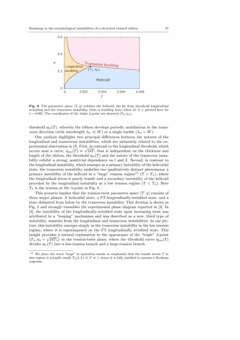
Similarly to the longitudinal wrinkling, the basic mechanism of the transverse in-stability is simply the relaxation of compression (which is now σrr), by appropriatedeformation of the helicoidal shape. Taking a similar approach to Sec. 3, we canfind the scaling relations for the threshold ηtr and the wavelength λtr by identify-ing the dominant destabilizing and stabilizing normal forces associated with suchshape deformation.
The transverse compression gives rise to a destabilizing force ∼ σrr/λ2tr. Thenormal restoring forces are similar to the respective forces that underlie the wrin-kling of a stretched (untwisted) ribbon [8]: bending resistance to deformation inthe transverse direction (∼ B/λ4tr), and tension-induced stiffness due to the spatialvariation of the deformation in the longitudinal direction (∼ T/L2) 16. The bal-ance between these dominant restoring forces and the destabilizing normal forcedue to the compression σrr may lead to buckling, namely λtr ∼ W = 1, if theribbon is extremely long (t � L−1), in which case the tension-induced stiffnessis negligible, or to wrinkling (λtr � W ), where the bending and tension-inducedforces are comparable.
In the following paragraphs we address first the case of an extremely longribbon, where the only dominant restoring force is associated with bending, andthen show how a finite value of L affects a transition from buckling to wrinkling.In each case we will discuss separately the regimes of low and “large” tension, andderive the scaling relation for the λ-point (Tλ, ηλ) that separates these regimes.
Extremely long ribbon: In this case, the tension-induced stiffness is negligible, andthe only significant restoring force to shape deformations is the bending resistance.The transverse instability is then similar to the Euler buckling of a beam of widthW and thickness t, and the instability mode is consequently buckling, i.e. λtr ∼W .The instability threshold ηtr(T ) is obtained when the destablizing force becomescomparable to the stabilizing bending force, namely:
σrr
W 2∼ B
W 4. (62)
The transverse compression σrr(r) is given by Eq. (4) in the helicoidal state (forη2 < 24T ), and by Eq. (55) in the FT longitudinally wrinkled state (for η2 > 24T ).Considering the asymptotic regimes T � η2 in Eq. (4) and T � η2 in Eq. (55),we see that in both “large” and low tension regimes, the transverse stress scalessimilarly with η and T :
σrr ∼ η2T. (63)
Substituting Eq. (63) in Eq. (62), we obtain the scaling of the instability thresholdηtr(T ) for an extremely long ribbon:
ηtr(T ) ∼ t√T. (64)
This scaling relation (with different numerical prefactors in the limits T � Tλand Tλ � T � 1), is confirmed by our detailed calculations in Subsec. 4.3, that
16 All other normal restoring forces, in particular the bending resistance to deformation inthe longitudinal direction that scales as ∼ B/L4 are negligible with respect to these two forces.

30 Julien Chopin et al.
are shown in Fig. 8. The relation (64) demonstrates the singular nature of thetransverse instability: the threshold decreases vanishes with the ribbon’s thickness(t→ 0) and diverges as the exerted tension vanishes (T → 0).
The tension Tλ is the horizontal coordinate of the “triple” λ-point in thetension-twist parameter plane (Fig. 8) at which the transverse buckling changesits character from a primary instability at “large” tension to a secondary insta-bility of the helicoidal state at low tension, which is preceded by the longitudinalwrinkling instability. We find Tλ from Eq. (64) and the relation ηlon(T ) ∼
√T :
Tλ ∼ t . (65)
Ribbon of finite length: Let us assume now that both tension-induced stiffness andbending resistance are significant restoring forces, which balance the destabilizingforce due to transverse compression. The instability onset condition (62) is thenreplaced by
σrr
λ2tr∼ B
λ4tr∼ σss
L2. (66)
Using the scaling law (63) for σrr and estimating σss ∼ T , we obtain the followingscaling relations for the threshold and wavelength:
ηtr ∼√t
LT−1/4, (67)
λtr ∼√LtT−1/4. (68)
In a similar way to the above paragraph, we find the coordinate Tλ of theλ-point by equating Eq. (67) with the relation ηlon(T ) ∼
√T , yielding:
Tλ ∼(t
L
)2/3
. (69)
From buckling to wrinkling: Realizing the important effect of the ribbon’s lengthon the nature of the transverse instability, a natural question is: How long musta ribbon be such that the tension-induced stiffness becomes negligible and thescaling relations (64,65) are valid?
A key to address this question is the obvious inequality λtr ≤W . Substitutingthe scaling relation (69) for Tλ in Eq. (67), and requiring λtr � W , we find thatTλ is characterized by the scaling relation (69) if t � L−2, and by the relation(65) if L−2 � t. This nontrivial dependence of Tλ on the thickness and lengthof the ribbon is depicted in Fig. 9. The behavior of Tλ indicates the nontrivialnature of the ribbon limit, but a closer inspection of Eq. (67), subjected to thecondition λtr ≤W , reveals an even higher level of complexity. Focusing on the largetension regime Tλ < T < 1, and recalling that λtr ≤ W , we find that the ribbonlimit is divided into three sub-regimes that exhibit qualitatively distinct types oftransverse instabilities. This behavior is depicted in Fig. 9, and summarized below:
(a) If t � L−2 � 1, then Tλ satisfies the scaling relation (69) and the trans-verse instability appears as wrinkling, where the threshold ηtr and the wavelengthλtr satisfy the scaling relations (67).
(b) If L−2 � t� L−1 � 1, then Tλ satisfies the scaling relation (65), but thelarge tension regime splits into two parts. For sufficiently small T , the transverse

Roadmap to the morphological instabilities of a stretched twisted ribbon 31
instability appears as a buckling mode (λtr ∼ W ), and the threshold ηtr satisfiesthe scaling (64); for larger values of T (which are nevertheless� 1), the instabilityappears as a wrinkling mode, described by the scaling relations (67).
(c) Finally, if L−1 � t� 1, then Tλ satisfies the scaling relation (65), and thetransverse instability appears as a buckling mode, with the scaling (64), through-out the whole regime of large tension.
4.3 Linear stability analysis
In this subsection we present in detail the linear stability analysis for the case ofan extremely long ribbon, assuming that the ribbon’s shape close to the transverseinstability is well approximated by the form:
X(s, r) =
(1− χ)s+ ζηus1(r)[r + ur(r)] cos(ηs)− ζz1(r) sin(ηs)[r + ur(r)] sin(ηs) + ζz1(r) cos(ηs)
, (70)
where the perturbation’s amplitude ζ is assumed to be infinitesimal, and the func-tions us1(r) and z1(r) correspond to the two degrees of freedom that characterizethe perturbed shape and strain. More precisely, it is reasonable to assume thatthe boundary conditions at the short edges (s = ±L/2) have a prominent effectonly at a zone of size W = 1 near those edges, and barely disturb the transla-tional symmetry of the reference state in the longitudinal direction17. Therefore,the eigenmodes of the system are approximated by:[
usj(r) cos
(πjs+ γj
L
), zj(r) cos
(πjs
L
)](71)
where 1 ≤ j � L. Since we address here an instability that relaxes the transversecompression, the variation in the longitudinal direction should be minimal to avoidany energetic costs, and hence we assume that the first eigenmode to become un-stable is j = 1 (see also [8]). In the next subsection we present an approximateanalysis of the j = 1 mode, but here we simplify further by neglecting the longi-tudinal variation altogether (i.e. replacing cos(πjs/L) → 1). Since all derivativeswith respect to the variable s come with negative powers of L, we anticipate thatthis approximation is valid for sufficiently large L (such that L−2 � t, as foundin Subsec. 4.2).
Our linear stability analysis follows a classical approach, whose first use inelasticity theory has been attributed to Michell [42,43] 18. First, we assume a smallperturbation of the form (70) to the reference state, and expand the generalizedFvK equations (27-28) to linear order in the amplitude ζ, obtaining a set of linearhomogeneous equations. In general, these equations have no solution but the trivialone, us1(r) = z1(r) = 0. For a given tension T , the transverse instability occursat the lowest value ηtr(T ) of the twist for which the buckling equations admit anontrivial solution. This solution is identified as the unstable transverse mode.
17 We will comment on this assumption later in Sec. 6.18 The introduction of [44] contains a useful summary of the various approaches for linear
stability analysis of elastic systems.

32 Julien Chopin et al.
We must compute the perturbed curvature and stress tensors that enter thegeneralized FvK equations (27-28) upon substituting the shape (70), and retainingonly the terms that are linear in ζ. We will limit our analysis to the simple case ν =0. Since the stress field (3-4) has been shown to be independent of the Poisson ratio,we expect that the same is true for the transverse instability.19 The perturbed
curvature tensor is given by cαβ = c(0)αβ + ζc
(1)αβ +O(ζ2), where
c(0)αβ =
(0 ηη 0
), (72)
c(1)αβ =
(−η2
[z1(r)− rz′1(r)
]0
0 z′′1 (r)
), (73)
and the perturbed stress tensor is given by σαβ = σαβ(0) + ζσαβ(1) +O(ζ2), where
σαβ(0) =
(T + η2
2
(r2 − 1
12
)0
0 η2
2
(r2 − 1
4
) [T + η2
4
(r2 + 1
12
)]) , (74)
σαβ(1) =η
2
[u′s1(r)− z1(r) + rz′1(r)
](0 11 0
). (75)
Notice that, to O(ζ), the diagonal stress components are not perturbed. Further-more, the force balance in the transverse direction (28), which we evaluate as usualto O(η4), yields the equations:
0 =η
2
[u′′s1(r) + rz′′1 (r)
], (76)
0 =η3
2
(u′s1(r)− z1(r) + rz′1(r) + 2r
[u′′s1(r) + rz′′1 (r)
]). (77)
These equations are solved by:
u′s1(r) = z1(r)− rz′1(r) (78)
implying that the stress tensor does not deviate from its value at the referencestate.
Turning now to the normal force balance, we substitute Eqs. (73,75,78) inEq. (27), retain the linear order in the amplitude ζ, and obtain a 4th order differ-ential equation for z1(r):
t2
12z(4)1 (r) = −η2σss(0)
[z1(r)− rz′1(r)
]+ σrr(0)z
′′1 (r). (79)
We recognize this equation as similar to the Euler buckling equation, whereby adestabilizing force σrr(0)z
′′1 (r) that originates from the relaxation of compression by
deflection is balanced by the stabilizing bending force t2
12z(4)1 (r) that opposes any
deflection. However, Eq. (79) carries some differences from the simple Euler buck-ling instability. First, the compression σrr(0)(r) is not uniform across the ribbon’swidth. Second, we note the existence of another normal force, that is proportionalto the longitudinal stress σss(0), and originates from the fact that the reference state
19 We just note that a non zero Poisson ratio would require another degree of freedom in theperturbative analysis, namely a transverse in-plane displacement ζur1(r).

Roadmap to the morphological instabilities of a stretched twisted ribbon 33
is non-planar. Since we found that σrr(0) ∼ −η2σss(0) (see Eq. (33)) we can view the
right hand side of Eq. (79) as a renormalized version of the normal force σrr(0)z′′1 (r)
that couples the compression to the curvature. We are poised to solve this equationsubjected to the homogenous boundary conditions:
z′′1 (±1/2) = 0, (80)
z(3)1 (±1/2) = 0. (81)
It is noteworthy that the buckling equation (79) is general and does not dependon the particular form (74) of the stress of the reference state. As a consequence,the linear stability analysis can be performed over the helicoidal state, where thestress is given by Eqs. (3-4), as well as over the FT-longitudinally-wrinkled state,where it is given by Eqs. (49,55)20. The stress field that we have to use dependson our position in the tension-twist plane (T, η) with respect to the longitudinalinstability line η2 = 24T .
Before turning to numerical analysis, it is useful to consider the limit T � η2
(α→∞ in the terminology of Sec. 3), where an analytic solution of the bucklingequations (79-81) is available. In this limit, the exerted tension is supported bytwo narrow strips near the long edges of the ribbon, and the stress field (49,55)becomes:
σss(r) =T
2
[δ
(r +
1
2
)+ δ
(r − 1
2
)], (82)
σrr(r) = −η2T
4, (83)
where δ(r) is the Dirac-delta function. Since the term −η2σss(0)[z1(r)− rz′1(r)
]is
non-zero only at an infinitesimal strip near r = ±1/2, we can eliminate it from(79) by modifying the boundary condition (81) that becomes:
t2
12z(3)1 (−1/2) = −η
2T
2
[z1(−1/2) +
1
2z′1(−1/2)
], (84)
with an analogous condition at the other edge, r = 1/2. The buckling equation (79)now simply reads
z(4)1 (r) = −3η2T
t2z′′1 (r) , (85)
which is the familiar Euler buckling equation under uniform compression. It admitsa non-zero solution z1(r) = cos(πr) when η reaches its threshold value
small T : ηtr(T ) =π√3
t√T. (86)
20 Recall that for a given (η, T ) in the regime η2/T > 24, the FT approach in Subsec. 3.3provides a longitudinally-wrinkled state whose shape is close to the helicoid, up to deviationswhose amplitude vanishes as t → 0, and whose stress is given by (49,55), up to correctionthat also vanish as t→ 0. Therefore, the transverse linear stability analysis in this regime pro-vides expressions for the threshold ηtr(T ) and the unstable mode [us1(r), z1[(r)] that becomeaccurate as t→ 0.

34 Julien Chopin et al.
−1
−0.5
0
0.5
1
−0.5 0 0.5
z 1(r)
r
0.0001
0.001
0.01
T
Fig. 10 Shape of the transverse unstable mode in the limit of an infinitely long ribbon (L→∞) of thickness t = 0.005, as a function of the exerted tension. For the range of tension appliedhere, the limit L→∞ is relevant for lengths L > 20 (see Eq. 68).
In the opposite limit, T � η2, an analytic solution of Eq. (79) is not available anda numerical solution of Eqs. (79-81) yields the threshold in this limit:
large T : ηtr(T ) = 4.4t√T. (87)
Interestingly, the two asymptotic expressions (86,87) exhibit the scaling law (64),not only with the ribbon’s thickness t, but also with the tension T .
Our numerical results and the subsequent division of the tension-twist planeinto three major phases (the helicoid, the longitudinal wrinkling and the regionabove the transverse instability) are shown in Fig. 8 for the thickness t = 0.005.This phase diagram exhibits a striking similarity, at a quantitative level, with thephase diagram found experimentally in [3] for the same thickness.21
The numerical analysis of the buckling equation gives also the shape of thebuckling mode, which we show in Fig. 10 for a few representative values of T .Choosing some (arbitray) small amplitude, we draw the shape of the buckledribbon in Fig. 11.
4.4 Effect of a finite length
Our analysis in this paper assumes that the ribbon is long, such that the effect ofboundary conditions at s = ±L/2 is limited to the vicinity of the short edges, andthe linear eigenmodes can be expressed through a Fourier series, Eq. (71), wherethe most unstable one is j = 1. In Subsec. 4.3 we went beyond this assumption andneglected the spatial variation of this unstable mode in the longitudinal direction,expecting it to make a negligible contribution to the force balance if L is sufficiently
21 The experimental value of the length in [3] is L = 20. The maximal tension in the exper-iment is Tmax = 0.01; from Eq. (68), we deduce that the minimal transverse wavelength is
λmin ∼√LtT
−1/4max = 1. This explains why buckling is observed and why the infinite length
approximation is in good agreement with the experiment.

Roadmap to the morphological instabilities of a stretched twisted ribbon 35
Fig. 11 Shape of the ribbon undergoing a transverse instability: (a) single mode buckling ofa very long ribbon (b) wrinkling of a ribbon with Lt� 1.
large. In this subsection we relax this last assumption, by taking into considerationthe longitudinal variation of the perturbation. This mean that the ribbon is notsufficiently long to justify a complete neglecting of the spatial variation, but it islong enough such that the mode structure is given by Eq. (71, j = 1). 22
Despite its simple form, a complete analysis of the mode j = 1 in Eq. (71)is rather cumbersome. In order to simplify our calculation we will retain onlythe term in the normal force balance that couples the longitudinal stress and thelongitudinal curvature. Such a term was found to be crucial for the wrinkling of astretched, untwisted sheet [8]. We thus obtain the buckling equation
t2
12z(4)1 (r) = −η2σss(0)
[z1(r)− rz′1(r)
]+ κ2σss(0)z1(r) + σrr(0)z
′′1 (r), (88)
where κ = π/L, subjected to the same boundary conditions that we described inthe previous subsection.
The buckling equation can be solved numerically, and the effect of the finiteribbon length on the phase diagram is shown on Fig. 12. The main effect of thefinite length is to increase the transverse buckling threshold; this is expected, sincethe new term is a stabilizing term. We also note that this effect is not importantat small tension. Another effect is that the threshold ηtr(T ) may become a non-monotonic function, due to the fact that the tension enhances both the compressive(destabilizing) term and the stretching (stabilizing) term, which are represented,respectively, by the third and second terms of Eq. (88).
Finally, as was noted already in our scaling analysis, the unstable transversemode transforms from buckling to wrinkling as the tension increases. This trans-formation is shown in Fig. 13.
22 If the ribbon becomes even shorter, it is possible that the boundary effect is sufficientlystrong and the assumed mode structure Eq. (71) is not valid. In Sec. 6 we discuss the possibilitythat this might happen even in the ribbon limit (i.e. L� 1) provided t is small enough.

36 Julien Chopin et al.
Fig. 12 Effect of a finite ribbon length on the phase diagram: for a thickness t = 5×10⁻⁴, thetransverse buckling threshold is plotted for L = ∞ (dashed line) and L = 10 (solid line). Forthis thickness and this tension range, the infinite length approximation is relevant for lengths
such that L > t−1T1/2max ' 100 (from the requirement that λ > 1 in Eq. (68)).
0
1
−0.5 0 0.5
z 1(r)
r
0.0001
0.001
0.01
T
−1
0
1
−0.5 0 0.5
z 1(r)
r
0
20
40
60
80
L
Fig. 13 Transition from transverse buckling to transverse wrinkling as a function of thetension and length. Shape of the transverse unstable modes: Left : t = 5 · 10−4, L = 10 andtensions T = 10−4, 10−3 and 10−2. Right : t = 0.0005, T = 0.01 and ribbon lengths L = 5, 35and 80.
5 Twisting with little tension, stretching with little twist
5.1 Overview
In Secs. 2-4 we assumed that the shape of the stretched-twisted ribbon is close toa helicoid, and employed asymptotic methods to characterize the deviations fromthis shape. This approach allowed us to compute the curves ηlon(T ) and ηtr(T ) thatunderlie the division of the (T, η) plane into three major regimes (Fig. 3), and tocharacterize the helicoidal state (blue), the longitudinally wrinkled state (orange),and the margins of the third regime (pink), close to the transverse instabilitythreshold. The proximity to a helocidal shape is violated at the bulk of the pinkregime, which we do not address in this paper, where the self-contact zones emergeand the helicoidal shape is greatly mutilated [3]. Other two parameter regimeswhere the ribbon’s shape may become very different from a helicoid are the edge

Roadmap to the morphological instabilities of a stretched twisted ribbon 37
of the blue regime (i.e. close to the horizontal line η = 0), where the ribbon isstretched with little twisting, and the edge of the orange regime (i.e. close to thevertical line T = 0), where the ribbon is twisted with little tensile load. In thissection we discuss the expected transformations to non-helicoidal morphologiesin these parameter regimes: a nearly planar shape as η → 0, where the twist isabsorbed in the vicinity of the short edges; and the formation of a creased helicoidalshape and cylindrical wrapping as T → 0.
In contrast to previous sections (2-4), where we carried out a rigorous studybased on the helicoidal solution to the cFvK equations, its linear stability anal-ysis, and an FT analysis, our discussion in this section is more heuristic, and isbased on energetic estimates and scaling arguments. We start in Subsec. 5.2 witha general discussion of the difference between plate-like and rod-like approaches tothe mechanics of ribbons. The first approach, which we employed in previous sec-tions, is based on the cFvK equations; the second approach consists of Kirchoff’srod equations or Sadowsky equation, the last one provides the mathematical ba-sis for a theoretical description of the creased helicoidal state [7]. We take thisopportunity to explain why the Kirchoff’s rod equations cannot be used to studythe ribbon limit (Eq. 1). In Subsec. 5.3 we briefly describe the work of [7] on thecreased helicoidal state, and explain how it gives rise to another type of asymp-totic isometry, different from the longitudinally-wrinkled helicoidal shape and thecylindrical wrapping state. In Subsec. 5.4 we turn to the vicinity of the horizontalline η = 0, and introduce an energetic comparison that allows us to estimate theminimal twist necessary to developing a helicoidal shape for a long ribbon (L� 1)subjected to tension T and clamping of its short edges.
5.2 Theory of elastic ribbons: plate-like or rod-like ?
In the plate-like approach, one employs the cFvK equations for elastic plates withHookean material response to find the shape of the ribbon’s midplane X(s, r).Except the restriction to small strains, no further assumptions are made on thedeformation of the cross section or on the stress profile in the transverse directionr. This “transversial freedom” was reflected in our analysis of the cFvK equationsin sections 3-4 through the r-dependence of the stresses and the consequent shapedeformations, which underlie both longitudinal and transverse instabilities of thehelicoidal state. The transversial freedom encapsulates the conceptual differencebetween the plate-like approach and the rod-like approach, wherein the ribbon’sshape is derived from a curve Xcl(s) that characterizes the shape of the center-line. In the Kirchoff’s method, which addresses the ribbon as a rod with highlyanistropic cross section, the ribbon is allowed to have a tensile strain and the crosssection (i.e. the ribbon’s shape in the plane perpendicular to the centerline) isassumed to retain its shape [29]. The relation between the midplane’s shape andthe centerline is simply:
Kirchoff rod : X(s, r) = Xcl(s) + rr(s) , (89)
where r(s) is the normal to the the tangent vector t = dXcl(s)/ds in the ribbon’smidplane. In the Sadowsky’s method, the ribbon is assumed to be strainless, and

38 Julien Chopin et al.
the shape of the midplane is related to the centerline by the following relation:
Sadowsky strip : X(s, r) = Xcl(s) + r
[b(s) +
τ(s)
κ(s)t(s)
], (90)
where b(s) is the Frenet binormal to the curve Xcl(s) and τ(s), κ(s), are its torsionand curvature [7]. Assuming a ribbon at mechanical equilibrium, the two methodsyield strictly different sets of force balance equations that yield the centerlineXcl(s). In the rest of this subsection, we briefly recall recent studies of Kirchoffequations of stretched-twisted rods with anisotropic cross section, and explain whythese analysis do not pertain to the ribbon limit, Eq. (1). In the next subsectionwe review a recent work that employed the Sadowsky strip to describe the creasedhelicoidal state of a stretched twisted ribbon, and discuss the regime in the (T, η)plane describable by this method.
Anisotropic Kirchoff’s rod: The instability of a rod with circular cross sectionthat is subjected to tension and twist, and the consequent formation of loops,has been studied already by Love [45], using the Kirchoff’s rod equations. Thetheoretical works of Champneys, Thompson and van der Heijden [10,11,12] andof Goriely et al. [9], employed the Kirchoff’s rod equations to study the responseto tension and twist of a rod with asymmetric (i.e. non-circular) cross section. Animportant finding of these studies was the existence of instabilities (termed “thick”and“tapelike” [9]), through which the straight centerline that defines a helicoidalstate of the ribbon becomes unstable (see Fig. 3 of [9]). The visual similarity ofthe “thick” mode to the secondary instability of a stretched-twisted ribbon at lowtension (which we described in Sec. 4 as a transverse instability superimposedon the longitudinally wrinkled ribbon), motivated the original portraying of thatinstability as “looping” [3].
However, a close inspection of the phase diagram of [3] (Fig. 3), shows nosigns of the instability predicted by [10,11,12]. Translating the results of [9] toour notations (see Appendix B) and considering the ribbon limit (a � 1 in theterminology of [9]), we find that the theoretical prediction suggests an instability ofthe helicoidal state around the curve η ≈
√cT with 1/2 < c < 2.8, at which range
of parameters the experiments of [3] show a stable helicoidal state. This observationindicates that using the Kirchoff’s rod equation may not be suitable at the ribbonlimit (Eq. 1), where the cross section is highly anisotropic. Indeed, the Kirchoff’sequations assume fixed values of the torsion and bending modulii (i.e. independenton the exerted loads), which characterize the response of unstretched, untwistedribbon to infinitesimal loads. As was noted by Green, who considered the twistedribbon as a 3D solid body, this assumption becomes invalid if the exerted twistη � t (see Eq. (21) of [1]). As a consequence, the Kirchoff’s rod equation cannotbe used to describe the helicoidal state of a twisted ribbon without appropriaterenormalization of the rod’s modulli (that reflect the exerted twist and possiblyalso the tensile load).
5.3 The creased helicoidal state: a second look at asymptotic isometries
The shape of a perfectly inextensible ribbon (Eq. 90), has been addressed by Korteet al. [7], who built upon earlier studies [6,46,26]. These authors found that under
Roadmap to the morphological instabilities of a stretched twisted ribbon 39
given twist η and a range of tensile loads, the ribbon admits a strainless state,whose morphology is similar to the creased helocid state found in the experimentsof [3]. In fact, the theory of [7] yields a family of such states, parametrized by theangle between triangular facets. Importantly, the construction of [7] consists of“true” creases, with infinitely large curvature, whose bending energy would havebeen infinite if the ribbon had any thickness. The underlying assumption in [7]is that at a small, finite thickness, these creases are slightly smoothed (i.e. thecurvature diverges as t → 0 at a narrow zone whose size vanishes at the samelimit), such that the overall bending energy of the crease vanishes as t → 0.Such a “stress focusing” mechanism has been instrumental in studies of crumpledsheets [34].
In order to identify the regime in the (T, η) plane in which the ribbon’s mor-phology is describable by this approach we must clarify the meaning of “tensileload” on a purely inextensible (i.e. strainless) ribbon. For this purpose, we willuse in this paragraph dimensionfull parameters (denoted by non-italicized fonts),introducing explicitly the ribbon’s width W and stretching modulus Y, which aretaken to define, respectively, the units of length and stress throughout this paper.The dimensionfull bending modulus is B ∼ YW2t2. (Recall that we defined t,Eq. (1) as the ratio between the ribbon’s thickness and its width). A thin elasticribbon of width W has two characteristic scales for stress exerted on the midplane(i.e. force/length): The first one is just the stretching modulus Y, which is theproduct of the Young’s modulus of the material (E) and the ribbon’s thickness(tW); the second scale for stress is related to the bending modulus B/W2 ∼ Yt2.Since both scales are proportional to the Young’s modulus E, it is impossible to as-sume a “prefectly inextensible” ribbon (i.e. Y =∞) that is nevertheless bendable(i.e. B < ∞). Hence, attributing an “inextensibility” feature to an elastic ribbonmust be understood as assuming the asymptotic limit t→ 0, such that the exertedtensile load vanishes in comparison to Y but not in comparison to B/W2 = Yt2.Returning to the parameter plane (T, η), we may expect that for a given twist η,the family of creased helicoid states predicted by [7] exists at a parameter regimeC1t
2 < T < C2t2 (where C1,2 depend on η). In this regime, the exerted tension is
sufficiently small with respect to the stress scale set by the stretching modulus Y,such that the state of the ribbon is nearly strainless and is thus close to an isom-etry of the untwisted ribbon; at the same time, the tension is sufficiently large incomparison to the other stress scale set by the bending modulus and the ribbon’swidth, Yt2, such that the necessary conditions for constructing a creased helicoidstate by the method of [7] are satisfied.
The creased helicoid state as an asymptotic isometry: The above paragraph indi-cates that the analysis of [7] addresses the stretched, twisted ribbon, in the vicinityof the hyper-plane (T = 0, t = 0) in the 4D parameter space spanned by the di-mensionless parameters t, L, T and η (Eq. (1)). As we argued in Subsec. 3.5, theribbon mechanics in this regime reflects a competition between distinct types ofasymptotic isometries – states whose elastic energy at a small neighborhood ofthat singular hyper-plane is described by Eq. (42). The creased helicoid of [7] isyet another example of an asymptotic isometry, and its energy in that limit canalso be expressed, as a linear function of T : The intercept, T -independent termof the energy (Eq. 42), is governed by the bending energy of the creases at smallfinite t; the term that is linear in T originates from the work done by the tensile

40 Julien Chopin et al.
load, where the prefactor is the t-independent longitudinal contraction χCH of the
ribbon in the creased helicoid state 23.In order to carry out a quantitative comparison between the energies of the
cylindrical wrapping, longitudinal wrinkling, and creased helicoid states, we mustknow the longitudinal contractions (Aj), as well as the exponents (βj) that char-acterize the bending energy of the states at the vicinity of the hyper-plane (T =0, t= 0). While we do not have yet the complete set of those values for all threetypes of asymptotic isometries, the schematic plot in the inset of Fig. 6b seemsas a plausible scenario to us: At a given η, the bending energy of the cylindricalwrapping (i.e. the intercept of the the linear function in Fig. 6b) is minimal, andtherefore this state should be observed if the exerted tension T is very small; uponincreasing T , the experimental observations of [3] indicate that a creased helicoidstate is formed and then gives way to a longitudinally wrinkled state, suggest-ing that creased helicoids are characterized by lower bending energy and largerlongitudinal contraction in comparison to the longitudinal wrinkles.
5.4 Helicoid versus planar state: from boundary-dominated to twist-dominated
So far, we assumed that the highly-symmetric state of a stretched-twisted ribbon,characterized by translational symmetry along the longitudinal direction s, is thehelicoid. We carried out stability analysis of the helicoidal state and studied thetransitions to states that break its translational symmetry. However, if the ribbonis sufficiently long (L� 1) and the exerted twist η is sufficiently small with respectto T , one may envision that the unbuckled state of the ribbon is not a helicoidbut rather a stretched, planar ribbon, where the exerted twist remains confinedto the vicinity of the short edges (see Fig. 14). Such a localized-twist state canbe described as a perturbation to the well-known problem of purely stretchingan elongated ribbon, where 0 < T � 1 and η = 0 [8]. For that problem, it wasfound that the clamping of the short edges together with the Poisson ratio effectgives rise to contraction of the ribbon in the transverse direction not only in thevicinity of the clamped edges, but rather throughout most of the ribbon’s length(see [8]). Recalling our discussion in previous sections, one may conclude thatthere exist two distinct causes for transverse buckling and wrinkling in a ribbon:The first one, which we described above (Sec. 4), is a “bulk” mechanism, whereσrr becomes compressive due to the simultaneous effect of uniaxial stretchingalong s and uniform twist η, experienced by any piece of the ribbon. The secondmechanism is essentially a boundary-generated effect, whereby the tendency of theribbon to transverse contraction (ur(1/2) = −νT/2 in Eq. (29)) away from theclamped edges gives rise to a small transverse compression σrr < 0, which is alsorelieved by wrinkles. A natural question is whether, for a given set of parametersthe emergence of a compressive transverse stress σrr and the consequent buck-ling/wrinkling instability, are governed by the bulk effect (twist) or rather by theboundary effect (clamping).
In order to address this question, we have to compare the compressive stresses(σrr < 0) associated with twist and with clamping of the short edges. However,
23 More precisely, the contraction χCH
, as well as the bending energy of the crease may
depend on the angle between triangular facets, and hence the analysis of [7] leads to a familyof asymptotic isometries parameterized by that angle.

Roadmap to the morphological instabilities of a stretched twisted ribbon 41
Fig. 14 Picture of the ribbon’s shape at very small twist, (a) Helicoidal state, given forcomparison with (b) Boundary dominated state where the twist is confined in the vicinity ofthe short edges, the central part being flat.
while the first one was derived above (Eq. 4), we are not aware of a similar analyticexpression for the transverse stress due to clamped edges 24. Hence, we will proceedby estimating the relevant energies. We will do this by denoting U0 = T 2 theenergy per length of a stretched ribbon that is not clamped and not twisted,and estimating the excess energies associated with twist and clamping, which wedenote, respectively, by ∆Utwist and ∆Uclamp. Our purpose is to find the curveη∗(T ) in the (T, η) plane, below which the clamped-edge effect is significant.
The excess energy ∆Utwist: Expecting the transition from twist-dominated toclamping-dominated instability to occur at a small value of η, we neglect terms oforder O(η4) in comparison to terms of order O(η2T ), and thus estimate ∆Utwist
by considering a stretched, twisted, unclamped ribbon:
∆Utwist ≈∫ 1/2
−1/2
εss(r)2dr − U0 ∼ Tη2 , (91)
where we considered only the leading order in η2, and therefore neglected theenergy due to the strain ε2rr.
The excess energy ∆Uclamp: Consider now a stretched, clamped, untwisted ribbon.In Appendix C we show that the deviation of the longitudinal strain εss fromthe “base” value T is proportional to the Poisson ratio ν and is restricted todistances ∼ 1 from the clamped edges, at which zone the transverse and shearstrain components also have nonvanishing values that are proportional to ν. Thisallows us to estimate:
∆Uclamp ∼νF (ν)T 2
L, (92)
where F (ν) is some smooth function of ν that satisfies F (ν)→ cst for ν → 0.
24 The well-known work of Cerda and Mahadevan [8] addressed this problem in the far-from-threshold regime, where wrinkles are fully developed and the transverse compression cannotbe approximated by its value at threshold. The planar (unbuckled) state that underlies thewrinkling instability due to clamped boundaries was studied numerically in some recent works[47,48]. However, these works did not address the ribbon limit L � 1 that we study here. Acouple of papers [49] attempted to extend the far-from-threshold approach of [8] to the near-threshold regime (by invoking effective ”inextensibility” constraints), but the justification ofthis approach has yet to be established.

42 Julien Chopin et al.
Comparing now our estimates for the excess energies ∆Utwist and ∆Uclamp, wefind that the transition from the clamping-dominated zone to the twist-dominatedzone is expected to occur around:
η∗ ∼√νT
L, (93)
confirming our expectation that η∗(T ) approaches the T axis for small Poissonratio and large L. For η < η∗, we expect that a transverse buckling instability istriggered by the clamped boundaries, whereas for η > η∗ we expect the instabilitymechanism described in the previous sections.
We have to compare the above expression with the threshold for the transverseinstability found in Sec. 4, ηtr ∼
√tT−1/4. We find that both values are comparable
when
T = Tclamp ∼(Lt
ν
)2/3
, (94)
the effect of clamping on the transverse instability cannot be neglected if the ten-sion is sufficiently large, T > Tclamp
25. Above this critical tension, the transverseinstability is governed by the clamped boundaries rather than the helicoid geom-etry.
6 Discussion
Our theoretical study identified distinct types of morphologies in different regimesof the 4D parameter space spanned by T, η, t and L−1. These dimensionless pa-rameters are assumed small (Eqs. 1, 2), and one may be tempted to describethe ribbon as “thin” (t � 1), “long” (L−1 � 1), subjected to “small” tensileload (T � 1), and “slightly” twisted (η � 1). However, our analysis highlightsthe deceptive nature of such a colloquial description, since the ribbon exhibitsmarkedly different behaviors in different “corners” of the 4D parameter space.In other words, the relevant parameters that govern the ribbon’s morphology arevarious ratios between the four control parameters T, η, t and L rather than the“bare” value of each control parameter. The challenge for an experimenter, whomay be motivated by the predictions in this paper, is to construct a set-up thatallows access to those distinct regimes and precise measurements of observablesthe characterize the transitions between them. In this section we will focus on thisexperimental perspective, propose specific measurements, and describe a few openquestions that await further theoretical and experimental study.
25 If L ∼ 1, as was the case in Fig. 3 of [3], this equation means that the transverse wrinklingreflects the clamping mechanism of the Cerda and Mahadevan stretched sheet [8] rather thanthe helicoidal mechanism described in Sec. 4.

Roadmap to the morphological instabilities of a stretched twisted ribbon 43
Fig. 15 Ranges of tension and length probed by the experiments [3,2]. (a) Tension: theGreen’s plateau for ηlon(T ) pictured in Fig. 3c is expected for T � Tsm, longitudinal wrin-kling (near threshold and far from threshold) is expected for Tsm < T < Tλ, and transversebuckling/wrinkling becomes a primary instability of the helicoid for T > Tλ. The upper limitTHook is the limit of linear Hookean response of the material. (b) Length: (in depicting this
figure we assume Lclamp = νt−1T 3/2 � t−1/2, see Eq. (94)). For lengths L > t−1 the primarytransverse instability is buckling; For L < Lclamp the transverse instability is governed by the
clamping of the short edges, similarly to [8]; For Lclamp � L� t−1/2, the transverse instabil-
ity is wrinkling; finally for lengths in the range t−1/2 � L� t−1 we predict a crossover frombuckling to wrinkling as the exerted tension T varies from Tλ to THook (see Fig. 13(Left)).
6.1 Experimental considerations
6.1.1 Objectives
Let us assume a ribbon with a fixed thickness and width, such that the parametert is fixed at a very small value (say, t ≈ 10−5), and address the desired range ofthe other control parameters.
• Controlling T : As Fig. 15a depicts, the tension T may vary between Tmin,which is determined by the quality of the set-up, and THook � 1, above whichthe material response can no longer be approximated through Hookean elasticity.Ideally, one would like Tmin � Tsm(t) and THook � Tλ, where Tsm ∼ t2 (Eq. 46)
and Tλ ∼ max{t, (t/L)2/3
}(Eqs. 65,69). As we describe in the next subsection,
varying the tensile load in the range (Tsm, Tλ) will allow probing most of the phe-nomena associated with the formation and nature of the longitudinally-wrinkledpattern (Subsec. 3.2-3.4), Fig. 3d), and the mechanism by which it becomes unsta-ble at sufficiently low T and given η (Subsec. 5.3, Fig. 3a); varying the tensile loadin the range (Tλ, Tmax) is necessary to understand the effect of T on the transverseinstability (Sec. 4).
• Controlling L: As Fig. 15b depicts, a desired set-up should allow variationof the ribbon’s length L from Lmin to Lmax, where 1 < Lmin � t−1/2 andLmax � t−1. Varying L in such a range will provide an access to most of thepredictions associated with the transverse instability: the wrinkling-buckling tran-sition (Sec. 4.4, Fig. 3b), the scaling law of the triple point (Eqs. 65,69), and thepossible existence of a localized transverse buckling mode even for a very longribbon, which we discuss in the next subsection.
• Controlling η: A good experimental set-up may allow a nearly-continuousvariation of the imposed twist angle θ = ηL. For instance, if θ is varied by incre-ments of 1o then the minimal twist that could be imposed is ηmin ≈ 2π/(360 L).A reliable control on ηmin is required for two purposes: In the very low tensionregime (T < Tsm(t)), it may allow to address Green’s “plateau” of the longitudinal
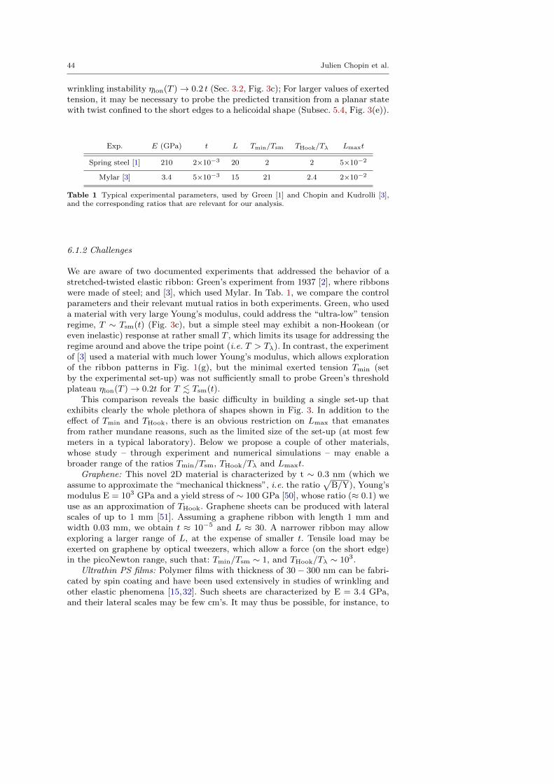
44 Julien Chopin et al.
wrinkling instability ηlon(T )→ 0.2 t (Sec. 3.2, Fig. 3c); For larger values of exertedtension, it may be necessary to probe the predicted transition from a planar statewith twist confined to the short edges to a helicoidal shape (Subsec. 5.4, Fig. 3(e)).
Exp. E (GPa) t L Tmin/Tsm THook/Tλ Lmaxt
Spring steel [1] 210 2×10⁻³ 20 2 2 5×10⁻²
Mylar [3] 3.4 5×10⁻³ 15 21 2.4 2×10⁻²
Table 1 Typical experimental parameters, used by Green [1] and Chopin and Kudrolli [3],and the corresponding ratios that are relevant for our analysis.
6.1.2 Challenges
We are aware of two documented experiments that addressed the behavior of astretched-twisted elastic ribbon: Green’s experiment from 1937 [2], where ribbonswere made of steel; and [3], which used Mylar. In Tab. 1, we compare the controlparameters and their relevant mutual ratios in both experiments. Green, who useda material with very large Young’s modulus, could address the “ultra-low” tensionregime, T ∼ Tsm(t) (Fig. 3c), but a simple steel may exhibit a non-Hookean (oreven inelastic) response at rather small T , which limits its usage for addressing theregime around and above the tripe point (i.e. T > Tλ). In contrast, the experimentof [3] used a material with much lower Young’s modulus, which allows explorationof the ribbon patterns in Fig. 1(g), but the minimal exerted tension Tmin (setby the experimental set-up) was not sufficiently small to probe Green’s thresholdplateau ηlon(T )→ 0.2t for T . Tsm(t).
This comparison reveals the basic difficulty in building a single set-up thatexhibits clearly the whole plethora of shapes shown in Fig. 3. In addition to theeffect of Tmin and THook, there is an obvious restriction on Lmax that emanatesfrom rather mundane reasons, such as the limited size of the set-up (at most fewmeters in a typical laboratory). Below we propose a couple of other materials,whose study – through experiment and numerical simulations – may enable abroader range of the ratios Tmin/Tsm, THook/Tλ and Lmaxt.
Graphene: This novel 2D material is characterized by t ∼ 0.3 nm (which weassume to approximate the “mechanical thickness”, i.e. the ratio
√B/Y), Young’s
modulus E = 103 GPa and a yield stress of ∼ 100 GPa [50], whose ratio (≈ 0.1) weuse as an approximation of THook. Graphene sheets can be produced with lateralscales of up to 1 mm [51]. Assuming a graphene ribbon with length 1 mm andwidth 0.03 mm, we obtain t ≈ 10−5 and L ≈ 30. A narrower ribbon may allowexploring a larger range of L, at the expense of smaller t. Tensile load may beexerted on graphene by optical tweezers, which allow a force (on the short edge)in the picoNewton range, such that: Tmin/Tsm ∼ 1, and THook/Tλ ∼ 103.
Ultrathin PS films: Polymer films with thickness of 30− 300 nm can be fabri-cated by spin coating and have been used extensively in studies of wrinkling andother elastic phenomena [15,32]. Such sheets are characterized by E = 3.4 GPa,and their lateral scales may be few cm’s. It may thus be possible, for instance, to

Roadmap to the morphological instabilities of a stretched twisted ribbon 45
create ultrathin PS ribbons with L ≈ 102 and t ≈ 10−4. Capillary forces have beenused to exert tension on floating ultrathin PS sheets, where the surface tensionvaries from a maximum of ≈ 70 mN/m to 3 times lesser than this value (by usingsurfactants). This corresponds to Tmin/Tsm ∼ 104, THook/Tλ ∼ 20 (for t ≈ 300nm).
Thus, making ribbons from graphene or ultrathin PS films may allow a broadrange of the three most relevant ratios (right columns of Tab. 1) that are necessaryto explore the various asymptotic regimes of the system. We recall though, thatboth graphene and ultrathin polymer sheets are rarely used in a free-standingform, which is the one needed for the stretch-twist experiment that we addresshere.
6.2 Proposed measurements and open questions
Let us now discuss the specific parameter regimes and the corresponding morpho-logical instabilities addressed by our theory. In each of the following paragraphswe will propose measurements and mention open theoretical questions.
6.2.1 Longitudinal wrinkling at Tsm < T < Tλ
The parameter regime Tsm < T < Tλ (Tsm is defined in Eq. 47) was addressed inthe experiment of Chopin and Kudroli [3], who found that the threshold ηlon(T )becomes close to the curve
√24T at which the Green’s stress predicts longitudinal
compression. In this regime, our discussion in Sec. 3 predicts the emergence of theFT regime rather close to the threshold curve.
Experiment: Chopin and Kudroli [3] used ribbons with t = 5 ·10−3 and confirmedthat the threshold ηlon(T ) is close to the curve
√24T , at which the Green’s lon-
gitudinal stress becomes compressive. Additionally, the dependence of ∆αlon andλlon on t and T (Eq. 45) was in excellent agreement with the prediction of the NTapproach [5]. Such a value of t, however, may be too large to probe the transitionfrom the NT to the FT regime predicted in Sec. 3, since the initial width of thewrinkled zone (rwr ∼ λlon) is already a relatively large fraction of the ribbon’swidth. Using thinner ribbons (e.g. t ∼ 10−5) may lead to substantially smallervalue of the initial width of the wrinkled zone, such that the different predictionsof the NT and FT methods for rwr(α) (Fig. 4) may be more pronounced.
A useful probe for testing the predicted NT-FT transition may involve thelongitudinal contraction χ(α) (Eqs. 20, 52, Fig. 5). The function χ(α) may beeasier to measure in comparison to the width rwr(α) of the wrinkled zone, whichrequires the usage of optical tools. Notably, the NT and FT predictions for thelongitudinal contraction are significantly different, wherein the last one becomes3 times smaller than the first for sufficiently large α.
Theory: Our FT analysis in Subsec. 3.3 has been focused on the dominant part ofthe elastic energy of the longitudinally wrinkled state, stored in the asymptotic,compression-free stress field. The dominant energy is associated with macroscalefeatures, which do not depend explicitly on t, and underlies the predictions for rwr
and χFT. However, as we emphasized in Subsec. 3.3, a complete characterization of

46 Julien Chopin et al.
the wrinkle pattern requires evaluation of the subdominant energy, which includesthe bending cost due to wrinkles, as well as the comparable cost due to the forma-tion of a wrinkled structure on the stretched helicoidal shape. The calculation ofthe subdominant energy may involve some subtleties, such as internal boundarylayers [27] and the possible formation of wrinkle cascades rather than a simply pe-riodic structure [28]. Importantly, the actual subdominant mechanics that governthe wrinkle wavelength may depend on the confinement parameter α and there-fore the exponent β that characterizes the subdominant energy (Eq. 59) may takedifferent values in the limit α→ 24 (where the helicoidal shape is highly strained)and the limit α → ∞, at which the longitudinally-wrinkled helicoid becomes anasymptotic isometry of the ribbon. Therefore, evaluation of the subdominant en-ergy is essential not only for finding the fine structure of the wrinkle pattern, butalso to understand how it becomes unstable with respect to the creased helicoidshape as α becomes large (i.e. the limit T → 0 for fixed η).
6.2.2 Longitudinal wrinkling at T < Tsm
Green’s theory [2] consists of a linear stability analysis of the helicoidal state(Eqs. 11,21-22) in the limit T → 0, where the longitudinally buckled/wrinkled zoneis not confined to the vicinity of the centerline, but rather expands throughoutthe whole width of the ribbon. This (NT) analysis yields the threshold plateauηlon(T )→ 0.2 t as T → 0, which was obtained (with deviation of 10%) in Green’sexperiment [2].
Experiment: The experimental data in Green’s paper [2] does show a goodagreement with the theoretical prediction based on his linear stability analysis.However, the available data (figures 4 and 5 of [2]) may not be sufficient to deter-mine whether the actual instability observed by Green was a longitudinal wrinklingor a creased helicoid state. This confusion is illustrated in Fig. 3c, which reflectsour expectation that a creased helicoid pattern (or even a cylindrical wrappingstate) may be observed sufficiently close to the vertical line T = 0. The possibleemergence of a creased helicoid state directly from the helicoidal state (i.e. with-out an intervening wrinkle pattern) may indicate that the longitudinal instabilitychanges its supercritical (continuous) character, becoming a subcritical bifurcationat sufficiently small T . A careful experiment may provide a conclusive answer tothis question.
Theory: The confusing nature of the longitudinal instability at the regime T <Tsm, depicted in Fig. 3c, is reflected also in the fuzziness of the NT-FT transitionin this regime. The FT approach (Subsec. 3.3) assumes that the wrinkle patternnear threshold is confined to a strip of width rwr < 1/2 around the centerline, anddescribes how rwr varies upon increasing the confinement α. However, for T < Tsm,Green’s analysis [2] shows that the ribbon is deformed across its whole width assoon as the longitudinal instability sets in. A natural question is whether the FTregime of the longitudinally wrinkled helicoid terminates at a small T ∼ Tsm.A related question is whether a disappearance of the NT-FT transition below acertain tensile load indicates a qualitative change of the longitudinal instabilityfrom a supercritical to a subcritical type.

Roadmap to the morphological instabilities of a stretched twisted ribbon 47
6.2.3 From longitudinal wrinkling to the creased helicoid state
For a given twist η and sufficiently small tensile load T , we expect the formation ofa creased helicoid state (Fig. 3), predicted in [7] and observed in [3]. Our energeticargument, based on the asymptotic isometry equation, Eq. (42), suggests the exis-tence of a transition between the creased helicoid state and the FT-longitudinally-wrinkled state, which becomes sharply localized along a curve in the parameterplane (T, η) in the limit t→ 0, as is illustrated in Fig. 3a.
Experiment: Chopin and Kudroli [3] did observe such a transition, but notedthat “ ... the longitudinally buckled ribbon evolves continuously into a self-creasedhelicoid ... ”. The appearance of a smooth crossover, rather than a sharp transitionbetween these states, could be attributed to the thickness parameter used in theirexperiment (t ≈ 5 · 10−3), which may be sufficiently small to notice the “wake”of a morphological phase transition that becomes asymptotically sharp as t → 0,but not the acute, critical nature of the transition. Future experiments may haveto use significantly smaller values of t in order to study this transition.
A useful indirect probe of the transition from a longitudinal wrinkling to acreased helicoid state may again be the longitudinal contraction of the ribbonχ(T, η). The FT approach (Subsec. 3.3) predicts the T -dependence through thefunction χFT(α) (Fig. 5) and we expect that the method of [7] yields anotherfunction χCH(T, η). A signature of a sharp morphological transition between thetwo states may be a discontinuity of the measured derivative (∂χ/∂T )η at a curveTc(η) in the (T, η) plane.
Theory: As we pointed out in Subsec. 5.3, our schematic plot of the energies ofthe longitudinal wrinkling and the creased helicoid states (Fig. 6b) reflects theirasymptotic isometry in the vicinity of the hyper-plane (T = 0, t = 0), but has aheuristic content, since the coefficients of those linear functions are yet unknown.The FT analysis of the longitudinally wrinkled state still lacks an exact evaluationof the subdominant energy, which underlies the intercept value in the correspond-ing linear function (red line in Fig. 6b); The corresponding plot for the creasedhelicoid state (dashed brown in inset) lacks the values of both the slope and theintercept. The slope of that line is simply the longitudinal contraction of the state,and can be computed from the construction of Korte et al. [7], which describes theribbon through the Sadowsky equation of a strainless strip. The intercept of thatlinear function, however, cannot be computed through this framework, since thesubdominant energy of the creased helicoid state stems from bending energy asso-ciated with broadening the creases into narrow zones in which the ribbon cannotbe considered as strainless. Thus, a reliable evaluation of the subdominant energyof the creased helicoid state may require one to use the FvK framework, wherethe ribbon – at least in the vicinity of the creases – is allowed to have strain. It ispossible that familiar concepts, such as the “minimal ridge” [34] can be invokedin order to approximate the subdominant energy of the creased helicoid state.
As we briefly described in Subsec. 5.3, the creased helicoid shape characterizesin fact a family of states, parameterized by the angle between triangular facets.Therefore, a more realistic picture of the inset to Fig. 6b may consist of a series oflines that represent this family, rather than the single brown dashed line. The slopeand intercept of each of those lines would result, respectively, from the longitudinalcontraction and the subdominant energy of each creased helicoid state. Therefore,upon increasing the tensile load, a ribbon subjected to twist η may undergo a

48 Julien Chopin et al.
series of transitions between creased helicoid states before the transition to thewrinkled helicoid.
6.2.4 The transverse instability: threshold
Our theoretical analysis of the transverse instability (Sec. 4) predicts that thethreshold curve ηtr(T ) in the (T, η) plane depends on the ribbon’s thickness t andthe tension T (Eq. 64, Figs. 8, 9). Furthermore, if the ribbon is not “infinitely”long, such that L � t−1, the threshold ηtr(T ) depends also on L (Fig. 12) andthe nature of the transverse instability changes from buckling to wrinkling (i.e.wavelength λtr < W ).
Experiment: For a ribbon (where L � 1), Chopin and Kudroli [3] observedonly a buckling instability (λtr > W ), and reported that ηtr(T ) (for T > Tλ) hasa plateau value, which scales as ∼
√t but does not depend on the tension T , nor
on the ribbon’s length L. The appearance of a buckling mode is consistent withthe relatively long ribbon used in comparison to t−1 [3] (see Fig. 15), but theindependence of ηtr on T disagrees with our result. It is quite possible though,that the dependence on tension, ηtr ∼ T−1/2, has simply been overlooked in thosemeasurements. Future experiments that will examine our predictions will have touse an appropriate range of ribbon’s lengths, depicted in Fig. 15.
Theory: Our predictions concerning the effect of the ribbon’s length on thetransverse instability (Subsec. 4.2,4.4) assume that L enters through a single termin the normal force balance (σss/L2), which couples the longitudinal stress tothe unavoidable, wrinkle-induced curvature in that direction. A complete analy-sis should include other terms, accounting for example for the strain induced bythe longitudinal variation of the longitudinal in-plane displacement. These termsmay affect the exact numerical values of our predictions (e.g. the location of thethreshold ηtr(T ) in Fig. 12), but are unlikely to affect any of the scaling laws.
A nontrivial assumption in our linear stability analysis of the transverse insta-bility is encapsulated in the form of the unstable mode (Eq. 70 in Sec. 4.3). If theribbon was truly infinitely long, then the translational symmetry of the stress inthe longitudinal direction is naturally broken through such Fourier modes, and theone which requires the least curvature (i.e. j = 1 in Eq. 71) is the first to becomeunstable under given twist and tensile loads. The translational symmetry of thehelicoidal shape is not perfect, however, due to the boundary conditions at theshort edges 26. It is natural to expect that the unstable mode “feels” these bound-ary conditions at a small region near the short edges whose size is comparable tothe ribbon’s width. However, recent studies have shown that the boundary shapemay have a long-range effect on the deformation of a thin sheet, with penetrationlength that diverges as t → 0 [52,53]. If the boundary conditions at s = ±L/2have such a long-range effect, the longitudinal structure of the unstable mode mayexhibit strong deviation from the sinusoidal shape (z1 ∼ cos(πs/L)) even if theribbon is very long, as long as L < t−x with some x > 0. In order to address thisquestion, one may have to carry out the transverse stability analysis, taking intofull consideration the boundary conditions at s = ±L/2, and finding the unstable
26 The exact boundary conditions at s = ±L/2 may depend on the specific set-up used toapply simultaneously tension and twist. These may include, for instance, complete clamping(i.e. u = z = 0) or partial clamping (i.e. only z = 0).

Roadmap to the morphological instabilities of a stretched twisted ribbon 49
mode through numerical analysis of the linear partial differential equation (i.e. forz1(s, r) and us1(s, r)).
6.2.5 The transverse instability: beyond threshold
Our analysis in Sec. 4 identified the threshold curve ηtr(T ) and characterized thenature of the unstable modes through linear stability analysis, but this approachcannot clarify the spatial structure of the ribbon above that threshold curve. Theexperiment of [3] found that the ribbon forms loops and self-contact zones veryclose to the threshold curve ηtr(T ), and furthermore – a strong hysteretic behaviorhas been observed, especially in the low tension regime (T < Tλ) in which thetransverse instability emerges as a secondary instability of the helicoidal state.The emergence of a transverse instability of twisted ribbons as a precursor to theformation of loops and coils has been recognized in recent numerical studies [19,18].
While it may be possible to address the formation of loops and hysteresisphenomena through the cFvK equations, an effective theory that describes theribbon through its centerline Xcl(s) may provide deeper insight into this mechan-ics. Such an approach may be similar in spirit to the Sadowsky strip or Kirchoffrod equations (Subsec. 5.2), but the effective equations that govern the mechanicsof a stretched-twisted ribbon above the threshold curve ηtr(T ) are likely to bemarkedly different from each of these approaches.
7 Summary
The central result of our paper is illustrated in Fig. 3: A phase diagram thatdescribes the distinct morphologies of a ribbon in the parameter plane spanned bythe exerted tension T and twist η. The separation of the (T, η) plane into threemajor parts (blue, orange, pink) that meet at a triple point (Tλ, ηλ) has beenrecognized by Chopin and Kudroli [3], who attributed this peculiar property tothe presence of three operative instability mechanisms. Our study reveals thatthis phenomenology is rooted at two basic instabilities only, whereby the ribbonresponds by wrinkling/buckling to the compressive stresses in the longitudinaland transverse directions. The three major morphological phases correspond to ahighly symmetric helicoidal state (blue), and two states that break this symmetrythrough instabilities that deform the shape in the longitudinal direction (orange),transverse direction (pink, at T > Tλ), or both principal directions (pink, atT < Tλ). This insight is borne out by bringing together two theoretical elements:The cFvK equations that capture the transverse stress due to the non-planar,helicoidal shape of the twisted ribbon; and a far-from-threshold (FT) analysis ofthese equations, that describes the collapse of longitudinal compression enabledby the formation of wrinkles.
The far-from-threshold analysis of the cFvK equations revealed a profoundfeature of the wrinkling instability: assuming a fixed twist η, and reducing theexerted tension (along a horizontal line in Fig. 3), the formation of longitudinalwrinkles that decorate the helicoidal shape enables a continuous, gradual relax-ation of the elastic stress from the strained helicoidal shape at T > η2/24, to an
50 Julien Chopin et al.
asymptoptically strainless state at T → 0. This remarkable feature led us to pro-pose a general form of the asymptotic isometry equation (42), which characterizesthe wrinkled state of the ribbon (Fig. 1b,c), as well as other admissible states atthe limit T → 0, such as the cylindrical wrapping (Fig. 1e) and the creased helicoidstate (Fig. 1d). The asymptotic isometry equation provides a simple framework, inwhich the transitions between those morphologies in the vicinity of the vertical line(T = 0 in Fig. 3) correspond to the intersection points between linear functions ofT (Fig. 6b), whose intercepts and slopes are determined solely by the geometry ofeach state.
Beyond its role for the mechanics and morphological instabilities of ribbons,the asymptotic isometry equation may provide a valuable tool for studying theenergetically favorable configurations of elastic sheets. Notably, Eq. (42) takesinto consideration the deviations of the sheet’s midplane from a perfectly strainlessshape, not only due to the small thickness of the sheet but also due to a smalltensile load. In the context of conventional elastic sheets, whose stress-free stateis planar, such as the twisted ribbon or an adhesive sheet attached to a curvedsubstrate [23], the tension T in Eq. (42) can easily be recognized as the tensileload exerted on the boundary of the sheet. The asymptotic isometry equationmay be useful, however, also in studies of “non-Euclidean” sheets, whose stress-free state is determined by a “target metric”, programmed by differential swellingtechniques or other means [54,55]. For such non-Euclidean sheets, the tensionT in Eq. (42) may originate from a less direct source, such as imperfections inthe prescribed metric. A puzzling experimental result in this emerging field hasbeen the surprising wrinkled shape adopted by a sheet whose target metric wasprescribed to be compatible with a hyperbolic shape (constant negative G) [37].It has been noted in [38] that such a wrinkling pattern is consistent with anasymptotic isometry, whose bending energy, however, is higher than the simplehyperbolic shape. These two isometries, may be analogous, respectively, to thecylindrical wrapping state and the longitudinally wrinkled state of the twistedribbon, whose energetic degeneracy is lifted not only by the thickness t but alsoby a tensile load T (Fig. 6b). The presence of T -like term in the correspondingasymptotic isometry equation that describe the energy of such a non-Euclideansheet, may clarify the experimental conditions under which the hyperbolic shapemay be observed.
Acknowledgements
The authors would like to C. Santangelo for many enlightening discussions andparticularly for educating us on the covariant formalism of FvK equations. B.D.would like to thank E. Hohlfeld for many inspiring discussions on asymptoticisometries and their use for elastic sheets subjected to geometric constraints andtensile loads. The authors acknowledge financial support by CNPq-Ciencia semfronteiras program, Brazil (J.C.)., the KECK foundation Award 37086 (V.D.),and NSF CAREER Award DMR-11-51780 (B.D.).

Roadmap to the morphological instabilities of a stretched twisted ribbon 51
A Covariant derivative: definition and application to the helicoid
For an arbitrary surface with metric gαβ , the covariant derivative is defined with the Christoffelsymbols, that are given by
Γαβγ =1
2gαδ
(∂βgγδ + ∂γgβδ − ∂δgβγ
). (95)
The covariant derivative of a vector uα is then defined as
Dαuβ = ∂αu
β + Γβαγuγ . (96)
The strain tensor has two index, so that its covariant derivative is
Dασβγ = ∂ασ
βγ + Γβαδσδγ + Γ γαδσ
βδ . (97)
For the helicoid with metric (30)
gαβ =
(1 + η2r2 + 2χ+ 2η2rρ(r) 0
0 1 + 2ρ′(r)
), (98)
the non zero Christoffel symbols are to the leading order
Γ rss = −η2r, (99)
Γ ssr = η2r, (100)
Γ rrr = ρ′′(r). (101)
B The stability analysis of Kirchoff rod equations
Here we translate the relevant results of [9], which addressed the stability analysis of a Kirchoffrod with non-symmetric cross section to the terminology of our paper.
The relevant results for us pertain to the linear stability analysis of the helicoidal (“straight”)state of the ribbon. This is summarized in Eqs. (58) and (59) that provide the threshold forthe two types of instabilities of the centerline (“tapelike” = TL, and “thick”=th). We explainthe meaning of the parameters a, b and ρ.
The parameter a (Eq. (9) of [9]) is the ratio between the two principal moments of inertia ofthe rod (I1 < I2). The parameter b (also Eq. (9) of [9]) involves also the Poisson ratio (denotedσ in [9], and ν in our manuscript), and the “mixed” moment of inertia J . In the limit t � 1:I1 ∼Wt3, I2 ∼ tW3 and J ∼ tW3, with some numerical coefficients that depends on the exactshape of the cross section. In Eq. (12), both a and b are evaluated for an ellipsoidal cross section,but we assume that the same expressions (i.e. the exact respective ratios between J, I1, I2)hold also for a rectangular cross section, from which we can translate to our terminology:
a→ t2, b→2t2
1 + ν, (102)
where we assume already the limit t� 1 and expanded b to lowest order in t.
Now, let us consider the parameter ρ = F(0)3 /κ
(0)3
2(Eq. (35) of [9]), where F
(0)3 is the
normalized force exerted along the centerline and κ(0)3 is the exerted “torsion” of the centerline.
We will show that the translation to our terminology is:
ρ→t2T
η2. (103)
To see this, first note that F(0)3 and κ
(0)3 are defined as the tension and the twist density
in the sentence after Eq. (14) of [9]. In order to understand the normalization, we need thenormalization of lengths and forces, given, respectively in Eqs. (6) and (7b). Note that lengthsare measured in units of t (since I1 ∼ t3W and A ∼ tW ). The expressions of κ3 and F3 in our

52 Julien Chopin et al.
parameters is therefore: κ(0)3 = (θ/L)/t = η/t, and F
(0)3 = force/(EtW ) = force/(YW ) = T .
Substituting this expressions for F(0)3 and κ
(0)3 in Eq. (35) of [9], we find the above transfor-
mation of the parameter ρ to our parameters. Importantly, ρ of [9] is inversely proportional tothe ratio η2/T , and hence the unstable range of the helicoidal state (gray zones in Figure 4 of[9]) corresponds to large value of twist/tension (namely η2/T above some threshold).
Let us turn now to Eqs. (58,59), and express them in our terminology. From Eq. (58) weobtain the threshold for the “tapelike” mode to be:(
η2
T
)TL
≈1 + ν
1− ν, (104)
in the limit t � 1, which ranges from 1 to 3 as ν ranges from 0 to 1/2. Eq. (59) leads thethreshold for the “thick” mode,(
η2
T
)th
≈1 + ν
2(
1 + 2ν − 2√ν(1 + ν)
) , (105)
in the limit t� 1. This expression ranges from 1/2 to 2.8 as ν ranges from 0 to 1/2 and it issmaller than the first threshold for any value of ν.
C Estimating the clamping-induced energy
The transverse displacement ur must vanish near the clamped edges (s = ±L/2), and isexpected to approach ur ≈ −νTr/2 beyond a characteristic length ` from the clamped edges.In the region s ∈ (−L/2 + `, L/2− `) the Poisson contraction applies, such that the strain canbe approximated as:
εss = T , εrr = −νT , εxy = 0 , (106)
and the corresponding energy per length is:(1−
2`
L
)T 2 (107)
In the near-boundary zones s ∈ ±(L/2−`, L/2), where ur is not determined by the Poissoneffect, we may express the strain field as:
εss =1
1− ν2T +
νT
`f1 ,
εrr =νT
`f2 , εsr =
νT
`f3 (108)
where fi(s/`, r) are O(1) functions that characterize the variation of the displacement field fromthe clamped edge to its bulk value. Note that the `-independent component of εss is derivedfrom the Hookean stress-strain relationship by assuming σss ≈ T and εrr ≈ 0. Integratingover the boundary zones s ∈ ±(L/2− `, L/2), the energy per length associated with the strainfield is estimated as:
1
L
(T 2`
1− ν2+ν2T 2
`
). (109)
(where some unknown numerical constants, which are independent on ` and ν, multiply eachof the two terms in the above expression). Combining the two energies, Eqs. (107,109), andminimizing over `, we obtain:
∆Uclamp ∼νF (ν)T 2
L, ` ∼ ν (110)
where F (ν) is some smooth function of ν that satisfies F (ν)→ cst for ν → 0.
Roadmap to the morphological instabilities of a stretched twisted ribbon 53
References
1. A.E. Green, Proceedings of the Royal Society of London. Series A-Mathematical andPhysical Sciences 154(882), 430 (1936)
2. A.E. Green, Proceedings of the Royal Society of London. Series A, Mathematical andPhysical Sciences 161(905), pp. 197 (1937). URL http://www.jstor.org/stable/96910
3. J. Chopin, A. Kudrolli, Phys. Rev. Lett. 111(17), 174302 (2013). DOI 10.1103/PhysRevLett.111.174302. URL http://link.aps.org/doi/10.1103/PhysRevLett.111.174302
4. E.M. Mockensturm, Journal of Applied Mechanics 68(4), 561 (2000). URL http://dx.doi.org/10.1115/1.1357517. Doi: 10.1115/1.1357517
5. C.D. Coman, A.P. Bassom, Acta Mechanica 200(1-2), 59 (2008). DOI 10.1007/s00707-007-0572-3. URL http://dx.doi.org/10.1007/s00707-007-0572-3
6. M. Sadowsky, Verhandl. des 3. Intern. Kongr. f. Techn. Mechanik, 1930, Teil II pp. 444–4517. A.P. Korte, E.L. Starostin, G.H.M. van der Heijden, Proceedings of the Royal Soci-
ety A: Mathematical, Physical and Engineering Science 467(2125), 285 (2011). DOI10.1098/rspa.2010.0200. URL http://rspa.royalsocietypublishing.org/content/467/2125/285.abstract
8. E. Cerda, L. Mahadevan, Phys. Rev. Lett. 90(7), 074302 (2003). DOI 10.1103/PhysRevLett.90.074302. URL http://link.aps.org/doi/10.1103/PhysRevLett.90.074302
9. A. Goriely, M. Nizette, M. Tabor, Journal of Nonlinear Science 11(1), 3 (2001). DOI10.1007/s003320010009. URL http://dx.doi.org/10.1007/s003320010009
10. A.R. Champneys, J.M.T. Thompson, Proceedings of the Royal Society of London. Se-ries A: Mathematical, Physical and Engineering Sciences 452(1954), 2467 (1996). DOI10.1098/rspa.1996.0132. URL http://rspa.royalsocietypublishing.org/content/452/1954/2467.abstract
11. G. van der Heijden, J. Thompson, Physica D: Nonlinear Phenomena 112(12), 201(1998). DOI http://dx.doi.org/10.1016/S0167-2789(97)00211-X. URL http://www.sciencedirect.com/science/article/pii/S016727899700211X. Proceedings of the Work-shop on Time-Reversal Symmetry in Dynamical Systems
12. G.H.M. van der Heijden, J.M.T. Thompson, Nonlinear Dynamics 21(1), 71 (2000). DOI10.1023/A:1008310425967. URL http://dx.doi.org/10.1023/A%3A1008310425967
13. C. Santangelo. Geometric frustration in twisted strips. Journal Club for Condensed MatterPhysics (2014). URL http://www.condmatjournalclub.org/?p=2330
14. B. Davidovitch, R.D. Schroll, D. Vella, M. Adda-Bedia, E.A. Cerda, Proceedings of theNational Academy of Sciences 108(45), 18227 (2011). DOI 10.1073/pnas.1108553108.URL http://www.pnas.org/content/108/45/18227.abstract
15. H. King, R.D. Schroll, B. Davidovitch, N. Menon, Proceedings of the National Academyof Sciences 109(25), 9716 (2012). DOI 10.1073/pnas.1201201109. URL http://www.pnas.org/content/109/25/9716.abstract
16. G.M. Grason, B. Davidovitch, Proceedings of the National Academy of Sciences 110(32),12893 (2013). DOI 10.1073/pnas.1301695110. URL http://www.pnas.org/content/110/32/12893.abstract
17. L.D. Landau, E.M. Lifchitz, A.M. Kosevitch, L.P. Pitaevski, J.B. Sykes, W. Reid, L.D.Landaou, L.P. Pitaevski, Course of theoretical physics: theory of elasticity (Butterworth-Heinemann, 1986)
18. S. Cranford, M.J. Buehler, Modelling and Simulation in Materials Science and Engineering19(5), 054003 (2011). URL http://stacks.iop.org/0965-0393/19/i=5/a=054003
19. O.O. Kit, T. Tallinen, L. Mahadevan, J. Timonen, P. Koskinen, Phys. Rev. B 85(8),085428 (2012). DOI 10.1103/PhysRevB.85.085428. URL http://link.aps.org/doi/10.1103/PhysRevB.85.085428
20. R.W. Ogden, Non-linear elastic deformations (Courier Dover Publications, 1997)21. E. Efrati, E. Sharon, R. Kupferman, Journal of the Mechanics and Physics of Solids
57(4), 762 (2009). DOI http://dx.doi.org/10.1016/j.jmps.2008.12.004. URL http://www.sciencedirect.com/science/article/pii/S0022509608002160
22. M.A. Dias, J.A. Hanna, C.D. Santangelo, Phys. Rev. E 84(3), 036603 (2011). DOI 10.1103/PhysRevE.84.036603. URL http://link.aps.org/doi/10.1103/PhysRevE.84.036603
23. E. Hohlfeld, B. Davidovitch, (2014). Submitted.24. M. Stein, J.M. Hedgepeth, Analysis of partly wrinkled membranes (National Aeronautics
and Space Administration, 1961)

54 Julien Chopin et al.
25. A.C. Pipkin, IMA Journal of Applied Mathematics 36(1), 85 (1986). DOI 10.1093/imamat/36.1.85. URL http://imamat.oxfordjournals.org/content/36/1/85.abstract
26. E.H. Mansfield, The bending and stretching of plates (Cambridge University Press, 2005)27. B. Davidovitch, R.D. Schroll, E. Cerda, Phys. Rev. E 85(6), 066115 (2012). DOI 10.1103/
PhysRevE.85.066115. URL http://link.aps.org/doi/10.1103/PhysRevE.85.06611528. P. Bella, R.V. Kohn, Communications on Pure and Applied Mathematics (2013)29. B. Audoly, Y. Pomeau, Elasticity and geometry: from hair curls to the non-linear response
of shells (Oxford University Press Oxford, 2010)30. J. Huang, B. Davidovitch, C.D. Santangelo, T.P. Russell, N. Menon, Phys. Rev. Lett.
105(3), 038302 (2010). DOI 10.1103/PhysRevLett.105.038302. URL http://link.aps.org/doi/10.1103/PhysRevLett.105.038302
31. H. Vandeparre, M. Pineirua, F. Brau, B. Roman, J. Bico, C. Gay, W. Bao, C.N. Lau, P.M.Reis, P. Damman, Phys. Rev. Lett. 106, 224301 (2011). DOI 10.1103/PhysRevLett.106.224301. URL http://link.aps.org/doi/10.1103/PhysRevLett.106.224301
32. R.D. Schroll, M. Adda-Bedia, E. Cerda, J. Huang, N. Menon, T.P. Russell, K.B. Toga,D. Vella, B. Davidovitch, Phys. Rev. Lett. 111(1), 014301 (2013). DOI 10.1103/PhysRevLett.111.014301. URL http://link.aps.org/doi/10.1103/PhysRevLett.111.014301
33. A. Pogorelov, Extrinsic geometry of convex surfaces34. T.A. Witten, Rev. Mod. Phys. 79, 643 (2007). DOI 10.1103/RevModPhys.79.643. URL
http://link.aps.org/doi/10.1103/RevModPhys.79.64335. E. Sharon, B. Roman, M. Marder, G.S. Shin, H.L. Swinney, Nature 419(6907), 579 (2002).
URL http://dx.doi.org/10.1038/419579a. 10.1038/419579a36. B. Audoly, A. Boudaoud, Phys. Rev. Lett. 91, 086105 (2003). DOI 10.1103/PhysRevLett.
91.086105. URL http://link.aps.org/doi/10.1103/PhysRevLett.91.08610537. Y. Klein, S. Venkataramani, E. Sharon, Phys. Rev. Lett. 106, 118303 (2011). DOI 10.
1103/PhysRevLett.106.118303. URL http://link.aps.org/doi/10.1103/PhysRevLett.106.118303
38. J.A. Gemmer, S.C. Venkataramani, Nonlinearity 25(12), 3553 (2012). URL http://stacks.iop.org/0951-7715/25/i=12/a=3553
39. L. Giomi, L. Mahadevan, Phys. Rev. Lett. 104, 238104 (2010). DOI 10.1103/PhysRevLett.104.238104. URL http://link.aps.org/doi/10.1103/PhysRevLett.104.238104
40. R.V. Kohn, H.M. Nguyen, Journal of Nonlinear Science 23(3), 343 (2013). DOI 10.1007/s00332-012-9154-1. URL http://dx.doi.org/10.1007/s00332-012-9154-1
41. B. Audoly, A. Boudaoud, Journal of the Mechanics and Physics of Solids 56(7),2444 (2008). DOI http://dx.doi.org/10.1016/j.jmps.2008.03.001. URL http://www.sciencedirect.com/science/article/pii/S0022509608000409
42. J. Michell, Messenger of Math. 11, 181 (1889-1890)43. A. Goriely, Journal of Elasticity 84(3), 281 (2006). DOI 10.1007/s10659-006-9055-3. URL
http://dx.doi.org/10.1007/s10659-006-9055-344. A. Majumdar, C. Prior, A. Goriely, Journal of Elasticity 109(1), 75 (2012). DOI 10.1007/
s10659-012-9371-8. URL http://dx.doi.org/10.1007/s10659-012-9371-845. A.E.H. Love, A treatise on the mathematical theory of elasticity (Cambridge University
Press, 2013)46. D.G. Ashwell, The Quarterly Journal of Mechanics and Applied Mathematics 15(1), 91
(1962). DOI 10.1093/qjmam/15.1.91. URL http://qjmam.oxfordjournals.org/content/15/1/91.abstract
47. V. Nayyar, K. Ravi-Chandar, R. Huang, International Journal of Solids and Structures48(2526), 3471 (2011). DOI http://dx.doi.org/10.1016/j.ijsolstr.2011.09.004. URL http://www.sciencedirect.com/science/article/pii/S0020768311003040
48. T. Healey, Q. Li, R.B. Cheng, Journal of Nonlinear Science 23(5), 777 (2013). DOI10.1007/s00332-013-9168-3. URL http://dx.doi.org/10.1007/s00332-013-9168-3
49. T.Y. Kim, E. Puntel, E. Fried, International Journal of Solids and Structures 49(5),771 (2012). DOI http://dx.doi.org/10.1016/j.ijsolstr.2011.11.018. URL http://www.sciencedirect.com/science/article/pii/S0020768311004008
50. C. Lee, X. Wei, J.W. Kysar, J. Hone, science 321(5887), 385 (2008)51. K.S. Novoselov, V.I. Fal[prime]ko, L. Colombo, P.R. Gellert, M.G. Schwab, K. Kim, Na-
ture 490(7419), 192 (2012). URL http://dx.doi.org/10.1038/nature11458. 10.1038/na-ture11458
52. L. Mahadevan, A. Vaziri, M. Das, EPL (Europhysics Letters) 77(4), 40003 (2007). URLhttp://stacks.iop.org/0295-5075/77/i=4/a=40003

Roadmap to the morphological instabilities of a stretched twisted ribbon 55
53. R.D. Schroll, E. Katifori, B. Davidovitch, Phys. Rev. Lett. 106, 074301 (2011). DOI 10.1103/PhysRevLett.106.074301. URL http://link.aps.org/doi/10.1103/PhysRevLett.106.074301
54. Y. Klein, E. Efrati, E. Sharon, Science 315(5815), 1116 (2007). DOI 10.1126/science.1135994. URL http://www.sciencemag.org/content/315/5815/1116.abstract
55. J. Kim, J.A. Hanna, M. Byun, C.D. Santangelo, R.C. Hayward, Science 335(6073), 1201(2012). DOI 10.1126/science.1215309. URL http://www.sciencemag.org/content/335/6073/1201.abstract