Laser cooled molecules

N. J. Fitch, M. R. Tarbutt

Centre for Cold Matter, Blackett Laboratory, Imperial College London, Prince ConsortRoad, London SW7 2AZ, United Kingdom

Abstract

The last few years have seen rapid progress in the application of laser coolingto molecules. In this review, we examine what kinds of molecules can be lasercooled, how to design a suitable cooling scheme, and how the cooling can beunderstood and modelled. We review recent work on laser slowing, magneto-optical trapping, sub-Doppler cooling, and the confinement of molecules inconservative traps, with a focus on the fundamental principles of each tech-nique. Finally, we explore some of the exciting applications of laser-cooledmolecules that should be accessible in the near term.

Keywords: laser cooling, ultracold molecules

DRAFT: March 2, 2021

Email addresses: n.fitch@imperial.ac.uk (N. J. Fitch),m.tarbutt@imperial.ac.uk (M. R. Tarbutt)

Preprint submitted to Advances in Atomic, Molecular and Optical Physics March 2, 2021

arX

iv:2

103.

0096

8v1

[ph

ysic

s.at

om-p

h] 1

Mar

202

1

Laser cooled molecules

N. J. Fitch, M. R. Tarbutt

Centre for Cold Matter, Blackett Laboratory, Imperial College London, Prince ConsortRoad, London SW7 2AZ, United Kingdom

Contents

1 Introduction 4

2 Choosing molecules and designing laser cooling schemes 52.1 Desirable properties . . . . . . . . . . . . . . . . . . . . . . . . 62.2 Notation for molecular structure . . . . . . . . . . . . . . . . . 62.3 Transition strengths and selection rules . . . . . . . . . . . . . 92.4 Vibrational branching ratios . . . . . . . . . . . . . . . . . . . 112.5 Closed rotational transitions . . . . . . . . . . . . . . . . . . . 132.6 Hyperfine structure . . . . . . . . . . . . . . . . . . . . . . . . 16

2.6.1 Hyperfine interactions . . . . . . . . . . . . . . . . . . 162.6.2 Examples of hyperfine structure . . . . . . . . . . . . . 182.6.3 Hyperfine-induced transitions . . . . . . . . . . . . . . 19

2.7 Dark states . . . . . . . . . . . . . . . . . . . . . . . . . . . . 202.7.1 Destabilizing dark states . . . . . . . . . . . . . . . . . 222.7.2 Engineering dark states . . . . . . . . . . . . . . . . . . 24

2.8 Intermediate electronic states . . . . . . . . . . . . . . . . . . 252.9 Polyatomic molecules . . . . . . . . . . . . . . . . . . . . . . . 27

3 Models of laser cooling 303.1 Rate model . . . . . . . . . . . . . . . . . . . . . . . . . . . . 32

3.1.1 Scattering rate . . . . . . . . . . . . . . . . . . . . . . 333.1.2 Force, damping constant and spring constant . . . . . . 373.1.3 Temperature . . . . . . . . . . . . . . . . . . . . . . . . 38

Email addresses: n.fitch@imperial.ac.uk (N. J. Fitch),m.tarbutt@imperial.ac.uk (M. R. Tarbutt)

Preprint submitted to Advances in Atomic, Molecular and Optical Physics March 2, 2021

3.1.4 Applications of the rate model . . . . . . . . . . . . . . 393.1.5 Limitations of the rate model . . . . . . . . . . . . . . 40

3.2 Optical Bloch equations . . . . . . . . . . . . . . . . . . . . . 403.2.1 The model . . . . . . . . . . . . . . . . . . . . . . . . . 403.2.2 Sisyphus forces in 1D . . . . . . . . . . . . . . . . . . . 423.2.3 Sisyphus forces in 3D . . . . . . . . . . . . . . . . . . . 463.2.4 Applications of the OBE model . . . . . . . . . . . . . 483.2.5 Limitations of the OBE model . . . . . . . . . . . . . . 50

4 Laser slowing 514.1 Molecular beams and radiation-pressure slowing . . . . . . . . 514.2 Simulating the slowing sequence . . . . . . . . . . . . . . . . . 534.3 Frequency chirped versus frequency broadened slowing . . . . 544.4 Reducing losses during slowing . . . . . . . . . . . . . . . . . . 56

5 Magneto-optical trapping 585.1 Dual-frequency MOT . . . . . . . . . . . . . . . . . . . . . . . 605.2 Radio-frequency MOT . . . . . . . . . . . . . . . . . . . . . . 635.3 Features of molecular MOTs . . . . . . . . . . . . . . . . . . . 64

6 Sub-Doppler cooling 656.1 Cooling in one or two dimensions . . . . . . . . . . . . . . . . 656.2 Cooling in three dimensions . . . . . . . . . . . . . . . . . . . 66

7 Magnetic trapping 697.1 Zeeman effect . . . . . . . . . . . . . . . . . . . . . . . . . . . 707.2 State preparation and trapping . . . . . . . . . . . . . . . . . 707.3 Rotational coherences in magnetic traps . . . . . . . . . . . . 73

8 Optical traps 758.1 AC Stark effect . . . . . . . . . . . . . . . . . . . . . . . . . . 768.2 Optical dipole traps . . . . . . . . . . . . . . . . . . . . . . . . 788.3 Optical tweezer traps . . . . . . . . . . . . . . . . . . . . . . . 80

9 Applications and future directions 849.1 Controlling dipole-dipole interactions . . . . . . . . . . . . . . 849.2 Quantum simulation . . . . . . . . . . . . . . . . . . . . . . . 879.3 Quantum information processing . . . . . . . . . . . . . . . . 909.4 Ultracold collisions, collisional cooling, and chemistry . . . . . 91

3

9.5 Probing fundamental physics . . . . . . . . . . . . . . . . . . . 93

10 Concluding remarks 95

1. Introduction

During the last decade, there has been a major effort to extend laser cool-ing techniques from atoms to molecules. This effort is motivated by a widevariety of interesting applications, which stem from the rotational and vi-brational structure of molecules, their large polarizabilities, and their strongcoupling to microwave fields. Molecules are already used to measure the elec-tric dipole moments of electrons and protons, study nuclear parity violation,and search for varying fundamental constants. Cooling the molecules to lowtemperature can increase the number of molecules in these experiments, in-crease the relevant coherence times, and improve the degree of control overthe molecules. All these factors will improve the precision of these testsof fundamental physics. Ordered arrays of molecules, all interacting throughlong-range dipole-dipole interactions, are well suited to the study of strongly-correlated many-body quantum systems and the emergent phenomena theyexhibit, with applications across condensed matter physics, nuclear and par-ticle physics, cosmology, and chemistry. In the field of quantum informationprocessing, the long-lived rotational and vibrational states of molecules makeinteresting qubits, the dipole-dipole interaction can be used to implementquantum gates, and the strong coupling to microwave photons may be usedto interface molecular qubits with photonic or solid-state systems. Ultracoldmolecules also bring a new dimension to the study of collisions and chemicalreactions. In this regime, it becomes possible to engineer the outcome of anencounter through the choice of initial quantum state, the number of partialwaves involved, the orientations of the molecules, or by applying externalelectric or magnetic fields.

In many ways, laser cooling of molecules has followed the route pio-neered with atoms decades earlier. First, a beam of molecules was laser-cooled in the transverse dimension (Shuman et al., 2010; Hummon et al.,2013), and then these molecules were decelerated to low speed using radia-tion pressure (Barry et al., 2012). Subsequently, magneto-optical trappingwas demonstrated for a few molecular species (Barry et al., 2014; Truppeet al., 2017b; Anderegg et al., 2017; Collopy et al., 2018). Sub-Doppler cool-ing methods have been used to bring these trapped molecules into the ultra-

4

cold regime (Truppe et al., 2017b; Anderegg et al., 2018; McCarron et al.,2018), reaching temperatures of just a few µK (Cheuk et al., 2018; Caldwellet al., 2019; Ding et al., 2020). Laser-cooled molecules have been confined inmagnetic traps (Williams et al., 2018; McCarron et al., 2018), optical dipoletraps (Anderegg et al., 2018), and tweezer traps (Anderegg et al., 2019), andthe coherent control of their internal states has been studied (Williams et al.,2018; Blackmore et al., 2019; Caldwell et al., 2020). Recently, collisions be-tween pairs of laser-cooled molecules have been investigated (Cheuk et al.,2020; Anderegg et al., 2021), and the first studies of collisions between laser-cooled atoms and molecules have been reported (Jurgilas et al., 2021). Themethods first developed for diatomic molecules are also now being extendedto polyatomic molecules (Kozyryev et al., 2017; Augenbraun et al., 2020c;Mitra et al., 2020; Baum et al., 2020). From this brief overview, we can seethat a vibrant field of research has emerged that is now reaching out in manyinteresting directions.

In this article, we explain how laser cooling and trapping techniques areapplied to molecules, review recent progress in the field, and highlight severalareas of science where laser cooled molecules are likely to have a significantimpact in the near future. We note that there are other methods to pro-duce ultracold molecules which have also been tremendously successful andproductive, notably atom association (Ni et al., 2008), optoelectric Sisyphuscooling (Prehn et al., 2016), and electrodynamic slowing and focussing (Chenet al., 2016). We do not cover those topics in this review. We assume thereader is familiar with the basic elements of molecular structure described inmany text books, e.g. Bransden and Joachain (2003), and with the principalideas of laser cooling and trapping of atoms (Metcalf and van der Straten,1999). Readers may also like to consult other recent reviews on laser coolingof molecules (McCarron, 2018; Tarbutt, 2019; Isaev, 2020) and on ultracoldmolecules more generally (Krems et al., 2009; Carr et al., 2009; Quemenerand Julienne, 2012; Bohn et al., 2017; Rıos, 2020).

2. Choosing molecules and designing laser cooling schemes

In this section, we consider in detail those aspects of molecular structurethat are important to the design of a laser cooling scheme.

5

2.1. Desirable properties

In an early work on the topic, Di Rosa (2004) considered the criteria forlaser cooling to work for molecules. Laser cooling relies on rapid scatteringof a large number of photons. This calls for a strong transition with nearlydiagonal vibrational branching ratios so that the scattering rate will be highand only a few vibrational branches need to be addressed. It is also desirableto avoid decay to intermediate states, since this complicates laser cooling.Molecules with relatively simple ground-state hyperfine structure tend to bepreferable, though this is not a decisive factor since there are many waysto generate the sidebands needed to address multiple hyperfine components.We note that, while a strong transition is needed to cool molecules from ahigh initial temperature, narrow transitions can also be useful for coolingto much lower temperatures (Collopy et al., 2015; Truppe et al., 2019), asis often done for atoms such as Yb and Sr. Until recently, molecules withtransitions deep in the ultraviolet were thought to be unsuitable for lasercooling, since it is difficult to generate the laser power required. However,laser technology continues to advance rapidly, making an ever increasingrange of species accessible, including those with transitions in the ultraviolet.In this context, interesting examples that are currently being pursued are AlFand AlCl, which have strong transitions, extremely favourable vibrationalbranching ratios, and large values of the photon recoil momentum. It is alsopossible to generate ultraviolet cooling light by using broadband pulsed lasersand addressing the cooling transition with complementary pairs of teeth inan optical frequency comb (Jayich et al., 2016).

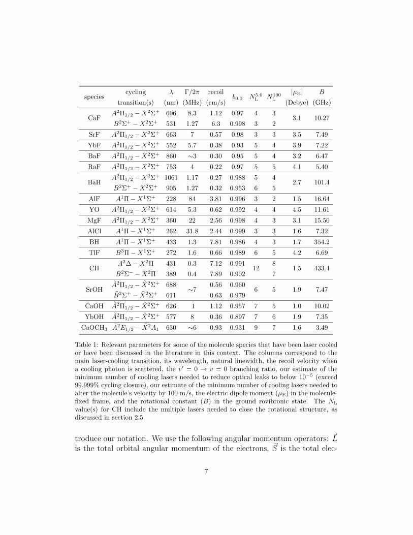
Table 1 presents some relevant parameters for a selection of moleculesamenable to laser cooling. In addition to some basic molecular constants,we have included a parameter N5.0

L , our estimate of the minimum numberof lasers needed to keep a molecule in the cooling cycle in 99.999% of allphoton scattering events. Similarly, we have included N100

L , our estimate ofthe minimum number of lasers needed to scatter enough photons to alter themolecule’s velocity by 100 m/s. We stress that this list is not exhaustiveand that new candidate molecules are being identified and characterized at asignificant pace, both in terms of their suitability for laser cooling and theirpotential applications.

2.2. Notation for molecular structure

Molecular structure is discussed in detail in several text books, e.g. Brownand Carrington (2003). Here, we briefly outline some salient points and in-

6

speciescycling λ Γ/2π recoil

b0,0 N5.0L N100

L

|µE| B

transition(s) (nm) (MHz) (cm/s) (Debye) (GHz)

CaFA2Π1/2 −X2Σ+ 606 8.3 1.12 0.97 4 3

3.1 10.27B2Σ+ −X2Σ+ 531 1.27 6.3 0.998 3 2

SrF A2Π1/2 −X2Σ+ 663 7 0.57 0.98 3 3 3.5 7.49

YbF A2Π1/2 −X2Σ+ 552 5.7 0.38 0.93 5 4 3.9 7.22

BaF A2Π1/2 −X2Σ+ 860 ∼3 0.30 0.95 5 4 3.2 6.47

RaF A2Π1/2 −X2Σ+ 753 4 0.22 0.97 5 5 4.1 5.40

BaHA2Π1/2 −X2Σ+ 1061 1.17 0.27 0.988 5 4

2.7 101.4B2Σ+ −X2Σ+ 905 1.27 0.32 0.953 6 5

AlF A1Π−X1Σ+ 228 84 3.81 0.996 3 2 1.5 16.64

YO A2Π1/2 −X2Σ+ 614 5.3 0.62 0.992 4 4 4.5 11.61

MgF A2Π1/2 −X2Σ+ 360 22 2.56 0.998 4 3 3.1 15.50

AlCl A1Π−X1Σ+ 262 31.8 2.44 0.999 3 3 1.6 7.32

BH A1Π−X1Σ+ 433 1.3 7.81 0.986 4 3 1.7 354.2

TlF B3Π−X1Σ+ 272 1.6 0.66 0.989 6 5 4.2 6.69

CHA2∆−X2Π 431 0.3 7.12 0.991

128

1.5 433.4B2Σ− −X2Π 389 0.4 7.89 0.902 7

SrOHA2Π1/2 − X2Σ+ 688

∼70.56 0.960

6 5 1.9 7.47B2Σ+ − X2Σ+ 611 0.63 0.979

CaOH A2Π1/2 − X2Σ+ 626 1 1.12 0.957 7 5 1.0 10.02

YbOH A2Π1/2 − X2Σ+ 577 8 0.36 0.897 7 6 1.9 7.35

CaOCH3 A2E1/2 − X2A1 630 ∼6 0.93 0.931 9 7 1.6 3.49

Table 1: Relevant parameters for some of the molecule species that have been laser cooledor have been discussed in the literature in this context. The columns correspond to themain laser-cooling transition, its wavelength, natural linewidth, the recoil velocity whena cooling photon is scattered, the v′ = 0 → v = 0 branching ratio, our estimate of theminimum number of cooling lasers needed to reduce optical leaks to below 10−5 (exceed99.999% cycling closure), our estimate of the minimum number of cooling lasers needed toalter the molecule’s velocity by 100 m/s, the electric dipole moment (µE) in the molecule-fixed frame, and the rotational constant (B) in the ground rovibronic state. The NL

value(s) for CH include the multiple lasers needed to close the rotational structure, asdiscussed in section 2.5.

troduce our notation. We use the following angular momentum operators: ~Lis the total orbital angular momentum of the electrons, ~S is the total elec-

7

tron spin, ~I =∑

i~Ii is the total nuclear spin and ~Ii is the spin of nucleus i,

~R is the rotational angular momentum of the molecule, ~N = ~L + ~R is thetotal angular momentum neglecting spin, ~J = ~N + ~S is the total angularmomentum apart from nuclear spin, and ~F = ~J + ~I is the total angularmomentum. The quantum numbers for the projections of ~L, ~S and ~J ontothe internuclear axis are Λ, Σ and Ω, respectively. The quantum number forthe projection of angular momentum X onto the space-fixed z-axis is mX .We use p to denote the parity. Primes are attached to quantum numbers ofexcited states. Molecular term symbols,1 used to denote a particular elec-tronic state, are expressed as 2S+1Λ

+/−Ω where Λ = 0, 1, 2, . . . are denoted as

Σ,Π,∆, . . . respectively and the +/− superscript, used only for Σ states,gives the reflection symmetry through a plane containing the internuclearaxis.2 Electronic states are conventionally given an additional single-letterlabel where X denotes the ground state, e.g. X2Σ+. Excited states of thesame (different) spin multiplicity as the ground state are labelled A,B, . . .(a, b, . . .), nominally in order of ascending energy. For polyatomic molecules,the letter label is usually decorated as A, B, . . . to avoid confusion with sym-metry groups of the same notation. We note that these conventions are onlyloosely followed and that the alphabetical labelling sequence often goes awry,especially for heavy molecules.

Recall that in the Born-Oppenheimer approximation the energy eigen-functions of a diatomic molecule are written as a product of an electronicpart φn(~RN ; ~ri), a vibrational part 1

RNfv(RN), and a rotational part de-

scribed by the spherical harmonic functions YR,mR(Θ,Φ):

ψn,v,R,mR(~RN ; ~ri) =1

RN

φn(~RN ; ~ri) fv(RN)YR,mR(Θ,Φ). (1)

Here, n is the set of quantum numbers labelling the electronic state, v labelsthe vibrational state, the vector ~RN describes the relative displacement ofthe nuclei and has spherical polar components (RN ,Θ,Φ), and we use ~rito refer to the set of all electronic coordinates. The φn satisfy the electronicSchrodinger equation obtained by fixing the nuclei in place, so is a functionof the ~ri and depends on ~RN as a parameter.

1In this work, we consider only heteronuclear molecules. Homonuclear molecules havean extra reflection symmetry, which is denoted as an additional g/u subscript.

2Electronic states with Λ = 0 (Σ states) should not be confused with the projection of~S onto the internuclear axis, also denoted Σ. The distinction should be clear by context.

8

In a molecule, the various angular momenta are often coupled together,and the most appropriate choice of basis states depends on the relative cou-pling strengths. In the limits where certain couplings dominate the interac-tion, we obtain the well-known Hund’s coupling cases (Herzberg, 1989). Fora state with Λ 6= 0 and S 6= 0, the Hamiltonian describing the spin-orbitinteraction and the rotational energy is Hrso = A~L · ~S+B ~R2. When A B,the state splits into spin-orbit manifolds of well-defined Ω, each of which hasa set of rotational levels labelled by J . This is Hund’s case (a), and we writethe eigenstates using the notation |n, v, J,Ω,mJ〉. When A B, the statesplits into rotational levels labelled by N , each of which is then split intospin-orbit levels labelled by J . This is Hund’s case (b) and we write theeigenstates using the notation |n, v,N, J,mJ〉. For Σ states with S 6= 0 thereis no spin-orbit interaction but there is an equivalent spin-rotation interac-tion, γ ~N · ~S, which again splits rotational states into levels labelled by J .When Λ 6= 0, the states of definite parity are linear combinations of +Λ and−Λ. Due to their interaction with Σ states, these parity eigenstates are notquite degenerate. This is Λ-doubling.

2.3. Transition strengths and selection rules

The intensity of an electric dipole transition between initial and finalstates is proportional to ω3

if |~dif |2, where ωif is the transition frequency and

~dif = 〈n′, v′, J ′,Ω′,m′J |~d|n, v, J,Ω,mJ〉. (2)

Here, ~d is the dipole moment operator, which we can write as ~d =∑

p dpe∗p

where e are the spherical basis vectors.To evaluate this matrix element, it is helpful to rotate the coordinate

system so that the axes align with those of the molecule (for a diatomicmolecule, the new z axis will lie along the internuclear axis). We introduce

the dipole moment operator in this rotated frame, ~µ, which is related to ~dby

dp =1∑

q=−1

D(1)∗p,q (Θ,Φ)µq. (3)

Here, p and q refer to spherical tensor components and D(1) is the rotationoperator. This gives us

~dif =∑p

e∗p∑q

Mp,q〈n′, v′|µq|n, v〉 (4)

9

whereMp,q = 〈J ′,Ω′,m′J |D(1)∗

p,q |J,Ω,mJ〉 (5)

depends only on angular coordinates and dictates the angular momentumselection rules, and

〈n′, v′|µq|n, v〉 =

∫ (1

RN

φ∗n′f ∗v′

)µq

(1

RN

φnfv

)R2N dRNd~r1 d~r2...d~rn. (6)

The integral form in equation (6) makes the coordinate dependence clearand highlights that 〈n′, v′|µq|n, v〉 does not depend on Θ and Φ. Next, weintroduce the quantity

µn′,nq (RN) = 〈n′|µq|n〉 =

∫φ∗n′(~RN ; ~ri)µq φn(~RN ; ~ri) d~r1 d~r2...d~rn. (7)

When n′ = n, this is the dipole moment for state n, which we write as µnq (RN)without the second superscript. Its value at the equilibrium separation, R0,is usually called the permanent dipole moment of the molecule in state n.When n′ 6= n, equation (7) is the transition dipole moment function for thetransition between n and n′. The transition dipole moment can be calculatedusing a variety of quantum chemistry techniques, e.g. Hickey and Rowley(2014), or can be determined experimentally by measuring the transitionrate.

Equation (4) can now be written as

~dif =∑p

e∗p∑q

Mp,q

∫f ∗v′(RN)µn

′,nq (RN)fv(RN)dRN . (8)

We can expand µn′,nq around the equilibrium separation R0 giving

µn′,nq (RN) ' µn

′,nq (R0) +

dµn′,nq

dRN

∣∣∣∣∣R0

(RN −R0) + . . . . (9)

The first term usually dominates in this expansion, in which case we have

~dif '∑p

e∗p∑q

Mp,q × µn′,nq (R0)×

∫f ∗v′fvdRN . (10)

10

X 2Σ+

A 2Π1/2

3.0 3.5 4.0 4.5 5.0

0

5000

10000

15000

20000

25000

30000

35000

Nuclear separation (a0)

Energy(cm

-1)

Figure 1: RKR potentials for the X2Σ+ and A2Π1/2 states of CaF, calculated using themolecular constants given in Kaledin et al. (1999). The low-lying vibrational states arealso shown.

The last factor in equation (10) is the overlap integral between vibrationalstate v′ in electronic state n′ and vibrational state v in electronic state n.The square of this overlap integral,

qv′,v =

∣∣∣∣∫ f ∗v′fvdRN

∣∣∣∣2 , (11)

is the Franck-Condon factor.

2.4. Vibrational branching ratios

To a good approximation, the vibrational branching ratio for the transi-tion from v′ to v when the molecule decays from n′ to n is

bv′,v =qv′,vω

3v′,v∑

v′′ qv′,v′′ω3v′,v′′

(12)

where ωv′,v′′ is the transition frequency. However, it is worth noting thatthe terms in equation (9) beyond the first can sometimes alter the branching

11

ratios significantly. Laser cooling is easier when the number of vibrationalbranches that need to be addressed is small. For most experiments, theleak out of the cooling cycle must be reduced below 10−5 or 10−6. The bestsystems have bv′,v=v′ ≈ 1, with branching ratios that diminish very rapidly as|v−v′| increases. This occurs when the potentials for the two electronic statesare nearly the same. Examples include the alkaline earth monofluorides andmonohydroxides, where the valence electron is localized on the metal atomand has little influence on the bonding.

The branching ratios between low-lying vibrational states, where anhar-monic effects are small, can be estimated using a harmonic oscillator ap-proximation. Here, harmonic oscillator eigenfunctions are used to evaluatethe overlap integral in equation (11). For each electronic state, the eigen-functions are characterised by just two parameters, the harmonic frequencyωe, and the equilibrium separation R0. The first is identical to the vibra-tional constant, and the second can be found from the rotational constantBe = ~2/(2mrR

20) where mr is the reduced mass. When Be is similar for the

two electronic states, and so too is ωe, the branching ratios will be favourable.Table 2 shows the branching ratios calculated for the A2Π1/2(v′)→ X2Σ+(v)transitions of CaF. The first (top) entry in each case is the value calculatedusing the harmonic oscillator approximation. The values on the diagonals areclose to 1, and the branching ratios diminish rapidly away from the diagonals,showing that this is a favourable system for laser cooling.

A more accurate set of branching ratios can be determined using Rydberg-Klein-Rees (RKR) potentials. The RKR potential is constructed from mea-sured band spectra, which are typically parameterized using a small numberof molecular constants. The procedure, as described for example by Rees(1947) and Le Roy (2016), is straightforward to implement. As an exam-ple, figure 1 shows the RKR potentials for the X2Σ+ and A2Π1/2 states ofCaF, calculated using the molecular constants given in Kaledin et al. (1999).The eigenfunctions of the Hamiltonian can then be calculated numericallyfor these potentials, followed by the overlap integral of equation (11). Thesecond entries in the set of branching ratios given in table 2 are the valuescalculated using this procedure. Comparing to the harmonic oscillator re-sults, we see that the fractional change is small for the larger values of bv′,v,but sometimes very large for the small values. For example, b0,3 increases bytwo orders of magnitude and becomes non-negligible for laser cooling. Thishighlights the importance of using accurate potentials to estimate branchingratios, or measuring the branching ratios directly, in designing any laser cool-

12

v = 0 v = 1 v = 2 v = 3 v = 4

9.80× 10−1 1.96× 10−2 1.18× 10−4 1.42× 10−7 2.27× 10−10

v′ = 0 9.80× 10−1 1.95× 10−2 6.00× 10−4 2.22× 10−5 9.60× 10−7

9.77× 10−1 2.21× 10−2 7.15× 10−4 2.75× 10−5 1.22× 10−6

2.39× 10−2 9.37× 10−1 3.86× 10−2 3.53× 10−4 5.75× 10−7

v′ = 1 2.49× 10−2 9.37× 10−1 3.68× 10−2 1.70× 10−3 8.42× 10−5

2.17× 10−2 9.34× 10−1 4.19× 10−2 2.04× 10−3 1.05× 10−4

4.37× 10−4 4.65× 10−2 8.95× 10−1 5.69× 10−2 7.03× 10−4

v′ = 2 1.59× 10−5 4.86× 10−2 8.96× 10−1 5.21× 10−2 3.22× 10−3

4.95× 10−6 4.24× 10−2 8.94× 10−1 5.95× 10−2 3.87× 10−3

6.60× 10−6 1.28× 10−3 6.78× 10−2 8.55× 10−1 7.47× 10−2

v′ = 3 4.29× 10−7 4.19× 10−5 7.11× 10−2 8.58× 10−1 6.56× 10−2

3.89× 10−7 1.19× 10−5 6.20× 10−2 8.56× 10−1 7.52× 10−2

8.88× 10−8 2.59× 10−5 2.51× 10−3 8.79× 10−2 8.16× 10−1

v′ = 4 1.16× 10−9 1.72× 10−6 7.28× 10−5 9.26× 10−2 8.23× 10−1

1.87× 10−9 1.55× 10−6 1.84× 10−5 8.08× 10−2 8.21× 10−1

Table 2: Vibrational branching ratios, bv′,v for the A2Π1/2(v′)→ X2Σ+(v) transitions ofCaF. There are three entries for each value. The first is calculated using the harmonicoscillator approximation, the second using the RKR potential and only the first term inequation (9), and the third using the RKR potential and the transition dipole momentfunction, µn

′,n(RN ) given in Pelegrini et al. (2005).

ing scheme. If the RN -dependence of the transition dipole moment is known,even higher accuracy can be obtained for the branching ratios by evaluatingthe integral appearing in equation (8) instead of its approximate form. Thethird entries in table 2 are obtained using this approach. In this example,the inclusion of the RN -dependence of µn

′,n makes relatively minor changesto most of the branching ratios.

2.5. Closed rotational transitions

The angular factor in equation (8) is

Mp,q = 〈J ′,Ω′,m′J |D(1)∗p,q |J,Ω,mJ〉

= (−1)2J ′−m′J−Ω′√

(2J + 1)(2J ′ + 1)

×(

J ′ 1 J−m′J p mJ

)(J ′ 1 J−Ω′ q Ω

). (13)

13

This equation gives the relative intensities of rotational branches betweencase (a) basis states. A similar expression can be written down for case (b)basis states (Brown and Carrington, 2003). We see from equation (13) thatthe selection rule on J is ∆J = J − J ′ = 0,±1, except in the case whereΩ′ = Ω = 0 where it is restricted to ∆J = ±1. In addition, we have theusual selection rule that parity must change in an electric dipole transition.

The selection rule on J implies that an excited state can decay on up tothree rotational branches. However, a careful choice of transition can limitthis to just a single rotational branch (Stuhl et al., 2008). Figure 2 showshow to avoid rotational branching for several electronic transitions. Thesimplest is a 1Σ− 1Σ transition, as shown in (a). Each rotational level of theupper state can decay to two levels in the lower state, following the ∆J = ±1selection rule. The exception is J ′ = 0, which can only decay to J = 1, so thetransition 1Σ(J ′ = 0)− 1Σ(J = 1) is rotationally closed. Figure 2(b) shows a2Σ− 2Σ transition. Here, the spin-rotation interaction splits each rotationallevel (apart from N = 0) into a pair of levels with J = N ± 1/2. The lasercooling transition is the same as in (a), but the excited state (J ′ = 1/2)can decay to both the J = 1/2 and J = 3/2 components of N = 1. Bothcomponents have to be addressed by the laser light, but the spin-rotationsplitting is usually small enough that this can easily be done by adding anrf sideband to the laser. An example, already used for laser cooling (Truppeet al., 2017a), is the B2Σ+ −X2Σ+ transition of CaF.

The situation is different for a 1Π−1Σ transition, illustrated in figure 2(c).Here, Λ-doubling in the upper state leads to a pair of states of oppositeparity for each value of J ′. For every J ′, one parity component can decay totwo lower levels, while the other can only decay to a single lower level. Itfollows that the 1Π(J ′ = J) − 1Σ(J) transitions (i.e. Q-branch transitions)are rotationally closed for all J . Thus, all lower levels other than J = 0could be used for laser cooling. AlCl and AlF are good examples of laser-coolable molecules with this structure, and experiments to cool these speciesare currently being built (Truppe et al., 2019; Hemmerling, 2020). Note thatheavy molecules such as TlF can be cooled using a 3Π1−1Σ transition (Hunteret al., 2012), which has the same structure as the 1Π − 1Σ case. For lightermolecules such as AlF, the 3Π1– 1Σ transition could be used for narrow-linecooling to temperatures near the recoil limit (Truppe et al., 2019).

Figure 2(d) shows a 2Π –2Σ transition. Here, we have assumed thatthe spin-orbit splitting of the excited state is much larger than the rotationalsplitting (A B), and we focus on the 2Π1/2 manifold that is of most interest

14

1/2

1/21/23/2

3/2

0

1

2 3/25/2

1

0

012

1

012

23/2

1/2

1/21/23/2

1

01/2

0

1

2 3/25/2

3/2

1/2

1

01/2

1

2

3

1/2

3/23/2

5/2

5/27/2

Figure 2: Rotationally-closed components of various transitions, including excitations(solid vertical arrows) and decays (dashed vertical arrows). Energy levels are colour codedaccording to their parity p, being light blue for negative parity (p = −1) and dark purplefor positive parity (p = 1). (a) 1Σ − 1Σ. (b) 2Σ − 2Σ. Both components shown have tobe addressed. (c) 1Π− 1Σ. Either of the transitions indicated, or any of the others in thesame sequence, can be used. (d) 2Π− 2Σ. Both components shown have to be addressed.(e) 2Σ − 2Π. All three components shown have to be addressed, unless A B in whichcase the rightmost transition is forbidden.

for laser cooling. Λ-doubling splits the rotational levels of 2Π1/2 into states ofopposite parity, and the spin-rotation interaction splits the rotational levelsof 2Σ into pairs of the same parity. The transition 2Π1/2(J ′ = 1/2, p =

15

−1) − 2Σ+(N = 1) is rotationally closed. As before, both spin-rotationcomponents of the transition have to be addressed. All the molecules lasercooled so far have this structure.

As a final example, figure 2(e) shows a 2Σ − 2Π transition. For conve-nience, we have used a case (b) notation where rotational levels, distinguishedby N , are split by the spin-orbit interaction into pairs labelled by J , and theseare split further into opposite parity Λ-doublets. In this case, the transition2Σ(N ′ = 0) − 2Π(N = 1) is rotationally closed, provided both spin-orbitcomponents are addressed. However, 2Π states are often closer to case (a)states, or have similar values of A and B so do not conform to either couplingcase. In this case, the transition to the state labelled as (N = 2, J = 3/2)is allowed and must also be addressed for laser cooling to work. This case isawkward because the splittings are typically too large to be addressable withmodulators, calling for three separate lasers for each vibrational branch. TheB2Σ− −X2Π transition of CH is an interesting example. The ground statehas A/B = 1.984 and the branching ratios for the three transitions shown infigure 2(e) are in the ratio (from left to right) 0.333:0.623:0.044. The weakbranch falls below 10−3 for A/B < 0.35 and below 10−4 for A/B < 0.11.

2.6. Hyperfine structure

An understanding of the hyperfine structure is important for designing alaser cooling scheme. The hyperfine states can also be a useful resource forcontrolling collisions and for quantum simulation and information processing.

2.6.1. Hyperfine interactions

The relevant terms in the hyperfine Hamiltonian depend on the elec-tronic state and on the nuclear spins. A thorough treatment of these termstogether with expressions for their matrix elements can be found in Brownand Carrington (2003). The main terms, and the ones most relevant to ourdiscussion, are

16

HSN = γ~S · ~N, (14a)

HIL =∑i

ai~Ii · ~L, (14b)

HIS =∑i

biF~Ii · ~S + ti√

6T 2(C) · T 2(~Ii, ~S), (14c)

HIN =∑i

ciI~Ii · ~N, (14d)

HQ =∑i

−eT 2(∇ ~E) · T 2(Qi), (14e)

HII = c4~I1 · ~I2 − c3

√6T 2(C) · T 2(~I1, ~I2). (14f)

The summation is over the nuclei. HSN is the electron spin-rotation inter-action. It is not strictly a hyperfine interaction since it does not involve thenuclear spins, but it is often of a similar magnitude to other terms in thehyperfine Hamiltonian so must be treated together with them. HIL is theorbital hyperfine interaction describing the interaction of the nuclear mag-netic moments with the magnetic field at the nuclei produced by the orbitalmotion of the electrons. It is relevant for electronic states with Λ > 0. Theinteraction between the electron and nuclear magnetic moments, HIS hastwo parts, the Fermi contact part and the electron-nuclear spin dipolar in-teraction. These terms are sometimes expressed using the parameters b andc introduced by Frosch and Foley (1952), the relation being bF = b + c/3and t = c/3. The dipolar interaction in equation (14c) is written as the

scalar product of two rank-2 spherical tensors; T 2(~I, ~S) is the one formed

from ~I and ~S, while T 2(C) is a spherical tensor whose components are therenormalised spherical harmonics C2

q =√

4π/5Y2,q(Θ,Φ). HIN is the nu-clear spin-rotation interaction. HQ is the interaction between the electricquadrupole moments of the nuclei and the electric field gradient at the nu-clei. For each nucleus, two parameters appear in the matrix elements of HQ,eq0Q and eq2Q. Here, eQ is the nuclear quadrupole moment, q0 is the electricfield gradient in the direction of the internuclear axis, and q2 is the gradientin the perpendicular direction and is only relevant for states with Λ > 0. Fi-nally, HII represents the tensor and scalar interactions between the nucleardipole moments associated with the two nuclear spins I1 and I2.

17

2.6.2. Examples of hyperfine structure

Now let us consider some relevant examples. We first look at a 2Σ di-atomic molecule having one nucleus of zero spin and the other with spinI = 1/2. This is the structure of ground-state alkaline-earth monohydridesand monofluorides. The hyperfine Hamiltonian is

Hhyp = HSN +HIS +HIN . (15)

Figure 3(a) shows the example of CaF in the state X2Σ+(v = 0, N = 1),which is the lower level of the main laser cooling transition. To calculatethe energies, we have used equation (15) and the parameters from Childset al. (1981). The spin-rotation interaction splits N = 1 into two levels withJ = 1/2 and J = 3/2, and these are further split by the interaction withthe nuclear spin, resulting in the four hyperfine levels shown. Since HSN andHIS have similar magnitudes, the two F = 1 states are mixtures of J = 1/2and 3/2.

Our second example is a 1Σ diatomic molecule. Here, because thereis no electron spin, the hyperfine structure is much smaller and is typicallydominated by the electric quadrupole interaction. The hyperfine Hamiltonianis

Hhyp = HQ +HIN +HII . (16)

Figure 3(b) shows the example of AlF in the state X1Σ+(v = 0, N = 1), thelower level of the laser cooling transition. To calculate the energies, we haveused equation (16) and the parameters from Truppe et al. (2019). The mainsplitting is due to the electric quadrupole moment of the Al nucleus, whichhas I1 = 5/2. This splits N = 1 into three levels with F1 = 3/2, 5/2, 7/2,

where we have introduced the intermediate angular momentum ~F1 = ~N + ~I1.The contribution to this splitting from the term ~I1. ~N is very much smaller.The F nucleus has no quadrupole moment, since it has I2 = 1/2. Each

F1 level is split in two by the term ~I2. ~N , resulting in the structure shown.Because these latter splittings are much smaller, all the states can be labelledby F1 and F . The contribution of HII is even smaller and is most relevantfor the ground rotational state, N = 0, where both HQ and HIN are absent.

For laser cooling, all hyperfine components of the rotationally closed tran-sition need to be addressed for each vibrational branch. Because the hyper-fine splittings are fairly small, this can usually be done by using acousto-opticand/or electro-optic modulators to add the relevant sidebands to the lasers.

18

N=1

F=1

F=0

F=1

F=2

0

76.257

122.920

147.824

N=1

F1=5/2

F1=7/2

F1=3/2

F=3

F=2

F=3

F=4

F=2

F=1

00.004

7.892

7.940

11.22611.247

(a) CaF (b) AlF

Figure 3: Hyperfine structure in the N = 1 levels of (a) CaF X2Σ+(v = 0) and (b) AlFX1Σ+(v = 0). The energies are given in MHz relative to the lowest hyperfine level.

In cases where the splitting exceeds 1 GHz this becomes more difficult andit may be necessary to use separate lasers.

2.6.3. Hyperfine-induced transitions

The electron-nuclear spin dipolar interaction in HIS has matrix elementscoupling states of the same F in rotational states N and N ± 2. This canresult in a small leak out of the cooling cycle. To estimate the size of this leak,consider again the case of a 2Σ molecule with a single nuclear spin I = 1/2.The state |N, J, F 〉 = |3, 5/2, 2〉 acquires a small admixture of |1, 3/2, 2〉 dueto the hyperfine interaction,

|3, 5/2, 2〉 = |3, 5/2, 2〉0 + ε|1, 3/2, 2〉0, (17)

where the subscript 0 indicates the unperturbed state and

ε =0〈1, 3/2, 2|HIS|3, 5/2, 2〉0

E3 − E1

=3

50

√3

2

t

B. (18)

Here, EN is the unperturbed energy of rotational manifold N . The prob-

ability of decaying to |3, 5/2, 2〉 is ε2 = 275000

(tB

)2times the probability of

decaying to |1, 3/2, 2〉. For CaF, this is 9× 10−8, which is negligible in mostsituations. The electric quadrupole interaction (when it exists) also results

19

in a leak to N = 3 but this is typically even smaller. Hyperfine interactionsin the excited state have a similar influence and are likely to dominate in thecase of a 1Π − 1Σ transition since the hyperfine interaction is usually muchlarger in the 1Π state.

2.7. Dark states

As illustrated in figure 2, laser cooling of molecules always involves tran-sitions where F ′ ≤ F .3 In this situation there are dark states, which arestates of the molecule that do not couple to the light field. Stated anotherway, they are stationary states of the combined molecule-light system thathave no excited state component. A molecule will be optically pumped intoa dark state after scattering only a small number of photons. This is an im-pediment to laser cooling that has to be overcome by destabilizing the darkstates. Conversely, dark states can be a useful resource for cooling moleculesto very low temperature because they play a key role in sub-Doppler coolingmechanisms and because a molecule in a dark state is not heated by photonscattering. In this case, rather than destabilizing the dark states, it is usefulto engineer ones that are robust.

To identify the dark states, let us consider a molecule with a set of groundstates |γ, F,M〉 with energies ~ωF and a set of excited states |γ′, F ′,m′〉 withenergies ~ωF ′ . Here, γ and γ′ represent other quantum numbers neededto label the states. The Hamiltonian is H = H0 +

∑iHi where H0 =∑

F,m ~ωF |γ, F,m〉〈γ, F,m|+∑

F ′,m′ ~ωF ′ |γ′, F ′,m′〉〈γ′, F ′,m′| and Hi = −~d·~E i. Here, ~E i is the field due to a laser of frequency ωi and wavevector ~ki. Weexpand the wavefunction in terms of the field-free eigenstates,

|ψ(t)〉 =∑F,m

aF,m(t)e−iωF t|γ, F,m〉+∑F ′,m′

aF ′,m′(t)e−iωF ′ t|γ′, F ′,m′〉. (19)

The Schrodinger equation is

i~∑F,m

daF,mdt

e−iωF t|γ, F,m〉+ i~∑F ′,m′

daF ′,m′

dte−iωF ′ t|γ′, F ′,m′〉

=∑i,F,m

HiaF,me−iωF t|γ, F,m〉+

∑i,F ′,m′

HiaF ′,m′e−iωF ′ t|γ′, F ′,m′〉. (20)

3Transitions where F ′ > F are called type-I and those where F ′ ≤ F are type-II.

20

A dark state must have aF ′,m′ = 0 for all F ′ and m′. Applying this condition,and multiplying from the left by 〈γ′, F ′,m′|eiωF ′ t, we obtain∑

i,F,m

aF,mei(ωF ′−ωF )t〈γ′, F ′,m′|Hi|γ, F,m〉 = 0. (21)

Writing ~E i = ~Ei cos(ωit), then making the rotating wave approximation andintroducing ∆i,F,F ′ = ωi − (ωF ′ − ωF ), this becomes∑

i,F,m

aF,me−i∆i,F,F ′ t〈γ′, F ′,m′|~d · ~Ei|γ, F,m〉 = 0. (22)

Expanding the scalar product and using the Wigner-Eckart theorem, wereach the condition∑i,F,m,q

aF,me−i∆i,F,F ′ t(−1)q+F

′−m′(

F ′ 1 F−m′ q m

)〈γ′, F ′||d||γ, F 〉Ei

−q = 0,

(23)

for all F ′,m′. This condition can be expressed in the form ~A ·~a = 0, where ~ais the vector of the coefficients aF,m and ~A is the matrix whose elements are

A(F ′,m′),(F,m) =∑i,q

e−i∆i,F,F ′ t(−1)q+F′−m′

(F ′ 1 F−m′ q m

)〈γ′, F ′||d||γ, F 〉Ei

−q.

(24)

This is equivalent to finding the set of vectors that span the null space of ~A.This procedure can be used to find the dark states for any set of ground andexcited states and any light field. Note, however, that it does not guaranteethat the dark states are time-independent; this has to be checked separately.

Let us consider the simple case of a molecule with just a single groundlevel, F , and a single excited level, F ′, driven by a single frequency oflight. Table 3 presents the results for certain special choices of polariza-tion. Columns 3 and 4 correspond to light that drives σ− and π transitionsrespectively, and here the dark states are the obvious ones. In column 5, thelight is linearly polarized along x when θ = π/2, linearly polarized along ywhen θ = 0, and corresponds to the standard one-dimensional σ+σ− config-uration when θ = kz. This is an important case since it is frequently usedto model sub-Doppler cooling processes. The final column, with θ = kz,corresponds to a pair of beams counter-propagating along z and linearly po-larized at an arbitrary angle φ to one another. This is another important

21

(E−1, E0, E+1)

F F ′ (0, 0, 1) (0, 1, 0) −i√2(eiθ, 0, e−iθ) 1√

2(−c+, 0, c−)

12

12 (1, 0) None None None

1 0(0, 1, 0) (0, 0, 1) (0, 1, 0) (0, 1, 0)

(1, 0, 0) (1, 0, 0) (−e−iθ, 0, eiθ) (c−, 0, c+)

1 1 (1, 0, 0) (0, 1, 0) (e−iθ, 0, eiθ) (−c−, 0, c+)

32

12

(1, 0, 0, 0) (1, 0, 0, 0) (−e−iθ, 0,√

3eiθ, 0) (c−, 0,√

3c+, 0)

(0, 1, 0, 0) (0, 0, 0, 1) (0,−√

3e−iθ, 0, eiθ) (0,√

3c−, 0, c+)

32

32 (1, 0, 0, 0) None None None

2 1(1, 0, 0, 0, 0) (1, 0, 0, 0, 0) (0,−e−iθ, 0, eiθ, 0) (0, c−, 0, c+, 0)

(0, 1, 0, 0, 0) (0, 0, 0, 0, 1) (e−2iθ, 0,−√

6, 0, e2iθ) (c2−, 0,√

6c−c+, 0, c2+)

2 2 (1, 0, 0, 0, 0) (0, 0, 1, 0, 0) (√

3e−2iθ, 0,√

2, 0,√

3e2iθ) (√

3c2−, 0,−√

2c−c+, 0,√

3c2+)

Table 3: Dark states for single ground and excited levels, with respective angular momentaF and F ′, for various polarization choices expressed as (E−1, E0, E+1). The dark statesare expressed in the form (aF,m=−F , ...aF,m=F ) and are not normalised. We have used the

notation c± = cos[θ ± φ2 ].

case in the context of sub-Doppler cooling, and is discussed in section 3.2.2.We note that in the last two cases the dark states are position dependent. Adark molecule moving sufficiently slowly through the light field will adiabat-ically follow the changing polarization and remain dark, but if the moleculeis moving too quickly, it will not stay in the dark state. We can also ex-tend this discussion to a pair of laser beams with different frequencies. Ifthe two frequency components have the same polarization there will still bestationary dark states (the same number as for a single frequency). Thereare typically no stationary dark states when the polarizations of the two fre-quency components are different. There are exceptions to this rule however.For example, if both components have E−1 = 0, or both have E+1 = 0, therewill be a dark state when F ′ = F − 1.

2.7.1. Destabilizing dark states

To maintain a high rate of photon scattering, it is necessary to destabilizethe dark states, preferably at a rate that is comparable to the Rabi frequency.There are several ways to do this. One way, already discussed above, is toensure that the polarization of the light field varies with position. In this

22

case the dark states will also be position dependent, and molecules will notremain in the dark state if they are moving quickly enough. The requirementon the speed is discussed in the context of sub-Doppler cooling in section3.2.2. In other cases, a more active method of destabilization is needed.For example, radiation pressure slowing of a molecular beam (see section 4)usually involves a single counter-propagating laser beam resulting in uniformpolarization, and active destabilization of dark states is crucial.

As discussed in detail in Berkeland and Boshier (2002), dark states canbe made time-dependent either by modulating the polarization of the light,or by applying a magnetic field. Destabilization by polarization modulationis intuitively clear, since the dark state depends on the polarization. Foran intuitive picture of destabilization by a magnetic field, take the z-axisalong the magnetic field and choose the polarization of the light so thatthe dark states are superpositions of different m sub-levels. The energiesof neighbouring sub-levels differ by the Zeeman splitting, ~ωZ, so the darkstate evolves in time. The system has three characteristic rates - the decayrate of the excited state, Γ, the Rabi frequency, Ω, and the rate at whichthe dark state evolves into a bright state, γd→b. The approximate value ofγd→b is either ωZ or the polarization modulation rate. The photon scatteringrate is small when γd→b Ω since the molecule adiabatically follows theslowly-varying dark state. It is also small when γd→b Ω because then thelight is detuned from resonance. For any Ω, the maximum scattering rateis reached when γd→b ≈ Ω/2, and the global maximum is approached whensatisfying that condition together with Ω Γ.

There are also some cases where dark states are not destabilized by ei-ther a magnetic field or polarization modulation. As an example, considera linear superposition of three states, all with m = 1, coming from threedifferent hyperfine components of the ground state, and coupled to an ex-cited state with F ′ = 1. The state is obviously dark to σ+ polarization.There are only two remaining orthogonal polarizations, and the state hastwo free coefficients, so there must be a particular linear combination thatis dark to all three orthogonal polarizations. Polarization modulation willhave no influence on this dark state. If, in addition, the ground state has nomagnetic moment, a magnetic field will similarly have no influence. Being alinear combination of different hyperfine states, this dark state will evolve atthe hyperfine frequency, making it irrelevant if the hyperfine components areresolved. However, if the hyperfine splitting is very small compared to thenatural linewidth of the transition, this evolution will be slow, limiting the

23

1 2

F=1

F=2

F'=1F'=0

Δ

Δhfs

Figure 4: Engineering Raman dark states in a level scheme that is typical of many laser-coolable molecules.

scattering rate. This situation is exactly the one encountered for TlF drivenon the B3Π1 −X1Σ+ transition (Clayburn et al., 2018). The magnetic mo-ment of the 1Σ ground state is too small to be useful. The ground statehas the same hyperfine structure as shown in figure 3(a), except that theintervals are all very small, spanning only 220 kHz in total. Conversely, theexcited state has very large hyperfine structure, so a single laser frequencywill only couple to one hyperfine component of the excited state. These fea-tures conspire to produce a low scattering rate. This issue can be addressedby coupling to auxiliary states, for example using microwaves to couple toanother rotational level.

2.7.2. Engineering dark states

It is sometimes desirable to engineer dark states, especially to enhancesub-Doppler cooling and velocity-selective coherent population trapping (Cohen-Tannoudji, 1998; Cheuk et al., 2018; Caldwell et al., 2019). Dark states thatare superpositions of two lower levels (typically different hyperfine compo-nents) can be engineered using two laser components with relative frequenciessatisfying the Raman condition.

Figure 4 illustrates an example which is pertinent to many of the moleculeslaser cooled so far. Here, two ground hyperfine levels (F = 1, 2) are coupledby lasers to two excited hyperfine levels (F ′ = 0, 1). When the frequencydifference between the two lasers matches the ground state hyperfine inter-val, stationary dark states are formed, sometimes known as Raman darkstates. When both laser components are polarized to drive π transitions

24

there are two Raman dark states in this system, ±√

3/5 η|1,±1〉 + |2,±1〉.Here η = d2,1/d1,1 where dF,F ′ = 〈F ′||d||F 〉, and we have omitted the nor-malization. The equivalent superposition with m = 0 is not dark because|2, 0〉 only couples to F ′ = 1 while |1, 0〉 only couples to F ′ = 0. Whenboth laser components are polarized to drive σ− transitions there is a singleRaman dark state, −

√1/5 η|1, 0〉 + |2, 0〉. The superposition with m = 1 is

not dark because the |1, 1〉 state can couple to both F ′ = 1 and 0. Whenlaser component 1 drives σ+ transitions and component 2 drives σ− transi-tions the Raman dark state is

√6/5 η|1, 0〉 + |2, 2〉. It is important to note

that in constructing these dark states we have assumed that the ground statehyperfine interval is large compared to the laser detuning, ∆hfs ∆. Whenthis is not the case, off-resonant couplings (component 1(2) drives transitionsfrom F = 2(1)) result in residual coupling to the light and there will be somephoton scattering.

2.8. Intermediate electronic states

One of the desirable properties of a good cycling transition is the absenceof any intermediate electronic levels. This simplifies the cooling scheme.Nevertheless, molecules with intermediate states have been laser cooled, andit is interesting to look at these examples.

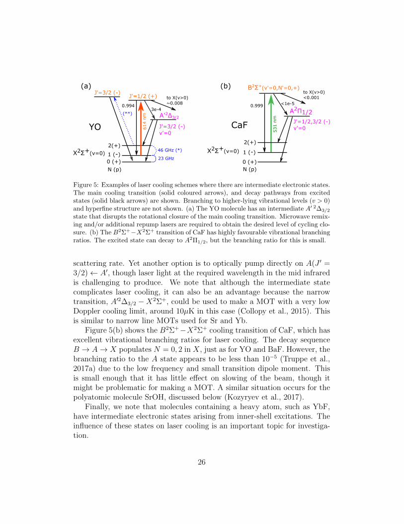
Molecules such as YO (Yeo et al., 2015) and BaF (Chen et al., 2016; Haoet al., 2019; Albrecht et al., 2020) have an intermediate ∆ state that canpotentially be troublesome. Figure 5(a) shows the laser cooling scheme usedto cool YO molecules (Collopy et al., 2018). The main cooling transition isA2Π1/2(v′ = 0, J ′ = 1/2)−X2Σ+(v = 0, N = 1) at 614 nm. Molecules excitedto the A state can decay to an intermediate A′ 2∆3/2 state after scatteringabout 3000 photons. Molecules that end up in A′ can decay to either N = 0or N = 2 of X2Σ+. Though electric dipole forbidden, this decay occurs witha lifetime of ≈1 µs due to mixing of the A′ state with the nearby A2Π3/2 state(not shown in the figure). Molecules that decay to N = 0 are re-introducedinto the cooling cycle using resonant microwaves at 23 GHz that mix the N =0 and N = 1 states. This increases the number of ground states participatingin the main cooling cycle and consequently reduces the overall scatteringrate, as explained in section 3.1. Molecules that decay to N = 2 can be re-introduced into the cooling cycle using resonant microwaves (indicated by (*)in the figure) at 46 GHz that mix N = 2 and N = 1, further decreasing thescattering rate by about a factor of two. Alternatively, they can be opticallyrepumped via A2Π1/2(J ′ = 3/2) (indicated by (**)) without affecting the

25

2(+)

1 (-)0 (+)

N (p)

23 GHz

46 GHz (*)X2Σ+(v=0)

A2Π1/2

J'=3/2 (-)J'=1/2 (+)

A'2Δ3/2

3e-40.994

614 n

m(**)

to X(v>0)~0.008

YO

(a)

J'=3/2 (-)v'=0

(b)

CaF

X2Σ+(v=0)

B2Σ+(v'=0,N'=0,+)

531 n

m

J'=1/2,3/2 (-)v'=0

0.999

to X(v>0)<0.001

<1e-5

2(+)

0 (+)

1 (-)

N (p)

Figure 5: Examples of laser cooling schemes where there are intermediate electronic states.The main cooling transition (solid coloured arrows), and decay pathways from excitedstates (solid black arrows) are shown. Branching to higher-lying vibrational levels (v > 0)and hyperfine structure are not shown. (a) The YO molecule has an intermediate A′ 2∆3/2

state that disrupts the rotational closure of the main cooling transition. Microwave remix-ing and/or additional repump lasers are required to obtain the desired level of cycling clo-sure. (b) The B2Σ+−X2Σ+ transition of CaF has highly favourable vibrational branchingratios. The excited state can decay to A2Π1/2, but the branching ratio for this is small.

scattering rate. Yet another option is to optically pump directly on A(J ′ =3/2)← A′, though laser light at the required wavelength in the mid infraredis challenging to produce. We note that although the intermediate statecomplicates laser cooling, it can also be an advantage because the narrowtransition, A′2∆3/2 −X2Σ+, could be used to make a MOT with a very lowDoppler cooling limit, around 10µK in this case (Collopy et al., 2015). Thisis similar to narrow line MOTs used for Sr and Yb.

Figure 5(b) shows the B2Σ+−X2Σ+ cooling transition of CaF, which hasexcellent vibrational branching ratios for laser cooling. The decay sequenceB → A→ X populates N = 0, 2 in X, just as for YO and BaF. However, thebranching ratio to the A state appears to be less than 10−5 (Truppe et al.,2017a) due to the low frequency and small transition dipole moment. Thisis small enough that it has little effect on slowing of the beam, though itmight be problematic for making a MOT. A similar situation occurs for thepolyatomic molecule SrOH, discussed below (Kozyryev et al., 2017).

Finally, we note that molecules containing a heavy atom, such as YbF,have intermediate electronic states arising from inner-shell excitations. Theinfluence of these states on laser cooling is an important topic for investiga-tion.

26

2.9. Polyatomic moleculesLaser cooling of polyatomic molecules is more complex than for diatomic

molecules due to the proliferation of vibrational modes. A molecule withn atoms has ξ = 3n − 6 vibrational modes, or ξ = 3n − 5 if the moleculeis linear. Furthermore, the dense level structure resulting from the manydegrees of freedom can lead to a breakdown of the Born-Oppenheimer ap-proximation, and thus to violations of rotational selection rules. Anharmonicterms in the vibrational Hamiltonian can also give rise to mixing betweendifferent vibrational modes. These complications present major challenges tolaser cooling of complex molecules. Nevertheless, there has been great recentprogress in this direction.

Initial ideas for identifying polyatomic species amenable to laser cool-ing were presented by Isaev and Berger (2016). In general, alkaline earthmonohydroxide (MOH) and monoalkoxide (MOR, where R is an organic sub-stituent) molecules with a heavy alkaline earth atom, e.g. M ∈ Sr,Ca,Yb,Ba,have been identified as particularly promising candidates. As in the diatomiccase, vibrational branching is suppressed when the potential energy surfacesof the ground and excited states are very similar. This is commonly satis-fied in alkaline earth monofluoride (MF) and monohydride (MH) diatomicspecies, where one valence electron of M forms the ionic bond and the othercan be excited without significantly affecting that bond. Certain atom com-plexes or ligands, e.g. OH, can replace F or H with much the same result– an optically active non-bonding electron having transitions with near di-agonal Franck-Condon factors. Specific ligands, e.g. OCH3, are expected tomake these factors even closer to unity than in the corresponding diatomicsystem (Dickerson et al., 2020).

Let us consider a linear triatomic monohydroxide molecule, MOH, thathas a X2Σ+ ground state. Being linear, this is in many ways very similarto the diatomic case, with electronic states associated with excitation of theM-centred electron and rotational states associated with end-over-end rota-tions. The most significant difference is the additional modes of vibration.In this instance, there are three fundamental vibrational modes, the M–Ostretch, a doubly-degenerate M–O–H bending mode, and the O–H stretch.The associated vibrational quantum numbers are denoted (v1, v2, v3), respec-tively. The degenerate bending mode v2 gives rise to a vibrational angularmomentum whose projection onto the intermolecular axis is l~. This kind ofangular momentum is absent in diatomic molecules. l takes on v2 + 1 possi-ble integer values in the range |l| = v2, v2 − 2, v2 − 4, . . . , 0(1) for even (odd)

27

values of v2 (Bernath, 1995). For notation purposes, the value of l appears asa superscript on the bending mode, as in (v1, v

l2, v3). When v2 > 0, our linear

molecule becomes similar to a symmetric top with the correlation l ↔ K,where K is the projection of the angular momentum along the symmetryaxis (Herzberg, 1956). Just as in that case, we have the constraint that thetotal angular momentum ignoring spin is N = R + L + l ≥ l. States with|l| > 0 are doubly degenerate due to the clockwise or counter-clockwise mo-tion of the nuclei. This degeneracy is lifted by Coriolis forces in a splittingknown as l-doubling, which is akin to Λ-doubling in diatomic species withΛ > 0, but in polyatomic molecules is present even in a Σ state (Λ = 0).A similar parallel can be drawn with K-doublets in symmetric tops. As inthose cases, l-doubling gives rise to closely spaced levels of opposite parity.As before, J = N + S is the total angular momentum apart from nuclearspin. We will ignore hyperfine structure in our discussion.

As in a diatomic, rotational closure is obtained by exciting from N = 1to N ′ = 0 (see figure 2). Vibrational branching is governed by the Franck-Condon principle associated with the overlap of vibrational wavefunctions,as in equations (11) and (12). Now, however, the integral over the the bondlength must be replaced by one over all vibrational coordinates Qi. Specifi-cally, equation (10) must be evaluated at the equilibrium separations Q0

i andthe single overlap integral replaced by the product of ξ = 3n− 5 (or 3n− 6)overlap integrals

ξ∏i=1

∫f ∗v′ifvidQi =

∫f ∗v′1fv1dQ1

∫f ∗v′2fv2dQ2 · · ·

∫f ∗v′ξfvξ

dQξ. (25)

To the same approximation as before, the associated Franck-Condon factors

qv′1,...,v′ξ,v1,...,vξ =

∣∣∣∣∣ξ∏i=1

∫f ∗v′ifvidQi

∣∣∣∣∣2

(26)

determine the vibrational branching ratios. There are symmetries that causesome of these factors to vanish. Specifically, for the Franck-Condon factorto be non-zero, the product of vibrational wavefunctions must be totallysymmetric with respect to the symmetry operations of the point group towhich the molecule belongs. For the degenerate bending mode vibrations v2

28

(000,p=-1)

<10-4

688 n

m

SrOH

611 n

m

(100)

(0200)(200)

(001)

(000)

(000)

0.001 0.010.04

0.9

6

631 nm

631 nm

0.9

8

Figure 6: Laser cooling scheme for SrOH, neglecting hyperfine structure. The main coolinglaser drives A− X (or, alternatively, B − X), shown as a thick coloured arrow labeled byits wavelength. The two most important repump lasers appear as thin coloured arrows.Significant decay channels (black arrows) are labeled by their respective branching ratios.

with vibrational angular momentum l, this leads to the selection rules

∆l = 0 (27)

∆v2 = 0,±2,±4, . . . . (28)

The other two vibrational modes do not alter the molecule’s symmetry andare thus governed only by the Franck-Condon principle. Thus, for lasercooling on a A(000) − X(000) transition, one must account for decays tovibrational states of X with (v1, v2, v3) = (a, 0, 0), (0, b0, 0), and (0, 0, c) fora, c ≥ 1 and b ∈ 2, 4, . . .. A good choice of species results in heavilysuppressed branching ratios for increasing values of a, b, c.

To illustrate these ideas, let us consider SrOH, which was the first poly-atomic molecule to be laser cooled. The cooling scheme is shown in figure 6and discussed in more detail in Kozyryev et al. (2016); Kozyryev (2017). Thefirst experimental demonstration involved deflection of a molecular beam byradiation pressure (Kozyryev et al., 2016). Here, scattering of about 100photons was demonstrated using only two lasers, a main cooling laser oper-ating on the A2Π1/2(000)(J = 1/2, N = 0) − X2Σ+(000)(N = 1) transitionat 688 nm and a repump addressing the largest vibrational leak by pumpingon B2Σ+(000) − X2Σ+(100) at 631 nm. The dominant residual vibrationalleaks are to X2Σ+(0200) and (200), with the latter 10 times smaller. Leaksto vibrational states involving a stretch of the O–H bond are below 10−4.By closing the leak to the (0200) level, Kozyryev et al. (2017) demonstratedtransverse cooling to below 1 mK using Sisyphus forces. This work also found

29

cooling was improved by using the B2Σ+(000)− X2Σ+(000) transition. Ad-ditional repump lasers addressing the (200) and (0110) ground vibrationalstates should allow 104 photons to be scattered. Decay to the latter state(not shown in Fig. 6) is dipole forbidden but is known to be significant at thislevel (Kozyryev et al., 2016). In addition to the pioneering work on SrOH,more recent work has extended laser cooling to other triatomic species, in-cluding the demonstration of a one-dimensional MOT of CaOH (Baum et al.,2020) and of both Doppler and Sisyphus forces for YbOH (Augenbraun et al.,2020c).

Ideas and experiments for laser cooling even more complex molecules arealso underway. Following the MOR approach, various ligands (R) can besubstituted for the hydrogen atom while maintaining (or even improving)the cycling transition (Kozyryev et al., 2016). Increasingly complex ligandsare starting to be explored, including CH3, (CH2)n–CH3 chains (where n isan integer), and even fullerenes (K los and Kotochigova, 2020). More exten-sive exploration of these optical cycling centers, as done by Li et al. (2019),and the identification of other bonds or structures that behave similarly, willallow for laser cooling to be applied to an increasingly diverse set of com-plex molecules. Of particular interest are large organic and chiral moleculesfor studying fundamental symmetries of nature and ultracold quantum chem-istry (Ivanov et al., 2020). Experimentally, the CH3 ligand has been exploredin preliminary work on laser cooling of YbOCH3 (Augenbraun et al., 2020b).Remarkably, Mitra et al. (2020) have recently demonstrated laser cooling ofthe symmetric top CaCOH3.

3. Models of laser cooling

We would like to determine how the phase-space distribution of an en-semble of particles evolves under the influence of a force. Generally, the forcedepends on the spatial coordinates ~x and the velocity ~v. It also has a fluc-tuating part due to the randomness of the photon absorption and emissionevents, and because the fluctuating dipole moment of the molecule couplesto intensity and polarisation gradients to produce a fluctuating dipole force.Most of this section is devoted to the determination of the mean force andits fluctuations, but it is instructive to consider from the outset how to sim-ulate the behaviour of molecules once the force is known. One method is aMonte-Carlo approach where the equations of motion are solved for a largenumber of particles in order to determine a set of trajectories, incorporating

30

a random walk in order to account for the fluctuations of the force. Anothermethod is to calculate the evolution of the entire probability distribution inphase space, W (~x,~v, t), by solving the Fokker-Planck-Kramers (FPK) equa-tion. In three dimensions, a suitable equation is (Mølmer, 1994; Marksteineret al., 1996)

∂W

∂t+∑i

vi∂W

∂xi=∑i

∂

∂vi

(−Fi(~x,~v)

mW +

D(~x,~v)

m2

∂W

∂vi

), (29)

where i ∈ x, y, z, ~F (~x,~v) is the mean force and D is the momentum dif-fusion constant which describes the fluctuations of the force. We have takenthe diffusion constant to be independent of the direction of motion.

In general, ~F and D vary on the scale of a wavelength, λ, but we areoften interested in the behaviour on a much larger scale. In that case, it isappropriate to average ~F and D over a region of size λ. In the special casewhere the applied fields are uniform on the scale of the molecular distribution,the position dependence vanishes and the force is always in the direction ofmotion. In that case, the equation for the probability density reduces to

∂

∂tv2W (v, t) =

∂

∂v

(−F (v)

mv2W (v, t) +

v2D(v)

m2

∂W (v, t)

∂v

), (30)

where F and D are now the wavelength-averaged values of the force and thediffusion constant. Once F (v) and D(v) are known, this equation can besolved to determine the evolution of the velocity distribution over time.

The steady-state solution of equation (30) is

W (v) = W0 exp

[m

∫ v

0

F (v′)

D(v′)dv′], (31)

whereW0 is a constant defined by the normalisation condition∫W (v)4πv2dv =

1. As we will see, for low velocities we often have a damping force which islinear in velocity, F (v) ≈ −αv where α is the damping constant, and a diffu-sion constant which is independent of velocity, D(v) ≈ D. In this case, thevelocity distribution is a Gaussian function

W (v) = W0 exp

(−mαv

2

2D

)= W0 exp

(− mv2

2kBT

)(32)

31

where we identify the temperature as

T =D

kBα. (33)

In some cases, it is sufficient to use a rate model to estimate ~F , D, andother useful quantities. In other cases, it is necessary to solve generalisedoptical Bloch equations for the multi-level molecule interacting with multiplefrequencies of light. Both approaches are described below.

3.1. Rate model

A great deal can be learned about laser cooling and magneto-optical trap-ping by neglecting all coherences and using rate equations to determine thepopulations of the lower and upper levels of the molecule. Following Tarbutt(2015), we consider the case where Ng levels of the ground electronic stateare coupled by laser light to Ne levels of an excited electronic state. Thepopulations are ng

j and nek where j and k are indices labelling the ground and

excited states. The transition angular frequencies are ωj,k. The light fieldhas several components, labelled by an index p, each described by an angularfrequency ωp, wavevector ~kp and polarization ~εp. In general, we should allowevery transition to be driven by every component of the light, each with itsown Rabi frequency Ωj,k,p and detuning δj,k,p = ωp−ωj,k−~kp·~v = ∆j,k,p−~kp·~v.

Here, we have included the Doppler shift −~kp · ~v for a molecule moving atvelocity ~v. The rate equations for the populations in this general case are

d

dtngj =

∑k,p

Rj,k,p(nek − n

gj ) + Γ

∑k

rj,knek, (34a)

d

dtnek =

∑j,p

Rj,k,p(ngj − ne

k)− Γnek, (34b)

where Γ is the decay rate of the excited states which we take to be the samefor all k, rj,k is the branching ratio for excited state k to decay to ground statej, and Rj,k,p is the excitation rate between j and k due to laser componentp. This excitation rate is

Rj,k,p = ΓΩ2j,k,p/Γ

2

1 + 4δ2j,k,p/Γ

2. (35)

32

We can also write an equation for the mean force acting on the molecule byconsidering the rate of change of momentum due to absorption and stimu-lated emission,

~F = md

dt~v = ~

∑j,k,p

~kpRj,k,p(ngj − ne

k). (36)

Numerical simulations based on these equations have proven to be usefulfor simulating magneto-optical traps of molecules and laser deceleration ofmolecular beams (see sections 4 and 5).

3.1.1. Scattering rate

The photon scattering rate is Rsc = Γne, where ne =∑

k nek. This is

easily calculated for any set of parameters by solving equations (34) in thesteady state.

In order to obtain more insight, and some simple and useful results, letus consider the case where there is only one excited state, making the indexk redundant. We also suppose that there is just one laser beam (one value of~kp) and that each transition is driven by only a single component of the light.This makes p redundant, since each component can instead be labelled bythe transition it drives. The intensity of each component in the polarizationstate needed to drive the intended transition is Ij. In this case equations(34a) reduce to

Rj(ne − ng

j ) + Γrjne = 0. (37)

We define a saturation intensity Is = πhcΓ/(3λ3), where λ is the wavelength,approximated equal for all transitions. We also define a saturation parameter

sj =2Ω2

j

rjΓ2=IjIs

,

and a modified saturation parameter

s′j = sj1

1 + 4δ2j/Γ

2.

Then, equations (37) become

1

2s′j(n

e − ngj ) + ne = 0. (38)

33

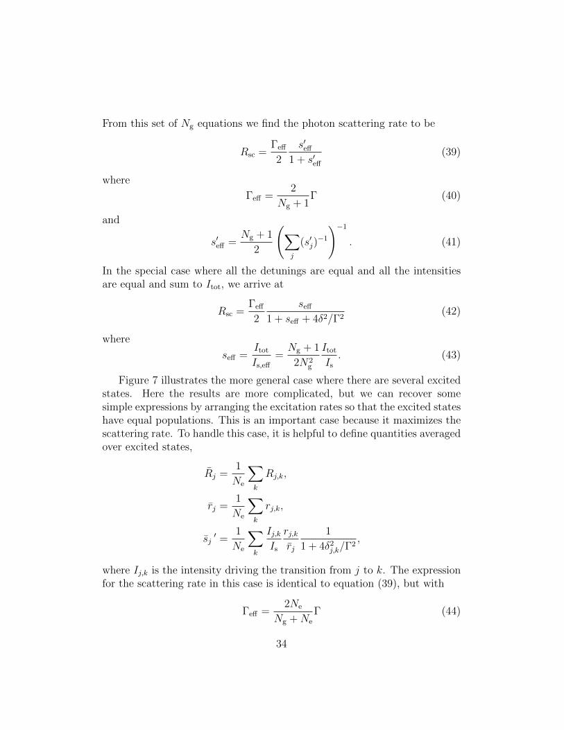
From this set of Ng equations we find the photon scattering rate to be

Rsc =Γeff

2

s′eff

1 + s′eff

(39)

where

Γeff =2

Ng + 1Γ (40)

and

s′eff =Ng + 1

2

(∑j

(s′j)−1

)−1

. (41)

In the special case where all the detunings are equal and all the intensitiesare equal and sum to Itot, we arrive at

Rsc =Γeff

2

seff

1 + seff + 4δ2/Γ2(42)

where

seff =Itot

Is,eff

=Ng + 1

2N2g

Itot

Is

. (43)

Figure 7 illustrates the more general case where there are several excitedstates. Here the results are more complicated, but we can recover somesimple expressions by arranging the excitation rates so that the excited stateshave equal populations. This is an important case because it maximizes thescattering rate. To handle this case, it is helpful to define quantities averagedover excited states,

Rj =1

Ne

∑k

Rj,k,

rj =1

Ne

∑k

rj,k,

sj′ =

1

Ne

∑k

Ij,kIs

rj,krj

1

1 + 4δ2j,k/Γ

2,

where Ij,k is the intensity driving the transition from j to k. The expressionfor the scattering rate in this case is identical to equation (39), but with

Γeff =2Ne

Ng +Ne

Γ (44)

34

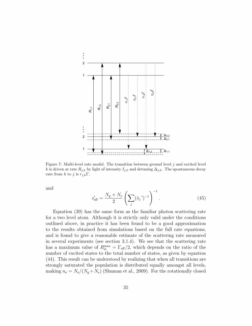
R1,1

R1,2

R2,1

R2,2 r 1,1Γ

r 2,1Γ

r 1,2Γ

r 2,2Γ

Δ1,1Δ1,2

Δ2,1Δ2,2

1

2

1

2

Figure 7: Multi-level rate model. The transition between ground level j and excited levelk is driven at rate Rj,k by light of intensity Ij,k and detuning ∆j,k. The spontaneous decayrate from k to j is rj,kΓ.

and

s′eff =Ng +Ne

2

(∑j

(sj′)−1

)−1

. (45)

Equation (39) has the same form as the familiar photon scattering ratefor a two level atom. Although it is strictly only valid under the conditionsoutlined above, in practice it has been found to be a good approximationto the results obtained from simulations based on the full rate equations,and is found to give a reasonable estimate of the scattering rate measuredin several experiments (see section 3.1.4). We see that the scattering ratehas a maximum value of Rmax

sc = Γeff/2, which depends on the ratio of thenumber of excited states to the total number of states, as given by equation(44). This result can be understood by realizing that when all transitions arestrongly saturated the population is distributed equally amongst all levels,making ne = Ne/(Ng +Ne) (Shuman et al., 2009). For the rotationally closed

35

transition discussed in section 2.5, the degeneracy of the ground state is threetimes that of the excited state, implying Rmax

sc = Γ/4 in the best case. Thisshows that the scattering rate, and associated force, will always be at leasttwo times smaller for a molecule than for a two-level atom with an identicallinewidth. In practice, it is common for the v = 1 repump laser to couple tothe same excited state as the main cooling laser, doubling Ng and reducingRmax

sc to Γ/7. In cases where there are small leaks to other rotational states,requiring microwave remixing (Yeo et al., 2015; Norrgard et al., 2016), Ng iseven larger and the maximum scattering rate is reduced even further. Theuse of more than one excited electronic state in the laser cooling scheme canbe a useful way to increase the scattering force. This method has been usedfor laser slowing of CaF where both the A2Π1/2 and B2Σ+ excited states wereused (Truppe et al., 2017a).

The scattering rate reaches half its maximum value when s′eff = 1. Inthe case of a single excited state, the laser intensity needed to reach thiscondition is Itot = 2N2

g/(Ng + 1)Is. Since there are always several groundstates, this intensity is considerably higher than the equivalent atomic case.We see from equation (45) that the individual s′j are summed in parallel ins′eff . If one of the set of sj is significantly smaller than all the rest, eitherbecause the Ij,k are too small or the δj,k are too large, that level becomesa bottleneck, limiting the value of seff and therefore Rsc. This shows theimportance of ensuring all ground states are coupled to at least one of theexcited states at an adequate rate.

To summarize, we see that in many cases of practical interest the max-imum photon scattering rate is reduced compared to the case of an idealtwo-level atom, that high laser intensity is needed to approach that maxi-mum rate, and that a single level excited at a smaller rate than all the otherscan greatly reduce the overall scattering rate. Figure 8 compares the reso-nant scattering rate achievable in typical atom cooling and molecule coolingexperiments. Atomic experiments often approximate the ideal two-level sys-tem where Rsc tends towards Γ/2 and the total intensity required is only afew times Is. For the molecular case, we use the rate equations to model aCaF molecule in a six-beam MOT where the levels of X2Σ+(v = 0, 1, N = 1)are driven to A2Π1/2(v′ = 0, J ′ = 1/2). The total intensity is divided equallybetween 8 frequency components which address the 8 hyperfine levels, all atzero detuning. The maximum rate is Rmax

sc = 0.13Γ, about 4 times smallerthan the atomic case, and the total intensity needed to reach a certain frac-tion of Rmax

sc is 28 times higher for the molecule than for the atom.

36

(i)

(ii)

0 20 40 60 80 100

0.0

0.1

0.2

0.3

0.4

0.5

Itot / Is

Rsc

/Γ

Figure 8: Photon scattering rate as a function of total intensity for two situations. (i)A two-level atom driven on resonance. (ii) A CaF molecule with all levels of X2Σ+(v =0, 1, N = 1) driven on resonance to A2Π1/2(v′ = 0, J ′ = 1/2). Dashed lines are the highintensity limits.

3.1.2. Force, damping constant and spring constant

In the context of a rate model, the motion of a molecule interacting with aset of laser beams is found by solving equation (36) together with equations(34). Approximate expressions for the scattering force for a set of beamscan also be obtained from the approximate expressions for the scatteringrate, most straightforwardly from equation (42). Because Rsc is not linearin intensity, the scattering rate due to one beam is altered by the presenceof other beams. An ad hoc approach to handling this is to argue that thescattering rate due to a particular beam should have the intensity of thatbeam in the numerator of equation (42), but have the total intensity of allbeams in the denominator so that the rate saturates in the right way (Lettet al., 1989). In this spirit, when there are Nb beams of equal intensity, the

scattering force due to beam i whose wavevector is ~ki can be written as

~Fi ≈~~kiΓeff

2

seff/Nb

1 + seff + 4(∆− ~ki · ~v)2/Γ2, (46)

where seff is the effective saturation parameter corresponding to the totalintensity of all Nb beams.

If two of the beams counter-propagate along x, so that ~k1 = −~k2 = kx,and all the others are orthogonal, the total force in the x-direction is Fx =

37

~F1 + ~F2. Using a Taylor expansion for small v, this is Fx = −αvx, where

α = −Γeff

Γ

8~k2(∆/Γ)(seff/Nb)

(1 + seff + 4∆2/Γ2)2. (47)

is the damping coefficient.A similar approach can be used to estimate the restoring force in a MOT,

where the counter-propagating beams have opposite handedness and themagnetic field at x is Ax for some constant A . In a simple picture ofthe MOT, the transitions driven by the beams with wavevectors ±kx areZeeman shifted by the angular frequencies ±∆ωZ = ±µeffAx/~, where µeff

is a characteristic magnetic moment. This changes ∆ to ∆ ∓ ∆ωZ in theexpression for the force due to each beam, equation (46). Using a Taylorexpansion for small x, the restoring force along x is Fx = −κx where

κ = −Γeff

Γ

8kµeffA(∆/Γ)(seff/Nb)

(1 + seff + 4∆2/Γ2)2(48)

is the spring constant.

3.1.3. Temperature

We can find an expression for the temperature following a standard ar-gument. We take the typical three-dimensional case where there are Nb = 6beams and consider the low velocity limit. Each photon scattering eventinvolves two randomly directed momentum kicks of size ~k, one due toabsorption and the other due to spontaneous emission. This is a randomwalk process, resulting in the mean square momentum increasing by δ〈p2〉 =2Rδt(~k)2 in a time δt. The rate of increase of energy for a molecule of massm is

Pheat =1

2m

δ〈p2〉δt

=Rsc~2k2

m.

The damping force is ~F = −α~v and the corresponding cooling power is

Pcool = ~F · ~v = −αv2 = −2αE

m,

where E is the kinetic energy. At equilibrium, Pheat + Pcool = 0. We equatethe equilibrium energy to 3/2kBTD, giving the Doppler temperature,

TD =~2k2

3

Rsc

kBα. (49)

38

Comparing equations (33) and (49) we see that, within this model, the dif-fusion constant is

D =~2k2Rsc

3. (50)

Equation (49) can be used to find the Doppler temperature along withany method for determining the scattering rate and damping constant, eitheranalytical or numerical. In the simplest approach, we can use equations (42)and (47) for Rsc and α, giving the result

TD = − ~Γ2

8kB∆(1 + seff + 4∆2/Γ2) (51)

for negative ∆. This is the same result as for a two-level atom. The minimumtemperature is obtained when ∆ = −1

2Γ√

1 + seff and is

TD,min =~Γ

2kB

√1 + seff . (52)

3.1.4. Applications of the rate model

The rate model gives a good estimate of the photon scattering rate in caseswhere dark states are destabilised at a rate close to or exceeding the scatteringrate (see section 2.7.1). This is the typical situation for laser slowing andmagneto-optical trapping. For SrF molecules, the scattering rates measuredin an rf MOT and a dc MOT (see section 5) agree reasonably well with thepredictions of the complete rate model and with the approximate result ofequation (42) (Norrgard et al., 2016). For CaF in a dc MOT, the measuredscattering rate was found to follow equation (42) but with Γeff about half thevalue given by equation (44), while the approximate analytical results for Rsc

were found to agree well with the full numerical results over a wide range ofintensities (Williams et al., 2017).

The trapping forces in a MOT are also described well by the rate model.For example, measurements of the spring constant as a function of scatteringrate in an rf MOT of SrF were found to fit well to the form of equation(48) re-expressed in terms of Rsc (Norrgard et al., 2016). For a dc MOTof CaF, the measured spring constant was found to be in good agreementwith the numerical results of the rate model, differing by less that 40% formeasurements spanning two orders of magnitude in intensity (Williams et al.,2017). Those results also fit well to equation (48) with Is,eff and µeffΓeff

treated as free parameters.

39

3.1.5. Limitations of the rate model

In most situations, the rate model fails to describe either the dampingconstant or the temperature. In the molecule MOTs studied so far, dampingconstants are typically an order of magnitude smaller than predicted by eitherequation (47) or numerical results of the rate model. Temperatures in a MOTare often an order of magnitude higher than given by equation (49) or (51)and show a much stronger dependence on intensity than suggested by thoseequations. In an optical molasses, with suitably chosen parameters, tem-peratures far below TD are obtained. These departures from the rate modelresults are all due to strong Sisyphus-type forces which often overwhelm theDoppler cooling forces, especially in the low velocity regime where dampingconstants and temperatures are typically measured. The proper descriptionof these forces requires a model based on the optical Bloch equations.

3.2. Optical Bloch equations

The use of optical Bloch equations to model the motion of atoms in laserfields was first developed by Gordon and Ashkin (1980) and later extendedto multi-level atoms by Ungar et al. (1989). These methods were recentlyextended to molecules and to three-dimensional light fields by Devlin andTarbutt (2016, 2018).

3.2.1. The model

The Hamiltonian of the system is

H = Hfield +Hmol +Hint (53)

where

Hfield =1

2

∫ (ε0 ~E

2 +1

µ0

~B2

)dV, (54)

Hmol =~P 2

2m+∑n

~ωn|n〉〈n|, (55)

Hint = −~µ · ~B − ~d · ~E. (56)

Here, ~E and ~B are the electric and magnetic field operators, ~d and ~µ arethe electric and magnetic dipole moment operators, ~P is the momentumoperator, ~ωn is the energy of state n and the sum runs over all relevantinternal states of the molecule. It is convenient to use the notation |g, j〉 and

40

|e, k〉 to distinguish levels of the electronic ground and excited states, with jand k representing all quantum numbers needed to identify each state. Wealso introduce the classical electric field of the light ~E ′.

The optical Bloch equations (OBEs) are obtained from the Heisenbergequation of motion

dA

dt= − i

~[A,H] (57)

applied to the molecular operators |g, j〉〈e, k|, |e, k〉〈e, k′| and |g, j〉〈g, j′|. The

commutator with Hint is evaluated by expanding ~d as

~d =∑j,k

~dj,k|g, j〉〈e, k|+ h.c. (58)

where~dj,k = 〈g, j|~d|e, k〉 (59)

and h.c. stands for the hermitian conjugate. The magnetic moment canbe expanded in a similar way. Spontaneous emission is introduced usingthe radiation reaction approximation in which the total electric field is thesum of the applied electric field of the light and a reaction field ~ERR =

16πε0c3

d3

dt3~d (Ungar et al., 1989). The resulting equations are given in Devlin

and Tarbutt (2016) for the case where the ground and excited states eachhave a single hyperfine level, and in Devlin and Tarbutt (2018) where thereare multiple hyperfine levels.

The force is

~F =d~P

dt= − i

~[~P ,H] = −~∇H. (60)

In the second step we have used equation (57), and in the third step we haveused the fact that H can be written in powers of the coordinates xi andmomenta pi, and the general result that [pi, g(~x)] = −i~ ∂g/∂xi for any g(~x)that can be expanded in powers of xi. The force due to the direct interactionwith a small applied magnetic field can often be neglected in comparison tothe much larger force exerted by the light field. In that case the expectationvalue of the force can be written in terms of ~∇(~dj,k · ~E ′) and expectation valuesof the molecular operators, 〈|g, j〉〈e, k|〉. The latter are found by solving theOBEs for a molecule dragged at constant velocity through the light field. In1D, depending on the polarization configuration, the solutions either reacha steady state or a quasi steady state where they become periodic with thesame periodicity as the Hamiltonian. In 3D, the Hamiltonian is periodic

41

along certain directions and it is convenient to solve for motion along thosedirections. After initial transients have decayed away, the expectation valueof the force becomes periodic and averaging over this period, and over aset of initial positions, gives the force along that direction. Repeating thisprocedure for many different velocities produces a velocity-dependent forcecurve.

We also need to determine the diffusion coefficient, which is (Cohen-Tannoudji, 1992)

Di = Re

∫ t

−∞dτ (〈Fi(τ)Fi(t)〉 − 〈Fi(τ)〉〈Fi(t)〉) , (61)

where i denotes the direction and ~F (t) is the force at time t. This involvesquantities of the form 〈(|g, j〉〈e, k|(τ))(|g, j〉〈e, k|(t))〉, the expectation valueof the product of molecular operators at two different times. This is notgiven directly by the OBEs, but for simple systems at rest can be related tothe solutions of the OBEs using the quantum regression method describedby Gordon and Ashkin (1980) and Mølmer (1991). Calculations of D(v) fora molecule moving through a 3D light field have not yet been attempted.However, numerical results for D(v) for various F → F ′ systems in 1D lightfields can be found in Chang and Minogin (2002) and could potentially beused to approximate molecules in 3D light fields. Alternatively, and moresimply, equation (50) can be used as a lower limit to the diffusion constant.

3.2.2. Sisyphus forces in 1D

There are two variations of the Sisyphus force for molecules, both utilizingdark states. They differ according to the mechanism that takes the moleculeout of the dark state - either motion through a changing polarization, or amagnetic field.

Figure 9 illustrates the first mechanism, in which the motion of themolecule through a changing polarization takes it from a dark to a brightstate. The method was described by Weidemuller et al. (1994) in the contextof cooling atoms below the recoil limit, and our description closely followsthe one given there. We consider a molecule with an F = 1 ground stateand an F ′ = 1 excited state. The transition dipole moment between mF = 1and m′F = 0 is dge. The molecule interacts with a pair of laser beams ofwavelength λ = 2π/k, counter propagating along z and linearly polarizedat an angle ±φ/2 to the x-axis. We call this the lin-φ-lin configuration. It

42

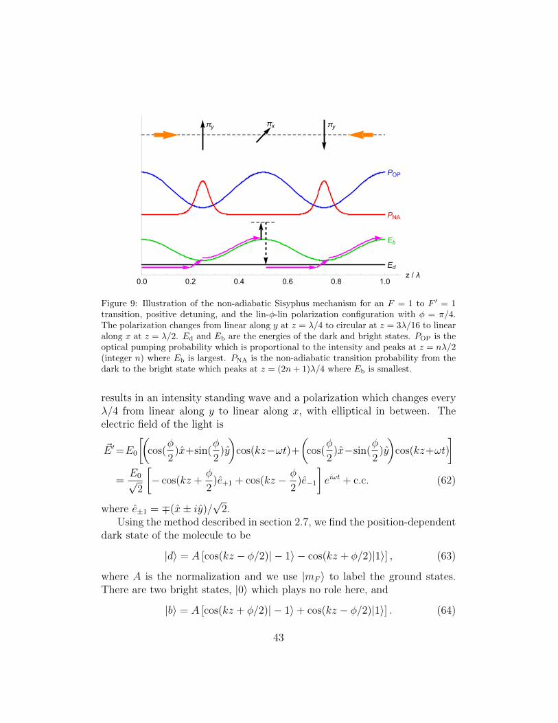
Ed

Eb

PNA

POP

πy πx πy

0.0 0.2 0.4 0.6 0.8 1.0z / λ

Figure 9: Illustration of the non-adiabatic Sisyphus mechanism for an F = 1 to F ′ = 1transition, positive detuning, and the lin-φ-lin polarization configuration with φ = π/4.The polarization changes from linear along y at z = λ/4 to circular at z = 3λ/16 to linearalong x at z = λ/2. Ed and Eb are the energies of the dark and bright states. POP is theoptical pumping probability which is proportional to the intensity and peaks at z = nλ/2(integer n) where Eb is largest. PNA is the non-adiabatic transition probability from thedark to the bright state which peaks at z = (2n+ 1)λ/4 where Eb is smallest.

results in an intensity standing wave and a polarization which changes everyλ/4 from linear along y to linear along x, with elliptical in between. Theelectric field of the light is

~E ′=E0

[(cos(

φ

2)x+sin(

φ

2)y

)cos(kz−ωt)+

(cos(

φ

2)x−sin(

φ

2)y

)cos(kz+ωt)

]=E0√

2

[− cos(kz +

φ

2)e+1 + cos(kz − φ

2)e−1

]eiωt + c.c. (62)

where e±1 = ∓(x± iy)/√

2.Using the method described in section 2.7, we find the position-dependent

dark state of the molecule to be

|d〉 = A [cos(kz − φ/2)| − 1〉 − cos(kz + φ/2)|1〉] , (63)

where A is the normalization and we use |mF 〉 to label the ground states.There are two bright states, |0〉 which plays no role here, and

|b〉 = A [cos(kz + φ/2)| − 1〉+ cos(kz − φ/2)|1〉] . (64)

43

The energy of the dark state is Ed = 0 and the energy of the bright state,which is its ac Stark shift, is

Eb =~∆

2

(−1 +

√1 +

2Ω2

∆2(1 + cos(2kz) cos(φ))

)≈ ~Ω2

2∆(1+cos(2kz) cos(φ)),

(65)where the approximation holds when Ω ∆. Here, ∆ is the detuning andΩ = dgeE0/~ is the Rabi frequency. Eb is positive when ∆ is positive, whichis the case illustrated in figure 9 and described below.

A molecule in a bright state will be optically pumped to the dark statewith a probability proportional to the intensity of the light field. This proba-bility is plotted in figure 9 and we see that it is largest when Eb is largest. Astationary molecule will remain in the dark state, but a molecule with speedv can make a non-adiabatic transition to the bright state with a probabilityPNA = |~v〈d| d

dz|b〉/Eb|2 (Messiah, 2014). Note that there is no transition

probability from |d〉 to |0〉, which is why |0〉 plays no role. Using equations(64) and (65) we obtain

PNA =sin2 φ

(1 + cosφ cos(2kz))4

(2∆

Ω

)2(kv

Ω

)2

. (66)

Figure 9 illustrates how PNA varies with z when φ = π/4, showing that it isstrongly peaked near the regions where Eb is smallest. Since transitions to|b〉 mainly happen at the bottom of the potential hill and transitions to |d〉mainly happen at the top, molecules repeatedly climb potential hills and loseenergy. This is the non-adiabatic Sisyphus mechanism which cools moleculeswhen ∆ > 0 and heats them when ∆ < 0.

The second Sisyphus mechanism is similar to the first but does not requirepolarization gradients. Instead, a magnetic field couples the dark and brightstates. We consider the same 1D situation described above with both beamspolarized along x (i.e. φ = 0), producing a standing wave of intensity withuniform polarization. The dark and bright states are simply |d〉 = 1√

2(| −

1〉− |1〉) and |b〉 = 1√2(|− 1〉+ |1〉). The energy of the bright state, Eb = ~ωb

is given by equation (65). In a magnetic field ~B = Bz, the | ± 1〉 stateshave a Zeeman shift of ±~ωZ = ±gFµBB. In the basis of |d〉 and |b〉 theHamiltonian is

H = ~(

0 −ωZ

−ωZ ωb

). (67)

44

(a)

-4 -2 0 2 4

-6

-4

-2

0

2

4

6

Velocity (Γ / k)

Force

(10-3ℏkΓ)

(b)

-0.10 -0.05 0.00 0.05 0.10

-6

-4

-2

0

2

4

6

Velocity (Γ / k)

Force

(10-3ℏkΓ)

Figure 10: Force versus velocity for a molecule with ground state F = 1 and excited stateF ′ = 1 interacting with light in the 1D lin-φ-lin polarization configuration discussed in thetext. Parameters are φ = π/4, ∆ = −2.5Γ, Ω = Γ/2, B = 0. (a) shows a wide velocityrange and (b) a narrow one. Modified from Devlin and Tarbutt (2016).

Consider a stationary molecule that is in the dark state at time t = 0.The probability of being in the bright state at time t is

Pb(t) =1

1 + η2sin2(

√1 + η2 ωZt) (68)

where η = ωb/(2ωZ). When Ω ∆ we can use the approximate form of Eb

in equation (65), giving η ≈ ηmax cos2(kz) where ηmax = Ω2/(2∆gFµBB). Wefocus on the case where ηmax 1. Away from the nodes of the standing wave,the probability of being in the bright state is always very small and oscillatesat high frequency, while at the nodes the probability oscillates between 0and 1 at angular frequency ωZ. For a moving molecule the Hamiltonianin equation (67) is time-dependent and the Schrodinger equation has to besolved numerically, but for a slowly-moving molecule the picture is the sameas already described – the molecule is highly likely to remain in the dark stateexcept when it passes through the nodes where it has a high probability oftransferring to the bright state. This results in exactly the same picture ofSisyphus cooling as in figure 9, and is sometimes called the magnetically-assisted Sisyphus effect. It was first elucidated in the context of sub-Dopplercooling of atoms (Emile et al., 1993; Sheehy et al., 1990), and was described

45

in the very first work on laser cooling of molecules where it was found to bean effective cooling mechanism (Shuman et al., 2010).

Figure 10 shows an example of the force obtained from the solutions tothe optical Bloch equations for an F = 1 to F ′ = 1 system. In this example,φ = π/4 and B = 0, so the force at low velocity is due to the non-adiabaticSisyphus effect. Because the detuning is negative, this force results in strongheating. Reversing the detuning reverses the sign of the force. The maximumSisyphus force in this system is similar in magnitude to the sub-Dopplercooling forces obtained in type-I systems (i.e. when F ′ > F ) at these valuesof Ω and ∆. At higher speeds, v > 0.2Γ/k, there is a damping force in thisconfiguration, but this is about 100 times weaker than the Doppler coolingforce in a type-I system. The equivalent force curves for the magnetically-assisted Sisyphus effect are very similar to the ones shown in figure 10, andcan be found in Emile et al. (1993).

3.2.3. Sisyphus forces in 3D

In a three-dimensional light field there are always intensity gradients andpolarization gradients. As a result, the non-adiabatic Sisyphus force out-lined above plays a central role in laser cooling of type-II systems. Themagnetically-assisted Sisyphus effect can also be important in 3D if a mag-netic field of a suitable size is applied, typically in the range 0.1 G to a fewG.

In 3D, the force has components both parallel and perpendicular to thevelocity. Although the perpendicular components can be significant (Devlinand Tarbutt, 2016), especially at low speeds, we focus here on the paral-lel component, which has been explored in much more detail. Figure 11shows these parallel forces for two standard 3D polarization configurations,the σ+σ− configuration and the lin-⊥-lin configuration, and compares theresults for a type-II system (F = 1 → F ′ = 1) to those for a type-I sys-tem (F = 1 → F ′ = 2). Here, the detuning is negative. The results in3D for the type-I system are very similar to their 1D counterparts and canbe interpreted in terms of well known 1D models of sub-Doppler cooling -the Sisyphus effect for the lin-⊥-lin configuration and orientational coolingfor σ+σ− (Dalibard and Cohen-Tannoudji, 1989; Ungar et al., 1989). Thesepolarization gradient forces have the same sign as the Doppler cooling forceand provide much stronger damping at low velocities, leading to tempera-tures below the Doppler limit. The results in 3D for the F = 1 → F ′ = 1system are quite different to the 1D case. In fact, for these two polariza-

46

0.0 0.2 0.4 0.6 0.8 1.04

2

0

2

4

6

0.0 0.2 0.4 0.6 0.8 1.0

4202468

Speed (Г/k)

Forc

e (1

0-3 ћ

kГ)

lin lin

σ+σ-

0.0 0.2 0.4 0.6 0.8 1.0

1

0

1

2

3

Forc

e (1

0-3 ћ

kГ)

lin lin

σ+σ-

Speed (Г/k)

c) F = 1 → F΄ = 0

b) F = 1 → F΄= 1

Speed (Г/k)

Forc

e (1

0-3 ћ

kГ)

d) F = 2 → F΄= 1

σ+σ-

lin lin

0.0 0.2 0.4 0.6 0.8 1.020

15

10

5

0

Speed (Г/k)

Forc

e (1

0-3 ћ

kГ)

lin lin

σ+σ-

a) F = 1 → F΄= 2

Figure 11: Force in the direction of the velocity, plotted as a function of velocity, for twodifferent 3D polarization configurations and two different systems. a) F = 1→ F ′ = 2, b)F = 1 → F ′ = 1. Parameters are ∆ = −2.5Γ, Ω = Γ/2, B = 0. The widths of the linesshow the 68% confidence intervals on the mean force. Modified from Devlin and Tarbutt(2016).

tion configurations, the force is zero at all velocities in 1D, while in 3D theforce is large, similar in magnitude to the type-I case. In type-II systems theSisyphus-type force, which dominates at low velocity, has the opposite signto the Doppler cooling force which dominates at high velocity and the dom-inance of the Sisyphus force extends to a higher velocity than in the type-Isystems. This leads to a zero crossing of the force at a critical velocity, vc,whose value is far greater than the mean velocity at the Doppler limit, evenat modest intensities. For negative detuning, the force drives the moleculestowards vc and this high equilibrium speed leads to the high temperaturesfound in magneto-optical traps of type-II systems. Unlike type-I systemswhere polarization gradient forces are inhibited by a magnetic field, the Sisy-phus forces in type-II systems persist over the whole range of magnetic fieldstypically seen by molecules in a MOT (Devlin and Tarbutt, 2018). The crit-ical velocity is found to be independent of detuning and proportional to thesquare root of the laser intensity (Devlin and Tarbutt, 2016). This is consis-tent with the observation that the temperature in molecular MOTs increaseswith increasing laser intensity (Norrgard et al., 2016; Truppe et al., 2017b;Williams et al., 2017; Anderegg et al., 2017).

For positive detuning, molecules with speeds above vc are accelerated tohigh speed, while those below vc are strongly damped towards zero velocity.As can be seen from the illustration in figure 9, slow-moving molecules spend

47

-4

-2

0

2

4

Acceleration(103m/s2)

-6

-4

-2

0

2

0

10

20

30

40

50

60

70

Excitedfraction(10-3)

0

10

20

30

40

50

60

70

0 1 2 3 4 5 6 7 80

10

20

30

40

50

Speed (m/s)

v2W(v)(s/m

)

0 1 2 3 4 5 6 7 80.00

0.01

0.02

0.03

0.04

Speed (m/s)

(i) (ii)

Figure 12: Acceleration, excited-state fraction and probability density versus speed forCaF molecules in two situations. (i) Optical molasses. Intensity of cooling light is456 mW/cm2 and detuning is 2.61Γ. (ii) Centre of MOT. Intensity of cooling light is234 mW/cm2 and detuning is −0.64Γ. Modified from Devlin and Tarbutt (2018).

much of their time in dark states, so the photon scattering rate is low. Thiscombination of a low heating rate and strong damping can lead to very lowtemperatures, as described in section 6.

3.2.4. Applications of the OBE model

OBE models have been used to simulate experiments demonstrating one-dimensional transverse cooling of YbF (Lim et al., 2018) and YbOH (Augen-braun et al., 2020c) beams and to estimate the scattering rate for transversecooling of BaH (McNally et al., 2020). For YbF, the spatial distributionsdetermined using the FPK equation are in fairly good agreement with mea-surements. For YbOH, the force curves generated by solving the OBEs were

48

used for trajectory simulations of a set of molecules. These simulations in-clude random decays to dark vibrational levels and the random momentumdiffusion due to photon recoil. The simulated beam profiles generated thisway agree well with the measured ones, and the simulations are accurate inpredicting how the beam width and fraction of ultracold molecules dependon the detuning and intensity. For both YbF and YbOH, the simulationspredict temperatures in the range 1-10 µK, which is below the temperatureresolution of the experiments.

In 3D, generalised optical Bloch equations have been used to calculatethe velocity-dependent force for CaF in an optical molasses, and the positiondependence and velocity dependence of the force in a MOT (Devlin andTarbutt, 2018). The OBEs also give the scattering rate as a function ofvelocity, which was used in equation (50) to estimate the diffusion constant.The resulting F (v) and D(v) were then used in the FPK equation in orderto determine velocity distributions, and to estimate how temperatures andother parameters depend on the various experimental parameters. Figure 12summarizes some key information obtained from these simulations. We seethat the force curves for the full molecular system are found to be similarto those for the model F = 1 → F ′ = 1 system presented in figure 11b).The fraction of molecules in the excited state is smaller than predicted bya rate model at all speeds, and is in good agreement with measured values.The excited-state population drops at low speed due to optical pumping intotransient dark states, though does not go to zero at zero velocity. This showsthat motion through the light field is an important factor in de-stabilizingdark states, though not the only factor.

In the molasses, where the light is blue-detuned (figure 12(i)), the velocitydistribution is close to a thermal distribution. The modelling predicts adamping time in the molasses of about 100 µs, close to the measured value,but the predicted temperature is 3-6 times lower than measured over a widerange of parameters, indicating that the fluctuating dipole force, which isneglected in the model, is a major source of heating in the optical molasses.The predicted temperature dependence on intensity, detuning and magneticfield were all found to be similar to the measured trends. In the MOT, wherethe light is red-detuned (figure 12(ii)), the velocity distribution peaks nearthe velocity where the force crosses zero. The distribution is determinedby a balance between Doppler cooling and Sisyphus heating. Although thedistribution is far from thermal, the ballistic expansion of molecules with thisdistribution looks similar to that of a thermal distribution. The temperatures

49

determined this way depend on the intensity, and are similar to the measuredvalues.

OBE simulations have also proven useful in designing deep laser coolingschemes that cool molecules towards the recoil limit (Cheuk et al., 2018;Caldwell et al., 2019). These methods typically rely on the combinationof strong Sisyphus cooling to damp the velocity towards zero, and opticalpumping into robust dark states so that stationary molecules do not scat-ter photons. In Caldwell et al. (2019) two deep laser cooling schemes aremodelled and compared to experiment. For one scheme, the model suggeststhat it is feasible to cool below the recoil limit, although this has yet to beachieved and the simulation method breaks down in that limit.

3.2.5. Limitations of the OBE model

As described in section 3.2.1, the force is obtained by finding the quasisteady state solutions of the OBEs for a molecule dragged at constant velocitythrough the light field. The accuracy of this method is questionable sinceit ignores the transient response of the molecule. It takes many photonscattering events for the transient to diminish, and in that time the force maychange the speed appreciably, while the momentum diffusion may randomiseit. Nevertheless, for speeds v & 0.2

√~Γ/m, the method is found to agree

quite well with the force obtained from Monte Carlo simulations that includea random walk to simulate the momentum diffusion (Ungar et al., 1989). Thismeans that we might expect the method to work well for temperatures downto about 0.2TD,min, but to be inaccurate at lower velocities. The method alsotreats the motion of the molecule classically, so must break down once thetemperature approaches the recoil limit.

Another significant limitation of the model is the difficulty of accuratelydetermining the diffusion constant. While methods exist to evaluate D(v) insome cases (Gordon and Ashkin, 1980; Mølmer, 1991; Agarwal and Mølmer,1993), they have not yet been extended to the more complex situation of amolecule moving through a 3D light field. Without a proper evaluation ofD(v), the temperatures predicted by the model will not be accurate. Thedevelopment of methods to address this shortcoming would be particularlyvaluable.

50

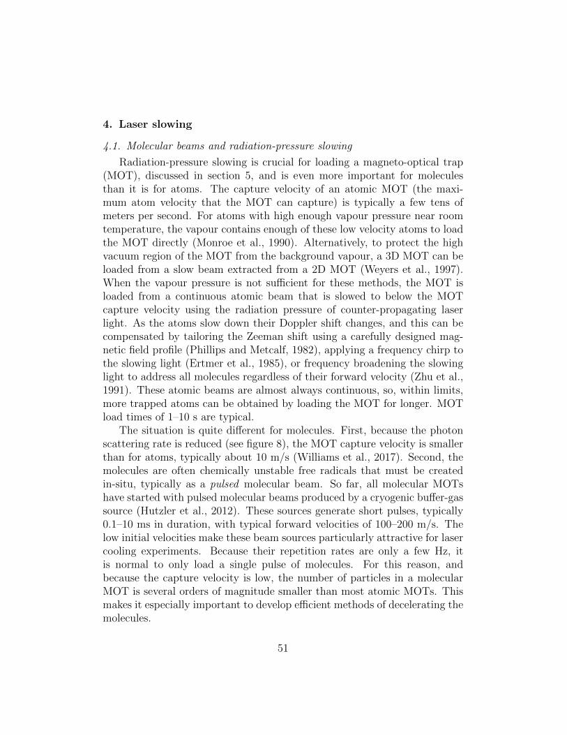
4. Laser slowing

4.1. Molecular beams and radiation-pressure slowing

Radiation-pressure slowing is crucial for loading a magneto-optical trap(MOT), discussed in section 5, and is even more important for moleculesthan it is for atoms. The capture velocity of an atomic MOT (the maxi-mum atom velocity that the MOT can capture) is typically a few tens ofmeters per second. For atoms with high enough vapour pressure near roomtemperature, the vapour contains enough of these low velocity atoms to loadthe MOT directly (Monroe et al., 1990). Alternatively, to protect the highvacuum region of the MOT from the background vapour, a 3D MOT can beloaded from a slow beam extracted from a 2D MOT (Weyers et al., 1997).When the vapour pressure is not sufficient for these methods, the MOT isloaded from a continuous atomic beam that is slowed to below the MOTcapture velocity using the radiation pressure of counter-propagating laserlight. As the atoms slow down their Doppler shift changes, and this can becompensated by tailoring the Zeeman shift using a carefully designed mag-netic field profile (Phillips and Metcalf, 1982), applying a frequency chirp tothe slowing light (Ertmer et al., 1985), or frequency broadening the slowinglight to address all molecules regardless of their forward velocity (Zhu et al.,1991). These atomic beams are almost always continuous, so, within limits,more trapped atoms can be obtained by loading the MOT for longer. MOTload times of 1–10 s are typical.

The situation is quite different for molecules. First, because the photonscattering rate is reduced (see figure 8), the MOT capture velocity is smallerthan for atoms, typically about 10 m/s (Williams et al., 2017). Second, themolecules are often chemically unstable free radicals that must be createdin-situ, typically as a pulsed molecular beam. So far, all molecular MOTshave started with pulsed molecular beams produced by a cryogenic buffer-gassource (Hutzler et al., 2012). These sources generate short pulses, typically0.1–10 ms in duration, with typical forward velocities of 100–200 m/s. Thelow initial velocities make these beam sources particularly attractive for lasercooling experiments. Because their repetition rates are only a few Hz, itis normal to only load a single pulse of molecules. For this reason, andbecause the capture velocity is low, the number of particles in a molecularMOT is several orders of magnitude smaller than most atomic MOTs. Thismakes it especially important to develop efficient methods of decelerating themolecules.

51

To date, all molecular MOT experiments have used frequency-chirpedor frequency-broadened laser slowing methods. For typical speeds of 100–200 m/s, and a cycling transition at a visible wavelength, the required fre-quency range of the chirp or broadening is a few hundred MHz. With scat-tering rates of around 106 photons/second, the acceleration is about 104 m/s2

and the molecules will come to rest in about 10 ms after scattering around104 photons. Rapid destabilization of dark states is important for efficientslowing and can be done using a magnetic field or polarization modulation(see section 2.7). The first radiation pressure slowing of a molecular beamwas demonstrated by Barry et al. (2012). Starting from a SrF beam with amean speed of 140 m/s, about 6% of the molecules were decelerated to speedsbelow 50 m/s. The frequency spectrum of the laser was broadened to a fewhundred MHz to implement the frequency broadened slowing method. Usingthis method, the final velocity is determined by the frequency spread andaverage detuning of the light, and the duration of the slowing. In frequency-chirped slowing (Zhelyazkova et al., 2014; Truppe et al., 2017a), the finalbeam velocity is determined by the initial detuning, the chirp rate, and theduration of the slowing period. We note that some experiments use a com-bination of frequency-broadened and frequency-chirped slowing (Yeo et al.,2015).

The slowing method should bring as many molecules as possible into thecapture volume and capture velocity of the MOT. This is challenging, be-cause the initial distribution from the molecular source is often broad invelocity, position, and time. Without any transverse cooling, slow moleculesdiverge rapidly, so ideally all molecules would reach the target velocity justas they reach the MOT. In practice, laser slowing tends to bring molecules toa particular forward velocity at a particular time, and the beam often has awide spread of axial positions at that time. Those molecules that are still farfrom the MOT will diverge too much and are unlikely to be captured. Moremolecules could be captured if the slowing procedure naturally brought themto the desired forward velocity at a specific position. That happens in theZeeman slowers commonly employed in cold atom experiments (Phillips andMetcalf, 1982), and the development of Zeeman slowing for molecules is ongo-ing (Petzold et al., 2013; Liang et al., 2019). Quasi-continuous beams basedon high repetition rate molecular beams sources are also currently being de-veloped (Shaw and McCarron, 2020) and are likely to substantially increasethe number of molecules loaded, especially in combination with a Zeemanslower. Other ways to improve the efficiency of beam-to-MOT transfer are

52

discussed below.

4.2. Simulating the slowing sequence

Simulations are useful to evaluate the performance of a chosen slowingmethod, and to maximize the number of slow molecules loaded into theMOT as a function of the many variable parameters, e.g amount of frequencybroadening, chirp amplitude, chirp rate and functional form. Simulatingindividual molecule trajectories using a semi-classical Monte-Carlo approachbased on a rate-model has been found to accurately predict most observedslowing results (Truppe et al., 2017a; Williams et al., 2017). Coherencesappear to play little role in beam slowing, so the rate model is adequate.

Once the frequency spectrum and polarization of the light is fixed, thesteady-state scattering rate, Rsc = Γne, depends on only two parameters, adetuning δ and the total laser intensity I. In this reduced parameter space, itis computationally efficient to calculate Rsc for a large set of δ and I values,interpolate over these values to make a scattering rate map Rsc(δ, I), andthen use this map to simulate individual molecule trajectories. After calcu-lating the transition amplitudes between all magnetic sublevels of the groundand excited states for the chosen magnetic field and laser polarization, Rsc

is calculated by finding the steady-state solutions to equations (34). Thesteady-state solutions are sufficient because the populations reach the steadystate on a timescale much shorter than any changes in the slowing parame-ters. To account for population remixing amongst the magnetic sublevels byan applied magnetic field, an additional ad hoc term∑

j′

ωj − ωj′2π

(ngj − ngj′)δFF ′ (69)

is added to the right hand side of equation (34a). Here, ~ωj is the Zeemanshift of level j.

Simulating molecule trajectories begins by choosing a set of moleculeswith initial positions and velocities reflecting the characteristics of the molec-ular beam. Their trajectories are calculated as follows. At each time step dtthe probability of scattering a photon is P = Rscdt. The time step is chosenso that P 1. A random number, r, between 0 and 1 is chosen, and ifP > r a photon is scattered. In that case, the momentum in the direction ofthe laser’s k vector is increased by ~k to account for the absorption, and themomentum in a direction chosen at random from an isotropic distribution

53

is increased by ~k to account for spontaneous emission. The state distribu-tion of the molecules in the beam can be tracked by choosing the excitedand subsequent ground state according to a quasi-random sampling of theset of available paths weighted by the the relative transition dipole strengthsin excitation and the corresponding branching ratios in decay. In this way,slowing, stochastic heating, and the evolution of the internal degrees of free-dom are taken into account. The spatial profile of the slowing laser, overallintensity, initial detuning, and the time-dependence of any chirp, are all pa-rameters that can be optimized through these simulations and comparedto experiments. Many of these parameters can be explored and optimizedwithout re-calculating the scattering rate map.

4.3. Frequency chirped versus frequency broadened slowing

Which is most effective, frequency chirped slowing or frequency broad-ened slowing? This is an important question that simulations can help an-swer. Both approaches have been studied for CaF molecules, slowed using theB2Σ+(v′ = 0)−X2Σ+(v = 0) cycling transition (Truppe et al., 2017a). Someresults are illustrated in figure 13. For frequency-chirped slowing, shown infigure 13(a), frequency sidebands are added to the slowing light in order to ad-dress all hyperfine components rather than addressing molecules with manydifferent speeds. In this case, an EOM was used to generate the frequencysidebands shown. The initial overall detuning is chosen so that molecules nearthe peak of the velocity distribution (solid blue line) are Doppler shifted intoresonance. The overall chirp of the entire sideband structure is indicated bythe green arrow. In frequency-broadened slowing, shown in figure 13(b), thespectrum of the laser light is broadened over a wider range. The structureshown was generated by sequentially passing the slowing light through EOMsdriven at 74, 24, and 8 MHz. Example scattering rate maps correspondingto these two sideband structures are shown in figure 13(c) and (d).

Figure 14 compares the results of frequency chirped and frequency broad-ened slowing experiments for CaF molecules, with corresponding simula-tions (Truppe et al., 2017a). We see that frequency chirped slowing pro-vides significantly more axial cooling of the molecular beam. This is becausechirped slowing slows the faster molecules before the slower ones, which com-presses the axial velocity distribution. By contrast, frequency-broadenedslowing addresses most forward velocities present in the molecular beam atall times and does not produce significant cooling until the molecules are slowenough to fall out of resonance with the light. The higher level of control

54

0 50 100 150 200 250

0 - 100 - 200 - 300 - 400

Velocity (m/s)

Numberofmolecules

(arb.)

Detuning (MHz)

RelativelaserIntensity

0 50 100 150 200 250

0 - 100 - 200 - 300 - 400

Velocity (m/s)

Numberofmolecules

(arb.)

Detuning (MHz)

Relativelaserintensity

(a) (b)

(c) (d)

Rsc (106/s) Rsc (106/s)

1

2

3

4

5

Lase

r in

tensi

ty (

W/c

m2)

0

1

2

3

4

5

Lase

r in

tensi

ty (

W/c

m2)

0

Relative detuning (MHz)

-200 -100 0 100 200

Relative detuning (MHz)

-200 -100 0 100 200

Figure 13: Two general approaches for laser slowing. The blue curve(s) indicate a typicalinitial velocity distribution for a buffer-gas molecular beam. (a) In chirped-laser slowing,frequency sidebands are added to the slowing laser to address the hyperfine componentsof the transition. As the molecules slow down, the light is chirped towards resonance,indicated by the green arrow. (b) In frequency-broadened slowing, a fixed frequencyspectrum is broadened more significantly and detuned such that molecules stop scatteringphotons once the target velocity has been reached. (c,d) Examples of scattering ratemaps for laser slowing of CaF molecules on the B2Σ+ −X2Σ+ transition using the laserfrequency spectra shown in (a,b).

of the beam forward velocity, together with increased axial cooling, makesfrequency-chirped slowing more efficient at bringing molecules to the verylow velocities needed for loading a MOT, as shown in figure 14(c) and fig-ure 14(d). Chirped slowing is also a more efficient way to use the availablelaser power since, at all times, most of the power is at frequencies that areclose to resonance. On the other hand, frequency-broadened slowing is sig-nificantly simpler, with fewer control parameters and less sensitivity to theexact characteristics of the molecular beam. It may be the preferred methodwhen the distribution of forward velocities is large, or when the source-to-trap distance is too short for a chirp to be useful, or when the molecular

55

beam properties tend to vary in time.

4.4. Reducing losses during slowing

In current experiments, only a small fraction4 of the molecules producedby the source are captured in the MOT because the beam diverges as itis slowed. This divergence is exacerbated by the stochastic heating associ-ated with spontaneous emission (see section 3.1.3). Typically, the transversetemperature increases by a few mK, corresponding to an increase in thetransverse velocity spread of . 1 m/s. One way to reduce the transverse di-vergence slightly is to use a converging slowing laser, which has been shownto increase the number of molecules in the MOT by a factor of 2–3 (Stei-necker et al., 2016). A number of approaches are being pursued to moresignificantly reduce losses associated with beam divergence during slowing.Ideas include: (i) decelerate the beam so rapidly that it does not have timeto diverge; (ii) focus or guide the beam while it is being slowed; (iii) applytransverse cooling either before or during slowing to minimize beam diver-gence. All have the potential to increase the number of molecules in a MOTby a large factor.

The first option can work well for a light molecule that has a very strongtransition at a short wavelength, so that the scattering rate is high and thenumber of photons that have to be scattered is relatively low. The AlFmolecule is an interesting example, having a cycling transition at 228 nmwith a decay rate of 84 MHz (see table 1). Rapid deceleration can alsobe achieved using stimulated scattering processes (Chieda and Eyler, 2011;Ilinova et al., 2015; Kozyryev et al., 2018; Galica et al., 2018; Long et al.,2019; Wenz et al., 2020). These approaches can transfer momentum at ahigh rate and can even work for molecules that lack good cycling transitionssince they largely bypass spontaneous emission. However, the intensitiesavailable from current continuous wave lasers are probably not sufficient toproduce these strong forces over the large spatial area needed to slow typicalmolecular beams. Current work by Beyer et al. (2020) is seeking to fill thistechnological gap.

Option (ii), guiding while slowing, is an attractive option that could beachieved in several ways. For example, Fitch and Tarbutt (2016) have pro-

4The trajectory simulations discussed above for frequency-chirped or frequency-broadened slowing estimate that typically < 0.01% of the molecules that leave the buffer-gas source are captured in the MOT.

56

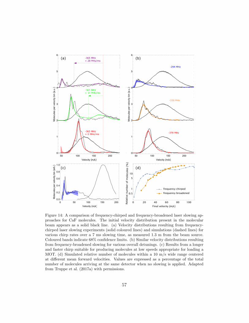
50 100 150 2000

1

2

3

4

5

6

Velocity (m/s)

Moleculespervelocitybin

(a.u.)

-365 MHz + 0 MHz/ms

-365 MHz+ 14 MHz/ms

-365 MHz+ 28 MHz/ms

50 100 150 2000

1

2

3

4

5

6

Velocity (m/s)

Moleculespervelocitybin

(a.u.)

-378 MHz

-336 MHz

-294 MHz

0 50 100 150 2000.0

0.2

0.4

0.6

0.8

1.0

Velocity (m/s)

Moleculespervelocitybin

(arb.)

(a) (b)

(c)

frequency chirpedfrequency broadened

0 20 40 60 80 100

0.51

510

Final velocity (m/s)

%of

totalunslowedmolecules

(d)

Rel

ativ

e num

ber

of m

olec

ule

s (%

)

Figure 14: A comparison of frequency-chirped and frequency-broadened laser slowing ap-proaches for CaF molecules. The initial velocity distribution present in the molecularbeam appears as a solid black line. (a) Velocity distributions resulting from frequency-chirped laser slowing experiments (solid coloured lines) and simulations (dashed lines) forvarious chirp rates over a 7 ms slowing time, as measured 1.3 m from the beam source.Coloured bands indicate 68% confidence limits. (b) Similar velocity distributions resultingfrom frequency-broadened slowing for various overall detunings. (c) Results from a longerand faster chirp suitable for producing molecules at low speeds appropriate for loading aMOT. (d) Simulated relative number of molecules within a 10 m/s wide range centeredat different mean forward velocities. Values are expressed as a percentage of the totalnumber of molecules arriving at the same detector when no slowing is applied. Adaptedfrom Truppe et al. (2017a) with permissions.

57

posed a magnet geometry where focusing stages alternate with strong-fieldstages, and optical pumping transfers molecules between weak- and strong-field seeking states, resulting in both guiding and deceleration. Since themagnetic field is used to remove kinetic energy, rather than laser photons,far fewer photons need to be scattered in order to slow the molecules down.As such, this technique may be particularly useful for molecules that lackhighly-closed cycling transitions. Another option, proposed by DeMille et al.(2017), is to use a microwave field blue detuned from a rotational transition inthe molecule to provide transverse confinement. Alternatively, laser-coolablemolecules are usually amenable to more established slowing methods suchas Stark (Bethlem et al., 1999; Osterwalder et al., 2010), Zeeman (Van-haecke et al., 2007; Narevicius et al., 2008; Lavert-Ofir et al., 2011), or cen-trifuge (Chervenkov et al., 2014) deceleration. All of these provide transverseguiding during slowing but typically select only a small fraction of the axialpositions and velocities in the molecular beam for deceleration to the targetvelocity. The combination of these slowing methods with laser cooling tech-niques (Wall et al., 2011) is an interesting avenue which, at present, remainslargely unexplored.

Option (iii), transverse cooling, is potentially very powerful since it pro-duces a highly collimated molecular beam that can then be slowed efficiently.Additionally, an electric or magnetic lens can be used to focus moleculesinto the laser cooling region in order to capture a larger fraction of the ini-tial transverse velocity distribution, resulting in an intense, slow, collimatedbeam (Fitch et al., 2020).

5. Magneto-optical trapping

The magneto-optical trap (MOT) (Raab et al., 1987) is the starting pointof almost all experiments that use ultracold atoms. The MOT cools andtraps atoms using pairs of counter-propagating laser beams, typically alongthree orthogonal axes, along with a magnetic field gradient to distinguishbetween the beams. In recent years, MOTs of SrF, CaF and YO moleculeshave been made (Barry et al., 2014; Truppe et al., 2017b; Anderegg et al.,2017; Collopy et al., 2018), and MOTs of several other molecular species arebeing developed. Magneto-optical traps can be classified according to thetotal angular momenta of the ground and excited states, F and F ′. In type-IMOTs, F ′ > F so there are no dark states, whereas in type-II MOTs F ′ ≤ Fso there are dark states in the system that play an important role. Type-II

58

Distance from centre

Energy

m'=-2,-1,0,1,2

m=1

m=0

m=-1

F=1

F'=2

(a)

Distance from centre

Energy

m'=1

m'=0

m'=-1

m=1m=0m=-1

F=1

F'=1

(b)

Figure 15: Level structures where MOTs fail. (a) No Zeeman splitting in the excited state.(b) F = 1→ F ′ = 1 in 1D.

atomic MOTs (Raab et al., 1987; Prentiss et al., 1988; Shang et al., 1994;Flemming et al., 1997; Nasyrov et al., 2001; Atutov et al., 2001; Tiwari et al.,2008) result in lower densities and higher temperatures than type-I MOTs, soare very rarely used. The closed cooling transitions in molecules are type-IItransitions (see section 2.5), so molecular MOTs are type-II MOTs. In thefollowing, we consider the nature of the cooling and trapping forces in theseMOTs and review the progress in producing them. As a reminder, we useF and F ′ to refer to the total angular momentum of the ground and excitedstates, g and g′ to refer to their magnetic moments, and ∆ to refer to thedetuning of the light from resonance. We use σ± to refer to polarizationsthat drive ∆m = ±1 transitions, and the term ‘restoring beam’ to refer tothe beam that pushes a displaced molecule back towards the centre. Unlessstated otherwise, the z-axis is in the direction of the magnetic field.

An analysis of MOTs for atoms or molecules with a single transitionF → F ′ driven by a single frequency of light brings out several useful in-sights (Tarbutt, 2015). (1) If there is no Zeeman splitting in the excitedstate (g′ = 0) there is no confining force. The confining forces in a MOTarise because the Zeeman splitting brings the atom closer to resonance withthe restoring beam. When g′ = 0, and for any m, the ∆m = ±1 transi-tions have the same detuning, so there is no net force. This is illustrated

59

in figure 15(a) and is true for any choice of F and F ′. (2) When g′ > 0and ∆ < 0, the restoring beams should be polarized to drive σ− transitionswhen F ′ ≥ F , and to drive σ+ transitions when F ′ < F . These polarizationrequirements are reversed when g′ < 0 or when ∆ > 0. The sign of g hasno influence on the required polarization. (3) In a one-dimensional MOTthere is no confining force when F = F ′ = 1. This case is illustrated infigure 15(b). When the atom is in m = 1 it is only bright to the beam thatdrives ∆m = −1 transitions, and when it is in m = −1 is is only bright to theopposing beam that drives ∆m = +1 transitions. In both cases the excitedstate is m′ = 0 which decays to m = ±1 with equal probability. It followsthat equal numbers of photons are scattered from the counter-propagatingbeams, so there is no net force. Although this result is special to this case, itillustrates the general problem of making MOTs when there are dark states -the atom quickly goes dark to the beam that would otherwise push it towardsthe centre. (4) In three dimensions the orthogonal beams play an importantrole in pumping molecules out of dark states, and a confining force can berecovered. Nevertheless, the presence of dark states results in substantiallysmaller forces than for type-I MOTs.

The first issue discussed above is particularly important for moleculeswith 2Π1/2 − 2Σ cooling transitions. A pure 2Π1/2 state has g′ ≈ 0 becausethe magnetic moments associated with the orbital and spin angular momentaare very nearly equal but opposite. Mixing of the 2Π1/2 state with nearbyΣ states results in a non-zero value of g′, but this is usually small. Withoutmitigation, the small value of g′ and the presence of dark states would resultin very weak confining forces. Fortunately, there are two good ways to avoidthese problems.

5.1. Dual-frequency MOT

The difficulties outlined above apply when there are isolated transitionsdriven by a single frequency of light. They can be avoided by using twofrequencies of opposite polarization. This scheme, introduced in Tarbuttand Steimle (2015), is known as a dual-frequency MOT or a dc MOT, andis illustrated in figure 16(a) for the particular case of an F = 2 groundstate and an F ′ = 1 excited state. Each MOT beam contains two frequencycomponents of opposite handedness, one red detuned and the other bluedetuned. The red detuned restoring beam drives σ− transitions, and theblue detuned one drives σ+ transitions. As always, the opposing beamsdrive the opposite transitions. A molecule in a state of positive m can only

60

+2+10-1-2

-1,0,+1

F=2

F'=1

δ1

δ2

σ-

σ+

σ+ σ+ σ+ σ-

X 2Σ+ (N=1)

F=1

F=0

F=1F=2

A 2Π1/2 (J=1/2) F'=0F'=1

(a) (b)

Figure 16: (a) Scheme for dual frequency MOT, illustrated for a transition with F = 2and F ′ = 1. The transition is driven by two frequency components of opposite detuningand polarization handedness. (b) Implementation of this scheme for CaF.

interact with a σ− component. The one from the restoring beam is closerto resonance so the molecule preferentially scatters photons from this beam.Similarly, when the molecule is in a negative m state it can only interact witha σ+ component. Once again, it is the component from the restoring beamwhich is closest to resonance, so the molecule still scatters more photonsfrom this beam and there is a net trapping force. The presence of bothred and blue detuned components leads to a competition between Dopplercooling and heating, but the cooling dominates for the arrangement shown infigure 16(a) where the detuning is larger for the blue component (|δ2/δ1| > 1).

The dual frequency scheme can often be implemented in an easy and nat-ural way because the ground-state hyperfine structure already requires thatrf sidebands be applied to the cooling light. Figure 16(b) illustrates the ex-ample of CaF cooled using the A2Π1/2(J ′ = 1/2)−X2Σ+(N = 1) transition.The ground state hyperfine structure is the same as shown in figure 3(a), andwe have also included the small (unresolved) hyperfine splitting of the ex-cited state. Four frequency components are used, each red detuned from thehyperfine component it is designed to address. Choosing the polarizations inthe way shown implements the dual frequency scheme shown in figure 16(a).

The first 3D MOT of molecules was reported by Barry et al. (2014). Theycaptured a few hundred SrF molecules and measured a density of 600 cm−3,

61

Figure 17: Single shot fluorescence image of a MOT of CaF, using an exposure time of10 ms. Also shown are the profiles in the radial (xl) and axial (zl) directions, togetherwith Gaussian fits to these profiles. Figure from Caldwell (2020).

a temperature of 2.3(4) mK, a radial trap frequency of 17.2(6) Hz, a dampingconstant of 140(10) s−1, and a lifetime of 56 ms. By changing the polariza-tions of some of the frequency components, following a suggestion by Tarbutt(2015), an improved SrF MOT was obtained, yielding higher density, highertrap frequency and longer lifetime, though at the expense of a higher temper-ature (McCarron et al., 2015). The dual-frequency mechanism provides mostof the confinement in these MOTs. In 2017, dc MOTs of a second species,CaF, were reported by Truppe et al. (2017b) and by Anderegg et al. (2017),followed by detailed characterisation work (Williams et al., 2017). A dc MOTof YO molecules has also recently been studied (Ding et al., 2020). In theseMOTs the polarizations of the various frequency components were deliber-ately chosen to implement the dual-frequency method. Figure 17 shows a dcMOT of CaF. The picture is obtained by imaging the MOT fluorescence ontoa camera. This MOT contains about 2× 104 molecules with a peak densityof around 1.2× 106 cm−3.

62

Figure 18: (a) Principle of the rf MOT. The magnetic field and laser polarizations alternateat the same frequency. Population pumped to a dark state during one half-cycle becomesbright during the next half-cycle. When the magnetic field switches in phase with thepolarization a net confining force is obtained. (b) Laser-induced fluorescence signal froman rf MOT of SrF as a function of the phase difference ϕ, showing that the trapping is mosteffective near ϕ = 0. Reprinted from Norrgard et al. (2016) with permissions. Copyright(2016) by the American Physical Society.

5.2. Radio-frequency MOT

In an rf MOT, the quadrupole magnetic field and laser polarization aresynchronously switched at a frequency that is comparable to the opticalpumping time, so that no molecule remains in a dark state for long. Fig-ure 18(a) illustrates this scheme using a picture where the z-direction is fixed.We imagine a molecule displaced towards positive z. The polarization hand-edness of the laser beams alternates from left to right so that a beam drivingσ− transitions in one half-cycle drives σ+ transitions in the next half-cycle.The figure indicates the transition driven by the restoring beam (i.e. thebeam propagating towards −z). In the half-cycle where the magnetic field isnegative, the negative m states are Zeeman shifted into resonance with therestoring beam which is polarized to drive σ+ transitions. Molecules rapidlyscatter photons from this beam and are optically pumped to the positive mstates. Although they can scatter photons from the opposing beam, this pro-cess is slow because the light is further from resonance. In the next half-cycle

63

the magnetic field is positive and the polarization of the restoring beam isswitched so that scattering from the restoring beam is fast once again. Inthis way, a substantial net restoring force is applied. Note that adiabaticfollowing of the magnetic field would ruin this scheme. The field must switchrapidly enough that (in a picture with a fixed z-axis) a molecule stays in thesame m state as the field switches its direction.5

The rf MOT was first introduced by Hummon et al. (2013) who used themethod to demonstrate transverse magneto-optical compression of a beam ofYO molecules. More recently, Baum et al. (2020) applied the same techniqueto a beam of CaOH, the first time magneto-optical forces have been demon-strated for polyatomic molecules. The first 3D rf MOT of molecules wasdemonstrated by Norrgard et al. (2016) using SrF. Figure 18(b) shows howthe laser-induced fluorescence signal from the MOT varies with the phasedifference (ϕ) between the magnetic field and polarization switching cycles.As expected, molecules are only trapped when |ϕ| < 90, and the signal isgreatest close to ϕ = 0 where the field and polarization switch in phase. Therf MOT of SrF was found to perform better than the earlier dc MOTs ofthe same molecule. More molecules could be loaded, the lifetime was muchlonger, and molecules remained trapped at much lower laser intensity. It wasfound that the temperature could be lowered to 400 µK by ramping downthe intensity. Soon after, 3D rf MOTs of CaF (Anderegg et al., 2017) andYO (Collopy et al., 2018) were also demonstrated.

5.3. Features of molecular MOTs

Despite their increased complexity, molecular MOTs behave much likeatomic MOTs in many ways. In particular, the scattering rate and springconstant are reasonably well described by simple equations of the same formas for atomic MOTs, equations (39) and (48). One strikingly different featureof molecular MOTs is the relatively high temperature of the molecules, andthe increase in temperature with laser intensity. Temperatures of a few mKare typical, and temperatures as high as 15 mK are observed in some cases.These temperatures are in strong contrast to type-I atomic MOTs of alkaliatoms which are usually at a few hundred µK, but are similar to the elevatedtemperatures observed in type-II atomic MOTs. The high temperatures can

5Pictures with the z-axis in the direction of the magnetic field are also common. Inthis picture, the population is transferred diabatically from m to −m as the field passesthrough zero.

64

be understood in the context of the Sisyphus forces discussed in section 3.2.2and the force curves shown in figure 11. For type-II transitions, Sisyphusforces dominate at low velocity and heat the molecules when the light isred-detuned. Doppler cooling dominates at higher velocities, so there is acritical velocity, vc, where the force crosses zero. Molecules in the MOTare driven towards vc, as can be seen in figure 12(ii). Simulations (Devlinand Tarbutt, 2016, 2018) predict MOT temperatures similar to the measuredvalues and show that v2

c is proportional to the laser intensity, which explainsthe observed increase of temperature with intensity.

The lifetimes of molecular MOTs are much shorter than most atomicMOTs. In most cases lifetimes are near 100 ms, though for the SrF rf MOTlifetimes up to 500 ms have been observed at low laser intensity. The life-times are likely to be limited by optical pumping into states that are notpart of the cooling cycle. As evidence for this, we note that lifetimes areusually found to be shorter at higher scattering rates. In addition, since trapdepths may only be a few times the typical temperature, and laser-coolingrapidly establishes thermal equilibrium, molecules can be lost continuouslyfrom the high velocity tail of the velocity distribution. This loss mechanismwas thought to be responsible for the short lifetimes observed in the firstmolecular MOT (Barry et al., 2014) and may play a significant role in allmolecular MOTs produced so far.

Comparisons of dc and rf MOTs suggests that, for SrF and CaF, rf MOTstend to perform better (Norrgard et al., 2016; Anderegg et al., 2017), yieldingmore molecules at a higher density and a lower temperature. In the caseof YO however, the dc MOT yields more molecules and somewhat lowertemperatures (Ding et al., 2020). A dc MOT is also easier to implement. Ananalysis of the advantages of each MOT type is likely to be needed for eachnew species investigated.

6. Sub-Doppler cooling

The main mechanisms of sub-Doppler cooling were described in section3.2, together with results of simulations based on multi-level optical Blochequations. Here, we review the experimental work.

6.1. Cooling in one or two dimensions

In the first demonstration of laser cooling applied to molecules, Shumanet al. (2010) cooled a beam of SrF molecules in one transverse direction.

65

The molecular beam passed through a 15 cm long sheet of light formed byreflecting a laser beam back and forth at a slight angle. The transversedensity distribution of the laser-cooled molecular beam was then measuredand compared to the uncooled beam. All the ingredients needed to coolmolecules to the ultracold regime were demonstrated in these remarkablefirst experiments. When the detuning was negative, and a 5 G magneticfield was applied to destabilize dark states, Doppler cooling was observed.With a positive detuning, and the magnetic field reduced to 0.6 G, Sisyphuscooling was observed. The cooling light was linearly polarized in these ex-periments, and the retro-reflected beam formed standing waves of intensityresulting in magnetically-assisted Sisyphus cooling (see section 3.2.2). Withthe help of simulations, the temperature obtained by Sisyphus cooling wasestimated to be about 300 µK, with a conservative upper limit of 5 mK.Transverse laser cooling using Sisyphus forces has since been used to coolseveral other molecular species including alkaline-earth monohydrides (Mc-Nally et al., 2020), polyatomic molecules (Kozyryev et al., 2017; Mitra et al.,2020) and the heavy polar molecules of interest for EDM measurements (Limet al., 2018; Augenbraun et al., 2020c). These experiments show good agree-ment with the results of OBE simulations. At the typical laser intensitiesused, the capture velocity for Sisyphus cooling is found to be around 1 m/s,and temperatures as low as 100 µK have been measured. A comparison ofthe magnetically-assisted and non-adiabatic Sisyphus mechanisms suggeststhat the former tends to be most effective, at least in one dimension (Limet al., 2018).

6.2. Cooling in three dimensions

Sub-Doppler cooling was first demonstrated in three dimensions by Truppeet al. (2017b). In these experiments, CaF molecules were first prepared in amagneto-optical trap at a temperature near 1 mK. Then, the magnetic fieldwas turned off and the detuning of the light switched from negative to posi-tive to form a blue-detuned optical molasses, often known as a gray molassesbecause of the important role of the dark states in the sub-Doppler cooling.In the molasses, the molecules cooled below the minimum Doppler temper-ature of TD,min = 200 µK on a timescale of less than 1 ms. After zeroingthe magnetic field and optimizing the intensity, a temperature of 55(2) µKwas reached. No molecules were lost in this molasses cooling step. The samegray molasses cooling method has been used to cool CaF molecules into anoptical dipole trap (Anderegg et al., 2018), showing that the cooling is still

66

effective in the presence of the ac Stark shifts of the trap, and has been usedto cool SrF to a similar temperature (McCarron et al., 2018).

An analysis of gray molasses cooling of CaF shows that the cooling islimited by the presence of multiple frequency components of light with dif-ferent polarizations. A state that is dark to one component is not dark toanother component designed to address a different hyperfine level. Becausethe hyperfine splittings are quite small, the dark states are transient and theresidual photon scattering is a limitation to cooling. Two approaches havebeen designed to avoid this limitation. One approach is to turn off threeof the frequency components shown in figure 16(b), leaving just a single fre-quency of light (Caldwell et al., 2019). In this case, for any polarization thereare two dark states that are superpositions of the F = 2 Zeeman sub-levels.This configuration was found to yield low temperatures (T / 10 µK) pro-vided the light was detuned to the blue of all hyperfine components of thecooling transition and the magnetic field was tuned to within 50 mG of zero.The cooling was found to be remarkably insensitive to laser detuning, work-ing well even with the laser detuned by 350 MHz (∆ = 43Γ) from the F = 2component. The lowest temperature obtained was 5.4(7) µK. The secondapproach is to use two frequency components, the uppermost and lowermostones in figure 16(b), with the relative frequencies tuned to match the intervalbetween the F = 2 and the lower F = 1 hyperfine levels (Cheuk et al., 2018).This sets up Raman dark states which can enhance gray molasses cooling, asdiscussed in section 2.7 and illustrated in figure 4. This configuration, some-times called Λ-enhanced cooling, has been used to cool alkali atoms (Grieret al., 2013) and was shown to work well for CaF molecules. The lowesttemperature of 5.0(5) µK was obtained when the relative laser frequencywas tuned within 100 kHz of the two-photon Raman resonance condition,but the temperature was not very sensitive to the single-photon detuningfrom the excited state. It was shown that the cooling remains effective formolecules in an optical dipole trap, and that the residual photon scatteringfrom the molasses can be used to image single molecules in optical tweezertraps (Anderegg et al., 2019).

Gray molasses cooling has also recently been applied to YO molecules (Dinget al., 2020), reaching a temperature of 4 µK. Here, the ground state hyperfinestructure consists of three closely spaced levels F = 0, 1, 2 and a single F = 1component which is very well separated from the others. This structure isinteresting because it allows an exploration of various sub-Doppler mecha-nisms (and MOT mechanisms) for some simple, well-isolated, level schemes.

67

Figure 19: Sub-Doppler cooling of YO molecules. (a) Level scheme used for gray molassescooling. Note the large frequency interval between the two hyperfine manifolds labelledG = 0 and G = 1. (b) Temperature versus Raman detuning δ over a wide range. (c)Temperature versus Raman detuning near the Raman resonance δ = 0. Adapted fromDing et al. (2020) with permissions.

The gray molasses cooling scheme used by Ding et al. (2020) is shown infigure 19(a). Away from the two-photon resonance (δ 6= 0) there are twoapproximately independent systems, each addressed by a single frequencyof light that is blue detuned. This is analogous to two independent single-frequency molasses and we may expect results similar to the single-frequencymolasses investigated for CaF molecules (Caldwell et al., 2019). For exam-ple, the cooling should be robust to the two detunings ∆ and ∆ + δ. That isindeed what is observed, as can be seen from figure 19(b) which shows thatthe temperature is below 10 µK over a wide range of δ away from δ = 0.Conversely, close to the two-photon Raman resonance (δ = 0), the system is

68

strongly influenced by the Raman dark state and behaves in a similar way tothe Λ-enhanced cooling studied in Cheuk et al. (2018). Figure 19(c) showsthe temperature in this region, showing features that are characteristic ofΛ-enhanced cooling (Grier et al., 2013; Nath et al., 2013). There is a mini-mum in the temperature at δ = 0 where the Raman dark state forms, anda pair of narrow peaks when |δ| ' 200 kHz, which the authors attribute tode-stabilization of Zeeman dark states within the two separate systems dueto cross-coupling near the Raman resonance. While the experiments withCaF illustrate that Raman dark states can enhance gray molasses cooling bysetting up a dark state that is more robust than would otherwise exist, theexperiments with YO show that adding a new one does not result in furthercooling when the dark states are already stable.

The preparation of laser-cooled molecules has come a long way sincethe earliest demonstrations. For example, in the recent work with YOmolecules (Ding et al., 2020), 5 × 104 molecules were prepared at a peakdensity of 5.4 × 107 cm−3 and a temperature of 4 µK. The correspondingpeak phase-space density is 3.3× 10−8, 9 orders of magnitude higher than inthe very first magneto-optical trap of molecules (Barry et al., 2014). As wewill see in section 8, the density and phase-space density can be increasedfurther by cooling the molecules into an optical dipole trap.

7. Magnetic trapping

The ultracold molecules prepared using the methods described above needto be transferred into a conservative trap for most applications. In a conser-vative trap the lifetime can be much longer, the quantum state can be selectedand preserved, and the phase-space density can be increased by sympathetic,evaporative or Raman-sideband cooling. Molecules with 2Σ ground states canbe trapped magnetically as demonstrated for ultracold SrF and CaF (Mc-Carron et al., 2018; Williams et al., 2018). For these molecules, a magnetictrap can have large depth and large volume and is well suited to sympatheticor evaporative cooling. We note that magnetic traps have also been used toconfine warmer molecules produced by other methods, including buffer gascooling, Stark deceleration and Zeeman deceleration (Weinstein et al., 1998;Sawyer et al., 2007; Hogan et al., 2008; Tsikata et al., 2010; Riedel et al.,2011; Lu et al., 2014; Akerman et al., 2017; Liu et al., 2017; Heazlewood,2021).

69

7.1. Zeeman effect

The complete effective Hamiltonian describing the Zeeman effect of adiatomic molecule is given in section 7.6 of Brown and Carrington (2003).Here, we focus on the Zeeman effect of 2Σ states since this is most relevant toour discussion of magnetic trapping of laser-cooled molecules. The effectiveZeeman Hamiltonian is

HZ = gSµB~S · ~B+ glµB

[~S · ~B − (~S · z′)( ~B · z′)

]− grµB

~N · ~B−∑i

giNµN~Ii · ~B,

(70)

where ~B is the magnetic field and z′ is a unit vector in the direction of theinternuclear axis. The first term is the electron spin interaction and hascoefficient gS, the second term is an anisotropic correction to the electronspin interaction and has coefficient gl, the third term is the rotational Zeemaninteraction characterised by gr, and the last is the nuclear Zeeman interactioncharacterised by the nuclear g-factors giN and summed over the nuclei. Thefirst term is usually about 1000 times larger than the other terms, but thesmall terms play an important role in determining the residual magneticsensitivity of rotational transitions that would otherwise be magneticallyinsensitive.

Figure 20 shows the Zeeman shifts for the first three rotational states ofCaF up to B = 100 G. These are calculated by finding the eigenvalues ofHhyp+HZ for various values of B, whereHhyp is given by equation (15). WhenB is small, so that the Zeeman shifts are much smaller than the hyperfinesplittings, the Zeeman shifts are linear and the levels can be labelled bythe quantum numbers (N,F,mF ). When the Zeeman shifts are much largerthan the hyperfine splittings, they are again linear in B and the levels can belabelled by the projection quantum numbers (mS,mN ,mI). In this strongfield regime, the levels form two well separated manifolds of opposite mS,with much smaller splittings within these manifolds corresponding to thevarious values of mN and mI .

7.2. State preparation and trapping

After cooling in the MOT and optical molasses, the molecules are dis-tributed amongst the Zeeman and hyperfine components of the N = 1 ro-tational state, only some of which are weak field seeking states suitable formagnetic trapping. In the example shown in figure 20, 4 of the 12 magneticsublevels have positive Zeeman shifts in the weak field regime. Ideally, all the

70

F=1

F=0

(a) N=0

0 20 40 60 80 100-200

-100

0

100

200

F=2

F=1

F=1

F=0

(b) N=1

0 20 40 60 80 100

F=3

F=2

F=1

F=2

(c) N=2

0 20 40 60 80 100

Magnetic field (G)

Relativefrequency(MHz)

Figure 20: Zeeman shifts for the three lowest-lying rotational levels of CaF.

molecules should be transferred to a single one of these states. One way todo this is to apply optical pumping in an arrangement where one (and onlyone) of the states is a dark state. This was demonstrated in McCarron et al.(2018) for SrF molecules, which has a similar structure to the one shown infigure 20. By driving the closed rotational transition from N = 1 using onebeam polarized to drive π transitions and other to drive σ+ transitions, theonly dark state within N = 1 is |N,F,mF 〉 = |1, 2, 2〉, which has the largestpositive Zeeman shift. Using this approach, about 40% of the moleculespresent in the MOT were confined in the magnetic trap in the target state.Molecules were also present in one other state, but they could be removedfrom the magnetic trap by driving a microwave transition to N = 0, leavinga pure sample. The temperature of these SrF molecules in the magnetic trapwas about 80 µK.

A second approach to producing a pure sample was demonstrated byWilliams et al. (2018) for CaF. The molecules were optically pumped into|1, 0, 0〉 by turning off the frequency component that addresses the F = 0

71

level and lowering the intensity of the other components. This pumps about60% of the population to F = 0, limited by off-resonant excitation. Themolecules were then transferred to the state |0, 1, 1〉 by driving a microwaveπ-pulse. Figure 21(a) shows an example where this transition is driven atvarious times after turning off the MOT coils. The molecules are held in anoptical molasses during this wait time. The line is shifted and broadened atearly times due to the magnetic field resulting from eddy currents producedwhen the MOT coils are turned off. The field measured by this microwavespectroscopy is shown in figure 21(b). Fortunately, the cloud expands veryslowly in the molasses so can be held there for 10 ms without much lossof density, to let the eddy currents decay away. These data illustrate thatcoherent control of the molecules requires very precise control over magneticfields. After preparing molecules in N = 0, all molecules remaining in N = 1were removed by using a pulse of resonant light from a single beam (theslowing laser beam) to push them away, leaving a pure sample. These N = 0molecules were trapped directly, and by using a second microwave pulse thepopulation could be transferred back to a selected sub-level of N = 1. Inthese experiments, the molecules in the magnetic trap were at a density of1.2× 105 cm−3 and a temperature of 70(8) µK. No heating was observed ona 500 ms timescale.

Lifetimes in the magnetic trap were initially limited to about 1 s by col-lisions with the helium gas from the cryogenic buffer gas sources, but laterimproved by installing mechanical shutters to stop the flow of gas into thetrap regions. After collisional loss is reduced to a low enough rate, the nextmost significant source of trap loss for many relevant molecules is rotationaland vibrational excitation by blackbody radiation (Vanhaecke and Dulieu,2007; Buhmann et al., 2008). At room temperature, the vibrational excita-tion rate is the dominant one for most molecules, though rotational excitationis important for molecules with large rotational constants, especially the hy-drides. For the vibrational ground state, the vibrational excitation rate is

Γvib =ω3

01d201

3πε0~c3

1

e~ω01/(kBT ) − 1, (71)

where T is the temperature, ω01 is the frequency of the vibrational transitionand

d01 =

√~

4πmω01

dµe

dRN

∣∣∣∣R0

(72)

72

4 ms6 ms8 ms10 ms(a)

30

40

50

60

Percentagerecaptured

-200 -150 -100 -50

(ω-ω00)/2π (kHz)

(b)

-120

-100

-80

-60

ℬ(mG)

2 4 6 8 10

Time after MOT switch off (ms)

Figure 21: (a) Preparing CaF molecules in the ground rotational state by driving themicrowave transition from |N,F,mF 〉 = |1, 0, 0〉 to |0, 1, 1〉. The transition is driven usinga microwave pulse, 40 µs in duration, applied at various times after switching off the MOTcoils. The line centre and shape change over time due to eddy currents induced when theMOT coils are turned off. Points and error bars are mean and standard error of nineexperiments. Lines are fits to a Voigt profile. (b) Magnetic field at the position of themolecules determined from the data in (a), showing the decay of the eddy currents overtime. The offset of −60 mG is the field deliberately applied in the experiment. The lineis an exponential fit. Figure from Caldwell (2020).

is the transition dipole moment expressed in terms of the mass m and thegradient of the dipole moment function at the equilibrium separation. Wehave neglected the small dependence of the transition frequency on the ro-tational state. In this approximation, the result is independent of rotationalstate. For the alkaline earth monofluorides the lifetime, 1/Γvib, is typicallya few seconds at room temperature, rising to thousands of seconds at 77 K.For CaF, a magnetic trap lifetime of 4.5(4) s has been measured (Caldwell,2020), consistent with the lifetime limit due to blackbody heating at roomtemperature. We note here that, because of the lifetime limit imposed byblackbody heating, sympathetic or evaporative cooling of molecules is likelyto require a cryogenically-cooled environment.

7.3. Rotational coherences in magnetic traps

Most applications of ultracold molecules call for coherent control of theinternal states and often rely on long coherence times. Rotational coherencesare particularly important because rotational superpositions have large os-cillating electric dipole moments, providing the long-range dipole-dipole in-

73

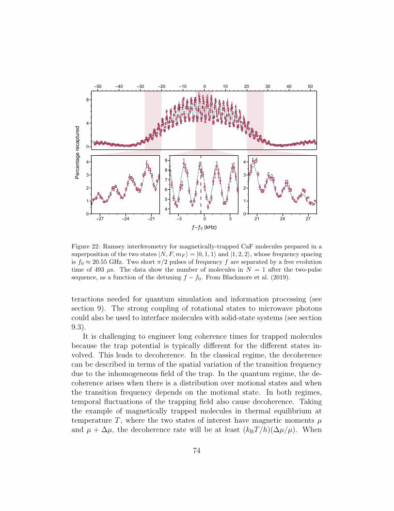
0

4

8

-50 -40 -30 -20 -10 0 10 20 30 40 50

0

1

2

3

4

-27 -24 -21

4

5

6

7

8

9

-3 0 30

1

2

3

4

21 24 27

Percentagerecaptured

ƒ-ƒ0 (kHz)

Figure 22: Ramsey interferometry for magnetically-trapped CaF molecules prepared in asuperposition of the two states |N,F,mF 〉 = |0, 1, 1〉 and |1, 2, 2〉, whose frequency spacingis f0 ≈ 20.55 GHz. Two short π/2 pulses of frequency f are separated by a free evolutiontime of 493 µs. The data show the number of molecules in N = 1 after the two-pulsesequence, as a function of the detuning f − f0. From Blackmore et al. (2019).

teractions needed for quantum simulation and information processing (seesection 9). The strong coupling of rotational states to microwave photonscould also be used to interface molecules with solid-state systems (see section9.3).

It is challenging to engineer long coherence times for trapped moleculesbecause the trap potential is typically different for the different states in-volved. This leads to decoherence. In the classical regime, the decoherencecan be described in terms of the spatial variation of the transition frequencydue to the inhomogeneous field of the trap. In the quantum regime, the de-coherence arises when there is a distribution over motional states and whenthe transition frequency depends on the motional state. In both regimes,temporal fluctuations of the trapping field also cause decoherence. Takingthe example of magnetically trapped molecules in thermal equilibrium attemperature T , where the two states of interest have magnetic moments µand µ + ∆µ, the decoherence rate will be at least (kBT/h)(∆µ/µ). When

74

T = 10 µK and (∆µ/µ) = 10−2, this rate is about 2 kHz.The coherent control of magnetically-trapped molecules has been studied

in Williams et al. (2018); Blackmore et al. (2019); Caldwell et al. (2020). Fig-ure 22 shows an example of Ramsey interferometry with CaF molecules in amagnetic quadrupole trap. Here, the molecules are prepared in a superposi-tion of two different rotational states, |N,F,mF 〉 = |0, 1, 1〉 and |1, 2, 2〉. For2Σ states, the Zeeman shifts of the stretched states6 are almost independentof the rotational quantum number N . This can be seen in figure 20 - noticethe nearly identical shifts of the uppermost level of each N . Consequently,transitions between these stretched states are relatively insensitive to mag-netic fields. The residual sensitivity is determined by the middle two termsin equation (70), whose coefficients are gl and gr. For many laser-coolablemolecules, there exist rotational transitions between stretched states wherethese two terms almost cancel, resulting in transitions that are exceptionallyinsensitive to magnetic fields (Caldwell et al., 2020). In these cases, longrotational coherence times are feasible for magnetically-trapped molecules.For CaF, the pair of states |0, 1, 1〉 and |1, 2, 2〉 have ∆µ/µ = −7.4 × 10−5,while the pair |1, 2, 2〉 and |2, 3, 3〉 have ∆µ/µ = −3.4 × 10−6. For the lat-ter pair, the magnetic sensitivity is so small that rotational coherence timesexceeding 1 s seem feasible for molecules cooled to 5 µK or below. So far,a coherence time of 6.4(8) ms has been demonstrated, limited by the largesize of the trapped cloud, an inhomogeneous change in phase resulting fromthe change in position of the molecules between microwave pulses, and ageometric phase which depends on the trajectory of each molecule betweenmicrowave pulses. These effects can be reduced by using smaller clouds anda magnetic trap geometry with a large bias field.

8. Optical traps

Optical dipole traps (Grimm et al., 2000) are commonly used to trap ul-tracold atoms and have recently been used to trap laser-cooled molecules (An-deregg et al., 2018; Cheuk et al., 2018). They have smaller volumes and lowerdepths than magnetic traps, but they can be used to trap molecules in anyinternal state and they can provide much tighter confinement. Importantly,the molecules can be cooled inside the trap, which can significantly enhance

6The stretched states are the ones with maximal (or minimal) values of all projectionquantum numbers, here mN , mS and mI .

75

both the spatial and phase-space densities. There are many possible con-figurations of optical dipole traps, but the most common uses light that isred detuned from all electronic transitions. The interaction of the inducedelectric dipole moment with the electric field of the light – the ac Starkshift – produces a potential proportional to the intensity, which attracts themolecule to the location of highest intensity. Here, we first outline the theoryof the ac Stark effect and then describe recent work on optical trapping oflaser-cooled molecules.

8.1. AC Stark effect

The theory of the ac Stark effect for a diatomic molecule is given in theappendix of Caldwell and Tarbutt (2020c). Here we highlight some salientfeatures. We consider a molecule interacting with light which has electricfield amplitude E0, angular frequency ωL, and unit polarization vector ε:~E = 1

2E0(εe−iωLt + ε∗eiωLt). It is convenient to write an effective operator for

the Stark effect that acts within a small subspace, often a single rotationalstate. This operator can be written in the form

HS =2∑

K=0

H(K)S = −E

20

4

2∑K=0

K∑P=−K

(−1)PA(K)P P

(K)−P . (73)

It is a sum of three parts, each of which is the scalar product of two rank-Kspherical tensors, a polarizability tensorA(K) that depends only on propertiesof the molecule, and a polarization tensor P(K) that depends only on thepolarization of the light. The matrix elements of H

(K)S can be expressed as

〈γ′|H(K)S |γ〉 = −E

20

4α(K)

K∑P=−K

(−1)Ph(γ, γ′, K, P )P(K)−P , (74)

where γ and γ′ stand for the set of quantum numbers needed to define stateswithin the subspace. The parameters α(K) depend on the frequency of thelight and the frequencies of transitions to states outside the subspace, whilethe factor h contains all of the dependence on the quantum numbers. Thescalar part produces the same shift for all states within the subspace, 〈H(0)

S 〉 =−α(0)E2

0/4, where α(0) is the scalar polarizability. The vector (α(1)) andtensor (α(2)) polarizabilities produce different shifts for different states. Thevector part is zero for a dc electric field. For an ac field it is only non-zerowhen the molecule has a spin and the light has a component of circular

76

Σ

Π

Σ

δfs

ωΣωΠ

ωL

(a)(b)

0.5 1.0 1.5 2.0-10

-5

0

5

10

ωL / ωΠ

α(K

) /(d2/ℏ

ωΠ)

(c)

0.96 0.98 1.00 1.02 1.04-200

-100

0

100

200

ωL / ωΠ

α(K

) /(d2/ℏ

ωΠ)

Figure 23: Polarizability for a model molecule. (a) Illustration of the model. (b) Polar-izability components versus laser frequency in scaled units. We have chosen ωΣ = 1.5ωΠ,δfs = ωΠ/50 and dΣ = dΠ = d. (c) Same as (b), plotted over a narrow range around theΣ−Π transition. Solid red: α(0). Dashed green: α(1). Dotted blue: α(2).

polarization. The effect of the vector part is the same as that of a magneticfield applied along the axis of circular handedness. Expressions for α(K) andh for molecules in 1Σ or 2Σ states are given in Caldwell and Tarbutt (2020c).

To illustrate the dependence of the polarizability components on the fre-quency of the light, ωL, we consider a model molecule with an electronicenergy structure as depicted in figure 23(a). This structure is typical formany molecules with 1Σ or 2Σ ground states. The model has two electronicexcited states, a Π state and a Σ state, with energies ~ωΠ and ~ωΣ above theground state. Due to the spin-orbit interaction, the Π state is split into twofine-structure components shifted by ±δfs/2 (with δfs = 0 for a 1Π state). Thetransition dipole moments for transitions from the ground state to the Π andΣ states are dΠ and dΣ. For convenience, we introduce the scaled quantitiesl = ωL/ωΠ, s = ωΣ/ωΠ, and f = δfs/ωΠ. In this model, the polarizabilitycomponents are

α(0) =1

3

(α|| + α⊥,− + α⊥,+

), (75a)

α(1) =1

2(β⊥,− − β⊥,+) , (75b)

α(2) =1

3

(2α|| − α⊥,− − α⊥,+

), (75c)

77

where

α|| =d2

Σ

~ωΠ

(1

s+ l+

1

s− l

), (76a)

α⊥,± =d2

Π

~ωΠ

(1

1± f/2 + l+

1

1± f/2− l

), (76b)

β⊥,± =d2

Π

~ωΠ

(1

1± f/2 + l− 1

1± f/2− l

). (76c)

Note that these results are relevant for frequencies far above rotational tran-sition frequencies. At microwave frequencies the polarizability is dominatedby the rotational structure, which is absent in our model.

Figure 23(b) plots these polarizability components for the case wheres = 3/2, f = 1/50 and dΣ = dΠ = d. The scalar polarizability, α(0), ispositive when the light is red detuned from all resonances (ωL < ωΠ), andnegative when blue detuned (ωL > ωΣ). It tends towards a constant in thelow frequency limit (ωL ωΠ) and towards zero in the high frequency limit(ωL ωΣ). It has a large magnitude near the resonances and changes signthrough them. The vector polarizability, α(1), is very small for all frequenciesother than ωL = ωΠ. Its behaviour in this region is best seen in the expandedview shown in figure 23(c). Halfway between the fine-structure components,α(1) is large whereas α(0) and α(2) both pass through zero. Away from reso-nances, |α(2)| is smaller than |α(0)| but much larger than |α(1)|. It thereforedominates the state-dependence of the polarizability in these regions. Thereis a range of frequencies between the Σ − Π and Σ − Σ transition frequen-cies where the polarizability is dominated by α(2) because α(0), α(1) are nearzero whereas α(2) is not. The behaviours of the polarizability componentsbetween resonances can be exploited to make state-dependent tweezer trapsas proposed by Caldwell and Tarbutt (2020a,b).

8.2. Optical dipole traps

When the ac Stark shift is either much smaller or much larger than otherrelevant interactions (e.g. hyperfine and Zeeman), the effect ofHS can be con-sidered in isolation leading to a shift of the form U = −αE2

0/4 = −αI/(2cε0),where I is the intensity of the light field and U is the potential in which themolecules move. Here, unlike above, we have not separated the polarizabilityinto its components. Instead, α is a parameter that depends on the state ofthe molecule and the polarization of the light. Its value can be determined

78

from the theory outlined above. In the case where the light is detuned farbelow all electronic resonances, α can be approximated by α(0), which in turncan be roughly estimated using equations (75) and (76).

A simple optical dipole trap is formed using a single, red detuned, focussedlaser beam. For a Gaussian beam with waist w0 and wavelength λ, theintensity distribution as a function of the radial and axial coordinates r andz is

I(r, z) =I0

1 + z2/z20

e−2r2/w2

, (77)

where w = w0

√1 + z2/z2

0 and z0 = πw20/λ. The intensity at the centre of

the focus is related to the power P by I0 = 2P/(πw20). For a molecule close

to the centre of the trap, we can expand equation (77) around r = z = 0,giving a trap potential

U(r, z) = −U0 +1

2mω2

r +1

2mω2

z , (78)

where ωr =√

4U0/(mw20) and ωz =

√2U0/(mz2

0) are the angular oscillationfrequencies in the radial and axial directions, and U0 = αI0/(2cε0) is the trapdepth.

Let us consider a CaF molecule in the state |N,F,mF 〉 = |1, 2,mF 〉interacting with light linearly polarized along the z-axis. For this case,α = α(0) + 1

10(2 − m2

F )α(2). Using the transition frequencies and dipolemoments for the A2Π − X2Σ+ and B2Σ+ − X2Σ+ transitions, and takinga wavelength of λ = 1064 nm, equations (75) and (76) give α(0), α(2) =2.97,−1.47 × 10−39 J (V m−1)−2. Taking P = 15 W, w0 = 45 µm andmF = 2, we find U0/kB = 210 µK, ωr = 2π × 1.2 kHz and ωz = 2π × 6.5 Hz.We should remember that all these values are approximate, since the realmolecule has more excited states than the model molecule. Nevertheless,they give reasonable estimates of the trap depths and oscillation frequenciesobtained for some typical parameters.

Laser cooled molecules were first trapped optically by Anderegg et al.(2018) who captured CaF molecules in a MOT, cooled them in an opticalmolasses, and then loaded them into a single-beam far-detuned optical dipoletrap with parameters similar to those considered above. They demonstratedthat sub-Doppler cooling works in the presence of the dipole trap, and thatcooling molecules into the trap increases the number captured by about afactor of five relative to direct capture. Approximately 150 molecules were

79

Figure 24: CaF molecules in an array of optical tweezer traps. (A) Images of the array.Upper image is averaged over 500 shots, and lower image is a single shot showing threeoccupied tweezer traps. Colour scale indicates signal per pixel. (B) Probability versusnumber of tweezer traps loaded. From Anderegg et al. (2019). Reprinted with permissionfrom AAAS.

trapped at a temperature of 60 µK and a density of 8(2)×107 cm−3. The traplifetime was found to be 750(40) ms, limited by collisions with backgroundgas. The group went on to show that Λ-enhanced cooling (see section 6) alsoworks in the presence of the dipole trap, and that it improves the loadingefficiency and final temperature (Cheuk et al., 2018). They were able toload 1300(60) molecules at a temperature of 21(3) µK and a peak densityof 6(2) × 108 cm−3, corresponding to a peak phase-space density of about7 × 10−8. They also showed that, in this configuration, the molecules canscatter more than 104 photons from the molasses before being lost from thetrap, providing an efficient method for imaging single trapped molecules.

8.3. Optical tweezer traps

A tweezer trap is an optical dipole trap that is very tightly focussed sothat the beam waist is about the same size as the wavelength of the light.In such a tightly confining trap, and in the presence of near-resonant cool-ing light, rapid light-assisted collisions ensure that only a single particle canbe trapped (Schlosser et al., 2001). This is sometimes known as collisionalblockade. An array of tweezer traps with adjustable spacing can be ob-tained by passing the beam through a spatial light modulator or an acousto-optical deflector driven by multiple rf frequencies (Bergamini et al., 2004;Gauthier et al., 2021). Great strides have been made with atoms in tweezertraps, including the near-deterministic loading of single atoms by tailoring

80

the light-assisted collisions (Grunzweig et al., 2010; Brown et al., 2019), Ra-man sideband cooling to the motional ground state (Kaufman et al., 2012;Thompson et al., 2013), re-arrangement of tweezer arrays to produce desiredconfigurations (Endres et al., 2016; Barredo et al., 2016), tweezer array opti-cal clocks (Norcia et al., 2019), and the association of atoms into moleculesinside tweezer traps (Liu et al., 2019; Zhang et al., 2020).

Recently, an optical tweezer array of laser cooled molecules was formed byAnderegg et al. (2019). A 780 nm beam was focussed to a spot size of 2.3 µm,and a one-dimensional array of these traps was created using an acousto-optic deflector. Single CaF molecules from the optical dipole trap discussedabove were loaded into these tweezer traps in the presence of the Λ-enhancedmolasses, and were detected with 92% fidelity by imaging their fluorescenceonto a camera. Figure 24 shows both single shot and averaged images of thetweezer array, along with a plot showing the probability distribution of thenumber of traps loaded. The average loading probability per trap is 34%.The radial oscillation frequency in the trap was measured to be 35 kHz, andthe temperature was 80(20) µK. When there are two molecules in the sametrap, the peak density is 3× 1010 cm−3 and the peak phase-space density is3×10−7. The authors demonstrated that, in the presence of the cooling light,light-assisted collisions occur on a timescale of a few milliseconds, resultingin a collisional blockade that ensures an occupancy of zero or one.

Using their tweezer trap array, Cheuk et al. (2020) measured inelastic col-lisions between pairs of CaF molecules prepared in selected quantum states.They used a pair of traps, measured the initial occupancies of the pair byfluorescence imaging, prepared the trapped molecules in a selected sub-levelof the rotational ground state using optical pumping and microwave transfer(see section 7.2), merged the pair into a single trap so that collisions couldoccur, then separated the traps again and re-measured their occupancies.They measured rapid two-body loss with no dependence on the choice of hy-perfine or Zeeman state, and attributed this loss either to the energeticallyallowed chemical reaction CaF + CaF → CaF2 + Ca, or to the formation ofcomplexes that are undetected or lost by photoexcitation. This ability tomeasure collisional processes between molecules at the single particle level isa valuable new tool for physics and physical chemistry.

An important current challenge is to obtain full quantum control overthe molecules by cooling them to the motional ground state of the tweezertrap. For atoms, Raman sideband cooling is commonly used (Kaufman et al.,2012; Thompson et al., 2013). This is done by repeatedly applying a two-

81

-1.0 -0.5 0.0 0.5 1.0-1.0

-0.5

0.0

0.5

1.0

x (μm)

z(μm)

(a)

0

0.2

0.4

0.6

0.8

1.0

-1.0 -0.5 0.0 0.5 1.0-1.0

-0.5

0.0

0.5

1.0

x (μm)

z(μm)

(b)

-0.2

-0.1

0

0.1

0.2

Figure 25: Contour plots in the plane of the focus of an optical tweezer trap, for 780 nmlight propagating along y and focussed by a 0.55 NA lens. The input beam is polarizedalong x and has a 1/e2 diameter equal to the lens diameter. (a) Intensity distributionI(x, z)/Imax. (b) Scaled component of ellipticity in the z direction, (I(x, z)/Imax)Cz(x, z).

step process where the first step drives a Raman transition between twointernal states and reduces the motional quantum number, and the secondstep optically pumps back to the original internal state. The first step iscoherent and needs to be slow enough to resolve the motional states, whilethe second step provides dissipation. The application of Raman sidebandcooling to molecules in tweezer traps is discussed in Caldwell and Tarbutt(2020c). Strong tensor Stark shifts result in different trap potentials forthe two internal states involved in the cooling, resulting in two significantproblems: (i) the Raman transition frequency depends on the motional stateand (ii) there is an additional contribution to the heating in the opticalpumping step as the molecule is suddenly transferred into a different trap.These problems can be solved by applying a magnetic field that is strongenough to uncouple the rotational angular momentum from the spin, so thatlevels are well characterized by mN , and then choosing a tweezer polarizationwhere the tensor Stark shift is identical for two different mN levels. Toimplement sideband cooling in practice, it is beneficial to make the traps astightly-confining as possible, so that ωr and ωz are as large as possible. Thislowers the mean motional quantum number for a given starting temperature,and makes it easier to resolve the motional states.

Figure 25 shows some of the properties of an optical tweezer trap in theplane of the focus. Here, we have assumed that a Gaussian laser beam with

82

a wavelength of 780 nm is focussed by a lens with a numerical aperture (NA)of 0.55. The input beam propagates along y, is polarized along x and hasa 1/e2 diameter equal to the lens diameter. We use the vector Debye inte-gral (Richards and Wolf, 1959) to calculate the electric field components inthe region of the trap. Figure 25(a) shows the intensity distribution at thefocus, I(x, z)/Imax where Imax is the maximum intensity. The distribution isGaussian in both directions but is slightly elliptical, having a 1/e2 radius of0.69 µm along z and 0.74 µm along x. This leads to different trap frequen-cies in these two directions. Near the focus, the electric field has componentsalong x and y, resulting in spatially-varying elliptical polarization about thez-axis (Richards and Wolf, 1959). We characterize this using the quantity~C = Im(ε × ε∗), where ε is a unit polarization vector. The magnitude of~C gives the degree of ellipticity, with C = 1 corresponding to circular po-larization and C = 0 to linear polarization, and the direction gives the axisof ellipticity. Figure 25(b) shows (I(x, z)/Imax)Cz(x, z) in the plane of thefocus. We find significant circular polarization components with oppositehandedness on either side of the focus. For a molecule with spin, the inter-action with the light field depends on the handedness and on the directionof the spin, resulting in a contribution to the ac Stark shift that is propor-tional to α(1)mFCzI, where mF is the projection of the angular momentumonto z. In the context of equation (73), ~C = P(1), the rank-1 component ofthe spherical tensor formed from ε and ε∗, and its interaction with the rank-1 component of the polarizability tensor A(1) results in a vector Stark shift.Caldwell and Tarbutt (2020a) have shown how this interaction can be used tocreate state-dependent optical tweezer traps that can trap pairs of moleculesat separations much smaller than otherwise possible. As can be seen fromfigure 23(c), α(1) dominates the polarizability when the frequency of the lightlies between the two fine-structure components of the excited state. In thiscase, molecules with opposite mF are trapped on opposite sides of the focus(at the location of the maximum and minimum in figure 25(b)). Introduc-ing an additional tweezer at a wavelength where α(0) dominates squeezes thetwo molecules together. This can be used to enhance dipolar interactionsbetween molecules, which is important for quantum simulation and informa-tion processing. A similar outcome can also be achieved by exploiting thetensor polarizability, as described in Caldwell and Tarbutt (2020b).

83

9. Applications and future directions

Ultracold molecules can be used to search for new physics, explore thephysics of many-body quantum systems, store and process quantum infor-mation, and probe the quantum mechanical underpinnings of chemistry andcollisions. In this section, we briefly explore some of these exciting applica-tions. We note that the ultracold molecules needed can also be producedby other methods, including atom association (Ni et al., 2008), optoelectricSisyphus cooling (Prehn et al., 2016), and electrodynamic slowing and fo-cussing (Cheng et al., 2016). Here, we will highlight the particular role thatlaser cooled molecules can play.

9.1. Controlling dipole-dipole interactions

Many of the applications of ultracold molecules hinge on dipole-dipoleinteractions between two or more molecules. For two molecules i and j, withposition vectors ~ri and ~rj, the dipole-dipole interaction Hamiltonian is

Hdd =1

4πε0

~di · ~dj − 3(~di · eij)(~dj · eij)r3ij

. (79)

Here, ~di and ~dj are the dipole moment operators for the two molecules, ~rij =~ri−~rj is their relative displacement, and eij = ~rij/rij is a unit vector pointingalong ~rij. This form of the interaction is especially useful for molecules whichare fixed in place, e.g. molecules in an optical lattice or in tweezer traps. Inspherical tensor form, the interaction is

Hdd = −√

6

4πε0r3ij

2∑q=−2

(−1)qC2−q(θij, φij)T

2q (~di, ~dj). (80)

In this form, the relative displacement is expressed in spherical polar coor-dinates (rij, θij, φij), C

2 is the re-normalized spherical harmonic of rank 2

(C2q =

√4π/5Y2,q), and T 2(~di, ~dj) is the rank-2 spherical tensor formed from

~di and ~dj. This form is most useful for freely moving molecules, and alsohelps to reveal the processes allowed via this interaction.

Let us consider the simple case of a two-level molecule with states |0〉 and|1〉 whose energies are 0 and E01. The states are chosen so that the transition

dipole moment ~d01 = 〈0|~d|1〉 is non-zero. In the two-molecule basis |00〉, |01〉,|10〉, |11〉, the only non-zero matrix elements of Hdd are the ones where both

84

(a)

0

1

02

1

302

1

0

0 5 10 15 20 25 30

-20

-10

0

10

Electric field (B/μe)

Energy(B)

(b)

0 5 10 15 20 25 30

-0.2

0.0

0.2

0.4

0.6

0.8

Electric field (B/μe)

Dipolemoment(μe)

Figure 26: (a) Energy levels of a rigid rotor molecule as a function of applied electric field.The levels are labelled by |mN |. (b) Corresponding dipole moments.

molecules change state. The coupling between |00〉 and |11〉 is usually verystrongly suppressed because the dipole-dipole interaction is tiny comparedto 2E01. Neglecting this, we are left only with the coupling between |01〉 and|10〉. The eigenstates are |00〉, |11〉, and |Ψ±〉 = 1√

2(|01〉± |10〉) with energies

0, 2E01 and E01 ± Edd where

Edd =1

4πε0r3ij

〈01|~di · ~dj − 3(~di · eij)(~dj · eij)|10〉. (81)

In the special case where |0〉 and |1〉 have the same value of mF , equation(81) simplifies to

Edd =|~d01.z|2

4πε0r3ij

(1− 3 cos2 θij), (82)

where θij is the angle between eij and the z-axis. We see that a pair ofmolecules prepared in |01〉 will oscillate back and forth between |01〉 and|10〉 at a characteristic frequency 2Edd/h. The single excitation is exchangedbetween the two molecules, mediated by the dipole-dipole interaction. Aswe will see, this exchange interaction can be used to implement a two-qubitgate and to explore aspects of quantum magnetism.

The exchange interaction does not require any applied electric field. Addingan electric field polarizes the molecules, introducing a direct dipole-dipole

85

interaction between them. Taking |0〉 and |1〉 to be the eigenstates in thepresence of the electric field, Hdd now has diagonal matrix elements as wellas the off-diagonal ones described above. To determine the induced dipolemoments we first calculate the dc Stark shift of the molecule. For a moleculein a Σ state, the Stark shift is dominated by mixing of rotational states andall other structure of the molecule can often be neglected. This is sometimesdescribed as the Stark shift of a rigid rotor. In this simple case, the relevantHamiltonian is

HRR−Stark = B ~N2 − µeE cos Θ, (83)

where B is the rotational constant, ~N is the rotational angular momentum,µe is the molecule-frame dipole moment, E is the applied electric field, andΘ is the angle between the internuclear axis and the electric field direction.Figure 26(a) shows the eigenvalues of HRR−Stark as function of E . The energy,WStark, is expressed in units of B, and the electric field in units of (B/µe),making this a universal plot. The states |N,mN〉 and |N,−mN〉 remain de-generate in the electric field, so each rotational manifold splits into N + 1components labelled by |mN |. Figure 26(b) shows the induced dipole mo-ments of the various states, 〈d〉 = −dWStark/dE , as a function of E . Here,the dipole moments are in units of µe. At low fields, some of the dipolesare positive and some negative, while at high fields they tend towards µe asthe molecule becomes fully polarized along the field direction. When onemolecule is in state |a〉 and the other in state |b〉 (a, b ∈ 0, 1), the diagonalelements of Hdd are

〈ab|Hdd|ab〉 =〈a|d|a〉〈b|d|b〉

4πε0r3ij

(1− 3 cos2 θij), (84)

where the dipole moments 〈a|d|a〉, 〈b|d|b〉 can be read from figure 26(b).Instead of using a static electric field, the dipole moments can also be

induced using an oscillating field near resonant with the transition from |0〉to |1〉. For molecules, this is most likely to be a microwave field close toresonance with a rotational transition. In the interaction picture, the neweigenstates are

|±〉 = N

(−∆±

√∆2 + Ω2

Ω|0〉+ |1〉

)(85)

with eigenvalues ±~2

√∆2 + Ω2. Here, Ω is the Rabi frequency, ∆ is the

detuning from resonance, and N is the normalization factor. These states

86

have dipole moments and the pair of molecules will interact through thedipole-dipole interaction. For example, if we take a microwave field polarizedin the z direction, and prepare both molecules in |+〉, or both in |−〉, Hdd

has the diagonal elements

〈± ± |Hdd| ± ±〉 =|~d01.z|2

4πε0r3ij

Ω2

Ω2 + ∆2(1− 3 cos2 θij). (86)

We see that the interaction can be controlled using the parameters of themicrowave field. A more detailed discussion of how microwave fields can beused to control the dipole-dipole interaction between molecules, and how thiscontrol can be used to build quantum gates, is given in Hughes et al. (2020).

9.2. Quantum simulation

Understanding many-body quantum systems, and engineering new ones,is an important research area with applications in condensed matter physics,nuclear and particle physics, cosmology, chemistry and biology. These sys-tems often exhibit remarkable phenomena, e.g. high temperature supercon-ductivity, but they are difficult to understand because the systems found innature are often difficult to control and impossible to simulate with a clas-sical computer once more than a few interacting particles are involved. Ourunderstanding can be improved by engineering a well-controlled quantumsystem so that it emulates a many-body problem of interest. We derive amodel Hamiltonian that captures the main features of the real system, andthen build a physical system that implements this model. This is knownas quantum simulation (Feynman, 1982; Deutsch, 1985). Arrays of ultra-cold atoms and molecules are well suited to this task. Their benefits includecontrol of the particle positions and interaction strengths, the number ofaccessible dimensions, whether real or synthetic (Sundar et al., 2018), trapdepths, and often the ability to address single particles.

To date, much of the work in this field has used ultracold atoms trappedin optical lattices to investigate corresponding systems in condensed matterphysics. This has led, for example, to significant insight into the quantumphase transition between a superfluid and a Mott insulator (Greiner et al.,2002), and models of antiferromagnetism (Mazurenko et al., 2017). Atomsinteract through the van der Waals interaction, which is short range, orthrough magnetic dipole-dipole interactions, which are long range but usu-ally quite weak. This limits the scope of accessible problems. By contrast,

87

Jz

J⟂

V

W

0 10 20 30 40 50

-2

0

2

4

6

Electric field (kV/cm)

Interactionstrength

(kHz)

Figure 27: Strength of parameters appearing in the many-body Hamiltonian, equation(87), as a function of electric field, for CaF molecules in a 1064 nm lattice.

molecules interact through long-range electric dipole-dipole interactions thatcan be tuned using static or microwave electric fields, as discussed in section9.1.

To glimpse the richness of arrays of interacting molecules, let us considerthe simple case where we apply a dc electric field along z, neglect hyperfineand spin-rotation interactions, and focus only on the states | ↑〉 and | ↓〉 thatcorrelate to the field-free states |N,mN〉 = |0, 0〉 and |1, 0〉. We can re-writeHdd from equation (79) in terms of the spin-1/2 operators acting on moleculei, Szi , S±i , and then sum over all pairs of molecules in the lattice, to arrive atthe many-body Hamiltonian (Gorshkov et al., 2011; Hazzard et al., 2014)

H =1

2

∑i 6=j

Vdd

[JzS

zi S

zj +

J⊥2

(S+i S−j + S−i S

+j ) +W (Szi nj + niS

zj ) + V ninj

].

(87)Here, ni is the number operator at site i, Vdd = (1 − 3 cos2 θij)/r

3ij, and we

have re-expressed the positions of the molecules (ri, rj) in terms of the latticeconstant a. The first term in equation (87), with parameter Jz, describes anIsing-type spin-spin interaction, the second term (parameter J⊥) describesthe exchange of excitations, the third (parameter W ) is a spin-density inter-action where a molecule at one site creates an effective magnetic field alongz for a spin on another site, and the fourth term (parameter V ) describesdensity-density interactions. We see that a lattice of polar molecules is anextremely rich system, even in this very simple case. The Hamiltonian is

88

long range in 3D, and is anisotropic in both space and spin. In the case ofunit filling, the V term is a constant and the W term is similar to a uniformmagnetic field, and both can be neglected. The resulting Hamiltonian is theXXZ model. This reduces to the Ising model when J⊥ = 0, to the XX modelwhen Jz = 0, and to the Heisenberg model when J⊥ = Jz.

The parameters of the model are related to molecular properties as

Jz =(d↑ − d↓)2

4πε0a3, (88a)

J⊥ =2d2↑↓

4πε0a3, (88b)

W =(d2↑ − d2

↓)

8πε0a3, (88c)

V =d↑ + d↓16πε0a3

, (88d)

where d↑ = 〈↑ |dz| ↑〉, d↓ = 〈↓ |dz| ↓〉 and d↑↓ = 〈↑ |dz| ↓〉. Figure 27shows how the parameters depend on electric field for CaF molecules in a1064 nm lattice. The parameters can be significantly larger than single-particle decoherence rates, and their relative strengths are highly tunable,allowing the many-body physics to be explored across a large parameterspace.

Dipole-mediated spin exchange interactions have already been studied ina lattice of ultracold KRb molecules formed by atom association (Yan et al.,2013), and the application of electric fields will allow other aspects of themodel to be explored using this system. Other exotic quantum phases arealso within experimental reach (Buchler et al., 2007; Cooper and Shlyap-nikov, 2009; Yao et al., 2013). As the phase-space density of laser-cooledmolecules is increased towards quantum degeneracy (see section 9.4), theywill be able to contribute to this field. They have much to offer, since theycan be detected efficiently, state-selectively, and non-destructively by laser-induced fluorescence imaging, and often have large electric dipole moments.They also often have both electron and nuclear spin degrees of freedom,which provide even more richness and control and can be used to engineeralmost any lattice spin model of interest (Micheli et al., 2006). With the ad-dition of tunnelling between sites, the system models an extended HubbardHamiltonian with long-range interactions (Wall and Carr, 2010; Wall et al.,2013). The ability to explore these models with such control can help solve

89

long-standing problems in many-body quantum physics.

9.3. Quantum information processing

Currently, quantum information processing with molecules is nowherenear as advanced as for atoms and ions (Cirac and Zoller, 1995; Wang et al.,2016; Ballance et al., 2016). However, molecules offer many intriguing advan-tages, including long coherence times (Park et al., 2017), very fast single qubitmanipulation using microwave fields, fast two-qubit gates using dipole-dipoleinteractions, and the potential for electric dipole coupling of the molecules tophotonic or solid-state systems. There are many ideas of how to make use ofthese advantages (DeMille, 2002; Yelin et al., 2006; Andre et al., 2006; Karraet al., 2016; Ni et al., 2018; Yu et al., 2019; Albert et al., 2020; Sawant et al.,2020; Hughes et al., 2020). We consider here two interesting approaches.

The first approach is to use molecules in arrays of tweezer traps. Thisis attractive because the arrays can be rearranged, pairs can be broughttogether to implement two-qubit gates, and single-site addressability andreadout can be engineered using electric or magnetic field gradients, or byadjusting the laser intensity at a selected site to change the local ac Starkshift. As discussed in section 8.3, tweezer arrays of molecules have alreadybeen formed (Anderegg et al., 2019) and rearrangement protocols can fol-low those already established for atoms (Barredo et al., 2016). Importantnext steps are to: (i) increase the trap frequencies by making smaller traps;(ii) cool the molecules to the motional ground state (Caldwell and Tarbutt,2020c); (iii) control tensor Stark shifts in order to engineer long rotationalcoherence times in the trap (Seeßelberg et al., 2018); (iv) implement state-dependent traps that can bring pairs of molecules very close together inorder to enhance the dipole-dipole interactions between them (Caldwell andTarbutt, 2020a,b).

A second interesting approach, expounded by Andre et al. (2006), is totrap molecules close to the surface of a chip where they can be coupled tosuperconducting microwave resonators fabricated on the same chip, forminga monolithic hybrid quantum processor. The molecules can be trapped usingmicrofabricated electric or magnetic surface traps. The microwave resonator,tuned into resonance with a rotational qubit in the molecule, facilitates trans-fer of quantum information between the molecule and a microwave photonand can be used to couple selected distant molecules together. Many of theelements needed to realize these ideas are established or emerging. The fab-rication techniques needed to make microscopic traps are the same as those

90

used to make atom chips, which are becoming a mature technology. Mag-netic trapping of laser-cooled molecules is established, though increases inphase-space density will be needed to load molecules efficiently into micro-scopic traps. Superconducting resonators with high quality factors have beenfabricated on chips and have been coupled to ground-state atoms through themagnetic dipole interaction (Hattermann et al., 2017) and to Rydberg atomsthrough the electric dipole interaction (Morgan and Hogan, 2020).

9.4. Ultracold collisions, collisional cooling, and chemistry

Another research area where laser-cooled molecules are useful, and wherethey may enable entirely new areas of study, is the investigation of interac-tions of molecules at close range, i.e. collisions and chemical reactions (Hea-zlewood and Softley, 2021). The control of these interactions through choiceof quantum state, molecular orientation, and applied field have been inves-tigated by many authors (Krems, 2005, 2008; Ospelkaus et al., 2010; Bohnet al., 2017; Hu et al., 2020).

A full understanding of the quantum chemistry of molecules often re-quires an in-depth investigation of their elastic (momentum changing), in-elastic (quantum state changing), and reactive (chemical species changing)collisions. Measurements of elastic and inelastic cross sections can be sen-sitive probes of the multi-dimensional potential energy surfaces, which areinherently difficult to calculate accurately. In the ultracold regime, experi-ment and theory come together in an exciting interplay that is revealing thequantum-mechanical underpinnings of particle interactions. At normal tem-peratures, molecules populate a large number of internal quantum states andinteractions can often energetically access a vast array of possible pathwaysbetween the reactant and product states. When cold, only a few quantumstates are populated and many reaction pathways become energetically in-accessible, proceeding instead via quantum tunneling, entanglement, or res-onances (Chandler, 2010; Richter et al., 2015; Toscano et al., 2020). In theultracold limit, interactions involve only one or a few partial waves. Forsimple systems consisting of, e.g., pairs of alkali-metal atoms or light atom-molecule systems, it is possible to solve the multi-dimensional Schrodingerequation numerically using coupled-channel methods. For heavier or morecomplex systems, or at higher temperature, the number of channels neededfor convergence quickly becomes computationally prohibitive. Remarkableprogress has been made in bi-alkali systems by instead formulating effective

91

single-channel models based on quantum defect theory (Idziaszek and Juli-enne, 2010; Gao, 2010; Kotochigova, 2010; Frye et al., 2015; He et al., 2020a).Amazingly, by incorporating only a couple of free parameters, such modelscan often predict dynamical rates and the positions and strengths of colli-sional resonances in the presence of external electromagnetic fields. Evenmore striking is the emergence of universal behaviours in these complex andapparently distinct systems (Idziaszek and Julienne, 2010; Julienne et al.,2011). Expanding these models to predict the behavior of new ultracoldspecies produced using laser cooling is a likely next step.

Collisional cooling will almost certainly be needed to increase the phase-space density of laser-cooled molecules towards quantum degeneracy. Oneoption is sympathetic cooling with ultracold atoms (Lim et al., 2015; Sonet al., 2020), and another is evaporative cooling of the molecules (Valtolinaet al., 2020). In both cases the ratio of elastic to inelastic collision ratesis critical - the elastic collisions are needed for thermalization, whereas in-elastic collisions typically lead to trap loss. To establish good collisionalcooling routes it is important to study these elastic and inelastic processesand learn to control them. There has been a great deal of theoretical workon sympathetic cooling of molecules (Soldan et al., 2002; Krems et al., 2003;Lara et al., 2006; Wallis et al., 2011; Gonzalez-Martınez and Hutson, 2011;Tscherbul et al., 2011), and recent experiments in this direction have begunto study collisions between laser-cooled molecules and atoms (Jurgilas et al.,2021). Evaporative cooling of molecules can be assisted by using an electricfield to introduce dipolar interactions that enhance elastic collision rates.Indeed, when the dipoles become large enough, the scattering enters a uni-versal regime and the elastic cross section can be exceptionally large (Bohnet al., 2009). Amazingly, inelastic and reactive collisions are very stronglysuppressed at electric fields where the energy of a pair of molecules preparedin one configuration (e.g. both in (N,mN) = (1, 0)) crosses that of a differentconfiguration (e.g. one in (0, 0) and the other in (2, 0)). As the moleculesapproach from any angle, the dipole-dipole interaction turns the crossinginto an avoided crossing, resulting in a large repulsive barrier at long range,which prevents the molecules getting close enough for inelastic or reactivecollisions. This electric shield has been studied theoretically (Avdeenkovet al., 2006; Quemener and Bohn, 2016) and recently demonstrated experi-mentally (Matsuda et al., 2020). Theoretical work also shows how to shieldagainst unwanted collisions using a microwave field (Karman and Hutson,2018). A remarkable recent experiment with CaF molecules in tweezer traps

92

has demonstrated such microwave shielding, showing a reduction in inelasticloss by a factor of six (Anderegg et al., 2021).

A striking example of experimental progress in ultracold chemistry, isthe controlled formation of a single molecule from two individual atoms (Liuet al., 2018; Zhang et al., 2020; He et al., 2020b). Another example is thecomplete mapping of a chemical reaction, including direct observations ofreactants, transient intermediate complexes, and products (Hu et al., 2019).A third is the study of collisions between laser-cooled molecules in opticaltweezers at the single particle level (Cheuk et al., 2020). Laser cooling di-versifies the set of species and properties available for studying chemistryat ultracold temperatures. Laser cooling of chemically important diatomicspecies, such as CH and NH, and more complex polyatomic species, will en-rich this topic. It may eventually be possible to fully understand and controlthe emergence of chemical complexity in cold, low density environments likethose found in the interstellar medium and planetary atmospheres (Smithand Rowe, 2000; Herbst and van Dishoeck, 2009).

9.5. Probing fundamental physics

Laser cooled molecules can be used to search for new particles and forcesbeyond the standard model of particle physics (DeMille et al., 2017; Safronovaet al., 2018). This can be done by making ultra-precise measurements thattest the discrete symmetries of nature – charge conjugation (C), parity (P),and time-reversal (T). Laser-cooled molecules can greatly increase the pre-cision of such measurements. A great example is the ongoing search forthe electric dipole moment (EDM) of the electron, which is associated withnew sources of charge-parity (CP) violation required to explain the observedmatter / anti-matter imbalance in the Universe. CP violation in the stan-dard model fails, by many orders of magnitude, to explain this imbalance.Many extensions of the standard model introduce new sources of CP vio-lation which naturally grant the electron an electric dipole moment largeenough to measure. Precise measurements using heavy dipolar moleculesare one of the best ways to verify, or eliminate, these theories experimen-tally (Hinds, 1997). Intriguingly, state-of-the-art experiments (Cairncrosset al., 2017; Andreev et al., 2018) now probe deep into the parameter spaceof many standard model extensions. Currently, the most sensitive experi-ments use molecules that combine the inherent sensitivity of a heavy atomtogether with the high polarizability of a polar molecule. All currently usemolecules at temperatures above 1 K. Laser cooling can hugely increase the

93

coherence time in these experiments, and can facilitate entirely new exper-imental techniques (Tarbutt et al., 2013; Aggarwal et al., 2018; Lim et al.,2018; Augenbraun et al., 2020c; Fitch et al., 2020; Hutzler, 2020). Such ex-periments are projected to increase experimental sensitivity to the EDM byone or two orders of magnitude over the coming decade.

A fascinating new avenue is the use of laser cooled polyatomic moleculesfor testing T-violating effects such as electric dipole or magnetic quadrupolemoments (Augenbraun et al., 2020c; Hutzler, 2020; Maison et al., 2019; De-nis et al., 2020). Molecules such as YbOH (Kozyryev and Hutzler, 2017)and HgOH (Mitra et al., 2021) have high sensitivity to T-violating effects,are laser coolable, and provide robust control of systematic errors. Dueto their closely spaced parity doublets (l-doubling, see section 2.9) thesemolecules can be fully polarized in a small electric field and provide inter-nal co-magnetometry. Experiments with these molecules may ultimately belimited only by the available coherence time, which for YbOH is ≈1 s dueto the relatively high energy and anharmonicity of the l-doublet used (Au-genbraun et al., 2020b). Even higher sensitivities may be accessible by usingsystems with lower energy parity doublets, such as isoelectronic nonlinearpolyatomic molecules like YbOCH3 (Augenbraun et al., 2020b). Here, paritydoublets arising from rigid-body rotation (K-doublets) are even more closelyspaced and have lower overall energies, leading to longer coherence times andfull polarization in even smaller electric fields. Another benefit is that thechemical substitution of H by CH3 is expected to improve the Franck-Condonfactors at the expense of only slightly increasing the mass, which may makelaser cooling easier. Measurements of electric dipole moments with thesesystems may ultimately probe new physics with equivalent energies at thePeV scale (Kozyryev et al., 2017).

Molecules are also being used to measure the nuclear anapole moment,a signature of P-violation due to interactions in nuclei involving the weakforce (Cahn et al., 2014; Altuntas et al., 2018). These experiments could alsobenefit from laser cooling. Also of interest is the parity-violating energy dif-ference between left- and right-handed chiral molecules, which was predictedlong ago but has never been measured (Quack et al., 2008; Tokunaga et al.,2013). Noting the recent progress with large molecules, it now seems feasibleto apply laser cooling to chiral species (Isaev and Berger, 2018; Augenbraunet al., 2020a).

Molecules can also be used to test the hypothesis that fundamental con-stants may depend on time, space, or the local density of matter. Such

94

variations are predicted by grand-unified theories and by some theories ofdark matter and dark energy (Olive and Pospelov, 2010; Uzan, 2011). Tran-sitions in molecules depend mainly on two fundamental constants, the fine-structure constant α and the proton-to-electron mass ratio mp/me. For ex-ample, rotational and vibrational transition frequencies scale as (mp/me)

−1

and (mp/me)−1/2, respectively. Furthermore, when the transition energy re-

sults from a near cancellation between two large contributions of differentorigin, certain transitions will exhibit even greater sensitivities (Chin et al.,2009). Laboratory experiments can be compared to astronomical observa-tions to probe variations on cosmological scales (Safronova et al., 2018), ashas been done using beams of OH (Hudson et al., 2006) and CH (Truppeet al., 2013). Ultra-precise laboratory measurements over a timescale of a fewyears test the present-day drift or oscillation of the constants. To date, themost stringent limits come from atomic clock measurements (Schwarz et al.,2020; Lange et al., 2021). Clocks based on transitions in ultracold moleculesare currently under development. For example, a direct limit on the time vari-ation of mp/me has been obtained using ultracold KRb molecules (Kobayashiet al., 2019), a fountain of ultracold NH3 molecules has been demonstrated,and a clock based on a vibrational transition in Sr2 molecules in an opticallattice is being developed (Kondov et al., 2019). Clocks based on vibra-tional transitions in laser-cooled molecules are an attractive complementaryapproach (Kajita, 2018).

10. Concluding remarks

The extension of laser cooling and trapping methods from atoms tomolecules has made huge progress over the last decade. The field continuesto expand rapidly and is moving from the development of techniques towardsmany exciting applications. We anticipate a great number of developmentsover the next few years. These are likely to include new methods to slowmolecules more efficiently, a variety of new species being cooled and trapped,increases in phase-space density by collisional cooling together with shieldingof unwanted collisions, sideband cooling to bring molecules to the ground-state of a trap, control of dipole-dipole interactions to entangle molecules,improvements to hyperfine and rotational coherence times in magnetic andoptical traps, small-scale quantum simulations, and the first tests of funda-mental physics using laser cooled molecules. The continued flourishing of thisfield will help to link molecular physics with numerous other sciences includ-

95

ing quantum science and technology, condensed matter physics, chemistry,metrology, high energy physics, and cosmology.

Acknowledgements

We thank Helene Perrin, Daniel McCarron, Stefan Truppe, and Ben Sauerfor their careful reading and helpful feedback on this manuscript. We ac-knowledge generous support from EPSRC (grant EP/P01058X/1), STFC(grant ST/S000011/1), the John Templeton Foundation (grant 61104), theGordon and Betty Moore Foundation (grant 8864), the Alfred P. Sloan Foun-dation (grant G-2019-12505), and the Royal Society.

References

Agarwal, G. S., Mølmer, K., 1993. Correlation-function approach to the mo-mentum diffusion of atoms moving in standing waves. Phys. Rev. A 47,5158.

Aggarwal, P., Bethlem, H. L., Borschevsky, A., Denis, M., Esajas, K., Haase,P. A. B., Hao, Y., Hoekstra, S., Jungmann, K., Meijknecht, T. B., Mooij,M. C., Timmermans, R. G. E., Ubachs, W., Willmann, L., Zapara, A.,2018. Measuring the electric dipole moment of the electron in BaF. Eur.Phys. J. D 72, 197.

Akerman, N., Karpov, M., Segev, Y., Bibelnik, N., Narevicius, J., Narevicius,E., 2017. Trapping of molecular oxygen together with lithium atoms. Phys.Rev. Lett. 119, 073204.

Albert, V. V., Covey, J. P., Preskill, J., 2020. Robust encoding of a qubit ina molecule. Phys. Rev. X 10, 031050.

Albrecht, R., Scharwaechter, M., Sixt, T., Hofer, L., Langen, T., 2020. Buffer-gas cooling, high-resolution spectroscopy, and optical cycling of bariummonofluoride molecules. Phys. Rev. A 101, 013413.

Altuntas, E., Ammon, J., Cahn, S. B., DeMille, D., 2018. Demonstrationof a sensitive method to measure nuclear-spin-dependent parity violation.Phys. Rev. Lett. 120, 142501.

96

Anderegg, L., Augenbraun, B. L., Bao, Y., Burchesky, S., Cheuk, L. W., Ket-terle, W., Doyle, J. M., 2018. Laser cooling of optically trapped molecules.Nat. Phys. 14, 890–893.

Anderegg, L., Augenbraun, B. L., Chae, E., Hemmerling, B., Hutzler, N. R.,Ravi, A., Collopy, A., Ye, J., Ketterle, W., Doyle, J. M., 2017. Radiofrequency magneto-optical trapping of CaF with high density. Phys. Rev.Lett. 119, 103201.

Anderegg, L., Burchesky, S., Bao, Y., Yu, S. S., Karman, T., Chae, E.,Ni, K.-K., Ketterle, W., Doyle, J. M., 2021. Observation of microwaveshielding of ultracold molecules. arXiv: 0902:0885.

Anderegg, L., Cheuk, L. W., Bao, Y., Burchesky, S., Ketterle, W., Ni, K.-K.,Doyle, J. M., 2019. An optical tweezer array of ultracold molecules. Science365, 1156–1158.

Andre, A., DeMille, D., Doyle, J. M., Lukin, M. D., Maxwell, S. E., Rabl,P., Schoelkopf, R. J., Zoller, P., 2006. A coherent all-electrical interfacebetween polar molecules and mesoscopic superconducting resonators. Nat.Phys. 2, 636–642.

Andreev, V., Ang, D. G., DeMille, D., Doyle, J. M., Gabrielse, G., Haefner,J., Hutzler, N. R., Lasner, Z., Meisenhelder, C., O’Leary, B. R., Panda,C. D., West, A. D., West, E. P., Wu, X., 2018. Improved limit on theelectric dipole moment of the electron. Nature 562, 355–360.

Atutov, S., Biancalana, V., Burchianti, A., Calabrese, R., Gozzini, S.,Guidi, V., Lenisa, P., Marinelli, C., Mariotti, E., Moi, L., Nasyrov, K.,Pod’yachev, S., 2001. Sodium MOT collection efficiency as a function ofthe trapping and repumping laser frequencies and intensities. Eur. Phys.J. D 13 (1), 71–82.

Augenbraun, B. L., Doyle, J. M., Zelevinsky, T., Kozyryev, I., 2020a. Molecu-lar asymmetry and optical cycling: laser cooling asymmetric top molecules.Phys. Rev. X 10, 031022.

Augenbraun, B. L., Lasner, Z. D., Frenett, A., Sawaoka, H., Le, A. T.,Doyle, J. M., Steimle, T. C., 2020b. Observation and laser spectroscopy ofytterbium monomethoxide, YbOCH3. arXiv: 2012.01212.

97

Augenbraun, B. L., Lasner, Z. D., Frenett, A., Sawaoka, H., Miller, C.,Steimle, T. C., Doyle, J. M., 2020c. Laser-cooled polyatomic moleculesfor improved electron electric dipole moment searches. New J. Phys. 22,022003.

Avdeenkov, A. V., Kajita, M., Bohn, J. L., 2006. Suppression of inelasticcollisions of polar 1Σ state molecules in an electrostatic field. Phys. Rev.A 73, 022707.

Ballance, C. J., Harty, T. P., Linke, N. M., Sepiol, M. A., Lucas, D. M., 2016.High-fidelity quantum logic gates using trapped-ion hyperfine qubits. Phys.Rev. Lett. 117, 060504.

Barredo, D., de Leseleuc, S., Lienhard, V., Lahaye, T., Browaeys, A., 2016.An atom-by-atom assembler of defect-free arbitrary 2D atomic arrays. Sci-ence 354, 1021–1023.

Barry, J. F., McCarron, D. J., Norrgard, E. B., Steinecker, M. H., DeMille,D., 2014. Magneto-optical trapping of a diatomic molecule. Nature 512,286–289.

Barry, J. F., Shuman, E. S., Norrgard, E. B., DeMille, D., 2012. Laser radi-ation pressure slowing of a molecular beam. Phys. Rev. Lett. 108, 103002.

Baum, L., Vilas, N. B., Hallas, C., Augenbraun, B. L., Raval, S., Mitra,D., Doyle, J. M., 2020. 1D magneto-optical trap of polyatomic molecules.Phys. Rev. Lett 124, 133201.

Bergamini, S., Darquie, B., Jones, M., Jacubowiez, L., Browaeys, A., Grang-ier, P., 2004. Holographic generation of microtrap arrays for single atomsby use of a programmable phase modulator. J. Opt. Soc. Am. B 21 (11),1889–1894.

Berkeland, D. J., Boshier, M. G., 2002. Destabilization of dark states andoptical spectroscopy in Zeeman-degenerate atomic systems. Phys. Rev. A65, 033413.

Bernath, P. F., 1995. Spectra of atoms and molecules. Oxford UniversityPress.

98

Bethlem, H. L., Berden, G., Meijer, G., 1999. Decelerating neutral dipolarmolecules. Phys. Rev. Lett. 83, 1558.

Beyer, M., Roth, J. C., Edwards, E., DeMille, D., 2020. Frequency-doubledNd:YAG MOPA laser system with programmable rectangular pulses up to200 microseconds. arXiv: 2012.15119.

Blackmore, J. A., Caldwell, L., Gregory, P. D., Bridge, E. M., Sawant, R.,Aldegunde, J., Mur-Petit, J., Jaksch, D., Hutson, J. M., Sauer, B. E.,Tarbutt, M. R., Cornish, S. L., 2019. Ultracold molecules for quantumsimulation: rotational coherences in CaF and RbCs. Quantum Sci. Tech-nol. 4 (1), 014010.

Bohn, J. L., Cavagnero, M., Ticknor, C., 2009. Quasi-universal dipolar scat-tering in cold and ultracold gases. New J. Phys. 11, 055039.

Bohn, J. L., Rey, A. M., Ye, J., 2017. Cold molecules: Progress in quantumengineering of chemistry and quantum matter. Science 357, 1002–1010.

Bransden, B. H., Joachain, C. J., 2003. Physics of atoms and molecules.Pearson.

Brown, J., Carrington, A., 2003. Rotational spectroscopy of diatomicmolecules. Cambridge University Press.

Brown, M., Thiele, T., Kiehl, C., Hsu, T.-W., Regal, C., 2019. Gray-molassesoptical-tweezer loading: controlling collisions for scaling atom-array assem-bly. Phys. Rev. X 9, 011057.

Buchler, H. P., Demler, E., Lukin, M., Micheli, A., Prokof’ev, N., Pupillo, G.,Zoller, P., 2007. Strongly correlated 2D quantum phases with cold polarmolecules: controlling the shape of the interaction potential. Phys. Rev.Lett. 98, 060404.

Buhmann, S. Y., Tarbutt, M. R., Scheel, S., Hinds, E. A., 2008. Surface-induced heating of cold polar molecules. Phys. Rev. A 78, 052901.

Cahn, S. B., Ammon, J., Kirilov, E., Gurevich, Y. V., Murphree, D., Paolino,R., Rahmlow, D. A., Kozlov, M. G., DeMille, D., 2014. Zeeman-tunedrotational-level crossing spectroscopy in a diatomic free radical. Phys. Rev.Lett. 112, 163002.

99

Cairncross, W. B., Gresh, D. N., Grau, M., Cossel, K. C., Roussy, T. S., Ni,Y., Zhou, Y., Ye, J., Cornell, E. A., 2017. Precision measurement of theelectron’s electric dipole moment using trapped molecular ions. Phys. Rev.Lett. 119, 153001.

Caldwell, L., 2020. Deep laser cooling and coherent control of molecules.Ph.D. thesis, Imperial College London.

Caldwell, L., Devlin, J. A., Williams, H. J., Fitch, N. J., Hinds, E. A., Sauer,B. E., Tarbutt, M. R., 2019. Deep laser cooling and efficient magneticcompression of molecules. Phys. Rev. Lett. 123, 033202.

Caldwell, L., Tarbutt, M. R., 2020a. Enhancing dipolar interactions betweenmolecules using state-dependent optical tweezer traps. Phys. Rev. Lett.125, 243201.

Caldwell, L., Tarbutt, M. R., 2020b. A general approach to state-dependentoptical tweezer traps for polar molecules. arXiv: 2012.10346.

Caldwell, L., Tarbutt, M. R., 2020c. Sideband cooling of molecules in opticaltraps. Phys. Rev. Res. 2 (1), 013251.

Caldwell, L., Williams, H. J., Fitch, N. J., Aldegunde, J., Hutson, J. M.,Sauer, B. E., Tarbutt, M. R., 2020. Long rotational coherence times ofmolecules in a magnetic trap. Phys. Rev. Lett. 124, 063001.

Carr, L. D., DeMille, D., Krems, R. V., Ye, J., 2009. Cold and ultracoldmolecules: science, technology and applications. New J. Phys. 11.

Chandler, D. W., 2010. Cold and ultracold molecules: spotlight on orbitingresonances. J. Chem. Phys. 132, 110901.

Chang, S., Minogin, V., 2002. Density-matrix approach to dynamics of mul-tilevel atoms in laser fields. Phys. Rep. 365 (2), 65–143.

Chen, T., Bu, W., Yan, B., 2016. Structure, branching ratios, and a laser-cooling scheme for the 138BaF molecule. Phys. Rev. A 94, 063415.

Cheng, C., van der Poel, A. P. P., Jansen, P., Quintero-Perez, M., Wall,T. E., Ubachs, W., Bethlem, H. L., 2016. Molecular fountain. Phys. Rev.Lett. 117, 253201.

100

Chervenkov, S., Wu, X., Bayerl, J., Rohlfes, A., Gantner, T., Zeppenfeld, M.,Rempe, G., 2014. Continuous centrifuge decelerator for polar molecules.Phys. Rev. Lett. 112, 013001.

Cheuk, L. W., Anderegg, L., Augenbraun, B. L., Bao, Y., Burchesky, S.,Ketterle, W., Doyle, J. M., 2018. Λ-enhanced imaging of molecules in anoptical trap. Phys. Rev. Lett. 121, 083201.

Cheuk, L. W., Anderegg, L., Bao, Y., Burchesky, S., Yu, S. S., Ketterle,W., Ni, K.-K., Doyle, J. M., 2020. Observation of collisions between twoultracold ground-state CaF molecules. Phys. Rev. Lett. 125, 043401.

Chieda, M. A., Eyler, E. E., 2011. Prospects for rapid deceleration of smallmolecules by optical bichromatic forces. Phys. Rev. A 84, 063401.

Childs, W., Goodman, G. L., Goodman, L. S., 1981. Precise determinationof the v and N dependence of the spin-rotation and hyperfine interactionsin the CaF X2Σ1/2 ground state. J. Mol. Spectrosc. 86, 365.

Chin, C., Flambaum, V. V., Kozlov, M. G., 2009. Ultracold molecules: newprobes on the variation of fundamental constants. New J. Phys. 11, 055048.

Cirac, J. I., Zoller, P., 1995. Quantum computations with cold trapped ions.Phys. Rev. Lett. 74, 4091.

Clayburn, N., Wright, T., DeMille, D., Hunter, L., 2018. Optical cycling ofTlF. APS Division of Atomic and Molecular Physics Meeting.

Cohen-Tannoudji, C., 1992. Fundamental systems in quantum optics, LesHouches, session LIII, 1990. Elsevier, Ch. Atomic motion in laser light.

Cohen-Tannoudji, C. N., 1998. Manipulating atoms with photons. Rev. Mod.Phys. 70, 707–719.

Collopy, A. L., Ding, S., Wu, Y., Finneran, I. A., Anderegg, L., Augenbraun,B. L., Doyle, J. M., Ye, J., 2018. 3D magneto-optical trap of yttriummonoxide. Phys. Rev. Lett. 121, 213201.

Collopy, A. L., Hummon, M. T., Yeo, M., Yan, B., Ye, J., 2015. Prospectsfor a narrow line MOT in YO. New J. Phys. 17, 055008.

101

Cooper, N. R., Shlyapnikov, G. V., 2009. Stable topological superfluid phaseof ultracold polar fermionic molecules. Phys. Rev. Lett. 103, 155302.

Dalibard, J., Cohen-Tannoudji, C., 1989. Laser cooling below the Dopplerlimit by polarization gradients: simple theoretical models. J. Opt. Soc.Am. B 6, 2023.

DeMille, D., 2002. Quantum Computation with Trapped Polar Molecules.Phys. Rev. Lett. 88, 067901.

DeMille, D., Doyle, J. M., Sushkov, A. O., 2017. Probing the frontiers ofparticle physics with tabletop-scale experiments. Science 357, 990–994.

Denis, M., Hao, Y., Eliav, E., Hutzler, N. R., Nayak, M. K., Timmermans,R. G. E., Borschesvky1, A., 2020. Enhanced P- and T- violating nuclearmagnetic quadrupole moment effects in laser-coolable molecules. J. Chem.Phys. 152, 084303.

Deutsch, D., 1985. Quantum theory, the Church–Turing principle and theuniversal quantum computer. Proc. R. Soc. Lond. 400, 97–117.

Devlin, J. A., Tarbutt, M. R., 2016. Three-dimensional Doppler, polarization-gradient, and magneto-optical forces for atoms and molecules with darkstates. New J. Phys. 18, 123017.

Devlin, J. A., Tarbutt, M. R., 2018. Laser cooling and magneto-optical trap-ping of molecules analyzed using optical Bloch equations and the Fokker-Planck-Kramers equation. Phys. Rev. A 98, 063415.

Di Rosa, M. D., 2004. Laser-cooling molecules: Concept, candidates, andsupporting hyperfine-resolved measurements of rotational lines in the A-X(0,0) band of CaH. Eur. Phys. J. D 31 (2), 395–402.

Dickerson, C. E., Guo, H., Shin, A. J., Augenbraun, B. L., Caram, J. R.,Campbell, W. C., Alexandrova, A. N., 2020. Franck-Condon tuning ofoptical cycling centers by organic functionalization. arXiv: 2010.04207.

Ding, S., Wu, Y., Finneran, I. A., Burau, J. J., Ye, J., 2020. Sub-Dopplercooling and compressed trapping of YO molecules at µK temperatures.Phys. Rev. X 10, 021049.

102

Emile, O., Kaiser, R., Gerz, C., Wallis, H., Aspect, A., Cohen-Tannoudji,C., 1993. Magnetically assisted Sisyphus effect. J. Phys. II France 3, 1709–1733.

Endres, M., Bernien, H., Keesling, A., Levine, H., Anschuetz, E. R., Kra-jenbrink, A., Senko, C., Vuletic, V., Greiner, M., Lukin, M. D., 2016.Atom-by-atom assembly of defect-free one-dimensional cold atom arrays.Science 354 (6315), 1024–1027.

Ertmer, W., Blatt, R., Hall, J. L., Zhu, M., 1985. Laser manipulation ofatomic beam velocities: demonstration of stopped atoms and velocity re-versal. Phys. Rev. Lett. 54 (10), 996–999.

Feynman, R. P., 1982. Simulating physics with computers. Int. J. Theo. Phys.21, 467–488.

Fitch, N. J., Lim, J., Hinds, E. A., Sauer, B. E., Tarbutt, M. R., 2020. Meth-ods for measuring the electron’s electric dipole moment using ultracoldYbF molecules. Quantum Sci. Technol. 6, 014006.

Fitch, N. J., Tarbutt, M. R., 2016. Principles and design of a Zeeman-Sisyphus decelerator for molecular beams. Chem. Phys. Chem. 17, 3609–3623.

Flemming, J., Tuboy, A., Milori, D., Marcassa, L., Zilio, S., Bagnato, V.,1997. Magneto-optical trap for sodium atoms operating on the D1 line.Opt. Commun. 135 (4-6), 269–272.

Frosch, R. A., Foley, H. M., 1952. Magnetic hyperfine structure in diatomicmolecules. Phys. Rev 88, 1337–1349.

Frye, M. D., Julienne, P. S., Hutson, J. M., 2015. Cold atomic and molecularcollisions: approaching the universal loss regime. New J. Phys. 17, 045019.

Galica, S. E., Aldridge, L., McCarron, D. J., Eyler, E. E., Gould, P. L.,2018. Deflection of a molecular beam using the bichromatic stimulatedforce. Phys. Rev. A 98, 023408.

Gao, B., 2010. Universal model for exoergic bimolecular reactions and inelas-tic processes. Phys. Rev. Lett. 105, 263203.

103

Gauthier, G., Bell, T. A., Rubinzstein-Dunlop, H., Neely, T. W., 2021.Chapter one - dynamic high-resolution optical trapping of ultracold atoms.Vol. 70 of Advances In Atomic, Molecular, and Optical Physics. AcademicPress, pp. –.

Gonzalez-Martınez, M. L., Hutson, J. M., 2011. Effect of hyperfine interac-tions on ultracold molecular collisions: NH(3Σ−) with Mg(1S) in magneticfields. Phys. Rev. A 84, 052706.

Gordon, J. P., Ashkin, A., 1980. Motion of atoms in a radiation trap. Phys.Rev. A 21 (5), 1606–1617.

Gorshkov, A. V., Manmana, S. R., Chen, G., Ye, J., Demler, E., Lukin,M. D., Rey, A. M., 2011. Tunable superfluidity and quantum magnetismwith ultracold polar molecules. Phys. Rev. Lett. 107, 115301.

Greiner, M., Mandel, O., Esslinger, T., Hansch, T. W., Bloch, I., 2002.Quantum phase transition from a superfluid to a Mott insulator in a gasof ultracold atoms. Nature 415, 39–44.

Grier, A. T., Ferrier-Barbut, I., Rem, R. S., Delehaye, M., Khaykovich, L.,Chevy, F., Salomon, C., 2013. Λ-enhanced sub-Doppler cooling of lithiumatoms in D1 gray molasses. Phys. Rev. A 87, 063411.

Grimm, R., Weidemuller, M., Ovchinnikov, Y. B., 2000. Optical dipole trapsfor neutral atoms. Vol. 42 of Advances In Atomic, Molecular, and OpticalPhysics. Academic Press, pp. 95–170.

Grunzweig, T., Hilliard, A., McGovern, M., Andersen, M. F., 2010. Near-deterministic preparation of a single atom in an optical microtrap. Nat.Phys. 6, 951–954.

Hao, Y., Pasteka, L. F., Visscher, L., Aggarwal, P., Bethlem, H. L.,Boeschoten, A., Borschevsky, A., Denis, M., Esajas, K., Hoekstra, S.,Jungmann, K., Marshall, V. R., Meijknecht, T. B., Mooij, M. C., Tim-mermans, R. G. E., Ubachs, A. T. W., Willmann, L., Yin, Y., Zapara, A.,2019. High accuracy theoretical investigations of CaF, SrF, and BaF andimplications for laser-cooling. J. Chem. Phys. 151, 034302.

Hattermann, H., Bothner, D., Ley, L. Y., Ferdinand, B., Wiedmaier, D.,Sarkany, L., Kleiner, R., Koelle, D., Fortagh, J., 2017. Coupling ultracold

104

atoms to a superconducting coplanar waveguide resonator. Nat. Commun.8, 2254.

Hazzard, K. R. A., Gadway, B., Foss-Feig, M., Yan, B., Moses, S. A., Covey,J. P., Yao, N. Y., Lukin, M. D., Ye, J., Jin, D. S., Rey, A. M., 2014. Many-body dynamics of dipolar molecules in an optical lattice. Phys. Rev. Lett.113, 195302.

He, M., Lv, C., Lin, H.-Q., Zhou, Q., 2020a. Universal relations for ultracoldreactive molecules. Sci. Adv. 6 (51), eabd4699.

He, X., Wang, K., Zhuang, J., Xu, P., Gao, X., Guo, R., Sheng, C., Liu, M.,Wang, J., Li, J., Shlyapnikov, G. V., Zhan, M., 2020b. Coherently forminga single molecule in an optical trap. Science 370, 331–335.

Heazlewood, B. R., 2021. Quantum-state control and manipulation of para-magnetic molecules with magnetic fields. Ann. Rev. Phys. Chem. 72 (1).

Heazlewood, B. R., Softley, T. P., 2021. Towards chemistry at absolute zero.Nat. Rev. Chem. 5, 125––140.

Hemmerling, B., 2020. Spectroscopy on aluminum monochloride (AlCl) forlaser cooling and trapping. In: 2020 International Symposium on Molecu-lar Spectroscopy. Vol. 75 of International Symposium on Molecular Spec-troscopy. APS.

Herbst, E., van Dishoeck, E. F., 2009. Complex organic interstellar molecules.Annu. Rev. Astron. Astr. 47, 427–480.

Herzberg, G., 1956. Molecular spectra and molecular structure volume II –infrared and Raman spectra of polyatomic molecules. D. Ban NostrandCompany.

Herzberg, G., 1989. Molecular spectra and molecular structure: volume I –spectra of diatomic molecules. Krieger Publishing Company.

Hickey, A. L., Rowley, C. N., 2014. Benchmarking quantum chemical methodsfor the calculation of molecular dipole moments and polarizabilities. J.Phys. Chem. A 118, 3678–3687.

Hinds, E. A., 1997. Testing time reversal symmetry using molecules. PhysicaScripta T70, 34.

105

Hogan, S. D., Wiederkehr, A. W., Schmutz, H., Merkt, F., 2008. Magnetictrapping of hydrogen after multistage Zeeman deceleration. Phys. Rev.Lett. 101, 143001.

Hu, M.-G., Liu, Y., Grimes, D. D., Lin, Y.-W., Gheorghe, A. H., Vexiau, R.,Bouloufa-Maafa, N., Dulieu, O., Rosenband, T., Ni, K.-K., 2019. Directobservation of bimolecular reactions of ultracold KRb molecules. Science366, 1111–1115.

Hu, M.-G., Liu, Y., Nichols, M. A., Zhu, L., Quemener, G., Dulieu, O.,Ni, K.-K., 2020. Nuclear spin conservation enables state-to-state controlof ultracold molecular reactions. Nat. Chem.

Hudson, E. R., Lewandowski, H. J., Sawyer, B. C., Ye, J., 2006. Coldmolecule spectroscopy for constraining the evolution of the fine structureconstant. Phys. Rev. Lett. 96, 143004.

Hughes, M., Frye, M. D., Sawant, R., Bhole, G., Jones, J. A., Cornish, S. L.,Tarbutt, M. R., Hutson, J. M., Jaksch, D., Mur-Petit, J., 2020. Robustentangling gate for polar molecules using magnetic and microwave fields.Phys. Rev. A 101 (6), 062308.

Hummon, M. T., Yeo, M., Stuhl, B. K., Collopy, A. L., Xia, Y., Ye, J., 2013.2D magneto-optical trapping of diatomic molecules. Phys. Rev. Lett. 110,143001.

Hunter, L. R., Peck, S. K., Greenspon, A. S., Alam, S. S., DeMille, D., 2012.Prospects for laser cooling TlF. Phys. Rev. A 85, 012511.

Hutzler, N. R., 2020. Polyatomic molecules as quantum sensors for funda-mental physics. Quantum Sci. Technol. 5 (4), 044011.

Hutzler, N. R., Lu, H. I., Doyle, J. M., 2012. The buffer gas beam: An intense,cold, and slow source for atoms and molecules. Chem. Rev. 112 (9), 4803–4827.

Idziaszek, Z., Julienne, P. S., 2010. Universal rate constants for reactivecollisions of ultracold molecules. Phys. Rev. Lett. 104, 113202.

Ilinova, E., Weinstein, J., Derevianko, A., 2015. Stimulated deceleration of di-atomic molecules on multiple rovibrational transitions with coherent pulsetrains. New J. Phys. 17, 055003.

106

Isaev, T. A., 2020. Direct laser cooling of molecules. Phys.-Usp. 63, 289.

Isaev, T. A., Berger, R., 2016. Polyatomic candidates for cooling of moleculeswith lasers from simple theoretical concepts. Phys. Rev. Lett. 116, 063006.

Isaev, T. A., Berger, R., 2018. Towards ultracold chiral molecules. Chimia(Aarau) 72 (6), 375–378.

Ivanov, M. V., Bangerter, F. H., Wojcik, P., Krylov, A. I., 2020. To-ward ultracold organic chemistry: Prospects of laser cooling large organicmolecules. J. Phys. Chem. Lett. 11 (16), 6670—-6676.

Jayich, A. M., Long, X., Campbell, W. C., 2016. Direct frequency comb lasercooling and trapping. Phys. Rev. X 6, 041004.

Julienne, P. S., Hanna, T. M., Idziaszek, Z., 2011. Universal ultracold col-lision rates for polar molecules of two alkali-metal atoms. Phys. Chem.Chem. Phys. 13, 19114–19124.

Jurgilas, S., Chakraborty, A., Rich, C. J. H., Caldwell, L., Williams, H. J.,Fitch, N. J., Sauer, B. E., Frye, M. D., Hutson, J. M., Tarbutt, M. R.,2021. Collisions between ultracold molecules and atoms in a magnetic trap.arXiv: 2101.01580.

Kajita, M., 2018. Precise measurement of transition frequencies of opticallytrapped 40Ca19F molecules. J. Phys. Soc. Jpn. 87, 104301.

Kaledin, L. A., Bloch, J. C., McCarthy, M. C., Field, R. W., 1999. Analysisand deperturbation of the A2Π and B2Σ states of CaF. J. Mol. Spectrosc.197, 289–296.

Karman, T., Hutson, J. M., 2018. Microwave shielding of ultracold polarmolecules. Phys. Rev. Lett. 121, 163401.

Karra, M., Sharma, K., Friedrich, B., Kais, S., Herschbach3, D., 2016.Prospects for quantum computing with an array of ultracold polar para-magnetic molecules. J. Chem. Phys. 144, 094301, 094301.

Kaufman, A. M., Lester, B. J., Regal, C. A., 2012. Cooling a single atom inan optical tweezer to its quantum ground state. Phys. Rev. X 2, 041014.

107

K los, J., Kotochigova, S., 2020. Prospects for laser cooling of polyatomicmolecules with increasing complexity. Phys. Rev. Res. 2, 013384.

Kobayashi, J., Ogino, A., Inouye, S., 2019. Measurement of the variationof electron-to-proton mass ratio using ultracold molecules produced fromlaser-cooled atoms. Nat. Commun. 10, 3771.

Kondov, S. S., Lee, C.-H., Leung, K. H., Liedl, C., Majewska, I., Moszyn-ski, R., Zelevinsky, T., 2019. Molecular lattice clock with long vibrationalcoherence. Nat. Phys. 15, 1118–1122.

Kotochigova, S., 2010. Dispersion interactions and reactive collisions of ul-tracold polar molecules. New J. Phys. 12, 073041.

Kozyryev, I., 2017. Laser cooling and inelastic collisions of the polyatomicradical SrOH. Ph.D. thesis, Harvard.

Kozyryev, I., Baum, L., Aldridge, L., Yu, P., Eyler, E. E., Doyle, J. M., 2018.Coherent bichromatic force deflection of molecules. Phys. Rev. Lett. 120,063205.

Kozyryev, I., Baum, L., Matsuda, K., Augenbraun, B. L., Anderegg, L.,Sedlack, A. P., Doyle, J. M., 2017. Sisyphus laser cooling of a polyatomicmolecule. Phys. Rev. Lett. 118, 173201.

Kozyryev, I., Baum, L., Matsuda, K., Hemmerling, B., Doyle, J. M., 2016.Radiation pressure force from optical cycling on a polyatomic molecule. J.Phys. B 49 (13), 134002.

Kozyryev, I., Hutzler, N. R., 2017. Precision measurement of time-reversalsymmetry violation with laser-cooled polyatomic molecules. Phys. Rev.Lett. 119, 133002.

Krems, R., Friedrich, B., Stwalley, W. C., 2009. Cold molecules: theory,experiment, applications. CRC Press.

Krems, R. V., 2005. Molecules near absolute zero and external field controlof atomic and molecular dynamics. Int. Rev. Phys. Chem. 24, 99–118.

Krems, R. V., 2008. Cold controlled chemistry. Phys. Chem. Chem. Phys.10, 4079–4092.

108

Krems, R. V., Dalgarno, A., Balakrishnan, N., Groenenboom, G. C., 2003.Spin-flipping transitions in 2Σ molecules induced by collisions with struc-tureless atoms. Phys. Rev. A 67 (6), 060703(R).

Lange, R., Huntemann, N., Rahm, J. M., Sanner, C., Shao, H., Lipphardt,B., Tamm, C., Weyers, S., Peik, E., 2021. Improved limits for violations oflocal position invariance from atomic clock comparisons. Phys. Rev. Lett.126, 011102.

Lara, M., Bohn, J. L., Potter, D., Soldan, P., Hutson, J. M., 2006. UltracoldRb-OH collisions and prospects for sympathetic cooling. Phys. Rev. Lett.97, 183201.

Lavert-Ofir, E., Gersten, S., Henson, A. B., Shani, I., David, L., Narevicius,J., Narevicius, E., 2011. A moving magnetic trap decelerator: a new sourceof cold atoms and molecules. New J. Phys. 13, 103030.

Le Roy, R. J., 2016. RKR1: A computer program implementing the first-order RKR method for determining diatomic molecule potential energyfunctions. J. Quant. Spec. Rad. Trans. 186, 158–166.

Lett, P. D., Phillips, W. D., Rolston, S. L., Tanner, C. E., Watts, R. N.,Westbrook, C. I., 1989. Optical molasses. J. Opt. Soc. Am. B 6 (11), 2084.

Li, M., K los, J., Petrov, A., Kotochigova, S., 2019. Emulating optical cyclingcenters in polyatomic molecules. Comm. Phys. 2, 148.

Liang, Q., Bu, W., Zhang, Y., Chen, T., Yan, B., 2019. Improvements ontype-II Zeeman slowing of molecules through polarization selectivity. Phys.Rev. A 100, 053402.

Lim, J., Almond, J. R., Trigatzis, M. A., Devlin, J. A., Fitch, N. J., Sauer,B. E., Tarbutt, M. R., Hinds, E. A., 2018. Laser cooled YbF moleculesfor measuring the electron’s electric dipole moment. Phys. Rev. Lett. 120,123201.

Lim, J., Frye, M. D., Hutson, J. M., Tarbutt, M. R., 2015. Modeling sympa-thetic cooling of molecules by ultracold atoms. Phys. Rev. A 92, 053419.

Liu, L. R., Hood, J. D., Yu, Y., Zhang, J. T., Hutzler, N. R., Rosenband,T., Ni, K.-K., 2018. Building one molecule from a reservoir of two atoms.Science 360 (6391), 900–903.

109

Liu, L. R., Hood, J. D., Yu, Y., Zhang, J. T., Wang, K., Lin, Y.-W., Rosen-band, T., Ni, K.-K., 2019. Molecular assembly of ground-state cooled singleatoms. Phys. Rev. X 9 (2), 021039.

Liu, Y., Vashishta, M., Djuricanin, P., Zhou, S., Zhong, W., Mittertreiner, T.,Carty, D., Momose, T., 2017. Magnetic trapping of cold methyl radicals.Phys. Rev. Lett. 118, 093201.

Long, X., Yu, S. S., Jayich, A. M., Campbell, W. C., 2019. Suppressedspontaneous emission for coherent momentum transfer. Phys. Rev. Lett.123, 033603.

Lu, H. I., Kozyryev, I., Hemmerling, B., Piskorski, J., Doyle, J. M., 2014.Magnetic trapping of molecules via optical loading and magnetic slowing.Phys. Rev. Lett. 112, 113006.

Maison, D. E., Skripnikov, L. V., Flambaum, V. V., 2019. Theoretical studyof 173YbOH to search for the nuclear magnetic quadrupole moment. Phys.Rev. A 100, 032514.

Marksteiner, S., Ellinger, K., Zoller, P., 1996. Anomalous diffusion and Levywalks in optical lattices. Phys. Rev. A 53, 3409–3430.

Matsuda, K., De Marco, L., Li, J.-R., Tobias, W. G., Valtolina, G.,Quemener, G., Ye, J., 2020. Resonant collisional shielding of reactivemolecules using electric fields. Science 370, 1324–1327.

Mazurenko, A., Chiu, C. S., Ji, G., Parsons, M. F., Kanasz-Nagy, M.,Schmidt, R., Grusdt, F., Demler, E., Greif, D., Greiner, M., 2017. A cold-atom Fermi–Hubbard antiferromagnet. Nature 545, 462–466.

McCarron, D. J., 2018. Laser cooling and trapping molecules. J. Phys. B51 (21), 212001.

McCarron, D. J., Norrgard, E. B., Steinecker, M. H., DeMille, D., 2015.Improved magneto–optical trapping of a diatomic molecule. New J. Phys.17, 035014.

McCarron, D. J., Steinecker, M. H., Zhu, Y., DeMille, D., 2018. Magnetictrapping of an ultracold gas of polar molecules. Phys. Rev. Lett. 121,013202.

110

McNally, R. L., Kozyryev, I., Vazquez-Carson, S., Wenz, K., Wang, T.,Zelevinsky, T., 2020. Optical cycling, radiative deflection and laser coolingof barium monohydride (138Ba1H). New. J. Phys. 22, 083047.

Messiah, A., 2014. Quantum mechanics. Dover.

Metcalf, H. J., van der Straten, P., 1999. Laser cooling and trapping.Springer-Verlag.

Micheli, A., Brennen, G. K., Zoller, P., 2006. A toolbox for lattice-spin modelswith polar molecules. Nature Phys. 2, 341–347.

Mitra, D., Vilas, N. B., Hallas, C., Anderegg, L., Augenbraun, B. L., Baum,L., Miller, C., Raval, S., Doyle, J. M., 2020. Direct laser cooling of asymmetric top molecule. Science 369, 1366–1369.

Mitra, R., Prasannaa, V. S., Sahoo, B. K., Hutzler, N. R., Abe, M., Das,B. P., 2021. Study of HgOH to assess its suitability for electron electricdipole moment searches. Atoms 9, 7.

Mølmer, K., 1991. Friction and diffusion coefficients for cooling of atoms inlaser fields with multidimensional periodicity. Phys. Rev. A 44 (9), 5820–5832.

Mølmer, K., 1994. The optimum Fokker-Planck equation for laser cooling. J.Phys. B 27 (9), 1889.

Monroe, C., Swann, W., Robinson, H., Wieman, C., 1990. Very cold trappedatoms in a vapor cell. Phys. Rev. Lett. 65, 1571.

Morgan, A. A., Hogan, S. D., 2020. Coupling Rydberg atoms to microwavefields in a superconducting coplanar waveguide resonator. Phys. Rev. Lett.124, 193604.

Narevicius, E., Libson, A., Parthey, C. G., Chavez, I., Narevicius, J., Even,U., Raizen, M. G., 2008. Stopping supersonic oxygen with a series of pulsedelectromagnetic coils: a molecular coilgun. Phys. Rev. A 77, 051401.

Nasyrov, K., Biancalana, V., Burchianti, A., Calabrese, R., Marinelli, C.,Mariotti, E., Moi, L., 2001. Magneto-optical trap operating on a magneti-cally induced level-mixing effect. Phys. Rev. A 64 (2), 023412.

111

Nath, D., Easwaran, R. K., Rajalakshmi, G., Unnikrishnan, C. S., 2013.Quantum-interference-enhanced deep sub-Doppler cooling of 39K atoms ingray molasses. Phys. Rev. A 88, 053407.

Ni, K.-K., Ospelkaus, S., de Miranda, M. H. G., Pe’er, A., Neyenhuis, B.,Zirbel, J. J., Kotochigova, S., Julienne, P. S., Jin, D. S., Ye, J., 2008. Ahigh phase-space-density gas of polar molecules. Science 322 (5899), 231–5.

Ni, K.-K., Rosenband, T., Grimes, D. D., 2018. Dipolar exchange quantumlogic gate with polar molecules. Chem. Sci. 9 (33), 6830–6838.

Norcia, M. A., Young, A. W., Eckner, W. J., Oelker, E., Ye, J., Kaufman,A. M., 2019. Seconds-scale coherence on an optical clock transition in atweezer array. Science 366 (6461), 93–97.

Norrgard, E. B., McCarron, D. J., Steinecker, M. H., Tarbutt, M. R., DeMille,D., 2016. Submillikelvin dipolar molecules in a radio-frequency magneto-optical trap. Phys. Rev. Lett. 116, 063004.

Olive, K. A., Pospelov, M., 2010. Environmental dependence of masses andcoupling constants. Phys. Rev. D 77, 043524.

Ospelkaus, S., Ni, K.-K., Wang, D., de Miranda, M. H. G., Neyenhuis,B., Quemener, G., Julienne, P. S., Bohn, J. L., Jin, D. S., Ye, J.,2010. Quantum-state controlled chemical reactions of ultracold potassium-rubidium molecules. Science 327, 853–857.

Osterwalder, A., Meek, S. A., Hammer, G., Haak, H., Meijer, G., 2010.Deceleration of neutral molecules in macroscopic traveling traps. Phys.Rev. A 81, 051401(R).

Park, J. W., Yan, Z. Z., Loh, H., Will, S. A., Zwierlein, M. W., 2017. Second-scale nuclear spin coherence time of ultracold 23Na40K molecules. Science357 (6349), 372–375.

Pelegrini, M., Vivacqua, C. S., Roberto-Neto, O., Ornellas, F. R., Machado,F. B. C., 2005. Radiative transition probabilities and lifetimes for the bandsystems A2Π - X2Σ+ of the isovalent molecules BeF, MgF and CaF. Braz.J. Phys. 35 (4a), 950–956.

112

Petzold, M., Kaebert, P., Gersema, P., Siercke, M., Ospelkaus, S., 2013. AZeeman slower for diatomic molecules. New J. Phys. 20, 042001.

Phillips, W. D., Metcalf, H., 1982. Laser deceleration of an atomic beam.Phys. Rev. Lett. 48, 596.

Prehn, A., Ibrugger, M., Glockner, R., Rempe, G., Zeppenfeld, M., 2016.Optoelectrical cooling of polar molecules to submillikelvin temperatures.Phys. Rev. Lett. 116, 063005.

Prentiss, M., Raab, E. L., Pritchard, D. E., Cable, A., Bjorkholm, J. E.,Chu, S., 1988. Atomic-density-dependent losses in an optical trap. OpticsLetters 13 (6), 452.

Quack, M., Stohner, J., Willeke, M., 2008. High-resolution spectroscopicstudies and theory of parity violation in chiral molecules. Annu. Rev. Phys.Chem. 59, 741–769.

Quemener, G., Bohn, J. L., 2016. Shielding 2Σ ultracold dipolar molecularcollisions with electric fields. Phys. Rev. A 93, 012704.

Quemener, G., Julienne, P. S., 2012. Ultracold molecules under control!Chem. Rev. 112, 4949–5011.

Raab, E., Prentiss, M., Cable, A., Chu, S., Pritchard, D., 1987. Trapping ofneutral sodium atoms with radiation pressure. Phys. Rev. Lett. 59 (23),2631–2634.

Rees, A. L. G., 1947. The calculation of potential-energy curves from band-spectroscopic data. Proc. Phys. Soc. 59, 998.

Richards, B., Wolf, E., 1959. Electromagnetic diffraction in optical systems,II. Structure of the image field in an aplanatic system. Proc. R. Soc. Lond.A 253 (1274), 358–379.

Richter, F., Becker, D., Beny, C., Schulze, T. A., Ospelkaus, S., Osborne,T. J., 2015. Ultracold chemistry and its reaction kinetics. New J. Phys. 17,055005.

Riedel, J., Hoekstra, S., Jager, W., Gilijamse, J. J., van de Meerakker, S.Y. T., Meijer, G., 2011. Accumulation of Stark-decelerated NH moleculesin a magnetic trap. Eur. Phys. J. D 65, 161–166.

113

Rıos, J. P., 2020. Cooling and trapping of molecules. In: An Introduction toCold and Ultracold Chemistry. Springer.

Safronova, M. S., Budker, D., DeMille, D., Kimball, D. F. J., Derevianko,A., Clark, C. W., 2018. Search for new physics with atoms and molecules.Rev. Mod. Phys. 90, 025008.

Sawant, R., Blackmore, J. A., Gregory, P. D., Mur-Petit, J., Jaksch, D., Alde-gunde, J., Hutson, J. M., Tarbutt, M. R., Cornish, S. L., 2020. Ultracoldpolar molecules as qudits. New J. Phys. 22, 013027.

Sawyer, B. C., Lev, B. L., Hudson, E. R., Stuhl, B. K., Lara, M., Bohn, J. L.,Ye, J., 2007. Magnetoelectrostatic trapping of ground state OH molecules.Phys. Rev. Lett. 98, 253002.

Schlosser, N., Reymond, G., Protsenko, I., Grangier, P., 2001. Sub-poissonianloading of single atoms in a microscopic dipole trap. Nature 411, 1024–1027.

Schwarz, R., Dorscher, S., Al-Masoudi, A., Benkler, E., Legero, T., Sterr,U., Weyers, S., Rahm, J., Lipphardt, B., Lisdat, C., 2020. Long termmeasurement of the 87Sr clock frequency at the limit of primary Cs clocks.Phys. Rev. Research. 2, 033242.

Seeßelberg, F., Luo, X.-Y., Li, M., Bause, R., Kotochigova, S., Bloch,I., Gohle, C., 2018. Extending rotational coherence of interacting polarmolecules in a spin-decoupled magic trap. Phys. Rev. Lett. 121, 253401.

Shang, S.-Q., Lu, Z.-T., Freedman, S. J., 1994. Comparison of the cold-collision losses for laser-trapped sodium in different ground-state hyperfinesublevels. Phys. Rev. A 50 (6), R4449.

Shaw, J. C., McCarron, D. J., 2020. Bright, continuous beams of cold freeradicals. Phys. Rev. A 102, 041302.

Sheehy, B., Shang, S. Q., van der Straten, P., Hatamian, S., Metcalf, H.,1990. Magnetic-field-induced laser cooling below the Doppler limit. Phys.Rev. Lett. 64 (8), 858–861.

Shuman, E. S., Barry, J. F., DeMille, D., 2010. Laser cooling of a diatomicmolecule. Nature 467, 820–823.

114

Shuman, E. S., Barry, J. F., Glenn, D. R., DeMille, D., 2009. Radiative forcefrom optical cycling on a diatomic molecule. Phys. Rev. Lett. 103, 223001.

Smith, I. W., Rowe, B. R., 2000. Reaction kinetics at very low temperatures:laboratory studies and interstellar chemistry. Acc. Chem. Res. 33, 261–268.

Soldan, P., Cvitas, M. T., Hutson, J. M., Honvault, P., Launay, J. M.,2002. Quantum dynamics of ultracold Na+Na2 collisions. Phys. Rev. Lett.89 (15), 153201.

Son, H., Park, J. J., Ketterle, W., Jamison, A. O., 2020. Collisional coolingof ultracold molecules. Nature 580, 197–200.

Steinecker, M. H., McCarron, D. J., Zhu, Y., DeMille, D., 2016. Im-proved radio-frequency magneto-optical trap of SrF molecules. Chem.Phys. Chem. 17, 3664–3669.

Stuhl, B. K., Sawyer, B. C., Wang, D., Ye, J., 2008. Magneto-optical trapfor polar molecules. Phys. Rev. Lett. 101, 243002.

Sundar, B., Gadway, B., Hazzard, K. R. A., 2018. Synthetic dimensions inultracold polar molecules. Nature 8, 3422.

Tarbutt, M. R., 2015. Magneto-optical trapping forces for atoms andmolecules with complex level structures. New J. Phys. 17, 015007.

Tarbutt, M. R., 2019. Laser cooling of molecules. Contemp. Phys. 59 (4),356–376.

Tarbutt, M. R., Sauer, B. E., Hudson, J. J., Hinds, E. A., 2013. Designfor a fountain of YbF molecules to measure the electron’s electric dipolemoment. New J. Phys. 15, 053034.

Tarbutt, M. R., Steimle, T. C., 2015. Modeling magneto-optical trapping ofCaF molecules. Phys. Rev. A 92, 053401.

Thompson, J. D., Tiecke, T. G., Zibrov, A. S., Vuletic, V., Lukin, M. D.,2013. Coherence and Raman sideband cooling of a single atom in an opticaltweezer. Phys. Rev. Lett. 110 (13), 133001.

115

Tiwari, V. B., Singh, S., Rawat, H. S., Mehendale, S. C., 2008. Cooling andtrapping of Rb 85 atoms in the ground hyperfine F = 2 state. Phys. Rev.A 78 (6), 063421.

Tokunaga, S., Stoeffler, C., Auguste, F., Shelkovnikov, A., Daussy, C., Amy-Klein, A., Chardonnet, C., Darquie, B., 2013. Probing weak force-inducedparity violation by high-resolution mid-infrared molecular spectroscopy.Mol. Phys. 111, 2363.

Toscano, J., Lewandowski, H. J., Heazlewood, B. R., 2020. Cold and con-trolled chemical reaction dynamics. Phys. Chem. Chem. Phys. 22, 9180–9194.

Truppe, S., Hendricks, R. J., Tokunaga, S. K., Lewandowski, H. J., Kozlov,M. G., Henkel, C., Hinds, E. A., Tarbutt, M. R., 2013. A search for varyingfundamental constants using hertz-level frequency measurements of coldCH. Nat. Commun. 4, 2600.

Truppe, S., Marx, S., Kray, S., Doppelbauer, M., Hofs ass, S., Schewe, H. C.,Walter, N., Perez-Rıos, J., Sartakov, B. G., Meijer, G., 2019. Spectroscopiccharacterization of aluminum monofluoride with relevance to laser coolingand trapping. Phys. Rev. A 100, 052513.

Truppe, S., Williams, H. J., Fitch, N. J., Hambach, M., Wall, T. E., Hinds,E. A., Sauer, B. E., Tarbutt, M. R., 2017a. An intense, cold, velocity-controlled molecular beam by frequency-chirped laser slowing. New J.Phys. 19, 022001.

Truppe, S., Williams, H. J., Hambach, M., Caldwell, L., Fitch, N. J., Hinds,E. A., Sauer, B. E., Tarbutt, M. R., 2017b. Molecules cooled below theDoppler limit. Nat. Phys. 13, 1173–1176.

Tscherbul, T. V., K los, J., Buchachenko, A. A., 2011. Ultracold spin-polarized mixtures of 2Σ molecules with S-state atoms: Collisional stabilityand implications for sympathetic cooling. Phys. Rev. A 84, 040701(R).

Tsikata, E., Campbell, W. C., Hummon, M. T., Lu, H. I., Doyle, J. M., 2010.Magnetic trapping of NH molecules with 20 s lifetime. New J. Phys. 12,065028.

116

Ungar, P. J., Weiss, D. S., Riis, E., Chu, S., 1989. Optical molasses andmultilevel atoms: theory. J. Opt. Soc. Am. B 6, 2058.

Uzan, J. P., 2011. Varying constants, gravitation and cosmology. Living Re-views in Relativity 14, 1–145.

Valtolina, G., Matsuda, K., Tobias, W. G., Li, J.-R., Marco, L. D., Ye,J., 2020. Dipolar evaporation of reactive molecules to below the Fermitemperature. Nature 588, 239–243.

Vanhaecke, N., Dulieu, O., 2007. Precision measurements with polarmolecules: the role of the black body radiation. Mol. Phys. 105, 1723–1731.

Vanhaecke, N., Meier, U., Andrist, M., Meier, B. H., Merkt, F., 2007. Multi-stage Zeeman deceleration of hydrogen atoms. Phys. Rev. A 75, 031402(R).

Wall, M. L., Bekaroglu, E., Carr, L. D., 2013. Molecular Hubbard Hamilto-nian: field regimes and molecular species. Phys. Rev. A 88, 023605.

Wall, M. L., Carr, L. D., 2010. Hyperfine molecular Hubbard Hamiltonian.Phys. Rev. A 82, 013611.

Wall, T. E., Kanem, J. F., Dyne, J. M., Hudson, J. J., Sauer, B. E., Hinds,E. A., Tarbutt, M. R., 2011. Stark deceleration of CaF molecules in strong-and weak-field seeking states. Phys. Chem. Chem. Phys. 13, 18991–18999.

Wallis, A. O. G., Longdon, E. J. J., Zuchowski, P. S., Hutson, J. M., 2011.The prospects of sympathetic cooling of NH molecules with Li atoms. Eur.Phys. J. D 65, 151–160.

Wang, Y., Kumar, A., Wu, T.-Y., Weiss, D. S., 2016. Single-qubit gatesbased on targeted phase shifts in a 3D neutral atom array. Science 352,1562–1565.

Weidemuller, M., Esslinger, T., Ol’shanii, M. A., Hemmerich, A., Hansch,T. W., 1994. A novel scheme for efficient cooling below the photon recoillimit. Europhys. Lett. 27, 109–114.

Weinstein, J. D., deCarvalho, R., Guillet, T., Friedrich, B., Doyle, J. M.,1998. Magnetic trapping of calcium monohydride molecules at millikelvintemperatures. Nature 395, 148–150.

117

Wenz, K., Kozyryev, I., McNally, R. L., Aldridge, L., Zelevinsky, T., 2020.Large molasses-like cooling forces for molecules using polychromatic opticalfields: A theoretical description. Phys. Rev. Res. 2, 043377.

Weyers, S., Aucouturier, E., Valentin, C., Dimarcq, N., 1997. A continuousbeam of cold cesium atoms extracted from a two-dimensional magneto-optical trap. Opt. Commun. 143, 30–34.

Williams, H. J., Caldwell, L., Fitch, N. J., Truppe, S., Rodewald, J., Hinds,E. A., Sauer, B. E., Tarbutt, M. R., 2018. Magnetic trapping and coherentcontrol of laser-cooled molecules. Phys. Rev. Lett. 120, 163201.

Williams, H. J., Truppe, S., Hambach, M., Caldwell, L., Fitch, N. J., Hinds,E. A., Sauer, B. E., Tarbutt, M. R., 2017. Characteristics of a magneto-optical trap of molecules. New J. Phys. 19, 113035.

Yan, B., Moses, S. A., Gadway, B., Covey, J. P., Hazzard, K. R. A., Rey,A. M., Jin, D. S., Ye, J., 2013. Observation of dipolar spin-exchange inter-actions with lattice-confined polar molecules. Nature 501, 521–525.

Yao, N. Y., Gorshkov, A. V., Laumann, C. R., L auchli, A. M., Ye, J., Lukin,M. D., 2013. Realizing fractional Chern insulators in dipolar spin systems.Phys. Rev. Lett. 110, 185302.

Yelin, S. F., Kirby, K., Cote, R., 2006. Schemes for robust quantum compu-tation with polar molecules. Phys. Rev. A 74 (5), 050301.

Yeo, M., Hummon, M. T., Collopy, A. L., Yan, B., Hemmerling, B., Chae,E., Doyle, J. M., Ye, J., 2015. Rotational state microwave mixing for lasercooling of complex diatomic molecules. Phys. Rev. Lett. 114 (22), 223003.

Yu, P., Cheuk, L. W., Kozyryev, I., Doyle, J. M., 2019. A scalable quan-tum computing platform using symmetric-top molecules. New J. Phys. 21,093049.

Zhang, J. T., Yu, Y., Cairncross, W. B., Wang, K., Picard, L. R. B., Hood,J. D., Lin, Y.-W., Hutson, J. M., Ni, K.-K., 2020. Forming a single moleculeby magnetoassociation in an optical tweezer. Phys. Rev. Lett. 124, 253401.

Zhelyazkova, V., Cournol, A., Wall, T. E., Matsushima, A., Hudson, J. J.,Hinds, E. A., Tarbutt, M. R., Sauer, B. E., 2014. Laser cooling and slowingof CaF molecules. Phys. Rev. A 89, 053416.

118

Zhu, M., Oates, C. W., Hall, J. L., 1991. Continuous high-flux monovelocityatomic beam based on a broadband laser-cooling technique. Phys. Rev.Lett. 67 (1), 46–49.

119