RNA structure prediction

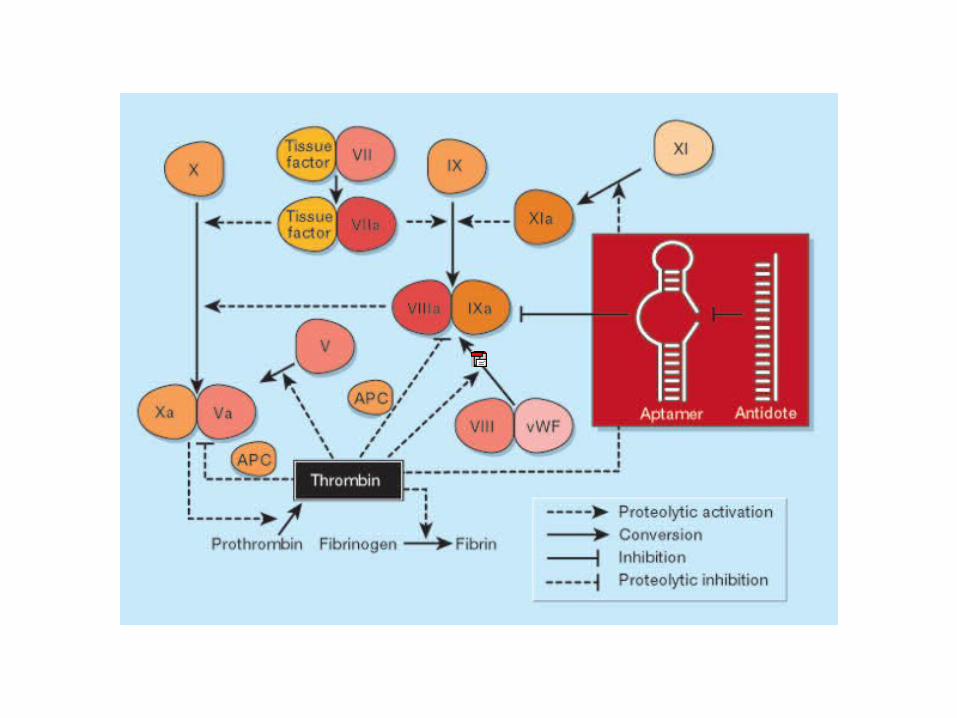
RNA functions

• RNA functions as– mRNA– rRNA– tRNA– Nuclear export– Spliceosome– Regulatory molecules (RNAi)– Enzymes– Virus– Retrotransposons– Medicine

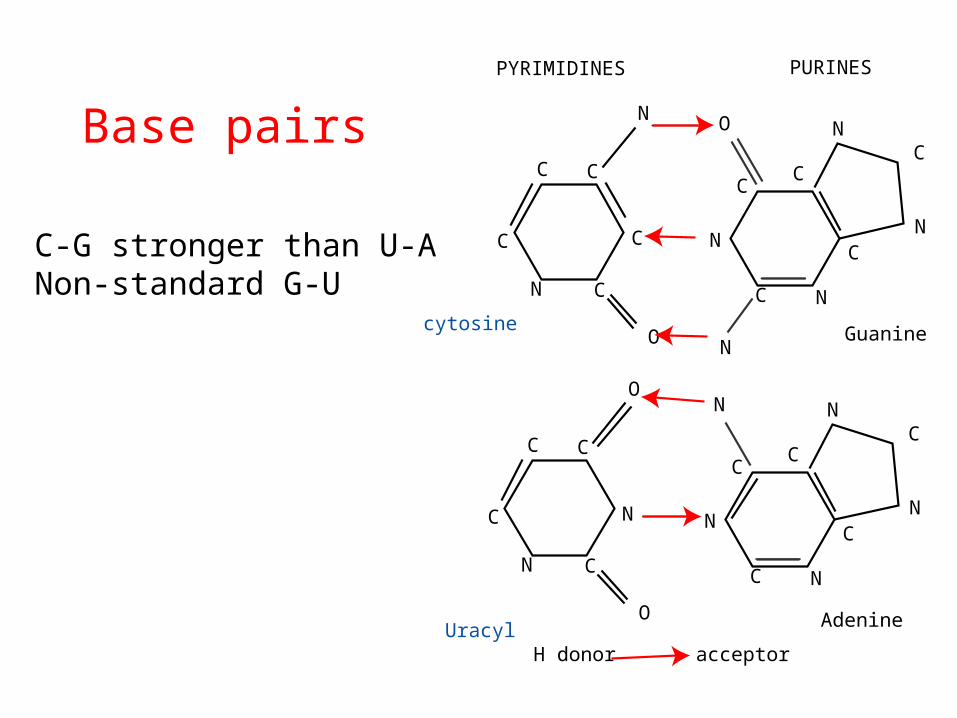
Base pairs

• C-G stronger than U-A• Non-standard G-U

CC

C

N

N C

O

C

CC

C

O

N C

O

N

cytosine

Uracyl

N

CC

C

NC

NC

N

N

O

N

CC

C

NC

NC

N

N

Adenine

Guanine

PYRIMIDINES PURINES

H donor acceptor

• Base-pairs are usually coplanar

• are almost always stacked

• stems – continuous stacks

• 3D structure of a stack is a helix

hairpin

Stacking

Predictable structures

Hard-to-predict structures

• Pseudoknots, kissing hairpins, hairpin-bulge

Secondary structure notations

Structure representation

Tertiary structure

RNAi

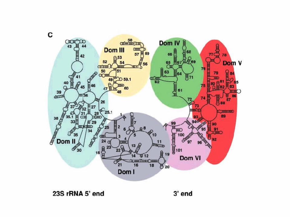
Known RNA Structureshttp://www.rnabase.org/metaanalysis/ httpp://www.sanger.ac.uk/Software/rfam http://www.scor.lbl,gov

Rfam – database of RNA alignments and secondary structure models

Scor - database of RNA experimentally solved structures

Main approaches to RNA secondary structure prediction

• Energy minimization – dynamic programming approach– does not require prior sequence alignment– require estimation of energy terms

contributing to secondary structure

• Comparative sequence analysis– Using sequence alignment to find conserved

residues and covariant base pairs.– most trusted

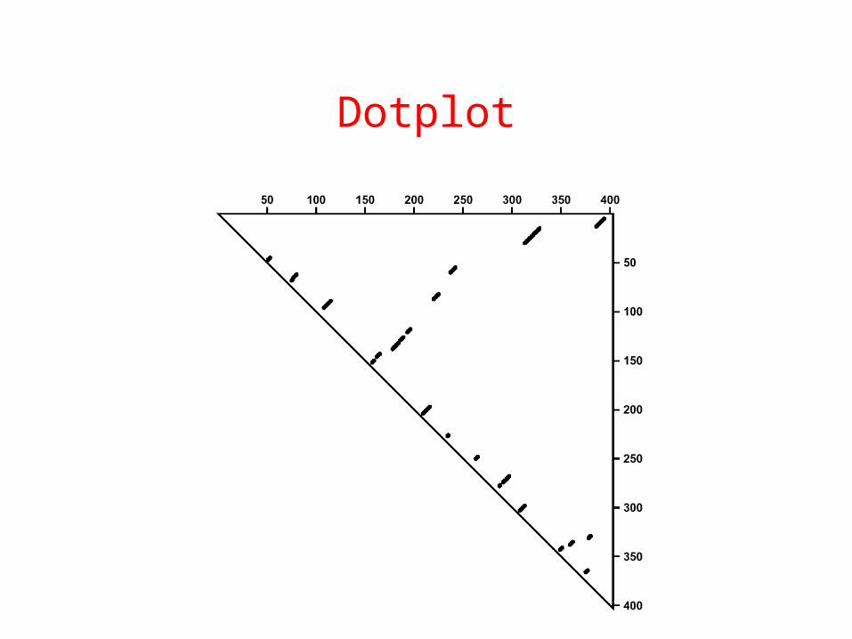
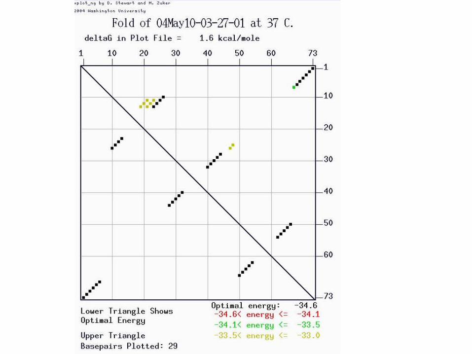
Dotplot

Think!

• Make a dotplot of an RNA molecule– Sequence : GGGAAAUCC

• What is the secondary structure?

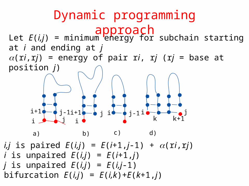
Dynamic programming approach

• Nussinov algorithm

Dynamic programming approach

a) i,j is paired E(i,j) = E(i+1,j-1) + (ri,rj)b) i is unpaired E(i,j) = E(i+1,j) c) j is unpaired E(i,j) = E(i,j-1)d) bifurcation E(i,j) = E(i,k)+E(k+1,j)

i+1 j-1 i+1 j ji j-1i j i

ik k+1

a) b) c) d)

Let E(i,j) = minimum energy for subchain starting at i and ending at j(ri,rj) = energy of pair ri, rj (rj = base at position j)

RNA secondary structure algorithm

• Given: RNA sequence x1,x2,x3,x4,x5,x6,…,xL

• Initialization: E(i, i-1) = 0 for i = 2 to LE(i, i) = 0 for i = 1 to L

Recursion: for n = 2 to L # iteration over length

E(i,j) = min { E(i+1, j), E(i, j-1), E(i+1, j-1)+ (ri,rj) ,

min i<k<j {E(i,k)+E(k+1, j)} }

• Cost: O(n3)

ExampleLet (ri,rj) = -1 if ri,rj form a base pair and 0 otherwise Input : GGAAAUCC

G G A A A U C C

G 0

G 0 0

A 0 0

A 0 0

A 0 0

U 0 0

C 0 0

C 0 0

E(i,j) = lowestenergy conformation for subchain from i to j

i

j

Here we should have min energy for AAAUC

Example-continued

G G A A A U C C

G 0 0

G 0 0 0

A 0 0 0

A 0 0 0

A 0 0 -1

U 0 0 0

C 0 0 0

C 0 0

GGA (i=2, j=3)min { 0,

0,0+ (GA)

} = 0

AAU (i=5, j=6)min { 0,

0,0+ (AU)

} = -1

-1

0

i

j

Recovering the structure from the DP table

Main difference to sequence alignment – we are tracing back a tree-like structure not a single optimal path (bifurcation introduces branch points).

Method 1: Leave pointers as you compute the table: for each element of the table store (at most two) pointers to the subsequences used in the solution.

Method 2: Recover history based on numerical values in the table.Stacking – check value along diagonalBifurcation - find k such that E(i,k)+E(k+1,j) =

E(i,j)

• Base-pairs are usually coplanar

• are almost always stacked

• stems – continuous stacks

• 3D structure of a stack is a helix

hairpin

Stacking

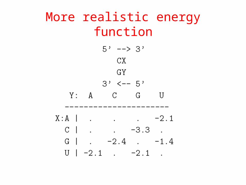
More realistic energy function

Stacking energies

Covariance method

In a correct multiple alignment RNAs, conserved base pairs are often revealed by the presence of frequent correlated compensatory mutations.

Two boxed positions are covarying to maintain Watson-Crick complementary. This covariation implies a base pair which may then be extended in both directions.

GCCUUCGGGCGACUUCGGUCGGCUUCGGCC

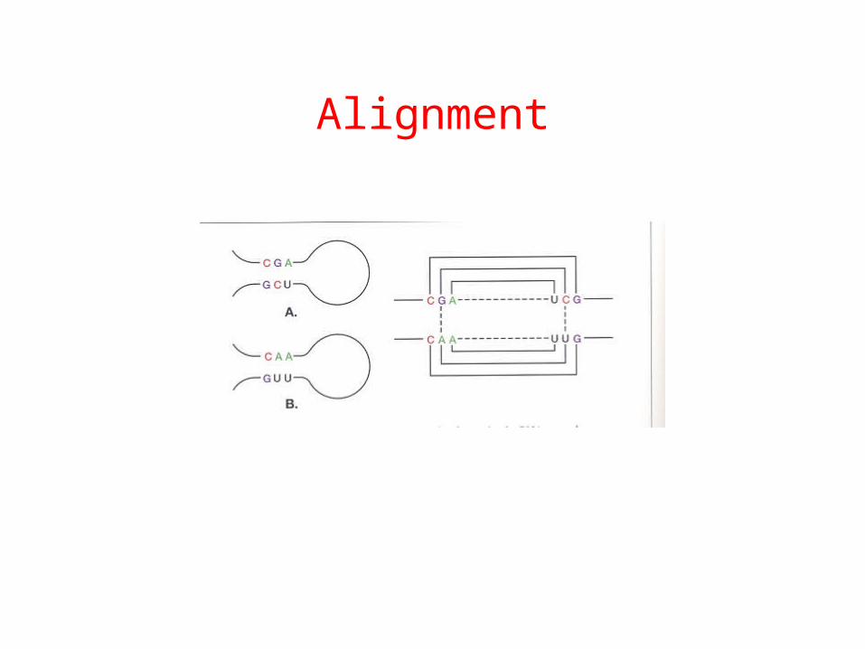
Alignment

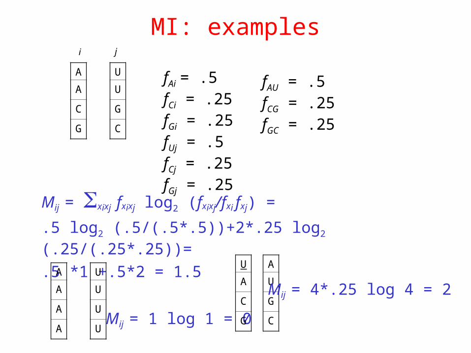
Measure of pairwise sequence covariation

Mutual information Mij between two aligned columns i, j

Mij = i,j fxixj log2 (fxixj/fxi fxj)where fxixj frequency of the pair (observed)

fxi frequency of nucleotide xi at position i

Observations: 0 <= Mij <=2

i,j uncorrelated Mij = 0

MI: examples

A

A

C

G

U

U

G

C

fAi = .5fCi = .25fGi = .25fUj = .5fCj = .25fGj = .25

fAU = .5fCG = .25fGC = .25

Mij = xixj fxixj log2 (fxixj/fxi fxj) =

.5 log2 (.5/(.5*.5))+2*.25 log2 (.25/(.25*.25))=

.5 *1 +.5*2 = 1.5A

A

A

A

U

U

U

UMij = 1 log 1 = 0

U

A

C

G

A

U

G

C

Mij = 4*.25 log 4 = 2

i j

Other methods

• HMMs• Stochastic context free grammars

• Allow for modeling complex structures.

• Allow incorporation of additional info:– Phylogenetic distances– Biochemical properties

sno-RNA HMM

Stochastic Grammars

S -> aSa -> abSba -> abaaba

i. Start with S. Production rules:S --> (0.3)aT (0.7)bS T --> (0.2)aS (0.4)bT (0.2)

S -> aT -> aaS –> aabS -> aabaT -> aaba

ii. S--> (0.3)aSa (0.5)bSb (0.1)aa (0.1)bb

*0.3

*0.3 *0.2 *0.7 *0.3 *0.2

*0.5 *0.1

Derivation:

Conclusion

• RNA secondary structure prediction– Single sequence:

• Dot-plot• Nussinov dynamic programming• Energy function

– Covariance analysis• Mutual information• Hidden Markov Models • SCFGs