RNA-Seq Preparation Comparision Summary: Lexogen, Standard,

NEB

CSF-NGS

January 22, 2014

Contents

1 Introduction 1

2 Experimental Details 1

3 Results And Discussion 13.1 ERCC spike ins . . . . . . . . . . . . . . . . . . . . . . . . . . . . . . . . . . . . . . . . . . . . 13.2 RNA alignment . . . . . . . . . . . . . . . . . . . . . . . . . . . . . . . . . . . . . . . . . . . . 73.3 Differential Expression . . . . . . . . . . . . . . . . . . . . . . . . . . . . . . . . . . . . . . . . 11

1 Introduction

It was necessary to establish a quick but reliable protocol for the preparation of Illumina sequencing librarieswith total RNA as starting material to offer as a service for the CSF-NGS users. The current in houseprotocol (”standard”) was deemed as taking too long, because hands on time is the major cost factor. Manydifferent protocols and kits for mRNA preparation are currently available. (citations).

2 Experimental Details

Liver (Clontech cat. nr 636603) and Kidney (Clontech cat. nr 636612) mouse total RNA was used as sourcematerial. ERCC spike ins 1 or 2 (life-Technologiesi catalog number 4456740) were added to each source tubeand the combined sample was split to triplicates and each triplicate was prepared separately with eitherthe in-house standard protocol (std), the lexogen sense kit (lexogen catalog number 001.08) or the NEB kit(NEBNext Ultra Directional RNA Library Prep Kit for Illumina, catalog number E7420). The resultingsamples were sequenced on a HiSeq2000 SE with a read length of 50. The reads were 5’ trimmed for thelexogen preparation method, adaptors were removed with cutadapt, the rRNA reads and ERCC spike inswere removed by alignment with bowtie, and the remaining reads were aligned to the mouse mm10 genomeand transcriptome using tophat 1.4.1. The aligned tophat reads were counted per gene with HTSeq-countand the counts were used for differential gene expression estimation using DESeq.

3 Results And Discussion

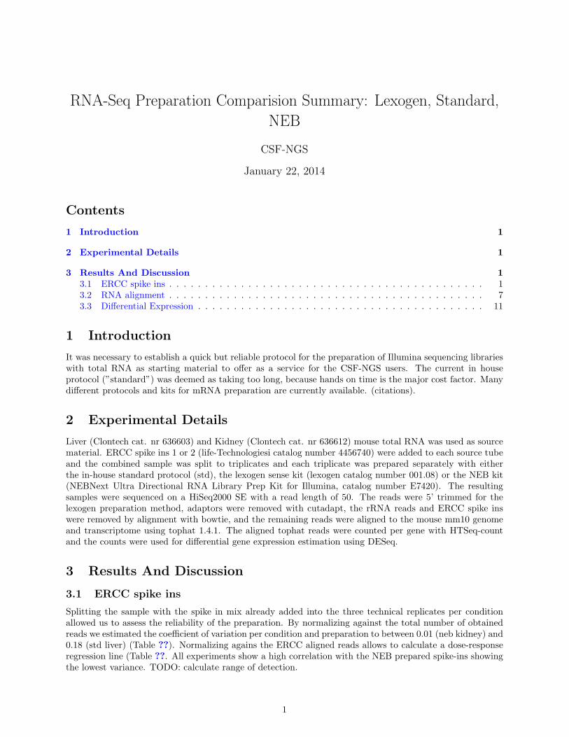
3.1 ERCC spike ins

Splitting the sample with the spike in mix already added into the three technical replicates per conditionallowed us to assess the reliability of the preparation. By normalizing against the total number of obtainedreads we estimated the coefficient of variation per condition and preparation to between 0.01 (neb kidney) and0.18 (std liver) (Table ??). Normalizing agains the ERCC aligned reads allows to calculate a dose-responseregression line (Table ??. All experiments show a high correlation with the NEB prepared spike-ins showingthe lowest variance. TODO: calculate range of detection.

1

Table 1: summary of results

Criteria Lexogen NEB Standard

hands on timea 5-6h 1d 3ddetection of differential gene expression very good very good very goodvariance per gene low very low lowstrandiness very high high highvariance of gene coverage spikyb very low very low5’ coverage lag low detectable detectablerRNA depletionc exhaustive low lowease of automatication not known protocols availabled lowduplication mediumb very low lowdynamic range good good gooda including RNA QC, excluding library QCb expected due to priming method, no influence on differential expressionc only one round of poly-A enrichmentd for Hamilton STAR robot

2

prep condition mean sd cvstd liver 0.44 0.08 0.18std kidney 0.49 0.03 0.07lex liver 0.57 0.04 0.06lex kidney 1.31 0.08 0.06neb liver 0.68 0.04 0.06neb kidney 0.77 0.01 0.01

●

●

●

●

●

●

0.6

0.9

1.2

std lex nebprep

perc

ent E

RC

C/to

tal replicate

● 1

2

3

condition

●

●

liver

kidney

Figure 1: Relative abundance of ERCC-Spike Ins compared to total number of reads. Reads were alignedwith bowtie against the ERCC genes and the mouse rDNA cluster and the uniquely aligning reads werecounted.

3

prep condition intercept slope R2std liver 1.03 0.861 0.864std kidney 0.806 0.877 0.888lex liver 0.967 0.905 0.899lex kidney 1.01 0.892 0.893neb liver 0.607 0.931 0.96neb kidney 0.384 0.948 0.966

std lex neb

0

5

10

15

20

0

5

10

15

20

liverkidney

−5 0 5 10 15 −5 0 5 10 15 −5 0 5 10 15log2(expected attomoles)

log2

(rpk

m)

legend

expected

lm

loess

ND

Figure 2: ERCC dose response. The sum of all the uniquely aligning reads per ERCC gene was normalized bythe length of the gene and the total number of reads aligning uniquely to the ERCC controls and the resultingrpkm values were plotted against the expected number of RNA-molecules. Linear regression parameters (top)and scatter plot (bottom) with expected counts (blue line), regression line (red line), loess curve (green line)and undetected genes at an arbitrary rpkm value (yellow dots).

4

std lex neb

y = 0.13+ 0.9⋅ x

r 2 = 0.691

y = −0.056+ 1 ⋅ x

r 2 = 0.77

y = 0.0023+ 0.97⋅ x

r 2 = 0.801

−2

0

2

−1 0 1 2 −1 0 1 2 −1 0 1 2expected log2(l/k)

log2

(l/k) model

expected

lm

Figure 3: ERCC fold-change response. The ratios of the mean rpm log2 ratio per condition were plottedagainst the expected log2 ratio. Expected counts (red line) and regression line (green line) are indicated.

5

0

10000

20000

30000

0

1000

2000

3000

0

200

400

600

0

5

10

15

(0,5](5,10]

(10,20](20,92]

0 25 50 75 100position %

aver

age

cove

rage

per

mill

ion

read

s

prep

std

lex

neb

Figure 4: ERCC coverage across genes. The genes were binned per preparation method by their rank (top 5,6-10, 11-20, rest) and the average coverage per million reads per bin is plotted against the length normalizedgenes.

6

3.2 RNA alignment

7

stdliver

stdkidney

lexliver

lexkidney

nebliver

nebkidney

0e+00

1e+07

2e+07

3e+07

1595

6

1595

7

1595

8

1595

9

1596

0

1596

1

1596

9

1597

0

1597

1

1597

2

1597

3

1597

4

1615

3

1615

4

1615

5

1615

6

1615

7

1615

8

sample id

abso

lute

cou

nts

V1

Cleaned

Cut

NM

R

U0

U1

U2

std lex neb

●

●

●●●

●

●

●

●

●●

●

●

●

●

●

●

●

●●●

●

●

●

●

●

●

●

●

●

●

●

●

●

●

●

●

●●●

●

●0

20

40

60

Cle

aned Cut

NM R U0

U1

U2

Cle

aned Cut

NM R U0

U1

U2

Cle

aned Cut

NM R U0

U1

U2

align type

perc

ent o

f tot

al

replicate

● 1

2

3

condition

●

●

liver

kidney

Alignment Distribution

Figure 5: Alignment Statistics. The reads were 5’ trimmed for the lexogen preparation method, adaptorswere removed with cutadapt, the rRNA reads and ERCC spike ins were removed by alignment with bowtie,and the remaining reads were aligned to the mouse mm10 genome and transcriptome using tophat 1.4.1.Absolute counts (top panel) and relative percentage (bottom panel) of each alignment category (Cut: smalladaptor truncated reads removed, Cleaned: reads aligning to ERCC or rRNA, U0-U3: unique alignmentswith 0-3 mismatches, R: reads aligning repetitively, NM: reads not aligning) are shown.

8

0

25

50

75

100

10 1000X−plicates

cum

ulat

ive

perc

ent o

f uni

quel

y al

igne

d re

ads

preparation

lex

neb

std

replicate

1

2

3

Figure 6: Xplicates. Uniquely aligned reads were binned by number of overlaps at each position and thecumulative sum was calculated with increasing number of duplication.

9

unstranded same opposite

0.0

0.5

1.0

1.5

0.0

0.5

1.0

1.5

0.0

0.5

1.0

1.5

lexneb

std

0 25 50 75 100 0 25 50 75 100 0 25 50 75 100bin

norm

aliz

ed m

ean

cove

rage condition

kidney

liver

replicate

1

2

3

Figure 7: Coverage across cDNA. Mean coverage across all length normalized genes (cDNA).

10

3.3 Differential Expression

11

Scatter Plot Matrix

std0

5

0 5

−10

−5

−10 −5

0.93 0.95

lex0

5

100 5 10

−10

−5

0

−10 −5 0

0.95

neb0

5

100 5 10

−10

−5

0

−10 −5 0

Figure 8: Scatter plot matrix of log2 fold changes per preparation. The log2 fold changes of the comparisonliver/kidney of each preparation were plotted against each other (upper triangle) and the spearman rankcorrelation was calculated (lower triangle).

12

lex k

lex l

neb k

neb l

std k

std l

1e−0

4

1e−0

2

1e+0

0

1e+0

11e

+03

1e+0

51e

+01

1e+0

31e

+05

1e+0

11e

+03

1e+0

51e

+01

1e+0

31e

+05

1e+0

11e

+03

1e+0

51e

+01

1e+0

31e

+05

mea

n

dispersion

Fig

ure

9:T

heva

rian

ceof

each

cond

itio

nw

ases

tim

ated

byde

seq

esti

mat

eDis

pers

ions

wit

hth

em

odel

fitin

dica

ted

inre

d.

13

lexneb

std

adj.p < 0.01 ; abs(log2FC) > 1

std 6025 lex 6170 neb 6434

lex

nebstd

adj.p < 0.01 ; abs(log2FC) > 5

std 1180 lex 1190 neb 1258

lex

neb

std

adj.p < 0.001 ; abs(log2FC) > 5

std 1127 lex 1155 neb 1215

lex

neb

std

adj.p < 0.001 ; abs(log2FC) > 10

std 169 lex 194 neb 392

Figure 10: Venn Diagrams of significantly differentially expressed genes under different cutoffs.

14