RIVM rapport 680740003 STAMINA-Model description · STAMINA-Model description ... within the...

Report 680740003/2010

E.M. Schreurs | J. Jabben | E.N.G. Verheijen

STAMINA-Model descriptionStandard Model Instrumentation for Noise Assessments

RIVM Report 680740003/2010

STAMINA - Model description Standard Model Instrumentation for Noise Assessments

E.M. Schreurs J. Jabben E.N.G. Verheijen Contact: Eric Schreurs Centre for Environmental Monitoring [email protected]

This investigation has been performed by order and for the account of Ministry of Housing, Spatial Planning and the Environment (VROM DGM-LOK), within the framework of project ‘Monitoring Geluid’, project number M/680740/08/SB

RIVM, P.O. Box 1, 3720 BA Bilthoven, the Netherlands Tel +31 30 274 91 11 www.rivm.nl

© RIVM 2010 Parts of this publication may be reproduced, provided acknowledgement is given to the 'National Institute for Public Health and the Environment', along with the title and year of publication.

RIVM Report 680740003 2

Abstract STAMINA - Model description Standard Model Instrumentation for Noise Assessments This report describes the STAMINA model (Standard Model Intrumentation for Noise Assessments), which was developed at RIVM. The instrumentation is used to map environmental noise in the Netherlands. The STAMINA model implements the standard Dutch Calculation method for traffic and industrial noise, which is used in the Netherlands to implement the European Environmental Noise Directive. The STAMINA model is used to support and advise the Ministry of Housing Spatial Planning and the Environment in developing new noise policies and noise legislation. The STAMINA model can be used to create noise maps, showing the noise levels due to traffic and industrial noise. These noise maps can be consulted online (http://www.rivm.nl/milieuportaal/onderwerpen/geluid/geluidbelasting/), yet can not be used to examine the noise legislation. Combining the noise produced by road-, railway-, air traffic and industrial noise, an overall picture of the noise exposure in the Netherlands can be made. The noise levels are shown in Lden. This noise indicator averages the noise produced in one day, with penalties for noise produced in the evening and nighttime. The Lden indicator is standardized in the EU. Key words: noise, monitoring, decibel, industrial noise, roadway traffic


Rapport in het kort STAMINA – Model beschrijving Standard Model Instrumentation for Noise Assessments Deze rapportage beschrijft het STAMINA-model, dat staat voor Standard Model Instrumentation for Noise Assessments en door het RIVM is ontwikkeld. Het instituut gebruikt dit standaardmodel om omgevingsgeluid in Nederland in kaart te brengen. Het model is gebaseerd op de Standaard Karteringsmethode voor verkeerslawaai en industrielawaai, die in Nederland is voorgeschreven om de Europese richtlijn voor omgevingslawaai uit te voeren. Met het STAMINA-model ondersteunt het RIVM beleid over en monitoring van omgevingsgeluid voor het ministerie van VROM. Het STAMINA-model levert data waarmee geluidkaarten worden gemaakt. Deze kaarten geven een beeld van de geluidbelasting. De kaarten zijn online beschikbaar (http://www.rivm.nl/milieuportaal/onderwerpen/geluid/geluidbelasting/), zodat geïnteresseerden op postcodeniveau een beeld kunnen krijgen van de geluidbelasting in hun omgeving. De kaarten zijn niet geschikt om wettelijke normen voor geluid te toetsen. Door kaarten met uiteenlopende informatie over geluid samen te voegen, bijvoorbeeld van vliegverkeer, wegverkeer en spoorwegen, kan een totaalbeeld geschetst worden van de geluidbelasting in heel Nederland. De geluidbelasting wordt aangeduid met de eenheid Lden. Deze indicator geeft weer wat de geluidbelasting gemiddeld over een dag is. Hij maakt daarbij onderscheid tussen de waarden van de dag, avond en nacht en geeft deze waarden vervolgens gecombineerd en gewogen weer. Lden wordt in de Europese Unie als standaard gebruikt. Trefwoorden: geluid, monitoring, decibel, wegverkeer, industrielawaai


Contents

Summary 6

1 Introduction 8 1.1 General 8 1.2 STAMINA 8

2 Standard methods for noise mapping 9 2.1 European noise indicator Lden 9 2.2 SRM-methods for road and railway traffic 9 2.3 Industrial sources 10 2.4 Upgrade of SRM into SKM 10

3 Implementation of SKM into STAMINA 12 3.1 Layout of the noise maps 12 3.2 Mapping of the road and railways 13 3.3 Ground attenuation 15 3.4 Source data 16 3.4.1 Roadway traffic 16 3.4.2 Railway traffic 17 3.4.3 Industrial noise 17 3.4.4 Wind turbines 18

4 Validation 20 4.1 Noise propagation 20 4.2 Spectral validation 21 4.3 Urban environment 22 4.4 Comparison with EU data 23

5 Noise maps and applications 25 5.1 Noise maps 25 5.1.1 Roadway traffic 25 5.1.2 Railway traffic 26 5.1.3 Industrial noise 27 5.1.4 Cumulative noise map 28 5.2 Applications and discussion 29 5.2.1 Current applications 29 5.2.2 Uncertainties and future developments 29

References 30

Appendix A: Examples of Ascii input data used by STAMINA 33


Summary

The STAMINA model The STAMINA model (Standard Model Instrumentation for Noise Assessments), is developed at the National Institute for Public Health and the Environment (RIVM), and is an instrumentation tool in order to map environmental noise in the Netherlands. The STAMINA model implements the standard Dutch Calculation method for traffic and industrial noise, which is used in the Netherlands to implement the European Environmental Noise Directive. The STAMINA model is used to support and advise the Ministry of Housing, Spatial Planning and the Environment in developing new noise policies and noise legislation.

Implementation Calculations of noise caused by road-, railway traffic and industrial noise in the Netherlands are done according to the standardized Dutch calculation methods (‘Standaard Rekenmethoden’, or SRM). These methods are laid down by the Dutch Noise legislation, the ‘Wet Geluidhinder’, and are well documented (VROM, 2006a/b). The SRM method was originally designed for single point calculations from the source to one or a limited number of receiver points, where the noise level is to be compared with limit values. In order to use these methods for large scale noise mapping, STAMINA has upgraded the SRM method into the standard Dutch ‘Standaard Karteringsmethode’, or SKM-method. Subsequently, the STAMINA model implements the SKM method in order to produce noise maps. This is done using detailed information of the noise source types (roadway traffic, railway traffic, industrial noise, wind turbines) and ground use data. The extent of detail of the noise maps depends on the distance between source and observation point; the lowest resolution is 80 x 80 m, and close to the source the level is detailed is highest, with a resolution of 10 x 10 m.

Validation To verify if the STAMINA model implements the SRM method correctly, it has been compared with a different model which implements the SRM2 method. This model was the ‘Winhavik’ model, and the results of the comparison for situations with and without a noise barrier are shown in Figure 1.

30

40

50

60

70

80

10 100 1000 10000 100000Distance [m]

L Aeq

[dB

]

STAMINA: no barrier SRM2: no barrier

STAMINA: 4m barrier SRM2: 4m barrier

Hard surface

30

40

50

60

70

80

10 100 1000Distance [m]

L Aeq

[dB

]

Absorbent surface

Figure 1: Noise immission as a function of the distance. Comparison between STAMINA and SRM2 model.


In the situation without a barrier there is only a negligible difference. The small deviations may be caused by the model parameters like aperture angle (‘sectorhoek’) and by rounding. It is remarked here that most of the practical situations with a barrier will involve dwellings close to the road (25 m – 50 m) while the average difference between STAMINA and SRM2 in this range appears to be nearly zero.

Results Combining the noise maps for roadway traffic, railway traffic, industrial noise and wind turbine noise, a cumulative noise map of the Netherlands can be made, which gives an indication of the overall noise exposure in the Netherlands. This is shown in Figure 2, which also contains data on airport noise provided by the National Aerospace Laboratory. The noise levels are shown in Lden. This noise indicator averages the noise produced in one day, with penalties for noise produced in the evening and nighttime. The Lden indicator is standardized in the EU.

Figure 2: Cumulative noise map of the Netherlands.


1 Introduction

1.1 General

The Centre of Environmental Monitoring at RIVM supports governmental noise policies by global noise studies that are aimed at monitoring noise exposure and evaluation of noise measures. The noise exposure of the Dutch population and the effectiveness of noise policies must be assessed taking into account all regions of interest i.e. the noise exposure must be evaluated at all dwellings in the Netherlands and for all source types that are known to cause annoyance effects on the population. To this aim noise maps are set up, based geographical input data containing the locations and activities of the sources. The noise maps are combined with geographical databases containing the number and locations of the dwellings involved in order to evaluate effects. The noise maps are used to asses the impact of noise on dwellings and inhabitants, sanctuaries and nature areas. By updating the underlying input data, the maps are kept up to date and serve as a monitoring tool. Also the maps are used to study the effects of noise control measures and to evaluate their effectiveness on a national scale. The results are used to support and advise the Ministry of Housing, Spatial Planning and the Environment in developing new noise policies and noise legislation.

1.2 STAMINA

The connection between the source input data (roads, railways, industrial areas and wind turbines) and the noise maps is provided by STAMINA (Standard Model Instrumentation for Noise Assessments). STAMINA is a grid based noise model implemented in C++ software, which uses the Dutch standard SKM-method for noise mapping. This report describes the STAMINA noise mapping tool developed at the Centre for Environmental Monitoring (CMM) of RIVM, for setting up detailed noise maps on a national scale. It contains an extensive explanation of the noise mapping methods used for environmental noise from road- and railway traffic, industrial sources and wind turbines. Chapter 2 deals with the Dutch National Standard for noise mapping used in the Netherlands. Chapter 3 gives an extensive description of the implementation of the SKM method into the mapping tools that are used for setting op the noise grids. In chapter 4 the results for different types of noise sources are validated. Chapter 5 shows the resulting noise maps, and finally applications, limitations and uncertainties are discussed.


2 Standard methods for noise mapping In 2002 directive 2002/49/EC of the European parliament and of the council of 25 June 2002 was issued, relating to the assessment and management of environmental noise. This European directive obliges Member States to assess the noise situation in the main urban agglomerations and set up action plans to reduce environmental noise at dwellings with high noise exposure. In order to obtain a complete picture of noise exposure, Member States have to set up noise maps using the European standard Lden noise indicator. Although it is envisaged to harmonize the methods that are used to calculate noise levels and set up the noise maps, an official European standardized method for noise mapping is still not available. In the Netherlands, the standard methods (‘Standaard Rekenmethoden’, SRM) for noise from road- (VROM, 2006a) and railway traffic (VROM, 2006b) were upgraded into the ‘Standaard Karteringsmethode’ (SKM) in order make the SRM methods suitable for noise mapping. The SKM method is now used by RIVM to set up noise maps on a national scale. These methods are briefly outlined here. For a detailed description see (CROW, 2004).

2.1 European noise indicator Lden

A harmonized European noise indicator is the Lden. This noise indicator uses a time weighted average of equivalent noise levels over 24 hours. It is defined according to:

⎟⎟⎠

⎞⎜⎜⎝

⎛⋅+⋅+⋅=

++

1010

105

10,,,

1024810

24410

2412log10

nightAeqeveningAeqdayAeq LLL

denL (2.1)

As equation 2.1 shows, the Lden averages the equivalent noise levels produced in the day (7.00 – 19.00), evening (19.00 – 23.00) and night (23.00 – 7.00) periods after penalizing. As noise produced in evening and night time periods cause generally more annoyance, penalties are added to these noise levels. These penalties are 5 dB for noise produced in the evening period, and 10 dB for the night period.

2.2 SRM methods for road and railway traffic

By standard, local calculations of noise caused by road- or railway traffic in the Netherlands are done according to the standardized Dutch calculation SRM methods for road- and railway traffic. These methods are laid down by the Dutch Noise legislation, the ‘Wet Geluidhinder’, in order to determine noise levels that can be checked against legal limits (VROM, 2006a). The SRM methods consist of two methods: a simple version called Method 1, and Method 2 which should be applied in more complex situations. Equation 2.2 gives the basic equation from SRM2 for the calculation of road traffic noise. The road is split up in subsegments, as shown in Figure 2.1, for which each contribution at the receiver is determined separately:

6.58,,,,,, −−−−−−= MeteoiBarrieriGroundiAiriGeoiEiden CAAAALL (2.2)

in which the Lden is the noise level at the observation point. LE is the noise emission of the source and the ‘A’-terms denote the attenuation from source to receiver due to geometric spreading (AGeo), air


absorption (Aair), ground impedance (Aground) and Noise Barriers. The index i runs over eight octave band numbers, with centre frequencies ranging from 63 Hz up to 8 kHz. CMeteo is a frequency independent meteorological correction accounting for varying wind directions and temperature gradients. The constant of 58.6 dB is a correction for dimension changes. The noise emission LE for road traffic depends on the surface type of the road, traffic speed and the intensity of each type of vehicle (which is differentiated into light, medium-heavy and heavy vehicles) during each part of the 24 hours (day, evening and night). A similar equation is used for railway noise, where the emission term depends on railway stock, speed and superstructure (VROM, 2006b).

Figure 2.1: Illustration of road segmenting used in SRM2. Figure 2.1 shows how the traffic line from A to B is cut in four segments. For each segment, the noise propagation between the segment and the receiver is considered along the bisector, indicated by the dotted lines in Figure 2.1. Subsequently for each bisector and frequency band equation 2.1 is applied in order to calculate its contribution to the total sound level at the receiver point R. For further information the manual of the Dutch standard calculation method can be consulted (VROM, 2006a/b).

2.3 Industrial sources

For industrial sources in the Netherlands the standard method is given in (VROM, 2006c). It differs from the standard methods for road and railway traffic in the sense that emission and propagation factors are specified for point sources in stead of line segments. The basic formula for the propagation is in general the same as equation 2.2, with the exception that the source term LE are point sources instead of line sources. For global noise maps on a national scale, source terms are estimated for large industrial areas as discussed in section 3.4.3. The Dutch standard calculation method for noise from industrial sources is also used for setting up noise maps for wind turbine noise.

2.4 Upgrade of SRM into SKM

The ‘Standaard Rekenmethoden’ (SRM) were originally designed for single point calculations from the source to one or a limited number of receiver points, where the noise level is to be compared with limit

R

BA 2 34

1


values. In order to use these methods for large scale noise mapping, the SRM methods were upgraded into the standard Dutch SKM method. The upgrade consists of a detailed specification of the way that buildings between source and receiver have to be taken into account, by adding an extra attenuation factor ASKM to equation 2.2. This term treats buildings between the source and receiver position as noise barriers, and the amount of attenuation depends on the amount of buildings present. For a detailed description Section 6.3 of (CROW, 2004) can be consulted.


3 Implementation of SKM into STAMINA This chapter describes how the standard SKM model outlined the previous chapter has been implemented in STAMINA. STAMINA is a C++ software program that sets up complete noise maps for road and railway traffic covering the Netherlands. In this chapter first a description is given of the software implementation and subsequently the data forms used to create the maps are outlined.

3.1 Layout of the noise maps

Using the standard SKM method outlined in the previous chapter, for each of the described sources a C++ program was developed. The software calculates Lden noise levels on a 10 x 10 m grid covering the Netherlands in according to (WGAEN, 2007). The coordinates are based on the ‘Rijksdriehoekmeting (RD)’ system, and the RD coordinates of the lower left corner are (14000,307000) and of the upper right (278000,619000). In view of limited memory, the grid is divided into 2288 subgrids of 6 x 6 km2, each containing 360,000 gridpoints. The layout is given in Figure 3.1

Figure 3.1: Noise mapping area (264 x 312 km2) for the Netherlands, divided in 2288 subgrids each of 6 x 6 km2. Gridsize 10 x 10 m2. Each subgrid contains 360,000 gridpoints, for which the Lden noise level is determined.


Noise levels are the calculated for each subgrid successively. At the start of a new subgrid the program runs through a list of input. Only those sources that are located in the subgrid or within 4 km of its boundary are taken into account and contribute to the noise levels. After all points of the subgrid are calculated, the program stores the data in a temporary (ascii) outputgrid and proceeds to the next subgrid, until the complete grid is covered. After finishing, all outputgrid are merged into one large Acii-gridfile that is converted into ARC-GIS format and used for further analysis.

3.2 Mapping of the road and railways

For each subgrid, the model looks through databases containing the road- and railways in the Netherlands in order to determine which road- or railways are located within the subgrid. These databases are discussed in chapter 4. Subsequently the road- and railways in the subgrid are divided into segments. These segments have a maximum length of 250 m for motorways and railways, and 100 m for municipal roads. An illustration of the mapping process for such a segment is depicted in Figure 3.2.

Figure 3.2: The STAMINA mapping procedure for a single noise segment within the region (R) of interest. For the segment indicated by the yellow line a rectangular envelope is defined, extending R km around the segment. This is indicated by the yellow area in Figure 3.2, and is called the region of interest. The length of R depends on the type of the source: noise emissions from motorways and railways are generally higher than from municipal roads, and correct noise mapping requires a larger region of interest than noise from municipal roads. The length is varied as shown in Table 3.1.

A i

R

80 m

B


The mapping program steps through the yellow area using a grid of 80 x 80 m, following the path A to B. This is the ‘stepping grid’, indicated with the black squares in Figure 3.2. It contains 64 square grid cells of width 10 m. At each centre point (i) the noise contribution of the segment is determined using equation 2.2 and dividing the segment into subangles of 15 degrees. In this way the yellow area is completely covered. Based on the distance between the centre of the stepping grid and the road segment it is decided whether this distance is large enough so that the noise level at the centre be attributed to all 10 m cells in the stepping grid. If this is not the case, a refinement is needed and the stepping grid is divided into smaller grids of at least 10 m. The latter is the case when the stepping grid centre of is nearer to the noise source (segment), as noise levels tend to have more spatial variation there. Therefore the model has a resolution of 10 x 10 m close to the source segment. When the observation point is further away from the segment, this resolution gradually increases to at most 80 x 80 m. For the different types of road and railways, the criteria are chosen as shown in Table 3.1: Table 3.1 Criteria for grid resolution for the different noise sources.

Source Region of interest length (R)

# Subdivisions of 80x80 m stepping grid

Distance from segment

Grid size

Main motorways 2800 m 64 0 – 100 m 10 x 10 m 16 100 – 300 m 20 x 20 m 4 300 – 800 m 40 x 40 m 0 800 – 2800 m 80 x 80 m Secondary 1500 m 64 0 – 100 m 10 x 10 m motorways 16 100 – 200 m 20 x 20 m 4 200 – 400 m 40 x 40 m 0 400 – 1500 m 80 x 80 m Municipal roads 500 m 64 0 – 100 m 10 x 10 m 16 100 – 200 m 20 x 20 m 4 200 – 400 m 40 x 40 m 0 400 – 500 m 80 x 80 m Railways 2000 m 64 0 – 100 m 10 x 10 m 16 100 – 200 m 20 x 20 m 4 200 – 400 m 40 x 40 m 0 400 – 2000 m 80 x 80 m

The resolution varies from 10 x 10 m up to 80 x 80 m, yet the ground data remains set at 10 x 10 m. Around the noise sources, in the case of road and railways, the resolution is at its highest (10 x 10 m). At increasing distances from the source, the resolution becomes 20 x 20, 40 x 40 and 80 x 80 m. At distances over R meter from the source, geometric spreading, air and ground absorption have attenuated the levels well below the natural background levels (around 30 dB) so that further calculations can be neglected. After all contributions of the segment on the grid cells within the yellow region are determined, the values are added to the grid contribution of previous segments and stored. In this way all segments are passed through, until the entire road or railway network has been put through. By this procedure the calculation times for large grids can be reduced considerably, without loss of quality, as at large distances noise levels vary relatively slowly and a resolution of 80 x 80 m is sufficient. The calculation time needed to process all 2288 subgrids ranges between 24 hours for the relatively small datasets (motorways, railways) and over 48 hours for the large datasets (secondary motorways and municipal roads).


3.3 Ground attenuation

In STAMINA, noise levels on grid points are calculated according to the basic attenuation terms from the Dutch Standard. For STAMINA, to take into account effect of the ground impedance (Aground, see equation 2.2) it needs ground data for the whole of the Netherlands divided in square cells of dimension 10 x 10 m. The ground data contains information for each gridcell regarding the ground impedance (water, grass, asphalt) and the presence of buildings. This information is provided according to the ground category classification specified in Table 3.2. Table 3.2 Ground classification codes used by STAMINA, available for each 10 x 10 m gridcell covering the Netherlands.

Ground classification Ground absorption Ground type Height of buildings 0 1 Grass, earth, sand, forest - 1 0.5 Partly asphalted - 2 0 Fully asphalted, water - 3 0 Buildings 8 m 4 0 Buildings 20 m

The first 3 categories denote the vacant areas in the Netherlands, and are distinguished only by their ground absorption properties. For instance, water and asphalt are assigned to category 2, denoting low sound absorption properties, whereas forests and agricultural areas have high sound absorption. Summarizing, ground use categories 0, 1 and 2 have a ground absorption fraction of 1, 0.5 and 0, respectively. These ground absorption fractions can for instance be found in (VROM, 1997), and are used to calculate AGround in equation 2.2. For built areas, the ground use categories 3 and 4 are used. They both have a ground attenuation factor of 0 (no ground absorption). The distinction between categories 3 and 4 is the height of the buildings, which are 8 m and 20 m, respectively. This information was obtained from (Kadaster, 2006). The height of the buildings is used by STAMINA in order to calculate the attenuation from buildings (ASKM in equation 2.2) according to (CROW, 2004). An example of the ground classification data is given in Figure 3.3 for the city of Amsterdam.


Figure 3.3: Illustration of the ground classification data in 10 x 10 m grid for the city of Amsterdam.

3.4 Source data

In order to use the model described in the previous sections and to set up noise maps, furthermore knowledge of the various noise source characteristics is needed. This information concerns the locations of roads and railways, traffic volumes and constellation, train numbers and stock passing by, speeds, locations of barriers et cetera. This section describes the data for roadway, railway traffic and industrial sources.

3.4.1 Roadway traffic The Dutch roadways are divided in three different categories: national motorways, provincial roads and municipal roads. For each of these categories traffic data is available, although the extent of the information differs.

1. Motorways: for motorways traffic data was provided by the Dutch road maintenance authority Rijkswaterstaat/DVS, who manages the data in the framework of the European directive 2002/49/EC. The most recent data is from 2006 and consists of digital information (ARC


INFO-shape files) containing Traffic volumes, speeds, type of road surface, location and height of noise barriers and walls for the entire motorway network in the Netherlands;

2. Secondary (provincial) motorways: the data contains basically the same information as for the main roads and stems from an inventory by RIVM of data available at the provinces in 2001.

3. Municipal roads: The traffic network data is based on a limited set of municipal data (‘VerkeersMilieuKaarten’, VMK files) which is dated from 2000 till 2005. Using a land covering network, containing information about the type of road, traffic volumes on the missing parts were estimated (Dassen et al., 2000). As for speeds, standard 50 km/h is assumed. There is no information on the type of road surface and a standard dense asphaltic concrete pavement is assumed on al municipal roads.

In Appendix A for each of the road types mentioned, an example is given of input ascii data as used by STAMINA.

3.4.2 Railway traffic For railway traffic, input data is used as provided by the Dutch track manager Prorail. This is the so-called ASWIN database from 2004 that contains railway stock noise emission data for the entire railway network in the Netherlands. This data was supplemented with high speed railway traffic, of which the service between Amsterdam and Rotterdam began in 2009. For an example of input data also see Appendix A.

3.4.3 Industrial noise Noise from various commercial and industrial activities is joined in the Dutch legislation as ‘Industrial noise’. As there is no database available that contains up to date and complete noise emission data, noise emission estimates will be used. To asses the noise emission globally, for these areas use is made of noise emission estimates per square meter. The noise emissions estimates from several industrial noise sources (M+P, 1991) are given in Table 3.3. The method as described cannot be used for accurate predictions of noise loads on specific locations. It does provide a tool for global assessments and estimate of the relative importance of this type of noise with respect to other forms of noise pollution.


Table 3.3 Noise emission estimates used for global assessment of noise impact of large industries. Category Industry Type Noise Emission

Estimate [dB(A)/m2] 1 Petrochemical 70 1 Shipyard 70 1 Offshore 70 1 Shunting-Yard 70 1 Chemical 68 2 Processing 65 2 Coal/Gravel/Ore Transhipment 65 2 Container Transhipment 65 2 Mixed Cargo Transhipment 65 2 Multi-Purpose Transhipment 65 2 Construction 65 2 Concrete/Asphalt Plant 65 3 Power Plants 61 3 Scrapyards 60 3 Gas Transhipment 58 4 Warehousing 55 4 Cleaning and Disposal companies 53

3.4.4 Wind turbines Data containing the locations of wind turbines was obtained from WindService Holland. This data etc For wind turbine noise, a different source model should be used as the noise emission from wind turbines depends on the generator power of the turbines Pelek, and on the wind speed at the hub height, as proposed by (Van den Berg et al., 2008). The exact dependence of the noise emission on the generator power was determined by fitting a logarithmic curve through the known sound power levels of 43 types of wind turbines that appear in the Netherlands. The resulting curve is shown in Figure 3.4.

85

90

95

100

105

110

115

0 500 1000 1500 2000 2500 3000 3500Generator Power (kW)

Soun

d Le

vel (

dB)

Lw according to WINDFARMLogarithmic Fit

Figure 3.4: Illustration of the Sound Power levels.


The logarithmic fit is valid for a wind speed of approximately 12 m/s at hub height, at which most wind turbines operate at maximum capacity. However, studies by the Dutch Meteorological Institute show that at a typical hub height of 80 m, the average wind speed is usually lower than 12 m/s, at which the turbine performs at maximum capacity. Subsequently a correction term Cwind for the wind condition is added. This has different values during the daytime and evening- and nighttime, as the wind speeds during the daytime tend to be lower, and subsequently have a lower sound power level. The exact values are Cwind,7-19h = 4 dB, Cwind, 19-23h = Cwind,23-7h = 2 dB. This results in the following equation for the sound power level LW of wind turbines:

windelekW CPL −+= )log(1071 (3.1) It is assumed that equation 3.1 gives a reasonable estimation of the source emission. For a wind turbine with a generator power of 3000 kW, the equation yields a sound power level of 104 dB(A) in evening and nighttime. However, due to uncertainty in the estimation of the sound power level, the noise mapping does not result in an accurate prediction of the noise loads at a certain location. Averaged over all regions where lots of turbines are stationed however, the method can give insight into the amount of annoyance that is likely to occur. It also provides a useful assessment tool for predicting the future consequences of an intensified policy for wind energy power.


4 Validation In general, the validation of any noise calculation model would involve long-term monitoring of noise under controlled (or known) circumstances. This is, however, rather impractical and also unnecessary. It is sufficient to check the behaviour of three different parts of the model: the source description, the propagation model and the receiver description. As the STAMINA model is based on the standard SKM model which, in its turn, is based on general acoustical formulations1, the validation effort can be limited to a demonstration of the model’s output in a few representative situations. Where possible, we will compare the output with a commerciallyavailable software version of the SKM model and we will discuss the relevance of differences found.

The situations that we will study are:

1. Propagation from a line source over a large distance in the free field. This situation represents the noise impact from main roads and railway lines in rural conditions. Also the effect of inserting a noise barrier will be shown.

2. Spectral validation of situation 1. 3. Noise impact under urban conditions. 4. Comparison of the model with EU Data.

4.1 Noise propagation

In order to validate the propagation model, the situation of a straight road in a free field is studied. The (road) source is 1 m above the ground. The receiver position is modeled at 25 m, 50 m, 100 m, 200 m, 400 m, 800 m and 1600 m from the road, at a height of 4 m above the ground. The ground surface is either completely reflective or completely absorptive. This situation is considered with or without a barrier (18 m from the source, 4 m above the ground surface). Figure 4.1 compares the STAMINA results with that of an SRM2 model. In the situation without a barrier there is only a negligible difference. The small deviations may be caused by the model parameters like aperture angle (‘sectorhoek’) and by rounding. The situation with a barrier shows deviations between 1 and 2 dB. This may partly be attributed to the fact that the SRM2 model is underdefined, i.e. there is some freedom of modeling the required height lines in the barrier area in this model. This, however, is an aspect of the user-interface of the SRM2 software, and has probably no relationship with any (undesirable) approximations in the software. It is remarked here that most of the practical situations with a barrier will involve dwellings close to the road (25 m – 50 m) while the average difference between STAMINA and SRM2 in this range appears to be nearly zero. The traffic composition in this situation is: − road surface: DAC (reference); − 6000 light vehicles per hour (100 km/h); − 200 middle weight vehicles per hour (90 km/h); − 200 heavy trucks per hour (80 km/h).

1 The SKM model is a revised version of the so-called RMR model (in Dutch ‘SRM2’) that was chosen as the interim model for road noise in the framework of the Environmental Noise Directive 2002/49/EC. The revision involved a generalization of the attenuation effect of dwellings in terms of average building height, peripheral openness and acoustic path length,


30

40

50

60

70

80

10 100 1000 10000 100000Distance [m]

L Aeq

[dB

]

STAMINA: no barrier SRM2: no barrier

STAMINA: 4m barrier SRM2: 4m barrier

Hard surface

30

40

50

60

70

80

10 100 1000Distance [m]

L Aeq

[dB

]

Absorbent surface

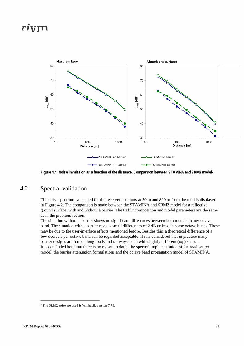
Figure 4.1: Noise immission as a function of the distance. Comparison between STAMINA and SRM2 model2.

4.2 Spectral validation

The noise spectrum calculated for the receiver positions at 50 m and 800 m from the road is displayed in Figure 4.2. The comparison is made between the STAMINA and SRM2 model for a reflective ground surface, with and without a barrier. The traffic composition and model parameters are the same as in the previous section. The situation without a barrier shows no significant differences between both models in any octave band. The situation with a barrier reveals small differences of 2 dB or less, in some octave bands. These may be due to the user-interface effects mentioned before. Besides this, a theoretical difference of a few decibels per octave band can be regarded acceptable, if it is considered that in practice many barrier designs are found along roads and railways, each with slightly different (top) shapes. It is concluded here that there is no reason to doubt the spectral implementation of the road source model, the barrier attenuation formulations and the octave band propagation model of STAMINA.

2 The SRM2 software used is Winhavik version 7.79.


20

30

40

50

60

70

63 125 250 500 1000 2000 4000 8000Frequency [Hz]

LAeq

[dB

]

50m SRM250m STAMINA800m SRM2800m STAMINA

no barrier

10

20

30

40

50

60

63 125 250 500 1000 2000 4000 8000Frequency [Hz]

LAeq

[dB

]

4m barrier

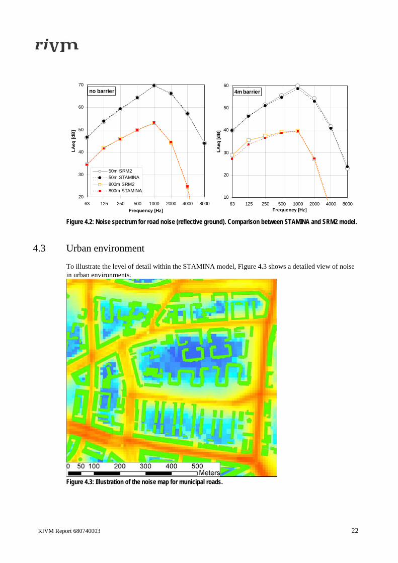
Figure 4.2: Noise spectrum for road noise (reflective ground). Comparison between STAMINA and SRM2 model.

4.3 Urban environment

To illustrate the level of detail within the STAMINA model, Figure 4.3 shows a detailed view of noise in urban environments.

Figure 4.3: Illustration of the noise map for municipal roads.


In Figure 4.3, buildings are added to the noise map for the municipal roads. The grid size close to the source is 10 by 10 m, and the buildings are indicated by the green areas, and it can be seen that large buildings located parallel to the roads can act as noise barriers for the area behind these buildings, and that the noise can propagate alongside buildings located perpendicular to the road.

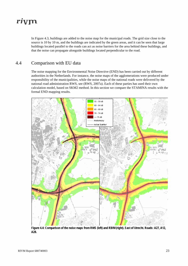
4.4 Comparison with EU data

The noise mapping for the Environmental Noise Directive (END) has been carried out by different authorities in the Netherlands. For instance, the noise maps of the agglomerations were produced under responsibility of the municipalities, while the noise maps of the national roads were delivered by the national road administration RWS, see (RWS, 2007a). Each of these parties has used their own calculation model, based on SKM2 method. In this section we compare the STAMINA results with the formal END mapping results.

Figure 4.4: Comparison of the noise maps from RWS (left) and RIVM (right). East of Utrecht. Roads: A27, A12, A28.


The noise maps for the national roads are compared in Figure 4.4. The left-hand map is the formal result delivered by RWS. This map is created by the Silence model (RWS, 2007b), which is an SKM2 implementation like STAMINA. The only input data that is equal in generating both maps are the traffic data (intensity and speeds) and noise barriers. The ground attenuation and dwelling characteristics may differ between both approaches3. There is generally a good resemblance between both maps. Figure 4.5 gives the number of dwellings exposed to Lden > 65 dB within six agglomerations. The formal END results of each of the agglomerations was produced by different project teams using different mapping software and probably also a different approach towards data collection. Though the traffic flow on the municipal roads in the RIVM approach was a rather coarse estimation, based on road type instead of counts, the overall difference between the RIVM map and the formal ones is not so large.

number of dwe llings > 65 dB road traffic noise

0

20000

40000

60000

80000

100000

120000

Utrecht Amsterdam Den Haag Rotterdam Eindhoven Heerlen

ENDRIVM

Figure 4.5: Comparison of the Environmental Noise Directive Data (END) with the STAMINA (RIVM) model.

3 The motorway exits and connection roads near the junctions are only drawn for clarity in the RWS map, they are not modeled as acoustical sources.


5 Noise maps and applications This chapter shows the noise maps using the models described in the previous chapters. First the noise sources will be treated separately, and a cumulative noise map for all the noise sources in the Netherlands will be shown. Subsequently some applications of these noise maps will be mentioned.

5.1 Noise maps

5.1.1 Roadway traffic Figure 5.1 shows the noise map for the main and secondary motorways in the Netherlands. A detailed view of the mapping of municipal roads was shown in Figure 4.3

Figure 5.1: Noise map of the Netherlands for the main and secondary motorways.


5.1.2 Railway traffic Figure 5.2 shows the noise map of the railway network in the Netherlands. This includes the high speed rail network, which started its service in 2009.

Figure 5.2: Noise map of the railway noise in the Netherlands.


5.1.3 Industrial noise For the noise map of the industrial noise, a more detailed example is shown in Figure 5.3. Here, a noise map of the Rijnmond area is shown, containing the Rotterdam harbour and it is the largest industrial region of the Netherlands. For clarity, residential areas are indicated by the black regions.

Figure 5.3: Noise map of the industrial noise in the Rijnmond area. Although a large region has a noise exposure of over 60 dB, by including the locations of dwellings in this noise map it can be seen that most of the dwellings are located in the regions with a relatively low noise exposure to industrial noise. An example of a quantitative analysis of the noise exposure to dwellings is included in section 5.2.


5.1.4 Cumulative noise map Finally, combining the noise maps for roadway, railway traffic and industrial noise, a cumulative noise map for all noise sources in the Netherlands can be made. This noise map also includes data for air traffic. This data was provided by the Dutch National Aerospace Laboratory, using (NLR, 2007) to determine the equivalent noise levels. For Schiphol airport, a region of interest of 55 x 71 km2 was used.

Figure 5.4: Cumulative noise map of the Netherlands.


5.2 Applications and discussion

5.2.1 Current applications The cumulative noise map from Figure 5.4 can be consulted online4. People interested can use their postal code to obtain information on the noise exposure in their neighborhood. The noise map is also included within the Areas of Environmental Concern project (Du Pon et al., 2008), which aims to provide policy makers, urban planners and local populations with a comprehensive overview of the residential areas urgently needing attention from an environmental standpoint. They can also be used for global assessments of new development plans. Other applications where the STAMINA model has been used are studies performed by RIVM on the influence of hybrid cars on noise exposure (Verheijen et al., 2008), assessment of noise from wind turbines (Verheijen et al., 2009) and the impact of low frequency noise levels in the Netherlands (Schreurs et al., 2008). For example, noise maps can be combined with residential data in a way shown in Figure 5.4, and an analysis of the number of dwellings and inhabitants exposed to a certain type of noise can be performed. Table 5.1 gives an example of such an analysis, in this case for wind turbine noise (Verheijen et al., 2009). Table 5.1 Example of the analysis of noise exposure of wind turbine noise to dwellings. Noise level Number of

dwellings (#) Number of inhabitants (#)

Annoyed people

Highly annoyed people

Above 29 dB 200.000 440.000 4200 1500 Above 40 dB 6810 15.250 1640 760 Above 45 dB 1390 3110 740 400 Above 47 dB 810 1810 540 310 Above 50 dB 330 740 290 180

5.2.2 Uncertainties and future developments Although the noise maps are fairly accurate and follow the Dutch standard calculation methods, it should be noted that uncertainties are present in the noise maps. The main factors for uncertainties are the source data (traffic numbers and sound power levels), which should be updated with the most recent knowledge regularly. For this reason, the noise maps produced with the STAMINA model cannot be used as a validity tool for the Dutch Noise legislation. In the future, RIVM endeavors to update its source data in order to keep the noise maps as accurate as possible. This includes updating the traffic numbers for the main and secondary motorways in the Netherlands, and adding a height parameter for the main motorways, which at many places in the Netherlands are not at ground level. For the municipal roads, data provided by the Dutch cooperation program for air quality can be used for an update of the source data.

4 http://www.rivm.nl/milieuportaal/onderwerpen/geluid/geluidbelasting/


References ASWIN, 2004. Het Akoestisch Spoorboekje, emissieregister spoorgeluid. ProRail, 2004. CROW, 2004. Karteringsvoorschriften wegen railverkeerslawaai, bijlage 3 behorende bij artikel 8 van de regeling omgevingslawaai, http://www.stillerverkeer.nl/index.php?section=rmv&subject=kartering Dassen, T. et al., 2000. Geluid in de vijfde Milieuverkenning Achtergronden (Background report to the fifth Environmental Outlook: Noise ), RIVM report 408129009, Bilthoven. Du Pon, B. et al., 2008. Milieuaandachtsgebieden in Nederland (Areas of Environmental Concern in the Netherlands), RIVM report 680300005, Bilthoven. Kadaster, 2006. TOP 10 Vectorbestand, Topografische dienst Kadaster, http://www.kadaster.nl/zakelijk/producten/topografische_dienst_top10vector.html M+P, 1991. Kentallen stand der techniek industriële inrichtingen, Geluidsconvenant Rijnmond-west, M+P Raadgevend Ingenieurs BV Aalsmeer. MVM 91.5.1 d.d.911017 NLR, 2007. Voorschrift voor de berekening van de Lden en Lnight geluidbelasting in dB(A) ten gevolge van vliegverkeer van en naar de luchthaven Schiphol. NLR-CR-2001-372-PT-1&2. RWS, 2007a. Noise maps of national roads, map number: 17d_tcm174-140851.pdf, http://www.rijkswaterstaat.nl/wegen/plannen_en_projecten/geluid_rond_snelwegen_nederland/geluidskaart/geluidskaarten_dag.aspx RWS, 2007b. For an introduction to the Silence 3 model: http://www.silence.nl/introduction.html Scheeper, P., Poutsma H.J., Rozema, D.J., 1980. Voorschrift voor de berekening van de geluidbelasting door vliegtuigen, NLR report nr. LL-HR-20-01, Amsterdam 1980. Schreurs, E.M., Verheijen E.N.G., Potma, C.J.M., Jabben, J., 2009. Noise Monitor 2008, RIVM Report 680740002, RIVM, Bilthoven. Schreurs, E.M., Koeman, T., Jabben, J., 2008. Low frequency noise impact of road traffic in the Netherlands, proceedings of Acoustics08, Paris. Van den Berg, F., Pedersen E., Bouma, J., Bakker, R., 2008 WINDFARMperception: Visual and acoustic impact of wind turbine of wind turbine farms on residents Report FP6-2005-Science-and-Society-20. University of Groningen, Göteborg University. Verheijen, E. et al., 2008. Invloed hybride voertuigen op de geluidbelasting, RIVM letter report 680300006, Bilthoven. Verheijen, E. et al., 2009. Evaluatie nieuwe normstelling windturbinegeluid (Assessment of new limit values for wind turbines), RIVM report 680300007, Bilthoven, 2009. VROM, 1997. Ministry of Housing, Spatial Planning and the Environment, Naar een landelijk beeld van de verstoring, publikatiereeks verstoring, nr. 12/1997.


VROM, 2006a. Ministry of Housing, Spatial Planning and the Environment, Appendix III to chapter 3 on Road Noise of the Reken- en meetvoorschrift geluidhinder 2006. VROM, 2006b. Ministry of Housing, Spatial Planning and the Environment, Appendix IV to chapter 4 on Railway Noise of the Reken- en meetvoorschrift geluidhinder 2006. VROM, 2006c. Ministry of Housing, Spatial Planning and the Environment, Module C2 on Industrial Noise of the Reken- en meetvoorschrift geluidhinder 2006 WGAEN, 2007. Good Practice Guide for Strategic Noise Mapping and the Production of Associated Data on Noise Exposure, European Commission Working Group Assessment of Environmental Noise, Second position paper, January 2006. http://ec.europa.eu/environment/noise/mapping.htm


Appendix A: Examples of Ascii input data used by STAMINA Table A1.1 Example of input data for motorways. nr xstart ystart xend yend hsl tsl hsr tsr road ld le ln md me mn hd he hn vl vm vh dE hr 0 53233.2 370327 53469.3 370247 0 0 0 0 0 0 0 0 0 0 0 0 0 0 80 80 80 0 0 1 53469.3 370247 53641.2 370237 0 0 0 0 0 0 0 0 0 0 0 0 0 0 80 80 80 0 0 2 53014 408395 53028.9 408386 0 0 0 0 0 1380 111.2 71.8 803.8 29 22.2 217.2 20.6 22.2 70 70 70 0 0 3 53028.9 408386 53201 408271 0 0 0 0 0 0 0 0 0 0 0 0 0 0 70 70 70 0 0 4 53264.3 408267 53289.4 408270 0 0 0 0 0 0 0 0 0 0 0 0 0 0 100 80 80 0 0 5 53264.3 408267 53289.4 408270 0 0 0 0 0 0 0 0 0 0 0 0 0 0 70 70 70 0 0 6 53201 408271 53264.3 408267 0 0 0 0 0 0 0 0 0 0 0 0 0 0 70 70 70 0 0 7 53289.4 408270 53408 408285 0 0 0 0 0 0 0 0 0 0 0 0 0 0 70 70 70 0 0 8 53641.2 370237 53890.8 370223 0 0 0 0 0 932.8 63.6 31.8 428.2 17 6.4 120.8 6.4 8.4 80 80 80 0 0 9 53890.8 370223 54140.5 370211 0 0 0 0 0 932.8 63.6 31.8 428.2 17 6.4 120.8 6.4 8.4 80 80 80 0 0

10 …. … Nr: number of road segment. The database consists of approximately 28000 segments. Each segment no larger than 250 m Xstart horizontal RD coordinate of the beginning of the segment Hsl: height of barrier left from the segment Tsl: type of barrier 1 = normal barrier, 2 = earth wall Road: type of road segment, 0 = dense asphaltic concrete, 1 = single porous layer porous, 2 = double porous layer Ld/e/n: number of light vehicles per hour in the day/evening/night time period 7:00-19:00/19:00-23:00/23:00-7:00 h Md/e/n: number of middle weight trucks per hour in the day/evening/night time period 7:00-19:00/19:00-23:00/23:00-7:00 h Hd/e/n: number of heavy weight trucks per hour in the day/evening/night time period 7:00-19:00/19:00-23:00/23:00-7:00 h Vl/m/h: average speed of light/middle weight/heavy vehicles km/h dE optional correction of noise emission, 0 by default


Table A1.2 Example of input data for municipal roads.

nr xbegin Ybegin Xend Yend volume correction Fobj_left Fobj_Rright 1 249959 607306 249985 607300 6621 0 0.019802 0.019802 2 249985 607300 249993 607298 6621 0 0.019802 0.019802 3 249993 607298 250000 607296 6621 0 0.058923 0.019802 4 250000 607296 250019 607280 6621 0 0.019802 0.019802 5 250028 607286 250042 607269 6621 0 0.019802 0.019802 6 250019 607280 250028 607286 6621 0 0.019802 0.019802 6 250019 607280 250053 607248 6621 2 0.019802 0.019802 7 249951 607271 249959 607306 6621 0 0.019802 0.019802 8 250042 607269 250050 607261 6621 1 0.019802 0.019802 9 250050 607261 250058 607258 6621 1 0.019802 0.019802

10 250058 607258 250069 607255 6621 0 0.019802 0.019802 Nr : number of road segment. The database consists of approximately 600,000 segments. Each segment no larger than 100 m Xbegin : as for motorways Volume : estimated number of vehicles passing by in 24 hour. The traffic composition over different vehicle categories is estimated according to (Dassen et al., 2000) Fobj_left: object fraction of dwellings located left of the segment, increasing noise emission towards the right Fobj_right: object fraction of dwellings locater right of the segment, increasing noise emission towards the left Fobj left and right were determined for each road segment by using Top 10 data of all dwellings in the Netherlands


Table A1.3 Example of input data for railways.

nr Xstart Ystart Xend Yend hsl asl tsl hsr asr tsr Eday Eev Enight d 1 91711 443163 91846 443395 0 0 0 0 0 0 85 85 80 0 2 91846 443395 91981 443627 0 0 0 0 0 0 85 85 80 0 3 91981 443627 92116 443859 0 0 0 0 0 0 85 85 80 0 4 92116 443859 92251 444091 0 0 0 0 0 0 85 85 80 0 5 92251 444091 92403.2 444288 0 0 0 0 0 0 85 85 80 0 6 92403.2 444288 92555.3 444486 0 0 0 0 0 0 85 85 80 0 7 92555.3 444486 92707.5 444683 0 0 0 0 0 0 85 85 80 0 8 92707.5 444683 92859.7 444880 0 0 0 0 0 0 85 85 80 0 9 92859.7 444880 93011.8 445078 0 0 0 0 0 0 85 85 80 0

10 93011.8 445078 93164 445275 0 0 0 0 0 0 85 85 80 0 Nr: number of track segment. The database consists of approximately 63000 track segments. Each segment no larger than 250 m Xstart horizontal RD coordinate of the beginning of the segment Hsl: height of barrier left from the segment Asl: distance of barrier to the centre of the nearest track Tsl: type of barrier 1 = normal barrier, 2 = earth wall Eday/ev/night: Emission numbers according to (Aswin, 2004) dE optional correction of noise emission, 0 by default


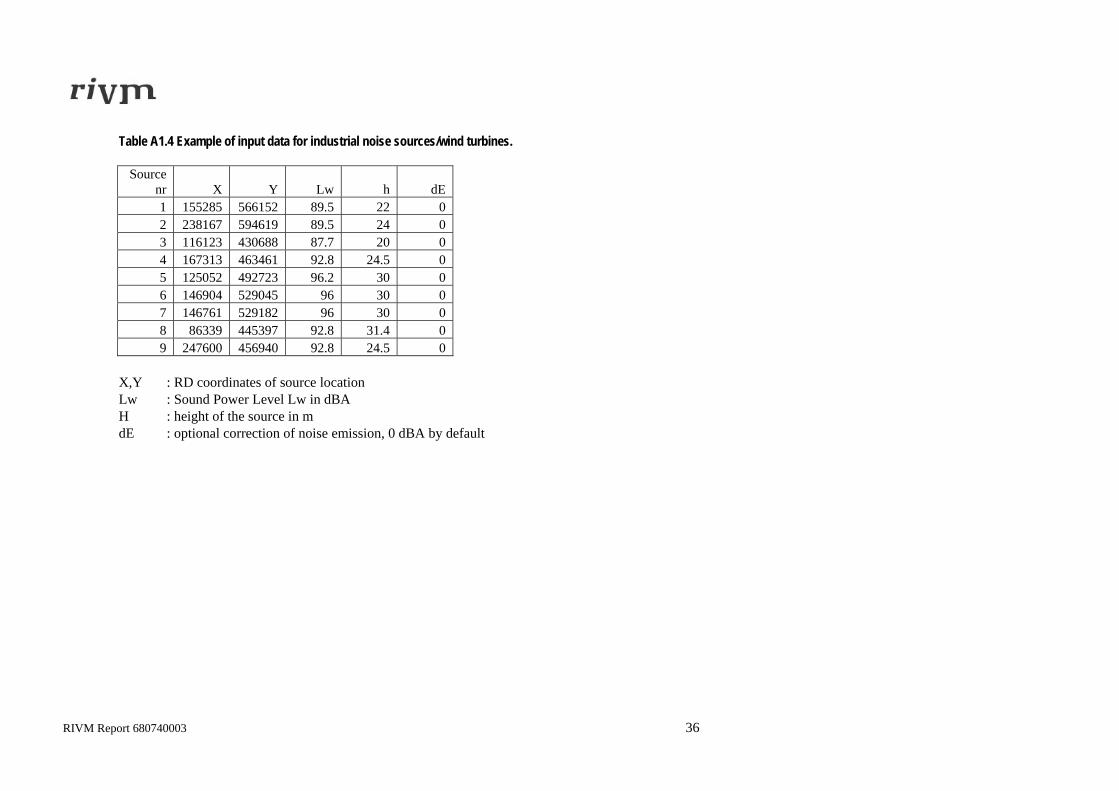
Table A1.4 Example of input data for industrial noise sources/wind turbines.

Source nr X Y Lw h dE 1 155285 566152 89.5 22 0 2 238167 594619 89.5 24 0 3 116123 430688 87.7 20 0 4 167313 463461 92.8 24.5 0 5 125052 492723 96.2 30 0 6 146904 529045 96 30 0 7 146761 529182 96 30 0 8 86339 445397 92.8 31.4 0 9 247600 456940 92.8 24.5 0

X,Y : RD coordinates of source location Lw : Sound Power Level Lw in dBA H : height of the source in m dE : optional correction of noise emission, 0 dBA by default


RIVM

National Institute

for Public Health

and the Environment

P.O. Box 1

3720 BA Bilthoven

The Netherlands

www.rivm.com

RIVM

National Institutefor Public Healthand the Environment

P.O. Box 13720 BA BilthovenThe Netherlandswww.rivm.nl

RIVM rapport 680740003 STAMINA-Model description · STAMINA-Model description ... within the...

Documents

Transcript of RIVM rapport 680740003 STAMINA-Model description · STAMINA-Model description ... within the...