
Riten Gupta - Electrical Engineering and Computer...
164
Transcript of Riten Gupta - Electrical Engineering and Computer...

QUANTIZATION STRATEGIES FOR LOW-POWER
COMMUNICATIONS
by
Riten Gupta
A dissertation submitted in partial ful�llmentof the requirements for the degree of
Doctor of Philosophy(Electrical Engineering: Systems)in The University of Michigan
2001
Doctoral Committee:Professor Alfred O. Hero, III, ChairProfessor Robert W. KeenerProfessor David L. Neuho�Associate Professor Marios C. PapaefthymiouProfessor Wayne E. Stark
ABSTRACT
QUANTIZATION STRATEGIES FOR LOW-POWER COMMUNICATIONS
by
Riten Gupta
Chair: Alfred O. Hero, III
Power reduction in digital communication systems can be achieved in many ways. Re-
duction of the wordlengths used to represent data and control variables in the digital circuits
comprising a communication system is an e�ective strategy, as register power consumption
increases with wordlength. Another strategy is the reduction of the required data trans-
mission rate, and hence speed of the digital circuits, by eÆcient source encoding. In this
dissertation, applications of both of these power reduction strategies are investigated.
The LMS adaptive �lter, for which a myriad of applications exists in digital communi-
cation systems, is optimized for performance with a power consumption constraint. This
optimization is achieved by an analysis of the e�ects of wordlength reduction on both perfor-
mance { transient and steady-state { as well as power consumption. Analytical formulas for
the residual steady-state mean square error (MSE) due to quantization versus wordlength
of data and coeÆcient registers are used to determine the optimal allocation of bits to data
versus coeÆcients under a power constraint. A condition on the wordlengths is derived
under which the potentially hazardous transient \slowdown" phenomenon is avoided. The
algorithm is then optimized for no slowdown and minimum MSE. Numerical studies are
presented for the case of LMS channel equalization.

Next, source encoding by vector quantization is studied for distributed hypothesis test-
ing environments with simple binary hypotheses. It is shown that, in some cases, low-rate
quantizers exist that cause no degradation in hypothesis testing performance. These cases
are, however, uncommon. For the majority of cases, in which quantization necessarily
degrades performance, optimal many-cell vector quantizers are derived that minimize the
performance loss. These quantizers are optimized using objective functions based on the
Kullback-Leibler statistical divergence, or discrimination, and large deviations theory. Moti-
vated by Stein's lemma, the loss in discrimination between two sources due to quantization
is minimized. Next, formulas for the losses in discrimination between the hypothesized
sources and the so-called \tilted" source are determined. These formulas are used to design
quantizers that maximize the area under an analog to the receiver operating characteristic
(ROC) curve. The optimal quantizer is shown to have �ne resolution in areas where the
log-likelihood ratio gradient is large in magnitude. The techniques are extended to the
design of quantizers optimal for mixed detection-estimation objectives.

c Riten Gupta 2001All Rights Reserved

To my parents and my brother
ii

ACKNOWLEDGEMENTS
I wish to express my sincere gratitude to my dissertation advisor, Professor Alfred Hero.
His guidance and encouragement throughout my graduate career have been invaluable and
unsparing. I would also like to thank Professors Wayne Stark and David Neuho� for their
numerous helpful discussions concerning my research, and their service on my dissertation
committee. Additionally, I am indebted to committee members Professor Robert Keener
and Professor Marios Papaefthymiou for their careful reading and evaluation of this disser-
tation.
I would like to thank my parents for their neverending love and, from the bottom of my
heart, I wish to thank my brother, whose a�ection has always been unequivocal. I owe an
incalculable debt of gratitude to him and to my sister for their unfailing support. Without
you, this dissertation would never have been possible.
Thanks, too, are in order for my friends in California.
Finally, I would like to acknowledge and thank the Army Research OÆce for its gener-
ous �nancial support (Grant ARO DAAH04-96-1-0337) during the course of my graduate
studies.
iii

TABLE OF CONTENTS
DEDICATION . . . . . . . . . . . . . . . . . . . . . . . . . . . . . . . . . . . . . . ii
ACKNOWLEDGEMENTS . . . . . . . . . . . . . . . . . . . . . . . . . . . . . . iii
LIST OF TABLES . . . . . . . . . . . . . . . . . . . . . . . . . . . . . . . . . . . vi
LIST OF FIGURES . . . . . . . . . . . . . . . . . . . . . . . . . . . . . . . . . . vii
LIST OF APPENDICES . . . . . . . . . . . . . . . . . . . . . . . . . . . . . . . xi
CHAPTERS
1 Introduction . . . . . . . . . . . . . . . . . . . . . . . . . . . . . . . . . . . 11.1 Overview of Dissertation . . . . . . . . . . . . . . . . . . . . . . . . 11.2 Register Length and Power . . . . . . . . . . . . . . . . . . . . . . . 21.3 Components of a Digital Communication System . . . . . . . . . . 31.4 Lossless Source Coding and Quantization . . . . . . . . . . . . . . . 51.5 Power Reduction by Quantization . . . . . . . . . . . . . . . . . . . 6
1.5.1 A Simple Power Formula . . . . . . . . . . . . . . . . . . . . 71.5.2 Wordlength Reduction . . . . . . . . . . . . . . . . . . . . . 81.5.3 Source Encoding . . . . . . . . . . . . . . . . . . . . . . . . 9
2 Low-Power LMS Adaptation . . . . . . . . . . . . . . . . . . . . . . . . . . 102.1 Introduction . . . . . . . . . . . . . . . . . . . . . . . . . . . . . . . 10
2.1.1 The LMS Algorithm . . . . . . . . . . . . . . . . . . . . . . 112.1.2 Overview of Previous Work . . . . . . . . . . . . . . . . . . 122.1.3 Overview of Contribution . . . . . . . . . . . . . . . . . . . 13
2.2 Finite-Precision LMS Adaptation . . . . . . . . . . . . . . . . . . . 142.2.1 In�nite-Precision LMS Algorithm . . . . . . . . . . . . . . . 142.2.2 Finite-Precision LMS Algorithm . . . . . . . . . . . . . . . . 152.2.3 Power Consumption of LMS Algorithm . . . . . . . . . . . . 162.2.4 Statistical Performance of Finite-Precision LMS Algorithm . 17
2.3 Optimal Bit Allocation Strategies . . . . . . . . . . . . . . . . . . . 242.3.1 Total Bit Budget Constraint . . . . . . . . . . . . . . . . . . 242.3.2 Total Power Budget Constraint . . . . . . . . . . . . . . . . 25
2.4 Numerical Example . . . . . . . . . . . . . . . . . . . . . . . . . . . 252.5 Conclusion . . . . . . . . . . . . . . . . . . . . . . . . . . . . . . . . 31
iv

3 Vector Quantization for Distributed Hypothesis Testing . . . . . . . . . . . 333.1 Introduction . . . . . . . . . . . . . . . . . . . . . . . . . . . . . . . 33
3.1.1 Distributed Hypothesis Testing . . . . . . . . . . . . . . . . 343.1.2 Vector Quantization . . . . . . . . . . . . . . . . . . . . . . 353.1.3 Overview of Previous Work . . . . . . . . . . . . . . . . . . 353.1.4 Overview of Contribution . . . . . . . . . . . . . . . . . . . 37
3.2 Preliminaries . . . . . . . . . . . . . . . . . . . . . . . . . . . . . . 383.2.1 Hypothesis Testing . . . . . . . . . . . . . . . . . . . . . . . 383.2.2 Vector Quantization . . . . . . . . . . . . . . . . . . . . . . 45
3.3 Lossless Quantizers for Distributed Hypothesis Testing . . . . . . . 493.3.1 SuÆcient Quantizers . . . . . . . . . . . . . . . . . . . . . . 533.3.2 Neyman-Pearson Quantizers . . . . . . . . . . . . . . . . . . 563.3.3 Examples of Lossless Quantizers . . . . . . . . . . . . . . . . 583.3.4 Estimation Performance of Lossless Quantizers . . . . . . . 61
3.4 Lossy Quantizers for Distributed Hypothesis Testing . . . . . . . . 613.4.1 Sequences of Quantizers . . . . . . . . . . . . . . . . . . . . 623.4.2 Log-Likelihood Ratio Quantizers . . . . . . . . . . . . . . . 623.4.3 Estimation-Optimal Quantizers . . . . . . . . . . . . . . . . 643.4.4 Small-Cell Quantizers . . . . . . . . . . . . . . . . . . . . . . 65
3.5 Asymptotic Analysis of Quantization for Hypothesis Testing . . . . 653.5.1 Asymptotic Discrimination Losses . . . . . . . . . . . . . . . 663.5.2 Fisher Covariation Pro�le . . . . . . . . . . . . . . . . . . . 683.5.3 Discriminability . . . . . . . . . . . . . . . . . . . . . . . . . 693.5.4 Comparison to Bennet's Integral . . . . . . . . . . . . . . . 71
3.6 Optimal Small-Cell Quantizers for Hypothesis Testing . . . . . . . 713.6.1 Maximum Discrimination . . . . . . . . . . . . . . . . . . . 713.6.2 Maximum Power . . . . . . . . . . . . . . . . . . . . . . . . 743.6.3 Maximum Area under ROC Curve . . . . . . . . . . . . . . 763.6.4 Optimal Log-Likelihood Ratio Quantizers . . . . . . . . . . 803.6.5 Mixed Objective Function . . . . . . . . . . . . . . . . . . . 80
3.7 Numerical Examples . . . . . . . . . . . . . . . . . . . . . . . . . . 823.7.1 Scalar Gaussian Sources . . . . . . . . . . . . . . . . . . . . 823.7.2 Two-Dimensional Uncorrelated Gaussian Sources . . . . . . 903.7.3 Two-Dimensional Correlated Gaussian Sources . . . . . . . 963.7.4 Triangular Sources . . . . . . . . . . . . . . . . . . . . . . . 1023.7.5 Piecewise-Constant Sources . . . . . . . . . . . . . . . . . . 1073.7.6 Two-Dimensional Image Sources . . . . . . . . . . . . . . . 109
3.8 Conclusion . . . . . . . . . . . . . . . . . . . . . . . . . . . . . . . . 111
APPENDICES . . . . . . . . . . . . . . . . . . . . . . . . . . . . . . . . . . . . . . 113
BIBLIOGRAPHY . . . . . . . . . . . . . . . . . . . . . . . . . . . . . . . . . . . . 145
v

LIST OF TABLES
Table
2.1 Percent di�erence between theoretical and measured slowdown points for�nite-precision LMS channel equalizer with �2s = 0:06, �2n = 10�8, � = 1=4,IIR channel with single pole at a1, and � = 10�3. . . . . . . . . . . . . . . . 26
3.1 Reconstruction MSE of 64-cell estimation-optimal quantizer, ROC-optimalcongruent cell-quantizer, and ROC-optimal LLR quantizer for two-dimensional uncorrelated Gaussian example. . . . . . . . . . . . . . . . . . . 96
3.2 Areas under L1(L0) curves without quantization and with quantization forone-dimensional triangular example. AL = area with no quantization, Ao
L
= area after quantization with ROC-optimal quantizer, A�L = area after
quantization with quantizer using point density ��. . . . . . . . . . . . . . . 104
3.3 Di�erence in ROC curve areas for one-dimensional triangular example.�AROC = Ao
ROC �A�ROC where Ao
ROC = area under ROC curve after quan-tization with ROC-optimal quantizer and A�
ROC = area under ROC curveafter quantization with quantizer using point density ��. . . . . . . . . . . . 105
vi

LIST OF FIGURES
Figure
1.1 Power versus bit width B as function of AR parameter a1 for loading a B-bitregister with successive samples of an AR(1) process. Curves are normalizedrelative to power P16 consumed for a white sequence in a 16-bit register. Inthe plot, the bit width is reduced from right to left by eliminating LSB's. . 4
1.2 Digital communication system. . . . . . . . . . . . . . . . . . . . . . . . . . 4
2.1 In�nite-precision LMS algorithm. . . . . . . . . . . . . . . . . . . . . . . . . 14
2.2 Finite-precision LMS algorithm. . . . . . . . . . . . . . . . . . . . . . . . . . 15
2.3 Surface plot of excess MSE due to �nite precision as a function of Bd and Bc
for single-pole IIR channel. . . . . . . . . . . . . . . . . . . . . . . . . . . . 21
2.4 Contour plot of excess MSE due to �nite precision as a function of Bd andBc for single-pole IIR channel. . . . . . . . . . . . . . . . . . . . . . . . . . 21
2.5 Example of slowdown. . . . . . . . . . . . . . . . . . . . . . . . . . . . . . . 23
2.6 Learning curves of LMS �lters equalizing IIR channel with Gaussian inputwithout slowdown. . . . . . . . . . . . . . . . . . . . . . . . . . . . . . . . . 27
2.7 IIR channel with Gaussian input: data bit allocation factors under BT con-straint as functions of BT . . . . . . . . . . . . . . . . . . . . . . . . . . . . . 28
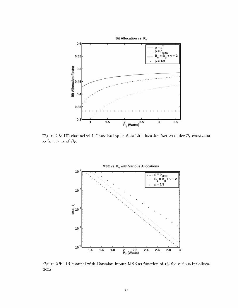
2.8 IIR channel with Gaussian input: data bit allocation factors under PT con-straint as functions of PT . . . . . . . . . . . . . . . . . . . . . . . . . . . . . 29
2.9 IIR channel with Gaussian input: MSE as function of PT for various bitallocations. . . . . . . . . . . . . . . . . . . . . . . . . . . . . . . . . . . . . 29
2.10 32-tap LMS channel equalizer: data bit allocation factors under BT con-straint as functions of BT . . . . . . . . . . . . . . . . . . . . . . . . . . . . . 30
2.11 32-tap LMS channel equalizer: data bit allocation factors under PT constraintas functions of PT . . . . . . . . . . . . . . . . . . . . . . . . . . . . . . . . . 30
vii
2.12 32-tap LMS channel equalizer: MSE as function of PT for various bit alloca-tions. . . . . . . . . . . . . . . . . . . . . . . . . . . . . . . . . . . . . . . . . 31
3.1 Sensor network. . . . . . . . . . . . . . . . . . . . . . . . . . . . . . . . . . . 34
3.2 ROC curves of Neyman-Pearson tests with quantized and unquantized datafor n = 1 and n = 2 observations. For n = 1, the quantizer is a Neyman-Pearson quantizer for several thresholds. . . . . . . . . . . . . . . . . . . . . 59
3.3 Border (dashed line) between Neyman-Pearson regions for Gaussian sourcesand cells of a two-dimensional product quantizer (solid lines). . . . . . . . . 60
3.4 A log-likelihood ratio quantizer. . . . . . . . . . . . . . . . . . . . . . . . . . 62
3.5 Log-likelihood ratio quantizer for two-dimensional Gaussian sources withidentity covariance matrices. . . . . . . . . . . . . . . . . . . . . . . . . . . . 64
3.6 Contours of log-likelihood ratio �(x) (dashed lines) and some cells of anoptimal ellipsoidal-cell quantizer. . . . . . . . . . . . . . . . . . . . . . . . . 74
3.7 Example of L1(L0) and L1(L0). . . . . . . . . . . . . . . . . . . . . . . . . . 77
3.8 Source densities and �(x) for one-dimensional Gaussian example. . . . . . . 83
3.9 ROC-optimal, discrimination-optimal, and estimation-optimal point densi-ties for one-dimensional Gaussian example. . . . . . . . . . . . . . . . . . . 84
3.10 L1(L0) curves without quantization and with quantization by ROC-optimal,discrimination-optimal, and estimation-optimal quantizers with N = 8 cellsfor one-dimensional Gaussian example. ROC-optimal quantizer has best per-formance, on average, while detection-optimal quantizer yields largest valueof L(�q0k�q1). . . . . . . . . . . . . . . . . . . . . . . . . . . . . . . . . . . . . 85
3.11 ROC curves with n = 2 observations and data quantized by ROC-optimal,discrimination-optimal, and estimation-optimal quantizers with N = 16 cellsfor one-dimensional Gaussian example. . . . . . . . . . . . . . . . . . . . . . 86
3.12 Reconstruction MSE with ROC-optimal, discrimination-optimal, andestimation-optimal quantizers with N = 16 cells for one-dimensional Gaus-sian example. . . . . . . . . . . . . . . . . . . . . . . . . . . . . . . . . . . . 86
3.13 Optimal point densities for ROC area and Cherno� information for one-dimensional Gaussian sources with �0 = 0 and �1 = 8. . . . . . . . . . . . . 89
3.14 L1(L0) curves without quantization and with quantization by ROC-optimaland Cherno�-information-optimal quantizers for one-dimensional Gaussiansources with N = 8, �0 = 0, and �1 = 8. . . . . . . . . . . . . . . . . . . . . 89
3.15 Source densities for two-dimensional uncorrelated Gaussian example. . . . . 90
viii

3.16 Two-dimensional uncorrelated Gaussian example: (a) �(x), (b) log-likelihoodratio �(x), (c) discriminability kr�(x)k2, (d) ROC-optimal point density,(e) discrimination-optimal point density, (f) estimation-optimal pointdensity. . . . . . . . . . . . . . . . . . . . . . . . . . . . . . . . . . . . . . . 91
3.17 ROC-optimal 64-cell vector quantizer for two-dimensional uncorrelated Gaus-sian example. . . . . . . . . . . . . . . . . . . . . . . . . . . . . . . . . . . . 92
3.18 Discrimination-optimal 64-cell vector quantizer for two-dimensional uncorre-lated Gaussian example. . . . . . . . . . . . . . . . . . . . . . . . . . . . . . 93
3.19 Estimation-optimal 64-cell vector quantizer for two-dimensional uncorrelatedGaussian example. . . . . . . . . . . . . . . . . . . . . . . . . . . . . . . . . 93
3.20 L1(L0) curves without quantization and with quantization by ROC-optimal,discrimination-optimal, and estimation-optimal quantizers with N = 64 cellsfor two-dimensional uncorrelated Gaussian example. ROC-optimal quantizerhas best performance, on average, while detection-optimal quantizer yieldslargest value of L(�q0k�q1). . . . . . . . . . . . . . . . . . . . . . . . . . . . . . 94
3.21 Optimal 64-cell log-likelihood ratio quantizer for two-dimensional uncorre-lated Gaussian example. . . . . . . . . . . . . . . . . . . . . . . . . . . . . . 95
3.22 L1(L0) curves with 64-cell ROC-optimal congruent-cell quantizer and 64-cell ROC-optimal LLR quantizer for two-dimensional uncorrelated Gaussianexample. . . . . . . . . . . . . . . . . . . . . . . . . . . . . . . . . . . . . . . 95
3.23 Optimal 64-cell vector quantizer with mixed objective function with � = 1=2for two-dimensional uncorrelated Gaussian example. . . . . . . . . . . . . . 97
3.24 Detection and estimation performance of optimal 64-cell vector quantizerwith mixed objective function for two-dimensional uncorrelated Gaussianexample. . . . . . . . . . . . . . . . . . . . . . . . . . . . . . . . . . . . . . . 97
3.25 Source densities for two-dimensional correlated Gaussian example. . . . . . 98
3.26 Two-dimensional correlated Gaussian example: (a) �(x), (b) log-likelihoodratio �(x), (c) discriminability kr�(x)k2, (d) ROC-optimal point density,(e) discrimination-optimal point density, (f) estimation-optimal pointdensity. . . . . . . . . . . . . . . . . . . . . . . . . . . . . . . . . . . . . . . 99
3.27 ROC-optimal 64-cell vector quantizer for two-dimensional correlated Gaus-sian example. . . . . . . . . . . . . . . . . . . . . . . . . . . . . . . . . . . . 100
3.28 Discrimination-optimal 64-cell vector quantizer for two-dimensional corre-lated Gaussian example. . . . . . . . . . . . . . . . . . . . . . . . . . . . . . 100
3.29 Estimation-optimal 64-cell vector quantizer for two-dimensional correlatedGaussian example. . . . . . . . . . . . . . . . . . . . . . . . . . . . . . . . . 101
ix

3.30 L1(L0) curves without quantization and with quantization by ROC-optimal,discrimination-optimal, and estimation-optimal quantizers with N = 64 cellsfor two-dimensional correlated Gaussian example. ROC-optimal quantizerhas best performance, on average, while detection-optimal quantizer yieldslargest value of L(�q0k�q1). . . . . . . . . . . . . . . . . . . . . . . . . . . . . . 101
3.31 Triangular source example: (a) source densities, (b) �(x), (c) gradient (deriva-tive) of log-likelihood ratio, (d) ROC-optimal point density. . . . . . . . . . 103
3.32 L1(L0) curves for one-dimensional triangular example without quantizationand with quantization using point densities �o and ��, with N = 8 cells. . . 106
3.33 Log-likelihood ratio for one-dimensional triangular example. . . . . . . . . . 106
3.34 Piecewise-constant source example: (a) source densities, (b) �(x), (c) gradi-ent (derivative) of log-likelihood ratio, (d) ROC-optimal point density. . . . 108
3.35 Null density for two-dimensional image example. . . . . . . . . . . . . . . . 109
3.36 Alternate density for two-dimensional image example. . . . . . . . . . . . . 110
3.37 ROC-optimal point density for two-dimensional image example. . . . . . . . 110
A.1 Uniform scalar quantizer. . . . . . . . . . . . . . . . . . . . . . . . . . . . . 114
A.2 Regions de�ned in equation (A.3). . . . . . . . . . . . . . . . . . . . . . . . 115
B.1 PT versus BT for di�erent power relations with �a � 1:4 mW and �t � 6:8mW. . . . . . . . . . . . . . . . . . . . . . . . . . . . . . . . . . . . . . . . . 120
x

LIST OF APPENDICES
APPENDIX
A Derivation of Bound on Register Power Consumption . . . . . . . . . . . . . 114
B Iteration Power of LMS Algorithm . . . . . . . . . . . . . . . . . . . . . . . 118
C Derivation of Mean Convergence Rate, Weight-Error Covariance, and ExcessMean Square Error . . . . . . . . . . . . . . . . . . . . . . . . . . . . . . . . 121
D Derivation of Optimal Bit Allocation Factors . . . . . . . . . . . . . . . . . 126
E Derivation of Asymptotic Discrimination Losses . . . . . . . . . . . . . . . . 128
F Procedure for Generating Vector Quantizers . . . . . . . . . . . . . . . . . . 142
xi

CHAPTER 1
Introduction
1.1 Overview of Dissertation
Communication systems engineers have for decades tackled problems inherent to the de-
sign of eÆcient and reliable systems. Key objectives have been: low bandwidth utilization,
low transmitter power, and high data throughput, all while achieving a reliable commu-
nication link [59]. Advances in high-speed electronic devices and circuits have enabled
communications engineers to realize signi�cant progress toward these goals. This progress
has been the impetus for the burgeoning wireless industry. Overlooked in the design process
has been an analysis of the relation of system performance to the power consumption of
the digital circuits that comprise the transceiver [16]. Lacking such an analytical power-
performance relationship, designers have resorted to trial-and-error methods in e�orts to
minimize power consumption. The intent of this dissertation is to develop the aforemen-
tioned power-performance relationship as well as procedures that utilize the relationship for
communication system design.
Any component of a digital communication system comprised of electronic circuitry {
digital or analog { is a power-consuming device. The most obvious strategy for power
reduction in the digital circuitry is the reduction of the wordlengths used to represent in-
ternal variables [52]. This dissertation will focus on the wordlength reduction approach to
power minimization. It is well known that power consumption of digital circuits increases
with the wordlength. Wordlength reduction, however, generally entails a degradation in
1

performance of the communication system. It is bene�cial, therefore, to understand, quan-
titatively, the e�ect of wordlength reduction on system performance. Equally important
is the development of procedures to compress data so that it may be stored in reduced-
wordlength registers without signi�cant performance degradation. Both of these issues will
be investigated in this dissertation.
1.2 Register Length and Power
The importance of wordlength reduction can be illustrated by a simple upper bound on
the power consumption of a B-bit register. It is well known that the power consumed by the
operation of loading successive time samples of a random real-valued sequence into a binary
B-bit register is proportional to the average number of bit ips per unit time in the register
[63]. While for a uniform white sequence the average number of bit ips is B=2, in general
this average can be much less than B=2 for a correlated sequence. The reduced activity
can be explained by noting that for correlated sequences most signi�cant bits (MSB's) have
lower probability of transitioning than least signi�cant bits (LSB's). Several models for
the power consumption of register loading have been proposed [63]. The following formula,
derived in Appendix A, is an approximate upper bound on the power consumption of a
�xed-point, B-bit register into which is loaded a zero-mean, wide-sense stationary Gaussian
random sequence:
PB � B� ��1� 1
2erf
�h2Bp2R(0) � 2R(1)
i�1��
= Pmax (1.1)
where � is the power dissipation per bit, which depends on factors such as switching load
capacitance and supply voltage, and R(�) is the autocorrelation function of the random
sequence.
A plot of Pmax versus B is given in Figure 1.1 for an AR(1) sequence with real pole
located at a1. For ja1j < 0:9, the power dissipation increases almost linearly as a function
2

of B. Note from Figure 1.1 that for more highly correlated sequences stored in registers
with few bits, the power increase due to increasing bit width (wordlength) is less severe.
This is due to the fact that only the LSB's ip with high probability in two successive
samples of a highly correlated sequence, while for an uncorrelated uniform sequence, all
bits have equal probability (0.5) of ipping. Note also that as the bit width becomes large,
all sequences consume approximately the same power. This is attributable to the fact
that as the wordlength becomes very large, each new register bit is less signi�cant than all
previous bits. Thus, for large wordlengths, a relatively small fraction of the total bits are
signi�cant and, although the sequence may be highly correlated, most of the register bits
are insigni�cant and have probability of ipping equal to approximately one half.
Figure 1.1 provides ample support for the wordlength reduction strategy for low power
design. Even for extremely correlated sequences { which, though they are not common-
place, do arise in digital communications { signi�cant power savings may be achieved by
wordlength reduction according to the bound (1.1). Thus, it is greatly bene�cial to under-
stand the complex relationship between wordlength and performance of digital communi-
cation systems. Furthermore, an investigation of optimal data compression techniques that
may reduce the wordlength required to store data is warranted.
1.3 Components of a Digital Communication System
Figure 1.2 shows the components of a typical digital communication system. The mes-
sage that is to be transmitted is �rst compressed by the source encoder so that it may
be transmitted in an eÆcient manner. Next, the channel encoder adds redundant bits to
the source-encoded data stream in an e�ort to protect the message from errors introduced
by the channel. Finally, the modulator formats the data in a manner that is suitable for
transmission across the physical channel.
At the receiver, the signal coming out of the channel is �rst demodulated. Next, the
channel equalizer attempts to combat distortion arising from possible frequency-selective
3

2 4 6 8 10 12 14 160
0.1
0.2
0.3
0.4
0.5
0.6
0.7
0.8
0.9
1
Bit Width
Pow
er (
norm
aliz
ed)
Power vs. Resolution for AR(1) Process
a1 = 0.000000
a1 = 0.800000
a1 = 0.990000
a1 = 0.999900
a1 = 0.999999
Figure 1.1: Power versus bit width B as function of AR parameter a1 for loading a B-bitregister with successive samples of an AR(1) process. Curves are normalized relative topower P16 consumed for a white sequence in a 16-bit register. In the plot, the bit width isreduced from right to left by eliminating LSB's.
Transmitter
- SourceEncoder
- ChannelEncoder
-Modulator - Channel -
Receiver
- Demodulator - ChannelEqualizer
- ChannelDecoder
- SourceDecoder
-
Figure 1.2: Digital communication system.
4

fading in the channel. The channel decoder then decodes the data stream in an attempt
to faithfully reproduce the source-encoded message. Finally, the source decoder inverts the
operation of the source encoder.
1.4 Lossless Source Coding and Quantization
Besides the transmitted source in Figure 1.2, virtually all signals in a digital communi-
cation system are source coded. These include the input signals to each digital subsystem,
as well as the internal variables of these subsystems.
A source encoder takes an input signal, or source, and represents it in a form that
requires fewer bits than the original representation. The function of the source decoder is
to \reconstruct" the source. The average number of bits needed to represent one source
sample is called the rate of the source encoder. A good source encoder has as low a rate as
possible. Another performance measure of a source encoder is its distortion. The distortion
is a measure of the di�erence between the source and reconstruction. Low distortion is
always desirable. Some signals, such as the internal variables of a channel equalizer, are
encoded, but { as their reconstructions are not required { never decoded.
Source encoders can be characterized as lossless or lossy. Lossless source encoding
involves no loss of information. Equivalently, the distortion of a lossless source encoder
is zero and the reconstruction is identical to the source. Lossless encoding can only be
performed on sources that are discrete valued.
For continuous-valued sources, the source encoder is necessarily lossy. In lossy source
coding, also known as quantization, a loss in information between the source and the recon-
struction is permitted. A lossy source encoder is a many-to-one mapping. This renders the
encoder noninvertible and the reconstruction nonidentical to the source. Consequently, the
distortion of a lossy source encoder is greater than zero.
One of the simplest and most common forms of lossy source coding is known as uniform
scalar quantization. A uniform scalar quantizer operates on scalar, real-valued samples
5

and has a \stair-step" input/output characteristic. Fixed-point registers perform uniform
scalar quantization on their inputs. These registers are extremely popular for storage of
variables in digital devices due to their simplicity, speed, and low power consumption.
Thus, the majority of the digital subsystems of a communication system use uniform scalar
quantization on their internal variables.
The source encoder of a communication system, as shown in Figure 1.2, usually utilizes
methods much more sophisticated than uniform scalar quantization. For example, mobile
telephones employ source coding algorithms that exploit the correlated nature of speech
waveforms. Elaborate techniques are warranted for these source encoders as their rates
signi�cantly impact the system bit rate, bandwidth requirements, and power consumption.
1.5 Power Reduction by Quantization
All of the communication system components shown in Figure 1.2 (with the obvious
exception of the channel) are power-consuming electronic devices. Power is consumed in
these devices by both analog and digital circuitry. To counter the e�ects of noise introduced
by the channel and increase the received signal-to-noise ratio (SNR), the modulator employs
an analog power ampli�er. The power ampli�er usually renders the modulator the single
biggest consumer of power in the communication system [70]. A wealth of research has
been conducted into the reduction of power consumption in the ampli�er. Since no digital
component consumes as much power as the ampli�er, less research has been performed
concerning power reduction in digital circuitry. However, virtually all baseband processing
in modern communication systems is done digitally [18] and the bene�ts of power reduction
in digital subsystems could thus have far-reaching impact. Digital systems store their
internal data in shift registers and power is consumed by the switching activity of these
registers. Examples of digital subsystems include the channel equalizer, as well as parts of
the demodulator in Figure 1.2.
6
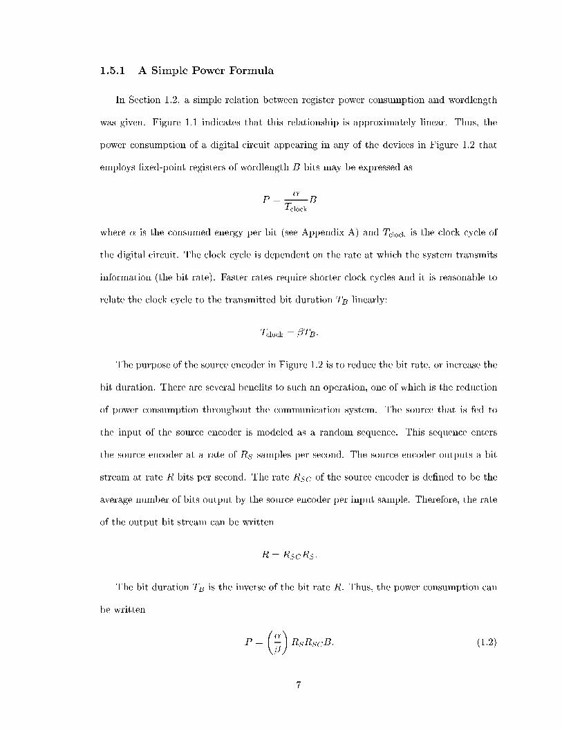
1.5.1 A Simple Power Formula
In Section 1.2, a simple relation between register power consumption and wordlength
was given. Figure 1.1 indicates that this relationship is approximately linear. Thus, the
power consumption of a digital circuit appearing in any of the devices in Figure 1.2 that
employs �xed-point registers of wordlength B bits may be expressed as
P =�
TclockB
where � is the consumed energy per bit (see Appendix A) and Tclock is the clock cycle of
the digital circuit. The clock cycle is dependent on the rate at which the system transmits
information (the bit rate). Faster rates require shorter clock cycles and it is reasonable to
relate the clock cycle to the transmitted bit duration TB linearly:
Tclock = �TB :
The purpose of the source encoder in Figure 1.2 is to reduce the bit rate, or increase the
bit duration. There are several bene�ts to such an operation, one of which is the reduction
of power consumption throughout the communication system. The source that is fed to
the input of the source encoder is modeled as a random sequence. This sequence enters
the source encoder at a rate of RS samples per second. The source encoder outputs a bit
stream at rate R bits per second. The rate RSC of the source encoder is de�ned to be the
average number of bits output by the source encoder per input sample. Therefore, the rate
of the output bit stream can be written
R = RSCRS :
The bit duration TB is the inverse of the bit rate R. Thus, the power consumption can
be written
P =
��
�
�RSRSCB: (1.2)
7

In equation (1.2), the source encoder rate RSC and the register wordlength B are design
parameters. The equation clearly shows that both quantities must be minimized to achieve
low power consumption. As may be expected, reduction of either design parameter has an
adverse e�ect on system performance. The designer must therefore optimize performance
subject to power consumption constraints. The fundamental objectives of this dissertation
are to develop relations between system performance and the design parameters (wordlength
and source code rate) and to develop techniques whereby these relations may be utilized to
optimize performance subject to power constraints.
1.5.2 Wordlength Reduction
Many of the digital subsystems shown in Figure 1.2 are �xed-point units that perform
signal processing algorithms in e�orts to transmit or receive data reliably. The majority of
the signal processing algorithms performed by the digital subsystems of a communication
system are well understood and can be analyzed elegantly and rigorously. Such analysis,
however, is often greatly complicated by introduction of �xed-point e�ects. It is always
true that increased wordlengths correspond to improved performance, but the quantitative
relationship between the two is almost never known. The designer, then, often resorts to
trial-and-error methods to select the optimal wordlength to meet a given power constraint.
Low-Power LMS Adaptation
In Chapter 2, reduced wordlength e�ects are investigated for �xed-point adaptive chan-
nel equalizers employing the Least Mean Squares (LMS) algorithm. The relationship be-
tween the algorithm's performance, as measured by its transient behavior and steady-state
mean square error (MSE), is determined. A design procedure is then developed whereby
the algorithm can be optimized for minimum steady-state MSE subject to a constraint on
its power consumption.
8

1.5.3 Source Encoding
Power consumption can be reduced in all digital processing units of a communication
system by reducing the source encoder rate RSC . The relationship between the rate and
distortion of a source encoder has been studied extensively. Indeed an entire branch of
information theory is devoted to so-called rate-distortion theory. When designing a lossy
source encoder and decoder, the objective is to achieve a low rate while minimizing the
distortion. The measure of distortion that is to be minimized must be selected carefully and
intelligently based upon the intended application of the reconstructed signal. For instance,
a speech encoder must be designed so that the reconstructed signal is perceived to be very
similar to the source.
Vector Quantization for Distributed Hypothesis Testing
In Chapter 3, the problem of source coding for hypothesis testing applications is studied.
Vector quantization is selected as the source coding technique and it is shown that, in some
cases, a quantizer can achieve a very low rate while sacri�cing no loss in performance of the
hypothesis test for which the reconstructed data is intended. For the cases in which such
quantizers do not exist, optimal quantizers are derived, for a given rate, that minimize the
loss in area under an analog to the receiver operating characteristic (ROC) curve of the
Neyman-Pearson hypothesis test.
9

CHAPTER 2
Low-Power LMS Adaptation
2.1 Introduction
The Least Mean Squares (LMS) algorithm, introduced by Widrow and Ho� [71, 74],
�nds itself in many components of a digital communication system. The relative simplicity
of the algorithm renders it ideal for adaptive channel equalization and estimation [67],
adaptive beamforming antenna arrays [72], and adaptive interference cancellation systems
[25]. The near ubiquity of the algorithm in digital communications along with the ever-
increasing demand for low-power communication systems warrants an understanding of
the relationship between its performance and power consumption. Indeed, a great deal of
research has been done on the LMS algorithm's behavior over the years [65], but very little
of this work has focused on the power-performance relationship.
Insight into the LMS algorithm's power-performance relationship is of paramount im-
portance for low-power LMS implementation. Without such insight, the system designer
must resort to exhaustive trial-and-error methods to achieve low power consumption. Con-
versely, equipped with an understanding of LMS power-performance behavior, the designer
may optimize an LMS system's performance given a power constraint, or vice-versa.
To illustrate more speci�cally the motivation for low-power LMS implementation, con-
sider a battery-powered wireless receiver, for which the adaptive LMS equalization function
consumes a signi�cant portion of the total battery power. As an example, the SINCGARS
combat radio used by the United States Army consumes on the average 7 Watts in receive
10

mode, of which more than 1 Watt (over 14% of total power) is consumed by the channel
equalizer [44]. Clearly then, the equalization function is a prime target for power reduction
in these handsets.
Many digital hardware design strategies have been proposed for power reduction includ-
ing: reduction of supply voltage, reduction of clock speed and data rate, parallelization and
pipelining of operations, using sign-magnitude arithmetic, and di�erential encoding of data
[16, 51]. Another technique is the reduction of the number of bits (wordlength) used to rep-
resent the data and control variables in the digital circuit [52]. The wordlength reduction
strategy is very highly leveraged since it reduces the power dissipation everywhere in the
data and control ow paths. This strategy is also very versatile since it can be applied to
any hardware architecture and can be easily adjusted in real time by dynamically disabling
bus lines and register bits.
As mentioned previously, power reduction { by means of wordlength reduction or any
other technique { must be carried out with foresight regarding algorithm performance. For
example, LMS wordlength reduction generally entails a degradation in algorithm perfor-
mance as measured by adaptive algorithm convergence rate and steady-state mean square
error (MSE). This chapter provides an analysis of MSE degradation versus power reduction,
by means of coeÆcient and data wordlength reduction, for the LMS algorithm. Addition-
ally, optimization of the algorithm under a power constraint is described and illustrated for
the case of channel equalization.
2.1.1 The LMS Algorithm
The LMS algorithm iteratively adapts the coeÆcients of an FIR �lter in an attempt to
minimize the mean-square value of an error signal formed by subtracting the �ltered output
from a primary, or desired, signal. In a digital implementation, all signals and coeÆcients are
stored with �nite precision. Most �nite-precision implementations use �xed-point registers.
The �nite-precision LMS algorithm can be viewed as an in�nite-precision LMS algorithm
11
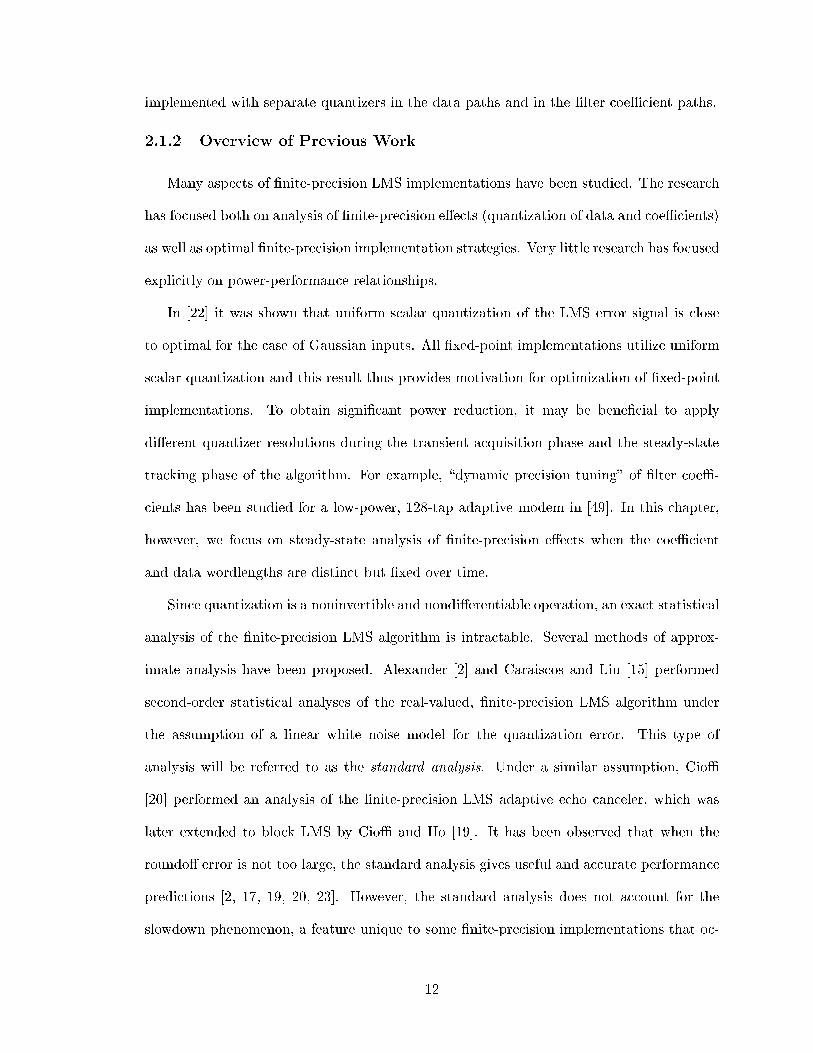
implemented with separate quantizers in the data paths and in the �lter coeÆcient paths.
2.1.2 Overview of Previous Work
Many aspects of �nite-precision LMS implementations have been studied. The research
has focused both on analysis of �nite-precision e�ects (quantization of data and coeÆcients)
as well as optimal �nite-precision implementation strategies. Very little research has focused
explicitly on power-performance relationships.
In [22] it was shown that uniform scalar quantization of the LMS error signal is close
to optimal for the case of Gaussian inputs. All �xed-point implementations utilize uniform
scalar quantization and this result thus provides motivation for optimization of �xed-point
implementations. To obtain signi�cant power reduction, it may be bene�cial to apply
di�erent quantizer resolutions during the transient acquisition phase and the steady-state
tracking phase of the algorithm. For example, \dynamic precision tuning" of �lter coeÆ-
cients has been studied for a low-power, 128-tap adaptive modem in [49]. In this chapter,
however, we focus on steady-state analysis of �nite-precision e�ects when the coeÆcient
and data wordlengths are distinct but �xed over time.
Since quantization is a noninvertible and nondi�erentiable operation, an exact statistical
analysis of the �nite-precision LMS algorithm is intractable. Several methods of approx-
imate analysis have been proposed. Alexander [2] and Caraiscos and Liu [15] performed
second-order statistical analyses of the real-valued, �nite-precision LMS algorithm under
the assumption of a linear white noise model for the quantization error. This type of
analysis will be referred to as the standard analysis. Under a similar assumption, CioÆ
[20] performed an analysis of the �nite-precision LMS adaptive echo canceler, which was
later extended to block LMS by CioÆ and Ho [19]. It has been observed that when the
roundo� error is not too large, the standard analysis gives useful and accurate performance
predictions [2, 17, 19, 20, 23]. However, the standard analysis does not account for the
slowdown phenomenon, a feature unique to some �nite-precision implementations that oc-
12

curs when the LMS weights do not get regularly updated due to excessive roundo� error.
For the special case of the LMS algorithm implemented with �nite-precision coeÆcients
and in�nite-precision data, Bermudez and Bershad [6, 7, 8] presented a recursive learning
curve approximation that gives more accurate predictions of the steady-state MSE than the
standard analysis, the standard analysis giving increasingly poor predictions as coeÆcient
resolution decreases.
2.1.3 Overview of Contribution
In this chapter, we use the standard analysis methodology to derive expressions for op-
timal bit allocation factors for �nite-precision LMS implementations that do not experience
slowdown under total data + coeÆcient wordlength constraints and total power constraints.
As a check against the presence of slowdown, we propose a simple and accurate criterion
that predicts that slowdown will not occur when the number of coeÆcient bits exceeds the
number of data bits by a quantity speci�ed by the criterion. This conclusion is based on
extensive numerical simulations of �nite-precision LMS for channel equalization and system
identi�cation, as well as analytical studies. While the results are directly applicable to
the generic �nite-precision LMS algorithm in a variety of applications, for concreteness we
concentrate on the case of channel equalization with training.
An outline of the chapter is as follows. We begin with a preliminary overview of the
in�nite-precision LMS algorithm along with a mathematical description of our model for
the �nite-precision algorithm in Sections 2.2.1 and 2.2.2. In Section 2.2.3, we derive a for-
mula for the iteration power of the �xed-point, power-of-two step-size LMS algorithm under
�xed-point complex arithmetic, cyclic updating of the data stack, and table lookup imple-
mentation of multiplication. Next, in Section 2.2.4, using the averaged system techniques of
Solo and Kong [65], we obtain analytical expressions for the increase in steady-state mean
square error due to �nite precision in the absence of the slowdown phenomenon which gen-
eralize the formulas of Caraiscos and Liu [15] to the case of complex data and coeÆcients.
13

yk
?xk- FIR �lter
yk- j�
LMS
wk
6
- ek�
Figure 2.1: In�nite-precision LMS algorithm.
We also present a simple constraint on the data wordlength, coeÆcient wordlength, and
adaptation step size � that prevents the slowdown phenomenon. We then derive a pair
of optimal bit allocation factors, in Section 2.3, that minimize the amount of increase in
MSE subject to two constraints: 1) a total bit width constraint (total bit budget) and 2)
a total power consumption constraint (total power budget). We conclude that assigning
more bits to coeÆcients than data is necessary to avoid the slowdown phenomenon and in
general gives better steady-state MSE performance under a total power budget constraint.
This conclusion mirrors a similar result reported in [23] for the �nite-precision sign LMS
algorithm. Finally, in Section 2.4, we verify the accuracy of our theoretical predictions for
the case of LMS equalization of a single-pole IIR channel.
2.2 Finite-Precision LMS Adaptation
2.2.1 In�nite-Precision LMS Algorithm
Figure 2.1 shows a block diagram of the in�nite-precision LMS algorithm. Here yk
is a complex training signal, xk is the complex FIR �lter input, and yk = wHk xk is a
linear estimate of yk given the p samples xk = [xk; : : : ; xk�p+1]T and �lter coeÆcients
wk = [w0;k; : : : ; wp�1;k]H . Note that the FIR �lter has p taps. The signal ek = yk � yk is
the error signal whose mean-square value the algorithm attempts to minimize. The vehicle
by which this minimization is accomplished is a recursive coeÆcient update, �rst derived
14
sk-Qd
s0k - ay0k
?xk-Qd
-x0k
FIR �lter -Qd
y0k- j�
Qc
w0k6
LMS
6
- e0k�
�� -1=as0k-
Figure 2.2: Finite-precision LMS algorithm.
by Widrow and Ho� [71, 73, 74]. The recursion seeks the minimum of the MSE surface
E[jekj2] = E[jyk � wHk xkj2] by means of gradient descent with an estimated gradient. The
recursion is given by
wk+1 = wk + �xke�k
ek = yk � yk (2.1)
where � is the adaptive gain parameter that controls the convergence properties of the
algorithm and � denotes complex conjugation.
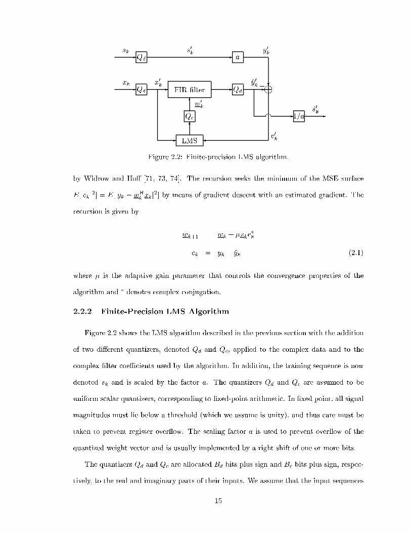
2.2.2 Finite-Precision LMS Algorithm
Figure 2.2 shows the LMS algorithm described in the previous section with the addition
of two di�erent quantizers, denoted Qd and Qc, applied to the complex data and to the
complex �lter coeÆcients used by the algorithm. In addition, the training sequence is now
denoted sk and is scaled by the factor a. The quantizers Qd and Qc are assumed to be
uniform scalar quantizers, corresponding to �xed-point arithmetic. In �xed point, all signal
magnitudes must lie below a threshold (which we assume is unity), and thus care must be
taken to prevent register over ow. The scaling factor a is used to prevent over ow of the
quantized weight vector and is usually implemented by a right shift of one or more bits.
The quantizers Qd and Qc are allocated Bd bits plus sign and Bc bits plus sign, respec-
tively, to the real and imaginary parts of their inputs. We assume that the input sequences
15

have been scaled to lie between �1 and +1. As in [15], we assume that the e�ect of the oper-
ators Qd and Qc is to add to their inputs complex white noises of variance 2�2d = (1=6)2�2Bd
for Qd and 2�2c = (1=6)2�2Bd for Qc.
The �nite-precision LMS algorithm implements the recursion (2.1) with quantizers in
all data paths as shown in Figure 2.2. The �nite-precision recursion can be written as
w0k+1 = w0k +Qc
�� x0ke
0�k
�(2.2)
where
e0k = y0k �Qd
�w0Hk x0k
�(2.3)
is the quantized error signal. We assume that the gain parameter � is chosen to be a power
of two, thereby enabling the multiplication by � to be performed by right shifts. We have
used primed symbols to represent quantized values. For example, x0k = Qd(xk) is simply
the quantized value of the FIR �lter input. Similarly, s0k = Qd(sk). For the coeÆcients, w0k
represents the value of the weight vector used in the �nite-precision algorithm at iteration
k. Note that this should approximate wk, the weight vector at iteration k of the in�nite-
precision algorithm, if the input signals are the same. We assume that the computation of
the inner product in (2.3) is accomplished by quantizing the partial sums. Therefore,
Qd(w0Hk x0k) =
p�1Xi=0
Qd(w0i;kx
0k�i)
and the noise added to the inner product has variance 2p�2d.
2.2.3 Power Consumption of LMS Algorithm
The total iteration power of the �nite-precision LMS algorithm is determined by power
dissipation of shift, add, multiply, memory load, and memory store operations. This depends
on the speci�c circuit implementation of the FIR �lter and control circuitry. The bulk of
the power dissipation usually comes from add and multiply operations. In Appendix B, we
derive the following formula for iteration power of LMS considering only adds and multiplies
16

under the assumption that � = 2�q for q 2 f0; : : : ; Bc � 1g:
PT = 4p[(2Bd +Bc + 2)�a + (3Bd +Bc)�t]: (2.4)
This expression is linear in the number of bits Bd and Bc and assumes �xed-point complex
arithmetic, cyclic updating of the data stack [xk; : : : ; xk�p+1]T by overwriting xk�p+1 with
xk+1, and multiplication using table lookup as opposed to adding partial products. In (2.4),
we have de�ned generic power coeÆcients �a and �t representing power consumption per
add per bit and power consumption per table lookup operation per bit, respectively.
2.2.4 Statistical Performance of Finite-Precision LMS Algorithm
The performance of the LMS adaptive algorithm is typically characterized by two quan-
tities: the speed of convergence and the excess MSE [65, 67, 74]. We assume that sk and
xk are both wide-sense stationary random sequences. Caraiscos and Liu [15] analyzed the
e�ects of �nite wordlength on (real-valued) LMS �lter performance under the following high
resolution assumptions:
The quantization errors of quantizers Qd and Qc are zero
mean, white, with variances 2�2d and 2�2c , respectively. Fur-
thermore, these errors are independent of the quantizer in-
puts. The process xk is circular Gaussian. The step size � is
greater than 0 and Bc, Bd � 1. Finally, the sequences sk and
xk have been scaled so that they do not over ow.
(2.5)
In the remainder of this section, we derive the mean convergence rate, steady-state weight-
error covariance, and excess mean square error for complex-valued, �nite-precision LMS
under the above assumptions. As will be shown below, use of these assumptions yields
accurate error predictions when slowdown does not occur. Later, we derive constraints on
Bc, Bd, and � that prevent the occurance of slowdown.
17
Mean Convergence
De�ne the p � p covariance matrix Rx0 = E[x0kx0Hk ] of the quantized data and let this
matrix have real, non-negative eigenvalues f�0igpi=1. Further, de�ne the cross correlation
vector Rx0y0 = E[x0ky0�k ]. Assume the gain parameter � satis�es the condition
0 < j1� ��0ij < 1; i = 1; : : : ; p: (2.6)
In Appendix C.1, we show that the �lter coeÆcients of the �nite-precision LMS algorithm
converge in the mean to a set of optimal weights w0o called the (�nite-precision) Wiener
weights:
limk!1
E[w0k] = w0o (2.7)
where
w0o = R�1x0 Rx0y0 :
When the �nite-precision LMS algorithm converges, its MSE trajectory, or learning
curve, converges as a decaying exponential with the 1=e time constant of the slowest mode
equal to �3dB = 1=(�maxi ln(j1 � ��0ij)), called the adaptation time constant. Note that
the speed of convergence generally increases as � increases.
Steady-State Weight-Error Covariance
In Appendix C.2, we derive an expression for the steady-state quantized weight-error
covariance. Let Pk = E[(w0k�wk)(w0k�wk)
H ] where wk is the weight vector at iteration k of
the in�nite-precision LMS algorithm. Then, assuming Pk converges as k !1, it converges
to the steady-state covariance matrix given by
P = �(p+ 1)�2dI +1
��2cR
�1x0 : (2.8)
Excess Mean Square Error
De�ne the in�nite-precision covariance matrix Rx = E[xkxHk ] and cross correlation
vector Rxy = E[xky�k]. Under the assumptions (2.5), the following asymptotic expression
18

for the steady-state mean square error is derived for small � in Appendix C.2:
� = E[jsk � s0kj2] = �min + �excess + �q (2.9)
where
�min =1
a2��2y �RH
xyR�1x Rxy
�
is the optimal mean square error with the in�nite-precision Wiener weights wo,
�excess =1
2�tr(Rx)�min
is the excess MSE due to misadjustment, and
�q = �c 2�2Bc + �d 2
�2Bd (2.10)
where
�c =p
12�a2; �d =
kwok2 + p
6a2
and wo = R�1x Rxy is the optimal Wiener weight vector for the standard, in�nite-precision,
complex LMS algorithm.
The term �q is the excess MSE due to quantization of the data and �lter coeÆcients.
The �rst term in the expression (2.10) is the excess MSE due only to quantization of the
�lter coeÆcients while the second term represents the MSE due to quantization of the data.
Note that for small � the term �c dominates the excess MSE due to quantization unless
Bc is made large. This implies that for small step sizes a high resolution is required for the
�lter coeÆcients. Also worth noting is that �q increases in p at a linear rate, decreases in
� at an inverse linear rate, and decreases in Bd and Bc at an exponential rate. Therefore,
the total number of bits allocated gives more leverage over excess MSE than any other of
the design parameters.
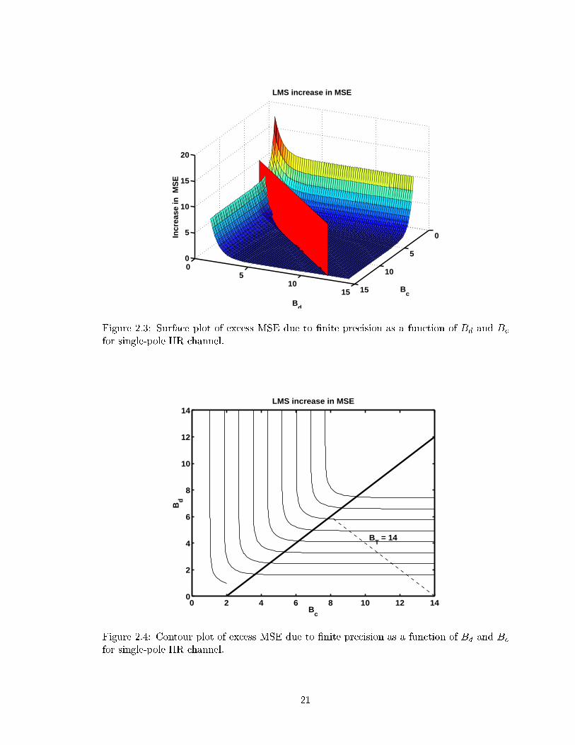
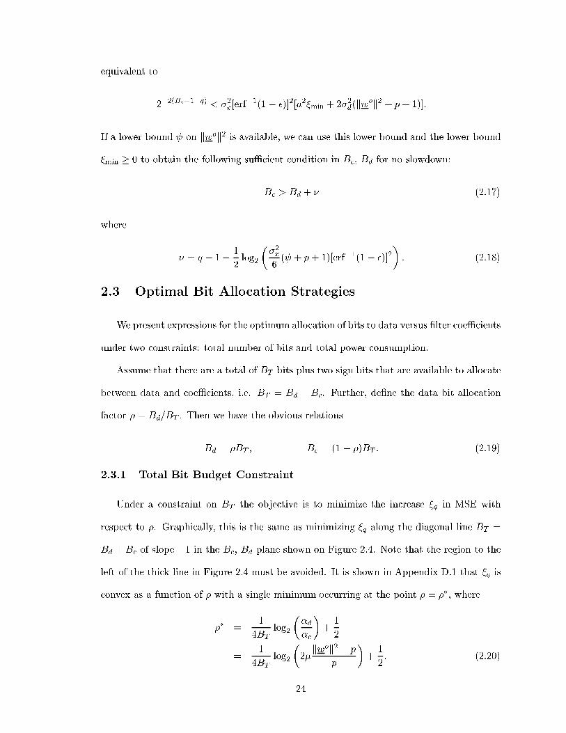
With these relations, the increase in MSE due to �nite precision �q can be plotted as a
function of Bd and Bc. A plot of the increase in MSE is given in Figures 2.3 and 2.4 for
19

the case of white sk and for xk generated by passing sk through a single-pole IIR �lter with
pole at a1 = 0:8 and with LMS gain parameter � = 1=4, scaling factor a = 1=8, and p = 2
taps. The vertical plane on the surface plot and the thick line on the contour plot divide
the Bc, Bd plane into two regions. In the next section, we will show that the value �q is
valid only in the region to the left of the vertical plane in Figure 2.3 (right of the thick line
in Figure 2.4) while the other region is the slowdown region.
Predicting Onset of Slowdown
The slowdown phenomenon occurs when one or more components of the input to the
quantizer Qc in (2.2) falls below the LSB of Qc [6, 7, 15, 28]. The corresponding onset of
slowdown can be de�ned as the minimum integer k > 0 such that
��Ref�x0k�ie0�k g�� < �c
2or
��Imf�x0k�ie0�k g�� < �c
2(2.11)
for some i 2 f0; : : : ; p � 1g. Here Ref�g and Imf�g denote real and imaginary parts and
�c = 2�Bc is the granularity of the coeÆcient quantizer. During the initial stages of
adaptation, before onset of slowdown, the �nite-precision LMS algorithm's behavior does
not di�er signi�cantly from that of the in�nite-precision algorithm [6, 7]. When condition
(2.11) is met at iteration k, at least one of the complex components of the ith element of the
vector w0k does not get updated and the �nite-precision algorithm's learning curve begins
to diverge from that of the in�nite-precision algorithm. To determine the point at which
this divergence occurs, called the slowdown point, consider the probability
maxi=0;:::;p�1
P
���Ref�x0k�ie0�k g�� < �c
2
�> 1� � (2.12)
for 0 < � � 1. It is easily shown that the left-hand side of (2.12) is a lower bound on the
joint probability of the event (2.11). Furthermore, the left-hand side completely speci�es
this joint probability when xk is independent and identically distributed (i.i.d.) with i.i.d.
real and imaginary parts. Thus, if for some k (2.12) is satis�ed, then with probability
at least 1 � � the iteration k is a slowdown point. Furthermore, we can assert that if no
20
0
5
10
15
05
1015
0
5
10
15
20
Bc
LMS increase in MSE
Bd
Incr
ease
in M
SE
Figure 2.3: Surface plot of excess MSE due to �nite precision as a function of Bd and Bc
for single-pole IIR channel.
0 2 4 6 8 10 12 140
2
4
6
8
10
12
14
Bc
Bd
LMS increase in MSE
BT = 14
Figure 2.4: Contour plot of excess MSE due to �nite precision as a function of Bd and Bc
for single-pole IIR channel.
21

iteration k satis�es (2.12) before steady-state is reached, then slowdown will not occur with
probability at least 1��. These observations are the basis for our approach to prevention of
slowdown: determine the minimum value of �c that ensures that (2.12) can only be satis�ed
after steady-state is reached. This value of �c will then specify a range of admissible values
for Bc, Bd, and � for which slowdown does not occur. The choice of � will be discussed in
Section 2.4.
The condition (2.12) will be evaluated by invoking the fact that the �nite-precision
algorithm's behavior does not di�er signi�cantly from that of the in�nite-precision algorithm
before slowdown and therefore (2.12) can be replaced by
maxi=0;:::;p�1
P
�jRef�xk�ie�kgj <
�c
2
�> 1� � (2.13)
where ek = yk � yk is the error signal in the in�nite-precision algorithm. Now de�ne gk =
xk�ie�k and make the simplifying assumption that gk is approximately circular Gaussian with
mean zero and variance �2x�2e;k where �
2x = E[jxkj2] and �2e;k = E[jekj2] is the mean square
error of the in�nite-precision algorithm. Before slowdown we have �2e;k � �0k = E[je0kj2].
Then (2.13) predicts that slowdown will begin (with probability at least 1 � �) when k
satis�es
erf
�c
2��xp�0k
!= 1� �:
This is equivalent to
�0k =2�2(Bc+1�q)
�2x[erf�1(1� �)]2
= �0slow (2.14)
where q = � log2 �.
Now, from the de�nition of e0k and the results of the previous section, we have �01 =
a2� + 2�2d in the absence of slowdown. Therefore, assuming no slowdown, for a �xed Bd
�01 > a2(�min + �excess + �qjBc=1) + 2�2d
22

0 1000 2000 3000 4000 500010
−10
10−8
10−6
10−4
10−2
100
Iteration Number, k
MS
E
Finite Precision LMS with Slowdown
Bc = B
d = 10
Infinite Precisionξ’
slow
ξ’floor
Figure 2.5: Example of slowdown.
and assuming � is small
�01 > a2�min + 2�2d(kwok2 + p+ 1)
= �0 oor: (2.15)
Figure 2.5 shows a sample learning curve of a �nite-precision LMS channel equalizer that
experiences slowdown along with the values �0slow and �0 oor.
Again, since the �nite and in�nite-precision algorithms agree closely before onset of
slowdown, slowdown can be prevented by choosing Bc such that
�0slow < �0 oor: (2.16)
Note from the derivation of �0slow that this quantity is the minimum value of �0k achievable
before the onset of slowdown with in�nite-precision data. The MSE �0 oor is the steady-
state MSE (in the absence of slowdown) with in�nite-precision coeÆcients. Thus, if Bc and
Bd are chosen such that the inequality (2.16) is satis�ed, then with high probability the
slowdown MSE �0slow will not be reached and slowdown will not occur. Inequality (2.16) is
23
equivalent to
2�2(Bc+1�q) < �2x[erf�1(1� �)]2[a2�min + 2�2d(kwok2 + p+ 1)]:
If a lower bound on kwok2 is available, we can use this lower bound and the lower bound
�min � 0 to obtain the following suÆcient condition in Bc, Bd for no slowdown:
Bc > Bd + � (2.17)
where
� = q � 1� 1
2log2
��2x6( + p+ 1)[erf�1(1� �)]2
�: (2.18)
2.3 Optimal Bit Allocation Strategies
We present expressions for the optimum allocation of bits to data versus �lter coeÆcients
under two constraints: total number of bits and total power consumption.
Assume that there are a total of BT bits plus two sign bits that are available to allocate
between data and coeÆcients, i.e. BT = Bd + Bc. Further, de�ne the data bit allocation
factor � = Bd=BT . Then we have the obvious relations
Bd = �BT ; Bc = (1� �)BT : (2.19)
2.3.1 Total Bit Budget Constraint
Under a constraint on BT the objective is to minimize the increase �q in MSE with
respect to �. Graphically, this is the same as minimizing �q along the diagonal line BT =
Bd +Bc of slope �1 in the Bc, Bd plane shown on Figure 2.4. Note that the region to the
left of the thick line in Figure 2.4 must be avoided. It is shown in Appendix D.1 that �q is
convex as a function of � with a single minimum occurring at the point � = ��, where
�� =1
4BTlog2
��d�c
�+1
2
=1
4BTlog2
�2�kwok2 + p
p
�+1
2: (2.20)
24

Observe that as BT increases, �� approaches the standard textbook allocation of 1/2. How-
ever, for low BT the standard allocation is suboptimal.
Note that condition (2.17) is equivalent to
� <1
2� �
2BT= �slow: (2.21)
Therefore, since �q is convex as a function of �, the optimal value of � is
�B = minf��; �slowg:
2.3.2 Total Power Budget Constraint
Under a constraint on total power budget PT , we can use (2.4) and (2.19) to re-express
the total combined number of bits BT as a function of � and PT :
BT =PT � 8p�a
4p[�(�a + 2�t) + �a + �t]: (2.22)
In Appendix D.2 we show that for BT � 2, �q is once again a convex function of � with
unique minimum at � = ���, where
��� =PT � 8p�a + 2p(�a + �t) log2
h�d�c� �a+�t2�a+3�t
i2(PT � 8p�a)� 2p(�a + 2�t) log2
h�d�c� �a+�t2�a+3�t
i : (2.23)
Similar to the bit budget constraint, ��� converges to the standard 1/2 allocation as PT
becomes large while for low PT the standard allocation is suboptimal.
Again applying constraint (2.17) the optimal allocation is
�P = minf���; �slowg
where �slow is calculated using (2.21) and (2.22).
2.4 Numerical Example
Here we brie y consider LMS equalization of an IIR channel with a single pole at
a1 = 0:5, a Gaussian transmitted signal sk with variance E[jskj2] = �2s = 0:06, a Gaussian-
noise-corrupted training sequence yk = sk + nk with E[jnkj2] = �2n = 10�8, and a two-tap
25
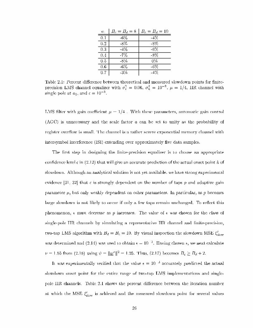
a1 Bc = Bd = 8 Bc = Bd = 10
0.1 -6% -4%
0.2 -8% -8%
0.3 -4% -6%
0.4 -7% -8%
0.5 -8% 0%
0.6 -6% -6%
0.7 -3% -4%
Table 2.1: Percent di�erence between theoretical and measured slowdown points for �nite-precision LMS channel equalizer with �2s = 0:06, �2n = 10�8, � = 1=4, IIR channel withsingle pole at a1, and � = 10�3.
LMS �lter with gain coeÆcient � = 1=4 . With these parameters, automatic gain control
(AGC) is unnecessary and the scale factor a can be set to unity as the probability of
register over ow is small. The channel is a rather severe exponential memory channel with
intersymbol interference (ISI) extending over approximately �ve data samples.
The �rst step in designing the �nite-precision equalizer is to choose an appropriate
con�dence level � in (2.12) that will give an accurate prediction of the actual onset point k of
slowdown. Although an analytical solution is not yet available, we have strong experimental
evidence [31, 32] that � is strongly dependent on the number of taps p and adaptive gain
parameter �, but only weakly dependent on other parameters. In particular, as p becomes
large slowdown is not likely to occur if only a few taps remain unchanged. To re ect this
phenomenon, � must decrease as p increases. The value of � was chosen for the class of
single-pole IIR channels by simulating a representative IIR channel and �nite-precision,
two-tap LMS algorithm with Bd = Bc = 10. By visual inspection the slowdown MSE �0slow
was determined and (2.14) was used to obtain � = 10�3. Having chosen �, we next calculate
� = 1:85 from (2.18) using = kwok2 = 1:25. Thus, (2.17) becomes Bc � Bd + 2.
It was experimentally veri�ed that the value � = 10�3 accurately predicted the actual
slowdown onset point for the entire range of two-tap LMS implementations and single-
pole IIR channels. Table 2.1 shows the percent di�erence between the iteration number
at which the MSE �0slow is achieved and the measured slowdown point for several values
26

0 500 1000 1500 2000
10−8
10−7
10−6
Bd = 11, B
c = 13
Iteration Number, k
MS
E
Finite Precision LMS Learning Curves
Bd = 12, B
c = 14
Bd = 13, B
c = 15
ξk Experimental
ξ Theoretical
Figure 2.6: Learning curves of LMS �lters equalizing IIR channel with Gaussian inputwithout slowdown.
of the channel pole a1. The table shows that using � = 10�3 yields accurate slowdown
point predictions for di�erent wordlengths and channels. Note that since the di�erences are
all non-positive, the estimate �0slow and the constraint Bc > Bd + � are both conservative.
Figure 2.6 shows a representative sampling of the learning curves for di�erent �nite-precision
equalizers satisfying (2.17) along with the predicted value of the steady-state MSE given by
(2.9). Again, choice of � = 10�3 has yielded a constraint preventing slowdown for various
wordlengths.
To determine the power coeÆcients �a and �t for this example, several adders and
multipliers with varying bit-width were simulated using the Epoch CAD package. The
energy consumption of each adder and multiplier was determined and by using linear least
squares �ts to this data, the adder energy per bit and multiplier energy per bit were obtained.
These �gures were then multiplied by the assumed clock cycle of 50 MHz to give the
coeÆcients �a � 1:4 mW and �t � 6:8 mW. The simulated multipliers were shift-add
(partial product) multipliers. Although our analysis considers table lookup multipliers, it
is clear from Figure B.1 that the chosen value of �t gives a good power approximation for
either multiplier.
27

10 15 20 25 300.3
0.35
0.4
0.45
0.5
0.55
Bit Allocation vs. BT
BT
ρ* ρ
slow
Figure 2.7: IIR channel with Gaussian input: data bit allocation factors underBT constraintas functions of BT .
Figure 2.7 shows the BT -constrained data bit allocation factor �� as a function of BT
as well as �slow, the maximum allowable allocation satisfying (2.17). It is clear that for all
BT , �slow < �� and therefore the optimal allocation factor is �B = �slow. Figure 2.8 shows
the PT -constrained data bit allocation factor ��� as a function of PT as well �slow. Again
note that for all PT of interest, �slow < ��� and the optimal allocation factor is �P = �slow.
Also shown on this �gure are two suboptimal allocations, each satisfying the no-slowdown
constraint. Finally, Figure 2.9 shows the resultant MSE � as a function of PT using the
optimal allocation � = �P = �slow as well as the suboptimal allocations plotted on a log
scale.
While these results show that the bit allocation �slow is always optimal for this example,
it should be noted that this is not always the case. For example, consider the design of a
�nite-precision LMS equalizer with the following parameters: p = 32, kwok2 = 1, a = 1,
� = 1=8, �2s = 0:06, �2x = 0:09. Using � = 10�5 (the correct value for these parameters),
Figures 2.10 and 2.11 show that for this case the optimal bit allocation factors are �� and
28
1 1.5 2 2.5 3 3.50.3
0.35
0.4
0.45
0.5
0.55
0.6
PT (Watts)
Bit
Allo
catio
n F
acto
r
Bit Allocation vs. PT
ρ = ρ** ρ = ρ
slow
Bc = B
d + ν + 2
ρ = 1/3
Figure 2.8: IIR channel with Gaussian input: data bit allocation factors under PT constraintas functions of PT .
1.4 1.6 1.8 2 2.2 2.4 2.6 2.8 310
−7
10−6
10−5
10−4
10−3
PT (Watts)
MS
E, ξ
MSE vs. PT with Various Allocations
ρ = ρslow
B
c = B
d + ν + 2
ρ = 1/3
Figure 2.9: IIR channel with Gaussian input: MSE as function of PT for various bit alloca-tions.
29

10 15 20 25 300.3
0.35
0.4
0.45
0.5
0.55
Bit Allocation vs. BT
BT
ρ* ρ
slow
Figure 2.10: 32-tap LMS channel equalizer: data bit allocation factors under BT constraintas functions of BT .
15 20 25 30 35 40 45 50 550.3
0.35
0.4
0.45
0.5
0.55
0.6
PT (Watts)
Bit
Allo
catio
n F
acto
r
Bit Allocation vs. PT
ρ = ρ** ρ = ρ
slowρ = 1/3
Figure 2.11: 32-tap LMS channel equalizer: data bit allocation factors under PT constraintas functions of PT .
30

25 30 35 40 45 5010
−6
10−5
10−4
10−3
10−2
PT (Watts)
MS
E, ξ
MSE vs. PT with Various Allocations
ρ = ρ** ρ = ρ
slowρ = 1/3
Figure 2.12: 32-tap LMS channel equalizer: MSE as function of PT for various bit alloca-tions.
���. Figure 2.12 shows the MSE as a function of PT for this case with � = �slow and � = ���.
Observe that, as expected, the MSE with ��� attains the minimum.
2.5 Conclusion
In this chapter, a design methodology has been developed by which low-power imple-
mentation of LMS adaptive channel equalizers can be achieved. Expressions have been
derived for optimal bit allocation under combined register length constraints and total
power constraints while avoiding the slowdown phenomenon. These expressions can easily
be specialized to a speci�c hardware implementation for computation of the number of bits
to allocate to data and �lter coeÆcients. A general conclusion is that the standard design
strategy of allocating an equal number of bits to the data and �lter coeÆcients is optimal
only as the power or register length constraints become very large. Furthermore, this 50%
allocation can yield undesired slowdown in the transient phase of adaptation. For most
LMS implementations, it is optimal to allocate more bits to the �lter coeÆcients than to
the data.
31

It is important to emphasize that the linear steady-state analysis presented in this
chapter is relevant only for implementations of LMS for which slowdown does not occur,
i.e. for the cases that wordlength satis�es the condition (2.17). To optimize performance
over all possible choices of wordlengths, including those for which slowdown occurs, a full,
nonlinear, �nite-precision analysis of LMS must be performed. For example, the methods
of [6, 7, 8] might be applied if they could be extended to cover the case where both data
and coeÆcients are �nite precision.
32

CHAPTER 3
Vector Quantization for Distributed Hypothesis Testing
3.1 Introduction
In a myriad of applications, the intent of data transmission is for a user to make a
decision, or hypothesis test, based upon the received data. For example, a radar sensor
must transmit information to a user for determination of a target's presence. The optimality
criterion by which the source encoder is designed must be directly related to the performance
of the receiver's decision rule in these cases. In most communication systems, the source
encoder objective function is the mean square error (MSE). This criterion is suitable when
it is desired that the received data be an accurate estimate of the transmitted data. Thus, a
source encoder designed for minimum MSE can be considered an estimation-optimal source
encoder. Mean square error, however, is not the most suitable criterion for hypothesis
testing. Type I and type II error probabilities are more conventional gauges of performance
for hypothesis tests. A source encoder for hypothesis testing applications should therefore
be designed with the error probabilities as minimization criteria. As hypothesis testing
often consists of detection of a target, such a source encoder could be considered a detection-
optimal source encoder. Detection performance can never improve with source encoding and
the loss in detection performance will certainly be small when a source encoder with excellent
estimation performance (low MSE) is used. However, as design of an estimation-optimal
source encoder is in no way in uenced by the hypothesis test for which the reconstructed
data is intended, such an encoder may unnecessarily sacri�ce rate, in the form of transmitted
33

H0
H1
Environment
vm
vm
...
vm
Sensors
-
-
-
x(1)
x(2)
x(n)
Q1
Q2
Qn
...
Quantizers
-
-
-
C1
C2
Cn
...
Channels
-
-
-
x(1)
x(2)
x(n)
�(x)
Test Statistic
-��
@@ ��
@@? T
e
e
\H0"
\H1"
Figure 3.1: Sensor network.
bits, for information deemed useless by the hypothesis tester. It is therefore bene�cial to
investigate source encoding procedures that may discard this unnecessary information and
transmit only the information useful for making a correct decision.
3.1.1 Distributed Hypothesis Testing
Detection-optimal source encoding is directly applicable to distributed hypothesis test-
ing environments. In such an environment, a decision must be made based on a set of
n observations, each of which is received from a node in a network. For example, these
nodes could be sensors in a sensor network as in Figure 3.1. The Neyman-Pearson theorem
[10, 39, 69] provides an optimal hypothesis test: the likelihood, or log-likelihood, ratio test.
It is intuitively clear, and it will be shown, that the performance of the Neyman-Pearson
test improves as the number of data sources (nodes) increases. Since the nodes are physi-
cally separated, they must communicate their observations to a central decision device as
in Figure 3.1. From the channel coding theorem [10, 21, 61], it may be assumed that the
channels over which the nodes communicate their observations are errorless as long as the
data rate is below the channel capacity. Thus, the observations must be source encoded to
achieve a data rate below capacity.
34

3.1.2 Vector Quantization
It is well known that vector quantization [27] is a powerful source coding technique that
can achieve low data rates at little expense in �delity. Analytical information-theoretic
formulations indicate that improved performance may be obtained by quantizers that en-
code vectors rather than scalars. Further, the major drawback of vector quantization, its
complexity in comparison to scalar quantization, has become increasingly less burdensome
with the introduction of proper design methods [42]. Vector quantization is therefore an
appealing choice for source coding in distributed hypothesis testing environments. In this
chapter, the problem of vector quantizer design for optimal performance of hypothesis tests
utilizing quantized data is investigated.
3.1.3 Overview of Previous Work
Quantization has been studied for many decades. Its rich history is traced in [30]. Early
research on asymptotic vector quantization was done by Zador [75] and Gersho [26]. In
[46], Na and Neuho� derived a formula for the asymptotic MSE of a vector quantizer in
terms of two functions that characterize the quantizer, known as the point density and
inertial pro�le. The work in this chapter is an extension of [46] to asymptotic detectability
of vector-quantized data.
The problem of optimal quantization for hypothesis testing has been analyzed for var-
ious quantization schemes and various optimality criteria. In [37], Kassam considered the
composite hypotheses � = 0 versus � > 0 and used the eÆcacy of the suÆcient statistic
as the objective function. In [58], Poor and Thomas use various Ali-Silvey distances as
optimality criteria and investigate non-asymptotic quantizer e�ects. Poor, in [56, 57], uses
a generalized \f -divergence", of which the Kullback-Leibler distance is a special case, as
an optimality criterion and studies asymptotic quantization e�ects. From this work, it can
be seen that the loss in Kullback-Leibler distance due to quantization is a functional of a
quantity called discriminability, that is de�ned in Section 3.5.3. Benitz and Bucklew [5]
35
proposed the alpha entropy as their optimality criterion as it gives the exponential decay
to zero of the total probability of error of a binary hypothesis test with equal priors, ac-
cording to a theorem of Cherno�. Asymptotically optimal companding functions for scalar
quantizers were then derived. Picinbono and Duvaut [54] considered a de ection criterion
similar to a signal-to-noise ratio (SNR) under one of two simple hypotheses. It was found
that maximization of this de ection criterion is achieved by a vector quantizer that quan-
tizes the likelihood ratio rather than the observation itself. In [68], Tsitsiklis explores some
properties of these so-called likelihood ratio quantizers and investigates their optimality
with respect to statistical divergences. Applications to distributed hypothesis testing are
investigated as well. In [24], Flynn and Gray consider estimation and detection of corre-
lated observations in distributed sensing environments. Achievable rate-distortion regions
are obtained for the case of two sensors which extend the lossless source coding analysis of
Slepian and Wolf [64] to lossy source coding. Non-asymptotic quantizer design for optimum
detection performance via iterative maximization of a distributional distance called Cher-
no� distance, which is similar to the alpha entropy considered in [5], is also presented. The
distributed hypothesis testing problem with quantized observations is directly addressed in
[41] by Longo, Lookabaugh, and Gray. Optimal scalar quantizers are derived with the Bhat-
tacharyya distance as the objective function and an iterative design algorithm is developed.
In [1, 33, 34, 62], the e�ects of communication constraints, such as source encoding, on the
performance of distributed hypothesis testing is investigated. In particular, the decay rate
to zero of the probability of type II error is determined when the probability of type I error
is constrained to be below a prescribed threshold. Oehler and Gray [50] and Perlmutter et
al. [53] developed a method of combining vector quantization and classi�cation by de�ning
an objective function that incorporates MSE and Bayes risk. A vector quantizer design
algorithm was derived to minimize this objective function. A summary of this work can be
found in [29].
36
3.1.4 Overview of Contribution
While many of the studies listed above relate quantization e�ects to error probabilities
of hypothesis tests through analytical determination of losses in statistical divergences,
none directly tackles the problem of optimization of the receiver operating characteristic
(ROC) curve. All of the statistical divergences used previously as optimization criteria are
asymmetric functions of the hypothesized source densities. Consequently, these divergences
are related to only one type (I or II) of error probability. In [5], the alpha entropy can
be related to the total probability of error with equal priors, but the ROC curve is still
unrelated.
In this chapter, we consider an optimality criterion, based on a statistical divergence
known as Kullback-Leibler distance or discrimination, that is directly related to the area
under the ROC curve. This criterion is a symmetric functional of the hypothesized source
densities and is derived using large deviations error exponents [10]. The optimal vector
quantizer that minimizes this criterion, and thus maximizes the area under the ROC curve,
is derived and numerical studies are presented.
The formulation in this chapter draws heavily from the approach taken in [46]. In this
framework, many-point quantizers with small cells are characterized by their point density
and inertial pro�le functions. These functions describe a quantizer's distribution of points
and cell shapes, respectively. In addition, we de�ne a third function, similar to the inertial
pro�le, called the covariation pro�le, that is used to characterize a quantizer's cell shapes.
This framework permits a lucid analysis of the merits of various quantizers as they may be
evaluated entirely by their point densities and covariation pro�les. In addition, the problem
of optimal quantizer design thus becomes a problem of point density and covariation pro�le
optimization.
An outline of the chapter is as follows. We begin with some preliminary background on
hypothesis testing and vector quantization in Sections 3.2.1 and 3.2.2. In Section 3.3, we
37

determine conditions under which quantizers can be derived that do not a�ect hypothesis
testing performance and show that these conditions are rather restrictive. Consequently,
in the sequel we focus on the majority of cases: those for which such \lossless" quantizers
do not exist. In Section 3.4, we introduce the concepts and techniques that are used in
subsequent sections to analyze quantizers for hypothesis testing performance. In particular,
we discuss the \sequence approach" for analysis of small-cell quantization e�ects. We also
introduce the log-likelihood ratio quantizer and discuss its merits and drawbacks. Next, in
Section 3.5, certain discrimination losses, due to quantization by a many-point, small-cell
quantizer, are derived. The formulas for these losses are analyzed and related to hypothesis
testing performance of small-cell vector quantizers. Two important functions, the Fisher
covariation pro�le and the discriminability, are de�ned. This analysis is then used in Section
3.6 to derive optimal small-cell quantizers for several objective functions. Comments are
made regarding the detection and estimation performance of the various optimal quantizers.
The performance of these quantizers is then compared in Section 3.7 for several speci�c
numerical examples. Finally, in Section 3.8, we summarize the main results of the chapter.
It is concluded that the best quantizer for detection performance is a log-likelihood ratio
quantizer whose scalar constituent quantizer is optimized for ROC area. However, this
quantizer often yields very poor estimation performance. For hypothesis testing applications
in which some degree of estimation performance is desired, the various small-cell quantizers
derived in Section 3.6 are optimal.
3.2 Preliminaries
3.2.1 Hypothesis Testing
In hypothesis testing problems, a random observation x or a set of random observations
x = [x(1); : : : ; x(n)] must be processed so as to decide which of a set of hypotheses is true.
Each hypothesis is characterized by a family of probability distributions on the observed
data. When each family contains a single distribution, the hypotheses are said to be simple.
38
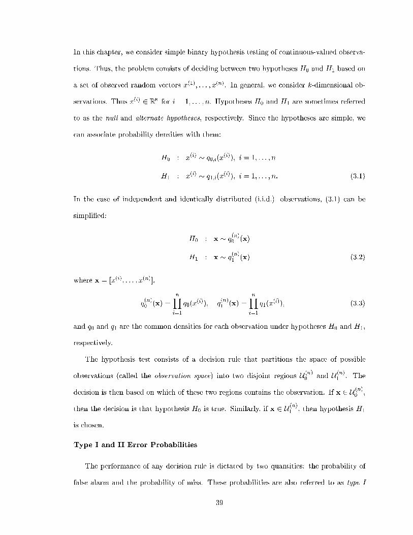
In this chapter, we consider simple binary hypothesis testing of continuous-valued observa-
tions. Thus, the problem consists of deciding between two hypotheses H0 and H1 based on
a set of observed random vectors x(1); : : : ; x(n). In general, we consider k-dimensional ob-
servations. Thus x(i) 2 Rk for i = 1; : : : ; n. Hypotheses H0 and H1 are sometimes referred
to as the null and alternate hypotheses, respectively. Since the hypotheses are simple, we
can associate probability densities with them:
H0 : x(i) � q0;i(x(i)); i = 1; : : : ; n
H1 : x(i) � q1;i(x(i)); i = 1; : : : ; n: (3.1)
In the case of independent and identically distributed (i.i.d.) observations, (3.1) can be
simpli�ed:
H0 : x � q(n)0 (x)
H1 : x � q(n)1 (x) (3.2)
where x = [x(i); : : : ; x(n)],
q(n)0 (x) =
nYi=1
q0(x(i)); q
(n)1 (x) =
nYi=1
q1(x(i)); (3.3)
and q0 and q1 are the common densities for each observation under hypotheses H0 and H1,
respectively.
The hypothesis test consists of a decision rule that partitions the space of possible
observations (called the observation space) into two disjoint regions U (n)0 and U (n)
1 . The
decision is then based on which of these two regions contains the observation. If x 2 U (n)0 ,
then the decision is that hypothesis H0 is true. Similarly, if x 2 U (n)1 , then hypothesis H1
is chosen.
Type I and II Error Probabilities
The performance of any decision rule is dictated by two quantities: the probability of
false alarm and the probability of miss. These probabilities are also referred to as type I
39

and type II probabilities of error, respectively. A type I error occurs when the decision is H1
and hypothesis H0 is true. Similarly, a type II error corresponds to a decision of H0 when
hypothesis H1 is true. Let � denote the probability of false alarm and � the probability of
miss. Then
� = P (Decide H1jH0 is true) =
ZU(n)1
q0(x)dx
� = P (Decide H0jH1 is true) =
ZU(n)0
q1(x)dx: (3.4)
Bayes Test
If the probabilities of the two hypotheses (known as prior probabilities, or simply priors)
are known, then a decision rule, known as a Bayes test, can be derived that minimizes a
criterion known as Bayes risk [69]. A special case of the Bayes risk is the probability of
error, or the probability of making an incorrect decision. To state this concretely, let the
null and alternate hypotheses be, respectively
H0 : x � q0
H1 : x � q1 (3.5)
and let the priors be
P0 = P (H0 is true)
P1 = P (H1 is true):
The probability of error given by
Pe = �P0 + �P1 (3.6)
is minimized by the Bayes test [69]:
q0(x)
q1(x)
H0
><H1
P1P0: (3.7)
40

Neyman-Pearson Test
In many cases, the prior probabilities are unknown and thus the Bayes test (3.7) can
not be derived. In such cases, the Neyman-Pearson theorem and the receiver operating
characteristic, described below, o�er assistance in determining optimal decision rules.
For the hypotheses given by (3.5), the well-known Neyman-Pearson Theorem [10, 39,
48, 69] states that under the constraint � � ��, the minimum � is achieved by a likelihood
ratio or log-likelihood ratio test:
�(x) = logq0(x)
q1(x)
H0
><H1
T: (3.8)
The threshold T will depend on the maximum allowable probability of miss ��. The
Neyman-Pearson theorem also states that under a constraint on false alarm probability
� � ��, the minimum � is achieved by the log-likelihood ratio test (3.8). Note that the
Neyman-Pearson test (3.8) is equivalent to a Bayes test for some particular values of the
priors. Speci�cally, if log(P1=P0) = T , then the Neyman-Pearson test is a Bayes test.
However, the utility of the Neyman-Pearson theorem is exhibited most when the priors are
unknown.
Note that in the case of n i.i.d. observations, the Neyman-Pearson test becomes
1
n
nXi=1
�(x(i))H0
><H1
T (3.9)
where the log-likelihood ratio is written in normalized form.
Receiver Operating Characteristic
A powerful illustrative tool for understanding hypothesis testing performance is the
receiver operating characteristic (ROC) curve [9, 55, 69]. For a given decision rule, many
pairs (�; �) of type I and type II error probabilities are achievable. The speci�c values of
� and � depend on some parameter of the rule. For Neyman-Pearson tests, this parameter
is the decision threshold T . Clearly, it is desirable to minimize both � and �, but in
general there is a tradeo� between these two quantities. The ROC curve provides a visual
41

interpretation of this tradeo�. The ROC curve is a graph of the probability of detection
1��, also known as the power of the test, versus the probability of false alarm � for a given
decision rule. For Neyman-Pearson tests, this graph is plotted parametrically as � and �
are both functions of the threshold T .
Optimality Criteria for Hypothesis Tests
There are several criteria by which a decision rule may be considered optimal. Two of
the most commonly used criteria are explained here. Interestingly, the Neyman-Pearson
theorem shows that likelihood ratio tests are optimal with respect to both criteria.
Often hypothesis tests are designed so that the probability of miss is minimized subject
to the constraint that the probability of false alarm does not exceed a pre-speci�ed maximum
tolerable value [55, 69]. That is: minimize the function �(�) on the set f� 2 (0; 1) : � � ��g.
The Neyman-Pearson theorem indicates that for this criterion, the optimal decision rule is
a likelihood or log-likelihood ratio test. The speci�c threshold that satis�es the false alarm
constraint while minimizing the probability of miss is not given by the theorem, but can
usually be determined numerically or analytically [10].
Another optimality criterion for a hypothesis test is the area under the ROC curve. Note
that this is actually an optimality criterion for a family of hypothesis tests, since each test
corresponds to only one point on the ROC curve. This criterion is similar to the previous
criterion in an \average" sense, since the objective is now to minimize the integral
Z 1
0�(�)d�:
Further motivation for selection of the area under the ROC curve as an optimality criterion
comes from the fact that when the likelihood ratio is Gaussian, the area is monotonically
related to the signal-to-noise ratio (SNR) by [3]
Area =1
2+1
2erf
�SNR
2
�
42

where the SNR is de�ned as [4]
SNR =(E[�jH0]�E[�jH1])
2
12(var[�jH0] + var[�jH1])
:
It can be shown that, like the previous criterion, the Neyman-Pearson test provides the
optimal decision rule [4]. This fact follows directly from the Neyman-Pearson theorem.
Discrimination and Stein's Lemma
The discrimination (also known as information discrimination, relative entropy, Kullback-
Leibler distance, and divergence) [10, 21] between two discrete sources with probability mass
functions (pmf's) qa(x) and qb(x) is de�ned as
L(qakqb) =Xi
qa(xi) logqa(xi)
qb(xi): (3.10)
Similarly, the discrimination between two continuous sources with densities qa(x) and qb(x)
is de�ned as
L(qakqb) =Zqa(x) log
qa(x)
qb(x)dx: (3.11)
Throughout this chapter, we assume that all logarithms are natural logarithms, unless
otherwise noted. The discriminations de�ned in (3.10) and (3.11) are thus given in nats.
The discrimination function �nds use in many areas of information theory. Worth noting
is the fact that discrimination is never negative [10, 21]. Its importance in simple binary
hypothesis testing is evidenced by Stein's lemma. This lemma states that for the hypotheses
given by (3.2) and (3.3), if the probability of false alarm is constrained to be less than or
equal to ��, then the minimum probability of miss ��n, over all decision rules with n i.i.d.
observations, satis�es [10]
limn!+1
(��n)1=n = e�L(q0kq1): (3.12)
Stein's lemma indicates that for the simple binary hypothesis testing problem, the discrim-
ination between the two source densities is an important measure of performance as the
43

number of observations increases. The lemma states that for any � 2 (0; 1), the mini-
mum possible � is an exponentially decreasing function of L(q0kq1). Another version of the
lemma shows that for any � 2 (0; 1), the minimum possible � is exponentially decreasing
in L(q1kq0).
Error Exponents and the Tilted Density
The asymptotic values of both the type I and II error probabilities as functions of the
Neyman-Pearson threshold can be obtained by using large deviations arguments and Sanov's
theorem [10, 12]. The essential result is that for simple binary hypotheses with n i.i.d.
observations, the probability of false alarm � and the probability of miss � are both expo-
nentially decreasing functions of discriminations. These discriminations, however, involve a
third density known as the tilted density [10]. To state this result concretely, consider the
hypotheses given by (3.2) and (3.3) and the Neyman-Pearson test (3.9). The tilted density
given in [10] is
q�(x) =q0(x)
1��q1(x)�R
q0(y)1��q1(y)�dy(3.13)
where � 2 [0; 1] is de�ned implicitly in terms of the threshold T of the Neyman-Pearson
test (3.9):
T =
Zq�(x) log
q0(x)
q1(x)dx = L(q�kq1)� L(q�kq0): (3.14)
Then from Sanov's theorem, it can be shown that [10]
e�nL(q�kq0)�o(n) � � � e�nL(q�kq0)
e�nL(q�kq1)�o(n) � � � e�nL(q�kq1):
Thus, for large n
� � e�nL(q�kq0)
� � e�nL(q�kq1): (3.15)
44

Note that in the Neyman-Pearson test (3.9), the threshold T may take any value in
R, but as � 2 [0; 1] is varied in the de�nition (3.14) of T , we see that �L(q1kq0) � T �
L(q0kq1). However, as n ! +1, by the weak law of large numbers, the normalized log-
likelihood ratio is with high probability close to its conditional mean under hypothesis H0
or H1. The conditional means under H0 and H1 are L(q0kq1) and �L(q1kq0), respectively.
Consequently, thresholds outside the range [�L(q1kq0); L(q0kq1)] correspond to regions on
the ROC curve where � � 0 or � � 0. The set of thresholds within this range maps to the
entire ROC curve as n! +1.
The formulas (3.15) indicate that for a given value of the threshold T , the discriminations
L(q�kq0) and L(q�kq1) are crucial in determining the performance of the Neyman-Pearson
test. In Section 3.6.3, we shall utilize this fact for vector quantizer design.
Cherno� Information
The asymptotic behavior of the total probability of error in a Bayes test can be deter-
mined using Cherno�'s theorem [21]. This theorem states that for n large, the probability
of error in the Bayes test (3.7) is exponentially decreasing in n and the greatest possible
exponent in the probability of error is
C(q0; q1) = L(q��kq0) = L(q��kq1) (3.16)
where �� is chosen such that the two discriminations L(q��kq0) and L(q��kq1) are equal.
The quantity C(q0; q1) in (3.16) is called the Cherno� information.
3.2.2 Vector Quantization
Vector quantization [26, 27, 30, 46, 60, 75, 76] is an e�ective source coding technique
for random vectors. Like a scalar quantizer, a vector quantizer consists of a set of cells and
codebook points. Unlike a scalar quantizer, whose set of cells consists of intervals or unions
of intervals, a vector quantizer's cells are regions in multidimensional Euclidean space. The
advantage of vector quantization over scalar quantization is the ability to achieve non-
45

rectangular cell shapes. Often this results in improved performance, usually measured by
mean square error.
Mathematical Description
A vector quantizer [27, 46] (VQ) Q = (S; C) consists of a codebook C = fx1; : : : ; xNg
and a set of cells S = fS1; : : : ; SNg that partition Rk . For each i, the codebook point xi
lies in cell Si. The VQ operator can be written as
Q(x) = xi; for x 2 Si
where the input x 2 Rk and the VQ is said to be k-dimensional. For a vector quantizer
Q, let Vi =RSidx denote the volume of the ith cell. The speci�c point density [46] of Q is
de�ned as
�s(x) =1
NVi; for x 2 Si:
For large N , as its name suggests, this function is a density of points. When integrated
over a small region A, it gives the approximate fraction of codebook points contained in A.
Next, de�ne the diameter function of the VQ as
d(x) = supfku� vk : u; v 2 Sig; for x 2 Si:
The (scalar) speci�c inertial pro�le function ms(x) is de�ned as [26]
ms(x) =
RSiky � xik2dyV1+2=ki
; for x 2 Si: (3.17)
Note that ms(x) is invariant to a scaling of Si. This function contains information about
the shapes of the cells of the VQ. Similarly, we de�ne the following matrix function Ms(x)
called the speci�c covariation pro�le
Ms(x) =
RSi(y � xi)(y � xi)
T dy
V1+2=ki
; for x 2 Si:
This function is also scale invariant.
46

Role of Vector Quantization in Communication Systems
In a communication system, a message must be transmitted from one location to another
across a channel that usually causes degradation of the transmitted signal. The objective of
the communication system designer is to transmit the message with minimal degradation
and at the maximum data rate [59].
In his seminal 1948 paper [61], Shannon showed that, through channel coding, a channel
may be considered errorless when the rate of the transmitted data does not exceed a thresh-
old known as channel capacity. However, meeting this rate constraint usually requires lossy
compression of the message, especially when the message is continuously distributed.
Compression, or source coding, is therefore an important step in the transmission pro-
cess. The rate of a source encoder, de�ned to be the average number of bits output per
input sample, must be made as low as possible so that transmission above channel capacity
is not attempted, and so that transmission is carried out eÆciently. The rate of a vector
quantizer is log2N where N is the number of quantizer cells. A good quantizer has both a
small rate and high �delity, or quality of the decoded message. High �delity is equivalent
to low distortion. Vector quantization is a powerful source coding technique for both uni-
variate and multivariate sources. In the following section, we describe the most common
measure of distortion for VQ design. Then, in the remainder of the chapter, we formulate
the theory for distortion measures that can be used to design VQ's that are optimal for
hypothesis testing.
Estimation-Optimal Vector Quantization
Much of the research done on vector quantization has focused on the rth-power distortion
[46] given by
D =1
kE [kx�Q(x)kr]
=1
k
Zkx�Q(x)krq(x)dx
47

where q(x) is the probability density of the source. If we set r = 2 and use D � k as the
distortion measure, we get the commonly-used mean square reconstruction error (MSE):
MSE = E�kx�Q(x)k2� :
Since reconstruction MSE is a widely-used distortion measure for estimators [55], we refer
to minimum MSE quantizers as estimation-optimal quantizers.
The asymptotic (in N) rth-power distortion of a many-point VQ has been determined
in [46]. To determine this value, a \sequence approach" was taken, in which a sequence of
quantizers fQNg was considered. Each quantizer in the sequence was characterized by its
speci�c point density and speci�c inertial pro�le.1 Then, assuming that the sequences of
speci�c point densities and speci�c inertial pro�les converge to functions �(x) and m(x),
called the point density and inertial pro�le, respectively, and assuming the sequence of
diameter functions converges to zero, it is shown that
limN!+1
N2=kE�kx�QN (x)k2
�=
Zq(x)m(x)
�(x)2=kdx: (3.18)
Equation (3.18), known as Bennet's integral, gives an approximation to the MSE of a many-
point VQ. For a given inertial pro�le, the point density that minimizes Bennet's integral,
obtained by H�older's inequality or calculus of variations, is given by [43, 47]
�(x) =[q(x)m(x)]
kk+2R
[q(y)m(y)]k
k+2dy:
Using this in (3.18) gives
MSE � 1
N2=k
�Z[q(x)m(x)]
kk+2dx
� k+2k
:
A conjecture by Gersho [26], believed by many to be true, states that many-point VQ's
that are optimal with respect to rth-power distortion have cells that are approximately
congruent. Furthermore, the moment of inertia of the congruent cells is the minimum
moment of inertia m�s;k of all cells that tessellate in Rk . A quantizer with congruent cells
1Note that the speci�c inertial pro�le in [46] di�ers slightly from our de�nition.
48

has a constant inertial pro�le and, as a result, the estimation-optimal point density is given
by [26, 46]
�e(x) =q(x)
kk+2R
q(y)k
k+2dy: (3.19)
The MSE of an N -point, k-dimensional VQ can then be upper bounded by the so-called
Zador-Gersho formula [26, 75]:
MSE /m�
s;k
N2=k
�Zq(x)
kk+2dx
� k+2k
: (3.20)
The covariation pro�le (the limit of the sequence of speci�c covariation pro�les) of the
estimation-optimal quantizer is also constant, as the cells are congruent, and is equal to a
multiple of the identity matrix. This follows from a theorem by Zamir and Feder [77] that
states that the components of the error vector of an optimal lattice quantizer (a quantizer
for which each cell is a translation of a basic cell) are uncorrelated.
Bennet's integral is well suited to the analysis of the estimation performance of struc-
tured quantizers. In [46] it is shown that the (estimation) performance loss of a suboptimal
quantizer, de�ned as the ratio of the quantizer's distortion (MSE) to that of the optimal
quantizer with the same rate, can be factored into the product of two individual losses
called the point density loss and the cell shape loss. As their names suggest, these losses are
attributable to the suboptimality of the quantizer's point density and inertial pro�le (cell
shapes), respectively.
3.3 Lossless Quantizers for Distributed Hypothesis Testing
In the remainder of this chapter, we develop procedures for designing vector quantizers
that are optimal for the distributed hypothesis testing problem illustrated in Figure 3.1.
We focus on the case of i.i.d. observations x(1); : : : ; x(n), but point out that the analysis can
be extended to independent, non-identical observations as well. Our goal is to design the
quantizers Q1; : : : ; Qn in Figure 3.1 so that the performance of the hypothesis test utilizing
the n quantized observations is maximized. Unless otherwise stated, we assume that the
49
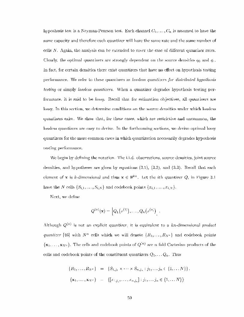
hypothesis test is a Neyman-Pearson test. Each channel C1; : : : ; Cn is assumed to have the
same capacity and therefore each quantizer will have the same rate and the same number of
cells N . Again, the analysis can be extended to cover the case of di�erent quantizer rates.
Clearly, the optimal quantizers are strongly dependent on the source densities q0 and q1.
In fact, for certain densities there exist quantizers that have no e�ect on hypothesis testing
performance. We refer to these quantizers as lossless quantizers for distributed hypothesis
testing or simply lossless quantizers. When a quantizer degrades hypothesis testing per-
formance, it is said to be lossy. Recall that for estimation objectives, all quantizers are
lossy. In this section, we determine conditions on the source densities under which lossless
quantizers exist. We show that, for these cases, which are restrictive and uncommon, the
lossless quantizers are easy to derive. In the forthcoming sections, we derive optimal lossy
quantizers for the more common cases in which quantization necessarily degrades hypothesis
testing performance.
We begin by de�ning the notation. The i.i.d. observations, source densities, joint source
densities, and hypotheses are given by equations (3.1), (3.2), and (3.3). Recall that each
element of x is k-dimensional and thus x 2 Rkn . Let the ith quantizer Qi in Figure 3.1
have the N cells fSi;1; : : : ; Si;Ng and codebook points fxi;1; : : : ; xi;Ng.
Next, we de�ne
Q(n)(x) =hQ1
�x(1)
�; : : : ; Qn
�x(n)
�i:
Although Q(n) is not an explicit quantizer, it is equivalent to a kn-dimensional product
quantizer [46] with Nn cells which we will denote fR1; : : : ; RNng and codebook points
fx1; : : : ;xNng. The cells and codebook points of Q(n) are n-fold Cartesian products of the
cells and codebook points of the constituent quantizers Q1; : : : Qn. Thus
fR1; : : : ; RNng = fS1;j1 � � � � � Sn;jn : j1; : : : jn 2 f1; : : : Ngg ;
fx1; : : : ;xNng = f[x1;j1 ; : : : ; xn;jn ] : j1; : : : jn 2 f1; : : : Ngg
50

and the product quantizer codebook point [x1;j1 ; : : : ; xn;jn ] lies in the cell given by S1;j1 �
� � � � Sn;jn.
The probability mass functions of the observation x(i) after quantization by the quantizer
Qi, under hypotheses H0 and H1, are given by
�q0;Qi;j =
ZSi;j
q0(x)dx
�q1;Qi;j =
ZSi;j
q1(x)dx (3.21)
for j 2 f1; : : : ; Ng. Note that since x(1); : : : ; x(n) are i.i.d., the quantized observations are
also independent, though not necessarily identically distributed. The joint probability mass
functions of the quantized observation Q(n)(x) are
�q(n)0 ([x1;j1 ; : : : ; xn;jn ]) =
nYi=1
�q0;Qi;ji
�q(n)1 ([x1;j1 ; : : : ; xn;jn ]) =
nYi=1
�q1;Qi;ji : (3.22)
The probabilities of type I and II errors of a Neyman-Pearson test using the quantized
observation Q(n)(x) are partial sums of the pmf's in (3.22). From (3.21), it is clear that
these error probabilities are independent of the codebooks of quantizers Q1; : : : ; Qn. From
(3.10), the discriminations between the marginal and joint pmf's of the quantized sources,
under the two hypotheses, are also independent of the quantizers' codebooks. Thus, the
quantizers may be characterized solely by their partitions, or cells.
The following theorem shows that for certain hypothesis testing objectives with i.i.d.
observations, the optimal quantizers Q1; : : : ; Qn must have identical cells. This allows us to
restrict our attention to the design of a single quantizer. We then derive conditions under
which this single quantizer is lossless.
Theorem 3.1 Let the observations x(1); : : : ; x(n) be i.i.d. under each hypothesis. If the
quantizers Q1; : : : ; Qn maximize the discrimination L��q(n)0 k�q(n)1
�, then their cells are equiv-
alent.
51

Proof: Since the observations are independent, the discrimination between the joint
pmf's is the sum of the individual discriminations [10]:
L��q(n)0
�q(n)1
�=
nXi=1
L(�q0;Qik�q1;Qi
)
where �q0;Qiand �q1;Qi
are the pmf's of Qi(x(i)), whose probabilities are given by (3.21). Now
suppose the quantizers Q1; : : : ; Qn maximize L��q(n)0 k�q(n)1
�. Then, for each i 2 f1; : : : ; ng,
the discrimination L(�q0;Qik�q1;Qi
) must be maximized by the ith quantizer Qi. This discrim-
ination is a function of the marginal densities q0 and q1 as well as the ith quantizer's cells.
Therefore, each quantizer must have the same cells. 2
Identical-partition quantizers are also optimal for asymptotic probability of false alarm
or miss. To prove this, we must �rst extend the relations (3.15) to the case of independent,
non-identical observations. Doing so gives the following asymptotic equations for � and �,
the probabilities of type I and II errors with n quantized observationsQ1
�x(1)
�; : : : ; Qn
�x(n)
�:
log � � �nXi=1
L(q�;Qik�q0;Qi
)
log � � �nXi=1
L(q�;Qik�q1;Qi
)
where q�;Qiis the tilted mass function associated with �q0;Qi
and �q1;Qi(see Section 3.5.1 and
equation (3.32)). By arguments similar to those in the proof of Theorem 3.1, we conclude
that quantizers that are optimal with respect to � or � have identical cells.
We now focus on quantizers Q1; : : : ; Qn with identical cells. Further, since a quantizer's
codebook does not a�ect hypothesis testing performance, we assume the quantizers have
identical codebooks as well. Thus, the quantizers are identical and will be denoted Q. The
product quantizer Q(n) then consists of n identical constituent quantizers Q and
Q(n)(x) =hQ�x(1)
�; : : : ; Q
�x(n)
�i:
52
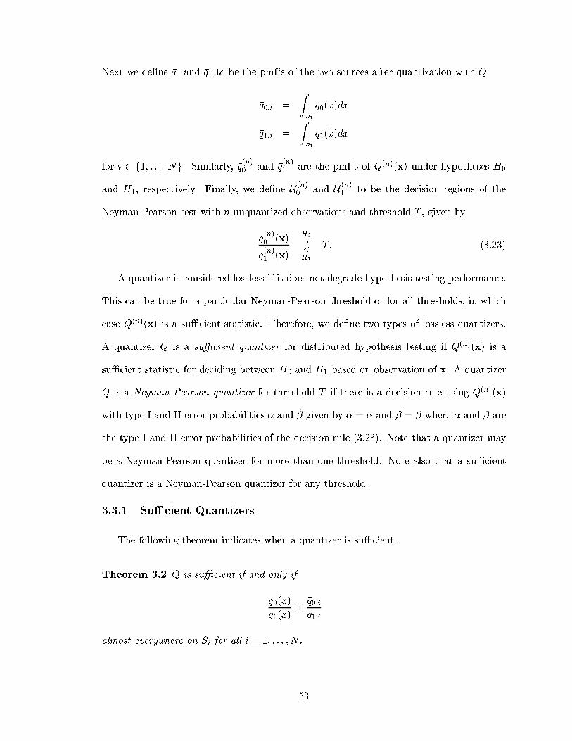
Next we de�ne �q0 and �q1 to be the pmf's of the two sources after quantization with Q:
�q0;i =
ZSi
q0(x)dx
�q1;i =
ZSi
q1(x)dx
for i 2 f1; : : : ; Ng. Similarly, �q(n)0 and �q
(n)1 are the pmf's of Q(n)(x) under hypotheses H0
and H1, respectively. Finally, we de�ne U (n)0 and U (n)
1 to be the decision regions of the
Neyman-Pearson test with n unquantized observations and threshold T , given by
q(n)0 (x)
q(n)1 (x)
H0
><H1
T: (3.23)
A quantizer is considered lossless if it does not degrade hypothesis testing performance.
This can be true for a particular Neyman-Pearson threshold or for all thresholds, in which
case Q(n)(x) is a suÆcient statistic. Therefore, we de�ne two types of lossless quantizers.
A quantizer Q is a suÆcient quantizer for distributed hypothesis testing if Q(n)(x) is a
suÆcient statistic for deciding between H0 and H1 based on observation of x. A quantizer
Q is a Neyman-Pearson quantizer for threshold T if there is a decision rule using Q(n)(x)
with type I and II error probabilities � and � given by � = � and � = � where � and � are
the type I and II error probabilities of the decision rule (3.23). Note that a quantizer may
be a Neyman-Pearson quantizer for more than one threshold. Note also that a suÆcient
quantizer is a Neyman-Pearson quantizer for any threshold.
3.3.1 SuÆcient Quantizers
The following theorem indicates when a quantizer is suÆcient.
Theorem 3.2 Q is suÆcient if and only if
q0(x)
q1(x)=
�q0;i�q1;i
almost everywhere on Si for all i = 1; : : : ; N .
53

Proof: The statistic Q(n)(x) is suÆcient for deciding between H0 and H1 based on
observation of x if and only if [10]
L�q(n)0
q(n)1
�= L
��q(n)0
�q(n)1
�:
Since the observations x(1); : : : ; x(n) are i.i.d., this is equivalent to
L(q0kq1) = L(�q0k�q1):
The discrimination between the sources q0 and q1 is
L(q0kq1) =
Zq0(x) log
q0(x)
q1(x)dx
=
NXi=1
ZSi
q0(x) logq0(x)
q1(x)dx:
The discrimination between the quantized sources �q0 and �q1 is
L(�q0k�q1) =
NXi=1
�q0;i log�q0;i�q1;i
:
The loss in discrimination due to quantization is
L(q0kq1)� L(�q0k�q1) =NXi=1
ZSi
q0(x) logq0(x)�q1;iq1(x)�q0;i
dx
�NXi=1
ZSi
q0(x)
�1� q1(x)�q0;i
q0(x)�q1;i
�dx
= 1�NXi=1
�q0;i�q1;i
ZSi
q1(x)dx
= 0: (3.24)
The inequality in the second step of (3.24) derives from log(1=a) � 1�a. Thus the inequality
L(q0kq1) � L(�q0k�q1) holds with equality if and only if
q1(x)�q0;iq0(x)�q1;i
= 1
almost everywhere on Si for all i = 1; : : : ; N , which proves the theorem. 2
Theorem 3.2 gives a condition on the quantizer cells that ensures suÆciency. The next
theorem gives a condition on the source densities that ensures the existence of a suÆcient
quantizer.
54

Theorem 3.3 A suÆcient quantizer exists if and only if the likelihood ratio q0(x)=q1(x) is
piecewise-constant almost everywhere on Rk .
Proof: Suppose the likelihood ratio is piecewise constant almost everywhere. Then we
can write
q0(x)
q1(x)=
KXi=1
aiIAi(x) + z(x)
where fA1; : : : ; AKg is a set of disjoint, exhaustive, and connected regions in Rk , ai 2 R
for all i = 1; : : : ;K, IU (x) is the indicator function of the set U , and z(x) is zero almost
everywhere. 2
Let the quantizer Q have N = K cells fS1; : : : ; SNg where Si = Ai for all i. Now,
q0(x)=q1(x) = ai almost everywhere on Si. Therefore
�q0;i�q1;i
=
RSiq0(y)dyR
Siq1(y)dy
=
RSiaiq1(y)dyR
Siq1(y)dy
= ai:
Thus
�q0;i�q1;i
=q0(x)
q1(x)
almost everywhere on Si. By Theorem 3.2, Q is suÆcient.
Next, let l(x) be the likelihood ratio and suppose l(x) is not piecewise-constant almost
everywhere. Then for an N -point quantizer with N < +1, there is a cell Si such that l(x)
is not constant almost everywhere on Si. From Theorem 3.2, the quantizer is not suÆcient.
2
Note that Theorem 3.3 is equivalent to stating that a suÆcient quantizer exists if and
only if the joint likelihood ratio can be written in the form
q(n)0 (x)
q(n)1 (x)
=nY
j=1
NXi=1
aiIAi
�x(j)�+ z(x)
where z(x) is zero almost everywhere on Rkn .
2We take this to be the de�nition of piecewise-constant almost everywhere.
55

3.3.2 Neyman-Pearson Quantizers
The previous section gave a condition on the quantizer's cells that guaranteed suÆciency
and a condition on the sources that ensured existence of a suÆcient quantizer. In this
section, we prove similar theorems for Neyman-Pearson quantizers. The �rst theorem states
that each cell of the product quantizer Q(n) associated with a Neyman-Pearson quantizer
Q is contained in one of the Neyman-Pearson regions U (n)0 or U (n)
1 .
Theorem 3.4 A quantizer Q is a Neyman-Pearson quantizer for threshold T if and only
if for every cell Ri of Q(n) with P (RijH0) > 0 and P (RijH1) > 0, V
�Ri \ U (n)
0
�= 0 or
V�Ri \ U (n)
1
�= 0 where V (U) is the volume of the set U .
Proof: First assume the conditions of the theorem hold. We note that T > 0, U (n)0 =
fx : q(n)0 (x) > Tq
(n)1 (x)g, and U (n)
1 = fx : q(n)0 (x) < Tq
(n)1 (x)g. If P (RijH0) = 0, then
q(n)0 (x) = 0 a.e. on Ri and, therefore, V
�Ri \ U (n)
0
�= 0. Similarly, if P (RijH1) = 0, then
V�Ri \ U (n)
1
�= 0. Thus, for each cell Ri with non-zero probability under at least one
hypothesis, one of the volumes is zero.
Now de�ne the following decision rule based on observation of Q(n)(x) = xi:
V�Ri \ U (n)
0
� H0
><H1
V�Ri \ U (n)
1
�: (3.25)
This rule can be implemented in a more straightforward manner if the codebook is selected
properly. Later, we will see that this is actually a Neyman-Pearson test on the quantized
data. Recall that for any i, one of the volumes in (3.25) must be zero.
The probability of false alarm with this decision rule is
� =X
fi:V (Ri\U(n)0 )=0g
�q(n)0 (xi) =
Xfi:V (Ri\U
(n)0 )=0g
ZRi
q(n)0 (x)dx =
ZU(n)1
q(n)0 (x)dx = �
where � is the probability of false alarm of the Neyman-Pearson decision rule with unquan-
tized data (3.23). It can be similarly shown that the probability of miss is unchanged as well.
Thus, Q is a Neyman-Pearson quantizer for threshold T , and (3.25) is a Neyman-Pearson
test.
56
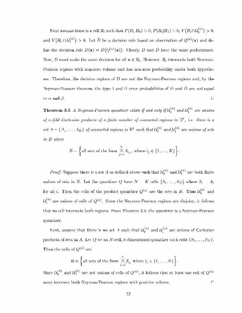
Next assume there is a cell Ri such that P (RijH0) > 0, P (RijH1) > 0, V�Ri\U (n)
0
�> 0,
and V�Ri \ U (n)
1
�> 0. Let D be a decision rule based on observation of Q(n)(x) and de-
�ne the decision rule D(x) = D�Q(n)(x)
�. Clearly D and D have the same performance.
Now, D must make the same decision for all x 2 Ri. However, Ri intersects both Neyman-
Pearson regions with non-zero volume and has non-zero probability under both hypothe-
ses. Therefore, the decision regions of D are not the Neyman-Pearson regions and, by the
Neyman-Pearson theorem, the type I and II error probabilities of D and D are not equal
to � and �. 2
Theorem 3.5 A Neyman-Pearson quantizer exists if and only if U (n)0 and U (n)
1 are unions
of n-fold Cartesian products of a �nite number of connected regions in Rk , i.e. there is a
set A = fA1; : : : ; AKg of connected regions in Rk such that U (n)0 and U (n)
1 are unions of sets
in B where
B =
�all sets of the form
n
�j=1
Aij ; where ij 2 f1; : : : ;Kg�:
Proof: Suppose there is a set A as de�ned above such that U (n)0 and U (n)
1 are both �nite
unions of sets in B. Let the quantizer Q have N = K cells fS1; : : : ; SNg where Si = Ai
for all i. Then the cells of the product quantizer Q(n) are the sets in B. Thus U (n)0 and
U (n)1 are unions of cells of Q(n). Since the Neyman-Pearson regions are disjoint, it follows
that no cell intersects both regions. From Theorem 3.4, the quantizer is a Neyman-Pearson
quantizer.
Next, assume that there is no set A such that U (n)0 and U (n)
1 are unions of Cartesian
products of sets in A. Let Q be an N -cell, k-dimensional quantizer with cells fS1; : : : ; SNg.
Then the cells of Q(n) are
R =
�all sets of the form
n
�j=1
Sij where ij 2 f1; : : : ; Ng�:
Since U (n)0 and U (n)
1 are not unions of cells of Q(n), it follows that at least one cell of Q(n)
must intersect both Neyman-Pearson regions with positive volume. 2
57

3.3.3 Examples of Lossless Quantizers
We now give some examples of sources for which lossless quantizers exist. First we show
that for n = 1, a Neyman-Pearson quantizer always exists. For n > 1, however, lossless
quantizers usually do not exist.
Non-Distributed Hypothesis Testing
When the observation x comes from a single source (n = 1), a Neyman-Pearson quantizer
always exists. Thus, for the non-distributed hypothesis testing scenario, it is possible to
design a quantizer for which no performance loss is incurred. Furthermore, in some cases
this quantizer can have a rate of only one bit.
To prove this, we �rst note that for n = 1, the Neyman-Pearson regions U (n)0 and U (n)
1
for threshold T are subsets of Rk . Assume each of these regions is connected. Then clearly
the conditions of Theorem 3.5 are satis�ed with A =�U (n)
0 ;U (n)1
and n = 1. Next, let
the quantizer Q = Q(n) have cells U (n)0 and U (n)
1 . By Theorem 3.4, Q is a Neyman-Pearson
quantizer for threshold T . Since Q has only two cells, its rate is one bit. This formulation
can easily be extended to the case of non-connected Neyman-Pearson regions. In such cases,
a Neyman-Pearson quantizer must have more than two cells.
Next, suppose a quantizer is a Neyman-Pearson quantizer for K di�erent thresholds for
n = 1. Then there are up to K pairs of type I and II error probabilities that are una�ected
by the quantizer. Therefore, the ROC curve of the Neyman-Pearson test with quantized
data will intersect that of the unquantized curve in up to K places as shown in Figure 3.2.
Suppose now that we have n = 2 observations and two quantizers. In most cases, when
n > 1 Neyman-Pearson quantizers do not exist. Thus the quantized ROC curve will not
intersect the unquantized curve. This is also illustrated in Figure 3.2.
58
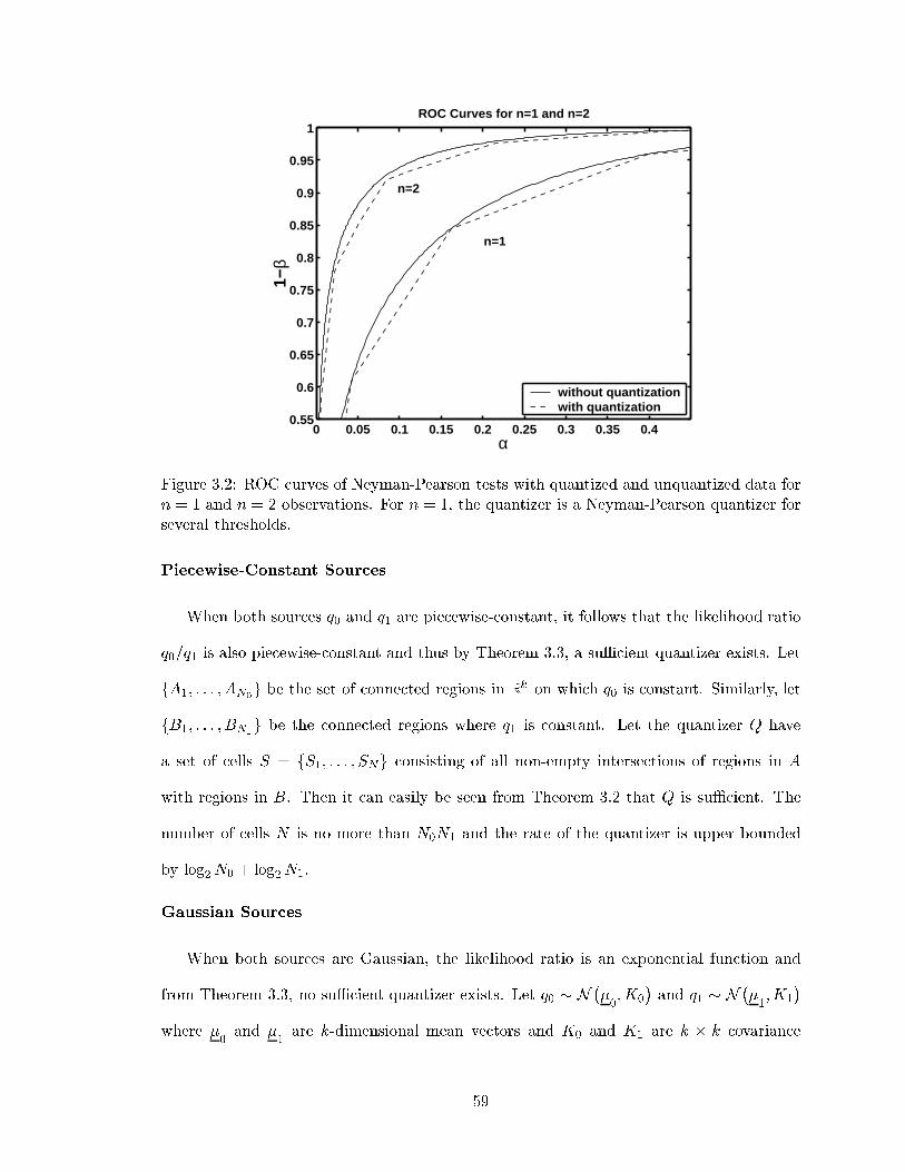
0 0.05 0.1 0.15 0.2 0.25 0.3 0.35 0.40.55
0.6
0.65
0.7
0.75
0.8
0.85
0.9
0.95
1
α
1−β
ROC Curves for n=1 and n=2
n=1
n=2
without quantizationwith quantization
Figure 3.2: ROC curves of Neyman-Pearson tests with quantized and unquantized data forn = 1 and n = 2 observations. For n = 1, the quantizer is a Neyman-Pearson quantizer forseveral thresholds.
Piecewise-Constant Sources
When both sources q0 and q1 are piecewise-constant, it follows that the likelihood ratio
q0=q1 is also piecewise-constant and thus by Theorem 3.3, a suÆcient quantizer exists. Let
fA1; : : : ; AN0g be the set of connected regions in Rk on which q0 is constant. Similarly, let
fB1; : : : ; BN1g be the connected regions where q1 is constant. Let the quantizer Q have
a set of cells S = fS1; : : : ; SNg consisting of all non-empty intersections of regions in A
with regions in B. Then it can easily be seen from Theorem 3.2 that Q is suÆcient. The
number of cells N is no more than N0N1 and the rate of the quantizer is upper bounded
by log2N0 + log2N1.
Gaussian Sources
When both sources are Gaussian, the likelihood ratio is an exponential function and
from Theorem 3.3, no suÆcient quantizer exists. Let q0 � N ��0;K0
�and q1 � N ��
1;K1
�where �
0and �
1are k-dimensional mean vectors and K0 and K1 are k � k covariance
59

−5 0 5−5
−4
−3
−2
−1
0
1
2
3
4
5
x(1)
x(2)
Product Quantizer Cells and Neyman−Pearson Decision Regions
Figure 3.3: Border (dashed line) between Neyman-Pearson regions for Gaussian sources andcells of a two-dimensional product quantizer (solid lines).
matrices. The likelihood ratio is
q0(x)
q1(x)=
sjK1jjK0j exp
��1
2(x� �
0)TK�1
0 (x� �0)� 1
2(x� �
1)TK�1
1 (x� �1)
�:
Since this function is not piecewise-constant on Rk , no suÆcient quantizer exists. Further-
more, for any threshold T with n > 1, it can be shown that no Neyman-Pearson quantizer
exists.
For example, let q0 � N (��; 1), q1 � N (�; 1), and n = 2. Since the sources are one-
dimensional (k = 1), the cells of Q(n) are Cartesian products of intervals, or rectangles.
However, the Neyman-Pearson regions are
U (n)0 =
nx = [x(1); x(2)] : x(1) + x(2) > T 0
oU (n)1 =
nx = [x(1); x(2)] : x(1) + x(2) < T 0
o
where T 0 = � log T=2�. Thus the Neyman-Pearson regions are separated by a line of
slope �1 in the x(1); x(2) plane. Figure 3.3 shows the border between the Neyman-Pearson
regions for � = 2 and T = 1 along with the cells of a product quantizer Q(n). Note that
60

since the product quantizer must have rectangular cells, some cells must intersect both
Neyman-Pearson regions.
3.3.4 Estimation Performance of Lossless Quantizers
The derivations in this section have neglected any consideration of quantizer estimation
performance. Indeed, it is quite possible that a lossless quantizer can have very poor esti-
mation performance. For example, a two-cell Neyman-Pearson quantizer can be expected
to yield a large reconstruction MSE. To improve estimation performance, one could apply
the techniques of Gray et al. [29, 50, 53] who consider a Bayes risk weighted rth-power dis-
tortion measure. The weighting factor is used to trade detection performance for estimation
performance. The weighted distortion is minimized by an iterative descent algorithm.
Another method of improving estimation performance is to re�ne the lossless quantizer.
Let Q and Q0 be vector quantizers. The quantizer Q0 is a re�nement of Q if Q0 has more
cells than Q and every cell of Q0 is a subset of some cell of Q. Now, suppose Q is a
lossless quantizer with minimum rate and N cells. The estimation performance of Q can
be improved by re�ning Q. That is, a re�nement of Q with N 0 > N cells may be optimized
for estimation performance, perhaps by means of an iterative algorithm. The detection
performance will of course remain unchanged. Note that in optimizing the re�ned quantizer
for estimation performance, both the codebook and partition must be considered.
3.4 Lossy Quantizers for Distributed Hypothesis Testing
Theorems 3.3 and 3.5 indicate that lossless quantizers exist only under rather restrictive
circumstances. Most sources, including Gaussian sources, do not satisfy the conditions of
the theorems. For these sources, quantization always results in a degradation in hypothesis
testing performance. In the proceeding sections, we will be concerned with the design of
quantizers for these cases. Although there will always be a loss in performance, this loss
can be minimized by proper design of the quantizer.
61

-x�(x) - Q�
-
Figure 3.4: A log-likelihood ratio quantizer.
3.4.1 Sequences of Quantizers
Asymptotic, or high-rate quantization analysis is commonly used to obtain interesting
insights into the behavior of many-point quantizers. Bennet's integral [26, 46] is the product
of such analysis. The most commonly used technique of asymptotic analysis is the sequence
approach. This technique has been introduced in Section 3.2.2 and is described in detail in
Appendix E where it is used to derive asymptotic losses in discrimination due to quantiza-
tion. The idea behind the sequence approach is to consider a sequence of quantizers fQNg.
Each quantizer in the sequence has associated with it a speci�c point density, speci�c in-
ertial pro�le, speci�c covariation pro�le, and diameter function. Assuming the �rst three
sequences of functions converge to functions �(x), m(x), M(x), and that the sequence of
diameter functions converges to zero, the limiting behavior of the quantizer sequence can
be determined. The resulting formulas can then be used to approximate the behavior of a
many-point quantizer by assuming it is part of such a sequence.
3.4.2 Log-Likelihood Ratio Quantizers
The performance of Neyman-Pearson hypothesis tests is una�ected by processing of
the observations as long as the processing produces a suÆcient statistic. For example,
quantization with a suÆcient quantizer (if one exists) has no e�ect on hypothesis testing
performance. If a suÆcient quantizer does not exist, then it is reasonable to quantize a
suÆcient statistic, such as the log-likelihood ratio, rather than the raw data, as the required
rate may be less than for a quantizer applied to the raw data. It has been determined that
this approach is optimal for various detection-related objectives [54, 68]. A log-likelihood
62

ratio quantizer or LLR quantizer Q is a function given by
Q(x) = Q�(�(x)) (3.26)
where �(x) is the log-likelihood ratio. The scalar quantizer Q� is called the constituent
quantizer of Q. Figure 3.4 depicts schematically a log-likelihood ratio quantizer. Note
that a k-dimensional vector quantizer Q is equivalent to some LLR quantizer if and only
if �(x) : Rk ! R is a one-to-one correspondence. Note also that the boundaries of an
LLR quantizer correspond to subsets of Rk on which the log-likelihood ratio is constant
(level sets of �(x)). Finally, recall from Section 3.3 that the codebook of the quantizer is
inconsequential for hypothesis testing.
Let q�;0(l) and q�;1(l) be the probability densities of �(x) under hypotheses H0 and H1,
respectively. Consider a sequence of LLR quantizers fQNg where QN (x) = QN;�(�(x)) and
assume that the sequence of diameter functions associated with the constituent quantizers
QN;� converges to zero. Then by Bennet's integral, the mean square reconstruction error
of the quantized log-likelihood ratio under either hypothesis converges to zero:
E�(l �QN;�(l))
2jH0
�=
Zq�;0(l)(l �QN;�(l))
2dl ! 0
E�(l �QN;�(l))
2jH1
�=
Zq�;1(l)(l �QN;�(l))
2dl ! 0: (3.27)
From (3.27), it is evident that the sequence of quantized observations fQN (x)g converges
to the suÆcient statistic �(x) and therefore, the degradation in hypothesis testing perfor-
mance vanishes as N ! +1. Therefore, an LLR quantizer whose constituent quantizer has
small cells should provide good hypothesis testing performance. In Section 3.6.4, we discuss
optimization of the constituent quantizer. On the other hand, it is certainly possible that
the reconstruction MSE of the sequence fQNg does not converge to zero, especially when
�(x) is many-to-one. For example, if k = 2 and the sources are q0 � N ([�0; �0]; I) and
q1 � N ([�1; �1]; I), then the constituent quantizer will attempt to preserve the sum of the
components of the observation vector. Thus, the cells of the LLR quantizer will be \strips"
63
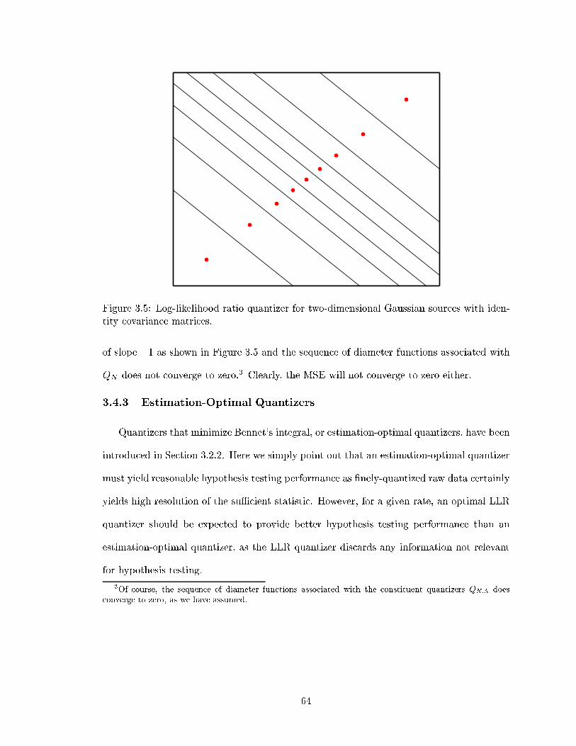
Figure 3.5: Log-likelihood ratio quantizer for two-dimensional Gaussian sources with iden-tity covariance matrices.
of slope �1 as shown in Figure 3.5 and the sequence of diameter functions associated with
QN does not converge to zero.3 Clearly, the MSE will not converge to zero either.
3.4.3 Estimation-Optimal Quantizers
Quantizers that minimize Bennet's integral, or estimation-optimal quantizers, have been
introduced in Section 3.2.2. Here we simply point out that an estimation-optimal quantizer
must yield reasonable hypothesis testing performance as �nely-quantized raw data certainly
yields high resolution of the suÆcient statistic. However, for a given rate, an optimal LLR
quantizer should be expected to provide better hypothesis testing performance than an
estimation-optimal quantizer, as the LLR quantizer discards any information not relevant
for hypothesis testing.
3Of course, the sequence of diameter functions associated with the constituent quantizers QN;� doesconverge to zero, as we have assumed.
64

3.4.4 Small-Cell Quantizers
A many-point quantizer for which most cells have small diameter can be considered to be
part of a sequence of quantizers whose diameter functions converge to zero. Such a quantizer
will be referred to as a small-cell quantizer. Bennet's integral (3.18) is obtained using the
sequence approach and is therefore only applicable to small-cell quantizers. An estimation-
optimal quantizer is a small-cell quantizer, whereas an LLR quantizer may or may not
be a small-cell quantizer. Note also that any small-cell quantizer should have reasonable
estimation performance, as the reconstruction MSE is proportional to N�2=k. In the next
section, we introduce quantizers that are optimized for hypothesis testing performance under
a small-cell constraint.
3.5 Asymptotic Analysis of Quantization for HypothesisTesting
In Section 3.2.1, the discriminations L(q0kq1), L(q1kq0), L(q�kq0), and L(q�kq1) were
shown to play an important role in the determination of hypothesis testing performance. In
general, a Neyman-Pearson hypothesis test performs better as these quantities are increased.
In this section, we analyze the asymptotic behavior of these discriminations with quantized
data. Throughout the analysis we assume that the quantizers are small-cell quantizers. We
also assume that the quantizers' codebook points are the centroids of their cells (see Ap-
pendix E). Since a quantizer's codebook does not a�ect its hypothesis testing performance,
this assumption is not restrictive.
Note that the small-cell assumption precludes consideration of LLR quantizers for many
cases. However, several bene�cial optimization procedures emerge from this analysis. First,
we are able to obtain the optimal LLR quantizer by optimizing the constituent quantizer.
Secondly, mixed detection-estimation objectives can be optimized with the small-cell as-
sumption. These procedures and several more will be discussed in Section 3.6.
65
3.5.1 Asymptotic Discrimination Losses
Below, we give formulas for the loss in discrimination between the two sources due to
quantization and for the loss in discrimination between each source and the tilted source.
Loss in Discrimination between Sources
In Appendix E.1, we determine the asymptotic loss in discrimination between the two
sources due to quantization following the sequence approach. Thus, we consider a sequence
of quantizers fQNg whose diameter functions converge to zero and de�ne the discrimination
between the sources quantized with the Nth quantizer as LN = L(�q0;Nk�q1;N ) where �q0;N and
�q1;N are the pmf's of the quantized sources (see Appendix E.1). The loss in discrimination
incurred by quantization with the Nth quantizer is thus �LN = L� LN . The asymptotic
loss, or distortion, is given by
limN!+1
N2=k�LN =1
2
Zq0(x)
�(x)2=ktr(F (x)M(x))dx
=1
2
Zq0(x)F(x)�(x)2=k
dx (3.28)
where
F(x) = r�(x)TM(x)r�(x) (3.29)
is the Fisher covariation pro�le (See Section 3.5.2). For large N , we can thus write
�LN � 1
2N2=k
Zq0(x)F(x)�(x)2=k
dx: (3.30)
Note that as the objective function �LN is asymmetric in q0 and q1, the asymptotic loss
(3.30) is also asymmetric. The formula (3.30) will be used in Section 3.6.1 to derive
discrimination-optimal quantizers.
66

Loss in Discrimination between Tilted Density and Source Densities
To determine the e�ect of quantization on the asymptotic probabilities of type I and II
errors, we use (3.15) to show that for n large
� � e�nL(q�;Nk�q0;N )
� � e�nL(q�;Nk�q1;N ) (3.31)
where � and � are the probabilities of type I and II errors after quantization by an N -point
quantizer and q�;N is the quantized tilted mass function whose probabilities for i = 1; : : : ; N
are given by
q�;N;i =�q1��0;N;i � �q�1;N;iPNj=1 �q
1��0;N;j � �q�1;N;j
: (3.32)
Of course (3.31) assumes that the hypothesis test with quantized data is a Neyman-Pearson
test. To obtain the error exponents in (3.31), de�ne the discrimination losses �L0;N =
L(q�kq0) � L(q�;Nk�q0;N ) and �L1;N = L(q�kq1) � L(q�;Nk�q1;N ). Just as Stein's lemma
provides motivation to minimize L(q0kq1) � L(�q0;Nk�q1;N ), equation (3.31) motivates us to
minimize �L0;N and �L1;N . In Appendix E.2, we again use a sequence approach to obtain
�L0;N and �L1;N :
limN!+1
N2=k�L0;N =1
2
Zq�(x)F(x)�(x)2=k
��2 + �(1� �)(L(q�kq0)� �0(x))
�dx (3.33)
limN!+1
N2=k�L1;N =1
2
Zq�(x)F(x)�(x)2=k
�(1� �)2 + �(1� �)(L(q�kq1)� �1(x))
�dx (3.34)
where
�0(x) = logq�(x)
q0(x); and �1(x) = log
q�(x)
q1(x): (3.35)
In Section 3.6.3, we use the asymptotic losses given in (3.33) and (3.34) to design optimal
vector quantizers. In the remainder of this section, we discuss some important features of
the asymptotic loss formulas.
67

3.5.2 Fisher Covariation Pro�le
The Fisher covariation pro�le is so named for its relation to the Fisher information
matrices of the source densities q0 and q1. The Fisher information of source q0 is E[I0(x)jH0]
and the Fisher information of q1 is E[I1(x)jH1] [21] where I0(x) and I1(x) are given by
I0(x) = r log q0(x)r log q0(x)T
I1(x) = r log q1(x)r log q1(x)T : (3.36)
From (3.29) and (3.36) we have
F(x) = tr(M(x)(I0(x) + I1(x))� 2ptr(I0(x)M(x)2I1(x)):
Quantizers with Ellipsoidal Cells
We de�ne an ellipsoidal cell to be a quantizer cell with an ellipsoidal boundary. If a
quantizer's cells are ellipsoidal, some interesting properties of the covariation pro�le and
Fisher covariation pro�le emerge. The following theorem relates the covariation pro�le on
such a cell to a quadratic form associated with the cell's boundary.
Theorem 3.6 Let S be an ellipsoidal quantizer cell and let R be a symmetric positive
de�nite matrix such that the boundary of S is a level set of the quadratic form xTRx. Let
the cell's codebook point be its centroid and let M be the speci�c covariation pro�le of a
point in S. Then M = R�1 where > 0.
Proof: Without loss of generality, assume S is centered at the origin. The matrix R can
be orthogonally diagonalized and represented by R = UUT where = diagf 1; : : : ; kg,
1; : : : ; k are the (positive) eigenvalues of R, and U is a matrix whose columns are the
orthonormal eigenvectors of R. The cell S can be written S = fx 2 Rk : xTRx � cg where
c > 0. The covariation pro�le is
M =1
V (S)1+2=k
ZSxxTdx:
68

Using the change of variables y = UTx, this becomes
M =1
V (S)1+2=kU
ZS0
yyTdyUT
where S0 = fy : yTy � cg. Again using a change of variables z =py, we get
M =1
V (S)1+2=kUp�1ZS00
zzT dzp�1���p�1
���UT
where S00 is a k-dimensional sphere of radiuspc. Since the covariation pro�le of a sphere
is a positive identity, the theorem is proven. 2
3.5.3 Discriminability
When k = 1 or M / I, the Fisher covariation pro�le is proportional to a function that
we call the discriminability. This function is the square magnitude of the log-likelihood
ratio gradient:
D(q0; q1; x) = kr�(x)k2 (3.37)
where �(x) = log(q0(x)=q1(x)). Essentially, D(q0; q1; x) is a measure of the usefulness of x
in deciding between the two hypotheses H0 and H1. Note that D(x) can be written
D(q0; q1; x) =
rq0(x)q0(x)� rq1(x)
q1(x)
2
: (3.38)
Equation (3.38) indicates that if the two source densities q0 and q1 are equal and have equal
gradients at a point x, then the discriminability at x is zero. It is somewhat intuitive that a
function measuring the usefulness of an observation for hypothesis testing should be zero in
such a situation. However, this is certainly not the only case in which the discriminability
is zero. The following theorem shows that when the discriminability is zero on a region, the
discrimination (Kullback-Leibler distance) between q0 and q1 is minimized.
69

Theorem 3.7 Let A be a connected subset of Rk and let q0 and q1 be probability densities
on Rk such that D(q0; q1; x) = 0 on A. Let Q1 be the family of densities that are equal to
q1 on Rk nA. Then
L(q0kq1) = infp12Q1
L(q0kp1):
Proof: From (3.37), since D(q0; q1; x) = 0 on A, the log-likelihood ratio must be constant
on A. Let this constant be c. Then q0(x) = ecq1(x) on A. Let p1 2 Q1. Then
L(q0kp1)� L(q0kq1) =
ZAq0(x) log
q0(x)
p1(x)dx�
ZAq0(x) log
q0(x)
q1(x)dx
=
ZAq0(x) log
�q0(x)
p1(x)� q1(x)q0(x)
�dx
=
ZAq0(x) log
�q0(x)
p1(x)e�c�dx
=
ZAq0(x) log
q0(x)
p1(x)dx� cPAj0
where PAj0 =RA q0(x)dx. Similarly, de�ne PAj1 =
RA q1(x)dx =
RA p1(x)dx and note that
PAj0 = ecPAj1. Next, de�ne the densities
qA;0(x) =q0(x)
PAj0IA(x)
pA;1(x) =p1(x)
PAj1IA(x)
where IA(x) is the indicator function of set A. Continuing, we have
L(q0kp1)� L(q0kq1) = PAj0
ZqA;0(x) log
�q0;A(x)
pA;1(x)� PAj0PAj1
�dx� cPAj0
= PAj0
�L(qA;0kpA;1) + log
PAj0
PAj1� c
�
� 0 (3.39)
where we have used the fact that discrimination is never negative [10]. The inequality in
(3.39) is an equality if and only if qA;0(x) = pA;1(x) on A. This is equivalent to q0(x) =
ecp1(x) or p1(x) = q1(x) on A. Thus, the theorem is proven. 2
70

3.5.4 Comparison to Bennet's Integral
Equation (3.28) indicates that the loss in discrimination due to quantization by a se-
quence of N -point, small-cell VQ's converges to zero at the rate of N2=k. This is the same
rate of convergence of the reconstruction MSE given by Bennet's integral (3.18). Note also
the similarity between the distortion formulas (3.33), (3.34), and (3.18).
3.6 Optimal Small-Cell Quantizers for Hypothesis Testing
In this section, we use the asymptotic discrimination losses derived in Section 3.5 to
optimize small-cell quantizers for hypothesis testing performance. The optimal quantizers
are characterized by their point densities and covariation pro�les. We restrict attention to
those small-cell quantizers with congruent cells and those with ellipsoidal cells.
3.6.1 Maximum Discrimination
Motivated by Stein's lemma, we seek to maximize the discrimination between the sources
q0 and q1 after undergoing quantization. To optimize the VQ with respect to asymptotic
discrimination loss, as given by (3.30), it is necessary to jointly optimize two functions,
namely the point density �(x) and the covariation pro�le M(x). First, the discrimination-
optimal point density can be obtained in a manner similar to that for the estimation-optimal
quantizer:
�d(x) =[q0(x)F(x)]
kk+2R
[q0(y)F(y)]k
k+2 dy: (3.40)
The discrimination loss with the optimal point density is then
�LN � 1
2N2=k
�Z[q0(x)F(x)]
kk+2dx
� k+2k
: (3.41)
We present two optimization techniques. The �rst assumes the quantizer has congruent
cells with minimum moment of inertia. The second assumes ellipsoidal cells.
71

Congruent Cells
If the quantizer's cells are congruent, the covariation pro�leM(x) and Fisher covariation
pro�le F(x) are constant and the point density given by equation (3.40) completely char-
acterizes the optimal quantizer. Furthermore, assuming the congruent cells have minimum
moment of inertia, and thus the same shape as the cell found in the estimation-optimal
quantizer, the covariation pro�le is a positive identity matrix and the optimal point density
can be written in terms of the discriminability function:
�d(x) =[q0(x)kr�(x)k2]
kk+2R
[q0(y)kr�(y)k2]k
k+2dy: (3.42)
Ellipsoidal Cells
Ellipsoidal cells can not cover Rk without overlap and thus can not partition Rk . How-
ever, as N ! +1 it is possible that a quantizer's cells can be close to ellipsoidal. Studying
this type of quantizer yields important insights.
With the ellipsoidal-cell assumption, we have some control over the covariation pro�le
M(x) which we use to minimize the discrimination loss (3.41). Since M(x) is symmetric
and positive de�nite (see Appendix E), it can be spectrally decomposed:
M(x) =
kXi=1
�i(x)vi(x)vi(x)T
where f�1(x); : : : ; �k(x)g are the positive eigenvalues ofM(x) corresponding to orthonormal
eigenvectors fv1(x); : : : ; vk(x)g. Thus the Fisher covariation pro�le is
F(x) =kXi=1
�i(x)�r�(x)T vi(x)�2 :
Now, minimization of �LN involves an optimization of the eigenvalues and eigenvectors
of the covariation pro�le matrix at each point x under constraints imposed by the total
number of cells N . We take a simpli�ed approach and minimize F(x) with no constraints.
Accordingly, the eigenvector corresponding to the minimum eigenvalue of the optimal covari-
ation pro�le matrix should be parallel to r�(x). All other eigenvectors will be orthogonal
72

to r�(x) and the Fisher covariation pro�le becomes
F(x) = �min(x)kr�(x)k2
where �min(x) is the minimum eigenvalue of M(x) and the corresponding eigenvector is
vmin = r�(x)=kr�(x)k.
Now, let S denote the ellipsoidal cell that contains x. From Theorem 3.6, there is a
matrix R and a scalar > 0 such that the boundary of S is a level set of the quadratic
form associated with R and M(x) = R�1. Since M(x) and R are inversely related, the
eigenvector of R corresponding to its maximum eigenvalue is parallel to r�(x) and all
other eigenvectors are orthogonal to r�(x). Therefore, the minor axis of cell S is parallel
to the gradient of the log-likelihood ratio. Finally, since the gradient of a function is always
orthogonal to the function's level sets, it follows that the minor axis of cell S is orthogonal
to the level set of � at x. For large N , we see that this implies that the ellipsoidal cells
should be aligned with the level sets of the log-likelihood ratio. An example for k = 2 is
shown in Figure 3.6.
The above arguments suggest that as N ! +1, the log-likelihood ratio is approximately
constant on each cell of the discrimination-optimal quantizer. Therefore, the discrimination-
optimal quantizer essentially quantizes the log-likelihood ratio, as does a log-likelihood
ratio quantizer. This suggests that the best hypothesis testing performance of a quantizer
with a given rate is achieved by an LLR quantizer, since an LLR quantizer preserves the
log-likelihood ratio without sacri�cing rate due to a small-cell assumption. In Section
3.6.3, we will see that the quantizer that yields the best ROC curve also preserves the log-
likelihood ratio, again pointing to the optimality of LLR quantizers for hypothesis testing.
In Section 3.6.5, a joint detection-estimation criterion will be considered for which the
small-cell assumption must be invoked and the LLR quantizer may not be considered.
73

Figure 3.6: Contours of log-likelihood ratio �(x) (dashed lines) and some cells of an optimalellipsoidal-cell quantizer.
Shortcomings of Maximum Discrimination Objective
Although Stein's lemma justi�es maximization of the error exponent L(q0kq1) after
quantization, it says nothing of the asymptotic performance of a Neyman-Pearson test with
a given threshold, say T . The error exponent in Stein's lemma is applicable only when
for each n, the Neyman-Pearson test with the minimum probability of miss meeting the
false alarm constraint � � �� is used. Furthermore, the error exponent is independent of
the actual constraint as long as �� 2 (0; 1). Therefore, Stein's lemma can not be used to
determine the asymptotic behavior of both � and �. Nor can it provide insight into the
asymptotic characteristics of the ROC curve.
3.6.2 Maximum Power
The error exponent formulas (3.15) give the asymptotic values of both � and � as
functions of the Neyman-Pearson threshold, which determines the parameter �. In this
section, we use these formulas to show how to design quantizers optimal for detection
probability with a false alarm constraint. This optimization is diÆcult and therefore in the
74

next section a more tractable optimization method is presented for maximizing the area
under the ROC curve. Since the probabilities of type I and type II errors are dependent
on the discriminations between the tilted source and the actual sources, we �rst make the
following de�nitions for notational convenience:
L0(�) = L(q�kq0)
L1(�) = L(q�kq1)
L0(�; �) = L(q�;Nk�q0)
L1(�; �) = L(q�;Nk�q1)
�L0(�; �) = �L0;N
�L1(�; �) = �L1;N : (3.43)
From equations (3.33) and (3.34), it is evident that one may choose the point density
�(x) and covariation pro�le M(x) of the vector quantizer to minimize either �L0 or �L1.
Correspondingly, the increase in false alarm probability or probability of miss is minimized.
However, minimizing one of these quantities will undoubtedly result in an unacceptably large
value of the other. Instead, we focus on the two optimality criteria discussed in Section 3.2.1.
Here we discuss maximization of the probability of detection after quantization 1� � under
a constraint on the false alarm probability �. In Section 3.6.3, we discuss maximization of
the area under the ROC curve after quantization.
Accordingly, suppose we are given the maximum allowable value of �, say ��. From
(3.31), assuming a large number of observations n, we can express the probabilities of type
I and type II errors after quantization as
�(�; �) � e�nL0(�;�)
�(�; �) � e�nL1(�;�):
The problem, then, is to choose �� and �� such that
(��; ��) = argmin(�;�)2�
�(�; �) (3.44)
75

where
� = f(�; �) : �(�; �) � ��g:
Note that the problem may be stated equivalently as
(��; ��) = argmax(�;�)2�
L1(�; �) (3.45)
and the set � can be expressed as
� =
�(�; �) : L0(�; �) � � 1
nlog ��
�:
To derive the optimal quantizer, (3.44) indicates that we must optimize over � and �. As
the latter is a function, this is not a simple task. In the next subsection, a more tractable
optimization method is presented.
3.6.3 Maximum Area under ROC Curve
Here we adopt the area under the ROC curve with quantized data as the objective
function that we seek to maximize. In so doing, we are e�ectively seeking a threshold-
independent quantizer that yields a family of Neyman-Pearson tests (indexed by �) acting
on quantized data that is optimal in an average sense.
We �rst note that the optimal hypothesis test with the n observations x = [x(1); : : : ; x(n)],
each having been quantized by the N -cell quantizer Q, is a Neyman-Pearson test of the form
log�q(n)0
�Q(n)(x)
��q(n)1
�Q(n)(x)
� H0
><H1
nT (3.46)
where
�q(n)0
�Q(n)(x)
�=
nYi=1
�q0�Q(x(i))
�; �q
(n)1
�Q(n)(x)
�=
nYi=1
�q1�Q(x(i))
�
and �q0(�), �q1(�) are the (k-dimensional) pmf's of a single quantized observation under hy-
potheses H0 and H1, respectively. Clearly, the log-likelihood ratio in (3.46) can take on
at most Nn values. Thus, the ROC curve of the Neyman-Pearson test will consist of at
76

0 0.1 0.2 0.3 0.4 0.50
0.05
0.1
0.15
0.2
0.25
0.3
0.35
0.4
0.45
0.5
L0
L1
L1 vs. L
0 for Gaussian Hypotheses
Without quantization Quantized with 10−cell uniform scalar quantizer
Figure 3.7: Example of L1(L0) and L1(L0).
most Nn pairs (�; 1� �). However, a continuous ROC curve may be obtained by assuming
a randomized Neyman-Pearson test [35]. The (�; 1 � �) pairs of the non-randomized test
will be joined by linear segments in the randomized test. As n ! +1, the ROC curve of
the randomized test becomes a smooth function parameterized by �. From (3.15), � and
� are decreasing functions of L0 and L1, respectively, for n large. Therefore, we instead
maximize the area under the curve L1(L0). The optimal quantizer will be referred to as
the ROC-optimal quantizer. The L1(L0) curve can be represented parametrically since L1
and L0 are both functions of �. When � = 0, q�(x) = q0(x). Similarly, when � = 1,
q�(x) = q1(x). Thus we have
L0(0) = 0
L1(0) = L(�q0;Nk�q1;N )
L0(1) = L(�q1;Nk�q0;N )
L1(1) = 0:
Figure 3.7 shows an example of the curve L1(L0) for q0 � N (0; 1) and q1 � N (1; 1). Also
77
shown is the curve L1(L0) when the quantizer is a uniform scalar quantizer with ten cells
and support [�10; 10]. Note that L(�q0;Nk�q1;N ) and L(�q1;Nk�q0;N ) may be obtained by using
(3.28) for large N . Let A be the area under the curve L1(L0). Then
A =
Z L(�q1;Nk�q0;N )
0L1(L0)dL0
=
Z 1
0L1(�)
d
d�L0(�)d�:
Thus we seek the functions
f�o;Mog = argmax A:
Derivation of A
To derive A, we �rst de�ne
f0(x; �) = q�(x)��2 + �(1� �)(L0(�)� �0(x; �))
�f1(x; �) = q�(x)
�(1� �)2 + �(1� �)(L1(�)� �1(x; �))
�: (3.47)
Then we can write
L0(�) = L0(�)� 1
2N2=k
Z F(x)�(x)2=k
f0(x; �)dx
L1(�) = L1(�)� 1
2N2=k
Z F(x)�(x)2=k
f1(x; �)dx
and
d
d�L0(�) =
d
d�L0(�)� 1
2N2=k
Z F(x)�(x)2=k
� @@�f0(x; �)dx:
Thus
L1(�)d
d�L0(�) = L1(�)
d
d�L0(�)�
1
2N2=k
Z F(x)�(x)2=k
�L1(�)
@
@�f0(x; �) + f1(x; �)
d
d�L0(�)
�dx+
o
�1
N2=k
�:
The area A is thus
A = A� 1
2N2=k
Z F(x)�(x)�(x)2=k
dx+ o
�1
N2=k
�
78

where
A =
Z 1
0L1(�)
d
d�L0(�)d�
is the area under the curve L1(L0) and
�(x) =
Z 1
0
�L1(�)
@
@�f0(x; �) + f1(x; �)
d
d�L0(�)
�d�: (3.48)
Finally, we can write
limN!+1
N2=k(A� A) =1
2
Z F(x)�(x)�(x)2=k
dx: (3.49)
Note the resemblance of (3.49) to (3.28). Essentially, the source density q0(x) in (3.28) has
been replaced by �(x) in (3.49). Note from (3.48) that �(x) is independent of the quantizer.
Although �(x) is diÆcult to calculate, we determine this function numerically for some
example sources in Section 3.7. For these examples, �(x) is always positive. Thus �(x) can
be thought of as a density that has been averaged (over �).
Now the quantizer optimization procedures described in Section 3.6.1 can be applied
here with q0(x) replaced by �(x). The ROC-optimal point density is
�o(x) =[F(x)�(x)] k
k+2R[F(y)�(y)] k
k+2dy(3.50)
and the resulting loss in area under the L1(L0) curve, with the optimal point density is
�AN � 1
2N2=k
�Z[F(x)�(x)] k
k+2dx
� k+2k
: (3.51)
Next, we focus on congruent-cell and ellipsoidal-cell quantizers as in Section 3.6.1. The
congruent-cell quantizer is completely characterized by the optimal point density (3.50)
which, in the case of minimum-moment-of-inertia cells is given by
�o(x) =[�(x)kr�(x)k2] k
k+2R[�(y)kr�(y)k2] k
k+2dy: (3.52)
Based on the resemblance of (3.51) to (3.28) we see that, in the case of ellipsoidal cells,
the arguments of Section 3.6.1 are once again applicable. The ROC-optimal, ellipsoidal-cell
quantizer will preserve the log-likelihood ratio. This conclusion again suggests optimality
of LLR quantizers for hypothesis testing.
79

3.6.4 Optimal Log-Likelihood Ratio Quantizers
Next we show how to use the asymptotic small-cell theory to optimize the constituent
quantizer of an LLR quantizer. The resulting LLR quantizer will provide the best hypothesis
testing performance of all the quantizers considered, but because of potentially large cells
in the LLR quantizer, its estimation performance will in general be poor.
As in Section 3.4.2, let q�;0(l) and q�;1(l) be the probability densities of �(x) under
hypotheses H0 and H1, respectively. Let Q be a log-likelihood ratio quantizer with con-
stituent quantizer Q�. The optimization procedure of Section 3.6.3 can be used to derive
an optimal point density ��(l) of Q�. This procedure will be demonstrated in Section 3.7.2
for Gaussian sources.
3.6.5 Mixed Objective Function
Here we consider a mixed detection-estimation objective. When detection performance
and reconstruction MSE are both optimization criteria, the techniques of Gray et al. [29,
50, 53] can be used to iteratively optimize a quantizer as described in Section 3.3.4. We
can also use the asymptotic optimization methods of this section to design quantizers with
mixed detection-estimation objectives. This permits an understanding of the features of
the optimal quantizer through its point density function. The minimization criterion is a
weighted combination of the reconstruction MSE and the area loss given by (3.49). Note
that the small-cell assumption is necessary if the reconstruction MSE is to be made small.
Thus we assume small cells. We also focus on congruent-cell quantizers and optimize only
the point density.
To derive the mixed objective function, we begin with the Bayes risk weighted distortion
used in [50]:
J1 = c(D + rB)
where c; r 2 [0;+1), D is the reconstruction MSE, and B is Bayes risk. In [50], c = 1 was
80

assumed without loss of generality. The objective J1 is equivalent to the following convex
combination:
J2 = (1� �)B + �D; � 2 [0; 1]
with r = (1 � �)=� and c = �. In [50], an iterative algorithm was developed to minimize
J2. It was found that (for n = 1 observation) as �! 0, the iteratively-optimized quantizer
converges to a Neyman-Pearson quantizer for threshold T (where T is the threshold in the
Bayes test corresponding to the chosen Bayes risk). As � ! 1, the quantizer converges
to the small-cell estimation-optimal quantizer that results from the Lloyd optimization,
described in Appendix F.
As we are considering distributed hypothesis testing environments with many obser-
vations, we use an asymptotic objective function analogous to J2. Let the Bayes risk be
equivalent to the total probability of error Pe. Then, for n large
B = Pe � e�nC
where C is the Cherno� information given by (3.16). Thus, it is reasonable to replace the
Bayes risk term in J2 with the loss �C in Cherno� information due to quantization. This
yields the following objective:
J3 = (1� �)�C + �D:
Without knowledge of the priors, or equivalently the Neyman-Pearson threshold, we require
a threshold-independent detection objective. The ROC objective of Section 3.6.3 is an
excellent choice. We therefore replace �C with �A, the loss in area under the L1(L0)
curve, to get
J4 = (1� �)�A+ �D:
Using the asymptotic formulas (3.18) and (3.49) we get the following objective for many-
point congruent-cell quantizers with minimum moment of inertia:
J =
Z�q(x) + (1� �)p(x)
�(x)2=kdx (3.53)
81

where the \density" p(x) is given by
p(x) =�(x)kr�(x)k2R�(y)kr�(y)k2dy :
The mixed objective J is similar to J4, with the detection and estimation terms normalized.
The optimal point density for the mixed objective is
�J(x) =[�q(x) + (1� �)p(x)]
kk+2R
[�q(y) + (1� �)p(y)]k
k+2 dy:
It is easy to see that for � = 0, �J is the ROC-optimal, congruent-cell point density while
for � = 1, �J is the estimation-optimal point density.
Mixed Detection-Estimation Objective without Small-Cell Assumption
Finally, we note that the re�nement procedure described in Section 3.3.4 can be used
to improve the estimation performance of LLR quantizers. In this case, however, the LLR
quantizer is not lossless. Therefore, care must be taken to �rst ensure adequate detection
performance and then improve estimation performance by re�nement.
3.7 Numerical Examples
In this section, we demonstrate the concepts and procedures described in Section 3.6
through some numerical examples. We focus on one and two-dimensional congruent-cell
quantizers for a variety of sources.
3.7.1 Scalar Gaussian Sources
As a �rst example, consider scalar, unit-variance Gaussian sources with di�erent means:
q0 � N (�0; 1)
q1 � N (�1; 1): (3.54)
ROC-Optimal, Discrimination-Optimal, and Estimation-Optimal Quantizers
Assume the priors P0 and P1 are equal. The estimation-optimal point density can then
be derived based on the mixture density q = (q0 + q1)=2. The log-likelihood ratio �(x) is
82

−6 −4 −2 0 2 4 60
0.1
0.2
0.3
0.4
0.5
0.6
0.7
0.8
x
Source Densities and η(x)
q0(x)
q1(x)
η(x)
Figure 3.8: Source densities and �(x) for one-dimensional Gaussian example.
given by
�(x) = �1
2(�20 � �21) + (�0 � �1)x:
Therefore, the discriminability function is constant. For scalar quantizers, the covariation
pro�le is always constant as the cells are all intervals. Thus the discrimination-optimal
and ROC-optimal point densities are given by equations (3.42) and (3.52), respectively.
From these equations, we see that the discrimination-optimal quantizer should concentrate
its points underneath density q0 while the ROC-optimal quantizer concentrates its points
underneath the function �(x).
Figure 3.8 shows the sources q0 and q1 with �0 = �2 and �1 = 2 along with the
function �(x). Note that �(x) takes a maximum at x = 0 where the two source densities
cross. In Figure 3.9, the ROC-optimal, discrimination-optimal, and estimation-optimal
point densities are plotted. As the priors are equal, the estimation-optimal point density has
peaks at the maxima of the source densities. With the constant discriminability function,
the ROC-optimal and discrimination-optimal point densities are maximized at points where
�(x) and q0(x) are maximized, respectively.
83

−6 −4 −2 0 2 4 60
0.05
0.1
0.15
0.2
0.25
x
Optimal Point Densities
ROC−optimal Discrimination−optimalEstimation−optimal
Figure 3.9: ROC-optimal, discrimination-optimal, and estimation-optimal point densitiesfor one-dimensional Gaussian example.
In Figures 3.10, 3.11, and 3.12, the performance of scalar quantizers with the various op-
timal point densities is compared. The quantizers were obtained using the Lloyd algorithm
(see Appendix F). Figure 3.10 shows the L1(L0) curves with no quantization and with
quantization by the ROC-optimal, discrimination-optimal, and estimation-optimal quantiz-
ers with N = 8 cells. As expected, the ROC-optimal quantizer performs the best as the
area underneath its curve is clearly the largest. It is interesting to note that the L1(L0)
performance of the discrimination-optimal quantizer is quite poor. Recall that this quan-
tizer is optimized only for L(�q0k�q1). Since L1 = L(q0kq1) and L0 = 0 for � = 0, the value
of L(�q0k�q1) for each quantizer is the ordinate of the L1(L0) curve at L0 = 0. Observe that
the discrimination-optimal curve is the largest at L0 = 0. Thus, the discrimination-optimal
quantizer does indeed maximize the discrimination L(�q0k�q1), but its performance averaged
over all � is poor. Figure 3.11 shows the ROC curves of Neyman-Pearson tests with n = 2
i.i.d. observations with no quantization and with quantization by the various optimal quan-
tizers with N = 16 cells. Note that the formulas (3.15) and (3.31) are accurate only as the
84

0 1 2 3 4 50
1
2
3
4
5
6
7
8
L0
L 1
L1 vs. L
0 Curves with Optimal Quantizers
No quantization ROC−optimal quantizer Discrimination−optimal quantizerEstimation−optimal quantizer
Figure 3.10: L1(L0) curves without quantization and with quantization by ROC-optimal,discrimination-optimal, and estimation-optimal quantizers with N = 8 cells for one-dimensional Gaussian example. ROC-optimal quantizer has best performance, on average,while detection-optimal quantizer yields largest value of L(�q0k�q1).
number of observations n becomes large and therefore the ROC-optimal quantizer may or
may not actually yield an optimum ROC curve. However, for this example we see that the
ROC-optimal quantizer does indeed have the best performance. Finally, in Figure 3.12 the
estimation performance of the three quantizers with N = 16 cells is compared. The recon-
struction MSE of each quantizer is plotted versus the prior probability P0 = P (H0). The
estimation-optimal quantizer is assumed to have knowledge of the priors. As expected, the
estimation-optimal quantizer yields the minimum reconstruction MSE of the three consid-
ered quantizers. Note the extremely poor performance of the discrimination-optimal quan-
tizer for P0 < 1. Recall that the discrimination-optimal quantizer concentrates its points
mostly underneath density q0. For P0 = 1, the discrimination-optimal and estimation-
optimal quantizers are the same. For P0 < 1, however, the discrimination-optimal quan-
tizer di�ers quite greatly from the estimation-optimal quantizer. See for example Figure
3.9, which shows the two point densities for P0 = 1=2.
85
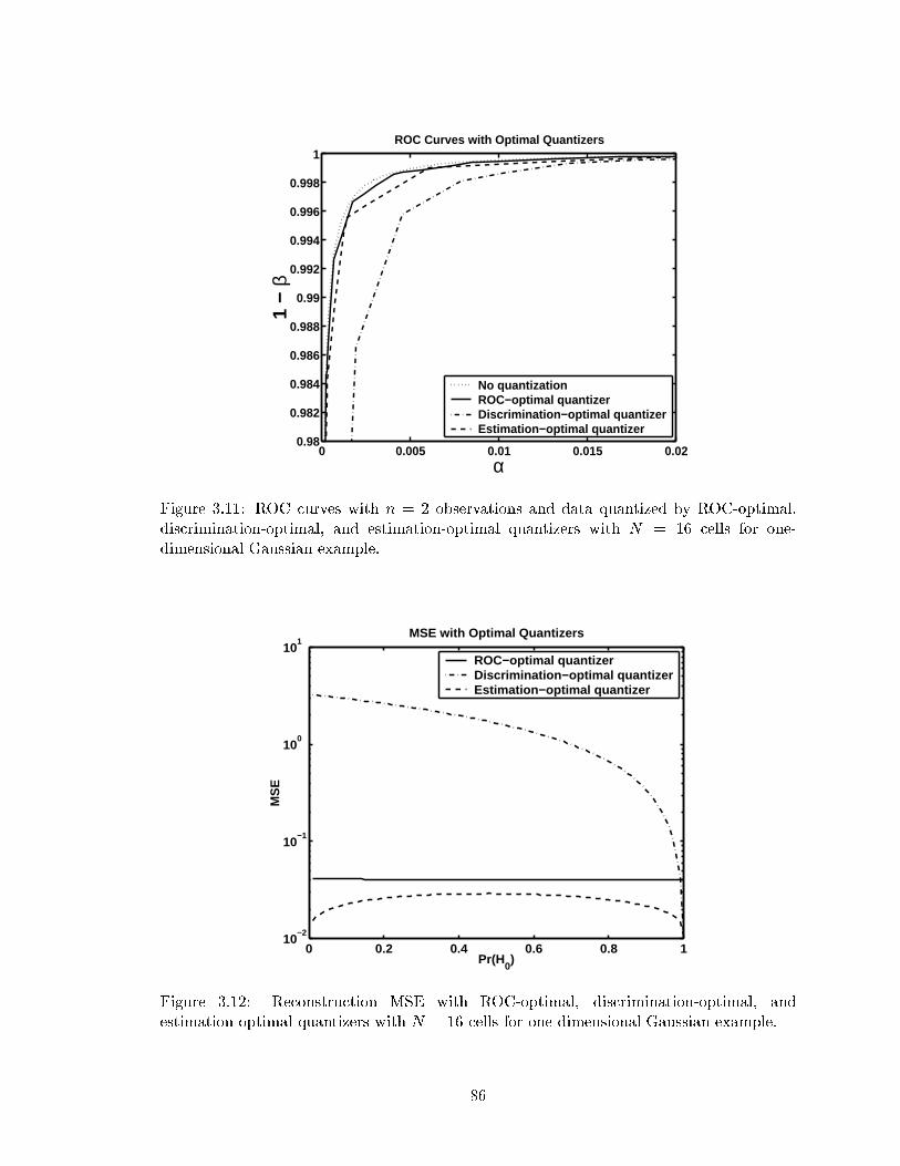
0 0.005 0.01 0.015 0.020.98
0.982
0.984
0.986
0.988
0.99
0.992
0.994
0.996
0.998
1
α
1 −
β
ROC Curves with Optimal Quantizers
No quantization ROC−optimal quantizer Discrimination−optimal quantizerEstimation−optimal quantizer
Figure 3.11: ROC curves with n = 2 observations and data quantized by ROC-optimal,discrimination-optimal, and estimation-optimal quantizers with N = 16 cells for one-dimensional Gaussian example.
0 0.2 0.4 0.6 0.8 110
−2
10−1
100
101
Pr(H0)
MS
E
MSE with Optimal Quantizers
ROC−optimal quantizer Discrimination−optimal quantizerEstimation−optimal quantizer
Figure 3.12: Reconstruction MSE with ROC-optimal, discrimination-optimal, andestimation-optimal quantizers with N = 16 cells for one-dimensional Gaussian example.
86

Cherno�-Information-Optimal Quantizer
Equal-variance Gaussian sources permit an additional optimization procedure: maxi-
mization of Cherno� information. Recall that the Cherno� information C, given in equa-
tion (3.16), is the greatest possible exponent in the probability of error of a Bayes test.
Note from equation (3.16) that maximization of Cherno� information is equivalent to max-
imizing L(q��k�q0) = L(q��k�q1) where �� is chosen such that the two discriminations are
equal. Thus, this optimization criterion di�ers from the ROC optimality criterion in that
the parameter � is �xed.
Again, assume the sources given by (3.54). It can easily be shown that the tilted density
is Gaussian with unit variance:
q� � N (��; 1)
where �� = (1� �)�0 + ��1. The log-likelihood ratios �0(x) and �1(x) given by (3.35) are
�0(x) = �1
2(�� � �0)
2 + x(�� � �0)
�1(x) = �1
2(�� � �1)
2 + x(�� � �1):
Now, the discrimination loss �L0;N given in equation (3.33) can be written
�L0;N � F2N2=k
Zq�(x)
�(x)2=kdx��2 + �(1� �) (Eq� [�0(x)]�Ep[�0(x)])
�
where
Eq�[�0(x)] =
Zq�(x)�0(x)dx; Ep[�0(x)] =
Zp(x)�0(x)dx;
and
p(x) =q�(x)=�(x)
2=kRq�(y)=�(y)2=kdy
:
Note that the Fisher covariation pro�le F is constant. If the point density �(x) is symmetric
about ��, then the \density" p(x) is also symmetric about ��. Since �0(x) is linear in x, it
87

is easily seen that Eq�[�0(x)] = Ep[�0(x)] and thus
�L0;N � �2F2N2=k
Zq�(x)
�(x)2=kdx:
By similar arguments it can be shown that
�L1;N � (1� �)2F2N2=k
Zq�(x)
�(x)2=kdx:
To maximize Cherno� information, the discriminations L0 and L1 must be equal. It is
easy to see that using � = 1=2 gives this result. The Cherno�-information-optimal point
density for the Gaussian sources given by (3.54) is thus
�Ch(x) =q1=2(x)
1=3Rq1=2(y)1=3dy
:
For �0 = 0 and �1 = 8, Figure 3.13 shows the optimal point density for Cherno�
information �Ch, along with the ROC-optimal point density �o. Both point densities are
maximized at x = 4, where the two source densities cross. The Cherno�-information-
optimal quantizer places more emphasis at this point, however. In Figure 3.14, the L1(L0)
curve is plotted along with the quantized curves for both quantizers with N = 8 cells. Note
that the intersection of each of these curves with the unit-slope line gives the corresponding
Cherno� information. The Cherno�-optimal curve lies above the ROC-optimal curve in
a region close to the intersection with the unit-slope line, thus yielding greater Cherno�
information. On the other hand, the area under the ROC-optimal curve is greater, as
expected. Note that the Cherno�-optimal quantizer is optimized speci�cally for � = 1=2,
and not for any other value of �.
Finally, we note that this analysis can be extended to obtain higher-dimensional Cherno�-
information-optimal VQ's for Gaussian sources with identity covariance matrices. For these
cases, we must restrict attention to quantizers with point densities and covariation pro�les
that are symmetric about ��, the mean of the tilted density. For example, restricted polar
quantizers [45] and some shape-gain quantizers [27] satisfy this constraint.
88
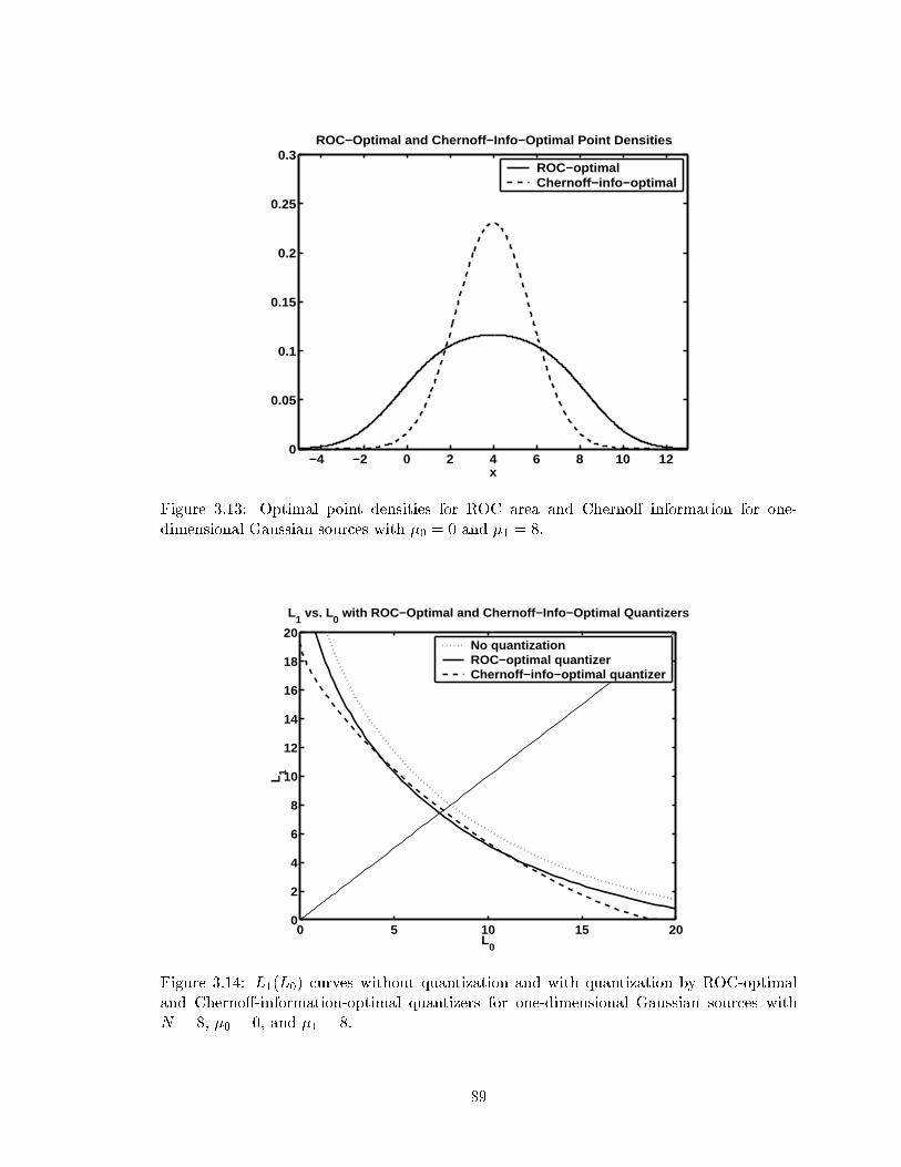
−4 −2 0 2 4 6 8 10 120
0.05
0.1
0.15
0.2
0.25
0.3
x
ROC−Optimal and Chernoff−Info−Optimal Point Densities
ROC−optimal Chernoff−info−optimal
Figure 3.13: Optimal point densities for ROC area and Cherno� information for one-dimensional Gaussian sources with �0 = 0 and �1 = 8.
0 5 10 15 200
2
4
6
8
10
12
14
16
18
20
L0
L 1
L1 vs. L
0 with ROC−Optimal and Chernoff−Info−Optimal Quantizers
No quantization ROC−optimal quantizer Chernoff−info−optimal quantizer
Figure 3.14: L1(L0) curves without quantization and with quantization by ROC-optimaland Cherno�-information-optimal quantizers for one-dimensional Gaussian sources withN = 8, �0 = 0, and �1 = 8.
89
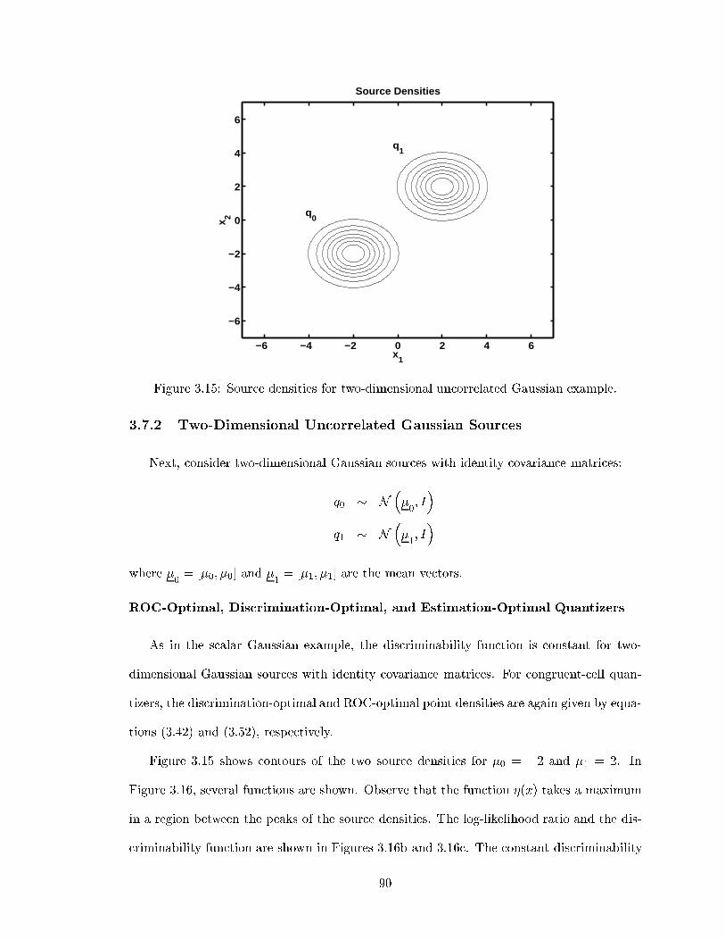
−6 −4 −2 0 2 4 6
−6
−4
−2
0
2
4
6
x1
x 2
Source Densities
q0
q1
Figure 3.15: Source densities for two-dimensional uncorrelated Gaussian example.
3.7.2 Two-Dimensional Uncorrelated Gaussian Sources
Next, consider two-dimensional Gaussian sources with identity covariance matrices:
q0 � N��0; I�
q1 � N��1; I�
where �0= [�0; �0] and �1 = [�1; �1] are the mean vectors.
ROC-Optimal, Discrimination-Optimal, and Estimation-Optimal Quantizers
As in the scalar Gaussian example, the discriminability function is constant for two-
dimensional Gaussian sources with identity covariance matrices. For congruent-cell quan-
tizers, the discrimination-optimal and ROC-optimal point densities are again given by equa-
tions (3.42) and (3.52), respectively.
Figure 3.15 shows contours of the two source densities for �0 = �2 and �1 = 2. In
Figure 3.16, several functions are shown. Observe that the function �(x) takes a maximum
in a region between the peaks of the source densities. The log-likelihood ratio and the dis-
criminability function are shown in Figures 3.16b and 3.16c. The constant discriminability
90

−5 0 5
−6
−4
−2
0
2
4
6
η(x)
(a)−5 0 5
−6
−4
−2
0
2
4
6
Log−Likelihood Ratio
(b)
−10
0
10
−10
0
1031
31.5
32
32.5
33
Discriminability || ∇ Λ(x) ||2
−5 0 5
−6
−4
−2
0
2
4
6
ROC−Optimal Point Density
(d)
−5 0 5
−6
−4
−2
0
2
4
6
Discrimination−Optimal Point Density
(e)−5 0 5
−6
−4
−2
0
2
4
6
Estimation−Optimal Point Density
(f)
(c)
Figure 3.16: Two-dimensional uncorrelated Gaussian example: (a) �(x), (b) log-likelihood ratio �(x), (c) discriminability kr�(x)k2, (d) ROC-optimal point density, (e)discrimination-optimal point density, (f) estimation-optimal point density.
91

−5 0 5−5
−4
−3
−2
−1
0
1
2
3
4
5
x1
x 2
ROC−Optimal VQ
Figure 3.17: ROC-optimal 64-cell vector quantizer for two-dimensional uncorrelated Gaus-sian example.
function results in the ROC-optimal point density having contours aligned with those of
�(x) and the discrimination-optimal point density having contours aligned with those of q0.
Finally, the estimation-optimal point density for equal priors is shown in Figure 3.16f.
The two-dimensional congruent-cell quantizers with N = 64 cells with the ROC-optimal,
discrimination-optimal, and estimation-optimal point densities are shown in Figures 3.17,
3.18, and 3.19, respectively. These quantizers were again obtained using the generalized
Lloyd, or LBG algorithm. This algorithm and its utility for obtaining optimal congruent-
cell quantizers is described in Appendix F.
The hypothesis testing performance of the 64-cell quantizers in Figures 3.17, 3.18, and
3.19 is compared in Figure 3.20. Similar to the scalar Gaussian example, the ROC-optimal
quantizer performs the best, while the discrimination-optimal quantizer yields the largest
discrimination between quantized sources, but performs poorly on average.
92

−5 0 5−5
−4
−3
−2
−1
0
1
2
3
4
5
x1
x 2
Discrimination−Optimal VQ
Figure 3.18: Discrimination-optimal 64-cell vector quantizer for two-dimensional uncorre-lated Gaussian example.
−5 0 5−5
−4
−3
−2
−1
0
1
2
3
4
5
x1
x 2
Estimation−Optimal VQ
Figure 3.19: Estimation-optimal 64-cell vector quantizer for two-dimensional uncorrelatedGaussian example.
93

0 2 4 6 8 100
2
4
6
8
10
12
14
16
L0
L 1
L1 vs. L
0 Curves with Optimal Quantizers
No quantization ROC−optimal quantizer Discrimination−optimal quantizerEstimation−optimal quantizer
Figure 3.20: L1(L0) curves without quantization and with quantization by ROC-optimal,discrimination-optimal, and estimation-optimal quantizers with N = 64 cells for two-dimensional uncorrelated Gaussian example. ROC-optimal quantizer has best performance,on average, while detection-optimal quantizer yields largest value of L(�q0k�q1).
Optimal Log-Likelihood Ratio Quantizer
Next, the optimal log-likelihood ratio quantizer for this example is obtained by �rst
noting that the log-likelihood ratio �(x) is
�(x) =1
2
�k�
1k2 � k�
0k2�+ (�0 � �1)(x1 + x2)
where x1 and x2 are the two components of the source vector x. Thus, the densities q�;0(l)
and q�;1(l) of the log-likelihood ratio under the two hypotheses are Gaussian and the ROC-
optimal constituent quantizer Q�, which quantizes �(x), is easily obtained. The cells and
codebook points of the resultant ROC-optimal LLR quantizer with N = 64 are shown in
Figure 3.21. Note that the codebook points are arbitrarily chosen to lie in the centroids of
their cells. Each cell boundary is a level set (contour) of �(x) (see Figure 3.16b).
The hypothesis testing performance of the 64-cell ROC-optimal LLR quantizer is com-
pared to that of the 64-cell ROC-optimal congruent-cell quantizer in Figure 3.22. Observe
that the LLR quantizer yields better hypothesis testing performance. The reconstruction
94

−5 0 5−5
−4
−3
−2
−1
0
1
2
3
4
5
x1
x 2
LLR VQ
Figure 3.21: Optimal 64-cell log-likelihood ratio quantizer for two-dimensional uncorrelatedGaussian example.
0 2 4 6 8 10 12 14 160
2
4
6
8
10
12
14
16
L0
L 1
L1 vs. L
0 Curves with Optimal Quantizers
ROC−optimal small−cell quantizerROC−optimal LLR quantizer
Figure 3.22: L1(L0) curves with 64-cell ROC-optimal congruent-cell quantizer and 64-cellROC-optimal LLR quantizer for two-dimensional uncorrelated Gaussian example.
95
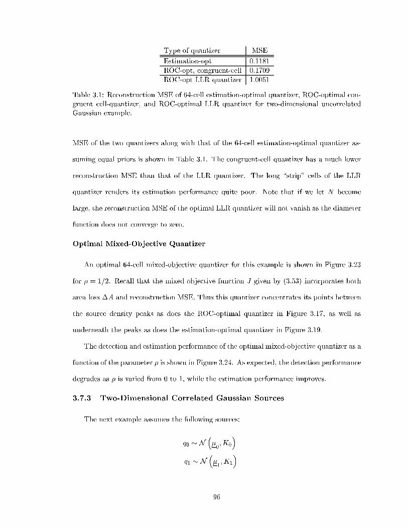
Type of quantizer MSE
Estimation-opt 0.1181
ROC-opt, congruent-cell 0.1709
ROC-opt LLR quantizer 1.0051
Table 3.1: Reconstruction MSE of 64-cell estimation-optimal quantizer, ROC-optimal con-gruent cell-quantizer, and ROC-optimal LLR quantizer for two-dimensional uncorrelatedGaussian example.
MSE of the two quantizers along with that of the 64-cell estimation-optimal quantizer as-
suming equal priors is shown in Table 3.1. The congruent-cell quantizer has a much lower
reconstruction MSE than that of the LLR quantizer. The long \strip" cells of the LLR
quantizer renders its estimation performance quite poor. Note that if we let N become
large, the reconstruction MSE of the optimal LLR quantizer will not vanish as the diameter
function does not converge to zero.
Optimal Mixed-Objective Quantizer
An optimal 64-cell mixed-objective quantizer for this example is shown in Figure 3.23
for � = 1=2. Recall that the mixed objective function J given by (3.53) incorporates both
area loss �A and reconstruction MSE. Thus this quantizer concentrates its points between
the source density peaks as does the ROC-optimal quantizer in Figure 3.17, as well as
underneath the peaks as does the estimation-optimal quantizer in Figure 3.19.
The detection and estimation performance of the optimal mixed-objective quantizer as a
function of the parameter � is shown in Figure 3.24. As expected, the detection performance
degrades as � is varied from 0 to 1, while the estimation performance improves.
3.7.3 Two-Dimensional Correlated Gaussian Sources
The next example assumes the following sources:
q0 � N��0;K0
�q1 � N
��1;K1
�
96
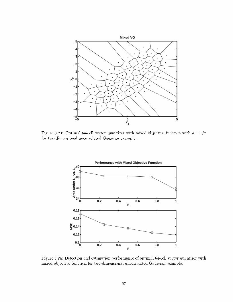
−5 0 5−5
−4
−3
−2
−1
0
1
2
3
4
5
x1
x 2
Mixed VQ
Figure 3.23: Optimal 64-cell vector quantizer with mixed objective function with � = 1=2for two-dimensional uncorrelated Gaussian example.
0 0.2 0.4 0.6 0.8 134
36
38
40
Are
a un
der
L1 v
s. L
0
Performance with Mixed Objective Function
ρ
0 0.2 0.4 0.6 0.8 10.1
0.12
0.14
0.16
0.18
ρ
MS
E
Figure 3.24: Detection and estimation performance of optimal 64-cell vector quantizer withmixed objective function for two-dimensional uncorrelated Gaussian example.
97

−6 −4 −2 0 2 4 6
−6
−4
−2
0
2
4
6
x1
x 2
Source Densities
q0
q1
Figure 3.25: Source densities for two-dimensional correlated Gaussian example.
where �0= [�2;�2], �
1= [2; 2], and
K0 =
264 3 �2:5
�2:5 3
375 ; K1 =
264 3 2:5
2:5 3
375 :
The source densities are shown in Figure 3.25.
Figure 3.26 shows several functions associated with this example. Unlike the uncorre-
lated Gaussian example, the discriminability function is not constant. Recall that equations
(3.42) and (3.52) give the discrimination-optimal and ROC-optimal point densities assum-
ing congruent cells. The contours of the discrimination-optimal and ROC-optimal point
densities are therefore no longer aligned with those of q0(x) and �(x) as was the case when
the discriminability function was constant.
The 64-point optimal congruent-cell quantizers are shown in Figures 3.27, 3.28, and 3.29.
The hypothesis testing performance of these quantizers is compared in Figure 3.30, which
shows their L1(L0) curves. As in the two previous examples, the ROC-optimal quantizer
has the best performance (maximum area) of all three quantizers and the discrimination-
optimal quantizer yields the largest value of L(�q0k�q1).
98

−5 0 5
−6
−4
−2
0
2
4
6
η(x)
(a)
maximum
−5 0 5
−6
−4
−2
0
2
4
6
Log−Likelihood Ratio
(b)
−5 0 5
−6
−4
−2
0
2
4
6
(c)
Discriminability || ∇ Λ(x) ||2
minimum
−5 0 5
−6
−4
−2
0
2
4
6
ROC−Optimal Point Density
(d)
maximum
−5 0 5
−6
−4
−2
0
2
4
6
Discrimination−Optimal Point Density
(e)
maxima
−5 0 5
−6
−4
−2
0
2
4
6
Estimation−Optimal Point Density
(f)
maxima
Figure 3.26: Two-dimensional correlated Gaussian example: (a) �(x), (b) log-likelihood ra-tio �(x), (c) discriminability kr�(x)k2, (d) ROC-optimal point density, (e) discrimination-optimal point density, (f) estimation-optimal point density.
99

−6 −4 −2 0 2 4 6
−6
−4
−2
0
2
4
6
x1
x 2
ROC−Optimal VQ
Figure 3.27: ROC-optimal 64-cell vector quantizer for two-dimensional correlated Gaussianexample.
−6 −4 −2 0 2 4 6
−6
−4
−2
0
2
4
6
x1
x 2
Discrimination−Optimal VQ
Figure 3.28: Discrimination-optimal 64-cell vector quantizer for two-dimensional correlatedGaussian example.
100

−6 −4 −2 0 2 4 6
−6
−4
−2
0
2
4
6
x1
x 2
Estimation−Optimal VQ
Figure 3.29: Estimation-optimal 64-cell vector quantizer for two-dimensional correlatedGaussian example.
0 1 2 3 4 5 6 7 80
1
2
3
4
5
6
7
L0
L 1
L1 vs. L
0 Curves with Optimal Quantizers
No quantization ROC−optimal quantizer Discrimination−optimal quantizerEstimation−optimal quantizer
Figure 3.30: L1(L0) curves without quantization and with quantization by ROC-optimal,discrimination-optimal, and estimation-optimal quantizers with N = 64 cells for two-dimensional correlated Gaussian example. ROC-optimal quantizer has best performance,on average, while detection-optimal quantizer yields largest value of L(�q0k�q1).
101

3.7.4 Triangular Sources
We now consider hypothesis testing with scalar, �nite-support, linear densities. Let the
densities be given by
q0(x) = 2x+ 1; jxj � 1=2
q1(x) = �2x+ 1; jxj � 1=2
with q0(x) = q1(x) = 0 for jxj > 1=2.
Figure 3.31 shows the source densities as well as �(x), the log-likelihood ratio gradient,
and the ROC-optimal point density. Similar to the one-dimensional Gaussian example,
we see that �(x) takes a maximum at the point x = 0 where the two densities cross.
The gradient of the log-likelihood ratio increases in magnitude as jxj increases. Thus, the
discriminability is largest near the endpoints of the interval B = [�1=2; 1=2]. The ROC-
optimal point density also increases as jxj increases. This implies that more points should
be placed near the endpoints of B, rather than near the center. Recall from equation (3.52)
that for k = 1 the ROC-optimal point density is
�o(x) =[kr�(x)k2�(x)]1=3R[kr�(y)k2�(y)]1=3dy : (3.55)
Thus, the shape of the optimal point density is determined by the product of the discrim-
inability function and �(x). For this example, the discriminability function is convex [ while
�(x) is convex \. The point density is convex [ since the curvature of the discriminability
function is greater than that of �(x).
It may seem counterintuitive that the ROC-optimal quantizer should cluster more points
near the endpoints of B as opposed to the center where the densities cross, as in the Gaus-
sian case (Section 3.7.1). Recall, however, that in the Gaussian case, the discriminability
function is constant and thus does not a�ect the optimal point density. In this example,
the discriminability has a signi�cant impact on the optimal point density. The importance
of the discriminability can be seen by comparing the L1(L0) curves for various quantizers.
102

−0.5 0 0.50
0.5
1
1.5
2
Source Densities
(a)
q0
q1
−0.5 0 0.50
0.05
0.1
0.15
0.2
0.25
0.3
0.35
0.4
η(x)
(b)
−0.5 0 0.50
10
20
30
40
50∇ Λ(x)
(c)−0.5 0 0.50
1
2
3
4
5Point Density ζ(x)
(d)
Figure 3.31: Triangular source example: (a) source densities, (b) �(x), (c) gradient (deriva-tive) of log-likelihood ratio, (d) ROC-optimal point density.
103

N AL AoL A�
L
4 0.1543 0.1120 0.1066
8 0.1543 0.1408 0.1344
16 0.1543 0.1503 0.1469
32 0.1543 0.1527 0.1508
Table 3.2: Areas under L1(L0) curves without quantization and with quantization for one-dimensional triangular example. AL = area with no quantization, Ao
L = area after quan-tization with ROC-optimal quantizer, A�
L = area after quantization with quantizer usingpoint density ��.
De�ne the suboptimal point density �� as
��(x) =�(x)1=3R�(y)1=3dy
:
This can be viewed as the optimal point density when the discriminability function is
neglected. Figure 3.32 shows the L1(L0) curve along with the corresponding curves after
quantization with eight-cell scalar quantizers using point densities �o and ��. The quantizers
were obtained using the Lloyd algorithm (see Appendix F). The quantizer with point density
�o outperforms that with point density �� as its curve is uniformly greater. Similar results
were obtained using quantizers with 3 � N � 32. Let the areas under the L1(L0) curves with
no quantization, quantization with point density �o, and quantization with point density ��,
be de�ned as AL, AoL, and A
�L, respectively. Table 3.2 shows these areas for N = 4; 8; 16;
and 32. For all cases, the ROC-optimal quantizer outperforms the quantizer with point
density ��.
Further evidence of the optimality of �o for this example can be seen by comparing the
areas under the ROC curves obtained with each of the quantizers (using �o and ��) for
reasonably large values of n. From equation (3.31) and Figure 3.32, the ROC curve area
should be larger for a quantizer using point density �o than for a quantizer using �� for
large n. Let AoROC be the area under the ROC curve when the data is quantized with point
density �o. Similarly, let A�ROC be the area when point density �� is used. Note that we are
assuming a randomized Neyman-Pearson test [35] to get a continuous ROC curve. Next,
104

�AROC n = 3 n = 4 n = 5
N = 4 �6:79 � 10�4 1:53� 10�5 2:46 � 10�4
N = 5 �1:61 � 10�4 3:62� 10�4 4:65 � 10�4
N = 6 3:88 � 10�4 6:45� 10�4 6:07 � 10�4
N = 7 5:60 � 10�4 6:76� 10�4 5:87 � 10�4
N = 8 4:68 � 10�4 5:71� 10�4 4:97 � 10�4
Table 3.3: Di�erence in ROC curve areas for one-dimensional triangular example. �AROC =AoROC�A�
ROC where AoROC = area under ROC curve after quantization with ROC-optimal
quantizer and A�ROC = area under ROC curve after quantization with quantizer using point
density ��.
de�ne �AROC = AoROC�A�
ROC. Table 3.3 shows the di�erence in areas �AROC for various
values of N and n. As n becomes large, the di�erence in area is positive. Thus, although
seemingly counterintuitive, clustering points near the endpoints of the interval B is optimal
for detection when the number of observations is reasonably large.
It is important to note that for n = 1 observation, the asymptotic formulas (3.15) do
not apply and the optimal point density �o will not necessarily produce an ROC curve with
maximum area. In fact, if the likelihood ratio is monotonic in x, as it is in this example, the
quantized ROC curve will intersect the unquantized ROC curve in up to N +1 points. The
borders of the one-dimensional quantizer cells correspond to the Neyman-Pearson thresholds
at which the intersections occur. Thus, for n = 1, the optimal quantizer should concentrate
points in areas corresponding to regions of large curvature [66] on the ROC curve. For this
example, this region is near the origin. Thus, the optimal quantizer for n = 1 di�ers greatly
from the optimal quantizer for n� 1.
In Figure 3.33, the log-likelihood ratio �(x) is plotted. Note that as jxj ! 1=2, �(x)
becomes more and more steep. Thus, a quantizer that concentrates its points near x = �1=2
will preserve more values of the suÆcient statistic �(x).
105

0.1 0.15 0.2 0.25 0.3 0.35 0.4 0.45
0.1
0.15
0.2
0.25
0.3
0.35
0.4
0.45
L0
L1
L1 vs. L
0 with Point Densities ζo and ζη
No quantization ROC−optimal point density ζo
Point density ζη
Figure 3.32: L1(L0) curves for one-dimensional triangular example without quantizationand with quantization using point densities �o and ��, with N = 8 cells.
−0.5 0 0.5−6
−4
−2
0
2
4
6
x
Λ(x
)
Log−Likelihood Ratio Λ(x)
Figure 3.33: Log-likelihood ratio for one-dimensional triangular example.
106

3.7.5 Piecewise-Constant Sources
Although Section 3.3.3 showed that suÆcient quantizers always exist when the sources
are piecewise-constant, derivation of the ROC-optimal point density for piecewise-constant
sources illustrates some important concepts. As a simple example, let q0(x) be uniform on
the interval [�1; 1] and let q1(x) be
q1(x) =
8>>>>><>>>>>:
1; jxj � 1=3
1=4; 1=3 < jxj � 1
0; jxj > 1
:
It is clear that since q0 and q1 are constant on the intervals [�1;�1=3); [�1=3; 1=3], and
(1=3; 1], the likelihood ratio will also be constant on these intervals. It follows that the
tilted density along with the functions f0, f1, and � are also piecewise-constant on the
intervals. It can also be shown that �(x) > 0 for jxj < 1. Next, the derivative of the
log-likelihood ratio is given by
r�(x) = �(log 4)Æ(x + 1=3) + (log 4)Æ(x � 1=3)
where Æ(�) is the Dirac delta function. Thus, it immediately follows that the optimal point
density is zero everywhere, but at the points �1=3 and 1=3. Figure 3.34 shows the source
densities, �(x), r�(x), and the ROC-optimal point density.
A suÆcient statistic for this example is
S(x) = I[�1=3;1=3](x):
Thus it is suÆcient to know which of the intervals [�1;�1=3); [�1=3; 1=3], or (1=3; 1] con-
tains x. Therefore, any scalar quantizer that contains cells with borders (thresholds) at
�1=3 and 1=3 is a suÆcient quantizer. The asymptotic theory asserts that a many-point
quantizer must concentrate its points close to �1=3 and 1=3. This guarantees the existence
of thresholds at �1=3 and 1=3 and thus, suÆciency.
107

−1 0 10
0.2
0.4
0.6
0.8
1
Source Densities
(a)
q0
q1
−1 0 10
0.01
0.02
0.03
0.04
0.05
η(x)
(b)
−1 0 1−50
0
50∇ Λ(x)
(c)−1 0 10
5
10
15
20
25
30Point Density ζ(x)
(d)
Figure 3.34: Piecewise-constant source example: (a) source densities, (b) �(x), (c) gradient(derivative) of log-likelihood ratio, (d) ROC-optimal point density.
108
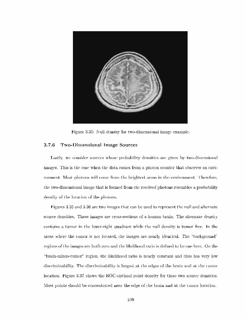
Figure 3.35: Null density for two-dimensional image example.
3.7.6 Two-Dimensional Image Sources
Lastly, we consider sources whose probability densities are given by two-dimensional
images. This is the case when the data comes from a photon counter that observes an envi-
ronment. Most photons will come from the brightest areas in the environment. Therefore,
the two-dimensional image that is formed from the received photons resembles a probability
density of the location of the photons.
Figures 3.35 and 3.36 are two images that can be used to represent the null and alternate
source densities. These images are cross-sections of a human brain. The alternate density
contains a tumor in the lower-right quadrant while the null density is tumor free. In the
areas where the tumor is not located, the images are nearly identical. The \background"
regions of the images are both zero and the likelihood ratio is de�ned to be one here. On the
\brain-minus-tumor" region, the likelihood ratio is nearly constant and thus has very low
discriminability. The discriminability is largest at the edges of the brain and at the tumor
location. Figure 3.37 shows the ROC-optimal point density for these two source densities.
Most points should be concentrated near the edge of the brain and at the tumor location.
109
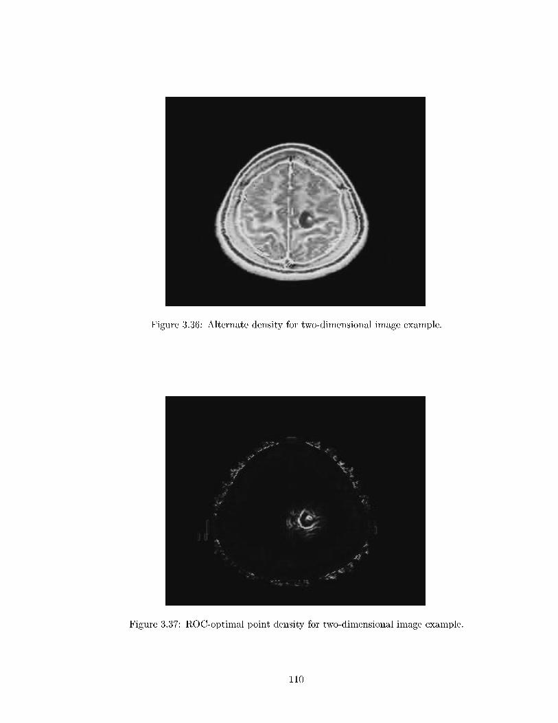
Figure 3.36: Alternate density for two-dimensional image example.
Figure 3.37: ROC-optimal point density for two-dimensional image example.
110

3.8 Conclusion
Optimal quantization procedures for distributed hypothesis testing environments have
been developed in this chapter. Conditions on the source densities under which quantizers
exist that result in no loss in hypothesis testing performance have been presented. These
conditions, given in Theorems 3.3 and 3.5, are rather restrictive and are not commonplace
in practice. Given these conditions and the asymptotic hypothesis testing performance
theory of Section 3.2.1 { including Stein's lemma and the exponential decay rates of the
probabilities of type I and II errors { the need for discrimination-based objective functions is
evident. Formulas for discrimination losses due to quantization by a many-point, small-cell
vector quantizer have been determined and shown to resemble Bennet's integral formula
for the reconstruction MSE. These formulas suggest that �ne quantization in regions where
the discriminability function is large is optimal for detection. Optimal small-cell quantizers
for maximization of the discrimination between two sources and for maximization of ROC
curve area have been derived under a congruent-cell assumption. Additionally, the optimal
ellipsoidal-cell quantizers for these two objectives have been discussed. In the limit, as
the number of quantizer cells becomes large, these quantizers preserve the log-likelihood
ratio. This conclusion points to the optimality of the log-likelihood ratio quantizer for
hypothesis testing performance. Accordingly, the optimal log-likelihood ratio quantizer
has been derived by optimizing the point density of the scalar constituent quantizer. The
estimation performance, as measured by reconstruction MSE, of the log-likelihood ratio
quantizer has been shown to be poor, due to violation of the small-cell condition, which
is required of estimation-optimal quantizers. By assuming the small cell condition, mixed
objective functions have been optimized, which can be used to trade detection performance
for estimation performance. Numerical examples of the various optimal quantizers have
been presented for several types of scalar and two-dimensional sources. These examples
have demonstrated the important concepts introduced in the chapter regarding detection
111

and estimation performance of vector quantizers. In particular, the discriminability function
and, more generally, the Fisher covariation pro�le have been shown to have signi�cant
in uence in the placement of codebook points in quantizers optimal for hypothesis testing.
112

APPENDICES
113

APPENDIX A
Derivation of Bound on Register Power Consumption
Consider a zero-mean wide-sense stationary Gaussian random sequence xk, with auto-
correlation sequence R(�) = E[xkxk+� ], uniformly quantized to B bits and loaded into a
B-bit register, whose maximum and minimum values are +1 and �1, respectively. The
quantizer cells are shown in Figure A.1.
Let nk denote the number of bits that ip when loading the value xk+1 into the register.
Then
E[nk] =BXi=1
i P (nk = i) =BXi=0
P (nk > i):
Next we note that
BXi=1
P (nk = i) �BXi=0
P (nk > i) �BXi=1
B � P (nk = i):
Therefore,
P (nk > 0) � E[nk] � B � P (nk > 0): (A.1)
Now P (nk > 0) is equal to the probability that at least one bit ips when loading xk+1 into
//// s
0�2
s
�3�2 1�
3�
2
s
1����2
s
���3�2
3�
2� 1
s
�� 1
Figure A.1: Uniform scalar quantizer.
114

k
xk+1
xk
xk+1
x
2 2∆3
2
∆
3
k
x
∆
- 12∆3
2∆31 -
x
k+1
∆
∆UT
S
Figure A.2: Regions de�ned in equation (A.3).
the register. This is equal to one minus the probability that no bits ip. Therefore
P (nk > 0) = 1� P (nk = 0): (A.2)
No bits in the register will ip if xk and xk+1 lie in the same quantizer cell. The granularity
of the quantizer is � = 2�B+1. De�ne
S =
1[m=�1
f(xk; xk+1) j xk; xk+1 2 (�(m� 1=2);�(m + 1=2))g
T = f(xk; xk+1) j xk; xk+1 2 (�1; 3�=2 � 1) [ (1� 3�=2;+1)g
U =n(xk; xk+1) j jxk � xk+1j � �=
p2o: (A.3)
These regions are shown in Figure A.2. Then P (nk = 0) = P (S [ T ) and
P (S) � P (nk = 0) � P (S) + P (T ): (A.4)
For P (S) we have,
P (S) =
1Xm=�1
Z �(m+1=2)
�(m�1=2)
Z �(m+1=2)
�(m�1=2)fxk;xk+1(x; y) dxdy
where fxk;xk+1 is the joint probability density function of xk and xk+1. For each integer m
let xm = ym = � �m. By the Mean Value Theorem, for each m there exist �xm; �ym such
115

that
P (S) =
1Xm=�1
fxk;xk+1(�xm; �ym)�2
=
1Xm=�1
fxk;xk+1(xm; ym)�2 +
1Xm=�1
�fxk;xk+1(�xm; �ym)� fxk;xk+1(xm; ym)
��2 (A.5)
Next we note that
P (U) =
1Xm=�1
"Z m�
x=(m�1)�
Z x+�
y=(2m�1)��xfxk;xk+1(x; y) dxdy +
Z (m+1)�
x=m�
Z �x+(2m+1)�
y=x��fxk;xk+1(x; y) dxdy
#:
Again by the Mean Value Theorem, there exist x0m; y0m such that
P (U) =
1Xm=�1
fxk;xk+1(x0m; y
0m)(�
p2)2
=
1Xm=�1
fxk;xk+1(xm; ym)2�2 +
1Xm=�1
�fxk;xk+1(x
0m; y
0m)� fxk;xk+1(xm; ym)
�2�2: (A.6)
From (A.5) and (A.6),
P (S) =P (U)
2+ Æ (A.7)
where Æ = �2P1
m=�1
�fxk;xk+1(�xm; �ym)� fxk;xk+1(x
0m; y
0m)�. Now P (T ) can be bounded
using the Chebyshev inequality:
P (T ) = P (jxkj � 1� 3�=2; jxk+1j � 1� 3�=2)
� R(0) (A.8)
where = (1� 3�=2)�2.
From (A.2), (A.4), (A.7), and (A.8)
1� P (U)
2� (Æ + R(0)) � P (nk > 0) � 1� P (U)
2� Æ:
116
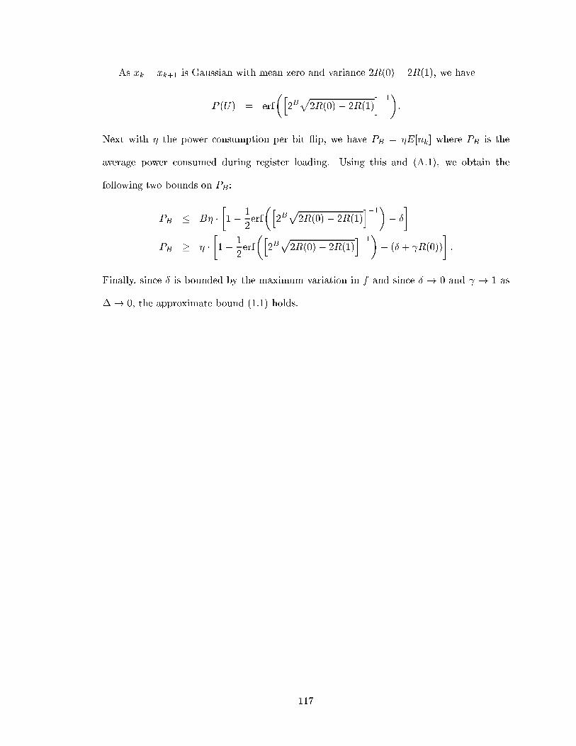
As xk � xk+1 is Gaussian with mean zero and variance 2R(0)� 2R(1), we have
P (U) = erf
�h2Bp2R(0) � 2R(1)
i�1�:
Next with � the power consumption per bit ip, we have PB = �E[nk] where PB is the
average power consumed during register loading. Using this and (A.1), we obtain the
following two bounds on PB :
PB � B� ��1� 1
2erf
�h2Bp2R(0) � 2R(1)
i�1�� Æ
�
PB � � ��1� 1
2erf
�h2Bp2R(0)� 2R(1)
i�1�� (Æ + R(0))
�:
Finally, since Æ is bounded by the maximum variation in f and since Æ ! 0 and ! 1 as
�! 0, the approximate bound (1.1) holds.
117
APPENDIX B
Iteration Power of LMS Algorithm
We consider a hardware implementation of the �nite-precision LMS algorithm in which
all data are stored in Bd + 1 bits and all coeÆcients in Bc + 1 bits. We assume that all
right-shifted quantities are rounded correctly and that right shifting consumes negligible
energy compared to additions and multiplications.
Two multipliers are used: one with Bc-bit multiplier and Bd-bit multiplicand, and one
with Bd-bit multiplier and multiplicand. Only magnitudes are multiplied and determina-
tion of input magnitude and output sign is assumed to consume negligible energy. Each
multiplier is assumed to be a direct table lookup multiplier, implemented by use of a ROM
indexed by the magnitudes of the multiplier and multiplicand, that stores the product
(magnitude) quantized to B1 + B2 bits where B1 and B2 are the number of bits used for
the multiplier and multiplicand [11]. Although the power consumed by such a multiplier is
proportional to 2B1+B2 , we use a simpli�ed formula and assume the power consumed during
a (real) multiplication is PB1�B2;real = �t(B1 +B2) where �t is the power per bit of a table
lookup operation.
A complex multiplication of a + bj stored in B1 bits plus sign by c + dj stored in
B2 bits plus sign requires four real B1-bit by B2-bit multiplications and two additions of
B1 + B2 + 1 bits. Therefore, the power consumed by such a complex multiplication is
PB1�B2;complex = 4�t(B1 + B2) + 2�a(B1 + B2 + 1) where �a is the power per bit of a real
adder.
118

In the LMS update formula given by (2.2) and (2.3), the calculation of the inner product
w0Hk x0k requires p complex multiplications of numbers stored in Bc bits plus sign by numbers
stored in Bd bits plus sign and p� 1 complex (Bd+1)-bit additions. Subtracting this inner
product from y0k requires an additional complex addition of Bd + 1 bits. Next, multiplying
the conjugate of this quantity (e0k) by x0k we have p complex multiplications in which both
multiplier and multiplicand are stored in Bd bits plus sign. Since multiplication by �
requires only a shift, we are left with the addition by w0k. This operation requires p complex
additions of Bc + 1 bits. Therefore, the total power consumed during one iteration of the
complex �nite-precision LMS algorithm is
PT = 4p�t(3Bd +Bc) + 2p�a(3Bd +Bc + 2) + 2p�a(Bd +Bc + 2)
which is equivalent to (2.4).
We can derive a similar formula for multiplication using partial product accumulation.
In such a multiplier, each real B1-bit by B2-bit multiplication requires approximately B1
additions of B2 bits [38] and therefore has a power consumption of B1B2�a. The total
real operations are the same as with the table lookup multiplier. This gives the following
relation for LMS iteration power using partial product accumulation multiplication:
PT = 4p�a(B2d +BdBc + 2Bd +Bc + 2): (B.1)
Using equations (2.4) and (B.1) along with (2.19), we can plot PT as a function of BT
for both power relations. These plots are shown in Figure B.1 for � = 1=2, �a � 1:4 mW,
�t � 6:8 mW, and p = 2. Note that the formula derived using partial product accumulation
is quadratic in BT while the formula derived using table lookup multiplication is linear in
BT .
119

0 5 10 15 20 25 300
1
2
3
4
5
6
BT
PT (W
atts
)
PT vs. B
T
Table Lookup Partial Product
Figure B.1: PT versus BT for di�erent power relations with �a � 1:4 mW and �t � 6:8 mW.
120

APPENDIX C
Derivation of Mean Convergence Rate, Weight-ErrorCovariance, and Excess Mean Square Error
From (2.2) and (2.3), we see that the �nite precision LMS update is of the form
w0k+1 = w0k + �x0k(y0�k � x0Hk w0k + �k) + �k
where ��k and �k are approximated as zero-mean, white, and uncorrelated with all other
signals. The variance of �k is 2p�2d and the variance of each component of �k is 2�
2c .
C.1 Mean Convergence Rate
Using the method of [65] we obtain (2.7). First de�ne
Æw0k+1 = w0k+1 � w0k = �x0ke0�k + �k
and
�0k = y0k � w0oHx0k; ~w0k = w0k � w0o:
Then we have
e0k = �0k � ~w0Hk x0k + ��k:
Next, use ~w0k+1 � ~w0k = Æw0k+1 to obtain
~w0k+1 = (I � �x0kx0Hk )~w0k + �x0k�
0�k + �x0k�k + �k: (C.1)
121

Similar to [65], we assume that x0k and �0k are independent. Using this and the fact that �k
and �k have zero means, we see that
E[ ~w0k+1jx01; : : : ; x0k�1; �01; : : : ; �0k�1] = ~w0k � �Rx0 ~w0k
and taking expectations,
E[ ~w0k+1] = (I � �Rx0)E[ ~w0k]
which is completely analogous to the in�nite-precision LMS algorithm. Using the same
analysis as in [65, Sec. 5.2], we conclude that E[w0k]! w0o as long as condition (2.6) is met.
C.2 Steady-State Weight-Error Covariance and ExcessMean Square Error
We begin our derivation of (2.8) and (2.10) in the manner of [15]. We �rst write the
weight update formula for the in�nite-precision LMS algorithm
wk+1 = wk + � xk�y�k � xHk wk
�: (C.2)
We de�ne
�2d =1
122�2Bd ; �2c =
1
122�2Bc : (C.3)
These are the variances of the quantization noises associated with quantizers having Bd and
Bc bits (plus sign), respectively. We use primed symbols to represent quantized values and
de�ne the following quantities
x0k = xk + �k
y0k = yk + �k
w0k = wk + �k: (C.4)
The components of the vector �k and �k are complex numbers whose real and imaginary
parts are assumed uncorrelated and have variances �2d. Therefore, the variance of �k and
of each component of �k is 2�2d.
122

Thus we have the representation for the quantized value of the �lter output
y0k = Qd(w0Hk x0k) = wH
k xk + �Hkxk + wH
k �k + �k (C.5)
where �k is de�ned above. As in [15], we have ignored the noise product term �Hk�k in
(C.5), as its power is of order �2d�2c .
The total error is now
sk � s0k =1
a(yk �wH
k xk)�1
a(�H
kxk + wH
k �k + �k): (C.6)
The �rst term on the right-hand side of (C.6) is the error of the in�nite-precision algorithm.
The second term is the error due to quantization and will be denoted eq. Under the hypoth-
esis (2.5), these terms are uncorrelated and the MSE for the �nite-precision LMS algorithm
is
� =1
a2E[jyk � wH
k xkj2] +1
a2E[j�H
kxk + wH
k �k + �kj2]: (C.7)
The �rst term on the right-hand side of (C.7) is the MSE of the in�nite-precision LMS
algorithm and is equal to �min+ �excess [65, 74]. The second term is the excess MSE due to
quantization
�q = E[jeqj2]:
Under the assumptions (2.5), �k, �k, �k, and �k are all uncorrelated and
�q =1
a2
�E[j�H
kxkj2] +E[jwH
k �kj2] +E[j�kj2]�: (C.8)
The term E[j�kj2] is equal to 2p �2d. For the term E[jwHk �kj2] we obtain
E[jwHk �kj2] = 2�2d E[kwkk2]:
Note that this di�ers from the real case studied in [15] by a factor of two. In the steady
state, this becomes
E[jwHk �kj2] = 2�2d
�kwok2 + 1
2p��min
�: (C.9)
123

Finally, for the �rst term in (C.8)
E[j�Hkxkj2] = tr(RxPk) (C.10)
where Pk = E[�k�Hk].
To derive an expression for Pk, we assume � is small and use the averaged system
techniques of [65, Sec. 9.2]. De�ne �w0k as the weight vector at time k of the averaged
�nite-precision system. Similarly, let �wk be the averaged in�nite-precision system weight
vector. Then the �nite-precision primary system obeys the recursion (C.1)
~w0k+1 = (I � �x0kx0Hk )~w0k + �x0k�
0�k + �x0k�k + �k:
while the �nite-precision averaged system recursion is
�w0k+1 = (I � �Rx0)�w0k: (C.11)
Next de�ne uk = (wk � �wk)=p� and u0k = (w0k � �w0k)=
p�. Finally, de�ne
� = limk!1
E[ukuHk ]
�0 = limk!1
E[u0ku0Hk ]:
Now write
w0k � �w0k = (w0k �wk) + (wk � �wk) + (�wk � �w0k): (C.12)
Assuming that the �rst two terms on the right-hand side of (C.12) are uncorrelated and
that the last term is small we have
P = limk!1
Pk = �(�0 � �): (C.13)
To apply the averaged system techniques of [65] to the �nite-precision algorithm, it is
necessary that the following conditions hold
lim�!0
�d = 0
lim�!0
�c = 0 (C.14)
124

where �c = 2�Bc and �d = 2�Bd . In the �xed-point, power-of-two algorithm, the magni-
tude of x0ke0�k is stored in 2Bd bits before shifting to the right by q = � log2 � bits. Therefore,
we require q � 2Bd. To avoid slowdown we require Bc > Bd+�. These requirements ensure
that (C.14) holds.
Assuming �k is white and independent of xk, we have
� =�min
2I: (C.15)
Proceeding as in [65] for the �nite-precision system, assuming �0 is white, using (C.1) and
(C.11) we �nd that �0 satis�es the following equation
Rx0�0 + �0Rx0 = (�2�0 + 2p�2d)Rx0 +
2
�2�2cI
where �2�0 = E[j�0j2]. It is easy to show that Rx0 and �0 have the same eigenvectors and
�0 =1
2(�2�0 + 2p�2d)I +
2
�2�2cR
�1x0 :
Next, using �2�0 = RHx0y0R
�1x0 Rx0y0 � �min + 2�2d and (C.13) gives
P = �(p+ 1)�2dI +1
��2cR
�1x0 : (C.16)
Finally, using Rx0 � Rx in (C.16) yields
tr(RxP ) = �(p+ 1)�2dtr(Rx) +p�2c�: (C.17)
As the �rst term on the right hand side of (C.17) is of order ��2d, it can be ignored.
Now, using (C.8), (C.9), and (C.17) we get
�q =1
a2
�p �2c�
+ 2�2d (kwok2 + p)
�
from which, by using (C.3), we obtain (2.10).
125
APPENDIX D
Derivation of Optimal Bit Allocation Factors
D.1 Total Bit Budget
Using equations (2.10) and (2.19) we can write the excess MSE due to quantization as
�q = �c2�2(1��)BT + �d2
�2�BT : (D.1)
Di�erentiating this equation with respect to � we get
d�qd�
= 2 ln 2 BT
��c2
�2(1��)BT � �d2�2�BT
�: (D.2)
Di�erentiating again we get
d2�qd�2
= (2 ln 2 BT )2 �q > 0: (D.3)
Equation (D.3) shows that for � 2 [0; 1],d2�qd�2 > 0 and therefore �q is a convex function of
�. Now, settingd�qd� in (D.2) equal to zero at � = ��, we have
�d�c
= 24��BT�2BT : (D.4)
Equation (D.4) leads directly to (2.20).
D.2 Total Power Budget
To derive (2.23) we �rst de�ne the following constants
A = PT � 8p�a; B = 8p(�a + �t); C = 2p�a: (D.5)
126

Then from (2.22) we have
BT =A
B�+ C: (D.6)
Di�erentiating (D.1) with respect to � gives
d�qd�
= ln2 �c 2�2(1��)BT � d
d�[�2(1 � �)BT ] +
ln 2 �d 2�2� BT � d
d�[�2� BT ]: (D.7)
Di�erentiating again and using (D.6), we have
d2�qd�2
= ln2 �c 2�2(1��)BT
��4AB(B +C)
(B�+ C)3+ ln2 � 4A
2(B + C)2
(B�+ C)4
�+
ln2 �d 2�2�BT
�4ABC
(B�+ C)3+ ln2 � 4A2C2
(B�+ C)4
�: (D.8)
Now, �q is convex ifd2�qd�2
is positive. From (D.8), it is clear thatd2�qd�2
will be positive if the
following condition is met:
ln 2 � 4A2(B + C)2
(B�+ C)4>
4AB(B + C)
(B�+C)3:
Using (D.5) and (D.6), this condition will be satis�ed if and only if the following condition
is satis�ed:
BT >B
ln 2(B + C)=
1
ln 2
�1� �a + �t
2�a + 3�t
�: (D.9)
The term on the right-hand side of (D.9) is clearly less than 1= ln 2. This means thatd2�qd�2
will be positive if BT > 1= ln 2. This condition is clearly true under the assumption BT � 2.
Therefore, �q is once again a convex function of �. To solve for ��� we setd�qd� equal to zero.
Using (D.7) we have
�c 2�2(1����)� A
B���+C � 2A(B + C)
(B��� + C)2= �d 2
�2���� AB���+C � 2AC
(B��� + C)2:
This implies
��� =2A+ C log2
��d�c� CB+C
�4A�B log2
��d�c� CB+C
� : (D.10)
Equations (D.5) and (D.10) lead to (2.23).
127

APPENDIX E
Derivation of Asymptotic Discrimination Losses
E.1 Asymptotic Loss in Discrimination Between TwoSources
To derive the asymptotic loss in discrimination (3.28) between q0 and q1, we follow the
\sequence approach" used in [13, 14, 46]. Consider a sequence of quantizers QN = (SN ; CN )
where the Nth quantizer contains the N cells SN = fSN;1; : : : ; SN;Ng and the N codebook
points CN = fxN;1; : : : ; xN;Ng. De�ne the cell probability sequences
�q0;N;i =
ZSN;i
q0(y)dy
�q1;N;i =
ZSN;i
q1(y)dy
for i = 1; : : : ; N . Note that for each N , the sets �q0;N = f�q0;N;1; : : : ; �q0;N;Ng and �q1;N =
f�q1;N;1; : : : ; �q1;N;Ng form the quantized source probability mass functions.
The log-likelihood ratio �(x) is de�ned as
�(x) = logq0(x)
q1(x)
and the sequence of log-likelihood ratios after quantization is
��N;i = log�q0;N;i�q1;N;i
:
The discrimination before quantization can be written in terms of the cells of the Nth
quantizer:
L , L(q0kq1) =NXi=1
ZSN;i
q0(y)�(y)dy:
128

The discrimination after quantization by the Nth quantizer can be written as
LN , L(�q0;Nk�q1;N ) =NXi=1
�q0;N;i��N;i:
Since our goal is to maximize the discrimination after quantization, we will refer to the
loss in discrimination as distortion. It is well known that discrimination can not increase
with processing (i.e. quantization). Thus, the distortion is nonnegative. The distortion
resulting from the Nth quantizer is thus
�LN , L� LN =
NXi=1
ZSN;i
q0(y)�(y)dy � �q0;N;i��N;i: (E.1)
Note that (E.1) is independent of the codebook CN . Therefore, we lose no generality by
assuming that the codebook points are the centroids of their cells. That is, for each N
xN;i =
RSN;i
ydy
VN;i; i = 1; : : : ; N (E.2)
where VN;i is the volume of the ith cell in the Nth quantizer. Note that (E.2) implies
ZSN;i
(y � xN;i)dy = 0; i = 1; : : : ; N:
E.1.1 Sequence De�nitions
We de�ne a few more sequences that will be necessary in analyzing the asymptotic
behavior of the quantizer sequence.
1. The sequence of diameter functions is dN (x).
2. The sequence of speci�c inertial pro�le functions is mN (x).
3. The sequence of speci�c covariation pro�le functions isMN (x). We will writeMN;i =
MN (x) for x 2 SN;i.
4. The sequence of speci�c point density functions is �N (x) = �N;i = 1=(NVN;i) for
x 2 SN;i.
129

E.1.2 Assumptions
We make several assumptions regarding the quantizers and the convergence of the se-
quences de�ned in the previous section.
1. For all N , each codebook point lies in the centroid of its cell. That is, equation (E.2)
holds.
2. The sequence of diameter functions dN (x) converges uniformly to zero.
3. The sequence of speci�c inertial pro�le functions mN (x) converges uniformly to a
function m(x), called the inertial pro�le, that is uniformly bounded by mB.
4. The sequence of speci�c covariation pro�le matrix functions MN (x) converges uni-
formly to a full-rank matrix function M(x), called the covariation pro�le.
5. The sequence of speci�c point density functions �N (x) converges uniformly to a func-
tion �(x), called the point density, that satis�esR�(x)dx = 1.
E.1.3 Notation
To facilitate the analysis, we de�ne some simplifying notation here. The density func-
tions evaluated at codebook point xN;i will be denoted
q0;N;i = q0(xN;i)
q1;N;i = q1(xN;i):
Similarly, the gradients and Hessians of q0 and q1 evaluated at xN;i will be denoted
r0;N;i = rq0(xN;i)
r1;N;i = rq1(xN;i)
r20;N;i = r2q0(xN;i)
r21;N;i = r2q1(xN;i)
130

and the log-likelihood ratio evaluated at xN;i is
�N;i = �(xN;i):
The following matrix functions will be useful in our analysis. The \Fisher" matrix function
is de�ned to be the outer product of the log-likelihood ratio gradient:
F (x) = r�(x)r�(x)T
and the matrix function G(x) is
G(x) =r2q0(x)
q0(x)� r2q1(x)
q1(x): (E.3)
In keeping with the convention set forth above, we de�ne
FN;i = F (xN;i)
GN;i = G(xN;i): (E.4)
E.1.4 Taylor Expansions
For all N , we can expand the function q0(x) in a Taylor series about the codebook points
of quantizer QN . Therefore, for all N we can write
q0(x) = q0;N;i +rT0;N;i(x� xN;i) +
1
2(x� xN;i)
Tr20;N;i(x� xN;i)
+o(kx� xN;ik2); 8x 2 SN;i: (E.5)
A similar expansion can be done for q1(x) and �(x) as shown below:
�(x) = �N;i +r�TN;i(x� xN;i) +
1
2(x� xN;i)Tr2�N;i(x� xN;i)
+o(kx� xN;ik2); 8x 2 SN;i: (E.6)
The \o" terms in (E.5) and (E.6) are explained as follows. From the de�nition of the
diameter function, we have kx�QN (x)k � dN (x) for all N and from Assumption 2 we have
kx�QN (x)k ! 0 uniformly. Therefore, given � > 0 there is an integer N0 such that for all
N � N0 and for all x 2 SN;io(kx� xN;ik2)kx� xN;ik2 < �:
131

E.1.5 Single-Cell Distortion
The distortion of the Nth quantizer given by (E.1) is a sum over the N quantizer cells
of the quantityRSN;i
q0(y)�(y)dy� �q0;N;i��N;i. We call this term the single-cell distortion of
cell SN;i. The bulk of the analysis required to determine the distortion involves studying
the single-cell distortion, which we do in this section.
Using (E.5) and (E.6) along with Assumption 1 we have
ZSN;i
q0(y)�(y)dy = q0;N;i�N;iVN;i +
ZSN;i
(y � xN;i)TAN;i(y � xN;i)dy
+
ZSN;i
o(ky � xN;ik2)dy (E.7)
where
AN;i =1
2
��N;ir2
0;N;i + q0;N;ir2�N;i +r0;N;ir�TN;i +r�N;irT
0;N;i
�: (E.8)
The last two terms in (E.8) arise due to the fact that the matrix in a quadratic form may
be transposed without a�ecting the result [36]. After some algebra, (E.8) can be written
AN;i =1
2
��N;ir2
0;N;i + q0;N;i(FN;i +GN;i)�
(E.9)
where FN;i and GN;i are given in (E.4).
To simplify (E.7), we �rst focus on the last term. For � > 0 there is an integer N0 such
that for all N � N0, the following two conditions hold:
o(ky � xN;ik2)ky � xN;ik2 � �
2mB; 8y 2 SN;i
and
jmN (y)�m(y)j � mB ;
) mN (y) � m(y) +mB � 2mB ; 8y 2 SN;i:
132

Therefore, for all N � N0,�����ZSN;i
o(ky � xN;ik2)dy����� �
ZSN;i
��o(ky � xN;ik2)�� dy
�ZSN;i
�
2mBky � xN;ik2dy
=�
2mB�mN (x)V
1+2=kN;i ; 8x 2 SN;i
� � � V 1+2=kN;i :
Therefore, the sequence ���RSN;i o(ky � xN;ik2)dy���
V1+2=kN;i
converges to zero and we will thus write
ZSN;i
o(ky � xN;ik2)dy = o�V1+2=kN;i
�:
Next, we rewrite the second term on the right-hand side of (E.7) as
ZSN;i
(y � xN;i)TAN;i(y � xN;i)dy = tr(AN;iMN;i)V
1+2=kN;i :
Therefore (E.7) becomes
ZSN;i
q0(y)�(y)dy = q0;N;i�N;iVN;i + tr(AN;iMN;i)V1+2=kN;i + o
�V1+2=kN;i
�: (E.10)
We now turn our attention to the term �q0;N;i��N;i found in (E.1). From (E.5) and (E.6)
we have
�q0;N;i��N;i = q0;N;i��N;iVN;i + tr(AN;iMN;i)V1+2=kN;i + o
�V1+2=kN;i
�(E.11)
where
AN;i =1
2��N;ir2
0;N;i: (E.12)
133

Combining (E.10) and (E.11) yields
ZSN;i
q0(y)�(y)dy � �q0;N;i��N;i = q0;N;i��N;i � ��N;i
�VN;i +
1
2
��N;i � ��N;i
�tr�r2
0;N;iMN;i
�V1+2=kN;i +
1
2q0;N;i tr ([FN;i +GN;i]MN;i)V
1+2=kN;i +
o�V1+2=kN;i
�: (E.13)
From the de�nitions of �N;i and ��N;i we have
�N;i � ��N;i = log
�q0;N;i � �q1;N;iq1;N;i � �q0;N;i
�:
Using the Taylor expansion
log a = (a� 1)� 1
2(a� 1)2 + o(ja� 1j2)
we have
�N;i � ��N;i = (l � 1)� 1
2(l � 1)2 + o(jl � 1j2)
where
l =q0;N;i � �q1;N;iq1;N;i � �q0;N;i :
Next, using (E.5)
l =q0;N;iq1;N;iVN;i +
12q0;N;itr(r2
1;N;iMN;i)V1+2=kN;i + o
�V1+2=kN;i
�q0;N;iq1;N;iVN;i +
12q1;N;itr(r2
0;N;iMN;i)V1+2=kN;i + o
�V1+2=kN;i
�and
l � 1 =1
2q1;N;itr(r2
1;N;iMN;i)V2=kN;i �
1
2q0;N;itr(r2
0;N;iMN;i)V2=kN;i + o
�V2=kN;i
�: (E.14)
Therefore, (l � 1)2 = o�V2=kN;i
�and using (E.14) and (E.3) we get
�N;i � ��N;i = �1
2tr(GN;iMN;i)V
2=kN;i + o
�V2=kN;i
�: (E.15)
134

Finally, (E.13) and (E.15) give
ZSN;i
q0(y)�(y)dy � �q0;N;i��N;i =1
2q0;N;itr(FN;iMN;i)V
1+2=kN;i + o
�V1+2=kN;i
�
=1
2q0;N;itr(FN;iMN;i)
VN;i
N2=k�2=kN;i
+
o�V1+2=kN;i
�: (E.16)
E.1.6 Total Distortion
Having calculated the single-cell distortion (E.16), the total distortion is obtained by
summing over all quantizer cells. Using (E.1) and (E.16), the total distortion of quantizer
QN is
�LN =1
2N2=k
NXi=1
q0;N;itr(FN;iMN;i)1
�2=kN;i
VN;i + o
�1
N2=k
�VN;i:
Multiplying by N2=k and taking the limit, we obtain (3.28).
E.2 Asymptotic Loss in Discrimination Between EachSource and the Tilted Source
In this section, we once again use a sequence approach to determine the asymptotic
loss in discrimination { this time between q� and q0 { due to quantization. Many of the
quantities de�ned in Section E.1 will be used in this section as well. The sequence de�nitions
and assumptions made in Sections E.1.1 and E.1.2, respectively, will all apply here, as well
as the notation de�ned in Section E.1.3. In addition, we will de�ne several new quantities
throughout this section.
We begin by writing the loss in discrimination between the tilted source q� and source
q0 due to quantization with an N -point vector quantizer as
�L0;N , L(q�kq0)� L(q�;Nk�q0;N )
=
NXi=1
ZSN;i
q�(x)�0(x)dx� q�;N;i�0;N;i (E.17)
135

where
�0(x) = logq�(x)
q0(x); �0;N;i = log
q�;N;i�q0;N;i
:
E.2.1 Notation
In keeping with the notational convention of Section E.1.3 we de�ne
q�;N;i = q�(xN;i)
r�;N;i = rq�(xN;i)
r2�;N;i = r2q�(xN;i)
and
�0;N;i = �0(xN;i):
Next we de�ne
� =
Zq0(x)
1��q1(x)�dx =
NXi=1
�N;i
�N;i =
ZSN;i
q0(x)1��q1(x)
�dx = �
ZSN;i
q�(x)dx
dN;i = �q1��0;N;i � �q�1;N;i � �N;i
dN =NXi�1
dN;i: (E.18)
Thus we can write
q�;N;i =�N;i + dN;i�+ dN
: (E.19)
E.2.2 Expansions of �N;i and dN;i
Expanding q�(x) in a Taylor series about xN;i we get the following representation for
�N;i:
�N;i = �q�;N;iVN;i +�
2
ZSN;i
(x� xN;i)Tr2
�;N;i(x� xN;i)dx+ o�V1+2=kN;i
�: (E.20)
136

It can be straightforwardly shown that the Hessian of the tilted density is
r2q�(x) = q�(x)
��r2q1(x)
q1(x)+ (1� �)
r2q0(x)
q0(x)� �(1� �)F (x)
�: (E.21)
Next, using the centroid assumption, we write
�q0;N;i = q0;N;iVN;i +1
2
ZSN;i
(x� xN;i)Tr2
0;N;i(x� xN;i)dx+ o�V1+2=kN;i
�
�q1;N;i = q1;N;iVN;i +1
2
ZSN;i
(x� xN;i)Tr2
1;N;i(x� xN;i)dx+ o�V1+2=kN;i
�(E.22)
and using the Taylor expansion
(x+ y)a = xa + axa�1y +1
2a(a� 1)xa�2y2 + o(y2) (E.23)
we obtain
�q1��0;N;i = q1��0;N;iV1��N;i +
1
2(1� �)q��0;N;iV
��N;i
ZSN;i
(x� xN;i)Tr2
0;N;i(x� xN;i)dx+
o�V2=k+1��N;i
�
and
�q�1;N;i = q�1;N;iV�N;i +
1
2�q��11;N;iV
��1N;i
ZSN;i
(x� xN;i)Tr2
1;N;i(x� xN;i)dx+ o�V2=k+�N;i
�:
Multiplying the two formulas above yields
�q1��0;N;i � �q�1;N;i = �q�;N;i
�
2q1;N;i
ZSN;i
(x� xN;i)Tr2
1;N;i(x� xN;i)dx
+1� �
2q0;N;i
ZSN;i
(x� xN;i)Tr2
0;N;i(x� xN;i)dx+ VN;i
!
+o�V1+2=kN;i
�: (E.24)
Finally, using (E.20), (E.21), and (E.24) we get
dN;i =�
2�(1� �)q�;N;i
ZSN;i
(x� xN;i)TFN;i(x� xN;i)dx+ o�V1+2=kN;i
�: (E.25)
We shall �nd the following formulas for �N;i and dN;i useful:
�N;i = �q�;N;iVN;i +�
2tr�r2
�;N;iMN;i
�V1+2=kN;i + o
�V1+2=kN;i
�(E.26)
dN;i =�
2�(1� �)q�;N;itr (FN;iMN;i)V
1+2=kN;i + o
�V1+2=kN;i
�: (E.27)
137
E.2.3 Asymptotic Values of �L0;N and �L1;N
From (E.7) and (E.8) we can write
ZSN;i
q�(x)�0(x)dx = q�;N;i�0;N;iVN;i +1
2�0;N;itr(r2
�;N;iMN;i)V1+2=kN;i +
1
2q�;N;itr
�(F 0
N;i +G0N;i)MN;i
�V1+2=kN;i + o
�V1+2=kN;i
�
where
F 0N;i = r�0;N;ir�T
0;N;i
G0N;i =
r2�;N;i
q�;N;i� r2
0;N;i
q0;N;i: (E.28)
Note that F 0N;i can be written in terms of FN;i:
F 0N;i = �2FN;i:
From (E.19), (E.26), and (E.27) we can write
q�;N;i = tN
�q�;N;iVN;i +
1
2tr(r2
�;N;iMN;i)V1+2=kN;i +
1
2�(1� �)q�;N;itr(FN;iMN;i)V
1+2=kN;i
�
+o�V1+2=kN;i
�(E.29)
where
tN =�
�+ dN:
Thus (E.17) becomes
�L0;N =NXi=1
q�;N;iVN;i
��0;N;i � tN �0;N;i
�+
1
2tr(r2
�;N;iMN;i)V1+2=kN;i
��0;N;i � tN �0;N;i
�+
1
2q�;N;itr
�(�2FN;i +G0
N;i)MN;i
�V1+2=kN;i �
�(1� �)
2tNq�;N;i�0;N;itr(FN;iMN;i)V
1+2=kN;i + o
�V1+2=kN;i
�: (E.30)
Next we use the Taylor expansion
log(x+ y) = log x+y
x� y2
2x2+ o(y2)
138

to write
�0;N;i = �0;N;i + 2r0;N;i � 1
2r20;N;i �
3
2+ o
�q�;N;i�q0;N;i
� q�;N;iq0;N;i
�2!
(E.31)
where
r0;N;i =q0;N;iq�;N;i�q0;N;iq�;N;i
:
To see that the last term in (E.31) is small, note that
q�;N;i�q0;N;i
� q�;N;iq0;N;i
=
��q1;N;i�q0;N;i
�� 1
�+ dN��q1;N;iq0;N;i
�� 1
�:
Using the Taylor expansions (E.22), after some algebra this becomes
q�;N;i�q0;N;i
� q�;N;iq0;N;i
=
�q1;N;iq0;N;i
+ o�V2=kN;i
��� 1
�+ dN��q1;N;iq0;N;i
�� 1
�
=
"�q1;N;iq0;N;i
��+ o
�V2=kN;i
�# 1
�+ dN��q1;N;iq0;N;i
�� 1
�
= ��q1;N;iq0;N;i
�� dN�(�+ dN )
+ o�V2=kN;i
�
where the second equality follows from (E.23). From (E.27) it is easily seen that
o
�q�;N;i�q0;N;i
� q�;N;iq0;N;i
�2!= o
�V2=kN;i
�:
Now, using (E.22) and (E.29), r0;N;i becomes
r0;N;i =
tNq0;N;i
�q�;N;i +
12tr(r2
�;N;iMN;i)V2=kN;i + 1
2�(1� �)q�;N;itr(FN;iMN;i)V2=kN;i
�+ o
�V2=kN;i
�q�;N;iq0;N;i +
12q�;N;itr(r2
0;N;iMN;i)V2=kN;i + o
�V2=kN;i
�
= tN
1 +
tr(r2�;N;iMN;i)
2q�;N;iV2=kN;i �
tr(r20;N;iMN;i)
2q0;N;iV2=kN;i +
1
2�(1� �)tr(FN;iMN;i)V
2=kN;i
!
+ o�V2=kN;i
�= tN
�1 +
1
2tr(G0
N;iMN;i)V2=kN;i +
1
2�(1� �)tr(FN;iMN;i)V
2=kN;i
�+ o
�V2=kN;i
�(E.32)
and
r20;N;i = t2N
�1 + tr(G0
N;iMN;i)V2=kN;i + �(1� �)tr(FN;iMN;i)V
2=kN;i
�+ o
�V2=kN;i
�:
139

Thus (E.31) becomes
�0;N;i = �0;N;i + 2tN � 1
2t2N �
3
2+�
tr(G0N;iMN;i)V
2=kN;i + �(1� �)tr(FN;iMN;i)V
2=kN;i
��tN � 1
2t2N
�+ o
�V2=kN;i
�:
Therefore
�0;N;i � tN �0;N;i = �0;N;i(1� tN ) +3
2tN � 2t2N +
1
2t3N ��
tr(G0N;iMN;i)V
2=kN;i + �(1� �)tr(FN;iMN;i)V
2=kN;i
��t2N �
1
2t3N
�
+o�V2=kN;i
�: (E.33)
Next, using (E.27), we note that
limN!+1
N2=k dN�
=1
2�(1� �)
Zq�(x)F(x)�(x)2=k
dx
and thus
tN = 1� dN�+ dN
= 1� dN�
+ o
�1
N2=k
�
t2N = 1� 2dN�
+ o
�1
N2=k
�
t3N = 1� 3dN�
+ o
�1
N2=k
�:
Using this in (E.33) gives
�0;N;i � tN �0;N;i = �0;N;idN�
+dN��
1
2
�tr(G0
N;iMN;i)V2=kN;i + �(1� �)tr(FN;iMN;i)V
2=kN;i
�+
o�V2=kN;i
�+ o
�1
N2=k
�: (E.34)
Next, (E.30) and (E.34) give
�L0;N =
NXi=1
q�;N;i�0;N;iVN;idN�� 1
2�(1� �)q�;N;i�0;N;itr(FN;iMN;i)V
1+2=kN;i +
q�;N;iVN;idN�� 1
2�(1� �)q�;N;itr(FN;iMN;i)V
1+2=kN;i +
1
2�2q�;N;itr(FN;iMN;i)V
1+2=kN;i +
o�V1+2=kN;i
�+ o
�VN;i
N2=k
�: (E.35)
140

Finally, by multiplying (E.35) by N2=k and passing to the limit, we obtain (3.33). By
symmetry arguments, (3.34) can easily be obtained.
141

APPENDIX F
Procedure for Generating Vector Quantizers
In this appendix, we describe the procedure and algorithm used to generate the one and
two-dimensional quantizers analyzed in Section 3.7. For the estimation-optimal quantizers,
we use the well-known LBG algorithm, also known as the generalized Lloyd algorithm
[27, 40, 60]. This algorithm produces a quantizer optimal with respect to MSE given
the source density and is described below. We then show that a congruent-cell quantizer
possessing any arbitrary point density may also be obtained using the generalized Lloyd
algorithm.
F.1 Generalized Lloyd (LBG) Algorithm
The generalized Lloyd algorithm utilizes the following two facts regarding MSE-optimal
quantizers [27].
1. If an N -cell quantizer is MSE optimal, then it is a nearest-neighbor mapping. That
is, if x lies in cell Si, then kx� xik � kx� xjk for all j 2 f1; : : : ; Ng, j 6= i.
2. If an N -cell quantizer is MSE optimal, then each of its codebook points lies in the
centroid of its cell with respect to the source density. This is equivalent to
xi =
RSixq(x)dxR
Siq(x)dx
for source density q(x).
The steps of the generalized Lloyd algorithm are as follows:
142

1. Choose an initial codebook. Initialize the distortion to +1.
2. Compute the cell boundaries such that the resulting quantizer is a nearest-neighbor
mapping.
3. Compute a new set of codebook points such that each point lies in the centroid of its
cell, with respect to q(x).
4. Compute the distortion (MSE) of the quantizer resulting from step 3.
5. Compute the percent change in distortion. If this percent change falls below a pre-
speci�ed threshold, stop. Otherwise go to step 2.
It is clear that if the threshold is chosen suÆciently small, the algorithm will produce a
quantizer that satis�es the nearest-neighbor property as well as the centroid property. The
resulting quantizer will be MSE optimal assuming a local minimum is not reached.
F.2 Generating Vector Quantizers from Point Densities
The estimation-optimal quantizer may be generated using the generalized Lloyd algo-
rithm as described in the previous section. Here we show how to generate a congruent-cell
quantizer given an arbitrary point density. To be more speci�c, we describe the proce-
dure for generating a quantizer whose cells are k-dimensional tessellating polytopes with
minimum moment of inertia and whose point density is arbitrarily chosen.
First we note that the estimation-optimal point density corresponding to source density
q(x), as given by (3.19), is �e(x) = T (q) where
T (q) =q(x)
kk+2R
q(y)k
k+2dy: (F.1)
Inverting (F.1), it is easy to see that the source density is given by q(x) = T�1(�e) where
T�1(�) =�(x)
k+2kR
�(y)k+2k dy
: (F.2)
143
Next we note that since the quantizer generated by the generalized Lloyd algorithm is known
to be estimation optimal (with respect to source density q(x)), we can conclude that its point
density is the estimation-optimal point density T (q). Now suppose the generalized Lloyd
algorithm is given the source density T�1(~�) where ~� is any point density. The VQ that is
generated by the algorithm will clearly have point density T�T�1(~�)
�= ~�. Furthermore, for
large N , the cells of the resulting quantizer will be k-dimensional polytopes with minimum
moment of inertia. This follows from Gersho's conjecture and the MSE-optimality of the
generalized Lloyd algorithm. Therefore, the congruent-cell quantizer with point density ~�
may be obtained by feeding the generalized Lloyd algorithm with the source density T�1(~�).
144

BIBLIOGRAPHY
145
BIBLIOGRAPHY
[1] R. Ahlswede and I. Csisz�ar, \Hypothesis Testing with Communication Constraints,"IEEE Trans. on Inform. Theory, vol. 32, no. 4, pp. 533{542, July 1986.
[2] S. T. Alexander, \Transient Weight Misadjustment Properties for the Finite PrecisionLMS Algorithm," IEEE Trans. Acoust., Speech, and Sig. Proc., vol. ASSP-35, no. 9,pp. 1250{1258, Sep. 1987.
[3] H. H. Barrett, C. K. Abbey, and E. Clarkson, \Objective Assessment of Image Quality.III. ROC Metrics, Ideal Observers, and Likelihood-Generating Functions," J. Opt. Soc.Am., vol. 15, no. 6, pp. 1520{1535, June 1998.
[4] H. H. Barrett, J. L. Denny, R. F. Wagner, and K. J. Meyers, \Objective Assessmentof Image Quality. II. Fisher Information, Fourier Crosstalk, and Figures of Merit forTask Performance," J. Opt. Soc. Am., vol. 12, no. 5, pp. 834{852, May 1995.
[5] G. R. Benitz and J. A. Bucklew, \Asymptotically Optimal Quantizers for Detection ofI.I.D. Data," IEEE Trans. on Inform. Theory, vol. 35, no. 2, pp. 316{325, Mar. 1989.
[6] J. C. M. Bermudez and N. J. Bershad, \A Nonlinear Analytical Model for the QuantizedLMS Algorithm { the Arbitrary Step Size Case," IEEE Trans. on Signal Processing,vol. SP-44, no. 5, pp. 1175{1183, May 1996.
[7] N. J. Bershad and J. C. M. Bermudez, \A Nonlinear Analytical Model for the Quan-tized LMS Algorithm { the Power-of-Two Step Size Case," IEEE Trans. on Signal
Processing, vol. SP-44, no. 11, pp. 2895{2900, Nov. 1996.
[8] N. J. Bershad and J. C. M. Bermudez, \New Insights on the Transient and Steady-State Behavior of the Quantized LMS Algorithm," IEEE Trans. on Signal Processing,vol. SP-44, no. 10, pp. 2623{2625, Oct. 1996.
[9] T. G. Birdsall, The Theory of Signal Detectability: ROC Curves and Their Character,Ph.D. thesis, University of Michigan, Ann Arbor, MI, 1966.
[10] R. Blahut, Principles and Practice of Information Theory, Addison-Wesley, 1987.
[11] T. A. Brubaker and J. C. Becker, \Multiplication using Logarithms implemented withRead Only Memory," IEEE Trans. on Computers, vol. C-24, pp. 761{765, 1975.
[12] J. A. Bucklew, Large Deviation Techniques in Decision, Simulation, and Estimation,Wiley, New York, 1990.
146

[13] J. A. Bucklew, \Two Results on the Asymptotic Performance of Quantizers," IEEE
Trans. on Inform. Theory, vol. IT-30, pp. 341{348, March 1984.
[14] J. A. Bucklew and G. L. Wise, \Multidimensional Asymptotic Quantization Theorywith rth Power Distortion Measures," IEEE Trans. on Inform. Theory, vol. IT-28, pp.239{247, March 1982.
[15] C. Caraiscos and B. Liu, \A Roundo� Error Analysis of the LMS Adaptive Algorithm,"IEEE Trans. Acoust., Speech, and Sig. Proc., vol. ASSP-32, no. 1, pp. 34{41, Feb. 1984.
[16] A. P. Chandrakasan and R. W. Brodersen, \Minimizing Power Consumption in DigitalCMOS Circuits," IEEE Proceedings, vol. 83, pp. 498{523, April 1995.
[17] Y.-H. Chang, C.-K. Tzou, and N. J. Bershad, \Postsmoothing for the LMS Algorithmand a Fixed Point Roundo� Error Analysis," IEEE Trans. on Signal Processing, vol.39, no. 4, pp. 959{961, April 1991.
[18] C. Chien, Digital Radio Systems on a Chip: A Systems Approach, Kluwer, Norwell,MA, 2001.
[19] J. M. CioÆ and M. Ho, \A Finite Precision Analysis of the Block-Gradient AdaptiveData-Driven Echo Canceller," IEEE Trans. on Communications, vol. 40, no. 5, pp.940{946, May 1992.
[20] J. M. CioÆ and J. J. Werner, \The Tap-Drifting Problem in Digitally ImplementedData-Driven Echo Cancellers," AT&T Bell Lab. Tech. J., vol. 64, no. 1, pp. 115{138,1985.
[21] T. Cover and J. Thomas, Elements of Information Theory, Wiley, New York, 1987.
[22] S. Douglas and T.-Y. Meng, \Optimum Error Quantization for LMS Adaptation," inProceedings of the IEEE Paci�c Rim Conference on Communications, Computers and
Signal Processing, May 1991.
[23] E. Eweda, N. R. Yousef, and S. H. El-Ramly, \E�ect of Finite Wordlength on thePerformance of an Adaptive Filter Equipped with the Signed Regressor Algorithm," inProc. of IEEE Global Telecommunications Conf., pp. 1325{1329, London, UK, 1996.
[24] T. J. Flynn and R. M. Gray, \Encoding of Correlated Observations," IEEE Trans. on
Inform. Theory, vol. 33, no. 6, pp. 773{787, Nov. 1987.
[25] W. F. Gabriel, \Adaptive Arrays { an Introduction," IEEE Proceedings, vol. 64, pp.239{272, Feb. 1976.
[26] A. Gersho, \Asymptotically Optimal Block Quantization," IEEE Trans. on Inform.
Theory, vol. IT-25, pp. 373{380, July 1979.
[27] A. Gersho and R. M. Gray, Vector Quantization and Signal Compression, Kluwer,Boston MA, 1992.
[28] R. D. Gitlin, J. E. Mazo, and M. G. Taylor, \On the Design of Gradient Algorithmsfor Digitally Implemented Adaptive Filters," IEEE Trans. Circuit Theory, vol. CT-20,pp. 125{136, Mar. 1973.
147

[29] R. M. Gray, \Quantization, Classi�cation, and Density Estimation," in Proc. of IEEE
Information Theory Workshop on Detection, Estimation, Classi�cation, and Imaging,Santa Fe, NM, Feb. 1999.
[30] R. M. Gray and D. L. Neuho�, \Quantization," IEEE Trans. on Inform. Theory, vol.44, no. 6, pp. 2325{2383, Oct. 1998.
[31] R. Gupta and A. O. Hero, \Transient Behavior of Fixed-Point LMS Adaptation," inProc. IEEE Int. Conf. Acoust., Speech, and Sig. Proc., Istanbul, Turkey, June 2000.
[32] R. Gupta and A. O. Hero, \Power versus Performance Tradeo�s for Reduced ResolutionLMS Adaptive Filters," IEEE Trans. on Signal Processing, vol. 48, no. 10, pp. 2772{2784, Oct. 2000.
[33] T. S. Han, \Hypothesis Testing with Multiterminal Data Compression," IEEE Trans.
on Inform. Theory, vol. 33, no. 6, pp. 759{772, Nov. 1987.
[34] T. S. Han and S. Amari, \Statistical Inference Under Multiterminal Data Compres-sion," IEEE Trans. on Inform. Theory, vol. 44, no. 6, pp. 2300{2324, Oct. 1998.
[35] A. O. Hero, Statistical Methods for Signal Processing, Coursepack, University of Michi-gan, Ann Arbor, 2000.
[36] R. A. Horn and C. R. Johnson, Matrix Analysis, Cambridge, 1985.
[37] S. A. Kassam, \Optimum Quantization for Signal Detection," IEEE Trans. on Com-
munications, vol. COM-25, pp. 479{484, May 1977.
[38] R. H. Katz, Contemporary Logic Design, Benjamin-Cummings, 1994.
[39] E. L. Lehmann, Testing Statistical Hypotheses, Wiley, New York, 1959.
[40] Y. Linde, A. Buzo, and R. M. Gray, \An Algorithm for Vector Quantizer Design,"IEEE Trans. on Communications, vol. COM-28, pp. 84{95, Jan. 1980.
[41] M. Longo, T. D. Lookabaugh, and R. M. Gray, \Quantization for Decentralized Hy-pothesis Testing under Communication Constraints," IEEE Trans. on Inform. Theory,vol. 36, pp. 241{255, March 1990.
[42] T. D. Lookabaugh and R. M. Gray, \High-Resolution Quantization Theory and theVector Quantizer Advantage," IEEE Trans. on Inform. Theory, vol. 35, no. 5, pp.1020{1033, Sep. 1989.
[43] D. G. Luenberger, Optimization by Vector Space Methods, Wiley, New York, 1969.
[44] J. McChesney, \Notes for MURI Seminar on Low Energy Electronics Design for MobilePlatforms," University of Michigan, Ann Arbor, Oct. 1997.
[45] P. W. Moo, Asymptotic Analysis of Lattice-Based Quantization, Ph.D. thesis, Univer-sity of Michigan, Ann Arbor, MI, 1998.
[46] S. Na and D. L. Neuho�, \Bennet's Integral for Vector Quantizers," IEEE Trans. on
Inform. Theory, vol. 41, no. 4, pp. 886{900, July 1995.
148

[47] D. L. Neuho�, Department of Electrical Engineering and Computer Science, Universityof Michigan, personal communication, 2001.
[48] J. Neyman and E. S. Pearson, \On the Problem of the Most EÆcient Tests of StatisticalHypotheses," Phil. Trans. Roy. Soc. Ser. A., pp. 289{337, 1933.
[49] C. J. Nicol, P. Larsson, K. Azadet, and J. H. O'Neill, \A Low-Power 128-Tap DigitalAdaptive Equalizer for Broadband Modems," IEEE Journal of Solid-State Circuits,vol. 32, no. 11, pp. 1777{1789, Nov. 1997.
[50] K. Oehler and R. M. Gray, \Combining Image Compression and Classi�cation usingVector Quantization," IEEE Trans. on Pattern Anal. and Machine Intell., vol. 17, no.5, pp. 461{473, May 1995.
[51] K. K. Parhi, \Algorithm Transformation Techniques for Concurrent Processors," IEEEProceedings, vol. 77, pp. 1879{1895, Dec. 1989.
[52] A. Peled and B. Liu, Digital Signal Processing: Theory, Design, and Implementation,Wiley, New York, 1976.
[53] K. O. Perlmutter, S. M. Perlmutter, et al., \Bayes Risk Weighted Vector Quantizationwith Posterior Estimation for Image Compression and Classi�cation," IEEE Trans. on
Image Processing, vol. 5, no. 2, pp. 347{360, Feb. 1996.
[54] B. Picinbono and P. Duvaut, \Optimum Quantization for Detection," IEEE Trans. on
Communications, vol. 36, no. 11, pp. 1254{1258, Nov. 1988.
[55] H. V. Poor, An Introduction to Signal Detection and Estimation, Springer-Verlag, NewYork, 1988.
[56] H. V. Poor, \A Companding Approximation for the Statistical Divergence of QuantizedData," in Proc. of IEEE Conf. Decision and Control, San Antonio, TX, Dec. 1983.
[57] H. V. Poor, \Fine Quantization in Signal Detection and Estimation { Part 1," IEEE
Trans. on Inform. Theory, vol. 34, pp. 960{972, Sep. 1988.
[58] H. V. Poor and J. B. Thomas, \Applications of Ali-Silvey Distance Measures in theDesign of Generalized Quantizers," IEEE Trans. on Communications, vol. COM-25,pp. 893{900, Sep. 1977.
[59] J. G. Proakis, Digital Communications {3rd. ed., McGraw Hill, Boston, MA, 1995.
[60] K. Sayood, Introduction to Data Compression, Morgan-Kaufman, 1996.
[61] C. E. Shannon, \A Mathematical Theory of Communication," Bell Syst. Tech. Journ.,vol. 27, pp. 379{423, 623{656, 1948.
[62] H. Shimokawa, T. S. Han, and S. Amari, \Error Bound of Hypothesis Testing withData Compression," in Proc. of IEEE Symposium on Information Theory, 1994.
[63] D. Singh, J. M. Rabaey, M. Pedram, F. Catthoor, S. Rajgopal, N. Sehgal, and T. J.Mozden, \Power Conscious CAD Tools and Methodologies: a Perspective," IEEE Pro-
ceedings, vol. 83, pp. 5701{594, April 1995.
149

[64] D. Slepian and J. K. Wolf, \Noiseless Coding of Correlated Information Sources," IEEETrans. on Inform. Theory, vol. 19, pp. 471{480, July 1973.
[65] V. Solo and X. Kong, Adaptive Signal Processing Algorithms, Prentice-Hall, EnglewoodCli�s, NJ, 1995.
[66] J. Stewart, Calculus: Early Transcendentals, Brooks-Cole, Paci�c Grove, CA, 1987.
[67] J. R. Treichler, C. R. Johnson, and M. G. Larimore, Theory and Design of Adaptive
Filters, Wiley, New York, 1987.
[68] J. N. Tsitsiklis, \Extremal Properties of Likelihood Ratio Quantizers," IEEE Trans.
on Communications, vol. 41, no. 4, pp. 550{558, Apr. 1993.
[69] H. L. Van-Trees, Detection, Estimation, and Modulation Theory: Part I, Wiley, NewYork, 1968.
[70] A. J. Viterbi, CDMA: Principles of Spread Spectrum Communication, Addison-Wesley,Reading, MA, 1995.
[71] B. Widrow and M. Ho�, \Adaptive Switching Circuits," IRE Wescon Convention
Record Part IV, pp. 96{104, 1960.
[72] B. Widrow, P. E. Mantey, et al., \Adaptive Antenna Systems," IEEE Proceedings, vol.55, no. 12, pp. 2143{2159, Dec. 1967.
[73] B. Widrow, J. McCool, and M. Ball, \Complex LMS Algorithm," IEEE Proceedings,vol. 63, pp. 719{720, 1975.
[74] B. Widrow and S. D. Stearns, Adaptive Signal Processing, Prentice Hall, EnglewoodCli�s NJ, 1985.
[75] P. Zador, Development and Evaluation of Procedures for Quantizing Multivariate Dis-
tributions, Ph.D. thesis, Stanford University, Stanford, CA, 1963.
[76] P. Zador, \Asymptotic Quantization Error of Continuous Signals and QuantizationDimension," IEEE Trans. on Inform. Theory, vol. IT-28, pp. 139{149, 1982.
[77] R. Zamir and M. Feder, \On Lattice Quantization Noise," IEEE Trans. on Inform.
Theory, vol. 42, no. 4, pp. 1152{1159, July 1996.
150