Risk Uncertainty and Return
76
Electronic copy available at: http://ssrn.com/abstract=1993304 Center for Financial Markets and Policy Risk, Uncertainty, and Expected Returns Turan G. Bali McDonough School of Business, Georgetown University Hao Zhou Division of Research and Statistics, Federal Reserve Board April 2012 http ://f inpo licy.geo rget own. edu
Transcript of Risk Uncertainty and Return

7/31/2019 Risk Uncertainty and Return
http://slidepdf.com/reader/full/risk-uncertainty-and-return 1/75Electronic copy available at: http://ssrn.com/abstract=1993304
Center for Financial Markets and Policy
Risk, Uncertainty, and Expected Returns
Turan G. Bali
McDonough School of Business, Georgetown University
Hao Zhou
Division of Research and Statistics, Federal Reserve Board
April 2012
http://finpolicy.georgetown.edu
7/31/2019 Risk Uncertainty and Return
http://slidepdf.com/reader/full/risk-uncertainty-and-return 2/75Electronic copy available at: http://ssrn.com/abstract=1993304
Risk, Uncertainty, and Expected Returns∗
Turan G. Bali†and Hao Zhou‡
First Draft: March 2011This Version: April 2012
Abstract
A consumption-based asset pricing model with risk and uncertainty implies that
the time-varying exposures of equity portfolios to the market and uncertainty factorscarry positive risk premiums. The empirical results from the size, book-to-market, andindustry portfolios as well as individual stocks indicate that the conditional covariancesof equity portfolios (individual stocks) with market and uncertainty predict the time-series and cross-sectional variation in stock returns. We find that equity portfolios thatare highly correlated with economic uncertainty proxied by the variance risk premium(VRP) carry a significant, annualized 6 to 8 percent premium relative to portfoliosthat are minimally correlated with VRP.
JEL classification: G10, G11, C13.Keywords: Risk, Uncertainty, Expected Returns, ICAPM, Time-Series and Cross-SectionalStock Returns, Variance Risk Premium, Consumption-Based Asset Pricing Model.
∗We thank Ziemowit Bednarek, Nick Bloom, Tim Bollerslev, John Campbell, John Cochrane, FrankDiebold, Rob Engle, Xavier Gabaix, Hui Guo, Laura Liu, Paulo Maio, Matt Pritsker, Mark Seasholes,
George Tauchen, Andrea Vedolin, Robert Whitelaw, Hong Yan, Harold Zhang, and participants of seminarand conference at Cheung Kong GSB and Finance Down Under in Melbourne for helpful comments. Theviews presented here are solely those of the authors and do not necessarily represent those of the FederalReserve Board or its staff.
†Turan G. Bali is the Dean’s Research Professor of Finance, Department of Finance, McDonoughSchool of Business, Georgetown University, Washington, D.C. 20057. Phone: (202) 687-5388, E-mail:[email protected].
‡Hao Zhou is a senior economist with the Risk Analysis Section, Division of Research and Statis-tics, Federal Reserve Board, Mail Stop 91, Washington, D.C. 20551. Phone: (202) 452-3360, E-mail:[email protected].

7/31/2019 Risk Uncertainty and Return
http://slidepdf.com/reader/full/risk-uncertainty-and-return 3/75Electronic copy available at: http://ssrn.com/abstract=1993304
Risk, Uncertainty, and Expected Returns
Abstract
A consumption-based asset pricing model with risk and uncertainty implies that the time-
varying exposures of equity portfolios to the market and uncertainty factors carry positive
risk premiums. The empirical results from the size, book-to-market, and industry portfolios
as well as individual stocks indicate that the conditional covariances of equity portfolios
(individual stocks) with market and uncertainty predict the time-series and cross-sectional
variation in stock returns. We find that equity portfolios that are highly correlated with
economic uncertainty proxied by the variance risk premium (VRP) carry a significant, an-
nualized 6 to 8 percent premium relative to portfolios that are minimally correlated with
VRP.
JEL classification: G10, G11, C13.
Keywords: Risk, Uncertainty, Expected Returns, ICAPM, Time-Series and Cross-Sectional
Stock Returns, Variance Risk Premium, Consumption-Based Asset Pricing Model.

7/31/2019 Risk Uncertainty and Return
http://slidepdf.com/reader/full/risk-uncertainty-and-return 4/75
1 Introduction
This paper investigates whether the market price of risk and the market price of uncertainty
are significantly positive and whether they predict the time-series and cross-sectional vari-
ation in stock returns. Although the literature has so far shown how uncertainty impacts
optimal allocation decisions and asset prices, the results have been provided based on a the-
oretical model.1 Earlier studies do not pay much attention to empirical testing of whether
the exposures of equity portfolios and individual stocks to market and uncertainty factors
predict their future returns. We extend the original consumption-based CAPM and show
that in the presence of volatility uncertainty, the traditional risk-return regression needs to
be augmented because both market risk and volatility uncertainty carry a positive premium.
We introduce a conditional asset pricing model in which the consumption growth and its
volatility follow the joint dynamics. According to our model with time-varying volatility of
the consumption growth and the volatility uncertainty in the consumption growth process,
the premium on equity is composed of two separate terms; the first term compensates for
the classic consumption risk in a standard consumption-based CAPM and the second term
represents a true premium for variance risk. The model’s parameter restrictions imply that
the variance risk premium embedded in the equity risk premium is always positive.Following Britten-Jones and Neuberger (2000), Jiang and Tian (2005), and Carr and
Wu (2009), we define the variance risk premium (VRP) as the difference between expected
variance under the risk-neutral measure and expected variance under the objective mea-
sure.2 We generate several proxies for financial and economic uncertainty and then compute
1Although formal understanding of uncertainty and uncertainty aversion is poor, there exists a definitionof uncertainty aversion originally introduced by Schmeidler (1989) and Epstein (1999). In recent studies,uncertainty aversion is defined for a large class of preferences and in different economic settings by Epsteinand Wang (1994), Epstein and Zhang (2001), Chen and Epstein (2002), Klibanoff, Marinacci, and Muk-erji (2005), Maccheroni, Marinacci, and Rustichini (2006), and Ju and Miao (2012). In addition to thesetheoretical papers, Ellsberg’s (1961) experimental evidence demonstrates that the distinction between riskand uncertainty is meaningful empirically because people prefer to act on known rather than unknown orambiguous probabilities.
2Earlier studies (e.g., Rosenberg and Engle (2002), Bakshi and Madan (2006), and Bollerslev, Gibson,and Zhou (2011a)) interpret the difference between the implied and expected volatilities as an indicator of the representative agent’s risk aversion. Bollerslev, Tauchen, and Zhou (2009) and Drechsler and Yaron(2011) relate the variance risk premia to economic uncertainty risk.
1

7/31/2019 Risk Uncertainty and Return
http://slidepdf.com/reader/full/risk-uncertainty-and-return 5/75
the correlations between uncertainty variables and VRP. The first set of measures can be
viewed as macroeconomic uncertainty proxied by the conditional variance of the U.S. output
growth and the conditional variance of the Chicago Fed National Activity Index (CFNAI).
The second set of uncertainty measures is based on the extreme downside risk of financialinstitutions obtained from the left tail of the time-series and cross-sectional distribution of
financial firms’ returns. The third uncertainty variable is related to the health of the finan-
cial sector proxied by the credit default swap (CDS) index. The last uncertainty variable is
based on the aggregate measure of investors’ disagreement about individual stocks trading
at NYSE, AMEX, and NASDAQ. We find that the variance risk premium is strongly and
positively correlated with all measures of uncertainty considered in the paper. Our results
indicate that VRP can be viewed as a sound proxy for financial and economic uncertainty.3
Anderson, Ghysels, and Juergens (2009) introduce a model in which the volatility, skew-
ness and higher order moments of all returns are known exactly, whereas there is uncertainty
about mean returns. In other words, asset returns are uncertain only because mean returns
are not known. In their model, investors’ uncertainty in mean returns is defined as the
dispersion of predictions of mean market returns obtained from the forecasts of aggregate
corporate profits. They find that the price of uncertainty is significantly positive and ex-
plains the cross-sectional variation in stock returns. Bekaert, Engstrom, and Xing (2009)
investigate the relative importance of economic uncertainty and changes in risk aversion in
the determination of equity prices. Different from Knightian uncertainty or uncertainty orig-
inated from disagreement of professional forecasters, Bekaert, Engstrom, and Xing (2009)
focus on economic uncertainty proxied by the conditional volatility of dividend growth, and
find that both the conditional volatility of cash flow growth and time-varying risk aversion
are important determinants of equity returns.
Different from the aforementioned studies, we propose a model in which volatility un-
certainty (proxied by VRP) plays a significant role along with the standard consumption
3Knight (1921) draws a distinction between risk and true uncertainty and argues that uncertainty is morecommon in decision-making process. Knight (1921) points out that risk occurs where the future is unknown,but the probability of all possible outcomes is known. Uncertainty occurs where the probability distributionis itself unknown. We use the variance risk premium as a proxy for economic uncertainty, which is differentfrom Knightian uncertainty.
2

7/31/2019 Risk Uncertainty and Return
http://slidepdf.com/reader/full/risk-uncertainty-and-return 6/75
risk. After introducing a two-factor model with risk and uncertainty, we investigate the
significance of risk-return and uncertainty-return coefficients using the time-series and cross-
sectional data. Our empirical analyses are based on the size, book-to-market, and industry
portfolios as well as individual stocks. We first use the dynamic conditional correlation(DCC) model of Engle (2002) to estimate equity portfolios’ (individual stocks’) conditional
covariances with the market portfolio and then test whether the conditional covariances
predict future returns on equity portfolios (individual stocks). We find the risk-return co-
efficients to be positive and highly significant, implying a strongly positive link between
expected return and market risk. Similarly, we use the DCC model to estimate equity port-
folios’ (individual stocks’) conditional covariances with the variance risk premia and then test
whether the conditional covariances with VRP predict future returns on equity portfolios
(individual stocks). The results indicate a significantly positive market price of uncertainty.
Equity portfolios (individual stocks) that are highly correlated with uncertainty (proxied by
VRP) carry a significant premium relative to portfolios (stocks) that are uncorrelated or
minimally correlated with VRP. Such a positive relationship between return and uncertainty
is also consistent with our model’s implication that the intertemporal elasticity of substitu-
tion or IES is larger than one—i.e., agents prefer an earlier resolution of uncertainty, hence
uncertainty (proxied by VRP) carries a positive premium.
We also examine the empirical validity of the conditional asset pricing model by test-
ing the hypothesis that the conditional alphas on the size, book-to-market, and industry
portfolios are jointly zero. The test statistics fail to reject the null hypothesis, indicating
that the two-factor model explains the time-series and cross-sectional variation in equity
portfolios. Finally, we investigate whether the model explains the return spreads between
the high-return (long) and low-return (short) equity portfolios (Small-Big for the size port-
folios; Value-Growth for the book-to-market portfolios; and HiTec-Telcm for the industry
portfolios). The results from testing the equality of conditional alphas for high-return and
low-return portfolios provide no evidence for a significant alpha for Small-Big, Value-Growth,
and HiTec-Telcm arbitrage portfolios, indicating that the two-factor model proposed in the
paper provides both statistical and economic success in explaining stock market anomalies.
3

7/31/2019 Risk Uncertainty and Return
http://slidepdf.com/reader/full/risk-uncertainty-and-return 7/75
Overall, the DCC-based conditional covariances capture the time-series and cross-sectional
variation in returns on size, book-to-market, and industry portfolios because the essential
tests of the model are passed: (i) significantly positive risk-return and uncertainty-return
tradeoffs; (ii) the conditional alphas are jointly zero; and (iii) the conditional alphas forhigh-return and low-return portfolios are not statistically different from each other.4 These
results are robust to using an alternative specification of the time-varying conditional covari-
ances with an asymmetric GARCH model, using a larger cross-section of equity portfolios
in asset pricing tests, and after controlling for a wide variety of macroeconomic variables,
market illiquidity, and credit risk.
Finally, we investigate the cross-sectional asset pricing performance of our model based
on the 25 and 100 size and book-to-market portfolios. Using the long-short equity portfolios
and the Fama and MacBeth (1973) regressions, we test the significance of a cross-sectional
relation between expected returns on equity portfolios and the portfolios’ conditional covari-
ances (or betas) with VRP. Quintile portfolios are formed by sorting the 25 and 100 Size/BM
portfolios based on their VRP-beta. The results indicate that the equity portfolios in highest
VRP-beta quintile generate 6 to 8 percent more annual raw returns and alphas compared
to the equity portfolios in the lowest VRP-beta quintile. These economically and statisti-
cally significant return differences are also confirmed by the Fama-MacBeth cross-sectional
regressions, which produce positive and significant average slope coefficients on VRP-beta.
The rest of the paper is organized as follows. Section 2 defines the variance risk premium
and provides its empirical measurement. Section 3 presents the consumption-based asset
pricing model with risk and uncertainty. Section 4 describes the data. Section 5 outlines the
estimation methodology. Section 6 presents the empirical results. Section 7 provides a bat-
tery of robustness checks. Section 8 investigates the cross-sectional asset pricing performance
of our model. Section 9 concludes the paper.
4Alternatively, our empirical result on VRP may be interpreted as compensating for the rare disaster risk(Gabaix, 2011) or tail risk (Kelly, 2011). The finding may also be related to the expected business condition(Campbell and Diebold, 2009) and its cross-sectional implications for stock returns (Goetzmann, Watanabe,and Watanabe, 2009).
4

7/31/2019 Risk Uncertainty and Return
http://slidepdf.com/reader/full/risk-uncertainty-and-return 8/75
2 Variance Risk Premium and Empirical Measurement
The central empirical variable of this paper, as a proxy for economic uncertainty, is the mar-
ket variance risk premium (VRP)—which is not directly observable but can be estimated
from the difference between model-free option-implied variance and the conditional expecta-
tion of realized variance (Zhou, 2010). There are emerging evidences that VRP can forecast
stock market returns (Bollerslev, Tauchen, and Zhou, 2009; Drechsler and Yaron, 2011),
Treasury returns (Zhou, 2010; Mueller, Vedolin, and Zhou, 2011), credit spreads (Buraschi,
Trojani, and Vedolin, 2009; Wang, Zhou, and Zhou, 2011), and international stock market
returns (Londono, 2010; Bollerslev, Marrone, Xu, and Zhou, 2011b). Here we are going to
use the covariance of asset returns with the variance risk premium to predict the time-series
and cross-section of portfolio and individual stock returns.
2.1 Variance Risk Premium: Definition and Measurement
In order to define the model-free implied variance, let C t(T, K ) denote the price of a European
call option maturing at time T with strike price K , and B(t, T ) denote the price of a time
t zero-coupon bond maturing at time T . As shown by Carr and Madan (1998) and Britten-
Jones and Neuberger (2000), among others, the market’s risk-neutral Q expectation of thereturn variance σ2
t+1 conditional on the information set Ωt, or the implied variance IV t,t+1,
can be expressed in a “model-free” fashion as a portfolio of European calls,
IV t,t+1 ≡ EQ
σ2t+1|Ωt
= 2
∞0
C t
t + 1, K B(t,t+1)
− C t (t, K )
K 2dK, (1)
which relies on an ever increasing number of calls with strikes spanning from zero to infinity.5
This equation follows directly from the classical result in Breeden and Litzenberger (1978),
that the second derivative of the option call price with respect to strike equals the risk-
neutral density, such that all risk neutral moments payoff can be replicated by the basic
option prices (Bakshi and Madan, 2000).
5Such a characterization is accurate up to the second order when there are jumps in the underlying asset(Jiang and Tian, 2005; Carr and Wu, 2009), though Martin (2011) has refined the above formulation tomake it robust to jumps.
5

7/31/2019 Risk Uncertainty and Return
http://slidepdf.com/reader/full/risk-uncertainty-and-return 9/75
In order to define the actual return variance, let pt denote the logarithmic price of the
asset. The realized variance over the discrete t to t + 1 time interval can be measured in a
“model-free” fashion by
RV t,t+1 ≡n
j=1
pt+ j
n− pt+ j−1
n
2 −→ σ2
t+1, (2)
where the convergence relies on n → ∞; i.e., an increasing number of within period price
observations. As demonstrated in the literature (see, e.g., Andersen, Bollerslev, Diebold,
and Ebens, 2001; Barndorff-Nielsen and Shephard, 2002), this “model-free” realized vari-
ance measure based on high-frequency intraday data offers a much more accurate ex-post
observation of the true (unobserved) return variance than the traditional ones based on daily
or coarser frequency returns.
Variance risk premium (VRP) at time t is defined as the difference between the ex-ante
risk-neutral expectation and the objective or statistical expectation of the return variance
over the [t, t + 1] time interval,
V RP t ≡ EQ
σ2t+1|Ωt
− EP
σ2t+1|Ωt
, (3)
which is not directly observable in practice.6 To construct an empirical proxy for such a
VRP concept, one needs to estimate various reduced-form counterparts of the risk neutral
and physical expectations. In practice, the risk-neutral expectation EQ
σ2t+1|Ωt
is typically
replaced by the CBOE implied variance (VIX2/12) and the true variance σ2t+1 is replaced by
realized variance RV t,t+1.
To estimate the objective expectation, EP
σ2t+1|Ωt
, we use a linear forecast of future
realized variance as RV t,t+1 = α + βI V t,t+1 + γRV t−1,t + ǫt,t+1, with current implied and
realized variances. The model-free implied variance from options market is an informationally
more efficient forecast for future realized variance than the past realized variance (see, e.g.,
Jiang and Tian, 2005, among others), while realized variance based on high-frequency data
also provides additional power in forecasting future realized variance (Andersen, Bollerslev,
6The difference between option implied and GARCH type filtered volatilities has been associated inexisting literature with notions of aggregate market risk aversion (Rosenberg and Engle, 2002; Bakshi andMadan, 2006; Bollerslev, Gibson, and Zhou, 2011a).
6

7/31/2019 Risk Uncertainty and Return
http://slidepdf.com/reader/full/risk-uncertainty-and-return 10/75
Diebold, and Labys, 2003). Therefore, a joint forecast model with one lag of implied variance
and one lag of realized variance seems to capture the most forecasting power based on time- t
available information (Drechsler and Yaron, 2011).
3 Conditional ICAPM and Economic Uncertainty
The time-varying conditional version of the Sharpe (1964) and Lintner (1965) capital asset
pricing model (CAPM) relates the conditionally expected excess returns on risky assets to
the conditionally expected excess return on the market portfolio:
E [Ri,t+1|Ωt] =E [Rm,t+1|Ωt]
var [Rm,t+1|Ωt]· cov[Ri,t+1, Rm,t+1|Ωt] , (4)
where Ri,t+1 and Rm,t+1 are, respectively, the return on risky asset i and the market portfolio
m in excess of the risk-free interest rate, Ωt denotes the information set at time t that
investors use to form expectations about future returns, E [Ri,t+1|Ωt] and E [Rm,t+1|Ωt] are
the expected excess return on the risky asset and the market portfolio at time t+1 conditional
on the information set at time t, var [Rm,t+1|Ωt] is the time-t expected conditional variance of
excess returns on the market at time t + 1, and cov [Ri,t+1, Rm,t+1|Ωt] is the time-t expected
conditional covariance between excess returns on the risky asset and the market portfolio at
time t + 1.
In equation (4), the ratio of cov [Ri,t+1, Rm,t+1|Ωt] to var[Rm,t+1|Ωt] is the asset’s time-
t expected conditional beta E [βi,t+1|Ωt] =cov[Ri,t+1,Rm,t+1|Ωt]
var[Rm,t+1|Ωt], and the ratio
E [Rm,t+1|Ωt]
var[Rm,t+1|Ωt]
is known as the reward-to-risk ratio that represents the compensation the investor must
receive for a unit increase in the conditional variance of the market. As pointed out by
Merton (1980), the reward-to-risk ratio can also be interpreted as the relative risk aversion
coefficient.Merton (1973) intertemporal capital asset pricing model (ICAPM) implies the following
equilibrium relation between expected return and risk for any risky asset i:
µi = A · σim + B · σix, (5)
where µi denotes the unconditional expected excess return on risky asset i, σim denotes the
7

7/31/2019 Risk Uncertainty and Return
http://slidepdf.com/reader/full/risk-uncertainty-and-return 11/75
unconditional covariance between the excess returns on the risky asset i and the market port-
folio m, and σix denotes a (1×k) row of unconditional covariances between the excess returns
on the risky asset i and the k-dimensional state variables x. A is the relative risk aversion of
market investors and B measures the market’s aggregate reaction to shifts in a k-dimensionalstate vector that governs the stochastic investment opportunity set. Equation (5) states that
in equilibrium, investors are compensated in terms of expected return for bearing market
risk and for bearing the risk of unfavorable shifts in the investment opportunity set.
In this paper, we provide a time-series and cross-sectional investigation of the conditional
ICAPM:
E [Ri,t+1
|Ωt] = A
·cov[Ri,t+1, Rm,t+1
|Ωt] + B
·cov[Ri,t+1, X t+1
|Ωt] , (6)
where A is the reward-to-risk ratio and interpreted as the Arrow-Pratt relative risk-aversion
coefficient in Merton (1973) ICAPM. The difference between the conditional CAPM and the
conditional ICAPM is the intertemporal hedging demand component, B·cov[Ri,t+1, X t+1|Ωt] ,
in equation (6). Note that cov [Ri,t+1, X t+1|Ωt] measures the time-t expected conditional
covariance between the excess returns on risky asset i and a state variable X . The parameter
B represents the price of risk for the state variable X.
In this section, we first rely on a consumption-based asset pricing model to derive the
equivalence between the investment opportunity set X t+1 and variance risk premium V RP t+1;
then we use the nonlinear relationship between the slope coefficients A and B and underlying
structural parameters to impose the sign restrictions. After deriving the intertemporal rela-
tion between expected return and risk and uncertainty based on the consumption-based asset
pricing model, we test whether the market price of risk and the market price of uncertainty
are significantly positive and whether they predict returns in a panel data setting:
E [Ri,t+1|Ωt] = A · cov[Ri,t+1, Rm,t+1|Ωt] + B · cov[Ri,t+1, V R P t+1|Ωt] , (7)
where the time-varying exposure of asset i to changes in the market portfolio is measured by
the conditional covariance between the excess return on asset i and the excess return on the
aggregate stock market, denoted by cov [Ri,t+1, Rm,t+1|Ωt], and the time-varying exposure of
8
7/31/2019 Risk Uncertainty and Return
http://slidepdf.com/reader/full/risk-uncertainty-and-return 12/75
asset i to uncertainty in the stock market is proxied by the conditional covariance between
the excess return on asset i and the variance risk premia, denoted by cov [Ri,t+1, V R P t+1|Ωt].
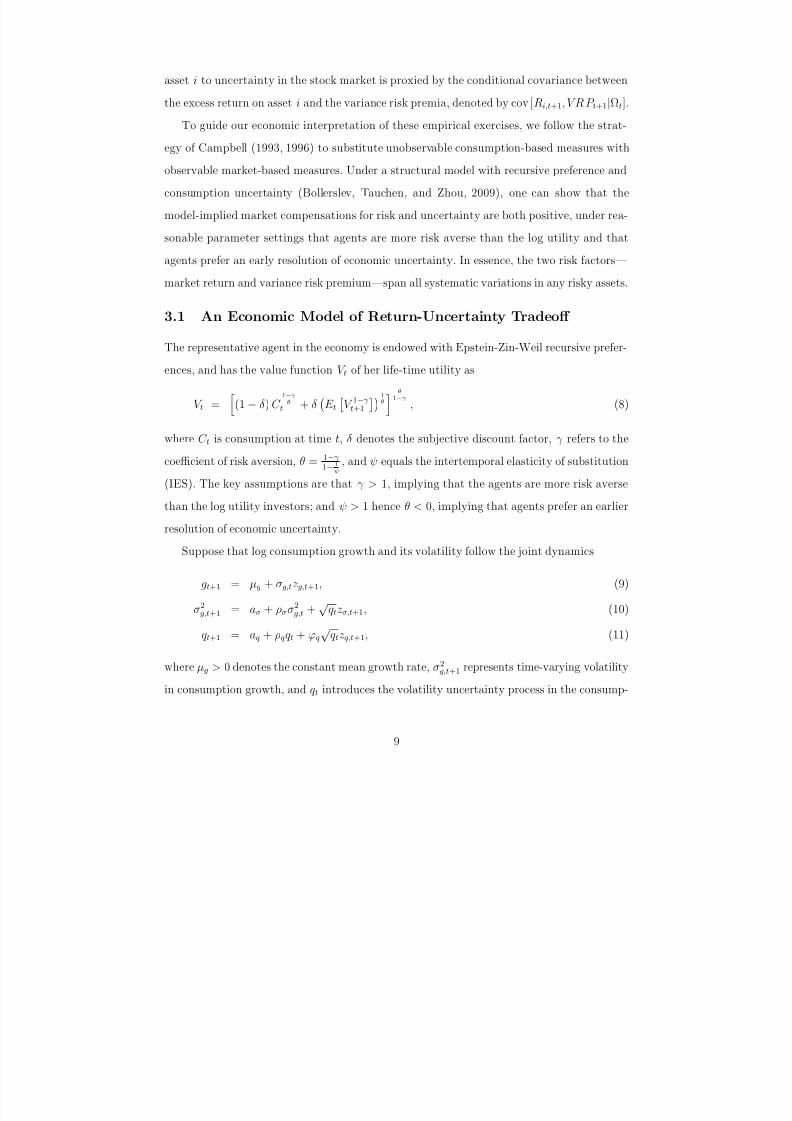
To guide our economic interpretation of these empirical exercises, we follow the strat-
egy of Campbell (1993, 1996) to substitute unobservable consumption-based measures withobservable market-based measures. Under a structural model with recursive preference and
consumption uncertainty (Bollerslev, Tauchen, and Zhou, 2009), one can show that the
model-implied market compensations for risk and uncertainty are both positive, under rea-
sonable parameter settings that agents are more risk averse than the log utility and that
agents prefer an early resolution of economic uncertainty. In essence, the two risk factors—
market return and variance risk premium—span all systematic variations in any risky assets.
3.1 An Economic Model of Return-Uncertainty Tradeoff
The representative agent in the economy is endowed with Epstein-Zin-Weil recursive prefer-
ences, and has the value function V t of her life-time utility as
V t =
(1 − δ) C 1−γθ
t + δ
E t
V 1−γ t+1
1θ
θ1−γ
, (8)
where C t is consumption at time t, δ denotes the subjective discount factor, γ refers to the
coefficient of risk aversion, θ = 1−γ 1− 1
ψ
, and ψ equals the intertemporal elasticity of substitution
(IES). The key assumptions are that γ > 1, implying that the agents are more risk averse
than the log utility investors; and ψ > 1 hence θ < 0, implying that agents prefer an earlier
resolution of economic uncertainty.
Suppose that log consumption growth and its volatility follow the joint dynamics
gt+1 = µg + σg,tzg,t+1, (9)
σ2g,t+1 = aσ + ρσσ2g,t + √qtzσ,t+1, (10)
qt+1 = aq + ρqqt + ϕq
√qtzq,t+1, (11)
where µg > 0 denotes the constant mean growth rate, σ2g,t+1 represents time-varying volatility
in consumption growth, and qt introduces the volatility uncertainty process in the consump-
9

7/31/2019 Risk Uncertainty and Return
http://slidepdf.com/reader/full/risk-uncertainty-and-return 13/75
tion growth process.7
Let wt denote the logarithm of the price-dividend or wealth-consumption ratio, of the
asset that pays the consumption endowment, C t+i∞i=1; and conjecture a solution for wt as
an affine function of the state variables, σ2
g,t and qt,
wt = A0 + Aσσ2g,t + Aqqt. (12)
One can solve for the coefficients A0, Aσ and Aq using the standard Campbell and Shiller
(1988) approximation rt+1 = κ0 + κ1wt+1 − wt + gt+1, where rt+1 is the return on the asset
that pays the consumption endowment flow. The restrictions that γ > 1 and ψ > 1, hence
θ < 0, imply that the impact coefficients associated with both volatility and uncertainty
state variables are negative; i.e., Aσ < 0 and Aq < 0. So if consumption risk and economic
uncertainty are high, the price-dividend ratio is low, hence risk premia are high.
Given the solution of price-dividend ratio, and assume that dividend equals consumption,
the model-implied premium of the market portfolio can be shown as
E [Rm,t+1|Ωt] = γσ2g,t + (1 − θ)κ2
1(A2qϕ2
q + A2σ)qt. (13)
The premium is composed of two separate terms. The first term, γσ 2g,t, is compensating for
the classic consumption risk as in a standard consumption-based CAPM model. The second
term, (1 − θ)κ21(A2
qϕ2q + A2
σ)qt, represents a true premium for variance risk or economic
uncertainty. The restrictions that γ > 1 and ψ > 1 implies that the uncertainty or variance
risk premium is always positive by construction.
The conditional variance of the time t to t + 1 market return, σ2m,t ≡ Vart(rt+1), can be
shown as σ2m,t = σ2
g,t + κ21
A2
σ + A2qϕ2
q
qt. The variance risk premium can be defined as the
difference between risk-neutral and objective expectations of the return variance,
8
V RP t ≡ EQ
σ2m,t+1|Ωt
− EP
σ2m,t+1|Ωt
≈ (θ − 1)κ1
Aσ + Aqκ2
1
A2
σ + A2qϕ2
q
ϕ2
q
qt.
7The parameters satisfy aσ > 0, aq > 0, |ρσ| < 1, |ρq| < 1, ϕq > 0; and zg,t, zσ,t and zq,t are iidNormal(0, 1) processes jointly independent with each other.
8The approximation comes from the fact that the model-implied risk-neutral conditional expectationcannot be computed in closed form, and a log-linear approximation is applied.
10

7/31/2019 Risk Uncertainty and Return
http://slidepdf.com/reader/full/risk-uncertainty-and-return 14/75
Moreover, provided that θ < 0, Aσ < 0, and Aq < 0, as would be implied by the agents’
preference of an earlier resolution of economic uncertainty, this difference between the risk-
neutral and objective expectations of return variances is guaranteed to be positive.
However, due to the measurement difficulty in consumption data and its volatility, wewill use market return volatility and variance risk premium to substitute fundamental risk
and uncertainty that are harder to pin down accurately (Campbell, 1993),
E [Rm,t+1|Ωt] = γσ2m,t +
(1 − θ − γ )κ21(A2
σ + A2qϕ2
q)
(θ − 1)κ1
Aσ + Aqκ2
1
A2
σ + A2qϕ2
q
ϕ2
q
V RP t . (14)
Therefore the risk-return trade-off identified by γ is always positive. However, the uncertainty-
return trade-off depends on the sign of (1−θ−γ ). Under typical preference parameter setting,
as in Bansal and Yaron (2004) and Bollerslev, Tauchen, and Zhou (2009), θ tends to be a
large negative number, and one always has (1 − θ − γ ) > 0. In other words, the model
implied uncertainty-return tradeoffs should always be positive.
Campbell (1993) shows that, in an intertemporal CAPM setting (Merton, 1973), the
appropriate choices for factors relevant in cross-sectional asset pricing tests should be the
current market return and any variables that have information about the future market
returns. Given the recent evidence that variance risk premium (VRP) possesses a significant
forecasting power for short-term market returns (see, e.g., Bollerslev, Tauchen, and Zhou,
2009, among others), it is natural to postulate the following cross-sectional asset pricing
implication along the lines of Campbell, Giglio, Polk, and Turley (2012):
E [Ri,t+1|Ωt] = A · cov[Ri,t+1, Rm,t+1|Ωt] + B · cov[Ri,t+1, ht+1|Ωt] , (15)
where the model implied coefficients A = γ > 0 and B = −θ/ψ > 0, and we approximate
the intertemporal hedging component ht with variance risk premium V RP t. The intuitionfor the positive slope coefficient B, is that investors dislike the reduced ability to hedge
against a deterioration in the investment opportunity captured by V RP t—which positively
predicts future market returns. Therefore investors require a higher return premium to hold
the assets or stocks that positively covary with V RP t (Campbell, 1996).
11

7/31/2019 Risk Uncertainty and Return
http://slidepdf.com/reader/full/risk-uncertainty-and-return 15/75
3.2 Calibrating Uncertainty-Return Tradeoff
To give some empirical guidance on how such a modeling framework with two risk drivers—
consumption risk and volatility uncertainty—can play out in empirically testing the time-
series and cross-sectional stock returns, we provide some calibration evidence based on the
model parameter settings used by Bollerslev, Tauchen, and Zhou (2009, or BTZ2009 for
short) focusing on equity return predictability and Zhou (2010) also considering bond return
and credit spread predictability. As shown in Table 1, consistent with the analytical charac-
terization above, the risk-return trade-off coefficient or A should be equal to the risk-aversion
coefficient, which is 10 or 2 under the two model parameter choices. On the other hand,
the uncertainty-return coefficient or B should be equal to 10.24 or 0.08, which is a highly
non-linear function of both the underlying preference and structural parameters. The model
implied uncertainty-return trade-off is positive.
More importantly, the positive relationship between variance risk premium and excess
market return is fairly robust. There are two key preference parameters—intertemporal
elasticity of substitution (IES) and risk aversion coefficient that may materially affect the
sign and magnitude of the return-uncertainty trade-off. However, as shown in the top two
panels of Figure 1, as long as IES—ψ is larger than one and risk aversion—γ is larger than
one, the model-implied linkage between return and uncertainty should remain positive.
In contrast, when agents prefer a late resolution of uncertainty or 0 < ψ < 1 (bottom left
panel), the model implied return-uncertainty trade-off swings between positive and negative
values with a bifurcation towards infinities near ψ = 0.5. Similarly, if agents are less risk
averse than log investor or 0 < γ < 1 (bottom right panel), the uncertainty-return trade-
off also swings between large positive and negative values near γ = 0.67. The empirical
implication is rather sharp—if we find that the exposures to variance risk premium are
positively priced in stock returns, it would be consistent with our assumptions that both
IES and risk aversion are larger than one—as sufficient conditions.
There is a long debate about whether the intertemporal elasticity of substitution or IES is
larger than one. As emphasized by Beeler and Campbell (2009), a high IES—around 1.5—is
12
7/31/2019 Risk Uncertainty and Return
http://slidepdf.com/reader/full/risk-uncertainty-and-return 16/75
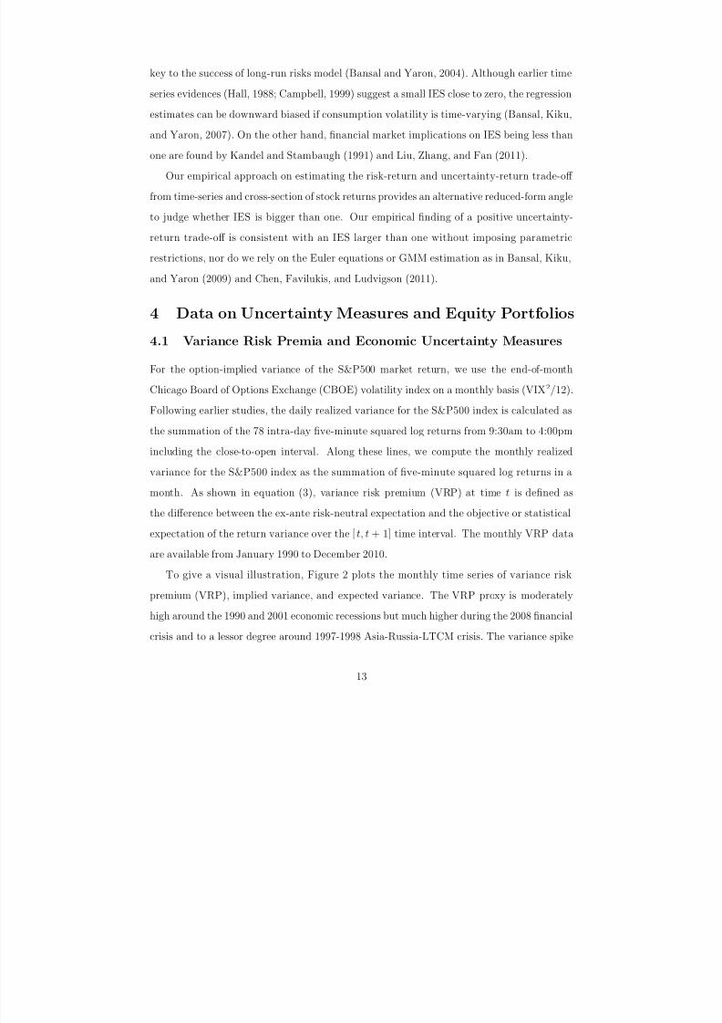
key to the success of long-run risks model (Bansal and Yaron, 2004). Although earlier time
series evidences (Hall, 1988; Campbell, 1999) suggest a small IES close to zero, the regression
estimates can be downward biased if consumption volatility is time-varying (Bansal, Kiku,
and Yaron, 2007). On the other hand, financial market implications on IES being less thanone are found by Kandel and Stambaugh (1991) and Liu, Zhang, and Fan (2011).
Our empirical approach on estimating the risk-return and uncertainty-return trade-off
from time-series and cross-section of stock returns provides an alternative reduced-form angle
to judge whether IES is bigger than one. Our empirical finding of a positive uncertainty-
return trade-off is consistent with an IES larger than one without imposing parametric
restrictions, nor do we rely on the Euler equations or GMM estimation as in Bansal, Kiku,
and Yaron (2009) and Chen, Favilukis, and Ludvigson (2011).
4 Data on Uncertainty Measures and Equity Portfolios
4.1 Variance Risk Premia and Economic Uncertainty Measures
For the option-implied variance of the S&P500 market return, we use the end-of-month
Chicago Board of Options Exchange (CBOE) volatility index on a monthly basis (VIX2/12).
Following earlier studies, the daily realized variance for the S&P500 index is calculated asthe summation of the 78 intra-day five-minute squared log returns from 9:30am to 4:00pm
including the close-to-open interval. Along these lines, we compute the monthly realized
variance for the S&P500 index as the summation of five-minute squared log returns in a
month. As shown in equation (3), variance risk premium (VRP) at time t is defined as
the difference between the ex-ante risk-neutral expectation and the objective or statistical
expectation of the return variance over the [t, t + 1] time interval. The monthly VRP data
are available from January 1990 to December 2010.
To give a visual illustration, Figure 2 plots the monthly time series of variance risk
premium (VRP), implied variance, and expected variance. The VRP proxy is moderately
high around the 1990 and 2001 economic recessions but much higher during the 2008 financial
crisis and to a lessor degree around 1997-1998 Asia-Russia-LTCM crisis. The variance spike
13

7/31/2019 Risk Uncertainty and Return
http://slidepdf.com/reader/full/risk-uncertainty-and-return 17/75
during October 2008 already surpasses the initial shock of the Great Depression in October
1929. The huge run-up of VRP in the fourth quarter of 2008 leads the equity market bottom
reached in March 2009. The sample mean of VRP is 18.75 (in percentages squared, monthly
basis), with a standard deviation of 22.15. Notice that the extraordinary skewness (3.81)and kurtosis (27.46) signal a highly non-Gaussian process for VRP.
According to our model in Section 3, VRP can be viewed as a proxy for uncertainty. To
test whether VRP is in fact associated with alternative measures of uncertainty, we generate
some proxies for financial and economic uncertainty. We obtain monthly values of the U.S.
industrial production index from G.17 database of the Federal Reserve Board and monthly
values of the Chicago Fed National Activity Index (CFNAI) from the Federal Reserve Bank
of Chicago for the period January 1990 – December 2010.9 We use a GARCH(1,1) model of
Bollerslev (1986) to estimate the conditional variance of the growth rate of industrial produc-
tion and the conditional variance of the CFNAI index. These two measures can be viewed
as macroeconomic uncertainty. The sample correlation between VRP and economic uncer-
tainty variables is positive and significant; sample correlation is 33.20% with the variance of
output growth and 31.82% with the variance of CFNAI index.
Our second set of uncertainty measures is based on the downside risk of financial institu-
tions obtained from the left tail of the time-series and cross-sectional distribution of financial
firms’ returns. Specifically, we obtain monthly returns for financial firms (6000 ≤ SIC code
≤ 6999) for the sample period January 1990 to December 2010. Then, the 1% nonparametric
Value-at-Risk (VaR) measure in a given month is measured as the cut-off point for the lower
one percentile of the monthly returns on financial firms.10 For each month, we determine
the one percentile of the cross-section of returns on financial firms, and obtain an aggre-
gate 1% VaR measure of the financial system for the period 1990-2010. In addition to the
9The CFNAI is a monthly index that determines increases and decreases in economic activity and isdesigned to assess overall economic activity and related inflationary pressure. It is a weighted average of 85 existing monthly indicators of national economic activity, and is constructed to have an average value of zero and a standard deviation of one. Since economic activity tends toward a trend growth rate over time,a positive index reading corresponds to growth above trend and a negative index reading corresponds togrowth below trend.
10Assuming that we have 900 financial firms in month t, the nonparametric measure of 1% VaR is the 9thlowest observation in the cross-section of monthly returns.
14

7/31/2019 Risk Uncertainty and Return
http://slidepdf.com/reader/full/risk-uncertainty-and-return 18/75
cross-sectional distribution, we use the time-series daily return distribution to estimate 1%
VaR of the financial system. For each month from January 1990 to December 2010, we first
determine the lowest daily returns on financial institutions over the past 1 to 12 months. The
catastrophic risk of financial institutions is then computed by taking the average of theselowest daily returns obtained from alternative measurement windows. The estimation win-
dows are fixed at 1 to 12 months, and each fixed estimation window is updated on a monthly
basis. These two downside risk measures can be viewed as a proxy for uncertainty in the
financial sector. The sample correlations between VRP and financial uncertainty variables
are positive and significant: 47.37% with the cross-sectional VaR measure and 37.01% with
the time-series VaR measure.
The third uncertainty variable is related to the health of the financial sector proxied by the
credit default swap (CDS) index. We download the monthly CDS data from Bloomberg. For
the sample period January 2004 – December 2010, we obtain monthly CDS data for Bank of
America (BOA), Citigroup (CICN), Goldman Sachs (GS), JP Morgan (JPM), Morgan Stan-
ley (MS), Wells Fargo (WFC), and American Express (AXP). Then, we standardized all
CDS data to have zero mean and unit standard deviation. Finally, we formed the standard-
ized CDS index (EWCDS) based on the equal-weighted average of standardized CDS values
for the 7 major financial firms. For the common sample period 2004-2010, the correlation
between VRP and EWCDS is positive, 42.99%, and highly significant.
The last uncertainty variable is based on the aggregate measure of investors’ disagree-
ment about individual stocks trading at NYSE, AMEX, and NASDAQ. Following Diether,
Malloy, and Scherbina (2002), we use dispersion in analysts’ earnings forecasts as a proxy
for divergence of opinion. It is likely that investors partly form their expectations about a
particular stock based on the analysts’ earnings forecasts. If all analysts are in agreement
about expected returns, uncertainty is likely to be low. However, if analysts provide very
different estimates, investors are likely to be unclear about future returns, and uncertainty
is high. The sample correlation between VRP and the aggregate measure of dispersion is
about 14.92%. Overall, these results indicate that the variance risk premia is strongly and
positively correlated with all measures of uncertainty considered here. Hence, VRP can be
15

7/31/2019 Risk Uncertainty and Return
http://slidepdf.com/reader/full/risk-uncertainty-and-return 19/75
viewed as a sound proxy for financial and economic uncertainty.
4.2 Equity Portfolios
We use the monthly excess returns on the value-weighted aggregate market portfolio andthe monthly excess returns on the 10 value-weighted size, book-to-market, and industry
portfolios. The aggregate market portfolio is represented by the value-weighted NYSE-
AMEX-NASDAQ index. Excess returns on portfolios are obtained by subtracting the returns
on the one-month Treasury bill from the raw returns on equity portfolios. The data are
obtained from Kenneth French’s online data library.11 We use the longest common sample
period available, from January 1990 to December 2010, yielding a total of 252 monthly
observations.
Table I of the internet appendix presents the monthly raw return and CAPM Alpha dif-
ferences between high-return (long) and low-return (short) equity portfolios. The results are
reported for the size, book-to-market (BM), and industry portfolios for the period January
1990 – December 2010.12 The OLS t-statistics are reported in parentheses. The Newey and
West (1987) t-statistics are given in square brackets.
For the ten size portfolios, “Small” (Decile 1) is the portfolio of stocks with the smallest
market capitalization and “Big” (Decile 10) is the portfolio of stocks with the biggest market
capitalization. For the 1990-2010 period, the average return difference between the Small and
Big portfolios is 0.40% per month with the OLS t-statistic of 1.22 and the Newey-West (1987)
t-statistic of 1.13, implying that small stocks on average do not generate higher returns than
big stocks. In addition to the average raw returns, Table I of the internet appendix presents
the intercept (CAPM alpha) from the regression of Small-Big portfolio return difference on
a constant and the excess market return. The CAPM Alpha (or abnormal return) for the
long-short size portfolio is 0.35% per month with the OLS t-statistic of 1.06 and the Newey-
West t-statistic of 0.98. This economically and statistically insignificant Alpha indicates that
the static CAPM does explain the size effect for the 1990-2010 period.
11http://mba.tuck.dartmouth.edu/pages/faculty/ken.french/data library.html12Since the monthly data on variance risk premia (VRP) start in January 1990, our empirical analyses
with equity portfolios and VRP are based on the sample period January 1990 - December 2010.
16

7/31/2019 Risk Uncertainty and Return
http://slidepdf.com/reader/full/risk-uncertainty-and-return 20/75
For the ten book-to-market portfolios, “Growth” is the portfolio of stocks with the lowest
book-to-market ratios and “Value” is the portfolio of stocks with the highest book-to-market
ratios. For the sample period January 1990 – December 2010, the average return difference
between the Value and Growth portfolios is economically and statistically insignificant; 0.29%per month with the OLS t-statistic of 0.92 and the Newey-West t-statistic of 0.79, implying
that value stocks on average do not generate higher returns than growth stocks. Similar to
our findings for the size portfolios, the unconditional CAPM can explain the value premium
for the 1990-2010 period; the CAPM Alpha (or abnormal return) for the long-short book-to-
market portfolio is only 0.28% per month with the OLS t-statistic of 0.86 and the Newey-West
t-statistic of 0.71.
Interestingly, industry effects in the U.S. equity market are economically and statistically
strong over the past two decades, although size and value premiums are not. The average
raw and risk-adjusted return differences between the high-return and low-return industry
portfolios are significant for the sample period 1990-2010. The high-return and low-return
portfolios of 48 and 49 industries generate highly significant return differences, 30 and 38
industry portfolios generate marginally significant return differences, whereas the average
return differences and Alphas for the high-return and low-return portfolios of 10 and 17
industries are insignificant. Specifically, for 30-, 48- and 49-industry portfolios of Kenneth
French, “Coal” industry has the highest average monthly return, whereas “Other” industry
has the lowest return, yielding an average raw and risk-adjusted return differences of 1.54%
to 1.79% per month and statistically significant. The static CAPM cannot explain these
economically and statistically strong industry effects either.
Earlier studies starting with Fama and French (1992, 1993) provide evidence for the
significant size and value premiums for the post-1963 period. Some readers may find the
insignificant size and value premiums for the 1990-2010 period controversial. Hence, in
internet appendix (Section A), we examine the significance of size and book-to-market effects
for the longest sample period July 1926 – December 2010 and the subsample period July
1963 – December 2010. The results indicate significant raw return difference between the
Value and Growth portfolios for both sample periods and significant risk-adjusted return
17

7/31/2019 Risk Uncertainty and Return
http://slidepdf.com/reader/full/risk-uncertainty-and-return 21/75
difference (Alpha) only for the post-1963 period. Consistent with the findings of earlier
studies, we find significant raw return difference between the Small and Big stock portfolios
for the 1926-2010 period, which becomes very weak for the post-1963 period. The CAPM
Alpha (or abnormal return) for the long-short size portfolio is economically and statisticallyinsignificant for both sample periods.
5 Estimation Methodology
Following Bali (2008) and Bali and Engle (2010), our estimation approach proceeds in steps.
1) We take out any autoregressive elements in returns and VRP and estimate univariate
GARCH models for all returns and VRP.
2) We construct standardized returns and compute bivariate DCC estimates of the cor-
relations between each portfolio and the market and between each portfolio and VRP
using the bivariate likelihood function.
3) We estimate the expected return equation as a panel with the conditional covariances
as regressors. The error covariance matrix specified as seemingly unrelated regression
(SUR). The panel estimation methodology with SUR takes into account heteroskedas-ticity and autocorrelation as well as contemporaneous cross-correlations in the error
terms.
The following subsections provide details about the estimation of time-varying covariances
and the estimation of time-series and cross-sectional relation between expected returns and
risk and uncertainty.
5.1 Estimating Time-Varying Conditional Covariances
We estimate the conditional covariance between excess returns on equity portfolio i and
the market portfolio m based on the mean-reverting dynamic conditional correlation (DCC)
model:
Ri,t+1 = αi0 + αi
1Ri,t + εi,t+1 (16)
18

7/31/2019 Risk Uncertainty and Return
http://slidepdf.com/reader/full/risk-uncertainty-and-return 22/75
Rm,t+1 = αm0 + αm
1 Rm,t + εm,t+1 (17)
E t
ε2i,t+1
≡ σ2i,t+1 = βi
0 + βi1ε2
i,t + βi2σ2
i,t (18)
E t ε2m,t+1 ≡
σ2m,t+1 = βm
0 + βm1 ε2
m,t + βm2 σ2
m,t (19)
E t [εi,t+1εm,t+1] ≡ σim,t+1 = ρim,t+1 · σi,t+1 · σm,t+1 (20)
ρim,t+1 =qim,t+1√
qii,t+1 · qmm,t+1, qim,t+1 = ρim + a1 · (εi,t · εm,t − ρim) + a2 · (qim,t − ρim) (21)
where Ri,t+1 and Rm,t+1 denote the time (t+1) excess return on equity portfolio i and the mar-
ket portfolio m over a risk-free rate, respectively, and E t [·] denotes the expectation operator
conditional on time t information. σ2i,t+1 is the time-t expected conditional variance of Ri,t+1,
σ2m,t+1 is the time-t expected conditional variance of Rm,t+1, and σim,t+1 is the time-t expected
conditional covariance between Ri,t+1 and Rm,t+1. ρim,t+1 = qim,t+1/√
qii,t+1 · qmm,t+1 is the
time-t expected conditional correlation between Ri,t+1 and Rm,t+1, and ρim is the uncondi-
tional correlation. To ease the parameter convergence, we use correlation targeting assuming
that the time-varying correlations mean reverts to the sample correlations ρim.
We estimate the conditional covariance between each equity portfolio i and the variance
risk premia V RP , σi,V RP , using an analogous DCC model:
Ri,t+1 = αi0 + αi
1Ri,t + εi,t+1 (22)
V RP t+1 = αV RP 0 + αV RP
1 V RP t + εV RP,t+1 (23)
E t
ε2i,t+1
≡ σ2i,t+1 = βi
0 + βi1ε2
i,t + βi2σ2
i,t (24)
E t
ε2V RP,t+1
≡ σ2V RP,t+1 = βV RP
0 + βV RP 1 ε2
V RP,t + βV RP 2 σ2
V RP,t (25)
E t [εi,t+1εV RP,t+1] ≡ σi,V RP,t+1 = ρi,V RP,t+1 · σi,t+1 · σV RP,t+1 (26)
ρi,V RP,t+1 =qi,V RP,t+1√
qii,t+1 · qV RP,t+1,
qi,V RP,t+1 = ρi,V RP + a1 · (εi,t · εV RP,t − ρi,V RP ) + a2 · (qi,V RP,t − ρi,V RP ) (27)
where σi,V RP,t+1 is the time-t expected conditional covariance between Ri,t+1 and V RP t+1.
ρi,V RP,t+1 is the time-t expected conditional correlation between Ri,t+1 and V RP t+1. We use
19

7/31/2019 Risk Uncertainty and Return
http://slidepdf.com/reader/full/risk-uncertainty-and-return 23/75
the same DCC model to estimate the conditional covariance between the market portfolio
m and the variance risk premia V RP , σm,V RP .13
We estimate the conditional covariances of each equity portfolio with the market portfolio
and with V RP using the maximum likelihood method described in the internet appendix(Section B). Then, as discussed in the following section, we estimate the time-series and
cross-sectional relation between expected return and risk and uncertainty as a panel with
the conditional covariances as regressors.
5.2 Estimating Risk-Uncertainty-Return Tradeoff
Given the conditional covariances, we estimate the portfolio-specific intercepts and the com-
mon slope estimates from the following panel regression:
Ri,t+1 = αi + A · Covt (Ri,t+1, Rm,t+1) + B · Covt (Ri,t+1, V R P t+1) + εi,t+1 (28)
Rm,t+1 = αm + A · V art (Rm,t+1) + B · Covt (Rm,t+1, V R P t+1) + εm,t+1 (29)
where Covt (Ri,t+1, Rm,t+1) is the time-t expected conditional covariance between the ex-
cess return on portfolio i (Ri,t+1) and the excess return on the market portfolio (Rm,t+1),
Covt (Ri,t+1, V R P t+1) is the time-t expected conditional covariance between the excess re-
turn on portfolio i and the variance risk premia (V RP t+1), Covt (Rm,t+1, V R P t+1) is the
time-t expected conditional covariance between the excess return on the market portfolio m
and the variance risk premia (V RP t+1), and V art (Rm,t+1) is the time-t expected conditional
variance of excess returns on the market portfolio.
We estimate the system of equations in (28)-(29) using a weighted least square method
that allows us to place constraints on coefficients across equations. We compute the t-
statistics of the parameter estimates accounting for heteroskedasticity and autocorrelation
as well as contemporaneous cross-correlations in the errors from different equations. The es-
timation methodology can be regarded as an extension of the seemingly unrelated regression
13We assume that the excess returns on equity portfolios and the market portfolio as well as the variancerisk premia follow an autoregressive of order one, AR(1) process, given in equations (16), (17), and (23). Atan earlier stage of the study, we consider alternative specifications of the conditional mean. More specifically,the excess returns are assumed to follow a moving average of order one, MA(1) process, ARMA(1,1) process,and a constant. Our main findings are not sensitive to the choice of the conditional mean specification.
20

7/31/2019 Risk Uncertainty and Return
http://slidepdf.com/reader/full/risk-uncertainty-and-return 24/75
(SUR) method, the details of which are in the internet appendix (Section C).
6 Empirical Results
In this section we first present results from the 10 decile portfolios of size, book-to-market,
and industry. Second, we discuss the economic significance of risk and uncertainty compensa-
tions and the underlying economic intuition. Finally, we compare the relative performances
of conditional CAPM and ICAPM with both risk and uncertainty.
6.1 Ten Decile Portfolios of Size, Book-to-Market, and Industry
The common slopes and the intercepts are estimated using the monthly excess returns on
the 10 value-weighted size, book-to-market, and industry portfolios for the sample period
January 1990 to December 2010. The aggregate stock market portfolio is measured by
the value-weighted CRSP index. Table 2 reports the common slope estimates (A, B), the
abnormal returns or conditional alphas for each equity portfolio (αi) and the market portfolio
(αm), and the t-statistics of the parameter estimates. The last two rows, respectively, show
the Wald statistics; Wald1 from testing the joint hypothesis H 0 : α1 = ... = α10 = αm = 0,
and Wald2 from testing the equality of conditional alphas for high-return and low-return
portfolios (Small vs. Big; Value vs. Growth; and HiTec vs. Telcm). The p-values of Wald1
and Wald2 statistics are given in square brackets.
The risk aversion coefficient is estimated to be positive and highly significant for all
equity portfolios: A = 3.96 with the t-statistic of 3.12 for the size portfolios, A = 2.51 with
the t-statistic of 2.53 for the book-to-market portfolios, and A = 3.41 with the t-statistic
of 2.35 for the industry portfolios.14 These results imply a positive and significant relation
between expected return and market risk.15
Consistent with our theoretical model, theuncertainty aversion coefficient is also estimated to be positive and highly significant for all
14Our risk aversion estimates ranging from 2.51 to 3.41 are very similar to the median level of risk aversion,2.52, identified by Bekaert, Engstrom, and Xing (2009) in a different model.
15Although the literature is inconclusive on the direction and significance of a risk-return tradeoff, somestudies do provide evidence supporting a positive and significant relation between expected return andrisk (e.g., Bollerslev, Engle, and Wooldridge (1988), Ghysels, Santa-Clara, and Valkanov (2005), Guo andWhitelaw (2006), Guo and Savickas (2006), Lundblad (2007), Bali (2008), and Bali and Engle (2010)).
21
7/31/2019 Risk Uncertainty and Return
http://slidepdf.com/reader/full/risk-uncertainty-and-return 25/75
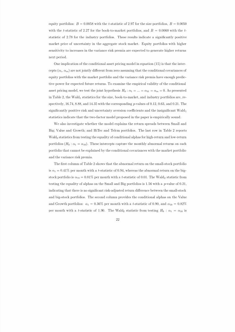
equity portfolios: B = 0.0058 with the t-statistic of 2.97 for the size portfolios, B = 0.0050
with the t-statistic of 2.27 for the book-to-market portfolios, and B = 0.0060 with the t-
statistic of 2.78 for the industry portfolios. These results indicate a significantly positive
market price of uncertainty in the aggregate stock market. Equity portfolios with highersensitivity to increases in the variance risk premia are expected to generate higher returns
next period.
One implication of the conditional asset pricing model in equation (15) is that the inter-
cepts (αi, αm) are not jointly different from zero assuming that the conditional covariances of
equity portfolios with the market portfolio and the variance risk premia have enough predic-
tive power for expected future returns. To examine the empirical validity of the conditional
asset pricing model, we test the joint hypothesis H 0 : α1 = ... = α10 = αm = 0. As presented
in Table 2, the Wald1 statistics for the size, book-to-market, and industry portfolios are, re-
spectively, 16.74, 8.88, and 14.35 with the corresponding p-values of 0.12, 0.63, and 0.21. The
significantly positive risk and uncertainty aversion coefficients and the insignificant Wald1
statistics indicate that the two-factor model proposed in the paper is empirically sound.
We also investigate whether the model explains the return spreads between Small and
Big; Value and Growth; and HiTec and Telcm portfolios. The last row in Table 2 reports
Wald2 statistics from testing the equality of conditional alphas for high-return and low-return
portfolios (H 0 : α1 = α10). These intercepts capture the monthly abnormal returns on each
portfolio that cannot be explained by the conditional covariances with the market portfolio
and the variance risk premia.
The first column of Table 2 shows that the abnormal return on the small-stock portfolio
is α1 = 0.41% per month with a t-statistic of 0.94, whereas the abnormal return on the big-
stock portfolio is α10 = 0.01% per month with a t-statistic of 0.01. The Wald2 statistic from
testing the equality of alphas on the Small and Big portfolios is 1.56 with a p-value of 0.21,
indicating that there is no significant risk-adjusted return difference between the small-stock
and big-stock portfolios. The second column provides the conditional alphas on the Value
and Growth portfolios: α1 = 0.36% per month with a t-statistic of 0.90, and α10 = 0.82%
per month with a t-statistic of 1.90. The Wald2 statistic from testing H 0 : α1 = α10 is
22

7/31/2019 Risk Uncertainty and Return
http://slidepdf.com/reader/full/risk-uncertainty-and-return 26/75
1.79 with a p-value of 0.18, implying that the conditional asset pricing model explains the
value premium, i.e., the risk-adjusted return difference between value and growth stocks is
statistically insignificant. The last column shows that the conditional alphas on HiTec and
Telcm portfolios are, respectively, 0.26% and -0.05% per month, generating a risk-adjustedreturn spread of 31 basis points per month. As reported in the last row, the Wald2 statistic
from testing the significance of this return spread is 0.40 with a p-value of 0.53, yielding
insignificant industry effect over the sample period 1990-2010.
The differences in conditional alphas are both economically and statistically insignificant,
indicating that the two-factor model proposed in the paper provides both statistical and
economic success in explaining stock market anomalies. Overall, the DCC-based conditional
covariances capture the time-series and cross-sectional variation in returns on size, book-
to-market, and industry portfolios because the essential tests of the conditional ICAPM
are passed: (i) significantly positive risk-return and uncertainty-return tradeoffs; (ii) the
conditional alphas are jointly zero; and (iii) the conditional alphas for high-return and low-
return portfolios are not statistically different from each other.16
6.2 Economic Significance of Uncertainty-Return Tradeoff
In this section, we test whether the risk-return (A) and uncertainty-return (B) coefficients
are sensible and whether the uncertainty measure is associated with macroeconomic state
variables.
Specifically, we rely on equation (29) and compute the expected excess return on the
market portfolio based on the estimated prices of risk and uncertainty as well as the sample
averages of the conditional covariance measures:
E t [Rm,t+1] = αm + A · V art (Rm,t+1) + B · Covt (Rm,t+1, V R P t+1) (30)
where αm = 0.0008, A = 3.96, and B = 0.0058 for the 10 size portfolios; αm = 0.0032,
A = 2.51, and B = 0.0050 for the 10 book-to-market portfolios; and αm = 0.0019, A =
16As discussed in Section D of the internet appendix, we estimate the DCC-based conditional covariancesusing the Asymmetric GARCH model of Glosten, Jagannathan, and Runkle (1993). Table II of the internetappendix shows that our main findings from the Asymmetric GARCH model are very similar to thosereported in Table 2.
23

7/31/2019 Risk Uncertainty and Return
http://slidepdf.com/reader/full/risk-uncertainty-and-return 27/75
3.41, and B = 0.0060 for the 10 industry portfolios (see Table 2). The sample averages
of V art (Rm,t+1) and Covt (Rm,t+1, V R P t+1) are 0.002187 and -0.7026, respectively.17 These
values produce E t [Rm,t+1] = 0.54% per month when the parameters are estimated using
the 10 size portfolios, E t [Rm,t+1] = 0.52% per month when the parameters are estimatedusing the 10 book-to-market portfolios, and E t [Rm,t+1] = 0.51% when the parameters are
estimated using the 10 industry portfolios.
To evaluate the performance of our model with risk and uncertainty, we calculate the
sample average of excess returns on the market portfolio, which is a standard benchmark
for the market risk premium. The sample average of Rm,t+1 is found to be 0.52% per month
for the period January 1990 – December 2010, indicating that the estimated market risk
premiums of 0.51% – 0.54% are very close to the benchmark. This again shows outstanding
performance of the two-factor model introduced in the paper.
To further appreciate the economics behind the apparent connection between the variance
risk premium (VRP) and the time-series and cross-sectional variations in expected stock
returns, Figure 3 plots the VRP together with the quarterly growth rate in GDP. As seen
from the figure, there is a tendency for VRP to rise in the quarter before a decline in GDP,
while it typically narrows ahead of an increase in GDP. Indeed, the sample correlation equals
-0.17 between lag VRP and current GDP (as first reported in Bollerslev and Zhou, 2007).
In other words, VRP as a proxy for economic uncertainty does seem to negatively relate to
future macroeconomic performance.
Thus, not only the difference between the implied and expected variances positively
covaries with stock returns, it also covaries negatively with future growth rates in GDP.
Intuitively, when VRP is high (low), it generally signals a high (low) degree of aggregate
economic uncertainty. Consequently agents tend to simultaneously cut (increase) their con-
sumption and investment expenditures and shift their portfolios from more (less) to less
(more) risky assets. This in turn results in a rise (decrease) in expected excess returns for
stock portfolios that covaries more (less) with the macroeconomic uncertainty, as proxied by
17The negative value for the conditional covariance of the market return with the VRP factor is consistentwith our theoretical model and the negative contemporaneous correlation between the market return andthe VRP factor reported by Bollerslev, Tauchen, and Zhou (2009).
24

7/31/2019 Risk Uncertainty and Return
http://slidepdf.com/reader/full/risk-uncertainty-and-return 28/75
VRP. In essence, our finding of a positive significant relation between economic uncertainty
measure and stock expected returns, is consistent with our model’s setting where agents
prefer an earlier resolution of uncertainty. Therefore economic uncertainty carries a positive
premium, and heightened VRP does signal the worsening of macroeconomic fundamentals.
6.3 Relative Performance of Conditional ICAPM with Uncertainty
We now assess the relative performance of the newly proposed model in predicting the cross-
section of expected returns on equity portfolios. Specifically, we test whether the conditional
ICAPM with the market and uncertainty factors outperforms the conditional CAPM with
the market factor in terms of statistical fit. The goodness of fit of an asset pricing model
describes how well it fits a set of realized return observations. Measures of goodness of fit
typically summarize the discrepancy between observed values and the values expected under
the model in question. Hence, we focus on the cross-section of realized average returns on
equity portfolios (as a benchmark) and the portfolios’ expected returns implied by the two
competing models.
Using equation (28), we compute the expected excess return on equity portfolios based on
the estimated prices of risk and uncertainty (A, B) and the sample averages of the conditional
covariance measures, Covt (Ri,t+1, Rm,t+1) and Covt (Ri,t+1, V R P t+1):
E t [Ri,t+1] = αi + A · Covt (Ri,t+1, Rm,t+1) + B · Covt (Ri,t+1, V R P t+1) . (31)
Table 3 presents the realized monthly average excess returns on the size, book-to-market,
and industry portfolios and the cross-section of expected excess returns generated by the
Conditional CAPM and the Conditional ICAPM models. Clearly the newly proposed model
with risk and uncertainty provides much more accurate estimates of expected returns on the
size, book-to-market, and industry portfolios. Especially for the size and industry portfolios,
expected returns implied by the Conditional ICAPM with the market and VRP factors are
almost identical to the realized average returns. The last row in Table 3 reports the Mean
Absolute Percentage Errors (MAPE) for the two competing models:
MAPE =|Realized − Expected|
Expected, (32)
25

7/31/2019 Risk Uncertainty and Return
http://slidepdf.com/reader/full/risk-uncertainty-and-return 29/75
where “Realized” is the realized monthly average excess return on each equity portfolio and
“Expected” is the expected excess return implied by equation (31). For the conditional
CAPM with the market factor, MAPE equals 5.20% for the size portfolios, 5.37% for the
book-to-market portfolios, and 6.32% for the industry portfolios. Accounting for the variancerisk premium improves the cross-sectional fitting significantly: MAPE reduces to 0.61% for
the size portfolios, 1.66% for the book-to-market portfolios, and 0.55% for the industry
portfolios.
Figure 4 provides a visual depiction of the realized and expected returns for the size, book-
to-market, and industry portfolios. It is clear that our conditional ICAPM with uncertainty
nails down the realized returns of the size, book-to-market, and industrial portfolios, while
the conditional CAPM systematically over-predicts these portfolio returns. Overall, the
results indicate superior performance of the conditional asset pricing model introduced in
the paper.
7 Robustness Check
In this section we first examine whether the model’s performance changes when we use
a larger cross-section of equity portfolios. Second, we provide robustness analysis when
controlling for popular macroeconomic and financial variables. Third, we provide results
from individual stocks. Finally, we test whether the predictive power of the variance risk
premia is subsumed by the market illiquidity and/or credit risk.
7.1 Results from Larger Cross-Section of Industry Portfolios
Given the positive risk-return and positive uncertainty-return coefficient estimates from the
three data sets and the success of the conditional asset pricing model in explaining theindustry, size, and value premia, we now examine how the model performs when we use a
larger cross-section of equity portfolios.
The robustness of our findings is investigated using the monthly excess returns on the
value-weighted 17-, 30-, 38-, 48-, and 49-industry portfolios for the sample period January
26

7/31/2019 Risk Uncertainty and Return
http://slidepdf.com/reader/full/risk-uncertainty-and-return 30/75
1990 – December 2010. Table 4 reports the common slope estimates (A, B), their t-statistics
in parentheses, and the Wald1 and Wald2 statistics along with their p-values in square
brackets. For the industry portfolios, the risk aversion coefficients (A) are estimated to
be positive, in the range of 2.20 to 2.78, and highly significant with the t-statistics rangingfrom 2.31 to 3.34. Consistent with our earlier findings from the 10 size, 10 book-to-market,
and 10 industry portfolios, the results from the larger cross-section of industry portfolios (17
to 49) imply a positive and significant relation between expected return and market risk.
Again similar to our findings from 10 decile portfolios, the uncertainty aversion coefficients
are estimated to be positive, in the range of 0.0036 to 0.0041, and highly significant with
the t-statistics ranging from 2.44 to 4.21. These results provide evidence for a significantly
positive market price of uncertainty and show that assets with higher correlation with the
variance risk premia generate higher returns next month.
Not surprisingly, the Wald1 statistics for all industry portfolios have p-values in the range
of 0.20 to 0.75, indicating that the two-factor asset pricing model can explain the time-series
and cross-sectional variation in larger number of equity portfolios. The last row shows that
the Wald2 statistics from testing the equality of conditional alphas on the high-return and
low-return industry portfolios have p-values ranging from 0.44 to 0.80, implying that there
is no significant risk-adjusted return difference between the extreme portfolios of 17, 30,
38, 48, and 49 industries. The differences in conditional alphas are both economically and
statistically insignificant, showing that the two-factor model introduced in the paper provides
success in explaining industry effects.
7.2 Controlling for Macroeconomic Variables
A series of papers argue that the stock market can be predicted by financial and/or macroeco-
nomic variables associated with business cycle fluctuations. The commonly chosen variables
include default spread (DEF), term spread (TERM), dividend price ratio (DIV), and the
de-trended riskless rate or the relative T-bill rate (RREL).18 We define DEF as the difference
18See, e.g., Campbell (1987), Fama and French (1989), and Ferson and Harvey (1991) who test thepredictive power of these variables for expected stock returns.
27

7/31/2019 Risk Uncertainty and Return
http://slidepdf.com/reader/full/risk-uncertainty-and-return 31/75
between the yields on BAA- and AAA-rated corporate bonds, and TERM as the difference
between the yields on the 10-year Treasury bond and the 3-month Treasury bill. RREL is
defined as the difference between 3-month T-bill rate and its 12-month backward moving
average.19
We obtain the aggregate dividend yield using the CRSP value-weighted indexreturn with and without dividends based on the formula given in Fama and French (1988).
In addition to these financial variables, we use some fundamental variables affecting the state
of the U.S. economy: Monthly inflation rate based on the U.S. Consumer Price Index (INF);
Monthly growth rate of the U.S. industrial production (IP) obtained from the G.17 database
of the Federal Reserve Board; and Monthly US unemployment rate (UNEMP) obtained from
the Bureau of Labor Statistics.
According to Merton’s (1973) ICAPM, state variables that are correlated with changes
in consumption and investment opportunities are priced in capital markets in the sense that
an asset’s covariance with those state variables affects its expected returns. Merton (1973)
also indicates that securities affected by such state variables (or systematic risk factors)
should earn risk premia in a risk-averse economy. Macroeconomic variables used in the
literature are excellent candidates for these systematic risk factors because innovations in
macroeconomic variables can generate global impact on firm’s fundamentals, such as their
cash flows, risk-adjusted discount factors, and/or investment opportunities. Following the
existing literature, we use the aforementioned financial and macroeconomic variables as
proxies for state variables capturing shifts in the investment opportunity set.
We now investigate whether incorporating these variables into the predictive regressions
affects the significance of the market prices of risk and uncertainty. Specifically, we estimate
the portfolio-specific intercepts and the common slope coefficients from the following panel
regression:
Ri,t+1 = αi + A · Covt (Ri,t+1, Rm,t+1) + B · Covt (Ri,t+1, V R P t+1) + λ · X t + εi,t+1
Rm,t+1 = αm + A · V art (Rm,t+1) + B · Covt (Rm,t+1, V R P t+1) + λ · X t + εm,t+1
where X t denotes a vector of lagged control variables; default spread (DEF), term spread
19The monthly data on 10-year T-bond yields, 3-month T-bill rates, BAA- and AAA-rated corporate bondyields are available from the Federal Reserve statistics release website.
28

7/31/2019 Risk Uncertainty and Return
http://slidepdf.com/reader/full/risk-uncertainty-and-return 32/75
(TERM), relative T-bill rate (RREL), aggregate dividend yield (DIV), inflation rate (INF),
growth rate of industrial production (IP), and unemployment rate (UNEMP). The common
slope coefficients (A, B, and λ) and their t-statistics are estimated using the monthly excess
returns on the market portfolio and the ten size, book-to-market, and industry portfolios.As presented in Table 5, after controlling for a wide variety of financial and macroe-
conomic variables, our main findings remain intact for all equity portfolios. The common
slope estimates on the conditional covariances of equity portfolios with the market factor
(A) remain positive and highly significant, indicating a positive and significant relation be-
tween expected return and market risk. Similar to our earlier findings, the common slopes
on the conditional covariances of equity portfolios with the uncertainty factor (B) remain
significantly positive as well, showing that assets with higher correlation with the variance
risk premium generate higher returns next month. Among the control variables, the growth
rate of industrial production is the only variable predicting future returns on equity port-
folios; λIP turns out to be positive and significant—especially for the industry portfolios.
The positive relation between expected stock returns and innovations in output makes eco-
nomic sense. Increases in real economic activity (proxied by the growth rate of industrial
production) increase investors’ expectations of future growth. Overall, the results in Table
5 indicate that after controlling for variables associated with business conditions, the time-
varying exposures of equity portfolios to the market and uncertainty factors carry positive
risk premiums.20
7.3 Results from Individual Stocks
We have so far investigated the significance of risk, uncertainty, and return tradeoffs using
equity portfolios. In this section, we replicate our analyses using individual stocks trading at
NYSE, AMEX, and NASDAQ. First, we generate a dataset for the largest 500 common stocks
(share code = 10 or 11) traded at NYSE/AMEX/NASDAQ. Following Shumway (1997), we
20We also used “expected business conditions” variable of Campbell and Diebold (2009) and our mainfindings remain intact for all equity portfolios. To save space, we do not report these results in the paper.They are available upon request.
29

7/31/2019 Risk Uncertainty and Return
http://slidepdf.com/reader/full/risk-uncertainty-and-return 33/75
adjust for stock de-listing to avoid survivorship bias.21 Firms with missing observations on
beginning-of-month market cap or monthly returns over the period January 1990 – December
2010 are eliminated. Due to the fact that the list of 500 firms changes over time as a result
of changes in firms’ market capitalizations, we obtain more than 500 firms over the period1990-2010. Specifically, the largest 500 firms are determined based on their end-of-month
market cap as of the end of each month from January 1990 to December 2010. There are 738
unique firms in our first dataset. In our second dataset, the largest 500 firms are determined
based on their market cap at the end of December 2010. Our last dataset contains stocks in
the S&P 500 index. Since the stock composition of the S&P 500 index changes through time,
we rely on the most recent sample (as of December 2010). We also restrict our S&P 500
sample to 318 stocks with non-missing monthly return observations for the period January
1990 – December 2010.
Table 6 presents the common slope estimates (A, B) and their t-statistics for the indi-
vidual stocks in the aforementioned data sets. The risk aversion coefficient is estimated to
be positive and highly significant for all stock samples considered in the paper: A = 6.42
with the t-statistic of 8.04 for the first dataset containing 738 stocks (largest 500 stocks as of
the end of each month from January 1990 to December 2010); A = 6.80 with the t-statistic
of 8.70 for the second dataset containing largest 500 stocks as of the end of December 2010;
and A = 6.02 with the t-statistic of 6.79 for the last dataset containing 318 stocks with
non-missing monthly return observations for the period 1990-2010. Confirming our findings
from equity portfolios, the results from individual stocks imply a positive and significant
relation between expected return and market risk. Similarly, consistent with our earlier
findings from equity portfolios, the uncertainty aversion coefficient is also estimated to be
positive and highly significant for all data sets: B = 0.0043 with the t-statistic of 3.61 for the
first dataset, B = 0.0044 with the t-statistic of 3.67 for the second dataset, and B = 0.0046
with the t-statistic of 3.52 for the last dataset. These results indicate a significantly positive
21Specifically, the last return on an individual stock used is either the last return available on CRSP, or thede-listing return, if available. Otherwise, a de-listing return of -100% is included in the study, except thatthe deletion reason is coded as 500 (reason unavailable), 520 (went to OTC), 551-573, 580 (various reason),574 (bankruptcy), and 584 (does not meet exchange financial guidelines). For these observations, a returnof -30% is assigned.
30
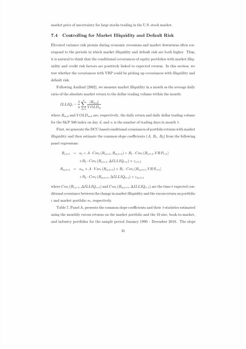
7/31/2019 Risk Uncertainty and Return
http://slidepdf.com/reader/full/risk-uncertainty-and-return 34/75
market price of uncertainty for large stocks trading in the U.S. stock market.
7.4 Controlling for Market Illiquidity and Default Risk
Elevated variance risk premia during economic recessions and market downturns often cor-
respond to the periods in which market illiquidity and default risk are both higher. Thus,
it is natural to think that the conditional covariances of equity portfolios with market illiq-
uidity and credit risk factors are positively linked to expected returns. In this section, we
test whether the covariances with VRP could be picking up covariances with illiquidity and
default risk.
Following Amihud (2002), we measure market illiquidity in a month as the average daily
ratio of the absolute market return to the dollar trading volume within the month:
ILLIQt =1
n
nd=1
|Rm,d|V OLDm
where Rm,d and V OLDm,d are, respectively, the daily return and daily dollar trading volume
for the S&P 500 index on day d, and n is the number of trading days in month t.
First, we generate the DCC-based conditional covariances of portfolio returns with market
illiquidity and then estimate the common slope coefficients (A, B1, B2) from the following
panel regressions:
Ri,t+1 = αi + A · Covt (Ri,t+1, Rm,t+1) + B1 · Covt (Ri,t+1, V R P t+1)
+B2 · Covt (Ri,t+1, ∆ILLIQt+1) + εi,t+1
Rm,t+1 = αm + A · V art (Rm,t+1) + B1 · Covt (Rm,t+1, V R P t+1)
+B2 · Covt (Rm,t+1, ∆ILLIQt+1) + εm,t+1
where Covt (Ri,t+1, ∆ILLIQt+1) and Covt (Rm,t+1, ∆ILLIQt+1) are the time-t expected con-
ditional covariance between the change in market illiquidity and the excess return on portfolio
i and market portfolio m, respectively.
Table 7, Panel A, presents the common slope coefficients and their t-statistics estimated
using the monthly excess returns on the market portfolio and the 10 size, book-to-market,
and industry portfolios for the sample period January 1990 - December 2010. The slope
31

7/31/2019 Risk Uncertainty and Return
http://slidepdf.com/reader/full/risk-uncertainty-and-return 35/75
on Covt (Ri,t+1, ∆ILLIQt+1) is found to be positive but statistically insignificant for all
equity portfolios considered in the paper. A notable point in Table 7 is that the slopes on
Covt (Ri,t+1, Rm,t+1) and Covt (Ri,t+1, V R P t+1) remain positive and highly significant after
controlling for the covariances of equity portfolios with market illiquidity.Next, we test whether the variance risk premium is proxying for default or credit risk.
We use the TED spread as an indicator of credit risk and the perceived health of the banking
system. The TED spread is the difference between the interest rates on interbank loans and
short-term U.S. government debt (T-bills). TED is an acronym formed from T-Bill and ED,
the ticker symbol for the Eurodollar futures contract.22 The size of the spread is usually
denominated in basis points (bps). For example, if the T-bill rate is 5.10% and ED trades at
5.50%, the TED spread is 40 bps. The TED spread fluctuates over time but generally has
remained within the range of 10 and 50 bps (0.1% and 0.5%) except in times of financial crisis.
A rising TED spread often presages a downturn in the U.S. stock market, as it indicates that
liquidity is being withdrawn. The TED spread is an indicator of perceived credit risk in the
general economy. This is because T-bills are considered risk-free while LIBOR reflects the
credit risk of lending to commercial banks. When the TED spread increases, that is a sign
that lenders believe the risk of default on interbank loans (also known as counterparty risk)
is increasing. Interbank lenders therefore demand a higher rate of interest, or accept lower
returns on safe investments such as T-bills. When the risk of bank defaults is considered to
be decreasing, the TED spread decreases.
We first estimate the DCC-based conditional covariances of portfolio returns with the
TED spread and then estimate the common slope coefficients from the following SUR re-
22Initially, the TED spread was the difference between the interest rates for three-month U.S. Treasuriescontracts and the three-month Eurodollars contract as represented by the London Interbank Offered Rate(LIBOR). However, since the Chicago Mercantile Exchange dropped T-bill futures, the TED spread is nowcalculated as the difference between the three-month T-bill interest rate and three-month LIBOR.
32

7/31/2019 Risk Uncertainty and Return
http://slidepdf.com/reader/full/risk-uncertainty-and-return 36/75
gressions:
Ri,t+1 = αi + A · Covt (Ri,t+1, Rm,t+1) + B1 · Covt (Ri,t+1, V R P t+1)
+B2 · Covt (Ri,t+1, ∆T EDt+1) + εi,t+1
Rm,t+1 = αm + A · V art (Rm,t+1) + B1 · Covt (Rm,t+1, V R P t+1)
+B2 · Covt (Rm,t+1, ∆T EDt+1) + εm,t+1
where Covt (Ri,t+1, ∆T EDt+1) and Covt (Rm,t+1, ∆T EDt+1) are the time-t expected condi-
tional covariance between the changes in TED spread and the excess returns on portfolio i
and market portfolio m, respectively.
Table 7, Panel A, shows the common slope coefficients and their t-statistics estimated
using the monthly excess returns on the market portfolio and the size, book-to-market, and
industry portfolios. The slope on Covt (Ri,t+1, ∆T EDt+1) is found to be positive for the size
and book-to-market portfolios, and negative for the industry portfolios. Aside from yielding
an inconsistent predictive relation with future returns, the slopes on the conditional covari-
ances with the change in TED spread are statistically insignificant for all equity portfolios.
Similar to our earlier findings, the slopes on the conditional covariances with the market
risk and uncertainty factors remain positive and highly significant after controlling for the
covariances with default risk.
Finally, we investigate the significance of risk and uncertainty coefficients after controlling
for liquidity and credit spread simultaneously:
Ri,t+1 = αi + A · Covt (Ri,t+1, Rm,t+1) + B1 · Covt (Ri,t+1, V R P t+1)
+B2 · Covt (Ri,t+1, ∆ILLIQt+1) + B3 · Covt (Ri,t+1, ∆T EDt+1) + εi,t+1
Rm,t+1 = αm + A · V art (Rm,t+1) + B1 · Covt (Rm,t+1, V R P t+1)
+B2 · Covt (Rm,t+1, ∆ILLIQt+1) + B3 · Covt (Rm,t+1, ∆T EDt+1) + εm,t+1
As shown in Panel A of Table 7, for the extended specification above, the common
slope coefficient, B2 on Covt (Ri,t+1, ∆ILLIQt+1) is estimated to be positive and marginally
significant for the book-to-market and industry portfolios, whereas B2 is insignificant for
the size portfolios. The covariances of equity portfolios with the change in TED spread do
33

7/31/2019 Risk Uncertainty and Return
http://slidepdf.com/reader/full/risk-uncertainty-and-return 37/75
not predict future returns as B3 is insignificant for all equity portfolios. Controlling for the
market illiquidity and credit risk does not affect our main findings: the market risk-return
and uncertainty-return coefficients (A and B1) are both positive and highly significant for all
equity portfolios. Equity portfolios that are highly correlated with VRP carry a significantpremium relative to portfolios that are uncorrelated or minimally correlated with VRP.
We have so far provided evidence from the individual equity portfolios (10 size, 10 book-
to-market, and 10 industry portfolios). We now investigate whether our main findings remain
intact if we use a joint estimation with all test assets simultaneously (total of 30 portfolios).
Panel B of Table 7 reports the parameter estimates and the t-statistics that are adjusted for
heteroskedasticity and autocorrelation for each series and the cross-correlations among the
error terms. As shown in the first row of Panel B, the risk aversion coefficient is estimated
to be positive and highly significant for the pooled dataset: A = 2.31 with the t-statistic
of 2.64, implying a positive and significant relation between expected return and market
risk. Similar to our earlier findings, the uncertainty aversion coefficient is also estimated to
be positive and highly significant for the joint estimation: B = 0.0053 with the t-statistic
of 3.72. These results indicate a significantly positive market price of uncertainty when all
portfolios are combined together. Equity portfolios with higher sensitivity to increases in
VRP are expected to generate higher returns next period.
The last three rows in Panel B of Table 7 provide evidence for a positive and marginally
significant relation between Covt (Ri,t+1, ∆ILLIQt+1) and future returns, indicating that the
conditional covariances of equity portfolios with the market illiquidity are positively linked to
expected returns. However, the insignificant relation between Covt (Rm,t+1, ∆T EDt+1) and
portfolio returns remains intact for the joint estimation as well. A notable point in Panel B
is that controlling for the market illiquidity and default risk individually and simultaneously
does not influence the significant predictive power of the conditional covariances of portfolio
returns with the market risk and VRP factors.
34

7/31/2019 Risk Uncertainty and Return
http://slidepdf.com/reader/full/risk-uncertainty-and-return 38/75
8 Cross-Sectional Relation between VRP-beta and Ex-pected Returns
In this section, we investigate the cross-sectional asset pricing performance of our model
by testing the significance of a cross-sectional relation between expected returns on equity
portfolios and the portfolios’ conditional covariances with VRP. Following Bali (2008) and
Campbell, Giglio, Polk, and Turley (2012), we use the 25 and 100 Size and Book-to-Market
(BM) portfolios of Kenneth French as test assets.23 First, we estimate the DCC-based
conditional covariances of 25 and 100 Size/BM portfolios with VRP and then for each month
we form quintile portfolios sorted based on the portfolios’ conditional covariances (or betas)
with VRP. Since the conditional variance of VRP is the same across portfolios, we basically
sort equity portfolios based on their VRP-beta:
V RP betai,t =
cov[Ri,t+1, V R P t+1|Ωt]
var [V RP t+1|Ωt], (33)
where V RP betai,t is the VRP-beta of portfolio i in month t, cov[Ri,t+1, V R P t+1|Ωt] is the condi-
tional covariance of portfolio i with VRP estimated using equation (26), and var [V RP t+1|Ωt]
is the conditional variance of VRP which is constant in the cross-section of equity portfolios.
Table 8 presents the average excess monthly returns of quintile portfolios that are formed
by sorting the 25 and 100 Size/BM portfolios based on their VRP-beta. When we use the 25
Size/BM portfolios as test assets, each quintile arbitrage portfolio has a total of five Size/BM
portfolios. Similarly, when we use the 100 Size/BM portfolios as test assets, each arbitrage
portfolio has a total of 20 Size/BM portfolios. The results are presented for the sample
period January 1990 to December 2010.
In Table 8, Q1 (Low V RP beta) is the quintile portfolio of Size/BM portfolios with the
lowest VRP-beta during the past month, and Q5 (High V RP beta) is the quintile portfolio of
Size/BM portfolios with the highest VRP-beta during the previous month. As shown in the
left panel of Table 8, when the 25 Size/BM portfolios are used, the average excess return
increases from 0.38% per month to 0.96% per month as we move from Q1 to Q5, generating
2325 Size/BM and 100 Size/BM portfolios are described in and obtained from Kenneth French’s datalibrary.
35
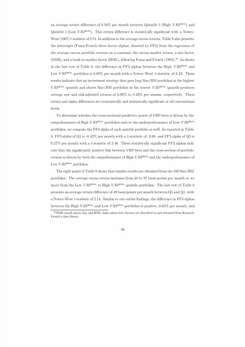
7/31/2019 Risk Uncertainty and Return
http://slidepdf.com/reader/full/risk-uncertainty-and-return 39/75
an average return difference of 0.58% per month between Quintile 5 (High V RP beta) and
Quintile 1 (Low V RP beta). This return difference is statistically significant with a Newey-
West (1987) t-statistic of 2.51. In addition to the average excess returns, Table 8 also presents
the intercepts (Fama-French three-factor alphas, denoted by FF3) from the regression of the average excess portfolio returns on a constant, the excess market return, a size factor
(SMB), and a book-to-market factor (HML), following Fama and French (1993).24 As shown
in the last row of Table 8, the difference in FF3 alphas between the High V RP beta and
Low V RP beta portfolios is 0.69% per month with a Newey-West t-statistic of 3.33. These
results indicate that an investment strategy that goes long Size/BM portfolios in the highest
V RP beta quintile and shorts Size/BM portfolios in the lowest V RP beta quintile produces
average raw and risk-adjusted returns of 6.96% to 8.28% per annum, respectively. These
return and alpha differences are economically and statistically significant at all conventional
levels.
To determine whether the cross-sectional predictive power of VRP-beta is driven by the
outperformance of High V RP beta portfolios and/or the underperformance of Low V RP beta
portfolios, we compute the FF3 alpha of each quintile portfolio as well. As reported in Table
8, FF3 alpha of Q1 is -0.42% per month with a t-statistic of -2.66, and FF3 alpha of Q5 is
0.27% per month with a t-statistic of 2.46. These statistically significant FF3 alphas indi-
cate that the significantly positive link between VRP-beta and the cross-section of portfolio
returns is driven by both the outperformance of High V RP beta and the underperformance of
Low V RP beta portfolios.
The right panel of Table 8 shows that similar results are obtained from the 100 Size/BM
portfolios. The average excess return increases from 48 to 97 basis points per month as we
move from the Low V RP beta to High V RP beta quintile portfolios. The last row of Table 8
presents an average return difference of 49 basis points per month between Q5 and Q1, with
a Newey-West t-statistic of 2.14. Similar to our earlier findings, the difference in FF3 alphas
between the High V RP beta and Low V RP beta portfolios is positive, 0.65% per month, and
24SMB (small minus big) and HML (high minus low) factors are described in and obtained from KennethFrench’s data library.
36

7/31/2019 Risk Uncertainty and Return
http://slidepdf.com/reader/full/risk-uncertainty-and-return 40/75
highly significant with a t-statistic of 2.70. These results indicate that the equity portfolios
in highest V RP beta quintile generate 5.88% to 7.80% more annual raw and risk-adjusted
returns compared to the equity portfolios in the lowest V RP beta quintile. As shown in the
last column of Table 8, FF3 alpha of Q1 is -0.37% per month with a t-statistic of -2.61, andFF3 alpha of Q5 is 0.28% per month with a t-statistic of 2.10, implying that the significantly
positive link between VRP-beta and the cross-section of expected returns on the 100 Size/BM
portfolios is driven by both the outperformance of High V RP beta and the underperformance
of Low V RP beta portfolios.
We now examine the cross-sectional relation between VRP-beta, Market-beta and ex-
pected returns using Fama and MacBeth (1973) regressions. We calculate the time-series
averages of the slope coefficients from the regressions of one-month ahead portfolio returns on
the conditional covariances of portfolios with the market and VRP factors, Covt (Ri,t+1, Rm,t+1)
and Covt (Ri,t+1, V R P t+1). The average slopes provide standard Fama-MacBeth tests for
determining whether the market and/or uncertainty factors on average have non-zero premi-
ums. Monthly cross-sectional regressions are run for the following asset pricing specification:
Ri,t+1 = λ0,t + λ1,t · Covt (Ri,t+1, Rm,t+1) + λ2,t · Covt (Ri,t+1, V R P t+1) + εi,t+1
where Ri,t+1 is the excess return on portfolio i in month t + 1, λ1,t and λ2,t are the monthly
slope coefficients on Covt (Ri,t+1, Rm,t+1) and Covt (Ri,t+1, V R P t+1), respectively. The pre-
dictive cross-sectional regressions of Ri,t+1 are run on the time-t expected conditional covari-
ances of portfolios with the market and VRP factors.
We compute the time series averages of the slope coefficients (λ1, λ2) over the 252 months
from January 1990 to December 2010 for both the 25 and 100 Size/BM portfolios. The
bivariate regression results produce a positive and statistically significant relation between
Covt (Ri,t+1, V R P t+1) and the cross-section of portfolios returns. The average slope, λ2, is
estimated to be 0.0603 with a Newey-West t-statistic of 2.25 for the 25 Size/BM portfolios,
and 0.0176 with a Newey-West t-statistic of 2.15 for the 100 Size/BM portfolios. Although
we find a robust, significantly positive link between VRP-beta and expected returns from the
Fama-MacBeth regressions, the cross-sectional relation between market beta and expected
37
7/31/2019 Risk Uncertainty and Return
http://slidepdf.com/reader/full/risk-uncertainty-and-return 41/75
returns turns out to be sensitive to the choice of test assets. Specifically, the average slope,
λ1, is found to be 7.78 with a t-statistic of 1.94 for the 25 Size/BM portfolios, whereas it is
positive, but statistically insignificant for the 100 Size/BM portfolios.
The economic significance of the monthly slope coefficients from the Fama-MacBethregressions can be interpreted based on the long-short equity portfolios. First, we com-
pute the average values of Covt (Ri,t+1, V R P t+1) for the Size/BM portfolios sorted into the
quintile portfolios. For the 25 Size/BM portfolios, the average Covt (Ri,t+1, V R P t+1) val-
ues are −1.0150 for Quintile 1, −0.8049 for Quintile 2, −0.7104 for Quintile 3, −0.6478
for Quintile 4, and −0.5655 for Quintile 5.25 Hence, the difference in Covt (Ri,t+1, V R P t+1)
values between equity portfolios in the Low V RP beta and High V RP beta quintiles is 0.4495
(= −0.5655 − (−1.0150)). To be consistent with our univariate portfolio results in Ta-
ble 8, we run a univariate regression of Ri,t+1 on Covt (Ri,t+1, V R P t+1), and the average
slope of 0.0149 implies that the equity portfolios in highest V RP beta quintile generate 0.67%
(0.0149 × 0.4495 = 0.67%) more monthly returns compared to the equity portfolios in the
lowest V RP beta quintile.
To determine the economic significance of the slope coefficients for the 100 Size/BM port-
folios, we calculate the average Covt (Ri,t+1, V R P t+1) values for each quintile portfolio as well:
−1.0872 for Quintile 1, −0.8206 for Quintile 2, −0.7150 for Quintile 3, −0.6308 for Quintile
4, and −0.5053 for Quintile 5. Hence, the difference in Covt (Ri,t+1, V R P t+1) values between
equity portfolios in the Low V RP beta and High V RP beta quintiles is 0.5819. The univariate
Fama-MacBeth regressions of one-month ahead portfolio returns on Covt (Ri,t+1, V R P t+1)
yields an average slope coefficient of 0.0103 for the 100 Size/BM portfolios. This positive
and significant average slope coefficient implies that buying the Size/BM portfolios in high-
est V RP beta quintile and short-selling the Size/BM portfolios in the lowest V RP beta quintile
generate a 0.60% return in the following month. These return magnitudes implied by the
Fama-MacBeth slope coefficients (0.67% and 0.60% per month) are in line with the univariate
portfolio results reported in Table 8 (0.58% and 0.49% per month, respectively).
25The negative values for the conditional covariances of equity portfolios with the VRP factor are consistentwith the negative value for conditional covariance of the market return with the VRP factor reported earlierin Section 6.2.
38

7/31/2019 Risk Uncertainty and Return
http://slidepdf.com/reader/full/risk-uncertainty-and-return 42/75
9 Conclusion
Although uncertainty is more common in decision-making process than risk, relatively little
attention is paid to the phenomenon of uncertainty in empirical asset pricing literature. This
paper focuses on economic uncertainty and augments the original consumption-based CAPM
to incorporate the time-varying volatility of the consumption growth and the volatility un-
certainty in the consumption growth process. According to the augmented asset pricing
model, the premium on equity is composed of two separate terms; the first term compensat-
ing for the standard consumption risk and the second term representing a true premium for
variance risk. We find that in the presence of volatility uncertainty, both market risk and
volatility uncertainty carry a positive premium, which is consistent with an economy where
the intertemporal elasticity of substitution (IES) is larger than one.
Since information about consumption volatility uncertainty is too imprecise to measure
with available data, we have to come up with a proxy for volatility uncertainty that should be
consistent with our underlying economic model. Following Zhou (2010), we measure volatility
uncertainty with the variance risk premium (VRP) of the aggregate stock market portfolio.
Different from earlier studies, we provide empirical evidence that VRP is indeed closely
related to economic and financial market uncertainty. Specifically, we generate several proxiesfor uncertainty based on the macroeconomic variables, return distributions of financial firms,
credit default swap market, and investors’ disagreement about individual stocks. We show
that VRP is highly correlated with all measures of uncertainty.
Based on the two-factor asset pricing model, we investigate whether the market prices of
risk and uncertainty are economically and statistically significant in the U.S. equity market.
Using the dynamic conditional correlation (DCC) model of Engle (2002), we estimate equity
portfolios’ conditional covariances with the market portfolio and VRP factors and then test
whether these dynamic conditional covariances predict future returns on equity portfolios.
The empirical results from the size, book-to-market, and industry portfolios indicate that
the DCC-based conditional covariances of equity portfolios with the market and VRP factors
predict the time-series and cross-sectional variation in stock returns. We find the risk-return
39

7/31/2019 Risk Uncertainty and Return
http://slidepdf.com/reader/full/risk-uncertainty-and-return 43/75
coefficients to be positive and highly significant, implying a strongly positive link between
expected return and market risk. Similarly, the results indicate a significantly positive market
price of uncertainty. That is, equity portfolios that are highly correlated with uncertainty
(proxied by VRP) carry a significant premium relative to portfolios that are uncorrelatedor minimally correlated with VRP. In addition to the size, book-to-market, and industry
portfolios, we investigate the significance of risk, uncertainty, and return tradeoffs using the
largest 500 stocks trading at NYSE, AMEX, and NASDAQ as well as stocks in the S&P
500 index. Consistent with our findings from equity portfolios, we find significantly positive
market prices of risk and uncertainty for large stocks trading in the U.S. equity market.
We also examine whether the conditional covariances with VRP could be picking up
the covariances with market illiquidity and/or default risk. We find that the significantly
positive link between market covariance risk, uncertainty and future returns remain intact
after controlling for liquidity and credit risk.
Finally, we investigate the cross-sectional asset pricing performance of our model using
the long-short equity portfolios and the Fama-MacBeth regressions. The results indicate that
the annual average raw and risk-adjusted returns of the equity portfolios in the highest VRP-
beta quintile are 6 to 8 percent higher than the annual average returns of the equity portfolios
in the lowest VRP-beta quintile. After controlling for the market, size, and book-to-market
factors of Fama and French (1993), the positive relation between VRP-beta and the cross-
section of portfolio returns remains economically and statistically significant. Overall, we
conclude that the time-varying exposures of equity portfolios to the variance risk premia
predict the time-series and cross-sectional variation in stock returns.
40

7/31/2019 Risk Uncertainty and Return
http://slidepdf.com/reader/full/risk-uncertainty-and-return 44/75
References
Amihud, Yakov (2002), “Illiquidity and Stock Returns: Cross-Section and Time-Series Ef-
fects,” Journal of Financial Markets, vol. 5, 31–56.
Andersen, Torben G., Tim Bollerslev, Francis X. Diebold, and Heiko Ebens (2001), “TheDistribution of Realized Stock Return Volatility,” Journal of Financial Economics , vol. 61,
43–76.
Andersen, Torben G., Tim Bollerslev, Francis X. Diebold, and Paul Labys (2003), “Modeling
and Forecasting Realized Volatility,” Econometrica , vol. 71, 579–625.
Anderson, Evan W., Eric Ghysels, and Jennifer L. Juergens (2009), “The Impact of Risk and
Uncertainty on Expected Returns,” Journal of Financial Economics , vol. 94, 233–263.
Bakshi, Gurdip and Dilip Madan (2000), “Spanning and Derivative-Security Valuation,”Journal of Financial Economics , vol. 55, 205–238.
Bakshi, Gurdip and Dilip Madan (2006), “A Theory of Volatility Spread,” Management
Science, vol. 52, 1945–1956.
Bali, Turan G. (2008), “The Intertemporal Relation between Expected Returns and Risk,”
Journal of Financial Economics , vol. 87, 101–131.
Bali, Turan G. and Robert F. Engle (2010), “The Intertemporal Capital Asset Pricing Model
with Dynamic Conditional Correlations,” Journal of Monetary Economics , vol. 57, 377–
390.
Bansal, Ravi, Dana Kiku, and Amir Yaron (2007), “A Note on the Economics and Statistics
of Predictability: A Long Run Risks Perspective,” Working Paper, Duke University and
University of Pennsylvania.
Bansal, Ravi, Dana Kiku, and Amir Yaron (2009), “An Empirical Evaluation of the Long-
Run Risks Model for Asset Prices,” Duke University and University of Pennsylvania.
Bansal, Ravi and Amir Yaron (2004), “Risks for the Long Run: A Potential Resolution of
Asset Pricing Puzzles,” Journal of Finance, vol. 59, 1481–1509.
Barndorff-Nielsen, Ole and Neil Shephard (2002), “Econometric Analysis of Realised Volatil-
ity and Its Use in Estimating Stochastic Volatility Models,” Journal of Royal Statistical
Society, Series B , vol. 64, 253–280.
Beeler, Jason and John Y. Campbell (2009), “The Long-Run Risks Model and Aggregate
Asset Prices: An Empirical Assessment,” Working Paper, Harvard University.
41

7/31/2019 Risk Uncertainty and Return
http://slidepdf.com/reader/full/risk-uncertainty-and-return 45/75
Bekaert, Geert, Eric Engstrom, and Yuhang Xing (2009), “Risk, Uncertainty, and Asset
Prices,” Journal of Financial Economics , vol. 91, 59–82.
Bollerslev, Tim (1986), “Generalized Autoregressive Conditional Heteroskedasticity,” Jour-
nal of Econometrics, vol. 31, 307–327.
Bollerslev, Tim, Robert F. Engle, and Jeffrey M. Wooldridge (1988), “A Capital Asset
Pricing Model with Time Varying Covariances,” Journal of Political Economy , vol. 96,
116–131.
Bollerslev, Tim, Mike Gibson, and Hao Zhou (2011a), “Dynamic Estimation of Volatility
Risk Premia and Investor Risk Aversion from Option-Implied and Realized Volatilities,”
Journal of Econometrics , vol. 160, 102–118.
Bollerslev, Tim, James Marrone, Lai Xu, and Hao Zhou (2011b), “Stock Return Predictabil-
ity and Variance Risk Premia: Statistical Inference and International Evidence,” WorkingPaper.
Bollerslev, Tim, George Tauchen, and Hao Zhou (2009), “Expected Stock Returns and
Variance Risk Premia,” Review of Financial Studies, vol. 22, 4463–4492.
Bollerslev, Tim and Hao Zhou (2007), “Expected Stock Returns and Variance Risk Premia,”
Finance and Economics Disucussion Series 2007-11 , Federal Reserve Board.
Breeden, Douglas and Robert Litzenberger (1978), “Prices of State-Contingent Claims Im-
plicit in Option Prices,” Journal of Business , vol. 51, 621–651.
Britten-Jones, Mark and Anthony Neuberger (2000), “Option Prices, Implied Price Pro-
cesses, and Stochastic Volatility,” Journal of Finance, vol. 55, 839–866.
Buraschi, Andrea, Fabio Trojani, and Andrea Vedolin (2009), “The Joint Behavior of Credit
Spreads, Stock Options and Equity Returns When Investors Disagree,” Imperial College
London Working Paper.
Campbell, John Y. (1987), “Stock Returns and the Term Structure,” Journal of Financial
Economics , vol. 18, 373–399.
Campbell, John Y. (1993), “Intertemporal Asset Pricing without Consumption Data,” Amer-
ican Economic Review , vol. 83, 487–515.
Campbell, John Y. (1996), “Understanding Risk and Return,” Joumal of Political Economy ,
vol. 104, 298–345.
42

7/31/2019 Risk Uncertainty and Return
http://slidepdf.com/reader/full/risk-uncertainty-and-return 46/75
Campbell, John Y. (1999), Handbook of Macroeconomics, vol. 1, chap. Asset Prices, Con-
sumption, and the Business Cycle, pages 1231–1303.
Campbell, John Y., Stefano Giglio, Christopher Polk, and Robert Turley (2012), “An In-
tertemporal CAPM with Stochastic Volatility,” Working Paper, Harvard University.
Campbell, John Y. and Robert J. Shiller (1988), “The Dividend-Price Ratio and Expec-
tations of Future Dividends and Discount Factors,” Review of Financial Studies, vol. 1,
195–228.
Campbell, Sean D. and Francis X. Diebold (2009), “Stock Returns and Expected Busi-
ness Conditions: Half a Century of Direct Evidence,” Journal of Business and Economic
Statistics, vol. 27, 266–278.
Carr, Peter and Dilip Madan (1998), “Towards a Theory of Volatility Trading,” in Volatil-
ity: New Estimation Techniques for Pricing Derivatives , chap.29, 417-427, Robert Jarrow(ed.). London: Risk Books.
Carr, Peter and Liuren Wu (2009), “Variance Risk Premiums,” Review of Financial Studies ,
vol. 22, 1311–1341.
Chen, Xiaohong, Jack Favilukis, and Sydney C. Ludvigson (2011), “An Estimation of Eco-
nomic Models with Recursive Preferences,” Working Paper, Yale University and New York
University.
Chen, Zengjing and Larry G. Epstein (2002), “Ambiguity, Risk, and Asset Returns in Con-tinuous Time,” Econometrica , vol. 4, 1403–1445.
Diether, Karl, Christopher Malloy, and Anna Scherbina (2002), “Differences of Opinion and
the Cross-Section of Stock Returns,” Journal of Finance, vol. 57, 2113–2141.
Drechsler, Itamar and Amir Yaron (2011), “What’s Vol Got to Do With It,” Review of
Financial Studies, vol. 24, 1–45.
Ellsberg, Daniel (1961), “Risk, Ambiguity, and the Savage Axiom,” Quarterly Journal of
Economics , vol. 75, 643–669.
Engle, Robert F. (2002), “Dynamic Conditional Correlation: A Simple Class of Multivariate
Generalized Autoregressive Conditional Heteroskedasticity Models,” Journal of Business
and Economic statistics , vol. 20, 339–350.
Epstein, Larry G. (1999), “A Definition of Uncertainty Aversion,” Review of Economic
Studies, vol. 66, 679–708.
43

7/31/2019 Risk Uncertainty and Return
http://slidepdf.com/reader/full/risk-uncertainty-and-return 47/75
Epstein, Larry G. and Tan Wang (1994), “Intertemporal Asset Pricing under Knightian
Uncertainty,” Econometrica , vol. 62, 283–322.
Epstein, Larry G. and Jiankang Zhang (2001), “Subjective Probabilities on Subjectively
Unambiguous Events,” Econometrica , vol. 69, 265–306.
Fama, Eugene F. and Kenneth R. French (1988), “Dividend Yields and Expected Stock
Returns,” Journal of Financial Economics , vol. 22, 3–25.
Fama, Eugene F. and Kenneth R. French (1989), “Business Conditions and Expected Returns
on Stocks and Bonds,” Journal of Financial Economics , vol. 25, 23–49.
Fama, Eugene F. and Kenneth R. French (1992), “The Cross-Section of Expected Stock
Returns,” Journal of Finance, vol. 47, 427–465.
Fama, Eugene F. and Kenneth R. French (1993), “Common Risk Factors in the Returns onStocks and Bonds,” Journal of Financial Economics , vol. 33, 3–56.
Fama, Eugene F. and James MacBeth (1973), “Risk, Return, and Equilibrium: Empirical
Tests,” Journal of Political Economy , vol. 71, 607–636.
Ferson, Wayne E. and Campbell R. Harvey (1991), “The Variation in Economic Risk Pre-
miums,” Journal of Political Economy , vol. 99, 385–415.
Gabaix, Xavier (2011), “Variable Rare Disasters: An Exactly Solved Framework for Ten
Puzzles in Macro-Finance,” Quarterly Journal of Economics, forthcoming.
Ghysels, Eric, Pedro Santa-Clara, and Ross Valkanov (2005), “There is a Risk-Return Trade-
off After All,” Journal of Financial Economics , vol. 76, 509–548.
Glosten, Lawrence R., Ravi Jagannathan, and David E. Runkle (1993), “On the Relation
between the Expected Value and the Volatility of the Nominal Excess Returns on Stocks,”
Journal of Finance, vol. 48, 1779–1801.
Goetzmann, William N., Akiko Watanabe, and Masahiro Watanabe (2009), “Investor Expec-
tations, Business Conditions, and the Pricing of Beta-Instability Risk,” Yale ICF Working
Paper.
Guo, Hui and Robert Savickas (2006), “Idiosyncratic Volatility, Stock Market Volatility, and
Expected Stock Returns,” Journal of Business and Economic Statistics , vol. 24, 43–56.
Guo, Hui and Robert F. Whitelaw (2006), “Uncovering the Risk-Return Relation in the
Stock Market,” Journal of Finance, vol. 61, 1433–1463.
44

7/31/2019 Risk Uncertainty and Return
http://slidepdf.com/reader/full/risk-uncertainty-and-return 48/75
Hall, Robert (1988), “Intertemporal Substitution in Consumption,” Journal of Political
Economy , vol. 96, 339–357.
Jiang, George and Yisong Tian (2005), “Model-Free Implied Volatility and Its Information
Content,” Review of Financial Studies, vol. 18, 1305–1342.
Ju, Nengjiu and Jianjun Miao (2012), “Ambiguity, Learning, and Asset Returns,” Econo-
metrica , forthcoming.
Kandel, Shmuel and Robert F. Stambaugh (1991), “Asset Returns and Intertemporal Pref-
erences,” Journal of Monetary Economics, vol. 27, 39–71.
Kelly, Bryan T. (2011), “Tail Risk and Asset Prices,” Chicago-Booth School of Business
Working Paper.
Klibanoff, Peter, Massimo Marinacci, and Sujoy Mukerji (2005), “A Smooth Model of Deci-sion Making under Ambiguity,” Econometrica , vol. 73, 1849–1892.
Knight, Frank H. (1921), Risk, Uncertainty and Profit , Houghton Mifflin Co., Boston, MA.
Lintner, John (1965), “The Valuation of Risky Assets and the Selection of Risky Investments
in the Portfolios and Capital Budgets,” Review of Economics and Statistics , vol. 47, 13–37.
Liu, Ming, Harold H. Zhang, and Xinting Fan (2011), “Momentum and Contrarian Profits
and Macroeconomic Fundamentals,” Working Paper, University of Texas at Dallas.
Londono, Juan-Miguel (2010), “The Variance Risk Premium around the World,” WorkingPaper, Tilburg University Department of Finance, The Netherlands.
Lundblad, Christian (2007), “The Risk Return Tradeoff in the Long Run: 1836-2003,” Jour-
nal of Financial Economics , vol. 85, 123–150.
Maccheroni, Fabio, Massimo Marinacci, and Aldo Rustichini (2006), “Ambiguity Aversion,
Robustness, and the Variational Representation of Preferences,” Econometrica , vol. 74,
1447–1498.
Martin, Ian (2011), “Simple Variance Swaps,” NBER Working Paper 16884.
Merton, Robert C. (1973), “An Intertemporal Capital Asset Pricing Model,” Econometrica ,
vol. 41, 867–887.
Merton, Robert C. (1980), “On Estimating the Expected Return on the Market,” Journal
of Financial Economics , vol. 8, 323–361.
45
7/31/2019 Risk Uncertainty and Return
http://slidepdf.com/reader/full/risk-uncertainty-and-return 49/75
Mueller, Philippe, Andrea Vedolin, and Hao Zhou (2011), “Short-Run Bond Risk Premia,”
Working Paper, Federal Reserve Board.
Newey, Whitney K. and Kenneth D. West (1987), “A Simple Positive Semi-Definite,
Heteroskedasticity and Autocorrelation Consistent Covariance Matrix,” Econometrica ,
vol. 55, 703–708.
Rosenberg, Joshua V. and Robert F. Engle (2002), “Empirical Pricing Kernels,” Journal of
Financial Economics, vol. 64, 341–372.
Schmeidler, David (1989), “Subjective Probability and Expected Utility without Additivity,”
Econometrica , vol. 57, 571–587.
Sharpe, William (1964), “Capital Asset Prices: A Theory of Market Equilibrium under
Conditions of Risk,” Journal of Finance, vol. 19, 425–442.
Shumway, Tyler (1997), “The Delisting Bias in CRSP Data,” Journal of Finance, vol. 52,
327–340.
Wang, Hao, Hao Zhou, and Yi Zhou (2011), “Credit Default Swap Spreads and Variance
Risk Premia,” Working Paper, Federal Reserve Board.
Zhou, Hao (2010), “Variance Risk Premia, Asset Predictability Puzzles, and Macroeconomic
Uncertainty,” Working Paper, Federal Reserve Board.
46

7/31/2019 Risk Uncertainty and Return
http://slidepdf.com/reader/full/risk-uncertainty-and-return 50/75
Table 1 Model Calibration Parameter Setting
This table reports the calibration parameter values for the stochastic volatility-of-volatility model used in thispaper. BTZ2009 refers to the calibration setting of Bollerslev, Tauchen, and Zhou (2009), with an emphasison equity risk premium and its short-run predictability, while the setting of Zhou (2010) also considers bond
risk premium and credit spread and their forecastability from variance risk premium. The Campbell-Shillerlinearization constants are κ1 = 0.9 and κ0 = 0.3251.
Calibration Parameters BTZ2009 Zhou (2010)
Preference Parameters: δ = 0.997 δ = 0.997
γ = 10 γ = 2
ψ = 1.5 ψ = 1.5
Endowment Parameters: µg = 0.0015 µg = 0.0015
aσ = 1.34 × 10⁻⁶ aσ = 0.002
ρσ = 0.978 ρσ = 0.1aq = 2 × 10⁻⁷ aq = 1.4 × 10⁻⁵
ρq = 0.8 ρq = 0.98
ϕq = 0.001 ϕq = 0.008
Risk-Return Trade-off (A) 10 2
Uncertainty-Return Trade-off (B) 10.24 0.08
47

7/31/2019 Risk Uncertainty and Return
http://slidepdf.com/reader/full/risk-uncertainty-and-return 51/75
Table 2 Results from Ten Decile Size, Book-to-Market, and Industry Portfolios
This table reports the portfolio-specific intercepts and the common slope estimates from the following panel regression:
Ri,t+1 = αi + A · Covt (Ri,t+1, Rm,t+1) + B · Covt (Ri,t+1, V RP t+1) + εi,t+1
Rm,t+1 = αm + A · V art (Rm,t+1) + B · Covt (Rm,t+1, V RP t+1) + εm,t+1
where Covt (Ri,t+1, Rm,t+1) is the time-t expected conditional covariance between the excess return on portfolio i (Ri,t+1)and the excess return on the market portfolio (Rm,t+1 ), Covt (Ri,t+1, V RP t+1) is the time-t expected conditional covariancebetween the excess return on portfolio i and the variance risk premia (V RP t+1), Covt (Rm,t+1, V RP t+1) is the time-t expectedconditional covariance between the excess return on the market portfolio m and the variance risk premia (V RP t+1), andV art (Rm,t+1) is the time-t expected conditional variance of excess returns on the market portfolio. The parameters and theirt-statistics are estimated using the monthly excess returns on the market portfolio and the ten decile size, book-to-market, andindustry portfolios for the sample period from January 1990 to December 2010. The alphas (αi) are reported for each equityportfolio and the t-statistics are presented in parentheses. The t-statistics are adjusted for heteroskedasticity and autocorrelationfor each series and cross-correlations among the portfolios. The last four rows, respectively, show the common slope coefficients(A and B), the Wald1 statistics from testing the joint hypothesis H 0 : α1 = α2 = ...αm = 0 , and the Wald2 statistics fromtesting the equality of Alphas for high-return and low-return portfolios (Small vs. Big; Value vs. Growth; and HiTec vs. Telcm).The p-values of Wald1 and Wald2 statistics are given in square brackets.
Size αi, αm BM αi, αm Industry αi, αm
Small 0.0041 Growth 0.0036 NoDur 0.0043
(0.94) (0.90) (1.53)
2 0.0022 2 0.0048 Durbl 0.0019
(0.48) (1.38) (0.37)
3 0.0025 3 0.0053 Manuf 0.0046
(0.58) (1.58) (1.26)
4 0.0015 4 0.0065 Enrgy 0.0059
(0.35) (1.88) (1.88)
5 0.0023 5 0.0057 HiTec 0.0026
(0.54) (1.74) (0.45)
6 0.0023 6 0.0051 Telcm -0.0005
(0.61) (1.51) (-0.13)
7 0.0028 7 0.0058 Shops 0.0028
(0.76) (1.78) (0.80)
8 0.0020 8 0.0059 Hlth 0.0036
(0.53) (1.76) (1.13)
9 0.0023 9 0.0067 Utils 0.0038
(0.67) (1.94) (1.39)
Big 0.0001 Value 0.0082 Other 0.0018
(0.01) (1.90) (0.47)
Market 0.0008 Market 0.0032 Market 0.0019
(0.17) (1.23) (0.55)
A 3.9562 A 2.5101 A 3.4055
(3.12) (2.53) (2.35)
B 0.0058 B 0.0050 B 0.0060
(2.97) (2.27) (2.78)
Wald1 16.74 Wald1 8.88 Wald1 14.35
[0.12] [0.63] [0.21]
Wald2 1.56 Wald2 1.79 Wald2 0.40
[0.21] [0.18] [0.53]
48
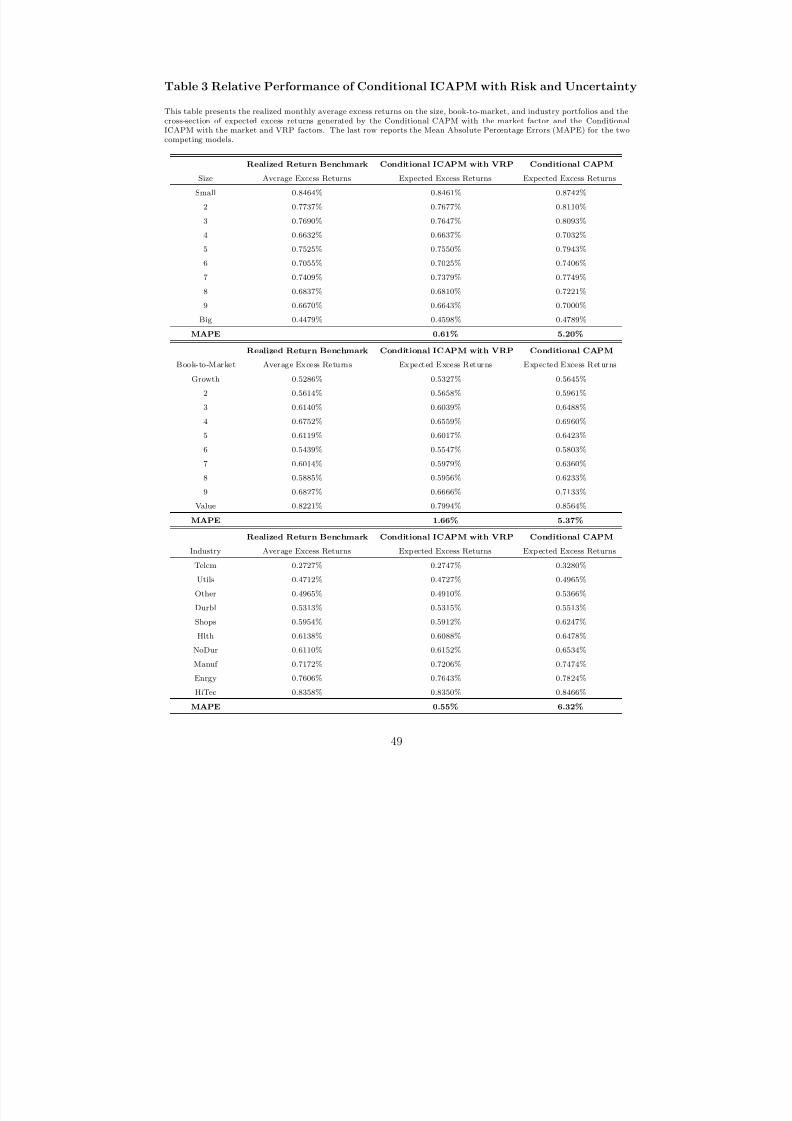
7/31/2019 Risk Uncertainty and Return
http://slidepdf.com/reader/full/risk-uncertainty-and-return 52/75
Table 3 Relative Performance of Conditional ICAPM with Risk and Uncertainty
This table presents the realized monthly average excess returns on the size, book-to-market, and industry portfolios and thecross-section of expected excess returns generated by the Conditional CAPM with the market factor and the ConditionalICAPM with the market and VRP factors. The last row reports the Mean Absolute Percentage Errors (MAPE) for the twocompeting models.
Realized Return Benchmark Conditional ICAPM with VRP Conditional CAPM
Size Average Excess Returns Expected Excess Returns Expected Excess Returns
Small 0.8464% 0.8461% 0.8742%
2 0.7737% 0.7677% 0.8110%
3 0.7690% 0.7647% 0.8093%
4 0.6632% 0.6637% 0.7032%
5 0.7525% 0.7550% 0.7943%
6 0.7055% 0.7025% 0.7406%
7 0.7409% 0.7379% 0.7749%
8 0.6837% 0.6810% 0.7221%
9 0.6670% 0.6643% 0.7000%
Big 0.4479% 0.4598% 0.4789%
MAPE 0.61% 5.20%
Realized Return Benchmark Conditional ICAPM with VRP Conditional CAPM
Book-to-Market Average Excess Returns Expected Excess Returns Expected Excess Returns
Growth 0.5286% 0.5327% 0.5645%
2 0.5614% 0.5658% 0.5961%
3 0.6140% 0.6039% 0.6488%
4 0.6752% 0.6559% 0.6960%
5 0.6119% 0.6017% 0.6423%
6 0.5439% 0.5547% 0.5803%
7 0.6014% 0.5979% 0.6360%
8 0.5885% 0.5956% 0.6233%
9 0.6827% 0.6666% 0.7133%
Value 0.8221% 0.7994% 0.8564%
MAPE 1.66% 5.37%
Realized Return Benchmark Conditional ICAPM with VRP Conditional CAPM
Industry Average Excess Returns Exp ected Excess Returns Exp ected Excess Returns
Telcm 0.2727% 0.2747% 0.3280%
Utils 0.4712% 0.4727% 0.4965%
Other 0.4965% 0.4910% 0.5366%
Durbl 0.5313% 0.5315% 0.5513%
Shops 0.5954% 0.5912% 0.6247%
Hlth 0.6138% 0.6088% 0.6478%
NoDur 0.6110% 0.6152% 0.6534%
Manuf 0.7172% 0.7206% 0.7474%
Enrgy 0.7606% 0.7643% 0.7824%
HiTec 0.8358% 0.8350% 0.8466%
MAPE 0.55% 6.32%
49
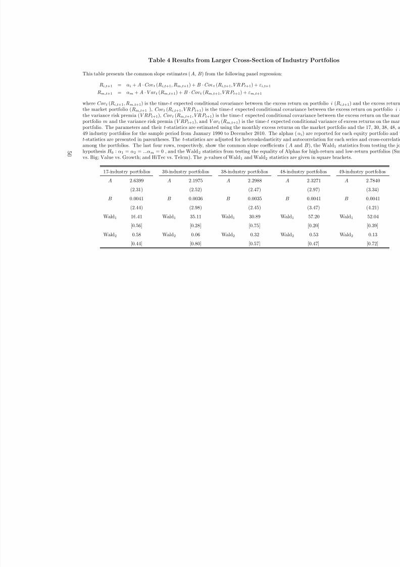
7/31/2019 Risk Uncertainty and Return
http://slidepdf.com/reader/full/risk-uncertainty-and-return 53/75
Table 4 Results from Larger Cross-Section of Industry Portfolio
This table presents the common slope estimates (A, B) from the following panel regression:Ri,t+1 = αi + A · Covt (Ri,t+1, Rm,t+1) + B · Covt (Ri,t+1, V R P t+1) + εi,t+1
Rm,t+1 = αm + A · V art (Rm,t+1) + B · Covt (Rm,t+1, V R P t+1) + εm,t+1
where Covt (Ri,t+1, Rm,t+1) is the time-t expected conditional covariance between the excess return on portfolio i
the market portfolio (Rm,t+1 ), Covt (Ri,t+1, V R P t+1) is the time-t expected conditional covariance between thethe variance risk premia (V RP t+1), Covt (Rm,t+1, V R P t+1) is the time-t expected conditional covariance betweenportfolio m and the variance risk premia (V RP t+1), and V art (Rm,t+1) is the time-t expected conditional variancportfolio. The parameters and their t-statistics are estimated using the monthly excess returns on the market por49 industry portfolios for the sample period from January 1990 to December 2010. The alphas (αi) are reported t-statistics are presented in parentheses. The t-statistics are adjusted for heteroskedasticity and autocorrelation for among the portfolios. The last four rows, respectively, show the common slope coefficients (A and B), the Wald
hypothesis H 0 : α1 = α2 = ...αm = 0 , and the Wald2 statistics from testing the equality of Alphas for high-returnvs. Big; Value vs. Growth; and HiTec vs. Telcm). The p-values of Wald1 and Wald2 statistics are given in square b
17-industry portfolios 30-industry portfolios 38-industry portfolios 48-industry portfolios
A 2.6399 A 2.1975 A 2.2988 A 2.3271
(2.31) (2.52) (2.47) (2.97)
B 0.0041 B 0.0036 B 0.0035 B 0.0041
(2.44) (2.98) (2.45) (3.47)
Wald1 16.41 Wald1 35.11 Wald1 30.89 Wald1 57.20
[0.56] [0.28] [0.75] [0.20]
Wald2 0.58 Wald2 0.06 Wald2 0.32 Wald2 0.53
[0.44] [0.80] [0.57] [0.47]
5 0

7/31/2019 Risk Uncertainty and Return
http://slidepdf.com/reader/full/risk-uncertainty-and-return 54/75
Table 5 Controlling for Macroeconomic Variables
This table presents the common slope estimates from the following panel regression:
Ri,t+1 = αi + A · Covt (Ri,t+1, Rm,t+1) + B · Covt (Ri,t+1, V R P t+1) + λ · X t + εi,t+1
Rm,t+1 = αm + A · V art (Rm,t+1) + B · Covt (Rm,t+1, V R P t+1) + λ · X t + εm,t+1
where X t denotes a vector of lagged control variables; default spread (DEF), term spread (TERM), relativeT-bill rate (RREL), aggregate dividend yield (DIV), inflation rate (INF), growth rate of industrial production(IP), and unemployment rate (UNEMP). The common slope coefficients (A, B, and λ) and their t-statisticsare estimated using the monthly excess returns on the market portfolio and the ten size, book-to-market,and industry portfolios for the sample period January 1990 to December 2010. The t-statistics are adjustedfor heteroskedasticity and autocorrelation for each series and cross-correlations among the portfolios. Thelast two rows the Wald1 statistics from testing the joint hypothesis H 0 : α1 = α2 = ...αm = 0 , and theWald2 statistics from testing the equality of Alphas for high-return and low-return portfolios (Small vs. Big;Value vs. Growth; and HiTec vs. Telcm). The p-values of Wald1 and Wald2 statistics are given in squarebrackets.
Size Book-to-Market Industry
A 4.2630 2.5763 4.0421
(3.32) (2.40) (2.74)
B 0.0057 0.0051 0.0066
(2.85) (2.25) (2.96)
λDEF -0.3804 -0.0739 0.6243
(-0.50) (-0.09) (1.02)
λTERM -0.1964 -0.5366 -0.5405
(-0.64) (-1.69) (-2.17)
λRREL 0.2330 0.1834 0.0104
(0.68) (0.52) (0.04)
λDIV 0.0489 0.0228 0.0314
(1.33) (0.60) (1.05)
λINF 0.0270 0.7158 -0.1862
(0.04) (0.93) (-0.31)
λIP 0.7433 0.8689 1.1941
(1.77) (2.01) (3.51)
λUNEMP 0.0031 0.0047 0.0026
(1.13) (1.61) (1.15)
Wald1 16.96 7.97 14.78
[0.11] [0.72] [0.19]
Wald2 1.46 1.63 0.67
[0.23] [0.20] [0.41]
51

7/31/2019 Risk Uncertainty and Return
http://slidepdf.com/reader/full/risk-uncertainty-and-return 55/75
Table 6 Results from Individual Stocks
This table presents the common slope estimates (A, B) from the following panel regression:
Ri,t+1 = αi + A · Covt (Ri,t+1, Rm,t+1) + B · Covt (Ri,t+1, V R P t+1) + εi,t+1
Rm,t+1 = αm + A · V art (Rm,t+1) + B · Covt (Rm,t+1, V R P t+1) + εm,t+1
where Covt (Ri,t+1, Rm,t+1) is the time-t expected conditional covariance between the excess return onportfolio i (Ri,t+1) and the excess return on the market portfolio (Rm,t+1 ), Covt (Ri,t+1, V R P t+1) is the
time-t expected conditional covariance between the excess return on portfolio i and the variance risk premia(V RP t+1), Covt (Rm,t+1, V R P t+1) is the time-t expected conditional covariance between the excess returnon the market portfolio m and the variance risk premia (V RP t+1), and V art (Rm,t+1) is the time-t expectedconditional variance of excess returns on the market portfolio. The parameters and their t-statistics areestimated using the monthly excess returns on the market portfolio and the largest 500 stocks trading atNYSE, AMEX, and NASDAQ, and 318 stocks in the S&P 500 index for the sample period from January1990 to December 2010. First, the largest 500 firms is determined based on their end-of-month market capas of the end of each month from January 1990 to December 2010. Due to the fact that the list of 500firms changes over time as a result of changes in firms’ market capitalizations, there are 738 unique firmsin our first dataset. In our second dataset, the largest 500 firms is determined based on their market capat the end of December 2010. Our last dataset contains stocks in the S&P 500 index. Since the stockcomposition of the S&P 500 index changes through time, we rely on the most recent sample. We also restrictour S&P 500 sample to 318 stocks with non-missing monthly return observations for the period January 1990
– December 2010. The t-statistics are adjusted for heteroskedasticity and autocorrelation for each series andcross-correlations among the portfolios.
Largest 500 Stocks Largest 500 Stocks Largest 500 Stocks
end-of-month as of December 2010 S&P 500 Index
A 6.4237 A 6.8014 A 6.0243
(8.04) (8.70) (6.79)
B 0.0043 B 0.0044 B 0.0046
(3.61) (3.67) (3.52)
52
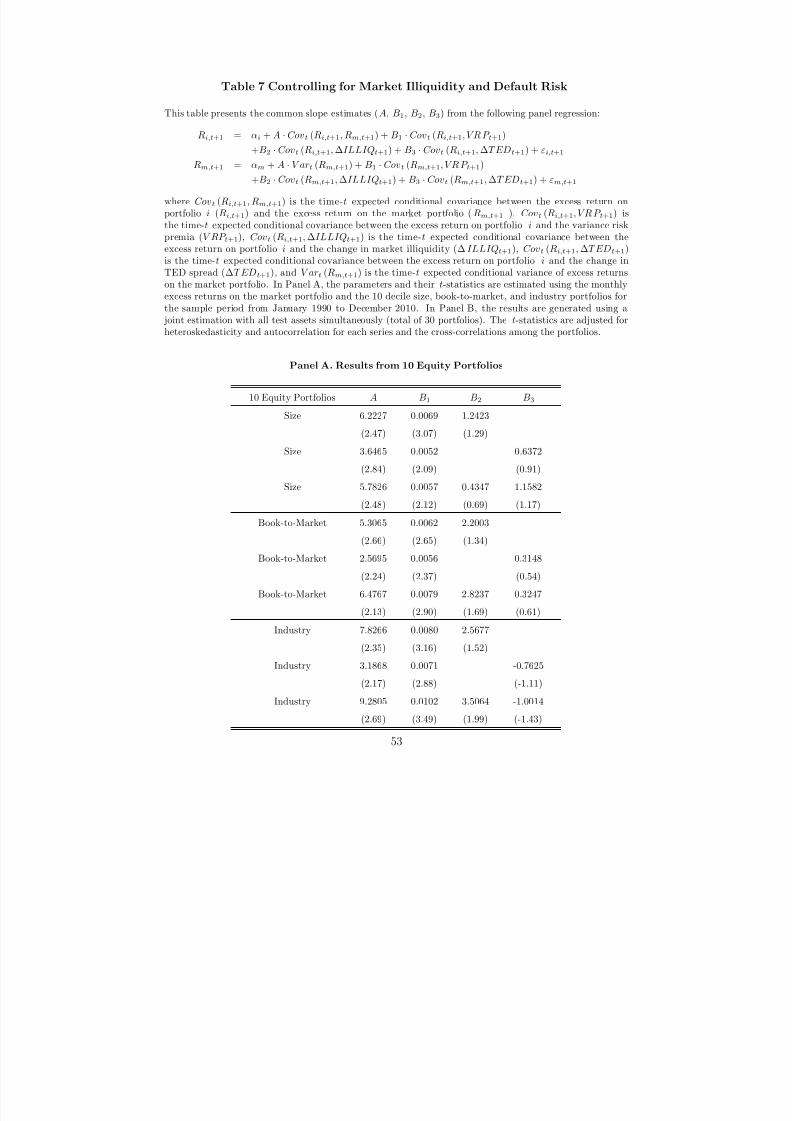
7/31/2019 Risk Uncertainty and Return
http://slidepdf.com/reader/full/risk-uncertainty-and-return 56/75
Table 7 Controlling for Market Illiquidity and Default Risk
This table presents the common slope estimates (A, B1, B2, B3) from the following panel regression:
Ri,t+1 = αi + A · Covt (Ri,t+1, Rm,t+1) + B1 · Covt (Ri,t+1, V R P t+1)
+B2 · Covt (Ri,t+1, ∆ILLIQt+1) + B3 · Covt (Ri,t+1, ∆T EDt+1) + εi,t+1Rm,t+1 = αm + A · V art (Rm,t+1) + B1 · Covt (Rm,t+1, V R P t+1)
+B2 · Covt (Rm,t+1, ∆ILLIQt+1) + B3 · Covt (Rm,t+1, ∆T EDt+1) + εm,t+1
where Covt (Ri,t+1, Rm,t+1) is the time-t expected conditional covariance between the excess return onportfolio i (Ri,t+1) and the excess return on the market portfolio (Rm,t+1 ), Covt (Ri,t+1, V R P t+1) isthe time-t expected conditional covariance between the excess return on portfolio i and the variance riskpremia (V RP t+1), Covt (Ri,t+1, ∆ILLIQt+1) is the time-t expected conditional covariance between theexcess return on portfolio i and the change in market illiquidity (∆ILLIQt+1), Covt (Ri,t+1, ∆T EDt+1)is the time-t expected conditional covariance between the excess return on portfolio i and the change inTED spread (∆T EDt+1), and V art (Rm,t+1) is the time-t expected conditional variance of excess returnson the market portfolio. In Panel A, the parameters and their t-statistics are estimated using the monthlyexcess returns on the market portfolio and the 10 decile size, book-to-market, and industry portfolios forthe sample period from January 1990 to December 2010. In Panel B, the results are generated using a
joint estimation with all test assets simultaneously (total of 30 portfolios). The t-statistics are adjusted forheteroskedasticity and autocorrelation for each series and the cross-correlations among the portfolios.
Panel A. Results from 10 Equity Portfolios
10 Equity Portfolios A B1 B2 B3
Size 6.2227 0.0069 1.2423
(2.47) (3.07) (1.29)
Size 3.6465 0.0052 0.6372(2.84) (2.09) (0.91)
Size 5.7826 0.0057 0.4347 1.1582
(2.48) (2.12) (0.69) (1.17)
Book-to-Market 5.3065 0.0062 2.2003
(2.66) (2.65) (1.34)
Book-to-Market 2.5695 0.0056 0.3148
(2.24) (2.37) (0.54)
Book-to-Market 6.4767 0.0079 2.8237 0.3247
(2.13) (2.90) (1.69) (0.61)
Industry 7.8266 0.0080 2.5677
(2.35) (3.16) (1.52)
Industry 3.1868 0.0071 -0.7625
(2.17) (2.88) (-1.11)
Industry 9.2805 0.0102 3.5064 -1.0014
(2.69) (3.49) (1.99) (-1.43)
53

7/31/2019 Risk Uncertainty and Return
http://slidepdf.com/reader/full/risk-uncertainty-and-return 57/75
Table 7 (continued)
Panel B. Results from 30 Equity Portfolios
A B1 B2 B3
2.3110 0.0053
(2.64) (3.72)
3.2552 0.0060 0.6796
(2.82) (4.03) (1.94)
2.1153 0.0055 -0.0477
(2.41) (3.49) (-0.11)
3.0967 0.0062 0.6497 -0.0844
(2.72) (3.78) (1.95) (-0.20)
54

7/31/2019 Risk Uncertainty and Return
http://slidepdf.com/reader/full/risk-uncertainty-and-return 58/75
Table 8 Long-Short Equity Portfolios Sorted by VRP-beta
Quintile portfolios are formed every month from January 1990 to December 2010 by sorting the 25 and 100Size/BM portfolios based on their VRP-beta (V RP beta) over the past one month. Quintile 1 (Q1) is theportfolio of Size/BM portfolios with the lowest V RP beta over the past one month. Quintile 5 (Q5) is theportfolio of Size/BM portfolios with the highest V RP beta over the past one month. The table reports theaverage excess monthly returns and the 3-factor Fama-French alphas (FF3 alpha) on the VRP-beta sortedportfolios. The last row presents the differences in monthly returns and the differences in alphas with respectto the 3-factor Fama-French model between Quintiles 5 and 1 and the corresponding t-statistics. Average
excess return and risk-adjusted returns are given in percentage terms. Newey-West (1987) t-statistics arereported in parentheses.
25 Size/BM Portfolios 100 Size/BM Portfolios
Average Excess Return FF3 Alpha Average Excess Return FF3 Alpha
Q1 0.0038 -0.0042 Q1 0.0048 -0.0037
(1.08) (-2.66) (1.33) (-2.61)
Q2 0.0074 -0.0005 Q2 0.0072 -0.0008
(2.49) (-0.60) (2.40) (-0.94)
Q3 0.0078 0.0002 Q3 0.0080 0.0004
(2.72) (0.24) (2.75) (0.62)
Q4 0.0097 0.0022 Q4 0.0094 0.0019
(3.26) (1.80) (3.25) (2.15)
Q5 0.0096 0.0027 Q5 0.0097 0.0028
(3.47) (2.46) (3.30) (2.10)
Q5-Q1 0.0058 0.0069 Q5-Q1 0.0049 0.0065
(2.51) (3.33) (2.14) (2.70)
55
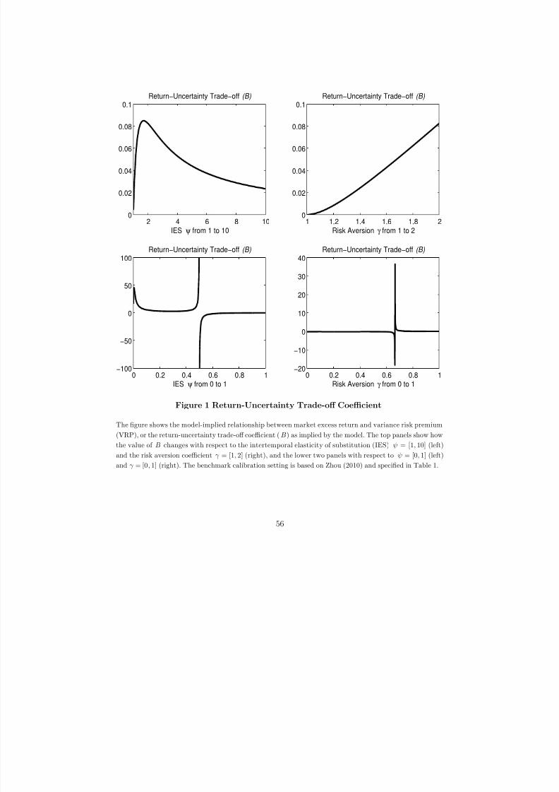
7/31/2019 Risk Uncertainty and Return
http://slidepdf.com/reader/full/risk-uncertainty-and-return 59/75
2 4 6 8 100
0.02
0.04
0.06
0.08
0.1
IES ψ from 1 to 10
Return−Uncertainty Trade−off (B)
0 0.2 0.4 0.6 0.8 1−100
−50
0
50
100
IES ψ from 0 to 1
Return−Uncertainty Trade−off (B)
1 1.2 1.4 1.6 1.8 20
0.02
0.04
0.06
0.08
0.1
Risk Aversion γ from 1 to 2
Return−Uncertainty Trade−off (B)
0 0.2 0.4 0.6 0.8 1−20
−10
0
10
20
30
40
Risk Aversion γ from 0 to 1
Return−Uncertainty Trade−off (B)
Figure 1 Return-Uncertainty Trade-off Coefficient
The figure shows the model-implied relationship between market excess return and variance risk premium(VRP), or the return-uncertainty trade-off coefficient (B) as implied by the model. The top panels show how
the value of B changes with respect to the intertemporal elasticity of substitution (IES) ψ = [1, 10] (left)
and the risk aversion coefficient γ = [1, 2] (right), and the lower two panels with respect to ψ = [0, 1] (left)
and γ = [0, 1] (right). The benchmark calibration setting is based on Zhou (2010) and specified in Table 1.
56

7/31/2019 Risk Uncertainty and Return
http://slidepdf.com/reader/full/risk-uncertainty-and-return 60/75
Jan90 Jan92 Jan94 Jan96 Jan98 Jan00 Jan02 Jan04 Jan06 Jan08 Jan10−50
0
50
100
150
200
250S&P500 Variance Risk Premium
Jan90 Jan92 Jan94 Jan96 Jan98 Jan00 Jan02 Jan04 Jan06 Jan08 Jan100
50
100
150
200
250
300S&P500 Implied Variance
Jan90 Jan92 Jan94 Jan96 Jan98 Jan00 Jan02 Jan04 Jan06 Jan08 Jan100
50
100
150
200
250
300S&P500 Expected Variance
Figure 2 Variance Risk Premium, Implied and Realized Variances
This figure plots variance risk premium or the implied-expected variance difference (top panel), implied
variance (middle panel), and forecasted realized variance (bottom panel) for the S&P500 market index from
January 1990 to December 2010. The variance risk premium is based on the realized variance forecast from
lagged implied and realized variances. The shaded areas represent NBER recessions.
57

7/31/2019 Risk Uncertainty and Return
http://slidepdf.com/reader/full/risk-uncertainty-and-return 61/75
Q3−92 Q1−95 Q3−97 Q1−00 Q3−02 Q1−05 Q3−07 Q1−10
−4
−2
0
2
4
Variance Risk Premium and GDP Growth (Standardized)
Variance Risk Premium
GDP Growth
Figure 3 Variance Risk Premium and GDP Growth
The figure plots the GDP growth rates (thin line) together with the variance risk premium (thick line) from
1990Q1 to 2010Q4. Both of the series are standardized to have mean zero and variance one. The shaded
areas represent NBER recessions.
58

7/31/2019 Risk Uncertainty and Return
http://slidepdf.com/reader/full/risk-uncertainty-and-return 62/75
Small 2 3 4 5 6 7 8 9 Big
0.5
0.6
0.7
0.8
Realized and Expected Returns on Size Portfolios
P e r c e n t a g e R e t u r n s
Realized Returns
Expected Returns from Conditional ICAPM with VRP
Expected Returns from Conditional CAPM
Growth 2 3 4 5 6 7 8 9 Value
0.5
0.55
0.6
0.65
0.7
0.75
0.8
0.85
Realized and Expected Returns on Book−to−Market Portfolios
P e r c e n t a g e R e t u r n s
Realized Returns
Expected Returns from Conditional ICAPM with VRP
Expected Returns from Conditional CAPM
Telcm Utils Other Durbl Shops Hlth NoDur Manuf Enrgy HiTec
0.3
0.4
0.5
0.6
0.7
0.8
Realized and Expected Returns on Industry Portfolios
P e r c e n t a g e R e t u r n s
Realized Returns
Expected Returns from Conditional ICAPM with VRP
Expected Returns from Conditional CAPM
Figure 4 Relative Performance of the Conditional ICAPM with Uncertainty
This figure plots the realized monthly average excess returns on the size (top panel), book-to-market (middle
panel), and industry portfolios (bottom panel) and the cross-section of expected excess returns generated
by the Conditional CAPM with the market factor and the Conditional ICAPM with the market and VRP
factors. The results indicate superior performance of the conditional asset pricing model introduced in the
paper.
59

7/31/2019 Risk Uncertainty and Return
http://slidepdf.com/reader/full/risk-uncertainty-and-return 63/75
Risk, Uncertainty, and Expected
Returns—Internet AppendixTuran G. Bali∗and Hao Zhou†
∗Turan G. Bali is the Dean’s Research Professor of Finance, Department of Finance, McDonoughSchool of Business, Georgetown University, Washington, D.C. 20057. Phone: (202) 687-5388, E-mail:[email protected].
†Hao Zhou is a senior economist with the Risk Analysis Section, Division of Research and Statis-tics, Federal Reserve Board, Mail Stop 91, Washington, D.C. 20551. Phone: (202) 452-3360, E-mail:[email protected].

7/31/2019 Risk Uncertainty and Return
http://slidepdf.com/reader/full/risk-uncertainty-and-return 64/75
A Equity Portfolios
In addition to the 1990-2010 period, Table I presents the monthly raw return and CAPM
Alpha differences between high-return (long) and low-return (short) equity portfolios (size,
book-to-market, and industry) for the sample periods 1926-2010 and 1963-2010. For the
sample period July 1926 – December 2010, the average return difference between the Small
and Big portfolios is 0.60% per month with the OLS t-statistic of 2.49 and the Newey-West
(1987) t-statistic of 2.36, implying that small stocks on average generate higher returns
than big stocks. The CAPM Alpha (or abnormal return) for the long-short size portfolio
is 0.27% per month with the OLS t-statistic of 1.22 and the Newey-West t-statistic of 1.38.
This economically and statistically insignificant Alpha indicates that the static CAPM does
explain the size effect for the 1926-2010 period.
For the ten book-to-market portfolios, the average return difference between the Value
and Growth portfolios is 0.53% per month with the OLS t-statistic of 2.52 and the Newey-
West t-statistic of 2.46, implying that value stocks on average generate higher returns than
growth stocks (the so-called value premium). Similar to our findings for the size portfolios,
the unconditional CAPM can explain the value premium for the 1926-2010 period; the CAPM
Alpha (or abnormal return) for the long-short book-to-market portfolio is only 0.24% permonth with the OLS t-statistic of 1.25 and the Newey-West t-statistic of 1.26.
The last six rows in Table I report average return differences and CAPM Alphas for
the industry portfolios (10-, 17-, 30-, 38-, 48-, and 49-industry portfolios). For the long
sample period of 1926-2010, only the extreme portfolios of 48 and 49 industries generate
significant return differences, whereas the average return differences for the high-return and
low-return portfolios of 10, 17, 30, and 38 industries are either statistically insignificant
or marginally significant. For 48- and 49-industry portfolios of Kenneth French, “Aero”
industry has the highest average monthly return, whereas “Other” industry has the lowest
return, yielding an average monthly return difference of 66 basis points with the Newey-West
t-statistic of 2.55.1 More importantly, the static CAPM cannot explain the industry effect;
1According to the 48- and 49-industry definitions and four-digit SIC codes reported at Kenneth French’sonline data library, “Aero” industry includes Aircraft & parts (3720-3720), Aircraft (3721-3721), Aircraft
2
7/31/2019 Risk Uncertainty and Return
http://slidepdf.com/reader/full/risk-uncertainty-and-return 65/75
the CAPM alpha (or abnormal return) for the “Aero-Other” arbitrage portfolio is 0.50%
per month and statistically significant with the t-statistic of 2.04. Although the average
return differences between high-return and low-return portfolios of 30 and 38 industries
are marginally significant, the CAPM Alphas are found to be significant. For 30-industryportfolios, the average return difference between “Coal” and “Other” industries is 0.51% per
month and marginally significant with the t-statistic of 1.71.2 However, the CAPM Alpha
for the “Coal-Other” arbitrage portfolio is 0.65% per month with the t-statistic of 2.28. For
38-industry portfolios, the average return difference between “Oil” and “Whlsl” industries
is 0.42% per month and marginally significant with the t-statistic of 1.85.3 However, the
CAPM Alpha for the “Oil-Whlsl” arbitrage portfolio is 0.49% per month with the t-statistic
of 2.06.
Fama and French (1992) identify economically and statistically significant value premium
for the post-1963 period. Moreover, Fama and French (1992) find that the post-1963 value
premium is not explained by the CAPM. However, Ang and Chen (2007) provide evidence
that the value premium is captured by the CAPM for the sample period of 1926-1963. They
also show that the conditional CAPM with stochastic betas can explain the return differences
between value and growth portfolios even for the post-1963 period. Fama and French (2006)
indicate that the performance of the CAPM with regard to the book-to-market effect varies
across subperiods. We investigate the significance of size, book-to-market, and industry
effects for the sample that generated heated debate on value premium. We compute the
average return differences and Alphas for the subsample period of July 1963 – December
2010.
As presented in Table I, the average return difference between the Small and Big port-
engines, engine parts (3723-3724), Aircraft parts (3725-3725), and Aircraft parts (3728-3729). “Other”
industry includes Sanitary services (4950-4959), Steam, air conditioning supplies (4960-4961), Irrigationsystems (4970-4971), and Cogeneration - SM power producer (4990-4991).
2According to the 30-industry definitions and four-digit SIC codes reported at Kenneth French’s onlinedata library, “Coal” industry includes Bituminous coal (1200-1299). “Other” industry includes Sanitaryservices (4950-4959), Steam, air conditioning supplies (4960-4961), Irrigation systems (4970-4971), and Co-generation - SM power producer (4990-4991).
3According to the 38-industry definitions and four-digit SIC codes reported at Kenneth French’s onlinedata library, “Oil” industry includes Oil and Gas Extraction (1300-1399) and “Whlsl” industry includesWholesale (5000-5199).
3

7/31/2019 Risk Uncertainty and Return
http://slidepdf.com/reader/full/risk-uncertainty-and-return 66/75
folios as well as the CAPM Alpha for “Small-Big” arbitrage portfolio are positive, but they
are economically and statistically insignificant, indicating that the size effect disappears
for the post-1963 period. Similar to the findings of Ang and Chen (2007) and Fama and
French (2006), value premium remains economically and statistically significant for the sam-ple period July 1963 – December 2010; the average raw and risk-adjusted return differences
between the Value and Growth portfolios is 0.55% per month and statistically significant,
implying that value stocks on average generate higher returns than growth stocks and this
value premium cannot be explained by the static CAPM.
The results for the industry portfolios are similar for the post-1963 period. The high-
return and low-return portfolios of 30 and 38 industries generate marginally significant, 48
and 49 industries generate significant return differences, whereas the average return differ-
ences for the high-return and low-return portfolios of 10 and 17 industries are insignificant.
Specifically, for 30-, 48- and 49-industry portfolios of Kenneth French, “Coal” industry has
the highest average monthly return, whereas “Other” industry has the lowest return, yield-
ing an average raw and risk-adjusted return differences of 79 to 92 basis points per month
and statistically significant. The unconditional CAPM cannot explain these industry ef-
fects either. For 38-industry portfolios, the average return and Alpha differences between
“Smoke” and “Govt” industries are about 1.06% and 1.07% per month and significant with
the Newey-West t-statistics of 2.61 and 2.69, respectively.4
B DCC Model of Engle (2002)
We estimate the conditional covariances of each equity portfolio with the market portfolio
and V RP (σim,t+1 , σi,V RP,t+1 ) based on the mean-reverting DCC model of Engle (2002).
Engle defines the conditional correlation between two random variables r1 and r2 that each4According to the 38-industry definitions and four-digit SIC codes reported at Kenneth French’s online
data library, “Smoke” industry includes Tobacco Products (2100-2199) and “Govt” industry includes PublicAdministration (9000-9999).
4

7/31/2019 Risk Uncertainty and Return
http://slidepdf.com/reader/full/risk-uncertainty-and-return 67/75
has zero mean as
ρ12,t =E t−1 (r1,t · r2,t)
E t−1
r2
1,t
· E t−1
r2
1,t
, (A1)
where the returns are defined as the conditional standard deviation times the standardized
disturbance:
σ2i,t = E t−1
r2
i,t
, ri,t = σi,t · ui,t, i = 1, 2 (A2)
where ui,t is a standardized disturbance that has zero mean and variance one for each series.
Equations (A1) and (A2) indicate that the conditional correlation is also the conditional
covariance between the standardized disturbances:
ρ12,t = E t−1 (u1,t · u2,t) E t−1
u2
1,t
· E t−1
u2
1,t
= E t−1 (u1,t · u2,t) . (A3)
The conditional covariance matrix of returns is defined as
H t = Dt · ρt · Dt, where Dt = diag
σ2i,t
, (A4)
where ρt is the time-varying conditional correlation matrix
E t−1 (ut
·u′
t) = D−1t
·H t
·D−1
t = ρt, where ut = D−1t
·rt. (A5)
Engle (2002) introduces a mean-reverting DCC model:
ρij,t =qij,t√
qii,t · q jj,t, (A6)
qij,t = ρij + a1 · (ui,t−1 · u j,t−1 − ρij) + a2 · (qij,t−1 − ρij ) (A7)
where ρij is the unconditional correlation between ui,t and u j,t. Equation (A7) indicates that
the conditional correlation is mean reverting towards ρij as long as a1 + a2 < 1.
Engle (2002) assumes that each asset follows a univariate GARCH process and writes
the log likelihood function as:
L = −1
2
T t=1
n log(2π) + log |H t| + r′
tH −1t rt
= −1
2
T t=1
n log(2π) + 2 log |Dt| + r′
tD−1t D−1
t rt − u′
tut + log |ρt| + u′
tρ−1t ut
. (A8)
5

7/31/2019 Risk Uncertainty and Return
http://slidepdf.com/reader/full/risk-uncertainty-and-return 68/75
As shown in Engle (2002), letting the parameters in Dt be denoted by θ and the additional
parameters in ρt be denoted by ϕ, equation (A8) can be written as the sum of a volatility
part and a correlation part:
L(θ, ϕ) = LV (θ) + LC (θ, ϕ). (A9)
The volatility term is
LV (θ) = −1
2
T t=1
n log(2π) + log |Dt|2 + r′
tD−2t rt
, (A10)
and the correlation component is
LC (θ, ϕ) = −1
2
T
t=1
log |ρt| + u
′
tρ
−1
t ut − u
′
tut
. (A11)
The volatility part of the likelihood is the sum of individual GARCH likelihoods:
LV (θ) = −1
2
T t=1
ni=1
log(2π) + log
σ2
i,t
+
r2i,t
σ2i,t
, (A12)
which is jointly maximized by separately maximizing each term. The second part of the like-
lihood is used to estimate the correlation parameters. The two-step approach to maximizing
the likelihood is to find
θ = arg maxLV (θ), (A13)
and then take this value as given in the second stage:
ϕ = arg maxLC (θ, ϕ). (A14)
C System of Regression Equations
Consider a system of n equations, of which the typical ith equation is
yi = X iβi + ui, (A15)
where yi is a N × 1 vector of time-series observations on the ith dependent variable, X i is a
N × ki matrix of observations of ki independent variables, βi is a ki × 1 vector of unknown
6

7/31/2019 Risk Uncertainty and Return
http://slidepdf.com/reader/full/risk-uncertainty-and-return 69/75
coefficients to be estimated, and ui is a N ×1 vector of random disturbance terms with mean
zero. Parks (1967) proposes an estimation procedure that allows the error term to be both
serially and cross-sectionally correlated. In particular, he assumes that the elements of the
disturbance vector u follow an AR(1) process:
uit = ρuit−1 + εit; ρi < 1, (A16)
where εit is serially independently but contemporaneously correlated:
Cov (εitε jt) = σij , for any i,j, and Cov (εitε js) = 0, for s = t (A17)
Equation (A15) can then be written as
yi = X iβi + P iui, (A18)
with
P i =
(1 − ρ2i )
−1/20 0 ... 0
ρi (1 − ρ2i )
−1/21 0 ... 0
ρ2i (1 − ρ2
i )−1/2
ρ 1 ... 0.
.
.
ρN −1
i(1−
ρ2
i)−1/2
ρN −2 ρN −3 ... 1
. (A19)
Under this setup, Parks (1967) presents a consistent and asymptotically efficient three-
step estimation technique for the regression coefficients. The first step uses single equation
regressions to estimate the parameters of autoregressive model. The second step uses single
equation regressions on transformed equations to estimate the contemporaneous covariances.
Finally, the Aitken estimator is formed using the estimated covariance,
β = X T Ω−1X −1
X T Ω−1y, (A20)
where Ω ≡ E [uuT ] denotes the general covariance matrix of the innovation. In our applica-
tion, we use the aforementioned methodology with the slope coefficients restricted to be the
same for all equity portfolios and individual stocks. In particular, we use the same three-step
procedure and the same covariance assumptions as in equations (A16) to (A19) to estimate
the covariances and to generate the t-statistics for the parameter estimates.
7

7/31/2019 Risk Uncertainty and Return
http://slidepdf.com/reader/full/risk-uncertainty-and-return 70/75
D DCC with Asymmetric GARCH
Because the conditional variance and covariance of stock market returns are not observable,
different approaches and specifications used in estimating the conditional variance and co-
variance could lead to different conclusions. We have so far used the bivariate GARCH(1,1)
model of Bollerslev (1986) in equations (18)-(19) and (24)-(25) to obtain conditional variance
and covariance estimates. In this section, we investigate whether changing these specifica-
tions influences our main findings.
The current volatility in the GARCH(1,1) model is defined as a symmetric, linear function
of the last period’s unexpected news and the last period’s volatility. Since, in a symmetric
GARCH process, positive and negative information shocks of the same magnitude produce
the same amount of volatility, the symmetric GARCH model cannot cope with the skewness
of stock return distribution. If a negative return shock causes more volatility than a positive
return shock of the same size, the symmetric GARCH model underpredicts the amount
of volatility following negative shocks and overpredicts the amount of volatility following
positive shocks. Furthermore, if large return shocks cause more volatility than a quadratic
function allows, then the symmetric GARCH model underpredicts volatility after a large
return shock and overpredicts volatility after a small return shock.In this section we use an asymmetric GARCH model of Glosten, Jagannathan, and
Runkle (1993) that explicitly takes account of skewed distributions and allows good news
and bad news to have different impacts on the conditional volatility forecasts. To test whether
such variations in the variance forecasting specification alter our conclusion, we re-estimate
the DCC-based conditional covariances using the following alternative specification:
Ri,t+1 = αi0 + αi
1Ri,t + εi,t+1
Rm,t+1 = αm0 + α
m1 Rm,t + εm,t+1
V RP t+1 = αV RP 0 + αV RP
1 V RP t + εV RP,t+1
E t
ε2i,t+1
≡ σ2i,t+1 = βi
0 + βi1ε2
i,t + βi2σ2
i,t + βi3ε2
i,tD−
i,t
E t
ε2m,t+1
≡ σ2m,t+1 = βm
0 + βm1 ε2
m,t + βm2 σ2
m,t + βm3 ε2
m,tD−
m,t
E t
ε2V RP,t+1
≡ σ2V RP,t+1 = βV RP
0 + βV RP 1 ε2
V RP,t + βV RP 2 σ2
V RP,t + βV RP 3 ε2
V RP,tD−
V RP,t
E t [εi,t+1εm,t+1] ≡ σim,t+1 = ρim,t+1 · σi,t+1 · σm,t+1
E t [εi,t+1εV RP,t+1] ≡ σi,V RP,t+1 = ρi,V RP,t+1 · σi,t+1 · σV RP,t+1
E t [εm,t+1εV RP,t+1] ≡ σm,V RP,t+1 = ρm,V RP,t+1 · σm,t+1 · σV RP,t+1
(A21)
8

7/31/2019 Risk Uncertainty and Return
http://slidepdf.com/reader/full/risk-uncertainty-and-return 71/75
where D−
i,t, D−
m,t, and D−
V RP,t are indicator functions that equals one when εi,t+1, εm,t+1, and
εV RP,t+1 are negative and zero otherwise. The indicator function generates an asymmetric
GARCH effect between positive and negative shocks. ρim,t+1, ρi,V RP,t+1, and ρm,V RP,t+1 are
the time-t expected conditional correlations estimated using the mean-reverting DCC modelof Engle (2002).
A notable point in Table II is that the main findings from an asymmetric GARCH
specification of the conditional covariances are very similar to those reported in Table 2.
Specifically, the risk aversion coefficients are estimated to be positive and highly significant
for all equity portfolios; A is in the range of 2.53 to 3.54 with the t-statistics ranging from
2.58 to 3.11, implying a significantly positive link between expected return and risk. Sim-
ilar to our results from GARCH(1,1) specification, asymmetric GARCH model of Glosten,
Jagannathan, and Runkle (1993) yields positive and significant coefficient estimates on the
covariance between equity portfolios and the variance risk premia. Specifically, the uncer-
tainty aversion coefficients (B) are in the range of 0.0054 to 0.0075 with the t-statistics
between 2.68 and 3.30. These results show that equity portfolios that are highly correlated
with uncertainty (proxied by VRP) carry a significant premium relative to portfolios that
are uncorrelated or lowly correlated with VRP.
With this alternative covariance specification, we also examine the empirical validity of
the conditional asset pricing model by testing the joint hypothesis. As shown in Table II,
the Wald1 statistics for the size, book-to-market, and industry portfolios are, respectively,
16.91, 7.89, and 14.41 with the corresponding p-values of 0.11, 0.72, and 0.21. The signifi-
cantly positive risk and uncertainty aversion coefficients and the insignificant Wald1 statistics
indicate that the two-factor model explains the time-series and cross-sectional variation in
equity portfolios. Finally, we investigate whether the model with asymmetric GARCH spec-
ification explains the return spreads between Small and Big; Value and Growth; and HiTec
and Telcm portfolios. The last row in Table II reports Wald2 statistics from testing the
equality of conditional alphas for high-return and low-return portfolios (H 0 : α1 = α10). For
the size, book-to-market, and industry portfolios, the Wald2 statistics provide no evidence
for a significant conditional alpha for “Small-Big”, “Value-Growth”, and “HiTec-Telcm”
9

7/31/2019 Risk Uncertainty and Return
http://slidepdf.com/reader/full/risk-uncertainty-and-return 72/75
arbitrage portfolios. Overall, the DCC-based conditional covariances from the asymmet-
ric GARCH model captures the time-series and cross-sectional variation in returns on size,
book-to-market, and industry portfolios and generates significantly positive risk-return and
uncertainty-return tradeoffs.
10

7/31/2019 Risk Uncertainty and Return
http://slidepdf.com/reader/full/risk-uncertainty-and-return 73/75
References
Ang, Andrew and Joseph Chen (2007), “CAPM Over the Long-Run: 1926-2001,” Journal
of Empirical Finance, vol. 14, 1–40.
Bollerslev, Tim (1986), “Generalized Autoregressive Conditional Heteroskedasticity,” Jour-nal of Econometrics , vol. 31, 307–327.
Engle, Robert F. (2002), “Dynamic Conditional Correlation: a Simple Class of Multivariate
Generalized Autoregressive Conditional Heteroskedasticity Models,” Journal of Business
and Economic statistics , vol. 20, 339–350.
Fama, Eugene F. and Kenneth R. French (1992), “The Cross-Section of Expected Stock
Returns,” Journal of Finance, vol. 47, 427–465.
Fama, Eugene F. and Kenneth R. French (2006), “The Value Premium and the CAPM,”Journal of Finance, vol. 61, 2137–2162.
Glosten, Larry R., Ravi Jagannathan, and David Runkle (1993), “On the Relation between
the Expected Value and the Volatility of the Nominal Excess Return on Stocks,” Journal
of Finance, vol. 48, 1779–1801.
Parks, Richard W. (1967), “Efficient Estimation of a System of Regression Equations when
Disturbances are both Serially and Contemporaneously Correlated,” Journal of the Amer-
ican Statistical Association , vol. 62, 500–509.
11
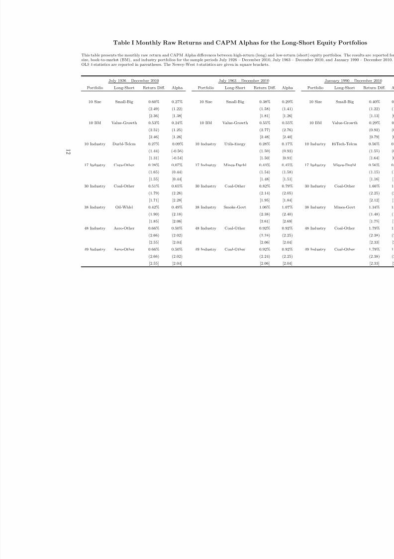
7/31/2019 Risk Uncertainty and Return
http://slidepdf.com/reader/full/risk-uncertainty-and-return 74/75
Table I Monthly Raw Returns and CAPM Alphas for the Long-Short Equi
This table presents the monthly raw return and CAPM Alpha differences between high-return (long) and low-return (short) equity porsize, book-to-market (BM), and industry portfolios for the sample periods July 1926 – December 2010, July 1963 – December 2010, anOLS t-statistics are reported in parentheses. The Newey-West t-statistics are given in square brackets.
July 1926 – December 2010 July 1963 – December 2010 Jan
Portfolio Long-Short Return Diff. Alpha Portfolio Long-Short Return Diff. Alpha Portfolio
10 Size Small-Big 0.60% 0.27% 10 Size Small-Big 0.38% 0.29% 10 Size
(2.49) (1.22) (1.58) (1.41)
[2.36] [1.38] [1.81] [1.26]
10 BM Value-Growth 0.53% 0.24% 10 BM Value-Growth 0.55% 0.55% 10 BM
(2.52) (1.25) (2.77) (2.76)
[2.46] [1.26] [2.48] [2.40]
10 Industry Durbl-Telcm 0.27% -0.09% 10 Industry Utils-Enrgy 0.28% 0.17% 10 Industry
(1.44) (-0.56) (1.50) (0.93)
[1.31] [-0.54] [1.50] [0.91]
17 Industry Cars-Other 0.28% 0.07% 17 Industry Mines-Durbl 0.43% 0.45% 17 Industry
(1.65) (0.44) (1.54) (1.58)
[1.55] [0.44] [1.48] [1.51]
30 Industry Coal-Other 0.51% 0.65% 30 Industry Coal-Other 0.82% 0.79% 30 Industry
(1.79) (2.26) (2.14) (2.05)
[1.71] [2.28] [1.95] [1.84]
38 Industry Oil-Whlsl 0.42% 0.49% 38 Industry Smoke-Govt 1.06% 1.07% 38 Industry
(1.90) (2.18) (2.38) (2.40)
[1.85] [2.06] [2.61] [2.69]
48 Industry Aero-Other 0.66% 0.50% 48 Industry Coal-Other 0.92% 0.92% 48 Industry
(2.66) (2.02) (2.24) (2.25)
[2.55] [2.04] [2.06] [2.04]
49 Industry Aero-Other 0.66% 0.50% 49 Industry Coal-Other 0.92% 0.92% 49 Industry
(2.66) (2.02) (2.24) (2.25)
[2.55] [2.04] [2.06] [2.04]
1 2

7/31/2019 Risk Uncertainty and Return
http://slidepdf.com/reader/full/risk-uncertainty-and-return 75/75
Table II Results from Asymmetric GARCH Model
This table reports the portfolio-specific intercepts and the common slope estimates from the following panel regression:
Ri,t+1 = αi + A · Covt (Ri,t+1, Rm,t+1) + B · Covt (Ri,t+1, V RP t+1) + εi,t+1
Rm,t+1 = αm + A·
V art (Rm,t+1) + B·
Covt (Rm,t+1, V RP t+1) + εm,t+1
where the conditional variance and covariances are estimated using the asymmetric GARCH model of Glosten, Jagannathan,and Runkle (1993). The parameters and their t-statistics are estimated using the monthly excess returns on the marketportfolio and the ten decile size, book-to-market, and industry portfolios for the sample period from January 1990 to December2010. The alphas (αi) are reported for each equity portfolio and the t-statistics are presented in parentheses. The t-statisticsare adjusted for heteroskedasticity and autocorrelation for each series and cross-correlations among the portfolios. The lastfour rows, respectively, show the common slope coefficients (A and B), the Wald1 statistics from testing the joint hypothesisH 0 : α1 = α2 = ...αm = 0 , and the Wald2 statistics from testing the equality of Alphas for high-return and low-returnportfolios (Small vs. Big; Value vs. Growth; and HiTec vs. Telcm). The p-values of Wald1 and Wald2 statistics are given insquare brackets.
Size αi, αm BM αi, αm Industry αi, αm
Small 0.0052 Growth 0.0035 NoDur 0.0051
(1.23) (0.87) (1.94)
2 0.0037 2 0.0047 Durbl 0.0028
(0.85) (1.35) (0.57)
3 0.0040 3 0.0052 Manuf 0.0055
(0.99) (1.55) (1.61)
4 0.0030 4 0.0064 Enrgy 0.0064
(0.75) (1.85) (1.85)
5 0.0038 5 0.0056 HiTec 0.0029
(0.97) (1.71) (0.52)
6 0.0037 6 0.0050 Telcm 0.0004
(1.05) (1.48) (0.11)
7 0.0041 7 0.0057 Shops 0.0036(1.19) (1.76) (1.04)
8 0.0034 8 0.0058 Hlth 0.0043
(0.97) (1.74) (1.37)
9 0.0036 9 0.0066 Utils 0.0042
(1.11) (1.92) (1.58)
Big 0.0012 Value 0.0081 Other 0.0030
(0.38) (1.88) (0.81)
Market 0.0018 Market 0.0033 Market 0.0028
(0.57) (1.20) (0.82)
A 3.2927 A 2.5303 A 3.5369