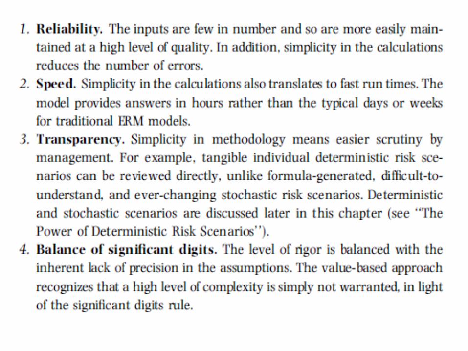
Risk Quantification

Any intelligent fool can invent further complications, but it takes a genius to retain, or recapture, simplicity. E.F. Schumacher

THE RISK QUANTIFICATION ERM process step is the lynchpin of the ERM process cycle. It enhances the key risk ranking and prioritization performed in the prior ERM process step—risk identification—and it also provides the information necessary to perform the next ERM process step—risk decision making. The key linkage performed in this step is the connection of risk and value by quantifying risk in terms of its value impact. This is the bridge between risk and return.

PRACTICAL MODELINGThe single most important characteristic of the value-based ERM model is that it is practical. All aspects of the model—inputs, calculations, and outputs—are kept simple, with the sole purpose, constantly in mind, of supporting decision making.

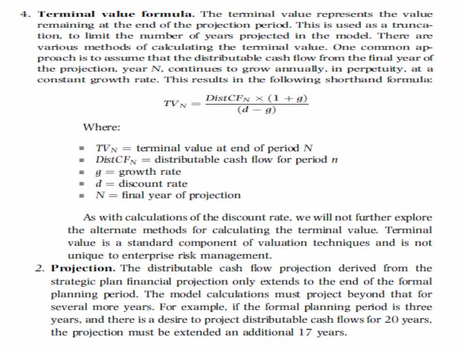
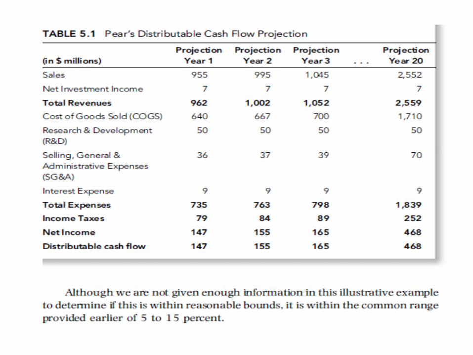
Input of Data and AssumptionsThe data and assumptions needed to calculate the enterprise baseline value include the following three items:1. Strategic plan financial projection. The first item needed as input for the calculation of the baseline company value is the strategic plan financial projection. This is a financial projection that extends out to the end of the formal planning period; for example, a three-year period. This should include the latest version of the official strategic plan projection as well as any detailed supporting documents. This should also include any informationavailable internally regarding projections or expectations beyond the formal planning period; this is often limited to additional revenue growth, expense reduction, and known or scheduled changes in investments.

Recent financials. The second item needed as input for the calculation of the baseline company value is recent financial results that are normalized for any one-time or anomalous items. This includes the income statement, balance sheet, cash flow statement, and, for financial services companies, required capital calculations. In addition, this includes the detailed data supporting the construction of the financials; for example, rates of returns on invested assets, tax rates, and so forth

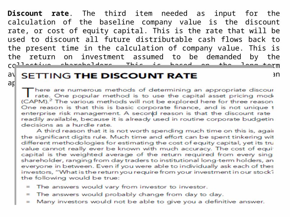
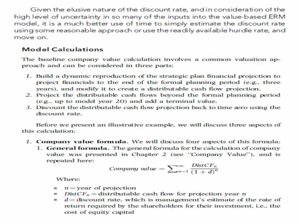
Discount rate. The third item needed as input for the calculation of the baseline company value is the discount rate, or cost of equity capital. This is the rate that will be used to discount all future distributable cash flows back to the present time in the calculation of company value. This is the return on investment assumed to be demanded by the collective shareholders. This is based on the long-term average required return. For a discussion on determining an appropriate discount rate, see ‘‘Setting the Discount Rate.’’

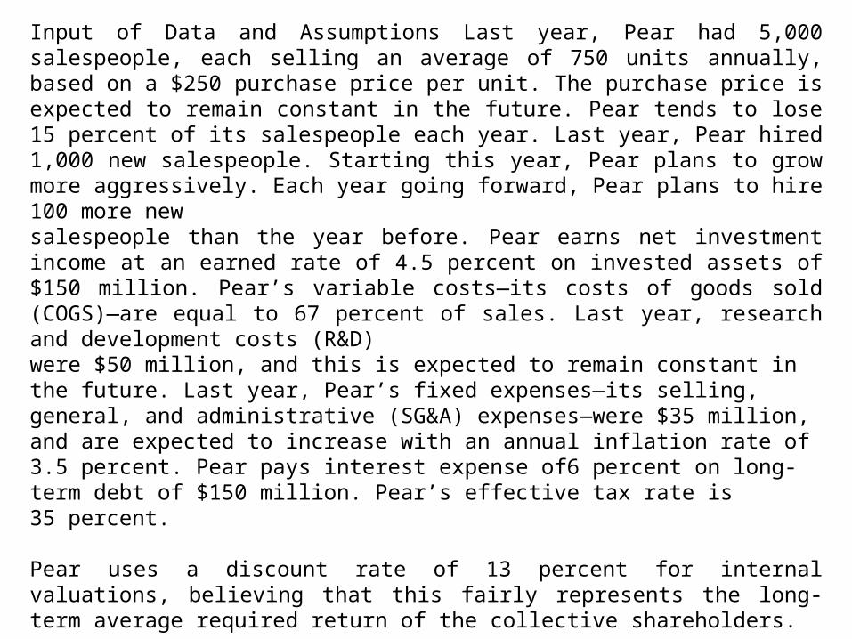
Input of Data and Assumptions Last year, Pear had 5,000 salespeople, each selling an average of 750 units annually, based on a $250 purchase price per unit. The purchase price is expected to remain constant in the future. Pear tends to lose 15 percent of its salespeople each year. Last year, Pear hired 1,000 new salespeople. Starting this year, Pear plans to grow more aggressively. Each year going forward, Pear plans to hire 100 more newsalespeople than the year before. Pear earns net investment income at an earned rate of 4.5 percent on invested assets of $150 million. Pear’s variable costs—its costs of goods sold (COGS)—are equal to 67 percent of sales. Last year, research and development costs (R&D)were $50 million, and this is expected to remain constant in the future. Last year, Pear’s fixed expenses—its selling, general, and administrative (SG&A) expenses—were $35 million, and are expected to increase with an annual inflation rate of 3.5 percent. Pear pays interest expense of6 percent on long-term debt of $150 million. Pear’s effective tax rate is35 percent.

Pear uses a discount rate of 13 percent for internal valuations, believing that this fairly represents the long-term average required return of the collective shareholders.

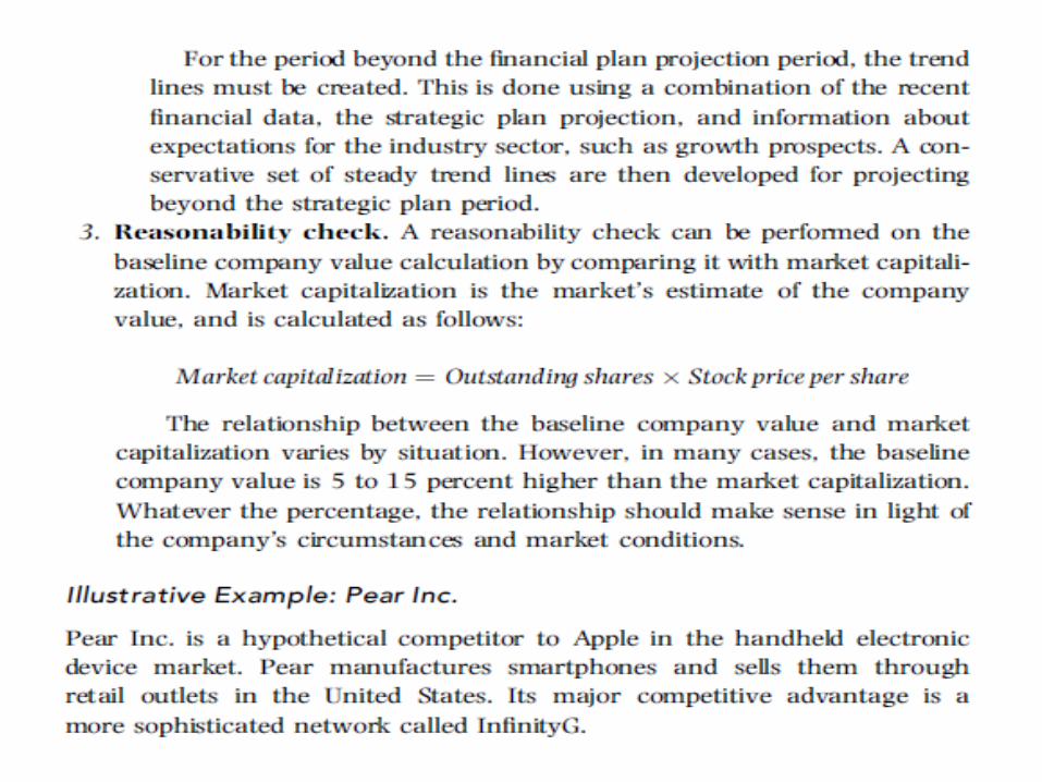
Pear has 200 million shares outstanding. The current stock price is $8.75per share, resulting in a market capitalization of $1.75 billion.

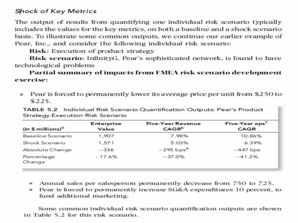
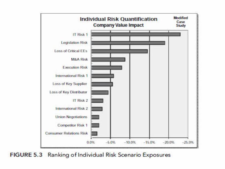
At this point, all we have done is individually quantify the risk scenarios. We have not yet calculated any interactivity between risk scenarios, which is part of the next risk quantification activity—calculating enterprise risk exposure.Yet, this is still quite valuable information, and it immediately spurs management action. Once management sees the potential impact to company value, they take actions. These actions are further informed by the attribution information discussed next. In addition, several case studies illustrating this point are presented later.

Attribution of ShocksBy itself, calculating the shock impact of individual risk scenarios on company value is powerful information. It shows management the connection of risk to value, focusing priorities and clarifying a business case for decision making involving mitigation. However, specific mitigation actions are further informed by calculating an attribution of the individualrisk scenario shocks to company value. This reveals how much each component risk driver contributes to the overall shock to company value. For example, assume a risk scenario includes two component drivers—one being a reduction in revenues and another being an increase in variable expenses. The attribution would show how much of the total value shock was separately caused by each component driver: the value shock from therevenue decrease and, separately, the value shock from the variable expense increase.

There are several ways to calculate attribution for each component driver. Two examples of methodologies are as follows:

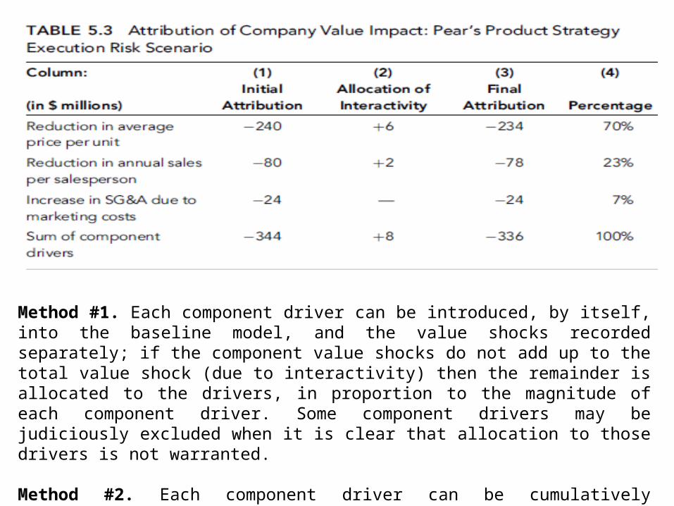
Method #1. Each component driver can be introduced, by itself, into the baseline model, and the value shocks recorded separately; if the component value shocks do not add up to the total value shock (due to interactivity) then the remainder is allocated to the drivers, in proportion to the magnitude of each component driver. Some component drivers may be judiciously excluded when it is clear that allocation to those drivers is not warranted.

Method #2. Each component driver can be cumulatively introduced into the model, one at a time, in some chosen order, with each marginal value shock attributed to the newly introduced driver.