Risk Measurement for Financial Institutions

Dr. Graeme WestFinancial Modelling Agency

www.finmod.co.zagraeme@finmod.co.za

July 13, 2006

Contents

1 Risk types and their measurement 3

1.1 Market Risk . . . . . . . . . . . . . . . . . . . . . . . . . . . . . . . . . . . . . . . . . . 3

1.2 Credit Risk . . . . . . . . . . . . . . . . . . . . . . . . . . . . . . . . . . . . . . . . . . 3

1.3 Market imperfections . . . . . . . . . . . . . . . . . . . . . . . . . . . . . . . . . . . . . 4

1.4 Liquidity risk . . . . . . . . . . . . . . . . . . . . . . . . . . . . . . . . . . . . . . . . . 5

1.5 Operational risk . . . . . . . . . . . . . . . . . . . . . . . . . . . . . . . . . . . . . . . 6

1.6 Legal risk . . . . . . . . . . . . . . . . . . . . . . . . . . . . . . . . . . . . . . . . . . . 6

2 Infamous risk management disasters 7

2.1 Wall street crash of 1987 . . . . . . . . . . . . . . . . . . . . . . . . . . . . . . . . . . . 7

2.2 Metallgesellschaft . . . . . . . . . . . . . . . . . . . . . . . . . . . . . . . . . . . . . . . 7

2.3 Kidder Peabody . . . . . . . . . . . . . . . . . . . . . . . . . . . . . . . . . . . . . . . 8

2.4 Barings . . . . . . . . . . . . . . . . . . . . . . . . . . . . . . . . . . . . . . . . . . . . 8

2.5 US S&L Industry . . . . . . . . . . . . . . . . . . . . . . . . . . . . . . . . . . . . . . . 9

2.6 Orange County . . . . . . . . . . . . . . . . . . . . . . . . . . . . . . . . . . . . . . . . 9

2.7 LTCM . . . . . . . . . . . . . . . . . . . . . . . . . . . . . . . . . . . . . . . . . . . . . 9

2.8 Allied Irish Bank . . . . . . . . . . . . . . . . . . . . . . . . . . . . . . . . . . . . . . . 10

2.9 National Australia Bank . . . . . . . . . . . . . . . . . . . . . . . . . . . . . . . . . . . 10

3 Value at Risk 12

3.1 RiskMetrics© . . . . . . . . . . . . . . . . . . . . . . . . . . . . . . . . . . . . . . . . . 14

3.2 Classical historical simulation . . . . . . . . . . . . . . . . . . . . . . . . . . . . . . . . 20

3.3 Historical simulation with volatility adjusting . . . . . . . . . . . . . . . . . . . . . . . 20

3.4 Monte Carlo method . . . . . . . . . . . . . . . . . . . . . . . . . . . . . . . . . . . . . 22

3.5 Summary . . . . . . . . . . . . . . . . . . . . . . . . . . . . . . . . . . . . . . . . . . . 25

4 Stress testing and Sensitivities 27

4.1 VaR can be an inadequate measure of risk . . . . . . . . . . . . . . . . . . . . . . . . . 27

4.2 Stress Testing . . . . . . . . . . . . . . . . . . . . . . . . . . . . . . . . . . . . . . . . . 27

4.3 Other risk measures and their uses . . . . . . . . . . . . . . . . . . . . . . . . . . . . . 28

1

4.4 Calculating analytic Greeks . . . . . . . . . . . . . . . . . . . . . . . . . . . . . . . . . 30

4.4.1 Interest rate instruments . . . . . . . . . . . . . . . . . . . . . . . . . . . . . . . 30

4.4.2 Equity Forwards . . . . . . . . . . . . . . . . . . . . . . . . . . . . . . . . . . . 31

4.5 Numeric greeks for equity instruments . . . . . . . . . . . . . . . . . . . . . . . . . . . 31

4.5.1 What is a numeric sensitivity? . . . . . . . . . . . . . . . . . . . . . . . . . . . 31

4.5.2 Algorithms for calculating numeric sensitivities . . . . . . . . . . . . . . . . . . 33

4.5.3 Taylor series . . . . . . . . . . . . . . . . . . . . . . . . . . . . . . . . . . . . . 34

5 The regulatory environment 35

5.1 Backtesting . . . . . . . . . . . . . . . . . . . . . . . . . . . . . . . . . . . . . . . . . . 35

5.2 Other requirements for internal model approval . . . . . . . . . . . . . . . . . . . . . . 38

5.3 Credit and operational risk measures . . . . . . . . . . . . . . . . . . . . . . . . . . . . 39

5.3.1 Basel I . . . . . . . . . . . . . . . . . . . . . . . . . . . . . . . . . . . . . . . . . 39

5.3.2 Basel II . . . . . . . . . . . . . . . . . . . . . . . . . . . . . . . . . . . . . . . . 41

6 Coherent risk measures 45

6.1 VaR cannot be used for calculating diversification . . . . . . . . . . . . . . . . . . . . . 45

6.2 Risk measures and coherence . . . . . . . . . . . . . . . . . . . . . . . . . . . . . . . . 45

6.3 Measuring diversification . . . . . . . . . . . . . . . . . . . . . . . . . . . . . . . . . . . 47

6.4 Coherent capital allocation . . . . . . . . . . . . . . . . . . . . . . . . . . . . . . . . . 47

6.5 Greek Attribution . . . . . . . . . . . . . . . . . . . . . . . . . . . . . . . . . . . . . . 49

2

Chapter 1

Risk types and their measurement

There are various types of risk. A common classification of risks is based on the source of theunderlying uncertainty.

1.1 Market Risk

By market risk, we mean the potential for unexpected changes in value of a position resulting fromchanges in market prices, which results in uncertainty of future earnings resulting from changes inmarket conditions, (e.g., prices of assets, interest rates).

These pricing parameters include security prices, interest rates, volatility, and correlation and inter-relationships.

Over the last few years measures of market risk have evolved to become synonymous with stresstesting, measurement of sensitivities, and VaR measurement.

1.2 Credit Risk

Credit risk is a significant element of the galaxy of risks facing the derivatives dealer and the derivativesend-user. There are different grades of credit risk. The most obvious one is the risk of default. Defaultmeans that the counterparty to which one is exposed will cease to make payments on obligations intowhich it has entered because it is unable to make such payments.

This is the worst case credit event that can take place. From this point of view, credit risk has threemain components:

• Probability of default - probability that a counterparty will not be able to meet its contractualobligations

• Recovery Rate - percentage of the claim we will recover if the counterparty defaults

• Credit Exposure - this related to the exposure we have if the counterparty defaults

But this view is very naive. An intermediate credit risk occurs when the counterparty’s creditworthi-ness is downgraded by the credit agencies causing the value of obligations it has issued to decline invalue. One can see immediately that market risk and credit risk interact in that the contracts intowhich we enter with counterparties will fluctuate in value with changes in market prices, thus affect-ing the size of our credit exposure. Note also that we are only exposed to credit risk on contracts in

3

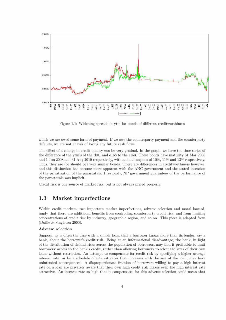
Figure 1.1: Widening spreads in ytm for bonds of different creditworthiness

which we are owed some form of payment. If we owe the counterparty payment and the counterpartydefaults, we are not at risk of losing any future cash flows.

The effect of a change in credit quality can be very gradual. In the graph, we have the time series ofthe difference of the ytm’s of the tk01 and e168 to the r153. These bonds have maturity 31 Mar 2008and 1 Jun 2008 and 31 Aug 2010 respectively, with annual coupons of 10%, 11% and 13% respectively.Thus, they are (or should be) very similar bonds. There are differences in creditworthiness however,and this distinction has become more apparent with the ANC government and the stated intentionof the privatisation of the parastatals. Previously, NP government guarantees of the performance ofthe parastatals was implicit.

Credit risk is one source of market risk, but is not always priced properly.

1.3 Market imperfections

Within credit markets, two important market imperfections, adverse selection and moral hazard,imply that there are additional benefits from controlling counterparty credit risk, and from limitingconcentrations of credit risk by industry, geographic region, and so on. This piece is adapted from(Duffie & Singleton 2000).

Adverse selection

Suppose, as is often the case with a simple loan, that a borrower knows more than its lender, say abank, about the borrower’s credit risk. Being at an informational disadvantage, the bank, in lightof the distribution of default risks across the population of borrowers, may find it profitable to limitborrowers’ access to the bank’s credit, rather than allowing borrowers to select the sizes of their ownloans without restriction. An attempt to compensate for credit risk by specifying a higher averageinterest rate, or by a schedule of interest rates that increases with the size of the loan, may haveunintended consequences. A disproportionate fraction of borrowers willing to pay a high interestrate on a loan are privately aware that their own high credit risk makes even the high interest rateattractive. An interest rate so high that it compensates for this adverse selection could mean that

4

almost no borrower finds a loan attractive, and that the bank would do little or no business.

It usually is more effective to limit access to credit. Even though adverse selection can still occur tosome degree, the bank can earn profits on average, depending on the distribution of default risk in thepopulation of borrowers. When a bank does have some information on the credit quality of individualborrowers (that it can legally use to set borrowing rates or access to credit) the bank can use bothprice and quantity controls to enhance the profitability of its lending operations. For example, bankstypically set interest rates according to the credit ratings of borrowers, coupled with limited access tocredit.

In the case of an over-the-counter derivative, such as a swap, an analogous asymmetry of creditinformation often exists. For example, counterparty A is typically better informed about its owncredit quality than about the credit quality of counterparty B. (Likewise B usually knows moreabout its own default risk than about the default risk of A.) By the same adverse-selection reasoningdescribed above for loans, A may wish to limit the extent of its exposure to default by B. Likewise,B does not wish its potential exposure to default by counterparty A to become large. Rather thanlimiting access to credit in terms of the notional size of the swap, or its market value (which in anycase is typically zero at inception), it makes sense to measure credit risk in terms of the probabilitydistribution of the exposure to default by the other counterparty.

Moral hazard

Within banking circles, there is a well known saying: “If you owe your bank R100,000 that you don’thave, your are in big trouble. If you owe your bank R100,000,000 that you don’t have, your bank is inbig trouble.” One of the reasons that large loans are more risky than small loans, other things beingequal, is that they provide incentives for borrowers to undertake riskier behaviour. If these big betsturn out badly (as they ultimately did in many cases) the risk takers can walk away. If the big betspay off, there are large gains.

An obvious defence against the moral hazard induced by offering large loans to risky borrowers is tolimit access to credit. The same story applies, in effect, with over-the-counter derivatives. Indeed, itmakes sense, when examining the probability distribution of credit exposure on an OTC derivative,to use measures that place special emphasis on the largest potential exposures.

1.4 Liquidity risk

Liquidity risk is reflected in the increased costs of adjusting financial positions. This may be evidencedby bid-ask spreads widening; more dramatically arbitrage-free relationships fail or the market maydisappear altogether. In extreme conditions a firm may lose its access to credit, and have an inabilityto fund its illiquid assets.

There are 2 types of liquidity risk:

• Normal or usual liquidity risk - this risk arises from dealing in markets that are less than fullyliquid in their standard day-to-day operation. This occurs in almost all financial markets but ismore severe in developing markets and. specialist OC instruments.

• Crises liquidity risk - liquidity arising because of market crises e.g. times of crisis such as 1987crash, the ERM crisis of 1992, the Russian crisis in August 1998, and the SE Asian crisis of1998, we find the market had lost its normal level of liquidity. One can only liquidate positionsby taking much larger losses.

5

1.5 Operational risk

This includes the risk of a mistake or breakdown in the trading, settlement or risk-managementoperation. These include

• trading errors

• not understanding the deal, deal mispricing

• parameter measurement errors

• back office oversight such as not exercising in the money options

• information systems failures

An important type of operational risk is management errors, neglect or incompetence which can beevidenced by

• unmonitored trading, fraud, rogue trading

• insufficient attention to developing and then testing risk management systems

• breakdown of customer relations

• regulatory and legal problems

• the insidious failure to quantify the risk appetite.

1.6 Legal risk

Legal risk is the risk of loss arising from uncertainty about the enforceability of contracts.

Its includes risks from:

• Arguments over insufficient documentation

• Alleged breach of conditions

• Enforceability of contract provisions - regards netting, collateral or third-party guarantees indefault of bankruptcy

Legal risk has been a particular issue with derivative contracts. Many banks found their swapscontracts with London Boroughs of Hammersmith and Fulham voided when the courts of Englandupheld the argument that the borough management did not have the legal authority to deal in swaps.

6

Chapter 2

Infamous risk managementdisasters

In all the cases we discuss the institution was exposed to risks, supposedly without managementbeing aware of them. But in many cases senior management were aware of the weaknesses in theirrisk-control systems, (or should have been) but failed to act. And very often the risks would havebeen picked up even with the simplest VaR implementation.

2.1 Wall street crash of 1987

When the portfolio insurance policy comprises a protective put position, no adjustment is requiredonce the strategy is in place. However, when insurance is effected through equivalent dynamic hedgingin index futures and risk free bills, it destabilises markets by supporting downward trends. This isbecause dynamic hedging involves selling index futures when stock prices fall. This causes the pricesof index futures to fall below their theoretical cost-of-carry value. Then index arbitrageurs step into close the gap between the futures and the underlying stock market by buying futures and sellingstocks through a sell program trade.

2.2 Metallgesellschaft

Metallgesellschaft is a huge German industrial conglomerate dealing in energy products. From 1990to 1993 they sold long-term forward contracts supplying oil products (the equivalent of 180 millionbarrels of oil) to their consumers. In order to hedge the position, they went long a like number of oilfutures.

However, futures are short term contracts. As each future expired, they rolled it over to the nextexpiry. Of course, this exposed the company to basis risk.

The price of oil decreased. Thus they made a loss on the futures position and a profit on the OTCforwards. The problem is that losses on futures lead to margin calls whereas the profits on the forwardswere still a long time from being realised. In fact, there were $1 billion margin calls on the futurespositions.

The management of Metallgesellschaft were unwilling to continue to fund the position. They firedall the dealers, closed out all the futures positions, and allowed the counterparties to the forwards towalk away.

A loss of $1.3 billion was incurred. The share price fell from 64DM to 24DM.

7

Figure 2.1: The price of oil (Dubai)

2.3 Kidder Peabody

In April 1994, Kidder announced that losses at its government bond desk would lead to a $210million charge against earnings, reversing what had been expected to be the firm’s largest quarterlyprofit in its 129-year history. The company disclosed that Joseph Jett, the head of the governmentbond desk, had manufactured $350 million in “phantom” trading profits, in what the Securities andExchange Commission later called a “merciless” exploitation of the firm’s computer system. Kidder’sinternal report on the incident concluded that the deception went unnoticed for two years due to “laxsupervision”. Mr. Jett, who denied that his actions were unknown to his superiors, was found guiltyof recordkeeping violations by an administrative judge.

2.4 Barings

This is probably the most famous banking disaster of all. Early in 1995, the futures desk of Baring’sin Singapore was controlled by Nic Leeson, a 28 year old trader.

He had long and unauthorised speculative futures positions on the Nikkei.

However, the Nikkei fell significantly. This was in no small part due to the Kobe earthquake of 17January. He was faced with huge margin calls, which for a while he funded by taking option premia.However, eventually there was no more funds, and he absconded on 23 February 1995. The bankofficially failed 26 February 1995, with a loss of $1 billion.

Leeson was sentenced to 6 and a half years in prison. The bank was sold for 1 pound to ING.

The reasons for failure: outright operational failure, tardiness of exchanges, tardiness of the Bank ofEngland.

In a survey of 1997 (Paul-Choudhury 1997):

• 75% of risk managers believed that their organisation could not suffer a Barings-type disaster.

8

Figure 2.2: The Nikkei index

• 75% of traders believed that their organisation could suffer a Barings-type disaster.

• 85% of traders believed that they could hide trades from their risk manager.

2.5 US S&L Industry

In the 1980s, Savings-and-Loan institutions were making long term loans in housing and property at afixed rate, and taking short term deposits such as mortgage payments. In the face of market volatilityand changes in the shape of the interest rate term struture, the US Congress made the mistake ofderegulating the industry. This allows moral hazard.

One consequence of this deregulation was that savings-and-loan institutions has access to extensivecredit through deposit insurance, while at the same time there was no real enforcement of limits onthe riskiness of savings-and-loans investments. This encouraged some savings-and-loans owners totake on highly levered and risky portfolios of long-term loans, mortgage-backed securities, and otherrisky assets. Many went insolvent.

2.6 Orange County

The investment pool was invested in highly leveraged investments. The dealer Bob Citron insistedthat MtM was irrelevant because a hold to maturity strategy was followed. This nonsense was believedfor some time, but the eventual outcome was bankruptcy.

2.7 LTCM

Long Term Capital Management failed spectacularly in 1998. This was a very exclusive hedge fundwhose partners included Myron Scholes, Robert Merton and John Meriwether. Their basic play, all

9

over the world, was on credit spreads narrowing - thus, they were typically long credit risky bondsand short credit-safe bonds.

What were the reasons?

• Widening credit spreads and liquidity squeeze after the Russian default of 1998 - subsequenttalk of a market in liquidity options by Scholes, amongst others.

• Very large leverage, which increased as the trouble increased, and as liquidity dried up. In otherwords, not enough long term capital.

• Excessive reliance on VaR without performing stress testing. They were caught out as a newparadigm was emerging: as VaR inputs are always historical, none of what was happening wasan ‘input’ to the VaR model.

• Model risk - too many complex plays. Infatuation with sexy deals, which were retained as theportfolio was reduced. This reduced the liquidity even further.

LTCM was bailed out under rather suspicious circumstances by a consortium of creditors organised byAlan Greenspan of the Federal Reserve Bank. The exact conditions and motives for this are still notknown - involvement by the legislators increases moral hazard going forward. It was argued that failureof LTCM could destabilise international capital markets. See (Kolman April 1999), (The FinancialEconomists Roundtable October 6, 1999), and the standard book on the subject, (Lowenstein 2000).

2.8 Allied Irish Bank

More recently, Allied Irish Banks PLC disclosed in February that a rogue trader accumulated almost$700 million in losses over a five-year period. The losses, incurred at its U.S. foreign exchangeoperation Allfirst, caused the company to reduce its 2001 net income by over $260 million (about38%). The Wall Street Journal claimed that Allfirst had a 25-year-old junior employee monitoringcurrency trading risk, an assertion that the bank denied. Bank officials believe that John Rusnakavoided the company’s internal checks by contracting out administration to banks that were complicitin the fraud.

2.9 National Australia Bank

The NAB options team made a loss in October 2003, right around the time they were expecting theirperformance bonuses, and rather than jeopardise them they tried to push the loss forward and waitfor an opportunity to trade out of it - then decided to bet on the Australian dollar dropping. Withthe Australian dollar charging ahead in late 2003, they were left with a $180m loss within weeks.

One of the dealers was open with the press. His most serious claim was that the bank’s risk-management department had been signing off on the losses for months. “We were already overthe limits for a number of months and the bank knew about it... It has been going on and off for ayear and consistently every day since October. It was signed off every day by the risk-managementpeople.”

This is a direct contradiction of the bank’s claims that the $180 million loss was the result of unau-thorised trades that had been hidden from senior management.

A former options trader wrote: “I can tell you that NAB have been doing dodgy trading stuff formuch longer than a few months. The global FX options market has been waiting for them to blowup for years. No-one is surprised by this at all, except the fact that it took so long.”

The risk management situation at NAB seemed very poor. Chris Lewis was the senior KPMG auditorwho had headed a due diligence team to advice whether the bank should buy Homeside in Florida;

10

this advise was in the affirmative. As auditor he also signed the 2000 accounts and claimed they were“free of material mis-statement”, when in fact the bank was about to lose $3.6 billion from mortgageservicing risk at Homeside, which wasn’t even mentioned in the annual report.

Lewis was hired as the head of risk soon afterwards! It is clearly a conflict to have auditors who spendyears convincing themselves everything is okay and then go and take over the reigns of internal auditat the same client, as there is a lack of fresh perspective. Not to mention that his competency was inquestion.

11

Chapter 3

Value at Risk

We will focus for the remainder of this course on measuring market risks. It is only measurementof this type of risk, that has evolved to a state of near-finality, from a quantitative point of view.The standard ways of measuring market risks is via VaR or a relative thereof, stress testing, andsensitivities.

VaR was the first risk management tool developed that took into account portfolio and diversificationeffects.

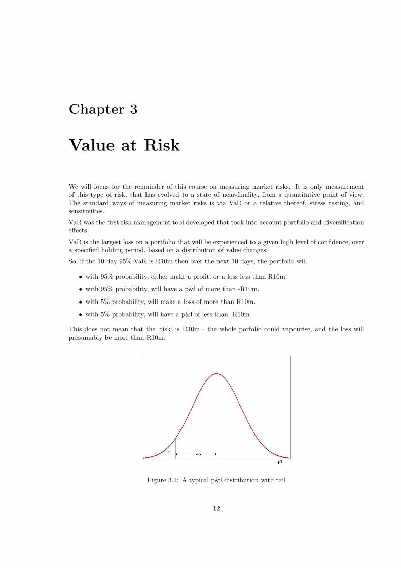
VaR is the largest loss on a portfolio that will be experienced to a given high level of confidence, overa specified holding period, based on a distribution of value changes.

So, if the 10 day 95% VaR is R10m then over the next 10 days, the portfolio will

• with 95% probability, either make a profit, or a loss less than R10m.

• with 95% probability, will have a p&l of more than -R10m.

• with 5% probability, will make a loss of more than R10m.

• with 5% probability, will have a p&l of less than -R10m.

This does not mean that the ‘risk’ is R10m - the whole porfolio could vapourise, and the loss willpresumably be more than R10m.

Figure 3.1: A typical p&l distribution with tail

12

The term 10 days above is known as the ‘holding period’.

The term 95% is known as the ‘confidence level’.

Thus, a formal definition:

Definition 1 The N -day VaR is x at the α confidence level means that, according to a distributionof value changes, with probability α, the total p&l over the next N days will be −x or more.

Are the following consistent?

• 1 day 95% VaR of R10m

• 1 day 99% VaR of R5m

Certainly not. As our confidence increases the VaR number must increase. So, we might have

• 1 day 95% VaR of R10m

• 1 day 99% VaR of R20m

Are the following consistent?

• 1 day 95% VaR of R10m

• 1 day 99% VaR of R20m

• 10 day 99% VaR of R20m

Certainly not. More likely we would have:

• 10 day 99% VaR of R40m, say.

So, the following may very well be consistent:

• 1 day 95% VaR of R10m

• 1 day 99% VaR of R20m

• 10 day 99% VaR of R40m

Changing the holding period or the confidence level changes the reported VaR, but not the reality.

What are the factors driving the VaR of a position?

• size of positions - should be linear in size. But in extreme cases the size of the position affectsthe liquidity.

• direction of positions - not linear in direction eg. a call.

• riskiness of the positions - more speculative positions and/or more volatility should contributeto an increase in VaR.

• the combination of positions - correlation between positions.

’Distribution of value changes’ - distribution needs to be determined, either explicitly or implicitly,and sampled. Current VaR possibilities:

13

• The Variance-Covariance approach, in other words the classic RiskMetrics© approach, or avariation thereof.

• Various historical simulation approaches - ‘history repeats itself’.

• Monte Carlo simulation.

The choice of VaR method can be a function of the nature of the portfolio. For fixed income and equity,a variance-covariance approach is probably adequate. For plain vanilla options a simple enhancementof VCV such as the delta-gamma approach is often claimed to be suitable (the author disagrees), butif there are more exotic options, a more advanced full revaluation method is required such as historicalor Monte Carlo.

The fundamental problem we are faced with is how to aggregate risks of various positions. Theycannot just be added, because of possible interactions (correlations) between the risks.

In making the decision of which method to use, there is a tradeoff between computational time spentand the ‘accuracy’ of the model. It should be noted in this regard that traders will attempt to gamethe model if their limits or remuneration is a function of the VaR number and there are perceivedor actual limitations to the VaR calculation. Thus (as already mentioned) limits on VaR need to besupplemented by limits on notionals, on the sensitivities, and by stress and scenario testing.

3.1 RiskMetrics©

In the following examples we compute VaR using standard deviations and correlations of financialreturns, under the assumption that these returns are normally distributed. In most markets thestatistical information is provided by RiskMetrics, but in South Africa, for example, the data isprovided a day late. This is unsatisfactory for immediate risk management. Thus the institutionshould have their own databases of RiskMetrics type data.

The RiskMetrics assumption is that standardised returns are normally distributed given the value ofthis standard deviation. This is of course the fundamental Geometric Brownian Motion model.

α% VaR is derived via −zα times the standard deviation of returns, which is given by σ√250

, whereσ is the annualised volatility of returns. Here z· is the inverse of the cumulative normal distribution,so, for example, if α = 95% then −z0.95 = −1.645. Thus, a ‘bad’ outcome, for a portfolio which ispositive valued, would be a negative stock return of −zα

σ√250

, and the VaR is

V

(1− exp

(−zα

σ√250

))(3.1)

If the portfolio is negative valued, the bad outcome would be a positive stock return of zασ√250

, andso the VaR is

V

(1− exp

(zα

σ√250

))(3.2)

Note here we have two negatives, giving us a positive VaR value.

We will call this approach the ‘RiskMetrics full precision’ method. For another possibility, note thatby Taylor series 1−ex ≈ −x ≈ e−x−1. Hence, for either a long or short position, VaR is approximatelygiven by

|V |zασ√250

(3.3)

We will call this the ‘standard RiskMetrics simplification’. Indeed, when reading (J.P.Morgan &Reuters December 18, 1996) it is very problematic to know at any stage which method is being referredto. Unfortunately, the standard simplification method does not have much theoretical motivation:prices are not normally distributed under any model - it is returns that are typically modelled asbeing normal.

14

Example 1 You hold 2,000,000 shares of SAB. Currently the share is trading at 70.90 and thevolatility of the return of SAB, measured historically, is 24.31%.

What is your 95% VaR over a 1-day horizon on 23-Jan-04?

Your exposure is equal to the market value of the position in ZAR. The market value of the positionis 2, 000, 000 · 70.90 = 141, 800, 000.

The VaR of the position is 2, 000, 000 · 70.90 ·(1− exp

(−z0.95

24.31%√250

))= 3, 540, 616.

Now suppose we have a portfolio. Here the covolatility matrix Σ is measured in returns. Then σ(R)is the volatility of the return of the portfolio, and is found as σ(R) =

√w′Σw as in classical portfolio

theory. Here wi are the proportional value weights, with∑n

i=1 wi = 1. So VaR can be measureddirectly. The assumption is again made that the return R is normally distributed, and the formulaefor VaR are as before.

Example 2 You hold 2,000,000 shares of SAB and 500000 shares of SOL. SOL is trading at 105.20with a volatility of 32.10%. The correlation in returns is 4.14%. What is your 95% VaR over a 1-dayhorizon on 23-Jan-04?

This time, the MtM is 2, 000, 000 · 70.90 + 500000 · 105.20 = 194, 400, 000.

The daily standard deviation in returns are σ1 = 1.54% and σ2 = 2.03%. The value weights arew1 = 72.94% and w2 = 27.06%. The correlation in returns is ρ = 4.14%. Thus, using the portfoliotheory formula for the standard deviation of the returns of a portfolio,

σ(R) =√

w21σ

21 + 2w1w2ρσ1σ2 + w2

2σ22 (3.4)

which is equal to 1.27% in this case. The VaR calculation proceeds as before, yielding a VaR of4,015,381.

This is a good opportunity to introduce the concept of undiversified VaR. We calculate the VaRfor each instrument on a stand-alone basis: VaR1 = 3, 540, 616 and VaR2 = 1, 727, 495, for a totalundiversified VaR of 5,268,111. The fact that the VaR of the portfolio is actually 4,015,381 is anillustration of portfolio benefits.

RiskMetrics provides users with 1.645σ1, 1.645σ2, and ρ. One has to take care of the factor 1.645:whether to leave it in or divide it out, according to the required application. As has been indicated,this information is certainly provided in the South African environment, but it is a day late. It is notdifficult to calculate these numbers oneself, using the prescribed methodology. The EWMA methodwith λ = 0.94 is the method prescribed by RiskMetrics for the volatility and correlation calculations.

If we make the standard RiskMetrics simplification, a neat simplifying trick is possible. Suppose σ(R)and Σ are daily measures. Then

VaR = |V |zασ(R) =√

V 2zα

√w′Σw = zα

√W ′ΣW (3.5)

where Wi = wiV is the value of the ith component.

Calculating VaR on a portfolio of cash flows usually involves more steps than the basic ones outlinedin the examples above. Even before calculating VaR, you need to estimate to which risk factors aparticular portfolio is exposed. The RiskMetrics methodology for doing this is to decompose financialinstruments into their basic cash flow components. We use a simple example - a bond - to demonstratehow to compute VaR. See (J.P.Morgan & Reuters December 18, 1996, §1.2.1).

Example 3 Suppose on 25-Jun-03 we are long a r150 bond. This expires 28-Feb-05, with a 12.00%coupon paid, with coupon dates 28-Feb and 31-Aug. How do we calculate VaR using the standardRiskMetrics simplification?

15

The first step is to map the cash flows onto standardised time vertices, which are 1m, 3m, 6m, 1y,2y, 3y, 4y, 5y, 7y, 9y, 10y, 15y, 20y and 30y (J.P.Morgan & Reuters December 18, 1996, §6.2). Wewill suppose we have the volatilities and correlations of the return of the zero coupon bond for all ofthese time vertices.

The actual cash flows are converted to RiskMetrics cash flows by mapping (redistributing) them ontothe RiskMetrics vertices. The purpose of the mapping is to standardize the cash flow intervals of theinstrument such that we can use the volatilities and correlations of the prices of zero coupon bondsthat are routinely computed for the given vertices in the RiskMetrics data sets. (It would be impossibleto provide volatility and correlation estimates on every possible maturity so RiskMetrics provides amapping methodology which distributes cash flows to a workable set of standard maturities).

The RiskMetrics methodology (J.P.Morgan & Reuters December 18, 1996, Chapter 6) for mappingthese cash flows is not completely trivial, but is completely consistent. We linearly interpolate the riskfree rates at the nodes to risk free rates at the actual cash flow dates. Likewise we linearly interpolatethe price volatilities at the nodes to price volatilities at the actual cash flow dates.

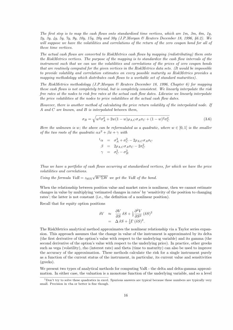
However, there is another method of calculating the price return volatility of the interpolated node. IfA and C are known, and B is interpolated between them,

σB =√

w2σ2A + 2w(1− w)ρA,CσAσC + (1− w)2σ2

C (3.6)

Here the unknown is w; the above can be reformulated as a quadratic, where w ∈ [0, 1] is the smallerof the two roots of the quadratic αx2 + βx + γ with

1α = σ2A + σ2

C − 2ρA,CσAσC

β = 2ρA,CσAσC − 2σ2C

γ = σ2C − σ2

B

Thus we have a portfolio of cash flows occurring at standardised vertices, for which we have the pricevolatilities and correlations.

Using the formula VaR = z95%

√W ′ΣW we get the VaR of the bond.

When the relationship between position value and market rates is nonlinear, then we cannot estimatechanges in value by multiplying ‘estimated changes in rates’ by ‘sensitivity of the position to changingrates’; the latter is not constant (i.e., the definition of a nonlinear position).

Recall that for equity option positions

δV ≈ ∂V

∂SδS + 1

2

∂2V

∂S2(δS)2

= ∆ δS + 12Γ (δS)2.

The RiskMetrics analytical method approximates the nonlinear relationship via a Taylor series expan-sion. This approach assumes that the change in value of the instrument is approximated by its delta(the first derivative of the option’s value with respect to the underlying variable) and its gamma (thesecond derivative of the option’s value with respect to the underlying price). In practice, other greekssuch as vega (volatility), rho (interest rate) and theta (time to maturity) can also be used to improvethe accuracy of the approximation. These methods calculate the risk for a single instrument purelyas a function of the current status of the instrument, in particular, its current value and sensitivities(greeks).

We present two types of analytical methods for computing VaR - the delta and delta-gamma approxi-mation. In either case, the valuation is a monotone function of the underlying variable, and so a level

1Don’t try to solve these quadratics in excel. Spurious answers are typical because these numbers are typically verysmall. Precision in vba or better is fine though.

16

Figure 3.2: The RiskMetrics method for cash flows (for example, coupon bonds)17

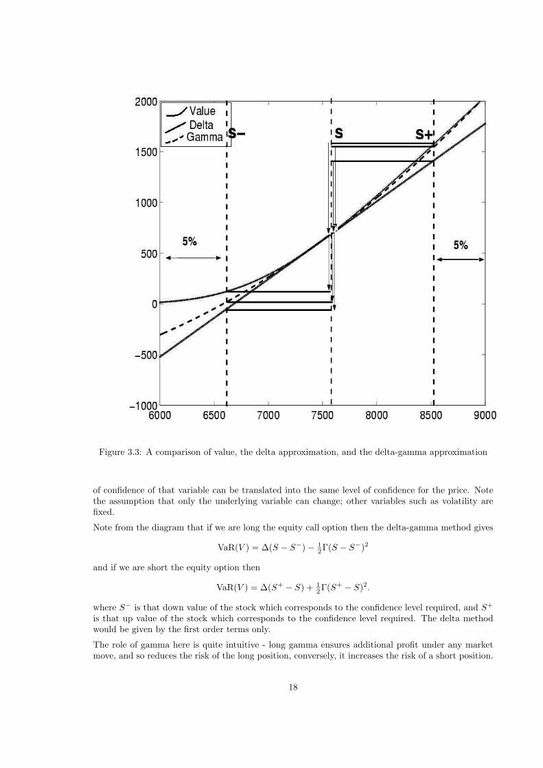
Figure 3.3: A comparison of value, the delta approximation, and the delta-gamma approximation

of confidence of that variable can be translated into the same level of confidence for the price. Notethe assumption that only the underlying variable can change; other variables such as volatility arefixed.

Note from the diagram that if we are long the equity call option then the delta-gamma method gives

VaR(V ) = ∆(S − S−)− 12Γ(S − S−)2

and if we are short the equity option then

VaR(V ) = ∆(S+ − S) + 12Γ(S+ − S)2.

where S− is that down value of the stock which corresponds to the confidence level required, and S+

is that up value of the stock which corresponds to the confidence level required. The delta methodwould be given by the first order terms only.

The role of gamma here is quite intuitive - long gamma ensures additional profit under any marketmove, and so reduces the risk of the long position, conversely, it increases the risk of a short position.

18

Because of the sign differences in whether we are long or short, care needs to be taken with aggregationusing this approach. Furthermore, this approach ignores the fact that there are other variables whichimpact the value of the position, such as the volatility in the case of an equity option, which in realityneeds to be estimated and measured frequently. Since there is a correlation between price changesand changes in volatility, this missing factor can be significant.

Furthermore, for these methods to have any meaning at all, the price of the derivative must be amonotone function of the price of the underlying.2

Example 4 Let us consider an OTC European call option on the ALSI40, expiry 17-Mar-05, strike10,000, with the current valuation date being 15-Jan-04. The RiskMetrics method will focus on pricerisk exclusively and therefore ignore the risk associated with volatility (vega), interest rate (rho) andtime decay (theta risk).

The spot of the ALSI40 is 10,048, and the dividend yield for the term of the option is estimatedas 3.00%. The risk free rate for the term of the option is 8.40% and the SAFEX volatility for theterm is 20.50%. As mentioned, we will assume that these values do not change, and we will use theSAFEX volatility without any considerations for the skew, and allowing for this blend of exchangetraded models and otc models.

The value of the position is 1,185.41, the delta is 0.638973, and the gamma 0.000158.

The daily volatility σ of the ALSI40 is 1.30%. Thus S− = Se−1.645σ = 9, 835.98, and S+ = Se1.645σ =10, 264.59. Hence, with the delta method, if we are long then

VaR(V ) = ∆(S − S−) = 135.47

and if we are short thenVaR(V ) = ∆(S+ − S) = 138.39

and with the delta-gamma method, if we are long then

VaR(V ) = ∆(S − S−)− 12Γ(S − S−)2 = 131.91

and if we are short then

VaR(V ) = ∆(S+ − S) + 12Γ(S+ − S)2 = 142.11.

The delta approximation is reasonably accurate when the spot does not change significantly, but lessso in the more extreme cases. This is because the delta is a linear approximation of a non linearrelationship between the value of the spot and the price of the option. We may be able to improvethis approximation by including the gamma term, which accounts for nonlinear (i.e. squared returns)effects of changes in the spot.

Note that in this example, how incorporating gamma changes VaR relative to the delta-only approx-imation.

The main attraction of such a method is its simplicity, however, this is also the problem. This approachignores other effects such as interest rate and volatility exposure, and fits a normal distribution todata which is known not to be normally distributed. As such it will underestimate the frequencyof large moves and should underestimate the ‘true VaR’. This method is really only suitable for thesimplest portfolios.

Despite the number of possibly tenuous assumptions, RiskMetrics performs satisfactorily well in back-testing. (Pafka & Kondor 2001) claim that this is an artifact of the choice of the risk measure: firstlythat the forecasting horizon is one day, and secondly that the significance level is 95%. The first factorallows even fairly crude volatility models to perform well, and secondly the fact that the significancelevel is not too high means that the fat tail effect is not too severe.

2For example, how would one use methods like this to do calculations involving barrier options, which have tradedin the South African market?

19

For more complicated portfolios - ones with several instruments, including options, the RiskMetricapproach involves moment matching. For this, see (Zangari 1996), (Mina & Ulmer April 1999),(Pichler & Selitsch 2000) and (Hull 2002, Chapter 16).

3.2 Classical historical simulation

The historical method is a full revaluation method. The revaluation of the entire portfolio is calculatedfor each of the last N days, as if the evolution in market variables that occurred on each of those dayswas to reoccur now. Thus,

lnxi

x(t)= ln

x(i)x(i− 1)

(3.7)

or

xi = x(t) · x(i)x(i− 1)

(3.8)

would be the market factor update formula for the variable x. Here t denotes the current day, i oneof the past business days, t−N + 1 ≤ i ≤ t, and i− 1 the business day before that.

Example 5 Suppose on 22-Jan-04 we are long a r153 bond. We perform 400 historical simulationson the ytm. We then apply the bond pricing formula ie. full revaluation to the ytms so obtained toget the all in price of the bond on 28-Jan-04. This is FOUR business days after 22-Jan-04, which isthree days after the next business date.

We get from full revaluation 400 bond prices: a minimum of 1.2316, a 5th percentile of 1.2387, anaverage of 1.2440, a 95th percentile of 1.2497, and a maximum of 1.2600. Thus if we are long thebond then the 95% VaR is 0.0054 per unit, and if we are short then the 95% VaR is 0.0057 per unit.

We could also simply determine the appropriate percentile ytm and calculate the AIP there, to get thesame results. However, this does not help as soon as we start aggregation.

Example 6 Let us consider an OTC European call option on the ALSI40; expiry 20-Mar-03, strike12000, with the current valuation date being 19-Jun-02. We perform 400 historical simulations on thespot, on the risk free rate, and on the atm volatility, valuing on 20-Jun-02. We stress the dividend yieldin the reverse direction of the spot stress in such a manner that the monetary value of the dividendsis constant.

We get from full revaluation 400 option prices: a minimum of 294.59, a 5th percentile of 400.20, anaverage of 468.22, a 95th percentile of 551.17, and a maximum of 754.32. Thus if we are long theoption then the 95% VaR is 68.02, and if we are short then the 95% VaR is 82.95.

3.3 Historical simulation with volatility adjusting

This method was first proposed in (Hull & White 1998), and has become quite prevalent academically.It has not been widely implemented in the industry, although it is starting to gain some prominencein South Africa. One of the main critisms of the historical method is that the returns of the past canbe inappropriate for current market conditions. For example, if our window of N days is an almostentirely quiet period, and there is currently a very sudden spike in volatility, the historical methodwould still be using the ’quiet data’, and the new volatility regime would only be factored in gradually,one day at a time.

The Historical V@R method accurately reflects the historical probability distribution of the marketvariables, which is an attractive feature especially in markets where the normality assumption isfar from reality. However, historical V@R’s main disadvantage is that it incorporates no volatility

20

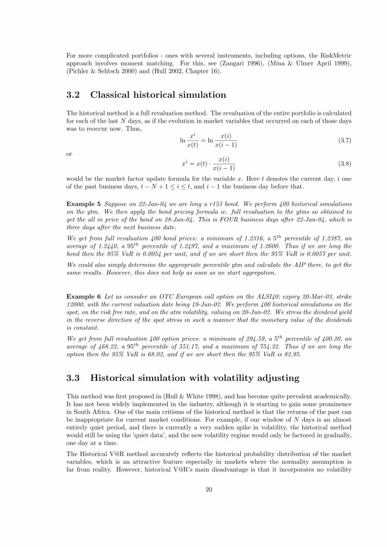
Figure 3.4: The bucketed values of the instrument in 400 experiments for historical V@R

updating, in that it assumes the distribution of returns is stationary. As we will see, the Hull-Whitemethod is a modification of the historical method that overcomes this difficulty.

If the current volatility of a market variable is 30% per day and a month ago was 15%, the returns amonth ago understate the returns we expect to see now. The Hull-White method adjusts the historicaldata on each market variable to reflect the difference between the old historical volatility of the marketvariable and its current historical volatility, so in the above example, it doubles the return that wasobserved.

The basic idea of the volatility adjusting is that we should only compare standardised variables, whichhave been standardised by dividing by their volatility. Thus

1σ(t)

lnxi

x(t)=

1σ(i− 1)

lnx(i)

x(i− 1)

or

xi = x(t) ·(

x(i)x(i− 1)

) σ(t)σ(i−1)

would be the experimental values for the factor x, indexed by the value i where t − N + 1 ≤ i ≤ t.The volatility is historical volatility, unless a reliable implied volatility is available, in which case it isimplied volatility.

An appropriate method for implied volatility updating is required. If exactly the same strategy isto be used one will need to measure and adjust by the volatility of volatility. But mathematicallyone cannot use any historical volatility calculation scheme - such as EWMA for example - as impliedvolatility does not follow a (Geometric Brownian Motion) random walk, but is mean reverting. We

21

prefer just to use straight historical for implied volatility. Thus, for implied volatility σI :

σiI = σI(t)

σI(i)σI(i− 1)

and we have three market factor update formulae:

xi = x(t) ·(

x(i)x(i− 1)

) σ(t)σ(i−1)

(3.9)

xi = x(t) ·(

x(i)x(i− 1)

) σI (t)σI (i−1)

(3.10)

σiI = σI(t)

σI(i)σI(i− 1)

(3.11)

where

• (3.9) is used where the variable x is available and implied volatility is not, so an historicalvolatility is calculated;

• (3.10) is used where the variable x is available and a reliable estimate of implied volatility is too(for example, a futures level);

• (3.11) is used on an implied volatility variable.

Very often implied volatilities are suspicious, due to being stale or illiquid, and in this case, thehistorical volatility should be preferred i.e. (3.9) should be preferred to (3.10).

Example 7 Let us consider the same OTC European call option on the ALSI40 as before: expiry20-Mar-03, strike 12,000, with the current valuation date being 19-Jun-02. We perform 400 historicalsimulations with volatility adjusting on the spot, on the risk free rate, and simple historical simulationson the atm volatility, valuing on 20-Jun-02. We stress the dividend yield as previously.

We get from full revaluation 400 option prices: a minimum of 316.66, a 5th percentile of 406.19, anaverage of 466.72, a 95th percentile of 540.30, and a maximum of 717.58. Thus if we are long theoption then the 95% VaR is 60.53, and if we are short then the 95% VaR is 73.59.

In a personal communication, Alan White says “I always liked that [the Hull-White] scheme. My viewis that the various approaches form a continuum in which different methods are used to characterizethe distributions in question. The parametric approach tries to match moments. It can evolve quicklybut fails to capture many of the details of the distributions. The historical simulation assumes thesample distribution is the population distribution. This captures the details of the distribution butevolves too slowly if the distribution is not stationary. We attempted to marry these two approaches.”

An example of a time series of p&l’s and (minus) the VaRs under various methods is as in Figure3.5. This shows, for example, how the historical method is completely inadequate: at the time of amarket crash, the VaR measure does not jump, as logically it should.

3.4 Monte Carlo method

The second alternative offered by RiskMetrics, structured Monte Carlo simulation, involves creatinga large number of possible rate scenarios and performing full revaluation of the portfolio under eachof these scenarios.

VaR is then defined as the appropriate percentile of the distribution of value changes. Due to therequired revaluations, this approach is computationally far more intensive than the analytic RiskMet-rics approach. The two RiskMetrics methods - analytic and Monte Carlo - differ not in terms of how

22

Figure 3.5: p&l’s and VaR for a long ALSI40 position

market movements are forecast (since both use the RiskMetrics volatility and correlation estimates)but in how the value of portfolios changes as a result of market movements. The analytical approachapproximates changes in value, while the structured Monte Carlo approach fully revalues portfoliosunder various scenarios.

The RiskMetrics Monte Carlo methodology consists of three major steps:

• Scenario generation, using the volatility and correlation estimates for the market factors whichdrive our portfolio, we produce a large number of future price scenarios in accordance with thelognormal models.

• For each scenario, we compute instrument (molecule) values and then portfolio values.

• We report the results of the simulation, either as a portfolio distribution or as a particular riskmeasure.

Other Monte Carlo methods may vary the first step by creating returns by (possibly quite involved)modelled distributions, using pseudo random numbers to draw a sample from the distribution. Thenext two steps are as above. The calculation of VaR then proceeds as for the historical simula-tion method. Indeed, this is very similar to the historical method except for the manner in whichexperiments are created.

The advances in RiskMetrics Monte Carlo is that one overcomes the pathologies involved with ap-proximations like the delta-gamma method.

The advances in other Monte Carlo methods over RiskMetrics Monte Carlo are in the creation of thedistributions. However, to create experiments using a Monte Carlo method is fraught with dangers.Each market variable has to be modelled according to an estimated distribution and the relationshipsbetween distributions (such as correlation or less obvious non-linear relationships, for which copulasare becoming prominent). Using the Monte Carlo approach means one is committed to the use of suchdistributions and the estimations one makes. These distributions can become inappropriate; possiblyin an insidious manner. To build and ‘keep current’ a Monte Carlo risk management system requirescontinual re-estimation, a good reserve of analytic and statistical skills, and non-automatic decisions.

23

Example 8 Suppose we hold an r153 bond on 22-Jan-04. What is the VaR?

The close was 9.10%. We estimate the annual volatility of the yield to be 12.25%. Using excel/vba, wefirst create uniformly distributed random numbers U then transform them into normally distributedrandom numbers Z by using the inverse of the cumulative normal distribution.3 We then determineour new yields: y(T +1) = y(T ) exp

(σ√250

Z). We then apply the bond pricing formula for 28-Jan-04

to get the new all in prices. We then work out the VaR, by examining averages and percentiles, in theusual way. The 95% VaR is about 6,417 (long) and 6,473 (short) per unit.

Choleski decomposition

Suppose we are interested in a portfolio with more than one security, or more generally, more thanone source of random normal noise. Let us start with the case where we have two such randomvariables. We cannot simply take two random number generators and paste them together, unless theunderlyings are independent. However, typically there will be a measured or estimated correlationbetween the two random variables, and this needs to appear in the random numbers generated.

If the two stocks were uncorrelated, we could have

r1 = a1Z1, r2 = a2Z2

With the correlation, we want the Z1 to influence r2. Thus the appropriate setup is[

r1

r2

]=

[a1,1 0a2,1 a2,2

] [Z1

Z2

]. (3.12)

or r = AZ. Thusrr′ = AZZ ′A′ (3.13)

and soΣ = AA′ (3.14)

by taking expectations. Thus, A is found as a type of lower-triangular square root matrix of theknown variance-covariance matrix Σ. The most common solution (it is not unique) is known as theCholeski decomposition. All that has been said is valid for any number of dimensions, and simplealgorithms for calculating the Choleski decomposition are available (Burden & Faires 1997, Algorithm6.6).

In the case of two variables, it is convenient to explicitly note the solution. Here

Σ =[

σ21 σ1σ2ρ

σ1σ2ρ σ22

](3.15)

and

A = 4

[σ1 0σ2ρ σ2

√1− ρ2

](3.16)

A theoretical requirement here is that the matrix Σ be positive semi-definite. The covariance matrixis in theory positive definite as long as the variables are truly different ie. we do not have the situationthat one is a linear combination of the others (so that there is some combination which gives the 0entry). If there are more assets in the matrix than number of historical data points the matrix willbe rank-deficient and so only positive semi-definite. Moreover, in practice because all parameters areestimated, and in a large matrix there will be some assets which are nearly linear combinations ofothers, and also taking into account numerical roundoff, the matrix may not be positive semi-definiteat all (Dowd 1998, §2.3.4). However, this problem has recently been completely solved (Higham 2002),by mathematically finding the (semi-definite) correlation matrix which is closest (in an appropriatenorm) to a given matrix, in particular, to our mis-estimated matrix.

3In excel this is given by the function norminv.4Note the error in (Dowd 1998, Chapter 5 §2.2).

24

Example 9 We reconsider the example in Example 2. You hold 2,000,000 shares of SAB and 500000shares of SOL. SOL is trading at 105.20 with a volatility of 32.10%. The correlation in returns is4.14%. What is your 95% VaR over a 1-day horizon on 23-Jan-04?

Using excel/vba, we first extract pairs of uniformly distributed random numbers U1, U2, then transformthem into pairs of normally distributed random numbers Z1, Z2 by using the inverse of the cumulativenormal distribution. We then apply the Choleski decomposition:

r1 =σ1√250

Z1, r2 =σ2√250

(ρZ1 +√

1− ρ2Z2) (3.17)

and determine our new prices: S1(T +1) = S1(T ) exp(r1), S2(T +1) = S2(T ) exp(r2). We then workout the portfolio MtF’s, and then work out the VaR, by examining averages and percentiles, in theusual way. The 95% VaRs are 3,979,192 and 4,058,332.

A possible example of the first few calculations is shown in Table 3.1. The calculation would typicallyuse 10,000 calculations or more.

Rnd(1) Rnd(2) Cumnorminverse(1)

Cumnorminverse(2)

Correlatedreturn(1)

Correlatedreturn(2)

MtF(1) MtF(2) New portfo-lio MtM

0.7055 0.5334 0.5404 0.0839 0.0083 0.0022 71.49 105.43 195,696,4570.5795 0.2896 0.2007 -0.555 0.0031 -0.011 71.12 104.04 194,258,3730.3019 0.7747 -0.519 0.7545 -0.008 0.0149 70.34 106.78 194,061,5640.014 0.7607 -2.197 0.7086 -0.034 0.0125 68.55 106.53 190,354,4010.8145 0.709 0.8946 0.5506 0.0138 0.0119 71.88 106.46 196,994,2250.0454 0.414 -1.692 -0.217 -0.026 -0.006 69.08 104.59 190,454,2970.8626 0.7905 1.0922 0.8081 0.0168 0.0173 72.10 107.04 197,719,253

Table 3.1: The first few experiments under a bivariate Monte Carlo run

Example 10 Consider on 22-Jan-04 a portfolio which consists of long 110,000,000 r153 and short175,000,000 tk01. The closes of these instruments are 9.10% and 9.41% respectively, with AIP for27-Jan-04 being 1.2434199 and 1.0524115 respectively, and delta -5.464 and -3.433 respectively. Thusthis is an almost delta neutral portfolio; the risks associated should be quite small.

We have σ1 = 12.25%, σ2 = 15.18%, and ρ = 91.25%.

Using excel/vba, we first extract pairs of uniformly distributed random numbers U1, U2, then transformthem into pairs of normally distributed random numbers Z1, Z2 by using the inverse of the cumulativenormal distribution. We then apply the Choleski decomposition:

r1 =σ1√250

Z1, r2 =σ2√250

(ρZ1 +√

1− ρ2Z2) (3.18)

and determine our new yields: y1(T + 1) = y1(T ) exp(r1), y2(T + 1) = y2(T ) exp(r2). We then applythe bond pricing formula to get the new all in prices. We then work out the VaR, by examiningaverages and percentiles, in the usual way. The 95% VaRs are 296,964 and 291,291.

Another very effective and computationally very efficient way around this problem is to reduce thedimensions of the problem by using principal component analysis or factor analysis. Principal compo-nent analysis is a topic on its own, and has become very prevalent in financial quantitative analysis.See (Dowd 1998, Box 3.3).

3.5 Summary

Here we summarise the essential features of the competing methods.

25

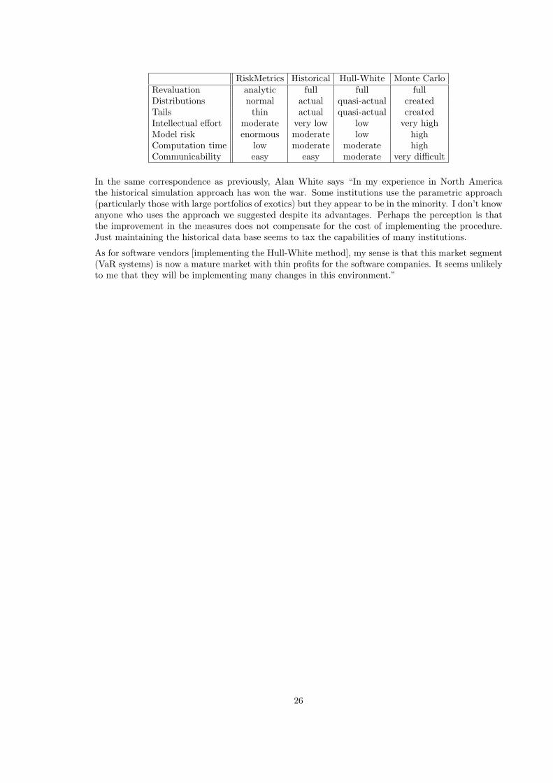
RiskMetrics Historical Hull-White Monte CarloRevaluation analytic full full fullDistributions normal actual quasi-actual createdTails thin actual quasi-actual createdIntellectual effort moderate very low low very highModel risk enormous moderate low highComputation time low moderate moderate highCommunicability easy easy moderate very difficult

In the same correspondence as previously, Alan White says “In my experience in North Americathe historical simulation approach has won the war. Some institutions use the parametric approach(particularly those with large portfolios of exotics) but they appear to be in the minority. I don’t knowanyone who uses the approach we suggested despite its advantages. Perhaps the perception is thatthe improvement in the measures does not compensate for the cost of implementing the procedure.Just maintaining the historical data base seems to tax the capabilities of many institutions.

As for software vendors [implementing the Hull-White method], my sense is that this market segment(VaR systems) is now a mature market with thin profits for the software companies. It seems unlikelyto me that they will be implementing many changes in this environment.”

26

Chapter 4

Stress testing and Sensitivities

4.1 VaR can be an inadequate measure of risk

VaR is generally used as a quantitative measure for how severe losses could be. Yet, significantcatastrophes have been evident, even in instances where state-of-the-art VaR computations have beendeployed. For example, VaR calculations were conducted prior to the implosion in August 1998 byLong-Term Capital Management (LTCM). What went wrong with LTCM risk-forecasts? They mayhave placed too much faith on their exquisitely tuned computer models. Sources say LTCMs worst-case scenario was only about 60% as bad as the one that actually occurred. In other words, stresstesting was inadequate. In fact, it seems that stress-testing was almost non-existent at LTCM; mostrisk-measurement was done using VaR methods. The problem has, at its basis, LTCMs inability toaccurately measure, control and manage extreme risk. It is extreme risk that LTCMs VaR calculationscould not accurately estimate, and it is extreme risk that needs to be measured in stress testing.

Stress tests can provide useful information about a firm’s risk exposure that VaR methods can easilymiss, particularly if VaR models focus on “normal” market risks rather than the risks associatedwith rare or extreme events. Such information can be fed into strategic planning, capital allocation,hedging, and other major decisions.

Stress testing is essential for examining the vulnerability of the institution to unusual events thatplausibly could happen (but have not previously happened, so are not ‘inputs’ to our VaR model)or happen so rarely that VaR ‘ignores’ them because they are in the tails. Thus, market crashes aretypically washed into the tails, so VaR does not alert us to their full impact. Thus stress testing is anecessary safeguard again possible failures in the VaR methodology.

Scenarios should take into account the effects that large market moves will have on liquidity. Usuallya VaR system will assume perfect liquidity or at least that the existing liquidity regime will bemaintained.

The results of scenario analysis should be used to identify vulnerabilities that the institution is exposedto. These should be actioned by management, retaining those risks that they see as tolerable. (It isimpossible to remove all risks because by doing so the rewards will also disappear.)

4.2 Stress Testing

There are various types of stress analysis (Wee & Lee 1999), (Fender, Gibson & Mosser November2001):

• The first type uses scenarios from recent history, such as the 1987 equity crash. We can ask

27

what the impact would be of some historical market event, such as a market crash, repeatingitself.

• Institution-specific scenario analysis. Identify scenarios based on the institution’s portfolio,businesses, and structural risks. This seeks to identify the vulnerabilities and the worst-caseloss events specific to the firm.

• Extreme standard deviation scenarios. Identify extreme moves and construct the scenarios inwhich such losses can occur. For example, what will be the losses in a 5 - 10 standard deviationevent?

• Predefined or set-piece scenarios that have proven to be useful in practice. The risk managershould also be able to create plausible scenarios.

• Mechanical-search stress tests, also called sensitivity stress tests (Fender et al. November 2001),(Hosoya & Shimizu December 2002). This can be performed fairly mechanically. Key variablesare moved one at a time and the portfolio is revalued under those moves. What results is avector or matrix of portfolio revaluations under the market moves.

Any market modelling required for these purposes is usually fairly routine. For example, whenstressing the ‘price level’ of the equity market, individual stocks may be stressed in a mannerconsistent with the Capital Asset Pricing Model (Sharpe 1964) ie.

dS

S= α + β

dI

I

where S denotes the stock and I the index, and the CAPM parameters α and β are of the stockw.r.t. to index. This ensures that the volatility dispersion within the portfolio is modelled.Furthermore, α can be eliminated from the above equation because it is usually insignificantwhen compared with the size of stress that we are interested in.

• Quantitative evaluation of distributions of tail events and extreme value theory. Based onobserved historical market events, quantify the impact of a series of tail events to evaluate theseverity of the worst case losses. This approach also evaluates the distribution of tail events todetermine if there are any patterns that should be used for scenario analysis.

4.3 Other risk measures and their uses

• Stress testing.

• Greeks or sensitivities - the favourite of dealers, because it is on this basis that they will managethe book.

– aggregate delta of an equity option portfolio,

– aggregate rho of a fixed income portfolio,

– gamma or convexity.

• key rate duration - shifting pieces of the yield curve, or even other term structures such asvolatility. This is therefore a type of scenario analysis.

• Cash ladders - asset liability management.

• Stop-loss limits.

Many of these measures are much ’lower-level’ than V@R. They provide information only abouta limited subset of a portfolios risk, and illuminate the specific contributors to risk. It gives thedirectional impact of each risk - ‘the feel of the risks’.

28

Figure 4.1: A price-volatility stress matrix

This will help a risk manager understand where the risks come from and what can be done to lowerit (if necessary). VaR can be (although it does not have to be) a type of ‘black box’. In this regard, itshould be noted that there is a definite distinction between risk measurement and risk management.Risk measurement is a natural consequence of the ability to price instruments and manage the dataassociated with that pricing, and is best performed with a blend of analytic and IT skills. Riskmanagement is the process of considering the business reasons and intuitions behind the risk measuresand then acting upon them. Here business skills and plain obstinacy are most appropriate.

All risk measures can be equally valid and can be aimed at different audiences, for example:

• Greeks are for the dealer,

• stress and VaR for management,

• VaR (supplemented by stress testing) are for the regulator.

The uses of these risk measures can be inferred in a logical manner in terms of the limit hierarchythat is placed on the business.

• Individual dealers, following explicit strategies, should have their limits set via the Greeks,

• stress and VaR limits should be placed from the desk level, up to the level of the entire institution,

• the stress and VaR figures for the entire institution are provided to the regulator.

29

4.4 Calculating analytic Greeks

4.4.1 Interest rate instruments

By this we mean instruments such as JIBAR instruments, bonds, FRAs and swaps, all of which donot have a volatility input.

(1) Suppose we have any set of fixed cash flows, such as a JIBAR instrument or a bond. A FRA alsofalls into this category, because of the way in which it can be mapped as a fixed long and a fixedshort cash flow. See (West 2006, §1.7). Thus, we have

Vflows =n∑

i=1

cie−riτi

for some cash flows c1, c2, . . . , cn and some terms τ1, τ2, . . . , τn. r1, r2, . . . , rn are the NACCrates for the terms τ1, τ2, . . . , τn.

Let us now calculatedV

dr, the derivative w.r.t. parallel shifts in the yield curve. Clearly

dV

dr=

n∑

i=1

−τicie−riτi (4.1)

We will also be interested in the sensitivity of instruments to movements in particular parts ofthe yield curve - we will want to bucket the ρ exposures. In this case it is straightforward: foreach bucket, we simply take the summation over the flows that occur in that particular bucket.

We can also calculate the decay in value due to time:

dV

dτ=

n∑

i=1

−ricie−riτi (4.2)

Note that in this derivative, τ is a variable which increases; in order to obtain the theta, we wouldnegate this quantity.

(2) Let us consider a just issued swap. The value of the fixed payments is

Vfix = R

n∑

i=1

αiZ(t, ti) (4.3)

where R is the agreed fixed rate (known as the swap rate), n is the number of payments out-standing, and αi is the length of the ith 3 month period on an actual/365 basis. This valuationformula holds whether or not today t is a reset date.

Although notionals are not exchanged at termination, let us imagine that they are. Then thevalue of the fixed payments become

Vfix = R

n∑

i=1

αiZ(t, ti) + Z(t, tn) (4.4)

Given that the notional on the floating leg is now paid, the floating leg is just a floating rate note,so it has a value of 1: it is not exposed to any interest rate risks.

Now let us suppose that the swap is under way. suppose the period under way is of length α1

and the rate has been fixed at time t0 < t to be rfix1 . Effectively the floating leg is now a fixed

payment at t1 and the creation of a notional 1 floating rate note at that time. Hence it has value

Vfloat = Z(t, t1)[1 + α1r

fix1

](4.5)

30

Finally, suppose that the swap is forward starting; suppose the forward observation date is t0 > t,payments will commence at t1. Then

Vfloat = Z(t, t0) (4.6)

as the floating payments are just the creation of a floating rate note at time t0.

Thus we have rewritten both the fixed and the floating legs of the swap as a portfolio of knowncash flows. Calculation of greeks and bucketing will be as before.

(3) For options, bucketing of the risks will need to be performed.

4.4.2 Equity Forwards

Possibly the only case where analytic Greeks for equity derivatives can be used is for forwards:

Vforward = S −Q− e−rτX

where Q is the present value of dividends. See (West 2006, §8.5). Then ∆ = 1 and ρ = τe−rτX.

4.5 Numeric greeks for equity instruments

4.5.1 What is a numeric sensitivity?

Where analytic formulae hold true these can be used for calculation of sensitivities. For the most parthowever, analytic Greek formulae do not hold true. In this case, we need to estimate the sensitivitiesnumerically.

See Figure 4.2. The horizontal axis is spot, so the gradient of the curve is the delta curve. At a spotvalue of 90, delta is the slope of the soft line, which is tangent to the graph at 90. Alternatively, wecould estimate the delta to be the gradient of the darker line. This is the line which goes through the

point (80, V (80)) and (100, V (100)). This line has a gradient ofV (100)− V (80)

100− 80. Providing we have

a formula for the value function V (·) this is easily calculated, even if we do not have a formula for theslope.

This numerical Greek has been calculated with what we will call a ‘twitch’ of 10 (Rands, or points).

The Greek is ∆ =V (S + ε)− V (S − ε)

2εwhere here ε is 10. Typically we will make ε much smaller.

Also, we will make the changes relative, not absolute: a twitch of 10 doesn’t make much sense whenthe spot is 5! So we calculate as follows:

∆ =V (S + εS)− V (S − εS)

(S + εS)− (S − εS)

=V (S + εS)− V (S − εS)

2εS

In this example, it seems that only S is moving. In reality, when S moves, other variables might movetoo, and that needs to be taken into account in this calculation. Such numeric Greeks are sometimescalled ‘shadow’ Greeks e.g. shadow gamma (Taleb 1997).

Numeric Greeks are necessary when there is a skew

The skew can be summarised with the statement that, for otherwise identical options, at differentstrikes there will be different volatilities in use, which are then plugged into the relevant Black (-Scholes or SAFEX-) equation. Furthermore, when stock price moves there will be a simultaneous

31

Figure 4.2: Numerical calculation of the delta of an option

Figure 4.3: The delta under a flat model and under a stochastic volatility model for different strikes

move in the skew. Thus it is erroneous to model volatility as constant. The extent to which volatilitymoves as a consequence of spot/futures moving can be exactly modelled within a stochastic volatilitymodel, for example.

If the futures level moves, then the skew model predicts the skew volatility will also move. The skewmodel will price the option taking into account the movement in the futures level AND the movementin the skew volatility. This could have a dramatic effect on the delta.

32

Numeric Greeks are necessary when there is a dividend yield

Another example where analytic Greeks fail is where an equity option price includes a dividend yield.The typical calculation of Greeks such as Delta would proceed under the assumption that the dividendyield remains constant, as we have seen in the Black-Scholes equation. However, in reality this is notthe case. All other things being equal, when the stock price moves up, the dividend yield will movedown. In fact, for moderate moves in stock (as is the case here) it would be better to model thatthe present value of short term dividends (that means, perhaps, the dividends during the life of theoption) remains constant. The impact of making the erroneous assumption that the dividend yield isa constant can be quite material.

For example, if we assume that the present value of dividends is the constant, then ∆ = ηN(ηd1)(although now of course assuming that there is no skew)! Thus the error is of order e−qτ , which isvery material where the dividends are significant or the term is long.

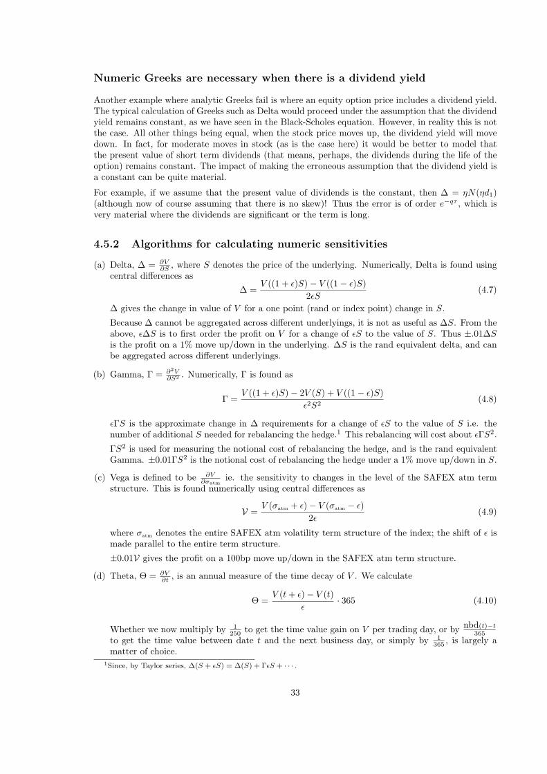
4.5.2 Algorithms for calculating numeric sensitivities

(a) Delta, ∆ = ∂V∂S , where S denotes the price of the underlying. Numerically, Delta is found using

central differences as

∆ =V ((1 + ε)S)− V ((1− ε)S)

2εS(4.7)

∆ gives the change in value of V for a one point (rand or index point) change in S.

Because ∆ cannot be aggregated across different underlyings, it is not as useful as ∆S. From theabove, ε∆S is to first order the profit on V for a change of εS to the value of S. Thus ±.01∆Sis the profit on a 1% move up/down in the underlying. ∆S is the rand equivalent delta, and canbe aggregated across different underlyings.

(b) Gamma, Γ = ∂2V∂S2 . Numerically, Γ is found as

Γ =V ((1 + ε)S)− 2V (S) + V ((1− ε)S)

ε2S2(4.8)

εΓS is the approximate change in ∆ requirements for a change of εS to the value of S i.e. thenumber of additional S needed for rebalancing the hedge.1 This rebalancing will cost about εΓS2.

ΓS2 is used for measuring the notional cost of rebalancing the hedge, and is the rand equivalentGamma. ±0.01ΓS2 is the notional cost of rebalancing the hedge under a 1% move up/down in S.

(c) Vega is defined to be ∂V∂σatm

ie. the sensitivity to changes in the level of the SAFEX atm termstructure. This is found numerically using central differences as

V =V (σatm + ε)− V (σatm − ε)

2ε(4.9)

where σatm denotes the entire SAFEX atm volatility term structure of the index; the shift of ε ismade parallel to the entire term structure.

±0.01V gives the profit on a 100bp move up/down in the SAFEX atm term structure.

(d) Theta, Θ = ∂V∂t , is an annual measure of the time decay of V . We calculate

Θ =V (t + ε)− V (t)

ε· 365 (4.10)

Whether we now multiply by 1250 to get the time value gain on V per trading day, or by nbd(t)−t

365to get the time value between date t and the next business day, or simply by 1

365 , is largely amatter of choice.

1Since, by Taylor series, ∆(S + εS) = ∆(S) + ΓεS + · · · .

33

Also, there are two different possible assumptions about what happens to S as time moves forward.The one is that S remains constant, so θ is calculated without moving S. The other is that Srolls up the forward curve, so in the shadow calculation we replace S with Serε, and also takeinto account any dividend payments.

(e) Rho, ρ = ∂V∂r , where r denotes the input risk free rate NACC. These are found from a standard

NACC yield curve. In the case of multiple input risk free rates, ρ is the sensitivity to a simulta-neous (parallel) shift in the entire term structure. ρ is found numerically using central differencesas

ρ =V (r + ε)− V (r − ε)

2ε(4.11)

±0.01ρ gives the profit on a 100bp NACC parallel move up/down in the term structure.

4.5.3 Taylor series

Consider a first order (delta-gamma-rho-vega-theta) Taylor series expansion as follows:

dV ' ∆ δS + 12Γ (δS)2 + ρ δr + V δσatm + θ δt

This expansion allows us to attribution our p&l according to the sensitivities, and this enables us toanalyse what type of bets the dealer is making.

For a simple instrument, such as an equity derivative, we can attribute the p&l as

• ∆t−1 (St − St−1) is the p&l due to delta;

• 12Γt−1 (St − St−1)2 is the p&l due to gamma;

• ρt−1 (rt − rt−1) is the p&l due to rho;

• Vt−1 (σatm,t − σatm,t−1) is the p&l due to vega;

• θt−1 δt is the p&l due to theta;

• the remainder is the p&l due to error in the Taylor series expansion.

At regular intervals we should check that the error term is not material. Of course, we can attribute apercentage to this error term, which should not be more than a couple of percent. After all, the errorterm is a measure of how well the Taylor series expansion is fitting the actual p&l. As expected, formore complicated products, these errors can be more material, and the method should not be used.Alternatively, a higher order Taylor series expansion could be derived and the appropriate attributionrecalculated.

Another possible occasion when the attribution will be less satisfactory is during market turbulence,when the moves δS, δr, etc. are large.

34

Chapter 5

The regulatory environment

5.1 Backtesting

If the relevant regulatory body gives its approval, a bank can use its own internal VaR calculation asa basis for capital adequacy, rather than another more punitive measure that must be used by banksthat do not have such approval.

The internal models approach is the most desirable method for determining capital adequacy.1 Thequantification of market risk for capital adequacy is determined by the bank’s own VaR model.However, given a free hand, a bank could simply understate their VaR. Hence, there is a need to testthe model to see if the stated VaR is consistent with the p&l that actually occurs. This is the purposeof backtesting, which applies statistical tests to see if the number of exceptions that have occurred isconsistent with the number of exceptions predicted by the model.

To find the market risk charge under VaR, we first determine the 10 trading day (or two week) VaRat the 99% confidence level, call it VaR10. The Market Risk Charge at time t is

max{VaR10

t−1, k ·Ave(VaR10

t−1, VaR10t−2, . . . , VaR10

t−60

)}(5.1)

where k can be as low as 3 but may be increased to as much as 4 if backtesting proves unsatisfactoryie. backtesting reveals that a bank is overly optimistic in the estimates of VaR. This provision isclearly to prevent gaming by the bank - under-reporting VaR numbers (in the expectation that theywill not backtest) in order to lower capital requirements.

The factor k ≈ 3 comes from thin air - the so-called hysteria factor. Legend has it that it arose as acompromise between the US regulatory authorities (who wanted k = 1) and the German authorities(who wanted k = 5) (Dowd 1998).

In principle the correct approach would be to measure the VaR at the holding period and confidencelevel that maps to the preferred probability of institutional survival (eg. 1 year and 99.75% for an Arated bank) and then use k = 1 (Dowd 1998).

The 10-day VaR is actually calculated using a 1-day VaR and the square root of time rule. In thiscase the Market Risk Charge at time t is

√10max

{VaR1

t−1, k ·Ave(VaR1

t−1, VaR1t−2, . . . , VaR1

t−60

)}(5.2)

where the VaR numbers are now with daily horizon.1We are specifically referring here to market risk capital requirements. To obtain regulatory approval to use an

internal model, the institution also has to have in place tested measures for credit risk and operational risk. That is notthe subject of this document. For an overview of the entire regulatory process, known as Basel II, see (Basel Committeeon Banking Supervision 2003), (Basel Committee on Banking Supervision 2004b).

35

The actual regulatory capital requirement will also include a Specific Risk Charge for issuer-specificrisks, such as credit risks. In Basle II operational risk charges are included.

In an interesting study done in 1996, at the time these proposals were being made into regulations,(Dimson & Marsh 1996) found that the internal models approach was the only method that wasconsistently sufficient to safeguard the capital of banks in times of stress. They also found that amethod they call net capital at risk, which can be viewed as a misapplication of a VaR-type approach,was by far the worst of the several methods examined. This would be, for example, a pure net deltaapproach to VaR - as would occur if a South African bank was to use a delta equivalent positionin the TOP40 for their entire set of domestic equity-based positions. Thus, they conclude that theinternal models approach only makes sense with stringent quality control.

An exception is a day on which the loss amount was greater than the VaR amount. If we are workingwith a 95% confidence, and if the model is accurate, then on average we should have an exception on1 day out of 20.

Even though Capital Adequacy is based on 99% VaR with a 10-day holding period, backtesting isperformed on VaR with a daily horizon, and can be performed at other confidence levels. There isno theoretical problem with this, and the advantage of using daily VaR is that a larger sample isavailable and so statistical tests have greater power. Of course the horizon cannot be less than thefrequency of p&l reporting, and this is almost always daily.

Backtesting is a logical manner of providing suitable incentives for use of internal models.

The question arises as to whether to use actual or theoretical p&l’s. It is often argued that VaRmeasures cannot be compared against actual trading outcomes, since the actual outcomes are con-taminated by changes in portfolio composition, and more specifically intra-day trading. This problembecomes more severe the longer the holding period, and so the backtesting framework involves one-dayVaR.

To the extent that backtesting is purely an exercise in statistics, it is clear that the theoretical p&l’sshould be used for an uncontaminated test. However, what the regulator is really interested in isthe solvency of the institution in reality, not in a theoretical world! Thus there are arguments forboth approaches, and in fact backtesting has been a requirement for approved VaR models since thebeginning of 1999, on both an actual (traded) and theoretical (hypothetical) basis. This is to ensurethat the model is continually evaluated for reasonability. Backtesting for approved models occurs ona quarterly basis with one year of historical data (250 trading days) as input.

Extensive backtesting guidelines are given in the January 1997 Basle accord (Basel Committee onBanking Supervision 1996b).

Because of the statistical limitations of backtesting the Basle committee introduced a three zoneapproach:

• Green zone: the test does not raise any concerns about the model. The test results are consistentwith an accurate model.

• Yellow zone: the test raises concerns about the model, but the evidence is not conclusive. Thetest results could be consistent with either an accurate or inaccurate model.

The capital adequacy factor (k-factor) will be increased by the regulator. The placement in theyellow zone (closer to green or red) should guide the increase in a firms capital requirement.The following recommendations are made (Basel Committee on Banking Supervision 1996b):

36

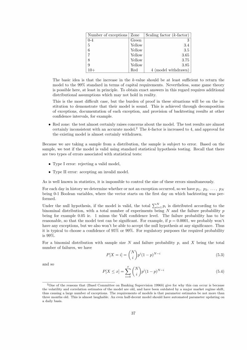
Number of exceptions Zone Scaling factor (k-factor)0-4 Green 35 Yellow 3.46 Yellow 3.57 Yellow 3.658 Yellow 3.759 Yellow 3.8510+ Red 4 (model withdrawn)

The basic idea is that the increase in the k-value should be at least sufficient to return themodel to the 99% standard in terms of capital requirements. Nevertheless, some game theoryis possible here, at least in principle. To obtain exact answers in this regard requires additionaldistributional assumptions which may not hold in reality.

This is the most difficult case, but the burden of proof in these situations will be on the in-stitution to demonstrate that their model is sound. This is achieved through decompositionof exceptions, documentation of each exception, and provision of backtesting results at otherconfidence intervals, for example.

• Red zone: the test almost certainly raises concerns about the model. The test results are almostcertainly inconsistent with an accurate model.2 The k-factor is increased to 4, and approval forthe existing model is almost certainly withdrawn.

Because we are taking a sample from a distribution, the sample is subject to error. Based on thesample, we test if the model is valid using standard statistical hypothesis testing. Recall that thereare two types of errors associated with statistical tests:

• Type I error: rejecting a valid model,

• Type II error: accepting an invalid model.

As is well known in statistics, it is impossible to control the size of these errors simultaneously.

For each day in history we determine whether or not an exception occurred, so we have p1, p2, . . . , pN

being 0-1 Boolean variables, where the vector starts on the first day on which backtesting was per-formed.

Under the null hypothesis, if the model is valid, the total∑N

i=1 pi is distributed according to thebinominal distribution, with a total number of experiments being N and the failure probability pbeing for example 0.05 ie. 1 minus the VaR confidence level. The failure probability has to bereasonable, so that the model test can be significant. For example, if p = 0.0001, we probably won’thave any exceptions, but we also won’t be able to accept the null hypothesis at any significance. Thusit is typical to choose a confidence of 95% or 99%. For regulatory purposes the required probabilityis 99%.

For a binomial distribution with sample size N and failure probability p, and X being the totalnumber of failures, we have

P [X = i] =(

N

i

)pi(1− p)N−i (5.3)

and so

P [X ≤ x] =x∑

i=0

(N

i

)pi(1− p)N−i (5.4)

2One of the reasons that (Basel Committee on Banking Supervision 1996b) give for why this can occur is becausethe volatility and correlation estimates of the model are old, and have been outdated by a major market regime shift,thus causing a large number of exceptions. The requirements of models is that parameter estimates be not more thanthree months old. This is almost laughable. An even half-decent model should have automated parameter updating ona daily basis.

37

Figure 5.1: Diagrammatic representation of the three zone approach for 95% VaR

We reject the null hypothesis if the number of exceptions is larger than the test level. There are twotest levels which correspond to the yellow and red zones. The yellow zone is determined by the BasleAccord as having a 5% Type I error. Thus, if the VaR model is valid, there is only a 5% chance of itbeing in the yellow zone - in other words, bad luck in terms of the number of exceptions. The red zoneis defined by the Basle Accord as having a 0.01% Type I error. Thus if the VaR model is valid, thereis only a 0.01% chance that it will have this number of exceptions. This is very generous, because oneconcludes that once a possibly suspect (but not absurd) model has been approved, only a very poorperformance subsequently will lead to approval being withdrawn. The Basle regulations ensure thatType I errors are almost impossible, but it allows for a significant proportion of Type II errors.

On a sample of N = 250 observations, with a failure probability of 0.01, the yellow zone starts with5 exceptions and the red zone starts with 10 exceptions. Note that 2.5 exceptions are expected.

Presumably, in order to qualify as an approved model, it starts off life in the green zone. Thus, atthe time of inception, the daily VaR at the 99% confidence level had at most 4 exceptions. If, at anyquarter end, the previous 250 observations had from 5 to 9 exceptions, the model is reclassified intothe yellow zone. If it had 10 or more exceptions, it is reclassified into the red zone.

Warning: in many statistics textbooks normal distribution approximations are available for the bino-mial distribution. These are not to be used here, because they only apply for binominals where thefailure probability is ‘not too extreme’, for example, (Underhill & Bradfield 1994) specifies that thenormal approximation is only valid if 0.1 < p < 0.9. We are interested in the case where p = 0.05,p = 0.01 or perhaps p = 0.0001.

5.2 Other requirements for internal model approval

Banks that use the internal models approach for meeting market risk capital requirements must havein place a rigorous and comprehensive stress testing program. The stress scenarios need to cover arange of factors that can create extraordinary p&l’s in trading portfolios, or make the control of riskin those portfolios very difficult. These factors include low-probability events in all major types ofrisks, including the various components of market, liquidity, credit, and operational risks.

38

Figure 5.2: The yellow zone starts with 5 exceptions and the red zone starts with 10 exceptions for99% VaR.

The institution must be able to provide information as follows (Basel Committee on Banking Supervision1996a):

• Information on the largest losses experienced during the reporting period.

• Stress testing the current portfolio against past periods of significant disturbance, incorporatingboth the large price movements and the sharp reduction in liquidity associated with these events.

Stress testing the sensitivity of the bank’s exposure to changes in the assumptions about volatil-ities and correlations. Due consideration should be given to the sharp variation that at timeshas occurred in periods of significant market disturbance. The 1987 equity crash, for example,involved correlations within risk factors approaching the extreme values of 1 or -1 for severaldays at the height of the disturbance.

• Use of scenarios developed by the bank itself to capture the specific characteristics of its portfolio.Banks should provide supervisory authorities with a description of the methodology used toidentify and carry out the scenarios as well as with a description of the results derived fromthese scenarios.

If the testing reveals particular vulnerability to a given set of circumstances, the national authoritieswould expect the bank to take prompt steps to manage those risks appropriately (eg. by hedgingagainst that outcome or reducing the size of its exposures).

5.3 Credit and operational risk measures

5.3.1 Basel I

(Basel Committee on Banking Supervision 1988). This was finalised in 1988, effective 1992.

We need to set a minimum level of risk capital, which is a percentage of the total risk weighted assets(RWA).

39

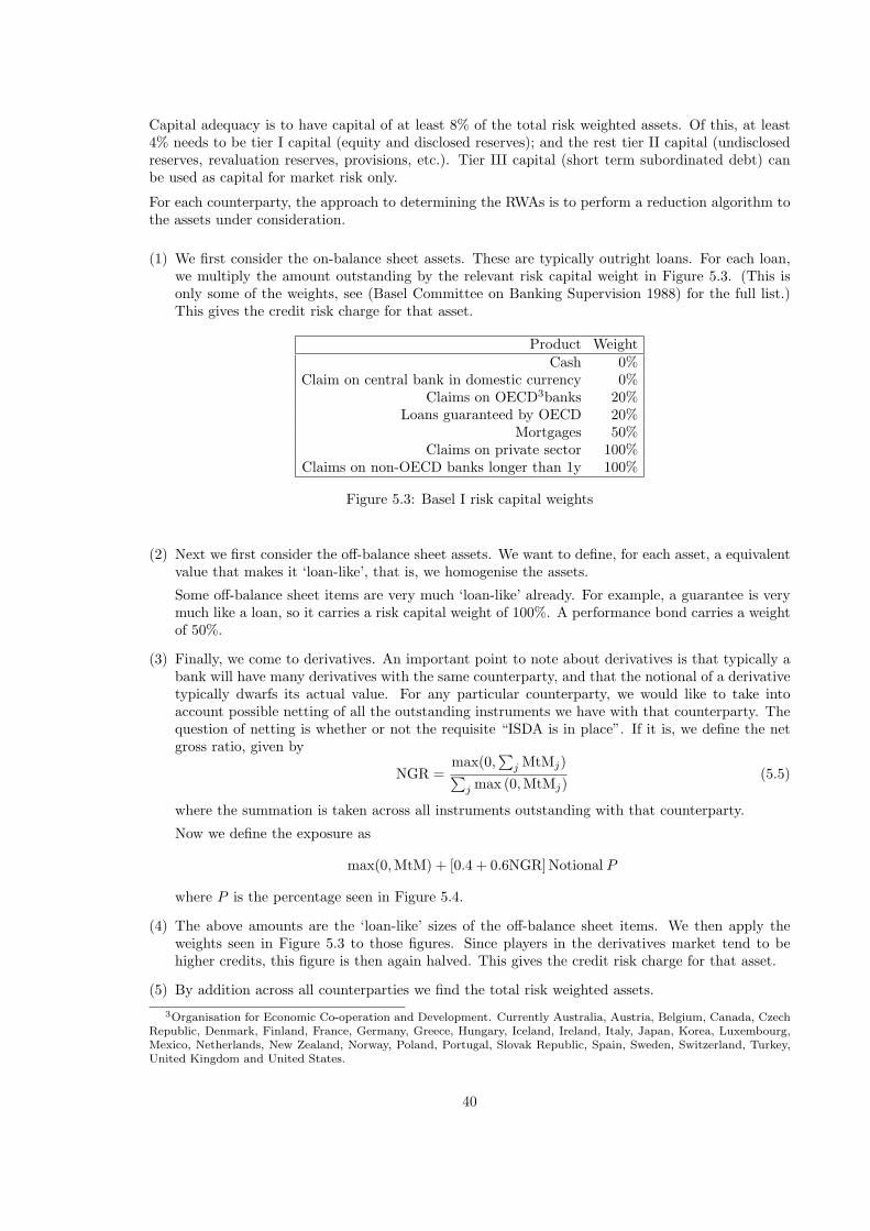
Capital adequacy is to have capital of at least 8% of the total risk weighted assets. Of this, at least4% needs to be tier I capital (equity and disclosed reserves); and the rest tier II capital (undisclosedreserves, revaluation reserves, provisions, etc.). Tier III capital (short term subordinated debt) canbe used as capital for market risk only.

For each counterparty, the approach to determining the RWAs is to perform a reduction algorithm tothe assets under consideration.

(1) We first consider the on-balance sheet assets. These are typically outright loans. For each loan,we multiply the amount outstanding by the relevant risk capital weight in Figure 5.3. (This isonly some of the weights, see (Basel Committee on Banking Supervision 1988) for the full list.)This gives the credit risk charge for that asset.

Product WeightCash 0%

Claim on central bank in domestic currency 0%Claims on OECD3banks 20%

Loans guaranteed by OECD 20%Mortgages 50%

Claims on private sector 100%Claims on non-OECD banks longer than 1y 100%

Figure 5.3: Basel I risk capital weights

(2) Next we first consider the off-balance sheet assets. We want to define, for each asset, a equivalentvalue that makes it ‘loan-like’, that is, we homogenise the assets.

Some off-balance sheet items are very much ‘loan-like’ already. For example, a guarantee is verymuch like a loan, so it carries a risk capital weight of 100%. A performance bond carries a weightof 50%.

(3) Finally, we come to derivatives. An important point to note about derivatives is that typically abank will have many derivatives with the same counterparty, and that the notional of a derivativetypically dwarfs its actual value. For any particular counterparty, we would like to take intoaccount possible netting of all the outstanding instruments we have with that counterparty. Thequestion of netting is whether or not the requisite “ISDA is in place”. If it is, we define the netgross ratio, given by

NGR =max(0,

∑j MtMj)∑

j max (0, MtMj)(5.5)

where the summation is taken across all instruments outstanding with that counterparty.

Now we define the exposure as

max(0, MtM) + [0.4 + 0.6NGR]Notional P

where P is the percentage seen in Figure 5.4.

(4) The above amounts are the ‘loan-like’ sizes of the off-balance sheet items. We then apply theweights seen in Figure 5.3 to those figures. Since players in the derivatives market tend to behigher credits, this figure is then again halved. This gives the credit risk charge for that asset.

(5) By addition across all counterparties we find the total risk weighted assets.

3Organisation for Economic Co-operation and Development. Currently Australia, Austria, Belgium, Canada, CzechRepublic, Denmark, Finland, France, Germany, Greece, Hungary, Iceland, Ireland, Italy, Japan, Korea, Luxembourg,Mexico, Netherlands, New Zealand, Norway, Poland, Portugal, Slovak Republic, Spain, Sweden, Switzerland, Turkey,United Kingdom and United States.

40

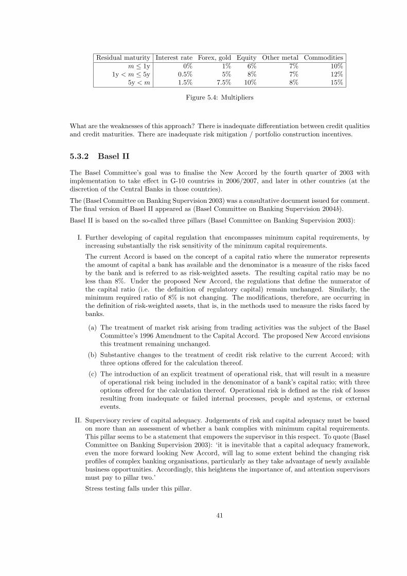
Residual maturity Interest rate Forex, gold Equity Other metal Commoditiesm ≤ 1y 0% 1% 6% 7% 10%

1y < m ≤ 5y 0.5% 5% 8% 7% 12%5y < m 1.5% 7.5% 10% 8% 15%

Figure 5.4: Multipliers

What are the weaknesses of this approach? There is inadequate differentiation between credit qualitiesand credit maturities. There are inadequate risk mitigation / portfolio construction incentives.

5.3.2 Basel II

The Basel Committee’s goal was to finalise the New Accord by the fourth quarter of 2003 withimplementation to take effect in G-10 countries in 2006/2007, and later in other countries (at thediscretion of the Central Banks in those countries).

The (Basel Committee on Banking Supervision 2003) was a consultative document issued for comment.The final version of Basel II appeared as (Basel Committee on Banking Supervision 2004b).

Basel II is based on the so-called three pillars (Basel Committee on Banking Supervision 2003):

I. Further developing of capital regulation that encompasses minimum capital requirements, byincreasing substantially the risk sensitivity of the minimum capital requirements.

The current Accord is based on the concept of a capital ratio where the numerator representsthe amount of capital a bank has available and the denominator is a measure of the risks facedby the bank and is referred to as risk-weighted assets. The resulting capital ratio may be noless than 8%. Under the proposed New Accord, the regulations that define the numerator ofthe capital ratio (i.e. the definition of regulatory capital) remain unchanged. Similarly, theminimum required ratio of 8% is not changing. The modifications, therefore, are occurring inthe definition of risk-weighted assets, that is, in the methods used to measure the risks faced bybanks.

(a) The treatment of market risk arising from trading activities was the subject of the BaselCommittee’s 1996 Amendment to the Capital Accord. The proposed New Accord envisionsthis treatment remaining unchanged.

(b) Substantive changes to the treatment of credit risk relative to the current Accord; withthree options offered for the calculation thereof.

(c) The introduction of an explicit treatment of operational risk, that will result in a measureof operational risk being included in the denominator of a bank’s capital ratio; with threeoptions offered for the calculation thereof. Operational risk is defined as the risk of lossesresulting from inadequate or failed internal processes, people and systems, or externalevents.

II. Supervisory review of capital adequacy. Judgements of risk and capital adequacy must be basedon more than an assessment of whether a bank complies with minimum capital requirements.This pillar seems to be a statement that empowers the supervisor in this respect. To quote (BaselCommittee on Banking Supervision 2003): ‘it is inevitable that a capital adequacy framework,even the more forward looking New Accord, will lag to some extent behind the changing riskprofiles of complex banking organisations, particularly as they take advantage of newly availablebusiness opportunities. Accordingly, this heightens the importance of, and attention supervisorsmust pay to pillar two.’

Stress testing falls under this pillar.

41

III. Public disclosure (market discipline). Again, from (Basel Committee on Banking Supervision2003): ’The Committee has sought to encourage market discipline by developing a set of disclo-sure requirements that allow stakeholders to assess key information about a bank’s risk profileand level of capitalisation.’ For example, annual reports to shareholders will have to includefairly solid evidence, adhering to some prescribed general formats, rather than qualitative me-anderings, about the methods of risk control.

Public disclosure strengthens the incentives for a bank to behave prudently.

Just how much control the regulator will have over the nature of this information will dependon the legal jurisdiction that applies to the particular regulator-bank relationship.

Countries not represented in the G-10 have more freedom in their implementation programme, andmany have been busy evaluating the suitability of the new Framework for their jurisdiction. In orderto further this process the committee convened a Working Group comprised of members from non-G10 countries to assess the whether and when of Basel II, and to provide practical suggestions tosupervisors for the transition to the new Framework. This occurred in the first half of 2003 withthe report being (Basel Committee on Banking Supervision 2004a). The document is not intendedto be an interpretation of Basel II rules, but rather as practical advise for countries with differingresources, particular concentration risks, etc. (Basel Committee on Banking Supervision 2003), (BaselCommittee on Banking Supervision 2004b). South Africa has an implementation target date of 1January 2008.

The first pillar of Basel II deals with the new methods for calculation of exposures. For credit riskthere are broadly two approaches:

(a) Standardised Approach: similar to Basel I in that banks are required to slot their credit exposuresinto supervisory categories. The categories can be determined as corresponding to the ratingcategories published by a rating agency. For example, we see in Figure 5.3 that any claim witha counterparty in the private sector has a risk weight of 100% under Basel I. In Basel II, if thecounterparty is rated anything from AAA to AA-, then the risk weight is 20%, A+ to A- is 50%,etc. Below B- is 150%.4

Another source of relief is that the risk weight for mortgages has been reduced. Also, somerecognition for protection from bought credit derivatives is available.

However, this approach is now very punitive in terms of the amount of capital that needs to beheld. Moreover, in South Africa the lack of many internationally rated corporates makes thismethod difficult to apply. Hence banks will be aiming for the internal ratings-based approach.

(b) The internal ratings-based approach.

(i) for corporate, bank and sovereign exposures. The bank will use a model where the riskcomponents are

• Probability of default (PD), a percentage• Loss given default (LGD), a percentage• Exposure at default (EAD), in currency units• Maturity (M), in years

The capital required will be proportional to

EAD · LGD · [s− PD] · f(M) (5.6)

where s is a parameter which is intended to cover unexpected losses at the 99.9% confidencelevel, and f a given increasing function with f(1) = 1.For the foundational internal ratings-based approach the PD is provided by the bank, theothers are set by the supervisor. For the advanced internal ratings-based approach all inputs

4Lest this doesn’t make sense, remember that we are going to multiply by 8% later on.

42

for an internal model are provided by the bank: these will be at least the factors listed above,there may be others. The loss given default is especially difficult for a bank to quantify, givenagain the small number of defaults historically, so banks here will typically pass this issueback to the regulator, and stick to the foundational model. Moreover, some research hasshown that in emerging markets, banks tends to have far higher concentration risk levels,and hence this method could be more punitive than would first appear! (Risk MagazineJune 2003). With the takeover of ABSA by Barclay’s, ABSA made a firm commitmentto implement the internal ratings-based approach, with the other big banks then makingcommitments to do likewise (Risk Magazine November 2005).Small/medium enterprise exposures with an exposure of more than €1m will be treated ascorporate exposures, with some firm-size adjustments.

(ii) for retail exposures. There is only one approach available. The bank provides all of PD,LGD and EAD; on a pooled basis, rather than on a name by name basis. The exposuresare divided into three categories, which is broadly mortgages, credit cards, and other. Theformula for capital required is the same as (5.6) except the maturity factor disappears foreach of these categories; the s factor is calibrated differently for each of the three categories.5

The capital required is then aggregated.Small/medium enterprise exposures with an exposure of less than €1m will be treated asretail exposures.

(iii) for specialised lending. There are two options: this is treated as a corporate exposure.Commercial retail estate has a special category. Alternatively, a scale of five quality gradeswith risk weights for each grade is available.

(iv) equity exposures. There are two options: a corporate approach is taken, but LGD is man-dated at 90%. Alternatively, a quarterly VaR type approach can be taken to model thepotential decrease in the value of equity holdings.

In the internal rating based approach, the bank needs to calculate the PD (under either of thetwo variations). For this Basel II sets certain requirements in the calculation methodology andtesting for PD estimates.

The requirement is that obligors are classified into risk buckets, and each risk bucket is assigned aPD. This PD must be a long-run average of the one-year realised default rates for that bucket. Assuch, it could vary significantly from a case-by-case model of obligor’s PDs that will result from(KMV 2006) for example. Basel also enunciates a preference for a through the cycle approachi.e. the PD is based on long term statistics and is not overly dependent on where we are in theeconomic cycle.

Although there is great freedom in the definition of the risk buckets, the benchmarking andbacktesting requirements of these buckets is quite stringent.

Calculation methods for operational risk:

1. Basic Indicator Approach: the measure is a bank’s average annual gross income over the previousthree years. This average, multiplied by a factor of 0.15 set by the Committee, produces thecapital requirement.

2. Standardised Approach: similar, but banks must calculate a capital requirement for each busi-ness line. This is determined by multiplying gross income by specific supervisory factors deter-mined by the Committee.

3. Advanced Measurement Approaches Fairly open ended specifications, stated as aimed to en-courage the growth of the quantification of operational risk. Banks using such methods arepermitted to recognise the risk mitigating impact of insurance.

5Both here and above the s factor has a modelled correlation within the group as a significant input.

43

The second two methods do not produce a significant saving over the first, so banks will typically optfor the first approach.

Credit Risk Market Risk Operational RiskBasel1988

Standardised approach Standardised approach -

Basel1996

Standardised approach St’disedapproach

Internalmodel(VaR,stress)

-

Basel2006++

St’disedapproach

Foun-dationalinternalratingapproach

AdvancedInternalratngapproach

St’disedapproach

Internalmodel(VaR,stress)

Basic in-dicatorapproach

St’disedapproach

Advancedmeasure-ment

44

Chapter 6

Coherent risk measures

6.1 VaR cannot be used for calculating diversification

If f is a risk measure, the diversification benefit of aggregating portfolio’s A and B is defined to be

f(A) + f(B)− f(A + B) (6.1)

When using full revaluation VaR as the methodology for computing a risk measure, it’s quite possibleto get negative diversification. Pathological examples are possible, but the following example is notabsurd:

Suppose one has a portfolio that is made up by a Trader A and Trader B. Trader A has a portfolioconsisting of a sold put that is far out of the money, and has one day to expiry. Trader B has aportfolio that consists of a sold call that is also far out of the money, and also has one day to expiry.Using any historical VaR approach, say we find that each option has a probability of 4% of ending upin the money.

Trader A and B each have a portfolio that has a 96% chance of not losing any money, so each has a95% VaR of zero.1 However, the combined portfolio has only a 92% chance of not losing any money,so its VaR is non-trivial. Therefore we have a case where the risk of the combined portfolio is greaterthan the risks associated with the individual portfolios, i.e. negative diversification benefit if VaRis used to measure the diversification benefit. This example appears in (Artzner, Delbaen, Eber &Heath 1997).

What is so awkward about the lack of sub-additivity is the fact that this can give rise to regulatoryarbitrage or to the break-down of global risk management within one single firm. This is also a seriousconcern for regulators. If regulation allows the capital requirement of a firm to be calculated as thesum of the requirements of its subsidiaries and if the requirements are based on VaR, the firm couldcreate artificial subsidiaries in order to save regulatory capital.

6.2 Risk measures and coherence

This example introduces the concept of a “Coherent Risk Measure”. If f(A+B) ≤ f(A)+f(B), whereA and B denote portfolios, then f is said to be coherent (Artzner et al. 1997), (Artzner, Delbaen, Eber& Heath 1999). In fact a coherent risk measure needs to satisfy five properties (Artzner et al. 1999),as follows:

1To be precise, their VaR is actually a very small negative number! The average of their Vi’s is negative, the 5th%is zero.

45

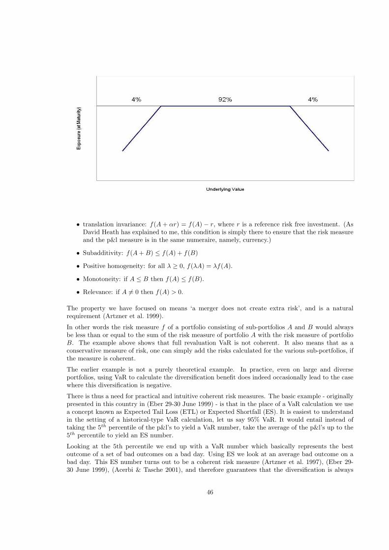
• translation invariance: f(A + αr) = f(A) − r, where r is a reference risk free investment. (AsDavid Heath has explained to me, this condition is simply there to ensure that the risk measureand the p&l measure is in the same numeraire, namely, currency.)

• Subadditivity: f(A + B) ≤ f(A) + f(B)

• Positive homogeneity: for all λ ≥ 0, f(λA) = λf(A).

• Monotoneity: if A ≤ B then f(A) ≤ f(B).

• Relevance: if A 6= 0 then f(A) > 0.

The property we have focused on means ‘a merger does not create extra risk’, and is a naturalrequirement (Artzner et al. 1999).

In other words the risk measure f of a portfolio consisting of sub-portfolios A and B would alwaysbe less than or equal to the sum of the risk measure of portfolio A with the risk measure of portfolioB. The example above shows that full revaluation VaR is not coherent. It also means that as aconservative measure of risk, one can simply add the risks calculated for the various sub-portfolios, ifthe measure is coherent.

The earlier example is not a purely theoretical example. In practice, even on large and diverseportfolios, using VaR to calculate the diversification benefit does indeed occasionally lead to the casewhere this diversification is negative.

There is thus a need for practical and intuitive coherent risk measures. The basic example - originallypresented in this country in (Eber 29-30 June 1999) - is that in the place of a VaR calculation we usea concept known as Expected Tail Loss (ETL) or Expected Shortfall (ES). It is easiest to understandin the setting of a historical-type VaR calculation, let us say 95% VaR. It would entail instead oftaking the 5th percentile of the p&l’s to yield a VaR number, take the average of the p&l’s up to the5th percentile to yield an ES number.

Looking at the 5th percentile we end up with a VaR number which basically represents the bestoutcome of a set of bad outcomes on a bad day. Using ES we look at an average bad outcome on abad day. This ES number turns out to be a coherent risk measure (Artzner et al. 1997), (Eber 29-30 June 1999), (Acerbi & Tasche 2001), and therefore guarantees that the diversification is always

46

positive. As stated in the abstract of (Acerbi & Tasche 2001), “Expected Shortfall (ES) in severalvariants has been proposed as remedy for the deficiencies of Value-at-Risk (VaR) which in general isnot a coherent risk measure”.

A readable account of these and related issues is (Acerbi, Nordio & Sirtori 2001).

One should report both VaR and ES, but use only ES to calculate and report diversification.

Note that because standard deviation is sub-additive the standard RiskMetrics simplification is co-herent:

σ2(X + Y ) = σ2(X) + σ2(Y ) + 2σ(X)σ(Y )ρ≤ σ2(X) + σ2(Y ) + 2σ(X)σ(Y )

= (σ(X) + σ(Y ))2

and soσ(X + Y ) ≤ σ(X) + σ(Y )

and henceVaR(X + Y ) ≤ VaR(X) + VaR(Y ),

which is the definition of subadditivity. The usual RiskMetrics VaR is also subadditive (and hencecoherent), but this is a mathematical exercise for masochists - it is not easy at all. According to(Breuer, Krenn & Pistovcak 2002) to guarantee sub-additivity of (presumably parametric) VaR,the value of the portfolio has to be a linear function of risk factors whose changes are ellipticallydistributed.

6.3 Measuring diversification

The diversification benefit of portfolio P0 is equal to

f

(n∑

i=1

Pi

)+ f(P0)− f

(n∑

i=0

Pi

)

where f denotes ES and P1, P2, . . . , Pn are the (original) portfolios against which the diversificationis measured.

6.4 Coherent capital allocation

The intention is to allocate capital costs in a coherent manner. This sounds like quite an otherworldlyexercise, but one can make the task quite concrete and ask: of my risk number (such as ES), howmuch (as a percentage, say) is due to each of my positions? Then, given my capital adequacy charges(which may or may not be calculated via an approved internal model!) I can allocate as a cost thecharges in those proportions to each of those desks.

Each desk can break down their own charges amongst their dealers, and management can decidewhere the greatest risk managment focus needs to lie.

(Denault 2001) has developed a method of allocating the risk capital costs to the various subportfoliosin a fair manner, yielding for each portfolio, a risk appraisal that takes diversification into account.We wish to thank Freddie Delbaen, who contributed significantly to that paper, for clarifying certainissues.

The approach of (Denault 2001) is axiomatic, starting from a risk measure which is coherent in theabove sense. We may specialise the results of (Denault 2001) to the case of the coherent ExpectedShortfall risk measure in which case his results become quite concrete.

An allocation method for risk capital is then said to be coherent if

47

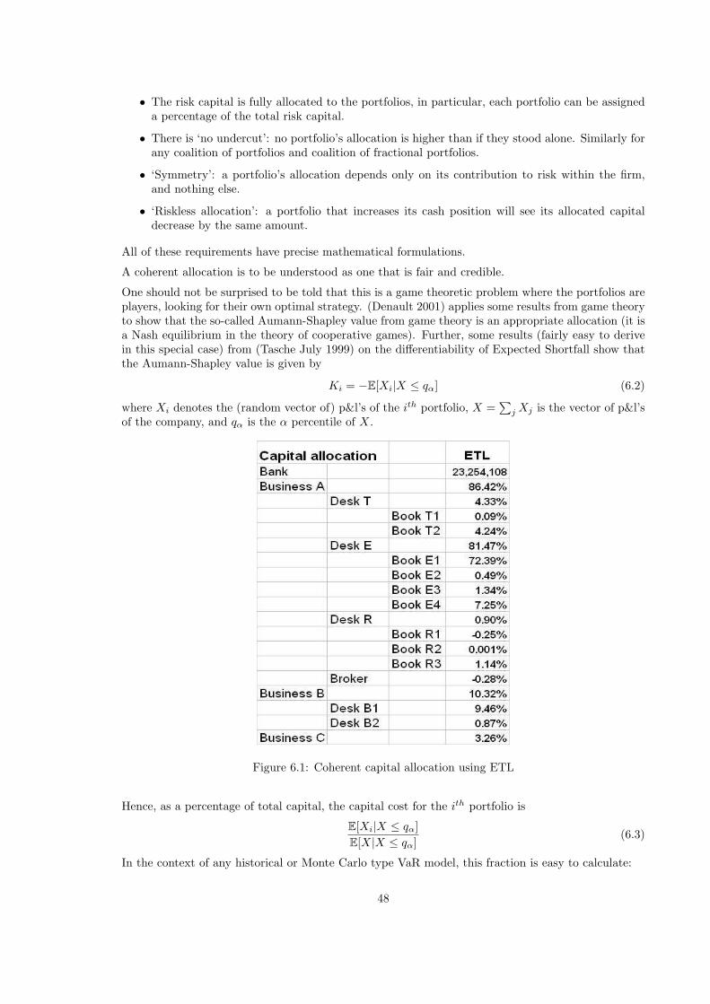
• The risk capital is fully allocated to the portfolios, in particular, each portfolio can be assigneda percentage of the total risk capital.

• There is ‘no undercut’: no portfolio’s allocation is higher than if they stood alone. Similarly forany coalition of portfolios and coalition of fractional portfolios.

• ‘Symmetry’: a portfolio’s allocation depends only on its contribution to risk within the firm,and nothing else.

• ‘Riskless allocation’: a portfolio that increases its cash position will see its allocated capitaldecrease by the same amount.

All of these requirements have precise mathematical formulations.

A coherent allocation is to be understood as one that is fair and credible.

One should not be surprised to be told that this is a game theoretic problem where the portfolios areplayers, looking for their own optimal strategy. (Denault 2001) applies some results from game theoryto show that the so-called Aumann-Shapley value from game theory is an appropriate allocation (it isa Nash equilibrium in the theory of cooperative games). Further, some results (fairly easy to derivein this special case) from (Tasche July 1999) on the differentiability of Expected Shortfall show thatthe Aumann-Shapley value is given by

Ki = −E[Xi|X ≤ qα] (6.2)

where Xi denotes the (random vector of) p&l’s of the ith portfolio, X =∑

j Xj is the vector of p&l’sof the company, and qα is the α percentile of X.

Figure 6.1: Coherent capital allocation using ETL

Hence, as a percentage of total capital, the capital cost for the ith portfolio is

E[Xi|X ≤ qα]E[X|X ≤ qα]

(6.3)

In the context of any historical or Monte Carlo type VaR model, this fraction is easy to calculate:

48

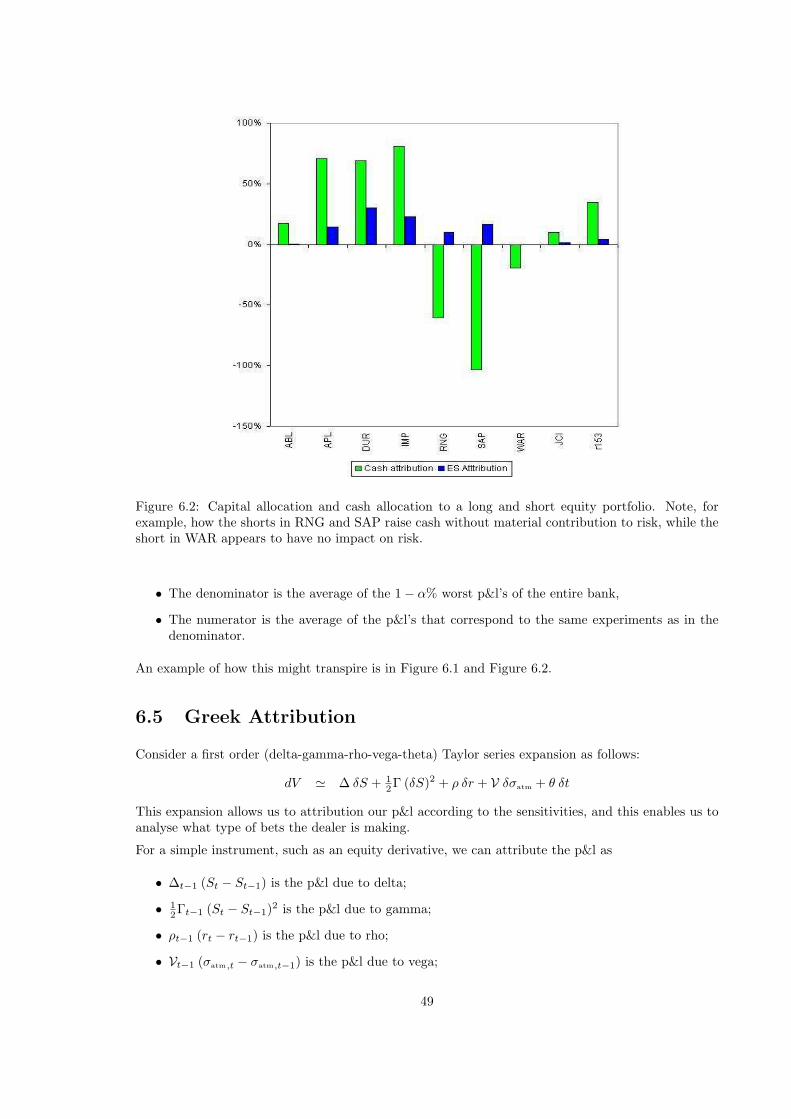
Figure 6.2: Capital allocation and cash allocation to a long and short equity portfolio. Note, forexample, how the shorts in RNG and SAP raise cash without material contribution to risk, while theshort in WAR appears to have no impact on risk.

• The denominator is the average of the 1− α% worst p&l’s of the entire bank,

• The numerator is the average of the p&l’s that correspond to the same experiments as in thedenominator.

An example of how this might transpire is in Figure 6.1 and Figure 6.2.

6.5 Greek Attribution

Consider a first order (delta-gamma-rho-vega-theta) Taylor series expansion as follows:

dV ' ∆ δS + 12Γ (δS)2 + ρ δr + V δσatm + θ δt

This expansion allows us to attribution our p&l according to the sensitivities, and this enables us toanalyse what type of bets the dealer is making.

For a simple instrument, such as an equity derivative, we can attribute the p&l as

• ∆t−1 (St − St−1) is the p&l due to delta;

• 12Γt−1 (St − St−1)2 is the p&l due to gamma;

• ρt−1 (rt − rt−1) is the p&l due to rho;

• Vt−1 (σatm,t − σatm,t−1) is the p&l due to vega;

49

• θt−1 δt is the p&l due to theta;

• the remainder is the p&l due to error in the Taylor series expansion.

At regular intervals we should check that the error term is not material. Of course, we can attribute apercentage to this error term, which should not be more than a couple of percent. After all, the errorterm is a measure of how well the Taylor series expansion is fitting the actual p&l. As expected, formore complicated products, these errors can be more material, and the method should not be used.Alternatively, a higher order Taylor series expansion could be derived and the appropriate attributionrecalculated.

Another possible occasion when the attribution will be less satisfactory is during market turbulence,when the moves δS, δr, etc. are large.

Now suppose that we wish to decompose a VaR or ES measure into exposures to the various Greeks.Assume that we are using a historical-type or Monte Carlo method for calculating our VaR or ES.Then we can consider the p&l’s generated by the various historical or Monte Carlo experiments, asfollows:

dVi = ∆(Si − S) + 12Γ(Si − S)2 + ρ(ri − r) + V(σatmi − σatm) + θδt + εi

where S is the original spot, Si is the ith spot experiment, etc. The p&l’s due to delta are the∆(Si − S), etc.

Of course, our risk measure is calculated by looking at the tail of this distribution of p&l’s.

Figure 6.3: Coherent greek attribution using ES

Again we should check that the εi are not material. This time it is even easier than before: the capitalattribution method is attributing a percentage to this error term, which should not be more than acouple of percent.

50

Bibliography

Acerbi, C., Nordio, C. & Sirtori, C. (2001), ‘Expected shortfall as a tool for financial risk management’.*http://www.gloriamundi.org/var/wps.html

Acerbi, C. & Tasche, D. (2001), ‘On the coherence of expected shortfall’.*http://www-m1.mathematik.tu-muenchen.de/m4/Papers/Tasche/shortfall.pdf

Artzner, P., Delbaen, F., Eber, J.-M. & Heath, D. (1997), ‘Thinking coherently’, Risk 10(11), 68–71.

Artzner, P., Delbaen, F., Eber, J.-M. & Heath, D. (1999), ‘Coherent measures of risk’, Math. Finance9(3), 203–228.*http://www.math.ethz.ch/~delbaen

Basel Committee on Banking Supervision (1988), ‘International convergence of capital measurementand capital standards (July 1988, updated to April 1998)’.*http://www.bis.org/publ/bcbsc111.pdf

Basel Committee on Banking Supervision (1996a), ‘Amendment to the capital accord to incorporatemarket risks’.*http://www.bis.org/publ/bcbs24.htm

Basel Committee on Banking Supervision (1996b), ‘Supervisory framework for the use of ‘backtesting’in conjunction with the internal models approach to market risk capital requirements’.*http://www.bis.org/publ/bcbs22.htm

Basel Committee on Banking Supervision (2003), ‘Consultative document: Overview of the new Baselcapital accord’.*http://www.bis.org/publ/cp3ov.pdf

Basel Committee on Banking Supervision (2004a), ‘Implementation of Basel II: Practical considera-tions’.*http://www.bis.org/publ/bcbs109.pdf

Basel Committee on Banking Supervision (2004b), ‘International convergence of capital measurementand capital standards: A revised framework’.*http://www.bis.org/publ/bcbs107.pdf

Breuer, T., Krenn, G. & Pistovcak, F. (2002), Stress tests, maximum loss, and value at risk,in B. Britzelmaier, S. Geberl, M. Menichetti & H.-R. Kaufmann, eds, ‘Regulierung oderDeregulierung der Finanzmrkte: Strategieimplikationen fr Finanzdienstleister’, Physica-Verlag(Springer).

Burden, R. L. & Faires, J. D. (1997), Numerical Analysis, sixth edn, Brooks Cole.

Denault, M. (2001), ‘Coherent allocation of risk capital’, Journal of Risk 4(1), 1–34.

Dimson, E. & Marsh, P. (1996), ‘Stress tests of capital requirements’, The Wharton School 96-50.

51

Dowd, K. (1998), Beyond Value at Risk: The new science of risk management, Wiley series in Frontiersof Finance, John Wiley and Sons.

Duffie, D. & Singleton, K. (2000), ‘Credit risk pricing and risk measurement for financial institutions’.Graduate School of Business, Stanford University.

Eber, J.-M. (29-30 June 1999), ‘Measures of risk for effective risk management’. Talk, Risk Confer-ences, Advanced techniques and strategies for risk measurement and management of derivatives,Johannesburg.

Fender, I., Gibson, M. & Mosser, P. (November 2001), ‘An international survey of stress tests’, CurrentIssues in Economics and Finance 7(10).

Higham, N. J. (2002), ‘Computing the nearest correlation matrix - a problem from finance’, IMAJournal of Numerical Analysis 22, 329–343.*http://www.ma.man.ac.uk/ nareports/narep369.pdf

Hosoya, M. & Shimizu, T. (December 2002), ‘Implications of a macro stress test on financial stability:Summary of the second census on stress tests’, Market Review, Bank of Japan Financial MarketsDepartment 2002-E-4.

Hull, J. (2002), Options, Futures, and Other Derivatives, fifth edn, Prentice Hall.

Hull, J. & White, A. (1998), ‘Incorporating volatility up-dating into the historical simulation methodfor V@R’, Journal of Risk 1(Fall).

J.P.Morgan & Reuters (December 18, 1996), RiskMetrics - Technical Document, fourth edn,J.P.Morgan and Reuters, New York.*http://www.riskmetrics.com

KMV (2006), ‘Moody’s KMV’.*http://www.moodyskmv.com/

Kolman, J. (April 1999), ‘LTCM speaks’, Derivatives Strategy .*http://www.derivativesstrategy.com/magazine/archive/1999/0499fea1.asp

Lowenstein, R. (2000), When Genius Failed: The Rise and Fall of Long Term Capital Management,Random House.

Mina, J. & Ulmer, A. (April 1999), ‘Delta-gamma four ways’, CreditMetrics Monitor .*http://www.riskmetrics.com/deltaow.html

Pafka, S. & Kondor, I. (2001), ‘Evaluating the RiskMetrics methodology in measuring volatility andvalue-at-risk in financial markets’.*http://www.colbud.hu/pdf/Kondor/riskm.pdf

Paul-Choudhury, S. (1997), ‘This year’s model’, Risk 10, 18–23.

Pichler, S. & Selitsch, K. (2000), ‘A comparison of analytical VaR methodologies for portfolios thatinclude options’, Model Risk .

Risk Magazine (June 2003), ‘South Africa special report’.

Risk Magazine (November 2005), ‘South Africa special report’.

Sharpe, W. F. (1964), ‘Capital asset prices - a theory of market equilibrium under conditions of risk’,Journal of Finance pp. 425–442.

Taleb, N. (1997), Dynamic Hedging: managing vanilla and exotic options, John Wiley and Sons.

52

Tasche, D. (July 1999), ‘Risk contributions and performance measurement’, Technische UniversitatMunchen TUM-M9909.

The Financial Economists Roundtable (October 6, 1999), ‘The financial economists roundtable state-ment on Long-Term Capital Management and the report of the presidents’ working group onfinancial markets’.*http://www.luc.edu/orgs/finroundtable/statement99.html

Underhill, L. & Bradfield, D. (1994), IntroSTAT, Juta and Company.

Wee, L.-S. & Lee, J. (1999), ‘Integrating stress testing with risk management’, Bank Accounting andFinance Spring, 7–19.

West, G. (2006), ‘The Mathematics of South African Financial Markets and Instruments: Lecturenotes’.*http://www.finmod.co.za/safm.pdf

Zangari, P. (1996), ‘A VaR methodology for portfolios that include options’, RiskMetrics MonitorFirst Quarter.

53