Risk Management: A Review - CFA Institute

©2009 The Research Foundation of CFA Institute 1

The Research Foundation of CFA Institute Literature Review

Risk Management: A ReviewSébastien Lleo, CFAImperial College London

The concept of risk has been central to the theory and practice of finance since Markowitz’s influentialwork nearly 60 years ago. Yet, risk management has only emerged as a field of independent study in thepast 15 years. Advances in the science of risk measurement have been a main contributor to this remarkabledevelopment as new risk measures have been proposed and their properties studied. These measures, whichin the past have only applied to market risk, are now being applied to credit, operational, and liquidityrisk as well as to portfolio optimization. A growing emphasis on risk budgeting has also sparked a questfor an integrated risk measurement framework. But risk management is more than the application ofquantitative techniques. A long list of past financial disasters demonstrates that a profound and concreteunderstanding of the nature of risk is required and that adequate internal controls are crucial.

The modern study of risk can be traced to Markowitz’s seminal work on portfolio selection.1 Markowitz madethe observation that one should care about risk as well as return, and he placed the study of risk at center stage inthe new field of financial economics. Since then, the science of risk management has grown and become its ownfield of study.

Initially, risk management was manifest in hedging, that is the elimination of unwanted aspects of risk. Hedgingis accomplished primarily through the use of derivatives. (An example would be the hedging of foreign currency riskassociated with purchasing foreign currency denominated securities.) In the past 15 years, however, risk managementhas evolved beyond the practice of hedging and into a complex discipline that revolves around two dimensions: riskmeasurement and the practice of risk management. The two disciplines are different in their connotations for andapplications to the various sectors of the financial industry. For investment banks and commercial banks, riskmanagement is instrumental in managing bank liquidity reserves and regulatory required capital. For active assetmanagement firms, it is a powerful tool for generating more efficient portfolios and higher alphas. These differencesreveal that risk measurement and risk management are not fixed ideas but customizable instruments that variousfirms use in different ways to add value by mitigating the financial effects of possible adverse events.

Today, a distinction can be made between portfolio risk management (as begun by Markowitz) and enterpriserisk management. Although these two disciplines are closely related through the shared goal of mitigating risk,they often involve the use of different tools and require different ways of thinking. This literature review willdiscuss both disciplines, but it will tilt toward a discussion of enterprise risk management. An extensive body ofliterature on portfolio risk management already exists.2

This review will address the following key questions:• What types of risk are financial market participants exposed to?• What lessons can be learned from past financial disasters to improve risk management?• What are the popular risk measures, how appropriate are they, and how are they best applied?• How are credit risk, operational risk, and liquidity risk measured?• What are the desirable properties of risk measures?• Why is the search for an integrated risk management framework important?

1See Markowitz (1952, 1959).2See, for example, Grinold and Kahn (1999).

Risk Management

2 ©2009 The Research Foundation of CFA Institute

Financial Risk or Financial Risks? Financial risk is not a monolithic entity. In fact, the classic view of risk categorizes it into several broad types:market, credit, operational, liquidity, and legal and regulatory. This classic view has provided a backbone for thephenomenal development of the science of risk management in the past 15 years. More than a scholarly attemptat organizing the universe, the categories reveal fundamental differences in the economics of each type of risk. Inmany financial institutions, these categories are also reflected in the organization of the risk management function.

Market risk is generally defined as the risk of a decline in asset prices as a result of unexpected changes inbroad market factors related to equity, interest rates, currencies, or commodities. Market risk is probably the bestunderstood type of risk and the type for which large amounts of good quality data are the most readily available.A variety of measures, such as value at risk, is readily available to evaluate market risk.

Credit risk measures the possibility of a decline in an asset price resulting from a change in the credit qualityof a counterparty or issuer (e.g., counterparty in an OTC transaction, issuer of a bond, reference entity of a creditdefault swap). Credit risk increases when the counterparty’s perceived probability of default or rating downgradeincreases. Five main credit risk measurement methodologies are discussed in this review (see the section “CreditRisk Methodologies”).

Operational risk is defined by the Basel Committee as “the risk of loss resulting from inadequate or failedinternal processes, people and systems, or from external events.”3 Thus, operational risk can result from suchdiverse causes as fraud, inadequate management and reporting structures, inaccurate operational procedures, tradesettlement errors, faulty information systems, or natural disaster.

Liquidity risk is the risk of being unable to either raise the necessary cash to meet short-term liabilities (i.e.,funding liquidity risk), or buy or sell a given asset at the prevailing market price because of market disruptions(i.e., trading-related liquidity risk). The two dimensions are interlinked because to raise cash to repay a liability(funding liquidity risk), an institution might need to sell some of its assets (and incur trading-related liquidity risk).

Legal and regulatory risk is the risk of a financial loss that is the result of an erroneous application of currentlaws and regulations or of a change in the applicable law (such as tax law).

The publication of numerous articles, working papers, and books has marked the unparalleled advances inrisk management. As a general reference, the following are a few of the sources that offer thorough treatments ofrisk management.

Das (2005) provided a general overview of the practice of risk management, mostly from the perspective ofderivatives contracts.

Embrechts, Frey, and McNeil (2005) emphasized the application of quantitative methods to risk management.Crouhy, Galai, and Mark (2001, 2006) are two solid risk management references for practitioners working

at international banks with special attention given to the regulatory framework.Jorion (2007) gave an overview of the practice of risk management through information on banking

regulations, a careful analysis of financial disasters, and an analysis of risk management pitfalls. He also made astrong case for the use of value-at-risk-based risk measurement and illustrated several applications and refinementsof the value-at-risk methodology.

Finally, Bernstein (1998) is another key reference. This masterpiece gives a vibrant account of the history ofthe concept of risk from antiquity to modern days.

3“International Convergence of Capital Measurement and Capital Standards,” Basel Committee on Banking Supervision, Bank forInternational Settlements (2004).

Risk Management


Lessons from Financial DisastersRisk management is an art as much as a science. It reflects not only the quantification of risks through riskmeasurement but also a more profound and concrete understanding of the nature of risk. The study of past financialdisasters is an important source of insights and a powerful reminder that when risks are not properly understoodand kept in check, catastrophes may easily occur. Following is a review of some past financial disasters.

Metallgesellschaft Refining and Marketing (1993). Although dated, the story of theMetallgesellschaft Refining and Marketing (MGRM) disaster is still highly relevant today because it is a complexand passionately debated case. Questions remain, such as was MGRM’s strategy legitimate hedging or speculation?Could and should the parent company, Metallgesellschaft AG, have withstood the liquidity pressure? Was thedecision to unwind the strategy in early 1994 the right one? If the debates about the MGRM disaster show usanything, it is that risk management is more than an application of quantitative methods and that key decisionsand financial strategies are open to interpretation and debate.

In December 1991, MGRM, the U.S.–based oil marketing subsidiary of German industrial groupMetallgesellschaft AG, sold forward contracts guaranteeing its customers certain prices for 5 or 10 years. By 1993,the total amount of contracts outstanding was equivalent to 150 million barrels of oil-related products. If oil pricesincreased, this strategy would have left MGRM vulnerable.

To hedge this risk, MGRM entered into a series of long positions, mostly in short-term futures (some forjust one month). This practice, known as “stack hedging,” involves periodically rolling over the contracts as theynear maturity to maintain the hedge. In theory, maintaining the hedged positions through the life of the long-term forward contracts eliminates all risk. But intermediate cash flows may not match, which would result inliquidity risk. As long as oil prices kept rising or remained stable, MGRM would be able to roll over its short-term futures without incurring significant cash flow problems. Conversely, if oil prices declined, MGRM wouldhave to make large cash infusions in its hedging strategy to finance margin calls and roll over its futures.

In reality, oil prices fell through 1993, resulting in a total loss of $1.3 billion on the short-term futures by theend of the year. Metallgesellschaft AG’s supervisory board took decisive actions by replacing MGRM’s seniormanagement and unwinding the strategy at an enormous cost. Metallgesellschaft AG was only saved by a $1.9billion rescue package organized in early 1994 by 150 German and international banks.

Mello and Parsons’ (1995) analysis generally supported the initial reports in the press that equated theMetallgesellschaft strategy with speculation and mentioned funding risk as the leading cause of the company’smeltdown.

Culp and Miller (1995a, 1995b) took a different view, asserting that the real culprit in the debacle was notthe funding risk inherent in the strategy but the lack of understanding of Metallgesellschaft AG’s supervisoryboard. Culp and Miller further pointed out that the losses incurred were only paper losses that could becompensated for in the long term. By choosing to liquidate the strategy, the supervisory board crystallized thepaper losses into actual losses and nearly bankrupted their industrial group.

Edwards and Canter (1995) broadly agreed with Culp and Miller’s analysis:4 The near collapse ofMetallgesellschaft was the result of disagreement between the supervisory board and MGRM senior managementon the soundness and appropriateness of the strategy.

Orange County (1994). At the beginning of 1994, Robert Citron, Orange County’s treasurer, wasmanaging the Orange County Investment Pool with equity valued at $7.5 billion. To boost the fund’s return,Citron decided to use leverage by borrowing an additional $12.5 billion through reverse repos. The assets undermanagement, then worth $20 billion, were invested mostly in agency notes with an average maturity of four years.

4The main difference between Culp and Miller (1995a, 1995b) and Edwards and Canter (1995) is Culp and Miller’s assertion that MGRM’sstrategy was self-financing, which Edwards and Canter rejected.

Risk Management


Citron’s leveraged strategy can be viewed as an interest rate spread strategy on the difference between thefour-year fixed investment rate over the floating borrowing rate. The underlying bet is that the floating rate willnot rise above the investment rate. As long as the borrowing rate remains below the investment rate, thecombination of spread and leverage would generate an appreciable return for the investment pool. But if the costof borrowing rises above the investment rate, the fund would incur a loss that leverage would magnify.

Unfortunately for Orange County, its borrowing cost rose sharply in 1994 as the U.S. Federal Reserve Boardtightened its federal funds rate. As a result, the Orange County Investment Pool accumulated losses rapidly. ByDecember 1994, Orange County had lost $1.64 billion. Soon after, the county declared bankruptcy and beganliquidating its portfolio.

Jorion (1997) pointed out that Citron benefited from the support of Orange County officials while his strategywas profitable—it earned up to $750 million at one point. But he lost their support and was promptly replacedafter the full scale of the problem became apparent, which subsequently resulted in the decisions to declarebankruptcy and liquidate the portfolio.

The opinion of Miller and Ross (1997), however, was that Orange County should neither have declaredbankruptcy nor liquidated its portfolio. If the county had held on to the portfolio, Miller and Ross estimated thatOrange County would have erased their losses and possibly have even made some gains in 1995.

Rogue Traders. Tschoegl (2004) and Jorion (2007) studied the actions of four rogue traders.■ Barings (1995). A single Singapore-based futures trader, Nick Leeson incurred a $1.3 billion loss that

bankrupted the 233-year-old Barings bank.5 Leeson had accumulated long positions in Japanese Nikkei 225futures with a notional value totaling $7 billion. As the Nikkei declined, Leeson hid his losses in a “loss account”while increasing his long positions and hoping that a market recovery would return his overall position toprofitability. But in the first two months of 1995, Japan suffered an earthquake and the Nikkei declined by around15 percent. Leeson’s control over both the front and back office of the futures section for Barings Singapore wasa leading contributor to this disaster because it allowed him to take very large positions and hide his losses. Anothermain factor was the blurry matrix-based organization charts adopted by Barings. Roles, responsibilities, andsupervision duties were not clearly assigned. This lack of organization created a situation in which regional deskswere essentially left to their own devices.

■ Daiwa (1995). A New York–based trader for Daiwa Securities Group, Toshihide Igushi accumulated $1.1billion of losses during an 11-year period. As in Leeson’s case, Igushi had control over both the front and backoffices, which made it easier to conceal his losses.

■ Sumitomo (1996). A London-based copper trader, Hamanaka Yasuo entered into a series of unauthorizedspeculative trades in a bid to boost his section’s profits. But the trades resulted in the accumulation of approximately$2.6 billion in losses during 13 years.

■ Allied Irish Bank (2002). Currency trader John Rusnak, working for a small subsidiary in Maryland, USA,accumulated losses of $691 million between 1997 and late 2001. He hid the losses by entering fake hedging tradesand setting up prime brokerage accounts, which gave him the ability to conduct trades through other banks.

A commonality among the Sumitomo, Daiwa, and Allied Irish disasters is that the trader spent an extendedperiod at the same regional desk, far from the vigilance of the home office. At all four banks, internal controlswere either under the direct supervision of the trader or sorely lacking. In addition, trading was not the main lineof business; the trading and back office operations were decentralized and left in the hands of “specialists” whohad little contact with the head office and tended to stay in the same position for an extended period of time.

5See also Leeson (1997) for a personal view of the events.

Risk Management


Long-Term Capital Management (1998). Jorion (2000) analyzed the collapse of Long-TermCapital Management (LTCM) in the summer of 1998 with an emphasis on the fund’s use of risk management.Veteran trader John Meriwether had launched this hedge fund in 1994.6 At the time of its collapse, LTCM boastedsuch prestigious advisers and executives as Nobel Prize winners Myron Scholes and Robert Merton.7

The fund relied on openly quantitative strategies to take nondirectional convergence or relative valuelong–short trade. For example, the fund would buy a presumably cheap security and short sell a closely relatedand presumably expensive security, with the expectation that the prices of both securities would converge. Initiallya success, the fund collapsed spectacularly in the summer of 1998, losing $4.4 billion, only to be rescued in extremisby the U.S. Federal Reserve Bank and a consortium of banks.

Using Markowitz’s mean–variance analysis, Jorion demonstrated that applying optimization techniques toidentify relative value and convergence trades often generates an excessive degree of leverage. The resulting sideeffect is that the risk of the strategy is particularly sensitive to changes in the underlying correlation assumptions.This danger was then compounded by LTCM’s use of very recent price data to measure event risk. According toJorion, “LTCM failed because of its inability to measure, control, and manage its risk.”

To prevent other such disasters, Jorion suggested that risk measures should account for the liquidity risk arisingin the event of forced sales and that stress testing should focus on worst-case scenarios for the current portfolio.

Amaranth (2006). Till (2006) derived a number of lessons from Amaranth, a hedge fund that had takenlarge bets on the energy markets and lost 65 percent of its $9.2 billion assets in just over a week in September2006. In particular, Till noted that the positions held by Amaranth were “massive relative to the open interest inthe further-out months of the NYMEX futures curve,” which suggested an elevated level of liquidity risk becausepositions could neither be unraveled nor hedged efficiently.

Till also found a number of parallels with the LTCM failure, starting with the observation that both fundsentered into highly leveraged positions that their capital base could not adequately support if extreme eventsoccurred. Because of the scale of the positions compared with the depth of the markets, the decision to liquidatethe funds had adverse effects, which historical-based risk measures would have greatly underestimated. Moreover,although LTCM and Amaranth adopted economically viable strategies, neither fund understood the capacityconstraint linked to their respective strategy.

Finger (2006) offered a slightly different view of the Amaranth disaster, correcting the perception thatstandard risk management models were partly to blame for the scale of the loss. In particular, Finger showed thatstandard risk management models could have provided at least some advanced warning of the risk of large losses.He conceded, however, that standard models could not forecast the magnitude of the loss because they do nottypically take into consideration the liquidity risk from a forced liquidation of large positions.

Take Away: Adequate Controls Are Crucial. Jorion (2007) drew the following key lesson fromfinancial disasters: Although a single source of risk may create large losses, it is not generally enough to result inan actual disaster. For such an event to occur, several types of risks usually need to interact. Most importantly, thelack of appropriate controls appears to be a determining contributor. Although inadequate controls do not triggerthe actual financial loss, they allow the organization to take more risk than necessary and also provide enoughtime for extreme losses to accumulate.

For Tschoegl (2004), “risk management is a management problem.” Financial disasters do not occurrandomly—they reveal deep flaws in the management and control structure. One way of improving controlstructure is to keep the various trading, compliance, and risk management responsibilities separated.

6Lewis (1990) portrayed a colorful cast of characters, including John Meriwether, in his description of the downfall of Salomon Brothers.7For an account of the events that led to the failure of LTCM, see Lowenstein (2000).

Risk Management


Popular Risk Measures for PractitionersThe measurement of risk is at the confluence of the theory of economics, the statistics of actuarial sciences, andthe mathematics of modern probability theory. From a probabilistic perspective, Szegö (2002) presented anexcellent overview of risk measures and their development, as well as a critique of the value-at-risk methodology.Albrecht (2004) provided a concise overview of risk measures from an actuarial perspective and with a particularemphasis on relative risk measures. Föllmer and Schied (2004) offered mathematical insights into risk measuresand their link to modern finance and pricing theories.

This confluence has provided a fertile environment for the emergence of a multitude of risk measures(Exhibit 1). In addition to the classical metrics inherited from investment theory, such as standard deviationof return, new families of measures, such as value at risk or expected shortfall, have recently emerged from riskmanagement literature. Finally, the practitioner community, mostly in hedge funds, has also contributed tothis remarkable story by proposing new “Street” measures, such as the Omega, which is designed to quantifydimensions of risk that other metrics fail to capture.

In a recent survey of international trends in quantitative equity management, Fabozzi, Focardi, and Jonas(2007) found that at 36 participating asset management firms the most popular risk measures were• Variance (35 respondents or 97 percent),• Value at risk (24 respondents or 67 percent),• Measure of downside risk (14 respondents or 39 percent),• Conditional value at risk (4 respondents or 11 percent), and• Extreme value theory (2 respondents or 6 percent).

The survey results showed that although equity managers were prompt to adopt newly developed monetaryrisk measures, such as value at risk and conditional value at risk, they had not abandoned such traditional metricsas variance and downside risk. The preponderance of variance, in particular, can be partly explained by the factthat a full 83 percent of respondents declared that they use mean–variance optimization as an asset allocation tool.

The survey provided evidence of two additional trends in the quantification of risk. First, most respondentsapplied several measures, which leaves open the question of their integration into one consistent framework.Second, most respondents were concerned about model risk and used such sophisticated methods as modelaveraging and shrinking techniques to mitigate this risk.

Finally, the survey highlighted that the main factor holding companies back from using quantitative methodswas in-house culture and that the main factor promoting the application of quantitative methods was positive results.

Measures from Investment Theory: Variance and Standard Deviation. Risk is a corner-stone of the modern portfolio theory pioneered by Markowitz, Sharpe, Treynor, Lintner, and Mosin. Researchin investment management has resulted in the development of several commonly accepted risk measures, such asvariance, standard deviation, beta, and tracking error.

Exhibit 1. Selected Popular Risk Measures

Origin Risk Measure

Investment theory • Variance and standard deviationModern risk management • Value at risk

• Expected shortfall• Conditional value at risk• Worst case expectation

Street measure • Omega

Risk Management


Standard deviation is the square root of the variance. The variance is the second centered moment of thedistribution measuring how “spread out” the distribution is around its mean. Unlike the variance, the standarddeviation is expressed in the same units as the random variable and the mean of the distribution, which allows fora direct comparison. The standard deviation is also key in parameterizing the normal distribution.8

The standard deviation of expected return (see Figure 1), generally denoted by the Greek letter σ (sigma), isprobably the oldest risk measure because it was first introduced by Markowitz (1952) in his formulation of theportfolio selection problem. In the mean–variance framework and its successor, the capital asset pricing model(CAPM), the standard deviation represents the total risk of an asset or portfolio. The CAPM also provides a finerdecomposition of risk by splitting total risk into systematic risk, embodied by the slope beta, and idiosyncraticrisk, modeled as an error term. Relative measures of risk, such as tracking error, were subsequently introduced forpassive investment strategies.

The standard deviation suffers from a main shortcoming. As a symmetrical measure, it includes both upsidedeviations (gains) and downside deviations (losses) in its calculation, resulting in a potentially misleadingestimation of the risk. Consequently, standard deviation gives an accurate account of total risk only when thedistribution is symmetrical. As the return distribution becomes increasingly skewed, the accuracy of standarddeviation as a measure of risk decreases markedly.

Modern Risk Management Measures. Modern risk management measures were born from thephenomenal development of the theory and practice of risk measurement in the past 15 years. In the words ofElroy Dimson, as relayed by Peter Bernstein, risk is when “more things can happen than will happen.”9

Probabilities provide a theory and toolbox to address this particular type of problem. As a result, risk measurementis deeply rooted in the theory of probability. Value at risk, expected shortfall, conditional value at risk, and worstcase expectation are four of the most common and fundamental modern risk measures.

8A main reason for the popularity of the normal distribution in modeling is that it arises naturally as a limiting distribution through thecentral limit theorem.

Figure 1. Standard Deviation

9See the excellent article by Bernstein (2006).

Probability Density Function (%)

−1σ 0 Mean +1σInvestment (%) or P&L ($)

Risk Management


Probability Theory. Consider the random variable X, which represents the monetary profit and loss(P&L) of an investment or portfolio during a given time horizon and discounted back to the initial time.10 Forexample, to estimate the risk on a U.S. stock portfolio during a three-day horizon, X would represent the three-day P&L of the stock portfolio denominated in U.S. dollars and discounted at a three-day repurchase rate.11

Because in risk management theory X is viewed as a random variable, its possible values and their likelyoccurrence are embodied in a probability distribution. The cumulative density (or distribution) function (CDF)of X is denoted by the function FX(.), which is defined as

where P [X ≤ x] is the probability that X is less than some given value x.Although the CDF FX(.) takes the value, x, and returns the probability, p, that the investment value, X, will

be less than x, the inverse cumulative density (or distribution) function (inverse CDF) of X is defined as follows.The inverse CDF FX–1(.) takes a given probability, p, and returns the investment value, x, such that the probabilitythat X will be less than x is p, that is P [X ≤ x] = p. Formally,

In mathematics, the vertical bar, |, is used as a concise form for “such that” or “conditional on.” Hence, theformula above reads as “the inverse CDF evaluated at p returns the investment value x such that the probabilityof X being less than x is equal to p.” See Figure 2 for a graphical representation of the CDF and inverse CDF.

The probability density (or distribution) function (PDF) is defined as fX(.) of X. When X only takes discretevalues (as in a Poisson distribution or a binomial distribution), the PDF of X at x, or fX(x), is simply the probabilitythat X = x. That is

and, therefore,

for all possible values y of the random variable X up to a level x. For continuous probability distributions, such asthe normal distribution or the t-distribution, the relationship between PDF and CDF takes the integral form

Take Away: Risk Measurement Is a Prospective Exercise. In the probabilistic setting justdescribed, risk management is a forward looking, prospective, exercise. Given a set of positions held in financialinstruments and a careful analysis of the various risks, it should be possible to estimate how much capital needsto be accumulated to support the investment activity in a given time horizon.

In practice, however, risk management is often a backward looking, retrospective, exercise in which the pastP&L information is aggregated to give a picture of what the risk has been and what the necessary amount ofcapital would have been. The problem with retrospective analysis is that to use it prospectively, the assumption isthat the future, not only in terms of behavior of risk factors but also in terms of the composition of the portfolio,will be identical to the past.

10The risk measurement literature does not share a common set of notations and definitions, and although most authors consider thedistribution of profits, such as Acerbi (2002, 2007), Tasche (2002), and Artzner, Delbaen, Eber, and Heath (1997, 1999), some otherauthors, such as Rockafellar and Uryasev (2000, 2002), prefer the distribution of losses.11In a slight abuse of notation, the investment is often identified as the variable indicating its value and simply written “investment X” asa short form of “investment with value X.”

F ( ) ,X x P X x= ≤[ ]

FX p x P X x p− = ≤[ ] ={ }1( ) | .

fX x P X x( ) = =[ ]

F fX Xy x

x y( ) ( )=≤∑

F fX Xx

x y dy( ) ( ) .=−∞∫

Risk Management


Value at Risk. Value at risk (VaR) is one of the most widely used risk measures and holds a central placein international banking regulations, such as the Basel Accord.12 The VaR of a portfolio represents the maximumloss within a confidence level of 1 − α (with α between 0 and 1) that the portfolio could incur over a specifiedtime period (such as d days) (see Figure 3). For example, if the 10-day 95 percent VaR of a portfolio is $10 million,then the expectation with 95 percent confidence is that the portfolio will not lose more than $10 million duringany 10-day period. Formally, the (1 − α) VaR of a portfolio is defined as

which reads “minus the loss X (so the VaR is a positive number) chosen such that a greater loss than X occurs inno more than α percent of cases.”

Jorion (2007) presented a comprehensive and highly readable reference on VaR and its use in the bankingindustry. Dowd (1998) provided a slightly more advanced treatment of the theory and applications of VaR. Themost widely known commercial application of the VaR approach is the RiskMetrics methodology presented inZumbach (2006).

Figure 2. Cumulative Density Function andInverse Cumulative Density Function

12Value at risk is generally abbreviated as VaR rather than VAR which is used as an acronym for an econometric technique called VectorAutoregression.

x

Investment Value X ($)

FX(x) = P[X ≤ x] = p

A. Cumulative Density Function (%)

1

p

0

x


FX−1(p) = x

B. Inverse Cumulative Density Function (%)

1

p

0

VaR( ; ) | ( ) ,X X F Xα α= − ≤{ }

Risk Management


■ Computing value at risk. Three methods are commonly used to compute the VaR of a portfolio: deltanormal, historical simulation, and Monte Carlo simulation.• The delta-normal methodology is an analytic approach that provides a mathematical formula for the VaR

and is consistent with mean–variance analysis. Delta-normal VaR assumes that the risk factors arelognormally distributed (i.e., their log returns are normally distributed) and that the securities returns arelinear in the risk factors. These assumptions are also the main shortcoming of the method: The normalityassumption does not generally hold and the linearity hypothesis is not validated for nonlinear assets, suchas fixed-income securities or options.

• In the historical simulation approach, the VaR is “read” from a portfolio’s historical return distribution bytaking the historical asset returns and applying the current portfolio allocation to derive the portfolio’s returndistribution. The advantage of this method is that it does not assume any particular form for the returndistribution and is thus suitable for fat-tailed and skewed distributions. A major shortcoming of this approachis that it assumes that past return distributions are an accurate predictor of future return patterns.

• Monte Carlo simulation is a more sophisticated probabilistic approach in which the portfolio VaR is obtainednumerically by generating a return distribution using a large number of random simulations. A great advantageof Monte Carlo simulation is its flexibility because the risk factors do not need to follow a specific type ofdistribution and the assets are allowed to be nonlinear. Monte Carlo simulation, however, is more difficultto implement and is subject to more model risk than historical simulations and delta-normal VaR.Detailed treatments of the estimation procedures and methodologies used for VaR can be found in Jorion

(2007), Marrison (2002), and Dowd (1998).■ Shortcomings of the VaR methodology. An alternative definition for the VaR of a portfolio as the minimum

amount that a portfolio is expected to lose within a specified time period and at a given confidence level of αreveals a crucial weakness. The VaR has a “blind spot” in the α-tail of the distribution, which means that thepossibility of extreme events is ignored. The P&L distributions for investments X and Y in Figure 4 have the sameVaR, but the P&L distribution of Y is riskier because it harbors larger potential losses.

Figure 3. Value at Risk in Terms of Probability Density Function

Notes: Cumulative probability in the shaded area is equal to α. Cumulative probability inthe white area is equal to the confidence level, 1 - α.


0

Investment Profit−VaR

Risk Management


Furthermore, Albanese (1997) pointed out that the use of VaR in credit portfolios may result in increasedconcentration risk.13 The VaR of an investment in a single risky bond may be larger than the VaR of a portfolioof risky bonds issued by different entities. VaR is thus in contradiction with the key principle of diversification,which is central to the theory and practice of finance.

■ Stress testing. Stress testing complements VaR by helping to address the blind spot in the α-tail of thedistribution. In stress testing, the risk manager analyzes the behavior of the portfolio under a number of extrememarket scenarios that may include historical scenarios as well as scenarios designed by the risk manager. The choiceof scenarios and the ability to fully price the portfolio in each situation are critical to the success of stress testing.Jorion (2007) and Dowd (1998) discussed stress testing and how it complements VaR. Dupačová and Polívka

Figure 4. Two Investments with Same Value at Risk butDifferent Distributions

Notes: Cumulative probability in the shaded area is equal to α. Cumulative probability inthe clear area is equal to the confidence level, 1 − α.

13See also Albanese and Lawi (2003) for an updated analysis.

A. Probability Density Function (%) of Investment X

B. Probability Density Function (%) of Investment Y

0


0


Risk Management


(2007) proposed a novel approach in which a contamination technique is used to stress test the probabilitydistribution of P&L and obtain a new estimate of VaR and conditional value at risk.14

Expected Shortfall and Conditional VaR. Expected shortfall (ES) and conditional VaR (CVaR),which are also called expected tail loss, are two closely related risk measures that can be viewed as refinements ofthe VaR methodology addressing the blind spot in the tail of the distribution.

Expected shortfall is formally defined as

This formula can be interpreted as the (equal-weighted) average of all the possible outcomes in the left-tailof the P&L distribution of asset or portfolio X. Acerbi and Tasche (2002) showed that the expected shortfall canbe represented as an average of VaR computed on a continuum of confidence levels.

Conditional VaR is the average of all the d-day losses exceeding the d-day (1 − α) VaR (see Figure 5). Thus,the CVaR cannot be less than the VaR, and the computation of the d-day (1 − α) VaR is embedded in thecalculation of the d-day (1 − α) CVaR.

Formally, the d-day (1 − α) CVaR of an asset or portfolio X is defined as

This formula takes the inverse CDF of the confidence level, α, to give a monetary loss threshold (equal tothe VaR). The CVaR is then obtained by taking the expectation, or mean value of all the possible losses in theleft tail of the distribution, beyond the threshold.

14The authors define contamination techniques as methods “for the analysis of the robustness of estimators with respect to deviations fromthe assumed probability distribution and/or its parameters.”

Figure 5. Conditional Value at Risk in Terms of PDF

Notes: The shaded area represents the losses that exceed the VaR. Cumulative probabilityin the shaded area is equal to α. Cumulative probability in the white area is equal to theconfidence level, 1 − α.

ES( ; ) .X F p dpXα αα= − ( )−∫

1 10

CVaR( ; ) | .X E X X FX

α α= − ≤ ( )⎡⎣

⎤⎦

−1


0

Investment Profit−VaR−CVaR =

Averageof shaded

area

Risk Management


The difference between the definition of the CVaR and the definition of expected shortfall is tenuous. Infact, when the CDF is continuous, as shown in Figure 5, the expected shortfall and the CVaR will coincide:

In general, however, when the CDF is not continuous, as shown in Figure 6, the CVaR and expected shortfallmay differ.

■ Portfolio selection using CVaR. The application of CVaR to portfolio selection has been an active area ofresearch in the past 10 years. In principle, any risk measure could be used in conjunction with return forecasts toselect an “optimal portfolio” of investments. According to Markowitz, an optimal portfolio would, subject to someconstraints, either maximize returns for a given risk budget or minimize risks for a given return objective.

This idea, however, is surprisingly difficult to concretize for most risk measures. To compute risk measures,it is often necessary to order the possible outcomes from the largest loss to the highest profit to obtain a probabilitydistribution. In particular, this intermediate sorting step is at the heart of VaR and CVaR calculations. But thisnecessary and quite logical step has also proven to be the main stumbling block in the application of nonvariance-related risk measures to portfolio selection because it dramatically increases the number of calculations requiredin the optimization process.

In the case of CVaR, Pflug (2000) and Rockafellar and Uryasev (2000) derived an optimization methodologythat bypasses the ordering requirements. The methodology is efficient and of great practical interest.15 Rockafellarand Uryasev emphasized that by minimizing the CVaR, VaR is also minimized, implying that a CVaR-efficientportfolio is also efficient in terms of VaR. They noted that when returns are normally distributed, mean–varianceanalysis, VaR optimization, and CVaR optimization will coincide. CVaR optimization, therefore, appears as adirect extension of Markowitz’s work.

Figure 6. Discontinuous CDF

Note: The cumulative density function has a number of discontinuities.

15See also Uryasev (2000) for an overview of the methodology.

CVaR ES( ; ) ( ; ).X F p dp XXα α αα= − ( ) =−∫1 1

0

Cumulative Density Function (%)

0

Portfolio P&L ($)CVaR ≠ ES

1

α

Risk Management


Other studies of interest include the following:• Bertsimas, Lauprete, and Samarov (2004) studied a closely related mean–shortfall optimization problem.• Huang, Zhu, Fabozzi, and Fukushima (2008) proposed a CVaR optimization model to deal with the case

when the horizon of the portfolio is uncertain.• Quaranta and Zaffaroni (2008) presented an alternative to the Pflug-Rockafellar-Usyasev methodology based

on robust optimization theory.■ Shortcomings. The main shortcoming of the CVaR and expected shortfall methodologies is that they only

take into account the tail of the distribution (see, for example, Cherny and Madan 2006). Although computingthe CVaR or expected shortfall is sufficient if risk is narrowly defined as the possibility of incurring a large loss,it may not be enough to choose between two investments X and Y because they may have the same CVaR orexpected shortfall but different shapes of distribution. For example, in Figure 7, although X and Y have the sameCVaR, with its long right tail Y is clearly preferable to X.

Figure 7. Two Investments with Same Conditional Value atRisk but Different Distributions

Notes: The shaded areas represents the losses that exceed the VaR. Cumulative probabilityin the shaded area is equal to α. Cumulative probability in the white area is equal to theconfidence level, 1 − α.

A. Probability Density Function (%) of Investment X

0

Portfolio P&L ($)

Portfolio P&L ($)

−VaR−CVaR =Average

of ShadedArea

B. Probability Density Function (%) of Investment Y

0

−VaR−CVaR =Average

of ShadedArea

Risk Management


Worst Case Expectation. The last modern risk measure, worst case expectation (WCE), also calledworst case VaR, was originally introduced by Artzner, Delbaen, Eber, and Heath (1999) as an example of a coherentrisk measure.

Zhu and Fukushima (2005) proposed an insightful characterization of WCE in terms of CVaR. The intuitionis as follows: Imagine that the exact probability distribution, p, for the P&L of an investment X is not known. Allthat is known is that the probability distribution, p(.), belongs to a set or family P of probability distributions. Then

where roughly means “take the maximum over all the probability distributions, p, in the set P.”

In essence, if the set P consists of two distributions p1(.) and p2(.), as shown in Figure 8, then to computethe WCE of X at a given confidence level (1 − α), the CVaR of X is computed for each distribution at theconfidence level (1 − α) and the worst (highest) one is selected.

Similar to CVaR, WCE can be applied to portfolio selection, as evidenced by the analyses of Zhu andFukushima (2005) and Huang, Zhu, Fabozzi, and Fukushima (2008).

WCE is less popular than VaR and CVaR, and further research into its properties and applications is still needed.

Figure 8. Computing the Worst Case Expectation of X

Note: Cumulative probability in the shaded areas is equal to α.

WCE CVaR( ; ) sup ( ; ),(.)

X Xp P

α α=∈

supp .( )�P

Probability Density Function (%)p1 of Investment X

VaR1

−CVaR1 =Average ofshaded areaunder p1(.)

0

Set P: The probability distribution of the P&L of Investment X iseither distribution p1 or distribution p2.

Probability Density Function (%)p2 of Investment X

VaR2

−CVaR2 =Average ofshaded areaunder p2(.)

0

CVaR of Investment X under the probability distribution p1.

WCE of X is the maximum (worst) of CVaR1, and CVaR2:WCE(X; α) = max[CVaR1, CVaR2]

CVaR of Investment X under the probability distribution p2.

Risk Management


Street Measure: Omega Risk Measure. The recently developed omega risk measure (see Keatingand Shadwick 2002a) has gained popularity among hedge funds. Its main attraction is in the fact that the omegarisk measure takes into account the entire return distribution as well as the expected return above and below agiven loss threshold.

The omega risk measure is defined as the ratio of probability-weighted expected returns above the lossthreshold, L, to the probability-weighted expected returns below the threshold. That is

where F represents the CDF, r is the investment return, rmin denotes the minimum return, and rmax representsthe maximum return (see Figure 9).

Omega is expressed as a unitless ratio. When comparing two portfolios on the basis of the omega measure,an investor will prefer the investment with the highest level of omega.

The main advantage of the omega risk measure is that it takes into account the entire probability distributionof returns through both the probability and the expected level of underperformance and outperformance. The results,however, are heavily dependent on the choice of a threshold level, and its properties still need further research.

Credit Risk MethodologiesCredit risk is the next best understood financial risk after market risk. Although the application of risk measures,such as standard deviation, VaR, or CVaR, is immediate for market risk, other types of risks require additionalwork to derive an appropriate P&L distribution for use in the calculation of risk measures.

Core credit risk references include the excellent, albeit technical, treatments by Lando (2004) and Duffie andSingleton (2003) as well as more accessible chapters in Crouhy, Galai, and Mark (2001). Loeffler and Posch(2007) provided a practical guide showing how to implement these models using Microsoft Excel and VisualBasic. The volume edited by Engelmann and Rauhmeier (2006) presented an overview of credit risk modelingwithin the Basel II regulatory framework.

Figure 9. Omega Risk Measure

Notes: Where [P(r ≤ L)] is the total probability of a worse return than thethreshold L, and [1 - P(r ≤ L)] is the total probability of a return exceeding L.

Ω r LE r r L L P r L

L E r r L P r L

F r drLr

,|

|( ) =

≥[ ]−( ) × ≥( )− <[ ]( ) × <( ) =

− ( )( )1mmax

min

,∫

∫ ( )F r drrL

LossThreshold L

ExpectedReturnWorseThan L

ExpectedReturnExceeding L

Investment Return

0

1

Cumulative Density Function (%)

1 − P[r ≤ L]

P[r ≤ L]

Risk Management


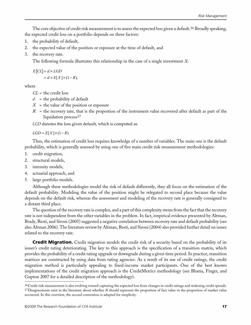
The core objective of credit risk measurement is to assess the expected loss given a default.16 Broadly speaking,the expected credit loss on a portfolio depends on three factors:

1. the probability of default,2. the expected value of the position or exposure at the time of default, and3. the recovery rate.

The following formula illustrates this relationship in the case of a single investment X:

where

CL = the credit lossd = the probability of defaultX = the value of the position or exposureR = the recovery rate, that is the proportion of the instrument value recovered after default as part of the

liquidation process17

LGD denotes the loss given default, which is computed as

Thus, the estimation of credit loss requires knowledge of a number of variables. The main one is the defaultprobability, which is generally assessed by using one of five main credit risk measurement methodologies:

1. credit migration,2. structural models,3. intensity models,4. actuarial approach, and5. large portfolio models.

Although these methodologies model the risk of default differently, they all focus on the estimation of thedefault probability. Modeling the value of the position might be relegated to second place because the valuedepends on the default risk, whereas the assessment and modeling of the recovery rate is generally consigned toa distant third place.

The question of the recovery rate is complex, and a part of this complexity stems from the fact that the recoveryrate is not independent from the other variables in the problem. In fact, empirical evidence presented by Altman,Brady, Resti, and Sironi (2005) suggested a negative correlation between recovery rate and default probability (seealso Altman 2006). The literature review by Altman, Resti, and Sironi (2004) also provided further detail on issuesrelated to the recovery rate.

Credit Migration. Credit migration models the credit risk of a security based on the probability of itsissuer’s credit rating deteriorating. The key to this approach is the specification of a transition matrix, whichprovides the probability of a credit rating upgrade or downgrade during a given time period. In practice, transitionmatrices are constructed by using data from rating agencies. As a result of its use of credit ratings, the creditmigration method is particularly appealing to fixed-income market participants. One of the best knownimplementations of the credit migration approach is the CreditMetrics methodology (see Bhatia, Finger, andGupton 2007 for a detailed description of the methodology).

16Credit risk measurement is also evolving toward capturing the expected loss from changes in credit ratings and widening credit spreads.17Disagreements exist in the literature about whether R should represent the proportion of face value or the proportion of market valuerecovered. In this overview, the second convention is adopted for simplicity.

E CL d LGD

d E X R

[ ] = ×= × × −[ ] ( ),1

LGD E X R= × −[ ] ( )1

Risk Management


The credit migration approach is not without problems. Rating agencies provide only historical data that canbe scarce in some sectors, such as sovereign issuers. In addition, the rating process differs among agencies, whichleads to the possibility of split ratings.18 Finally, these transition matrices are generally static and do not reflectthe relationship between the rating dynamics and the phases of the business cycle.

A body of research has been developed to address problems linked to the estimation of rating transitionmatrices. For example, Hu, Kiesel, and Perraudin (2002) developed a method to estimate the rating transitionmatrices for sovereign issuers. Jafry and Schuermann (2004) compared two common rating transition matrixestimation methods and proposed a new method to empirically evaluate the resulting matrices. In particular, theyshowed that the choice of the estimation method has a large effect on the matrix and thus on the amount ofeconomic capital required to support the portfolio.

Research has also been produced that deals with some issues created by the rating process, such as securitieswith split ratings. Split ratings may indicate a higher likelihood of an impending rating transition than othersecurities with homogenous ratings. Livingston, Naranjo, and Zhou (2008) considered this specific problem byinvestigating the link between split ratings and rating migration.

From a mathematical perspective, credit migration models use a probabilistic concept known as Markovchains.19 The Markov chains concept opens the door to a large number of computational techniques that arenecessary to build truly dynamic rating transition models and evaluate the risk of complex financial instruments,such as collateralized debt obligations. For example, Frydman and Schuermann (2008) proposed a rating transitionmodel based on a mixture of two Markov chains, and Kaniovski and Pflug (2007) developed a pricing and riskmanagement model for complex credit securities.

Structural Models. Structural models use such issuer-specific information as value of assets and liabilitiesto assess the probability of default. The best-known and most often used structural model is the contingent claimmodel derived from Robert Merton’s observation that a company’s equity can be viewed as a European optionwritten on the assets of the company, with an exercise price equal to the value of its debt and an expirationcorresponding to the maturity of the debt (see Merton 1974 and Geske 1977). Schematically, if the asset valueexceeds the debt value at the expiration date, then the option is in the money. Shareholders will exercise theiroption by paying the debt and regaining control of the company’s assets. On the contrary, if at the time the debtcomes due the value of the asset is less than the value of the debt, the option is out of the money. In this event,the shareholders have no incentive to exercise their option; they will let the option expire and default on the debt.Hence, based on Merton’s insight, the default probability is in some sense linked to the probability that the optionwill not be exercised. Although theoretically appealing, any implementation of this approach needs to overcomesignificant practical hurdles, which KMV addressed in developing a well-recognized contingent claim–basedmodel (see Kealhofer 2003a, 2003b).20

Other structural models exist. The first-passage approach, initially derived by Black and Cox (1976), wasclosely related to the contingent claim approach and has been popular in academic circles. In this methodology,the default time is modeled as the first time the asset value crosses below a given threshold. This analogy allowsthe default probability for a given time horizon to be found. Leland (1994) and Longstaff and Schwartz (1995)substantially generalized the first-passage approach. Zhou (2001), Collin-Dufresne and Goldstein (2001), andHilberink and Rogers (2002) subsequently extended it.

18A security is said to have a split rating when at least two of the rating agencies covering it assign different ratings.19Markov chains are a type of stochastic, or random, process that can take only a discrete number of values, or states. The key characteristicof Markov chains is that the transition probability between a current state A and a future state B depends exclusively on the current stateA. In fact, Markov chains do not have memory beyond the current state. 20KMV is now owned by Moodys. Stephen Kealhofer is one of the founders, along with John McQuown and Oldrich Vasicek.

Risk Management


Recently, Chen, Fabozzi, Pan, and Sverdlove (2006) empirically tested several structural models, includingthe Merton model and the Longstaff and Schwartz model. They found that making the assumption of randominterest rates and random recovery has an effect on the accuracy of the model, whereas assuming continuous defaultdoes not. They also observed that all structural models tested seem to have similar default prediction power.

Intensity Models. Intensity models, or reduced form models, originated in asset pricing theory and arestill mostly used for asset pricing purposes. In these models, analysts model the timing of the default as a randomvariable. This approach is self-contained because it is based neither on the characteristics of the company’s balancesheet nor on the structure of a rating model. It is consistent with current market conditions because the parametersused are generally inferred directly from market prices.

The simplest implementation is a binomial tree adapted for the possibility of default, but as thesophistication of intensity models increases so does the sophistication of the mathematical tools required. As aresult of their (relative) mathematical tractability, intensity-based models have been a very active research areanot only in terms of risk management but also in asset pricing, portfolio optimization, and even probabilitytheory. The manuscripts by Duffie and Singleton (2003) and Lando (2004) are among the nicest and mostaccessible references for intensity models.

Actuarial Approach. The actuarial approach uses techniques from actuarial sciences to model theoccurrence of default in large bond or loan portfolios. One of the best-known actuarial approaches is CreditRisk+(see Gundlach and Lehrbass 2004 for a detailed, although technical, look at CreditRisk+). To derive a probabilitydistribution for the credit loss of a portfolio, CreditRisk+ first models the frequency of defaults, assuming that theprobability distribution of the number of defaults in the portfolio follows a Poisson distribution. Credit Risk+then applies a loss given default to each default event. The parameters required in the analysis are estimated byusing historical statistical data.

Large Portfolio Models. Credit migration, structural models, and intensity models work very well forrelatively small portfolios. As the number of assets in the portfolio grows, however, the computational complexitytends to increase rapidly and the mathematical tractability declines quickly.

Vasicek (see Vasicek 1987, 1991, and 2002) extended the structural Merton model to value large loan portfolios.Allowing for default correlation between the various loans, Vasicek analyzed the asymptotic behavior of the Mertonvaluation model as the number of loans grew to infinity. To make computation simpler and more efficient, heassumed that the portfolio was homogeneous, in the sense that all the loans had the same parameters and samepairwise default correlation. The resulting model was tractable and provided a surprisingly good approximation forportfolios consisting of several dozen loans. This result is an undeniable advantage because traditional models tendto become mathematically and computationally intractable as the number of loans increases. In contrast, theaccuracy of the Vasicek large portfolio model improves with the number of loans in the portfolio.

Davis and Lo (2001) modeled counterparty risk in a large market as a credit contagion.21 Their model startedwith the simple idea that at the counterparty level, default may spread like the flu. If a financial entity caught theflu (defaults), then a chance exists that its counterparties could catch it as well. And if they do, they might infecttheir own counterparties.

Crowder, Davis, and Giampieri (2005) modeled default interaction by introducing a hidden state variablerepresenting a common factor for all of the bonds in the portfolio. This hidden Markov chains approach produceda tractable and computationally efficient dynamic credit risk model.

One of the common characteristics of all these large portfolio models is that they avoid developing a fulldefault correlation matrix. The default correlation matrix is notoriously difficult to estimate accurately, and its fastincreasing size is generally credited with the sharp rise in computational complexity.

21See Jorion and Zhang (2007) for a different view of credit contagion.

Risk Management


Operational RiskRegulatory frameworks, such as the Basel II Accord, have sparked an intense interest in the modeling of operationalrisk. A discussion of these regulatory requirements in the context of operational risk can be found in Embrechts,Frey, and McNeil (2005, ch. 10) or Chernobai, Rachev, and Fabozzi (2007, ch. 3).

Basel II rightfully acknowledges operational risk as a main source of financial risk. In fact, even if operationalrisk does not reach the disastrous levels observed in such downfalls as Barings or Daiwa, it may still take a heavytoll. Cummins, Lewis, and Wei (2006) analyzed the effect of operational loss on the market value of U.S. banksand insurance companies during the period of 1978 to 2003. They focused on the 403 banks and 89 insurers whosuffered operational losses of $10 million or more. They found that a statistically significant drop in their shareprice occurred and that the magnitude of this fall tended to be larger than that of the operational loss.

As can be expected, operational risk is more difficult to estimate than credit risk and far more difficult thanmarket risk. Similar to credit risk, the main obstacle in the application of risk measures to operational risk remainsthe generation of a probability distribution of operational loss. Most of the technical developments in themeasurement of operational risk have taken place in the past 10 years because increased awareness and regulatorypressures combined to propel operational risk to center stage.22

In their brief article, Smithson and Song (2004) examined a number of actuarial techniques and tools usedto evaluate operational risk. All the techniques have one common feature in that they attempt to circumventoperational risk’s greatest technical and analytical difficulty—the sparseness of available data. This relative lack ofdata is the result of several factors. To begin with, the existence of operational risk databases is quite recent.Moreover, occurrences of some of the operational risk, such as system failure, may be rare. Finally, industrywidedatabase sharing efforts are still in their infancy.

Among the techniques surveyed by Smithson and Song (2004), extreme value theory (EVT) deserves a specialmention. With its emphasis on the analysis and modeling of rare events and its roots in statistical and probabilistictheory, EVT constitutes an essential and very successful set of techniques for quantifying operational risk. As itsname indicates, EVT was originally designed to analyze rare events, or conversely to develop statistical estimateswhen only a few data points are reliable. Insurance companies exposed to natural disasters and other “catastrophes”have quickly adopted EVT. Embrechts, Klüppelberg, and Mikosch (2008) provided a thorough reference on EVTand its applications to finance and insurance, while Embrechts, Frey, and McNeil (2005, ch. 10) demonstrated theuse of EVT in the context of operational risk. Among recent research, Chavez-Demoulin, Embrechts, andNešlehová (2006) introduced useful statistical and probabilistic techniques to quantify operational risk. In particular,they discussed EVT and a number of dependence and interdependence modeling techniques. Chernobai, Rachev,and Fabozzi (2007) proposed a related, although slightly more probabilistic, treatment of operational risk, with aparticular emphasis on the Basel II requirements and a discussion of VaR for operational risk.

From a corporate finance perspective, Jarrow (2008) proposed to subdivide operational risk for banks into (1)the risk of a loss as a result of the firm’s operating technology and (2) the risk of a loss as a result of agency costs.Jarrow observed that contrary to market and credit risk, which are both external to the firm, operational risk isinternal to the firm. In his opinion, this key difference needs to be addressed in the design of estimation techniquesfor operational risk. Jarrow further suggested that current operational risk methodologies result in an upwardlybiased estimation of the capital required because they do not account for the bank’s net present value generatingprocess, which in his view, should at least cover the expected portion of operational risk.

22Although operational risk now has a scholarly journal dedicated to it, the Journal of Operational Risk only started publishing in early 2006.

Risk Management


Liquidity RiskThe modeling and management of liquidity risk has now moved to the forefront of the risk managementcommunity’s preoccupations, as can be seen in the Bank for International Settlements report on liquidity risk(Bank for International Settlements 2006) and in Goodhart’s (2008) analysis of banks’ liquidity managementduring the financial turmoil of the past few years.

Although few empirical studies have focused on the quantification of liquidity risk in general, a large body ofresearch has so far focused on liquidation risk, which is the risk that a firm in need of liquidating some of its assetsmay not realize their full value. Duffie and Ziegler (2003) investigated liquidation risk using a three-asset modelwith cash, a relatively liquid asset, and an illiquid asset. They showed that the approach of selling illiquid assetsfirst and keeping cash and liquid assets in reserve may generally be successful, but it may fail in instances whenasset returns and bid–ask spreads have fat tails. Engle, Ferstenberg, and Russel (2006) took the broader view ofanalyzing trade execution cost and linked this analysis with the calculation of what they called a liquidity value-at-risk measure. On the equity market, Li, Mooradian, and Zhang (2007) studied the time series of NYSEcommissions and found that equity commissions were correlated with illiquidity measures.

From a more general, albeit more theoretical perspective, Jarrow and Protter (2005) showed how to implementthe Çetin, Jarrow, and Protter (2004) model to compute liquidity risk using such measures as VaR. From a regulatoryperspective, Ku (2006) considered the notion of “acceptable investment” in the face of liquidity risk and introduceda liquidity risk model. Finally, Acerbi and Scandolo (2008) produced a theoretical work about the place of liquidityrisk within the class of coherent risk measures and defined a class of coherent portfolio risk measures.

A New Classification of Risk MeasuresIn the section “Popular Risk Measures for Practitioners,” a number of risk measures were defined—some fromthe well-established investment theory literature, some from the relatively new risk management literature, andsome from the investment industry’s intense interest in improving its own understanding and evaluation of risk.In this section, the goal is to ascertain the properties of various risk measures and define a more relevantclassification than the triptych of measures from investment theory, measures from risk management, and industry-driven measures that has been used so far.

A classification effort is needed because half a century of developments in the theory and practice of financehas produced a cornucopia of risk measures and raised a number of practical questions: Are all risk measures equally“good” at estimating risk? If they are, then should some criteria exist that desirable risk measures need to satisfy?Finally, should all market participants, traders, portfolio managers, and regulators use the same risk measures?

But these questions can only be answered after developing an understanding of the risk measurement processbecause understanding the measurement process helps develop important insights into specific aspects of the riskbeing measured. After all, a man with a scale in his hands is more likely to be measuring weights than distances. Inthe same spirit, understanding how risk is being measured by knowing the properties of the risk measures being usedwill help in understanding not only the dimensions of risk being captured but also the dimensions of risk left aside.

In this section, risk measures are classified as families or classes that satisfy sets of common properties. We willdiscuss four classes of risk measures and explore how the risk measures introduced earlier fit in this new classification:1. monetary risk measures,2. coherent risk measures,3. convex risk measures, and4. spectral risk measures.

Figure 10 summarizes the relationships between the classes and measures.

Risk Management


This classification system built on Artzner, Delbaen, Eber, and Heath’s (1997, 1999) highly influential workon coherent risk measures is not the only possible system.23 Indeed, at the time Artzner, Delbaen, Eber, andHeath were perfecting their system, Pedersen and Satchell (1998) proposed in the actuarial literature a similarclassification based on the nonnegativity, positive homogeneity, subadditivity, and translation invarianceproperties. In the insurance literature, Wang, Young, and Panjer (1997) also presented a system equivalent to theproperties of Artzner, Delbaen, Eber, and Heath. In the finance literature, Černý and Hodges (2000) introducedthe idea of “good deals.”

Monetary Risk Measures. Monetary risk measures, first introduced by Artzner, Delbaen, Eber, andHeath (1999), is a class of risk measures that equates the risk of an investment with the minimum amount of cash,or capital, that one needs to add to a specific risky investment to make its risk acceptable to the investor or regulator.In short, a monetary measure of risk ρ is defined as

where r represents an amount of cash or capital and X is the monetary profit and loss (P&L) of some investmentor portfolio during a given time horizon and is discounted back to the initial time.

What makes an investment “acceptable” will vary among investors and regulators. But this view of risk hasthe advantage of being simple, direct, and very much in line with some of the key questions asked by bank managersand regulators, clearinghouses, and OTC counterparties:• How much capital should a bank keep in reserve to face a given risk?• How much cash or collateral should be required of a clearinghouse member to cover the market value

fluctuations of the member’s positions?• How much collateral should be required from a counterparty to accept a trade?

Figure 10. Overview of Risk Measures

23The article by Artzner, Delbaen, Eber, and Heath (1997) is more finance oriented, whereas the more rigorous analysis found in Artzner,Delbaen, Eber, and Heath (1999) has a distinct mathematical orientation. We will refer to Artzner, Delbaen, Eber, and Heath (1999) orsimply Artzner, Delbaen, Eber, and Heath to indicate the entire body of work.

OmegaMeasure

StandardDeviation

σ

StandardDeviation

σVaR

ES, CVaR

ES, CVaR

(returndistribution) (discontinuous

distribution)

(continuousdistribution)

(P&Ldistribution)

(continuousdistribution)

WCE

Measures of Risk

Monetary Measure of Risk

Convex Measures of Risk

Coherent Measures of Risk

Spectral Measures of Risk

ρ( ) : minX X rr

= +( )≥0

an investment in a position is acceptablee⎡⎣ ⎤⎦ ,

Risk Management


Specific acceptability rules often are not mentioned. In that event, it is customary to assume that an investmentis deemed acceptable if it does not incur a loss. In this context, a monetary risk measure is a function of the absoluteloss that an investor could potentially incur on a position. Although this interpretation implies that these absoluterisk measures can be useful to assess the risk incurred by investment managers, it may not be the most appropriatein some cases. Two examples illustrate this point. First, to a manager of a fully funded pension fund, absolutelosses on the investment portfolio may be less relevant than a measure of risk on the surplus, which is the differencebetween the value of the investment portfolio and the actuarial value of the pension fund’s liability. Second, ahedge fund promising a given return target to its investors may be more interested in tracking the relative lossfrom the target rather than the absolute loss (from zero).

From the definition above, two important properties of monetary risk measures can be determined:• Risk can be expressed as a monetary amount in U.S. dollars, British pounds, euro, and so on.• The measure ρ(.) can be viewed as the “distance” between an investment’s potential loss and an acceptable

level of loss. For example, in the case of a 95 percent three-day VaR, the investment’s potential loss is a three-day loss with up to 95 percent confidence. Hence, any loss beyond the 95 percent confidence is not capturedin the VaR’s definition of potential loss.

Coherent Risk Measures. Acerbi (2007) provided an accessible overview of coherent risk measures andtheir practical applications. Artzner, Delbaen, Eber, and Heath (1999) defined coherent risk measures as the classof monetary risk measures satisfying the following four “coherence” properties:1. Monotonicity: If the return of asset X is always less than that of asset Y, then the risk of asset X must be

greater. This translates into24

2. Subadditivity: The risk of a portfolio of assets cannot be more than the sum of the risks of the individualpositions. Formally, if an investor has two positions in investments X and Y, then

This property guarantees that the risk of a portfolio cannot be more (and should generally be less) than thesum of the risks of its positions, and hence it can be viewed as an extension of the concept of diversificationintroduced by Markowitz. This property is particularly important for portfolio managers and banks trying toaggregate their risks among several trading desks.

3. Homogeneity: If a position in asset X is increased by some proportion k, then the risk of the position increasesby the same proportion k. Mathematically,

This property guarantees that risk scales according to the size of the positions taken. This property, however,does not reflect the increased liquidity risk that may arise when a position increases. For example, owning500,000 shares of company XYZ might be riskier than owning 100 shares because in the event of a crisis,selling 500,000 shares will be more difficult, costly, and require more time. As a remedy, Artzner, Delbaen,Eber, and Heath proposed to adjust X directly to reflect the increased liquidity risk of a larger position.

4. Translation invariance or risk-free condition: Adding cash to an existing position reduces the risk of theposition by an equivalent amount. For an investment with value X and an amount of cash r,

24As an alternative to this first property, one could consider positivity—if an investment makes a profit in every state of the world, thenits risk cannot be more than 0, that is X 0 ρ X( ) 0.≤⇒≥

X Y X Y≤ ⇒ ≥ in all states of the world ρ ρ( ) ( ).

ρ ρ ρ( ) ( ) ( ).X Y X Y+ ≤ +

ρ ρ( ) ( ).kX k X=

ρ ρ( ) ( ) .X r X r+ = −

Risk Management


Equipped with a definition of coherent risk measures, the following two questions can be addressed: Iscoherence necessary? And are the measures introduced earlier coherent?

Coherence is not necessary for all applications. Depending on whether one is a banker, portfolio manager, orregulator, some of the properties will be more important than others. The obvious example is subadditivity, whichis primordial in portfolio management applications. Another example would be translation invariance, whichunderpins the regulatory applications of a risk measure.

Regarding the second question, standard deviation calculated using a distribution of asset returns is not amonetary measure and, as a result, it cannot be coherent. Standard deviation calculated using a P&L distributionis a monetary measure, but it is not coherent because it does not satisfy the monotonicity property.

Value at risk is not coherent because it does not satisfy the subadditivity property. Artzner, Delbaen, Eber,and Heath formally demonstrated that VaR lacks the subadditivity property.25 This sharp contradiction with theprinciple of diversification should be of particular concern to a bank risk manager who aims at aggregating theVaR of various desks to obtain an overall VaR for the bank’s trading operations. Because the VaR fails to besubadditive, no assurance exists that the bank’s VaR will reflect the diversification occurring among desks.Daníelson, Embrechts, Goodhart, Keating, Muennich, Renault, and Shin (2001) further warned that thewidespread use of VaR, especially at the regulatory level, could result in a significant increase in systemic risk.Daníelson (2002) also criticized risk modeling in general and VaR in particular, pointing out the volatility of riskmeasures and the limited guidance they provide in times of crisis.

Expected shortfall was shown to be a coherent measure by Acerbi and Tasche (2002).For conditional value at risk, when the P&L distribution is continuous, CVaR and ES coincide, and as a

result CVaR is coherent. When the P&L distribution is not continuous, CVaR is not coherent. To remedy thisproblem, Rockafellar and Uryasev (2002) refined the definition of CVaR to ensure that it remains a coherentmeasure even for discontinuous distribution functions. To do so, they introduced a standardized α-tail cumulativedensity function, FX

α (.), defined as

which represents the cumulative distribution of conditional probabilities given that the investment value is in theα-tail (see Figure 11).

The CVaR (X;α) is then computed as the expected value of X in the α-tail:

The authors also introduced a lower and an upper bound for CVaR,

where CVaR− and CVaR+ are respectively defined as

and

25In fact, VaR is only subadditive when the investment value follows an elliptic distribution such as the normal or t-distribution. In this case,the VaR coincides with a 1-tailed confidence interval built using the standard deviation. See Embrechts, McNeil, and Straumann (2002).

F ( )

F ( )F ( )

F ( )

,X

XX

X

x

xx

x

α αα

α

=≤

>

⎧

⎨⎪⎪

⎩⎪⎪

if

if1

CVaR is in the -tail

( ; ) F .X xd xXx

α αα

= ( )∫

CVaR CVaR CVaR− +≤ ≤( ; ) ( ; ) ( ; ),X X Xα α α

CVaR− −= − < ( )⎡⎣⎢

⎤⎦⎥( ; ) | FX E X X

Xα α1

CVaR+ −= − ≤ ( )⎡⎣⎢

⎤⎦⎥( ; ) | F .X E X X

Xα α1

Risk Management


When the distribution is continuous, the CVaR will coincide with its upper and lower bounds and with theexpected shortfall. That is26

Extensions to the Definition of Coherent Risk Measures. Log coherence, coherent utilityfunctions, coherence and general equilibrium, and multiperiod coherent risk measures are extensions to thedefinition of coherent risk measures.

■ Log coherence: Bielecki and Pliska (2003) extended the coherence framework by introducing a set of log-coherence properties that can be applied to measure of risks based on the distribution of instantaneous (log) returns.

■ Coherent utility functions: Cherny and Madan (2006) introduced the concept of coherent utility functionsas a complement to coherent risk measures. They also pointed out that risk-adjusted performance measures, p(.),can be defined out of any coherent risk measure, ρ(.), using the following definition:

where λ represents the investor’s risk aversion. In fact, p(.) is also a utility function according to the Cherny andMadan concept.

Figure 11. CDF and Standardized �-Tail CDF

26An interesting notion arises with the choice α = 1. In this case, the CVaR and expected shortfall coincide with the expected profit orloss of investment X, that is CVaR(X;1) = ES(X;1) = E [X]. Hence, the expected P&L of a position can be viewed as one of the simplestpossible coherent risk measure.

XmaxXmin


A. Cumulative Density Function

1

α0


B. Standardized α-Tail Cumulative Density Function

1

0XmaxXmin

α-Tail of the Distribution

CVaR CVaR CVaR ES− += = =( ; ) ( ; ) ( ; ) ( ; ).X X X Xα α α α

p X E X X( ) ( ),= [ ]− λρ

Risk Management


■ Coherence and general equilibrium: Csóka, Herings, and Kóczy (2007) explored the coherence propertiesfrom a general equilibrium perspective.

■ Multiperiod coherent risk measures: Artzner, Delbaen, Eber, Heath, and Ku (2007) proposed a multiperiodmeasurement process for coherent risk measures.

Convex Risk Measures. Convex risk measures are an active and quite technical area of risk managementresearch, with contributions by Föllmer and Schied (2002a, 2002b) and more recently by Ben-Tal and Teboulle(2007), Klöppel and Schweizer (2007), as well as Jobert and Rogers (2008).

Föllmer and Schied (2002a) introduced the concept of convex risk measure by noting that the risk of someinstruments may not increase linearly with the size of the position. This contradicts the homogeneity propertiesof Artzner et al. They thus proposed to relax the homogeneity and subadditivity properties and replace themwith convexity.

The risk measure of a portfolio with two positions in investments X and Y is a convex function if

As a result of loosening the original properties of coherence, any coherent risk measure is necessarily convex,whereas convex risk measures are not necessarily coherent. Szegö (2002) also pointed out that as a result of itslack of subadditivity, VaR is neither coherent nor convex. Indeed, embedded in the convexity property is thesubadditivity property. Hence, diversification is properly rewarded by using convex risk measures.

Spectral Risk Measures. Kusuoka (2001) and Acerbi (2002) independently introduced the class ofspectral risk measures, which are coherent risk measures that can be parameterized by means of a risk-aversionfunction. The clear advantage of spectral risk measures is that, contrary to the expected shortfall or CVaR-typeof measures, they can take into account the entire return distribution rather than just the left tail. In fact, it turnsout that expected shortfall (and thus CVaR when the return distribution is continuous) is a prominent andparticularly simple member of this class of risk measures, in which the risk aversion function is constant on theinterval (0,α).

Moreover, Tasche (2002) showed that not only can expected shortfall be represented as an average of valueat risk computed on a continuum of confidence levels but that a similar representation exists for all spectralmeasures. He also demonstrated that spectral risk measures are the subclass of coherent risk measures that, inaddition to satisfying the four coherence properties, satisfy the following two properties:• Law invariance: If X and Y have the same probability distribution (otherwise known as the probability law),

then they will have the same risk:

• Commonotonic additivity: With two (nondecreasing) functions, f and g, the risk of investment Z, whereZ = f (X) + g(Y), is simply the sum of the risks of investments A and B, where A = f(X) and B = g(X). So,the risk of a sum of functions of a given investment is the sum of the risks:

Cherny and Madan (2006) introduced two new spectral risk measures: a two-parameter beta-VaR measure,whose name reveals the role played by the beta probability distribution in its definition, and a one parameteralpha-VaR measure, which is a restriction of the beta-VaR measure.

Acerbi and Simonetti (2002) applied spectral risk measures to portfolio selection by extending theoptimization method introduced for CVaR by Pflug (2000) and Rockafellar and Uryasev (2000). They alsoestablished a connection between the portfolio selection problem they considered and the mean–varianceoptimization of Markowitz (1952).

ρ λ λ λρ λ ρ λ( ) ( ) ( ), .X Y X Y+ −( ) ≤ + −( ) ≤ ≤1 1 0 1

P X u P Y u u X Y[ ] [ ] .≤ = ≤ ⇒ ( ) = ( ) for all possible values of ρ ρ

ρ ρ ρf( ) g( ) f( ) g( ) .X X X X+( ) = ( ) + ( )

Risk Management


Adam, Houkari, and Laurent (2007) conducted an empirical analysis of risk measure–based portfolio selectionusing a database of hedge fund returns. Their main finding is that although risk measures concentrated on thetail tend to promote higher portfolio diversification, risk measures focusing on the worst case scenario generallyseem to reduce portfolio diversification.

Take Away: So How Does All this Fit Together? Exhibit 2 illustrates the relationships amongthe risk measures discussed in this review, their origin, and the various classes they belong to.

The Quest for an Integrated Risk MeasurementRisk management is a continuously improving process. Although the practice of risk management is about improvingdecision making and control structure to make the firm management more dynamic, flexible, and enterprising, aswell as reduce the potential for “disasters” to occur, the science of risk measurement is constantly in search of moreaccurate risk measures, more efficient estimation methods, and new ways of quantifying the various dimensions ofrisk. Firms need to do more, however, than just compute each risk accurately and instantaneously. To control itsrisk-taking, a firm needs to set a risk budget and effectively allocate this budget to the firm’s various divisions. Thisrequirement assumes that the firm can aggregate all the types of risks it is exposed to into one consistent framework.

Asset managers have long used the traditional portfolio–based modern portfolio theory developed byMarkowitz, Sharpe, Treynor, Lintner, and Mosin in their risk management endeavors. In this “top-down”approach, the fundamental measure of risk is total risk (or in modern terms, “integrated risk”) embodied by thevariance of asset returns. Total risk can then be split into systematic risk (beta) and unsystematic risk as in singlefactor models, or divided even more finely into factor risks and unsystematic risk, as in multifactor models. Thistop-down view has given rise to numerous risk allocation applications, such as Grinold and Kahn (1999) and,more recently, Litterman (2008). But a notion of the amount of capital required to sustain an operation is missing,which is not surprising because this framework was developed with portfolios in mind; the capital is the wealthor equity ventured in the portfolio.

Financial institutions are relying on the modern discipline of risk measurement in their quest for an integratedrisk measurement framework. From its origin in the trading and lending world of banking, risk measurementdeveloped as a “bottom-up” approach articulated around risk factors and subfactors at the trading desk level. First,equity, interest rates, currency, and commodity market risk were considered, estimated using VaR and othermeasures, and aggregated into one market risk number. Next, credit risk was added, and operational risk andliquidity risk were considered as well. Central to this view is the idea that a bank’s capital is a scarce resource thatmust be deployed with care and only to activities with good risk-adjusted return potential. But such a capitalallocation or risk budgeting exercise can only be done effectively if all the risks measured at the desk level can bemeaningfully aggregated together. Numerous efforts to do that have already been undertaken, although no singleintegration methodology has yet emerged as predominant. To name a few, Jorion (2007) and Dowd (1998)designed VaR-based integrated risk measurement frameworks. Duffie and Singleton (2003) provided a high-leveloverview of the issues that need to be considered when integrating market and credit risk. Medova and Smith(2005) and Jobst, Gautam, and Zenios (2006) presented measurement frameworks integrating the market andcredit risk dimensions.

Exhibit 2. Classification of Some Popular Risk Measures

Origin Risk Measure Monetary Convex Coherent Spectral

Investment theory Variance and standard deviation (return distribution) No No No NoVariance and standard deviation (P&L distribution) Yes Yes No No

Modern risk management Value at risk Yes No No NoExpected shortfall Yes Yes Yes YesConditional value at risk Yes Yes Possibly PossiblyWorst case expectation Yes Yes Possibly Possibly

Street measure Omega No No No No

Risk Management


In attempts to answer the fundamental risk-budgeting question, traditional portfolio–based modern portfoliotheory and the modern discipline of risk measurement have started to converge. The blurring of cultures betweenasset managers and investment bankers has also contributed to strengthening and accelerating this trend.

ConclusionThe past 15 years have marked a true revolution in risk management. The science of risk measurement, once arelatively small topic in investment theory, has grown as a field of research in its own right. New risk measureshave been proposed and their properties studied. Because of the development of new analytical techniques,measures that in the past applied only to market risk have now found applications in credit, operational, andliquidity risk and also in portfolio optimization. In addition, a growing emphasis on risk budgeting has also sparkeda quest for an integrated risk measurement framework. Fundamentally, the tremendous success of theseinnovations is the result of a joint effort of the entire financial community: academics, practitioners, and regulators.

The practice of risk management has also matured considerably. But although the science of risk measurementhas advanced through the rationality of quantitative analysis, the practice of risk management has grown throughthe pains inflicted by the long list of financial disasters. Although often uneasy, learning from financial disastersis critical to the advancement of risk management. Indeed, disasters are a powerful reminder that good riskmeasurement is necessary but insufficient in ensuring good risk management.

Risk management is, therefore, not just a technical challenge that requires the attention of a few highly trainedquantitative analysts, but it is an organizational challenge in which everyone must participate. And at its base,good risk management needs to be rooted not only in appropriate controls but also in a strong personal andorganizational sense of ethics.

Risk Management


References

Acerbi, Carlo. 2002. “Spectral Measures of Risk: A Coherent Representation of Subjective Risk Aversion.” Journalof Banking & Finance, vol. 26, no. 7 ( July):1505-1518.

“We study a space of coherent risk measures Mϕ obtained as certain expansions of coherent elementarybasis measures. In this space, the concept of ‘risk aversion function’ ϕ naturally arises as the spectralrepresentation of each risk measure in a space of functions of confidence level probabilities. We givenecessary and sufficient conditions on ϕ for Mϕ to be a coherent measure. We find in this way a simpleinterpretation of the concept of coherence and a way to map any rational investor’s subjective riskaversion onto a coherent measure and vice-versa. We also provide for these measures their discreteversions M(N)ϕ acting on finite sets of N independent realizations of a r.v. which are not only shownto be coherent measures for any fixed N, but also consistent estimators of Mϕ for large N.” (p. 1505)

———. 2007. “Coherent Measures of Risk in Everyday Market Practice.” Quantitative Finance, vol. 7, no. 4(August):359–364.

“This article is a guided tour of the recent (sometimes very technical) literature on coherent riskmeasures (CRMs). Our purpose is to review the theory of CRMs from the perspective of practicalrisk management applications. We have tried to single out those results from the theory which helpto understand which CRMs can today be considered as realistic candidate alternatives to Value at Risk(VaR) in financial risk management practice.” (p. 359)

Acerbi, Carlo, and Giacomo Scandolo. 2008. “Liquidity Risk Theory and Coherent Measures of Risk.”Quantitative Finance, vol. 8, no. 7 (October):681–692.

“We discuss liquidity risk from a pure risk–theoretical point of view in the axiomatic context ofCoherent Measures of Risk. We propose a formalism for Liquidity Risk which is compatible with theaxioms of coherency. We emphasize the difference between ‘coherent risk measures’ (CRM) ρ(X)defined on portfolio values X as opposed to ‘coherent portfolio risk measures’ (CPRM) ρ(p) definedon the vector space of portfolios p, and we observe that in the the presence of liquidity risk the valuefunction on the space of portfolios is no more necessarily linear. We propose a new nonlinear ‘Value’function VL(p) which depends on a new notion of ‘liquidity policy’ L. The function VL(p) naturallyarises from a general description of the impact that the microstructure of illiquid markets has whenmarking a portfolio to market. We discuss the consequences of the introduction of the function VL(p)in the coherency axioms and we study the properties induced on CPRMs. We show in particular thatCPRMs are convex, finding a result that was proposed as a new axiom in the literature of so called‘convex measures of risk’. The framework we propose is not a model but rather a new formalism, inthe sense that it is completely free from hypotheses on the dynamics of the market. We provideinterpretation and characterization of the formalism as well as some stylized examples.” (p. 681)

Acerbi, Carlo, and Prospero Simonetti. 2002. “Portfolio Optimization with Spectral Measures of Risk.” Workingpaper (www.gloriamundi.org/detailpopup.asp?SubCatLev1ID=Portfolio+Optimization&ID=453054773).

“We study Spectral Measures of Risk from the perspective of portfolio optimization. We derive exactresults which extend to general Spectral Measures the Pflug–Rockafellar–Uryasev methodology forthe minimization of alpha—Expected Shortfall. The minimization problem of a spectral measure is

Risk Management


shown to be equivalent to the minimization of a suitable function which contains additionalparameters, but displays analytical properties (piecewise linearity and convexity in all arguments,absence of sorting subroutines) which allow for efficient minimization procedures. In doing so we alsoreveal a new picture where the classical risk–reward problem `a la Markowitz (minimizing risks withconstrained returns or maximizing returns with constrained risks) is shown to coincide to theunconstrained optimization of a single suitable spectral measure. In other words, minimizing a spectralmeasure turns out to be already an optimization process itself, where risk minimization and returnsmaximization cannot be disentangled from each other.” (p. 1)

Acerbi, Carlo, and Dirk Tasche. 2002. “On the Coherence of Expected Shortfall.” Journal of Banking & Finance,vol. 26, no. 7 ( July):1487–1503.

“Expected shortfall (ES) in several variants has been proposed as remedy for the deficiencies of value-at-risk (VaR) which in general is not a coherent risk measure. In fact, most definitions of ES lead tothe same results when applied to continuous loss distributions. Differences may appear when theunderlying loss distributions have discontinuities. In this case even the coherence property of ES canget lost unless one took care of the details in its definition. We compare some of the definitions ofES, pointing out that there is one which is robust in the sense of yielding a coherent risk measureregardless of the underlying distributions. Moreover, this ES can be estimated effectively even in caseswhere the usual estimators for VaR fail.” (p. 1487)

Adam, Alexander, Mohammed Houkari, and Jean-Paul Laurent. 2007. “Spectral Risk Measures and PortfolioSelection.” Working paper (http://laurent.jeanpaul.free.fr/Spectral_risk_measures_and_portfolio_selection.pdf ).

“This paper deals with risk measurement and portfolio optimization under risk constraints. Firstly wegive an overview of risk assessment from the viewpoint of risk theory, focusing on moment-based,distortion and spectral risk measures. We subsequently apply these ideas to an asset managementframework using a database of hedge funds returns chosen for their non-Gaussian features. We dealwith the problem of portfolio optimization under risk constraints and lead a comparative analysis ofefficient portfolios. We show some robustness of optimal portfolios with respect to the choice of riskmeasure. Unsurprisingly, risk measures that emphasize large losses lead to slightly more diversifiedportfolios. However, risk measures that account primarily for worst case scenarios overweight fundswith smaller tails which mitigates the relevance of diversification.” (p. 1)

Albanese, Claudio. 1997. “Credit Exposure, Diversification Risk and Coherent VaR.” Working paper,Department of Mathematics, University of Toronto (September).

This article is a precursor to Albanese and Lawi (2003). The author discusses the application of riskmeasures to credit portfolios. One of the most striking conclusions of this analysis is that the value-at-risk (VaR) measure fails to be subadditive because the VaR of an investment in a single credit-risky bondmay be larger than the VaR of a portfolio of credit-risky bonds issued by different entities. Albanese andLawi (2003) not only reiterate this analysis but update it to include a discussion of spectral risk measures.

Albanese, Claudio, and Stephan Lawi. 2003. “Spectral Risk Measures for Portfolios.” Working paper(www.level3finance.com/coherence.pdf ).

“In this article, we experiment with several different risk measures such as standard deviation, value-at-risk, expected shortfall and power-law spectral measures. We consider several families of test portfolios,one with a typical market risk profit-and-loss profile, and the others containing defaultable bonds ofvarious credit ratings and various degree of diversification. We find that the risk measures are roughlyequivalent on the market risk portfolios but differ significantly on the credit ones. In fact, value-at-riskas well as some coherent risk measures including expected shortfall have counter-intuitive features as afunction of the degree of diversification for return distributions deviating substantially from the normal.Certain spectral risk measures possess the most intuitive properties regarding diversification.” (p. 1)

Risk Management


Albrecht, Peter. 2004. “Risk Measures.” In Encyclopaedia of Actuarial Science. Hoboken, NJ: John Wiley & Sons.In this entry, Albrecht presents a brief overview of risk measures, including coherent risk measures,mostly from an actuarial perspective.

Altman, Edward. 2006. “Credit Risk, Corporate Defaults, and the Link between Default and Recovery Rates.”CFA Institute Conference Proceedings Quarterly, vol. 23, no. 3 (September):34–43.

“The U.S. high-yield bond market has grown dramatically in the past three decades, reaching morethan $1 trillion in outstanding debt as of mid-year 2006. But little rigorous analysis has been done onwhat happens to the recovery rate over the credit cycle. Most models assume a fixed recovery rate, buta recent model that was tested using more than 1,000 defaulted bonds shows an inverse relationshipbetween the probability of default and the recovery rate. Based on this model, several industries maybe quite vulnerable to a high risk of default in the current environment.” (p. 34)

Altman, Edward, Andrea Resti, and Andrea Sironi. 2004. “Default Recovery Rates in Credit Risk Modeling: AReview of the Literature and Empirical Evidence.” Economic Notes, vol. 2, no. 2 ( July):183–208.

“Evidence from many countries in recent years suggests that collateral values and recovery rates (RRs)on corporate defaults can be volatile and, moreover, that they tend to go down just when the numberof defaults goes up in economic downturns. This link between RRs and default rates has traditionallybeen neglected by credit risk models, as most of them focused on default risk and adopted static lossassumptions, treating the RR either as a constant parameter or as a stochastic variable independentfrom the probability of default (PD). This traditional focus on default analysis has been partly reversedby the recent significant increase in the number of studies dedicated to the subject of recovery rateestimation and the relationship between default and RRs. This paper presents a detailed review of theway credit risk models, developed during the last 30 years, treat the RR and, more specifically, itsrelationship with the PD of an obligor. Recent empirical evidence concerning this issue is alsopresented and discussed.” (p. 183)

Altman, Edward, Brooks Brady, Andrea Resti, and Andrea Sironi. 2005. “The Link between Default and RecoveryRates: Theory, Empirical Evidence and Implications.” Journal of Business, vol. 78, no. 6 (November):2203–2227.

“This paper analyzes the association between default and recovery rates on credit assets and seeks toempirically explain this critical relationship. We examine recovery rates on corporate bond defaultsover the period 1982–2002. Our econometric univariate and multivariate models explain a significantportion of the variance in bond recovery rates aggregated across seniority and collateral levels. We findthat recovery rates are a function of supply and demand for the securities, with default rates playinga pivotal role. Our results have important implications for credit risk models and for the procyclicalityeffects of the New Basel Capital Accord.” (p. 2203)

Artzner, Philippe, Freddy Delbaen, Jean-Marc Eber, and David Heath. 1997. “Thinking Coherently.” Risk,vol. 10 (November):68–71.

This short article contains Artzner, Delbaen, Eber, and Heath’s original discussion of the coherenceproperties of risk measures. When compared with Artzner et al. (1999), this article is often regardedas less mathematical and more finance oriented.

———. 1999. “Coherent Measures of Risk.” Mathematical Finance, vol. 9, no. 3 ( July):203–228.“In this paper we study both market risks and nonmarket risks, without complete markets assumption,and discuss methods of measurement of these risks. We present and justify a set of four desirableproperties for measures of risk, and call the measures satisfying these properties ‘coherent.’ We examinethe measures of risk provided and the related actions required by SPAN, by the SEC/NASD rules,and by quantile-based methods. We demonstrate the universality of scenario-based methods forproviding coherent measures. We offer suggestions concerning the SEC method. We also suggest amethod to repair the failure of subadditivity of quantile-based methods.” (p. 203)

Risk Management


Artzner, Philippe, Freddy Delbaen, Jean-Marc Eber, David Heath, and Hyejin Ku. 2007. “Coherent MultiperiodRisk Adjusted Values and Bellman’s Principle.” Annals of Operations Research, vol. 152, no. 1 ( July):5–22.

“Starting with a time-0 coherent risk measure defined for ‘value processes’, we also define riskmeasurement processes. Two other constructions of measurement processes are given in terms of setsof test probabilities. These latter constructions are identical and are related to the former constructionwhen the sets fulfill a stability condition also met in multiperiod treatment of ambiguity as in decision-making. We finally deduce risk measurements for the final value of locked-in positions and repeat awarning concerning Tail-Value-at-Risk.” (p. 5)

Bank for International Settlements. 2006. “The Management of Liquidity Risk in Financial Groups.” (2 May). In this report, the Joint Forum’s Working Group on Risk Assessment and Capital presents the resultsof a review of current liquidity risk management practices at large financial groups.

Basel Committee on Banking Supervision. 2004. “International Convergence of Capital Measurement andCapital Standards.” Bank for International Settlements ( June).

“This report presents the outcome of the Basel Committee on Banking Supervision’s (‘the Commit-tee’) work in recent years to secure international convergence on revisions to supervisory regulationsgoverning the capital adequacy of internationally active banks. Following the publication of theCommittee’s first round of proposals for revising the capital adequacy framework in June 1999, anextensive consultative process was set in motion in all member countries and the proposals were alsocirculated to supervisory authorities worldwide. The Committee subsequently released additionalproposals for consultation in January 2001 and April 2003 and conducted three quantitative effectstudies related to its proposals. As a result of these efforts, many valuable improvements have beenmade to the original proposals. The present paper is now a statement of the Committee and agreedto by all its members. It sets out the details of the agreed framework for measuring capital adequacyand the minimum standard to be achieved that the national supervisory authorities represented onthe Committee will propose for adoption in their respective countries. This framework and thestandards it contains have been endorsed by the Central Bank Governors and Heads of BankingSupervision of the G-10 countries.” (p. 1)

Ben-Tal, Aharon, and Marc Teboulle. 2007. “An Old-New Concept of Risk Measures: The Optimized CertaintyEquivalent.” Mathematical Finance, vol. 17, no. 3 ( July):449–476.

“The optimized certainty equivalent (OCE) is a decision theoretic criterion based on a utility function,that was first introduced by the authors in 1986. This paper re-examines this fundamental concept,studies and extends its main properties, and puts it in perspective to recent concepts of risk measures.We show that the negative of the OCE naturally provides a wide family of risk measures that fits theaxiomatic formalism of convex risk measures. Duality theory is used to reveal the link between theOCE and the ϕ-divergence functional (a generalization of relative entropy), and allows for derivingvarious variational formulas for risk measures. Within this interpretation of the OCE, we prove thatseveral risk measures recently analyzed and proposed in the literature (e.g., conditional value of risk,bounded shortfall risk) can be derived as special cases of the OCE by using particular utility functions.We further study the relations between the OCE and other certainty equivalents, providing generalconditions under which these can be viewed as coherent/convex risk measures. Throughout the paperseveral examples illustrate the flexibility and adequacy of the OCE for building risk measures.” (p. 449)

Bernstein, Peter. 1998. Against the Gods: The Remarkable Story of Risk. Hoboken, NJ: John Wiley & Sons.In this wonderfully written volume, Bernstein tells the tale of the concept of risk through the ages,from antiquity through to modern days. He demonstrates how the emergence of risk as an idea waspossible through not only the sophistication of mathematical theories and techniques but also aprofound social and philosophical evolution. Bernstein narrates the story of risk using the lives of themain protagonists in its development, including Cardano, Pascal, and Fermat, von Neumann andMorgenstern, and Amos and Tversky.

Risk Management


———. 2006. “Risk: The Hottest Four-Letter Word in Financial Markets.” CFA Institute Conference ProceedingsQuarterly, vol. 23, no. 3 (September):10–15.

“The future is uncertain, so we can never know what will happen. Indeed, risk would not exist if we couldcorrectly anticipate the future. But rather than reacting blindly to adverse—or even favorable—events,investors can prepare themselves for the future by imagining plausible outcomes. As opposed to thenotion that risk management is only about the calculation of probabilities, I assert that risk managementis quality decision making in the face of uncertainty. Thus, investors must live with the inevitability thattheir decisions will sometimes be wrong.” (p. 10)

Bertsimas, Dimitris, Geoffrey Lauprete, and Alexander Samarov. 2004. “Shortfall as a Risk Measure: Properties,Optimization and Applications.” Journal of Economic Dynamics & Control, vol. 28, no. 7 (April):1353–1381.

“Motivated from second-order stochastic dominance, we introduce a risk measure that we callshortfall. We examine shortfall’s properties and discuss its relation to such commonly used riskmeasures as standard deviation, VaR, lower partial moments, and coherent risk measures. We showthat the mean-shortfall optimization problem, unlike mean-VaR, can be solved efficiently as a convexoptimization problem, while the sample mean-shortfall portfolio optimization problem can be solvedvery efficiently as a linear optimization problem. We provide empirical evidence (a) in asset allocation,and (b) in a problem of tracking an index using only a limited number of assets that the mean-shortfallapproach might have advantages over mean-variance.” (p. 1353)

Bhatia, Mickey, Christopher Finger, and Greg Gupton. 2007. “CreditMetrics Technical Document.” RiskMetricsGroup (www.riskmetrics.com).

“The reference document for CreditMetrics, it is meant to serve as an introduction to the methodologyand mathematics behind statistical credit risk estimation, as well as a detailed documentation of theanalytics that generate the data set provided. This document reviews:• the conceptual framework of our methodologies for estimating credit risk;• the description of the obligors’ credit quality characteristics, their statistical description and

associated statistical models;• the description of credit exposure types across ‘market-driven’ instruments and• the more traditional corporate finance credit products; and• the data set that we update periodically and provide to the market for free.” (p. 1)

Bielecki, Tomasz, and Stanley Pliska. 2003. “Economic Properties of the Risk Sensitive Criterion for PortfolioManagement.” Review of Accounting and Finance, vol. 2, no. 2:3–17.

“The idea of using stochastic control methods for theoretical studies of portfolio management haslong been standard, with maximum expected utility criteria commonly being used. But in recent yearsa new kind of criterion, the risk sensitive criterion, has emerged from the control theory literature andbeen applied to portfolio management. This paper studies various economic properties of this criterionfor portfolio management, thereby providing justification for its theoretical and practical use. Inparticular, it is shown that the risk sensitive criterion amounts to maximizing a portfolio’s risk adjustedgrowth rate. In other words, it is essentially the same as what is commonly done in practice: find thebest trade-off between a portfolio’s average return and its average volatility.” (p. 3)

Black, Fisher, and John Cox. 1976. “Valuing Corporate Securities: Some Effects of Bond Indenture Provisions.”Journal of Finance, vol. 31, no. 2 (May):351–367.

“Our objective in this paper is to make some general statements on this valuation process and thenturn to an analysis of a certain type of bond indenture provisions which are often found in practice.Specifically, we will look at the safety covenants, subordination arrangements, and restrictions on thefinancing of interest and dividend payments.” (p. 351)

Risk Management


Černý, Ales, and Stewart Hodges. 2000. “The Theory of Good-Deal Pricing in Financial Markets.” ResearchReport. FORC Preprint No. 98/90, Cass Business School, London.

“In this paper, the term ‘good-deal pricing’ stands for any pricing technique based on the absence ofattractive investment opportunities—good deals—in equilibrium. The theory presented indicates thatany such technique can be seen as a generalization of no-arbitrage pricing and that, with a little bitof care, it will contain the no-arbitrage and the representative agent equilibrium as the two oppositeends of a spectrum of possible no-good-deal equilibrium restrictions. We formulate the Extensionand the Pricing Theorem in no-good-deal framework and establish general properties of no-good-deal price bounds determined by von Neumann-Morgenstern preferences.” (p. 1)

Çetin, Umut, Robert Jarrow, and Philip Protter. 2004. “Liquidity Risk and Arbitrage Pricing Theory.” Financeand Stochastics, vol. 8, no. 3 (August):311–341.

“Classical theories of financial markets assume an infinitely liquid market and that all traders act asprice takers. This theory is a good approximation for highly liquid stocks, although even there it doesnot apply well for large traders or for modelling transaction costs. We extend the classical approachby formulating a new model that takes into account illiquidities. Our approach hypothesizes astochastic supply curve for a security’s price as a function of trade size. This leads to a new definitionof a self-financing trading strategy, additional restrictions on hedging strategies, and some interestingmathematical issues.” (p. 311)

Chavez-Demoulin, Valerie, Paul Embrechts, and Johanna Nešlehová. 2006. “Quantitative Models for OperationalRisk: Extremes, Dependence and Aggregation.” Journal of Banking & Finance, vol. 30, no. 10 (October):2635–2658.

“Due to the new regulatory guidelines known as Basel II for banking and Solvency 2 for insurance,the financial industry is looking for qualitative approaches to and quantitative models for operationalrisk. Whereas a full quantitative approach may never be achieved, in this paper we present sometechniques from probability and statistics which no doubt will prove useful in any quantitativemodelling environment. The techniques discussed are advanced peaks over threshold modelling, theconstruction of dependent loss processes and the establishment of bounds for risk measures underpartial information, and can be applied to other areas of quantitative risk management.” (p. 2635)

Chen, Ren-Raw, Frank J. Fabozzi, Ging-Ging Pan, and Ronald Sverdlove. 2006. “Sources of Credit Risk:Evidence from Credit Default Swaps.” Journal of Fixed Income (Winter):7–21.

The authors test empirically several structural models, including the Merton model, the Longstaffand Schartz model, and the Rabinovitch model, using credit default swaps data. They find that makingthe assumption of random interest rates and random recovery has an important effect, whereasassuming continuous default does not. They also observe that all structural models tested seem to havesimilar predictive accuracy.

Chernobai, Anna, Svetlozar Rachev, and Frank Fabozzi. 2007. Operational Risk: A Guide to Basel II CapitalRequirements, Models, and Analysis. Hoboken, NJ: John Wiley & Sons.

The authors define operational risk in relation to other types of risk and detail the operational riskrequirements related to the Basel II Accord. They also present an array of probabilistic methods usedto model operational risk and show how to compute VaR for operational risk.

Cherny, Alexander, and Dilip Madan. 2006. “Coherent Measurement of Factor Risks.” Working paper (http://papers.ssrn.com/sol3/papers.cfm?abstract_id=904543#PaperDownload).

“We propose a new procedure for the risk measurement of large portfolios. It employs the followingobjects as the building blocks: — coherent risk measures introduced by Artzner, Delbaen, Eber, and Heath; — factor risk measures introduced in this paper, which assess the risks driven by particular factors

like the price of oil, S&P500 index, or the credit spread; — risk contributions factor risk contributions, which provide a coherent alternative to the

sensitivity coefficients.

Risk Management


We also propose two particular classes of coherent risk measures called Alpha VAR and Beta VAR,for which all the objects described above admit an extremely simple empirical estimation procedure.This procedure uses no model assumptions on the structure of the price evolution.

Moreover, we consider the problem of the risk management on a firm’s level. It is shown that if therisk limits are imposed on the risk contributions of the desks to the overall risk of the firm (ratherthan on their outstanding risks) and the desks are allowed to trade these limits within a firm, then thedesks automatically find the globally optimal portfolio.” (p. 1)

Collin-Dufresne, Pierre, and Robert Goldstein. 2001. “Do Credit Spreads Reflect Stationary Leverage Ratios?”Journal of Finance, vol. 56, no. 5 (October):1929–1957.

“Classical theories of financial markets assume an infinitely liquid market and that all traders act asprice takers. This theory is a good approximation for highly liquid stocks, although even there it doesnot apply well for large traders or for modelling transaction costs. We extend the classical approachby formulating a new model that takes into account illiquidities. Our approach hypothesizes astochastic supply curve for a security’s price as a function of trade size. This leads to a new definitionof a self-financing trading strategy, additional restrictions on hedging strategies, and some interestingmathematical issues.” (p. 1929)

Crouhy, Michel, Dan Galai, and Robert Mark. 2001. Risk Management. New York: McGraw-Hill Professional.

The authors present a highly accessible, yet detailed, overview of the practice and concepts of riskmanagement from a banking perspective. They cover the various types of risk as well as estimationmethods and provide an overview of the regulatory environment. Particular emphasis is giventhroughout to credit risk modeling.

———. 2006. The Essentials of Risk Management. New York: McGraw-Hill Professional.

The authors provide a higher level and less technical overview of risk management than Crouhy,Galai, and Mark (2001). The range of topics covered in this volume is broadly similar to that of thelatter, although Crouhy, Galai, and Mark (2006) covers corporate risk management and accentuatesless the regulatory aspects inherent in banking risk management.

Crowder, Martin, Mark Davis, and Giacomo Giampieri. 2005. “Analysis of Default Data Using Hidden MarkovModels.” Quantitative Finance, vol. 5, no. 1 (February):27–34.

“The occurrence of defaults within a bond portfolio is modelled as a simple hidden Markov process.The hidden variable represents the risk state, which is assumed to be common to all bonds within oneparticular sector and region. After describing the model and recalling the basic properties of hiddenMarkov chains, we show how to apply the model to a simulated sequence of default events. Then, weconsider a real scenario, with default events taken from a large database provided by Standard & Poor’s.We are able to obtain estimates for the model parameters and also to reconstruct the most likelysequence of the risk state. Finally, we address the issue of global versus industry-specific risk factors.By extending our model to include independent hidden risk sequences, we can disentangle the riskassociated with the business cycle from that specific to the individual sector.” (p. 27)

Csóka, Péter, Jean-Jacques Herings, and Lázló Kóczy. 2007. “Coherent Measures of Risk from a GeneralEquilibrium Perspective.” Journal of Banking & Finance, vol. 31, no. 8 (August):2517–2534.

“Coherent measures of risk defined by the axioms of monotonicity, subadditivity, positive homoge-neity, and translation invariance are recent tools in risk management to assess the amount of risk agentsare exposed to. If they also satisfy law invariance and comonotonic additivity, then we get a subclassof them: spectral measures of risk. Expected shortfall is a well-known spectral measure of risk.

Risk Management


We investigate the above mentioned six axioms using tools from general equilibrium (GE) theory.Coherent and spectral measures of risk are compared to the natural measure of risk derived from anexchange economy model, which we call the GE measure of risk. We prove that GE measures of riskare coherent measures of risk. We also show that spectral measures of risk are GE measures of riskonly under stringent conditions, since spectral measures of risk do not take the regulated entity’srelation to the market portfolio into account. To give more insights, we characterize the set of GEmeasures of risk via the pricing kernel property.” (p. 2517)

Culp, Christopher, and Merton H. Miller. 1995a. “Metallgesellschaft and the Economics of Synthetic Storage.”Journal of Applied Corporate Finance, vol. 7, no. 4 (Winter):62–76.

The authors discuss the economics of the synthetic storage contracts that nearly bankruptedMetallgesellschaft AG. They analyze in detail the workings of the “stack hedge” and conclude thatfunding risk was not to blame for the disaster. Instead, they suggest that a lack of understanding ofthe transaction by the Metallgesellschaft AG’s supervisory board led to an untimely unwinding atconsiderable loss.

———. 1995b. “Hedging in the Theory of Corporate Finance: A Reply to Our Critics.” Journal of AppliedCorporate Finance, vol. 8, no. 1 (Spring):121–128.

In this follow-up to Culp and Miller (1995a), the authors respond to arguments presented by Edwardsand Canter (1995) and Mello and Parsons (1995).

Cummins, David, Christopher Lewis, and Ran Wei. 2006. “The Market Value Impact of Operational Loss Eventsfor US Banks and Insurers.” Journal of Banking & Finance, vol. 30, no. 10 (October):2605–2634.

“This paper conducts an event study analysis of the impact of operational loss events on the marketvalues of banks and insurance companies, using the OpVar database. We focus on financial institutionsbecause of the increased market and regulatory scrutiny of operational losses in these industries. Theanalysis covers all publicly reported banking and insurance operational risk events affecting publiclytraded US institutions from 1978 to 2003 that caused operational losses of at least $10 million—atotal of 403 bank events and 89 insurance company events. The results reveal a strong, statisticallysignificant negative stock price reaction to announcements of operational loss events. On average, themarket value response is larger for insurers than for banks. Moreover, the market value loss significantlyexceeds the amount of the operational loss reported, implying that such losses convey adverseimplications about future cash flows. Losses are proportionately larger for institutions with higherTobin’s Q ratios, implying that operational loss events are more costly in market value terms for firmswith strong growth prospects.” (p. 2605)

Daníelson, Jon. 2002. “The Emperor Has No Clothes: Limits to Risk Modelling.” Journal of Banking & Finance,vol. 26, no. 7 ( July):1273–1296.

“This paper considers the properties of risk measures, primarily value-at-risk (VaR), from bothinternal and external (regulatory) points of view. It is argued that since market data is endogenous tomarket behavior, statistical analysis made in times of stability does not provide much guidance in timesof crisis. In an extensive survey across data classes and risk models, the empirical properties of currentrisk forecasting models are found to be lacking in robustness while being excessively volatile. Forregulatory use, the VaR measure may give misleading information about risk, and in some cases mayactually increase both idiosyncratic and systemic risk.” (p. 1273)

Daníelson, Jon, Paul Embrechts, Charles Goodhart, Con Keating, Felix Muennich, Olivier Renault, and HyunSong Shin. 2001. “An Academic Response to Basel II.” Special Paper 130, LSE Financial Markets Group andEconomic and Social Research Council, London.

The authors take a critical view of the Basel II Accord by identifying a number of important shortcomingsrelated to the use of statistical risk measures and specifically value at risk, the reliance of the Basel IIframework on credit rating agencies, the lack of adequate operational risk database, and the fact that

Risk Management


risk-based financial regulations are procyclical in nature. The authors’ main concern is that although thestated objective of any financial regulation is to provide stability to the financial markets, the shortcom-ings of the Basel II Accord could in fact have a destabilizing effect in times of financial crises.

Das, Satyajit. 2005. The Swaps & Financial Derivatives Library: Products, Pricing, Applications and RiskManagement. Hoboken, NJ: John Wiley & Sons.

This tour de force contains a wealth of information on all aspects relating to derivatives securities.Financial engineering, legal and regulatory framework, master agreements, pricing techniques, andrisk management are all covered in this book.

Davis, Mark, and Violet Lo. 2001. “Infectious Defaults.” Quantitative Finance, vol. 1, no. 4 (April):382–387.“Mark Davis and Violet Lo introduce a contagion model to account for concentration risk in largeportfolios of defaultable securities, which provides a purely probabilistic alternative to Moody’sdiversity score analysis, with parsimonious parametrization and easy simulation.” (p. 382)

Dowd, Kevin. 1998. Beyond Value-at-Risk. Hoboken, NJ: John Wiley & Sons.This volume contains an intermediate to advanced treatment of the value-at-risk methodology. Theauthor details its application not only to market risk but also to credit, operational, and liquidity risk.He also deals with decision making and proposes an integrative risk management framework basedon value at risk.

Duffie, Darrell, and Kenneth Singleton. 2003. Credit Risk: Pricing, Measurement and Management. Princeton, NJ:Princeton University Press.

The authors provide a multilevel approach to credit risk. At a nontechnical level, this volume containsinformation about credit-related markets and products as well as information about the economics ofrisk management. At a second and more technical level, the authors introduce and discuss structural,rating transition, and intensity-based models, with a particular emphasis on the latter. Finally, at aresearch level, the bibliographic notes reference the concepts with key research publications.

Duffie, Darrell, and Alexandre Ziegler. 2003. “Liquidation Risk.” Financial Analysts Journal, vol. 59, no. 3 (May/June):42–51.

“Turmoil in financial markets is often accompanied by a significant decrease in market liquidity. Here,we investigate how such key risk measures as likelihood of insolvency, value at risk, and expected tailloss respond to bid–ask spreads that are likely to widen just when positions must be liquidated tomaintain capital ratios. Our results show that this sort of illiquidity causes significant increases in riskmeasures, especially with fat-tailed returns. A potential strategy that a financial institution may adoptto address this problem is to sell illiquid assets first while keeping a ‘cushion’ of cash and liquid assetsfor a ‘rainy day.’ Our analysis demonstrates that, although such a strategy increases expected transactioncosts, it may significantly decrease tail losses and the probability of insolvency. In light of our results,we recommend that financial institutions carefully examine their strategies for liquidation duringperiods of severe stress.” (p. 42)

Dupačová, Jitka, and Jan Polívka. 2007. “Stress Testing for VaR and CVaR.” Quantitative Finance, vol. 7, no. 4(August):411–421.

“The practical use of the contamination technique in stress testing for risk measures Value at Risk(VaR) and Conditional Value at Risk (CVaR) and for optimization problems with these risk criteriais discussed. Whereas for CVaR its application is straightforward, the presence of the simple chanceconstraint in the definition of VaR requires that various distributional and structural properties arefulfilled, namely for the unperturbed problem. These requirements rule out direct applications of thecontamination technique in the case of discrete distributions, which includes the empirical VaR. Onthe other hand, in the case of a normal distribution and parametric VaR, one may exploit stabilityresults valid for quadratic programs.” (p. 411)

Risk Management


Edwards, Franklin R., and Michael S. Canter. 1995. “The Collapse of Metallgesellschaft: Unhedgeable Risks,Poor Hedging Strategy, or Just Bad Luck?” Journal of Applied Corporate Finance, vol. 8, no. 1 (Spring):86–105.

The authors present their view on the near bankruptcy of Metallgesellschaft AG and address a responseto Culp and Miller (1995a). They are broadly in agreement with Culp and Miller, although theysuggest that a valid case could have been made in favor of liquidating the strategy.

Embrechts, Paul, Rudiger Frey, and Alexander McNeil. 2005. Quantitative Risk Management: Concepts, Techniquesand Tools. Princeton, NJ: Princeton University Press.

This treatment of risk management emphasizes the science of risk measurement. Not only do theauthors present a large number of statistical methods, but they also demonstrate their applicationsand provide a thorough guide to the risk measurement literature.

Embrechts, Paul, Claudia Klüppelberg, and Thomas Mikosch. 2008. Modelling Extremal Events for Insurance andFinance. corr. 4th printing. New York: Springer.

The authors present a guide to the concepts and techniques of extreme value theory and its applicationin the financial industry and the insurance sector.

Embrechts, Paul, Alexander McNeil, and Daniel Straumann. 2002. “Correlation and Dependence in RiskManagement: Properties and Pitfalls.” In Risk Management: Value-at-Risk and Beyond. Edited by MichaelDempster. Cambridge, U.K.: Cambridge University Press.

“Modern risk management calls for an understanding of stochastic dependence that goes beyondsimple linear correlation. This article deals with the static (nontime-dependent) case and emphasizesthe copula representation of dependence for a random vector. Linear correlation is a natural depen-dence measure for multivariate normally, and more generally, elliptically distributed risks, but otherdependence concepts like comonotonicity and rank correlation should also be understood by the riskmanagement practitioner. By using counterexamples, the falsity of some commonly held views oncorrelation is demonstrated; in general, these fallacies arise from the naïve assumption that dependenceproperties of the elliptical world also hold in the nonelliptical world. In particular, the problem offinding multivariate models that are consistent with prespecified marginal distributions and correla-tions is addressed. Pitfalls are highlighted and simulation algorithms for avoiding these problems areconstructed.” (p. 176)

Engelmann, Bernd, and Robert Rauhmeier, eds. 2006. The Basel II Risk Parameters: Estimation, Validation, andStress Testing. New York: Springer.

This edited collection presents a number of methodologies, mostly related to credit risk, and addressestechnical issues arising from the application of the Basel II Accord.

Engle, Robert, Robert Ferstenberg, and Jeffrey Russel. 2006. “Measuring and Modeling Execution Cost andRisk.” Working Paper FIN-06-044, New York University Stern (April).

“We introduce a new analysis of transaction costs that explicitly recognizes the importance of thetiming of execution in assessing transaction costs. Time induces a risk/cost tradeoff. The price ofimmediacy results in higher costs for quickly executed orders while more gradual trading results inhigher risk since the value of the asset can vary more over longer periods of time. Orders that we callparent orders, are divided into smaller orders that are traded according to an optimized schedule.Using a novel data set that allows a sequence of transactions to be associated with individual parentorders, we measure and model the expected cost and risk of these parent orders associated withdifferent order execution approaches. The model yields a risk/cost tradeoff that depends upon thestate of the market and characteristics of the parent order. We show how to assess liquidation riskusing the notion of liquidation value at risk (LVAR).” (p. 1)

Risk Management


Fabozzi, Frank J., Sergio Focardi, and Caroline Jonas. 2007. “Trends in Quantitative Equity Management: SurveyResults.” Quantitative Finance, vol. 7, no. 2 (April):115–122.

The authors present the results of a survey of 38 equity management firms on the use of quantitativetechniques in modeling, portfolio optimization, and risk management.

Finger, Chris. 2006. “The Lights Are On.” RiskMetrics Group Research Monthly (October): www.riskmetrics.com/system/files/Research20061000.pdf.

The author offers a view on the Amaranth disaster from the perspective of standard risk managementmodels, showing that these models should at least have given some advanced warning of the risk oflarge losses.

Föllmer, Hans, and Alexander Schied. 2002a. “Convex Measures of Risk and Trading Constraints.” Finance andStochastics, vol. 6, no. 4 (October):429–447.

“We introduce the notion of a convex measure of risk, an extension of the concept of a coherent riskmeasure defined in Artzner et al. (1999), and we prove a corresponding extension of the representationtheorem in terms of probability measures on the underlying space of scenarios. As a case study, weconsider convex measures of risk defined in terms of a robust notion of bounded shortfall risk. In thecontext of a financial market model, it turns out that the representation theorem is closely related tothe superhedging duality under convex constraints.” (p. 429)

———. 2002b. “Robust Representation of Convex Measures of Risk.” In Advances in Finance and Stochastics.Edited by Klaus Sandmann and Philip Schönbucher. New York: Springer.

“The authors prove robust representation theorems for monetary measures of risk in situations ofuncertainty, in which no probability measure is given a priori.” (p. 39)

———. 2004. Stochastic Finance: An Introduction in Discrete Time. 2nd ed. Berlin: Walter de Gruyter.This textbook is a course in mathematical finance that uses the tools of probability theory andstochastic analysis. The authors introduce the arbitrage theory, utility theory, portfolio selection, riskmeasures, derivatives pricing, and pricing and hedging.

Frydman, Halina, and Til Schuermann. 2008. “Credit Rating Dynamics and Markov Mixture Models.” Journalof Banking & Finance, vol. 32, no. 6 ( June):1062–1075.

“Despite mounting evidence to the contrary, credit migration matrices, used in many credit risk andpricing applications, are typically assumed to be generated by a simple Markov process. Based onempirical evidence, we propose a parsimonious model that is a mixture of (two) Markov chains, wherethe mixing is on the speed of movement among credit ratings. We estimate this model using creditrating histories and show that the mixture model statistically dominates the simple Markov modeland that the differences between two models can be economically meaningful. The non-Markovproperty of our model implies that the future distribution of a firm’s ratings depends not only on itscurrent rating but also on its past rating history. Indeed we find that two firms with identical currentcredit ratings can have substantially different transition probability vectors. We also find thatconditioning on the state of the business cycle or industry group does not remove the heterogeneitywith respect to the rate of movement. We go on to compare the performance of mixture and Markovchain using out-of-sample predictions.” (p. 1062)

Geske, Robert. 1977. “The Valuation of Corporate Liabilities as Compound Options.” Journal of Financial andQuantitative Analysis, vol. 12, no. 4 (November):541–552.

The author extends Merton’s (1974) bond pricing methodology to coupon bonds.

Risk Management


Goodhart, Charles. 2008. “Liquidity Risk Management.” Banque de France. Financial Stability Review, vol. 11(February):39–44.

“Following the failure of the British bank Northern Rock, the author examines the question of liquidityfrom a banking perspective. For the author, the concepts of liquidity and solvency are intertwined: themarked historical decline in the share of liquid assets held on British banks’ balance sheets reflectedan increased risk of insolvency. As a result, Goodhart calls for regulators and Central Banks toundertake a ‘comprehensive review of what the principles of bank liquidity management should be.’”

Grinold, Richard, and Ronald Kahn. 1999. “Active Portfolio Management: A Quantitative Approach forProducing Superior Returns and Selecting Superior Money Managers.” New York: McGraw-Hill Professional.

The focus of this volume is active management, both from the perspective of portfolio selection andthat of the selection and evaluation of active managers. A multifactor asset return model is used as themathematical and economic foundation of this work because it provides a clear separation of passivereturns, stemming from the level of exposure to systematic risk (beta) and active return (alpha). Forthe authors, the information ratio, defined as the ratio of active return to active risk, is central to theevaluation of active managers. Through the fundamental law of active management, the informationratio can be decomposed to yield further information on the performance of active managers. Inaddition to providing thorough and rigorous explanations of these ideas, the authors illustrate howthese concepts can be implemented in the management of investment funds. They also discusspractical problems, such as forecasting, portfolio construction, long–short investing, and the effect oftaxes and transaction costs on the portfolio.

Gundlach, Matthias, and Frank Lehrbass, eds. 2004. CreditRisk+ in the Banking Industry. New York: Springer. This edited collection of articles introduces the CreditRisk+ methodology, addresses a number oftechnical questions, and proposes an array of applications and extensions. The aim is to provide aunified reference for the methodology and to review its current state of development.

Hilberink, Bianca, and Chris Rogers. 2002. “Optimal Capital Structure and Endogenous Default.” Finance andStochastics, vol. 6, no. 2 (April):237–264.

“In a sequence of fascinating papers, Leland and Leland and Toft have investigated various propertiesof the debt and credit of a firm which keeps a constant profile of debt and chooses its bankruptcy levelendogenously, to maximise the value of the equity. One feature of these papers is that the credit spreadstend to zero as the maturity tends to zero, and this is not a feature which is observed in practice. Thisdefect of the modelling is related to the diffusion assumptions made in the papers referred to; in thispaper, we take a model for the value of the firm’s assets which allows for jumps, and find that thespreads do not go to zero as maturity goes to zero. The modelling is quite delicate, but it just works;analysis takes us a long way, and for the final steps we have to resort to numerical methods.” (p. 237)

Hu, Yen-Ting, Rudiger Kiesel, and William Perraudin. 2002. “The Estimation of Transition Matrices forSovereign Credit Ratings.” Journal of Banking & Finance, vol. 26, no. 7 ( July):1383–1406.

“Rating transition matrices for sovereigns are an important input to risk management of portfolios ofemerging market credit exposures. They are widely used both in credit portfolio management and tocalculate future loss distributions for pricing purposes. However, few sovereigns and almost no low creditquality sovereigns have ratings histories longer than a decade, so estimating such matrices is difficult.This paper shows how one may combine information from sovereign defaults observed over a longerperiod and a broader set of countries to derive estimates of sovereign transition matrices.” (p. 1383)

Risk Management


Huang, Dashan, Shu-Shang Zhu, Frank J. Fabozzi, and Masao Fukushima. 2008. “Portfolio Selection withUncertain Exit Time: A Robust CVaR Approach.” Journal of Economic Dynamics & Control, vol. 32, no. 2(February):594–623.

“In this paper we explore the portfolio selection problem involving an uncertain time of eventual exit.To deal with this uncertainty, the worst-case CVaR methodology is adopted in the case where no oronly partial information on the exit time is available, and the corresponding problems are integratedinto linear programs which can be efficiently solved. Moreover, we present a method for specifyingthe uncertain information on the distribution of the exit time associated with exogenous andendogenous incentives. Numerical experiments with real market data and Monte Carlo simulationshow the usefulness of the proposed model.” (p. 594)

Jafry, Yusuf, and Til Schuermann. 2004. “Measurement, Estimation and Comparison of Credit MigrationMatrices.” Journal of Banking & Finance, vol. 28, no. 11 (November):2603–2639.

“Credit migration matrices are cardinal inputs to many risk management applications; their accurateestimation is therefore critical. We explore two approaches: cohort and two variants of duration—oneimposing, the other relaxing time homogeneity—and the resulting differences, both statisticallythrough matrix norms and economically using a credit portfolio model. We propose a new metric forcomparing these matrices based on singular values and apply it to credit rating histories of S&P ratedUS firms from 1981–2002. We show that the migration matrices have been increasing in ‘size’ sincethe mid-1990s, with 2002 being the ‘largest’ in the sense of being the most dynamic. We develop atesting procedure using bootstrap techniques to assess statistically the differences between migrationmatrices as represented by our metric. We demonstrate that it can matter substantially whichestimation method is chosen: economic credit risk capital differences implied by different estimationtechniques can be as large as differences between economic regimes, recession vs. expansion. Ignoringthe efficiency gain inherent in the duration methods by using the cohort method instead is moredamaging than imposing a (possibly false) assumption of time homogeneity.” (p. 2603)

Jarrow, Robert. 2008. “Operational Risk.” Journal of Banking & Finance, vol. 32, no. 5 (May):870–879.“This paper provides an economic and mathematical characterization of operational risk useful forclarifying the issues related to estimation and the determination of economic capital. The insights forthis characterization originate in the corporate finance literature. Operational risk is subdivided intotwo types, either: (i) the risk of a loss due to the firm’s operating technology, or (ii) the risk of a lossdue to agency costs. These two types of operational risks generate loss processes with differenteconomic characteristics. We argue that the current methodology for the determination of economiccapital for operational risk is overstated. It is biased high because the computation omits the bank’snet present value (NPV) generating process. We also show that although it is conceptually possibleto estimate the operational risk processes’ parameters using only market prices, the non-observabilityof the firm’s value makes this an unlikely possibility, except in rare cases. Instead, we argue that datainternal to the firm, in conjunction with standard hazard rate estimation procedures, provides a morefruitful alternative.” (p. 870)

Jarrow, Robert, and Philip Protter. 2005. “Liquidity Risk and Risk Measure Computation.” Review of FuturesMarkets, vol. 14, no. 1 (Winter):27–39.

“This paper shows how to apply the recent liquidity risk model of Çetin, Jarrow, and Protter (2004)to compute a simple and robust adjustment to standard risk measures (e.g., value-at-risk, coherent,or convex) for liquidity risk.” (p. 27)

Risk Management


Jobert, Arnaud, and Chris Rogers. 2008. “Valuations and Dynamic Convex Risk Measures.” MathematicalFinance, vol. 18, no. 1 ( January):1–22.

“This paper approaches the definition and properties of dynamic convex risk measures through thenotion of a family of concave valuation operators satisfying certain simple and credible axioms.Exploring these in the simplest context of a finite time set and finite sample space, we find naturalrisk-transfer and time-consistency properties for a firm seeking to spread its risk across a group ofsubsidiaries.” (p. 1)

Jobst, Norbert, Mitra Gautam, and Stavros Zenios. 2006. “Integrating Market and Credit Risk: A Simulationand Optimisation Perspective.” Journal of Banking & Finance, vol. 30, no. 2 (February):717–742.

“We introduce a modeling paradigm which integrates credit risk and market risk in describing therandom dynamical behavior of the underlying fixed income assets. We then consider an asset andliability management (ALM) problem and develop a multistage stochastic programming model whichfocuses on optimum risk decisions. These models exploit the dynamical multiperiod structure of creditrisk and provide insight into the corrective recourse decisions whereby issues such as the timing riskof default is appropriately taken into consideration. We also present an index tracking model in whichrisk is measured (and optimized) by the CVaR of the tracking portfolio in relation to the index. In-sample as well as out-of-sample (backtesting) experiments are undertaken to validate our approach.The main benefits of backtesting, that is, ex-post analysis are that (a) we gain insight into assetallocation decisions, and (b) we are able to demonstrate the feasibility and flexibility of the chosenframework.” (p. 717)

Jorion, Philippe. 1997. “Lessons from the Orange County Bankruptcy.” Journal of Derivatives, vol. 4, no. 4(Summer):61–66.

The author gives an account of the bankruptcy of Orange County in 1994 following the unravelingof leveraged interest rate bets taken by its treasurer, Robert Citron.

———. 2000. “Risk Management Lessons from Long-Term Capital Management.” European FinancialManagement, vol. 6, no. 3 (September):277–300.

“The 1998 failure of Long-Term Capital Management (LTCM) is said to have nearly blown up theworld’s financial system. For such a near-catastrophic event, the finance profession has precious littleinformation to draw from. By piecing together publicly available information, this paper draws riskmanagement lessons from LTCM. LTCM’s strategies are analyzed in terms of the fund’s Value atRisk (VaR) and the amount of capital necessary to support its risk profile. The paper shows thatLTCM had severely underestimated its risk due to its reliance on short-term history and riskconcentration. LTCM also provides a good example of risk management taken to the extreme. Usingthe same covariance matrix to measure risk and to optimize positions inevitably leads to biases in themeasurement of risk. This approach also induces the strategy to take positions that appear to generate‘arbitrage’ profits based on recent history but also represent bets on extreme events, like selling options.Overall, LTCM’s strategy exploited the intrinsic weaknesses of its risk management system.” (p. 277)

———. 2007. Value-at-Risk: The New Benchmark for Managing Financial Risk. 3rd ed. New York: McGraw-Hill Professional.

Contrary to what the title may suggest, this book is about more than simply value at risk. Certainly, theauthor emphasizes the science of risk through the application of value at risk to measure risk. But thisvolume also deals with the practice of risk. It contains information about bank regulatory environments,an analysis of financial disasters, and a discussion of risk management guidelines and pitfalls.

Risk Management


Jorion, Philippe, and Gaiyan Zhang. 2007. “Good and Bad Credit Contagion: Evidence from Credit DefaultSwaps.” Journal of Financial Economics, vol. 84, no. 3 ( June):860–883.

“This study examines the intra-industry information transfer effect of credit events, as captured in thecredit default swaps (CDS) and stock markets. Positive correlations across CDS spreads imply thatcontagion effects dominate, whereas negative correlations indicate competition effects. We find strongevidence of contagion effects for Chapter 11 bankruptcies and competition effects for Chapter 7bankruptcies. We also introduce a purely unanticipated event, in the form of a large jump in acompany’s CDS spread, and find that this leads to the strongest evidence of credit contagion acrossthe industry. These results have important implications for the construction of portfolios with credit-sensitive instruments.” (p. 860)

Kaniovski, Yuri, and Georg Pflug. 2007. “Risk Assessment for Credit Portfolios: A Coupled Markov ChainModel.” Journal of Banking & Finance, vol. 31, no. 8 (August):2303–2323.

“Credit portfolios, as for instance Collateralized Debt Obligations (CDO’s) consist of credits that areheterogeneous both with respect to their ratings and the involved industry sectors. Estimates for thetransition probabilities for different rating classes are well known and documented. We develop aMarkov chain model, which uses the given transition probability matrix as the marginal law, butintroduces correlation coefficients within and between industry sectors and between rating classes forthe joint law of migration of all components of the portfolio.

We have found a generating function for the one step joint distribution of all assets having non-defaultcredit ratings and a generating function of the loss distribution. The numerical simulations presentedhere verify that the average number of defaults is not affected by the correlation coefficients, but thepercentiles of the number of defaults are heavily dependent upon them. In particular, for stronglycorrelated assets, the distribution of the number of defaults follows a ‘cascade’ pattern nesting in non-overlapping intervals. As a result, the probability of a large number of defaults is higher for correlatedassets than for non-correlated ones.” (p. 2303)

Kealhofer, Stephen. 2003a. “Quantifying Credit Risk I: Default Prediction.” Financial Analysts Journal, vol. 59,no. 1 ( January/February):30–44.

“Until the 1990s, corporate credit analysis was viewed as an art rather than a science because analystslacked a way to adequately quantify absolute levels of default risk. In the past decade, however, arevolution in credit-risk measurement has taken place. The evidence from this research presents acompelling case that the conceptual approach pioneered by Fischer Black, Robert Merton, andMyron Scholes provides a powerful practical basis for measuring credit risk. ‘Quantifying Credit RiskII: Debt Valuation’ shows that their approach provides superior explanations of secondary-marketdebt prices.” (p. 30)

———. 2003b. “Quantifying Credit Risk II: Debt Valuation.” Financial Analysts Journal, vol. 59, no. 3 (May/June):78–92.

“‘Quantifying Credit Risk I’ (in the January/February 2003 Financial Analysts Journal) presentedevidence on the effectiveness of using the information in market equity prices to predict corporatedefault. This Part II links those results to the valuation of corporate debt and shows that, contrary toprevious negative results, the approach pioneered by Fischer Black, Myron Scholes, and RobertMerton provides superior explanations of secondary-market debt prices.” (p. 78)

Risk Management


Keating, Con, and William Shadwick. 2002a. “A Universal Performance Measure.” Working paper, FinanceDevelopment Centre, London ( January).

“We propose and examine a new performance measure in the spirit of the downside, lower partialmoment and gain-loss literatures. We indicate how this may be applied across a broad range ofproblems in financial analysis. The performance measure captures all of the higher moments of thereturns distribution. The performance measure is applied to a range of hedge fund style or strategyindices.” (p. 1)

———. 2002b. “An Introduction to Omega.” Working paper, Finance Development Centre, London (February).This short article introduces and discusses the Omega risk measure.

Klöppel, Susanne, and Martin Schweizer. 2007. “Dynamic Indifference Valuation Via Convex Risk Measures.”Mathematical Finance, vol. 17, no. 4 (October):599–627.

“The (subjective) indifference value of a payoff in an incomplete financial market is that monetaryamount which leaves an agent indifferent between buying or not buying the payoff when she alwaysoptimally exploits her trading opportunities. We study these values over time when they are definedwith respect to a dynamic monetary concave utility functional, that is, minus a dynamic convex riskmeasure. For that purpose, we prove some new results about families of conditional convex risk measures.We study the convolution of abstract conditional convex risk measures and show that it preserves thedynamic property of time-consistency. Moreover, we construct a dynamic risk measure (or utilityfunctional) associated to superreplication in a market with trading constraints and prove that it is time-consistent. By combining these results, we deduce that the corresponding indifference valuationfunctional is again time-consistent. As an auxiliary tool, we establish a variant of the representationtheorem for conditional convex risk measures in terms of equivalent probability measures.” (p. 599)

Ku, Hyejin. 2006. “Liquidity Risk with Coherent Risk Measures.” Applied Mathematical Finance, vol. 13, no. 2( June):131–141.

“This paper concerns questions related to the regulation of liquidity risk, and proposes a definition ofan acceptable portfolio. Because the concern is with risk management, the paper considers processesunder the physical (rather than the martingale) measure. Basically, a portfolio is ‘acceptable’ providedthere is a trading strategy (satisfying some limitations on market liquidity) which, at some fixed datein the future, produces a cash-only position, (possibly) having positive future cash flows, which isrequired to satisfy a ‘convex risk measure constraint.’” (p. 131)

Kusuoka, Shigeo. 2001. “On Law Invariant Coherent Risk Measures.” Advances in Mathematical Economics,vol. 3 ( January):83–95.

In this technical article, the author explores the properties of law invariant coherent measures. Lawinvariant coherent measures are the subset of coherent risk measures that assign the same level of riskto investments with the same probability distribution of profit and loss.

Lando, David. 2004. Credit Risk Modeling: Theory and Applications. Princeton, NJ: Princeton University Press.The author, who is a leading researcher in the field, gives a thorough tour of the main credit riskmodels, including structural, credit scoring, intensity, and ratings-based models. The author presentsthe economic and mathematical concepts as well as applications.

Leeson, Nick. 1997. Rogue Trader. New York: Time Warner Paperback.This autobiography of Nick Leeson, whose illicit activities led to the collapse of the venerable Britishbank Barings, provides a personal and subjective insider view of the disaster.

Risk Management


Leibowitz, Martin. 2004. “The β-Plus Measure in Asset Allocation.” Journal of Portfolio Management, vol. 30,no. 3 (Spring):26–36.

The beta of an investment represents the sensitivity of the investment’s return with respect to theexcess return of an index or market. From the beta, one can estimate the variance of return on theinvestment by using what is called the beta, or diagonal, model. To improve the robustness andaccuracy of this estimate, the author proposes a beta plus model, which retains the elegance of thebeta model while accounting for the residual risks.

Leland, Hayne. 1994. “Corporate Debt Value, Bond Covenants, and Optimal Capital Structure.” Journal ofFinance, vol. 49, no. 4 (September):1213–1252.

“This article examines corporate debt values and capital structure in a unified analytical framework. Itderives closed-form results for the value of long-term risky debt and yield spreads, and for optimal capitalstructure, when firm asset value follows a diffusion process with constant volatility. Debt values andoptimal leverage are explicitly linked to firm risk, taxes, bankruptcy costs, risk-free interest rates, payoutrates, and bond covenants. The results elucidate the different behavior of junk bonds versus investment-grade bonds, and aspects of asset substitution, debt repurchase, and debt renegotiation.” (p. 1213)

Lewis, Michael. 1990. Liar’s Poker. New York: Penguin.The author gives a firsthand, insider’s account of the downfall of Salomon Brothers in the 1980s. Heconveys the atmosphere of Salomon’s trading operations and portrays a colorful cast of characters, notas a mere backdrop but as a crucial part of the events.

Li, Jinliang, Robert Mooradian, and Wei David Zhang. 2007. “Is Illiquidity a Risk Factor? A Critical Look atCommission Costs.” Financial Analysts Journal, vol. 63, no. 4 ( July/August):28–39.

“A quarterly time series of the aggregate commission rate for NYSE trading over 1980–2003 allowedan investigation of the information conveyed by this liquidity risk metric and analysis of its critical rolein the generation of stock returns. The aggregate commission rate was found to be highly correlatedwith other illiquidity metrics, such as the bid–ask spread. The rate is significantly and positively relatedto the excess returns of the stock market portfolio and has significant explanatory power for the cross-sectional variation in stock returns. An analysis of size-based portfolios indicates that returns becomemore sensitive to the aggregate commission rate with declining market capitalization.” (p. 28)

Litterman, Robert. 2008. “Beyond Active Alpha.” CFA Institute Conference Proceedings Quarterly, vol. 25, no. 1(March):14–20.

“Today, the capital asset pricing model (CAPM) is regarded as an elegant theory but not particularlydescriptive of reality. Nevertheless, departures from the CAPM can indicate exploitable opportunitiesfor the active manager in traditional and nontraditional areas.” (p. 14)

Livingston, Miles, Andy Naranjo, and Lei Zhou. 2008. “Split Bond Ratings and Rating Migration.” Journal ofBanking & Finance, vol. 32, no. 8 (August):1613–1624.

“This paper examines the relationships between split ratings and ratings migration. We find that bondswith split ratings are more likely to have future rating changes. A one-notch (more-than-one-notch)split rating increases the probability of rating change within one year of initial issuance by about 3percent (6 percent). Furthermore, we find that about 30 percent of split rated bonds have their tworatings converge after four years of initial issuance. The rating convergence tapers off after three years,and the rating agency with a higher (lower) initial rating generally maintains a higher (lower) ratingin subsequent years if the two ratings do not converge. We also show that rating transition estimationcan be improved by taking into consideration split ratings. We find that one-year rating transitionmatrices are significantly different between non-letter-split rated bonds and letter-split rated bonds,and we show that the difference has an economically significant impact on the pricing of credit spreadoptions and VaR-based risk management models. Overall, our results suggest that split ratings containimportant information about subsequent rating changes.” (p. 1613)

Risk Management


Loeffler, Gunter, and Peter Posch. 2007. Credit Risk Modeling using Excel and VBA. Hoboken, NJ: John Wiley& Sons.

The authors introduce a number of credit risk estimation models and show how they can beimplemented using Microsoft Excel and Visual Basic Application codes.

Longstaff, Francis, and Eduardo Schwartz. 1995. “A Simple Approach to Valuing Risky Fixed and Floating RateDebt.” Journal of Finance, vol. 50, no. 3 ( July):789–819.

“We develop a simple approach to valuing risky corporate debt that incorporates both default andinterest rate risk. We use this approach to derive simple closed-form valuation expressions for fixedand floating rate debt. The model provides a number of interesting new insights about pricing andhedging corporate debt securities. For example, we find that the correlation between default risk andthe interest rate has a significant effect on the properties of the credit spread. Using Moody’s corporatebond yield data, we find that credit spreads are negatively related to interest rates and that durationsof risky bonds depend on the correlation with interest rates. This empirical evidence is consistent withthe implications of the valuation model.” (p. 789)

Lowenstein, Roger. 2000. When Genius Failed: The Rise and Fall of Long-Term Capital Management. New York:Random House.

The author offers a lively account of the collapse of the Long-Term Capital Management (LTCM)hedge fund in the summer of 1998. The author not only describes in detail the story of LTCM, fromits creation by John Meriweather in 1994 to its eventual demise in the turbulent summer of 1998, buthe also gives fascinating insights into the inner workings of the fund.

Markowitz, Harry. 1952. “Portfolio Selection.” Journal of Finance, vol. 7, no. 1 (March):77–91.In his groundbreaking work, the author establishes the central role played by diversification in theportfolio selection process. Diversification contributes not only to ruling out return maximization asthe sole objective of investors, but it is critical to establishing the soundness of an investment objectivebased on a risk–return trade-off.

———. 1959. Portfolio Selection: Efficient Diversification of Investment. New York: John Wiley & Sons.This legendary volume presents the author’s highly influential work on portfolio selection.

Marrison, Chris. 2002. The Fundamentals of Risk Measurement. New York: McGraw-Hill Professional.This book provides a solid treatment of risk measurement techniques from a banking perspective. Theauthor starts with a detailed explanation of market risk measurement using value at risk, considersrisk measurement in an asset and liability management context, and then discusses credit riskmeasurement with a special emphasis on credit portfolios. In the concluding chapters, the author alsopresents an overview of operational risk and integrated risk measurement.

Medova, Elena, and Robert Smith. 2005. “A Framework to Measure Integrated Risk.” Quantitative Finance,vol. 5, no. 1 (February):105–121.

“A framework underlying various models that measure the credit risk of a portfolio is extended in thispaper to allow the integration of credit risk with a range of market risks using Monte Carlo simulation.A structural model is proposed that allows interest rates to be stochastic and provides closed-formexpressions for the market value of a firm’s equity and its probability of default. This model is embeddedwithin the integrated framework and the general approach illustrated by measuring the risk of a foreignexchange forward when there is a significant probability of default by the counterparty. For thisexample moving from a market risk calculation to an integrated risk calculation reduces the expectedfuture value of the instrument by an amount that could not be calculated using the common pre-settlement exposure technique for estimating the credit risk of a derivative.” (p. 105)

Risk Management


Mello, Antonio S., and John E. Parsons. 1995. “Maturity Structure of a Hedge Matters: Lessons from theMetallgesellschaft Debacle.” Journal of Applied Corporate Finance, vol. 8, no. 1 (Spring):106–121.

The authors present their view on the near bankruptcy of Metallgesellschaft AG and address a responseto Culp and Miller (1995a). They are of the opinion that Culp and Miller underestimated the fundingrisk incurred by Metallgesellschaft AG. Also contrary to Culp and Miller, who stressed that thestrategy was properly hedged, the authors contend that the strategy was in fact speculative.

Merton, Robert. 1974. “On the Pricing of Corporate Debt: The Risk Structure of Interest Rates.” Journal ofFinance, vol. 29, no. 2 (May):449–470.

In this seminal article, the author uses the Black–Scholes option-pricing approach to value credit riskybonds by observing that the position of an equity holder corresponds to an option on the asset of thecompany with a strike price equal to the face value of the debt.

Miller, Merton H., and David J. Ross. 1997. “The Orange County Bankruptcy and Its Aftermath: Some NewEvidence.” Journal of Derivatives, vol. 4, no. 4 (Summer):51–60.

The authors explore the events leading to the bankruptcy of Orange County in 1994 following theunraveling of leveraged interest rate bets taken by its treasurer, Robert Citron. The authors are of theopinion that Orange County should have neither declared bankruptcy nor liquidated its portfolio. IfOrange County had held on to the portfolio, the authors estimate that it would have subsequentlyerased its losses and may even have made some gains in 1995.

Pedersen, Christian, and Stephen Satchell. 1998. “An Extended Family of Financial Risk Measures.” GenevaPapers on Risk and Insurance Theory, vol. 23, no. 2 (December):89–117.

“Recalling the class of risk measures introduced by Stone (1973), the authors survey measures fromdifferent academic disciplines—including psychology, operations research, management science,economics, and finance—that have been introduced since 1973. We introduce a general class of riskmeasures that extends Stone’s class to include these new measures. Finally, we give four axioms thatdescribe necessary attributes of a good financial risk measure and show which of the measures surveyedsatisfy these. We demonstrate that all measures that satisfy our axioms, as well as those that do notbut are commonly used in finance, belong to our new generalized class.” (p. 89)

Pflug, Georg. 2000. “Some Remarks on the Value-at-Risk and Conditional Value-at-Risk.” In ProbabilisticConstrained Optimization: Methodology and Application. Edited by Stanislav Uryasev. New York: Springer.

“Value at risk (VaR) and the conditional value-at-risk (CVaR) are two commonly used risk measures.We state some of their properties and make a comparison. Moreover, the structure of the portfoliooptimization problem using the VaR and CVaR objective is studied.” (p. 272)

Quaranta, Anna Grazia, and Alberto Zaffaroni. 2008. “Robust Optimization of Conditional Value-at-Risk andPortfolio Selection.” Journal of Banking & Finance, vol. 32, no. 10 (October):2046–2056.

“This paper deals with a portfolio selection model in which the methodologies of robust optimizationare used for the minimization of the conditional value at risk of a portfolio of shares.

Conditional value at risk, being in essence the mean shortfall at a specified confidence level, is a coherentrisk measure which can hold account of the so called ‘tail risk’ and is therefore an efficient and syntheticrisk measure, which can overcome the drawbacks of the most famous and largely used VaR.

Risk Management


An important feature of our approach consists in the use of techniques of robust optimization to dealwith uncertainty, in place of stochastic programming as proposed by Rockafellar and Uryasev.Moreover we succeeded in obtaining a linear robust copy of the bi-criteria minimization modelproposed by Rockafellar and Uryasev. We suggest different approaches for the generation of inputdata, with special attention to the estimation of expected returns.

The relevance of our methodology is illustrated by a portfolio selection experiment on the Italianmarket.” (p. 2046)

Rockafellar, Tyrell, and Stanislav Uryasev. 2000. “Optimization of Conditional Value-at-Risk.” Journal of Risk,vol. 2, no. 3 (Spring):21–41.

“A new approach to optimizing or hedging a portfolio of financial instruments to reduce risk ispresented and tested on applications. The approach focuses on minimizing conditional value at risk(CVaR) rather than minimizing value at risk (VaR), but portfolios with low CVaR necessarily havelow VaR as well. CVaR, also called mean excess loss, mean shortfall, or tail VaR, is in most casesconsidered to be a more consistent measure of risk than VaR. Central to the new approach is atechnique for portfolio optimization that calculates VaR and optimizes CVaR simultaneously. Thisapproach is suitable for use by investment companies, brokerage firms, mutual funds, and any businessthat evaluate risk. It can be combined with analytical or scenario-based methods to optimize portfolioswith large numbers of instruments, in which case the calculation often comes down to linearprogramming or nonsmooth programming. The methodology can also be applied to optimization ofpercentiles in contexts outside of finance.” (p. 21)

———. 2002. “Conditional Value-at-Risk for General Loss Distribution.” Journal of Banking & Finance, vol. 26,no. 7 ( July):1443–1471.

“Fundamental properties of conditional value-at-risk (CVaR), as a measure of risk with significantadvantages over value-at-risk (VaR), are derived for loss distributions in finance that can involvediscreetness. Such distributions are of particular importance in applications because of the prevalenceof models based on scenarios and finite sampling. CVaR is able to quantify dangers beyond VaR andmoreover it is coherent. It provides optimization short-cuts which, through linear programmingtechniques, make practical many large-scale calculations that could otherwise be out of reach. Thenumerical efficiency and stability of such calculations, shown in several case studies, are illustratedfurther with an example of index tracking.” (p. 1443)

Smithson, Charles, and Paul Song. 2004. “Quantifying Operational Risk.” Risk ( July):50–52.

In this short article, the authors give an overview of various techniques used to evaluate operational risk.They also stress that the appreciation of operational risk has evolved considerably since 2000 becausemore data have become available and a greater regulatory emphasis has been put on operational risk.

Stone, Bernell. 1973. “General Class of Three-Parameter Risk Measures.” Journal of Finance, vol. 28, no. 3( June):675–685.

“This paper defines two related three-parameter risk measures and shows that common risk measuresof variance, semi-variance, mean absolute deviation, and probability of an outcome worse than somedisaster level are all special cases of one of these three-parameter risk measures and that standarddeviation is a special case of the other. It is established that the selection of any of these risk measureshas implicitly involved decisions about: (1) a reference level of wealth about which deviations will bemeasured; (2) the relative importance of large versus small deviations; (3) the outcomes that shouldbe included in the risk measure. Properties of these risk measures are derived and issued in thespecification of risk measures are studied.” (p. 675)

Risk Management


Szegö, Giorgio. 2002. “Measures of Risk.” Journal of Banking & Finance, vol. 26, no. 7 ( July):1253–1272.“The conditions under which the classical measures of risk like the mean, the linear correlation coefficientand VaR can be used are discussed. The definition of risk measure and the main recently proposed riskmeasures are presented. The problems connected with co-dependence are outlined.” (p. 1253)

Tasche, Dirk. 2002. “Expected Shortfall and Beyond.” Journal of Banking & Finance, vol. 26, no. 7( July):1519–1533.

“Financial institutions have to allocate so-called economic capital in order to guarantee solvency totheir clients and counterparties. Mathematically speaking, any methodology of allocating capital is arisk measure, i.e. a function mapping random variables to the real numbers. Nowadays value-at-risk(VaR), which is defined as a fixed level quantile of the random variable under consideration, is themost popular risk measure. Unfortunately, it fails to reward diversification, as it is not subadditive.

In the search for a suitable alternative to VaR, expected shortfall (ES) (or conditional VaR or tail VaR)has been characterized as the smallest coherent and law invariant risk measure to dominate VaR. Wediscuss these and some other properties of ES as well as its generalization to a class of coherent riskmeasures which can incorporate higher moment effects. Moreover, we suggest a general method onhow to attribute ES risk contributions to portfolio components.” (p. 1519)

Till, Hillary. 2006. “EDHEC Comments on the Amaranth Case: Early Lessons from the Debacle.” Working paper,EDHEC (www.edhec-risk.com/features/RISKArticle.2006-10-02.0711/attachments/EDHEC%20Comments%20on%20Amaranth%20Case.pdf ).

“We examine how Amaranth, a respected, diversified multi-strategy hedge fund, could have lost 65%of its $9.2 billion assets in a little over a week. To do so, we take the publicly reported information onthe fund’s Natural Gas positions as well as its recent gains and losses to infer the sizing of the fund’senergy strategies. We find that as of the end of August, the fund’s likely daily volatility due to energytrading was about 2%. The fund’s losses on 15 September 2006 were likely a 9-standard-devation event.We discuss how the fund’s strategies were economically defensible in providing liquidity to physicalNatural Gas producers and merchants, but find that like Long-Term Capital Management, themagnitude of Amaranth’s energy position-taking was inappropriate relative to its capital base.” (p. 1)

Tschoegl, Adrian. 2004. “The Key to Risk Management: Management.” In Risk Management: Challenge andOpportunity. Edited by Michael Frenkel, Ulrich Hommel, and Markus Rudolf. 2nd ed. New York: Springer.

“The Barings Bank, Daiwa Bank, and Sumitomo Corp. financial debacles in the mid-1990s suggestthat management failures rather than misfortune, errors, or complexity are a major source of the riskin financial debacles. These errors are systematic and related to the structure of trading desks andhuman nature. Risk management systems must take these facts into account. Two years after this bookwas published, John Rusnak, a trader at Allied Irish Bank’s U.S. subsidiary, lost $691 million inunauthorized trading.” (p. 721)

Uryasev, Stanislav. 2000. “Conditional Value-at-Risk: Optimization Algorithms and Applications.” FinancialEngineering News, no. 14 (February): www.fenews.com.

In this short article, the author gives a general introduction to conditional value at risk and to theoptimization method developed in Rockafellar and Uryasev (2000).

Vasicek, Oldrich. 1987. “Probability of Loss on Loan Portfolio.” White paper, KMV (February):www.moodyskmv.com/research/portfolioCreditRisk_wp.html.

“This note gives an integral expression for evaluating the probability distribution of the percentagegross loss L on a portfolio of n loans in equal dollar amounts. It is assumed that the probability ofdefault on any one loan is p, and that the values of the borrowing companies’ assets are correlated witha coefficient r for any two companies.” (p. 1)

Risk Management


———. 1991. “Limiting Loan Loss Probability Distribution.” White paper, KMV (August): www.moodyskmv.com/research/portfolioCreditRisk_wp.html.

“This note gives the limiting form of the probability distribution of the percentage gross loss L on avery large portfolio. It is assumed that the probability of default on any one loan is p, and that the valuesof the borrowing companies’ assets are correlated with a coefficient r for any two companies.” (p. 1)

———. 2002. “Loan Portfolio Value.” Risk, vol. 15, no. 12 (December):160–162.“The amount of capital needed to support a portfolio of debt securities depends on the probabilitydistribution of the portfolio loss. The credit quality of the lender’s notes will depend on the probabilitythat the loss on the portfolio exceeds the equity capital. To achieve a certain credit rating of its notes,the lender needs to keep the probability of default on the notes at the level corresponding to thatrating. In this article a conditional independence framework, a limiting form for the portfolio lossdistribution with a systematic single factor is derived. Risk-neutral distribution suitable for tradedportfolios is also derived further in the article and it’s shown that credit migration and granularity canbe incorporated into this model. The article concludes that the distribution of the loan portfolio lossconverges, with increasing portfolio size, to the limiting type. This distribution can be used to representthe loan loss behavior of large portfolios. The limiting probability distribution of portfolio losses hasbeen derived under the assumption that all loans in the portfolio have the same maturity, the sameprobability of default and the same pair-wise correlation of the borrower assets.” (p. 160)

Wang, Shuan, Virginia Young, and Harry Panjer. 1997. “Axiomatic Characteristics of Insurance Prices.” Insurance,Mathematics & Economics, vol. 21, no. 2 (November):173–183.

“In this paper, we take an axiomatic approach to characterize insurance prices in a competitive marketsetting. We present four axioms to describe the behavior of market insurance prices.” (p. 173)

Wilmott, Paul. 2006. Paul Wilmott on Quantitative Finance. 2nd ed. Hoboken, NJ: John Wiley & Sons.The author presents an intuitive approach to asset valuations based on the resolution of partialdifferential equations (PDEs). By focusing on the application of PDEs rather than on modernprobability theory, Wilmott keeps the level of mathematical sophistication required to a minimum,preferring heuristic and didactic derivations to the rigorous technical proofs found in probability-based treatments. This approach produces a readable and entertaining tour of asset valuation and otherkey topics in quantitative finance.

Zhou, Chunsheng. 2001. “The Term Structure of Credit Spreads with Jump Risk.” Journal of Banking & Finance,vol. 25, no. 11 (November):2015–2040.

“Default risk analysis is important for valuing corporate bonds, swaps, and credit derivatives and playsa critical role in managing the credit risk of bank loan portfolios. This paper offers a theory to explainthe observed empirical regularities on default probabilities, recovery rates, and credit spreads. Itincorporates jump risk into the default process. With the jump risk, a firm can default instantaneouslybecause of a sudden drop in its value. As a result, a credit model with the jump risk is able to matchthe size of credit spreads on corporate bonds and can generate various shapes of yield spread curvesand marginal default rate curves, including upward-sloping, downward-sloping, flat, and hump-shaped, even if the firm is currently in a good financial standing. The model also links recovery ratesto the firm value at default so that the variation in recovery rates is endogenously generated and thecorrelation between recovery rates and credit ratings before default reported in Altman [ J. Finance44 (1989) 909] can be justified.” (p. 2015)

Risk Management


Zhu, Shu-Shang, and Masao Fukushima. 2005. “Worst-Case Conditional Value-at-Risk with Application toRobust Portfolio.” Technical Report 2005-6, Department of Applied Mathematics and Physics, Graduate Schoolof Informatics, Kyoto University (www-optima.amp.i.kyoto-u.ac.jp/~fuku/papers/2005-006_rev.pdf ).

“This paper considers the worst-case CVaR in situation where only partial information on theunderlying probability distribution is given. It is shown that, like CVaR, worst-case CVaR remains acoherent risk measure. The minimization of worst-case CVaR under mixture distribution uncertainty,box uncertainty and ellipsoidal uncertainty are investigated. The application of worst-case CVaR torobust portfolio optimization is proposed, and the corresponding problems are cast as linear programsand second-order cone programs which can be efficiently solved. Market data simulation and MonteCarlo simulation examples are presented to illustrate the methods. Our approaches can be applied inmany situations, including those outside of financial risk management.” (p. 1)

Zumbach, Gilles. 2006. “RiskMetrics 2006 Methodology.” RiskMetrics Group (www.riskmetrics.com).“The author introduces a new methodology to evaluate market risks. It is designed to be more accuratethan the existing methodologies, and to be able to reach long risk horizons of up to one year.Consistency among risk horizons is obtained by building the methodology using a long memoryARCH process to compute the required forecasts. A large data set covering the main asset classes andgeographical areas is used to validate the various subcomponents of the methodology. Extensivebacktesting using probtiles is done to assess the final performance, as well as the contributions of thevarious parts. One key quantitative result is that the new methodology applied to a risk horizon ofthree months is more accurate than the exponential moving average scheme at a risk horizon of oneday. This quantitative improvement allows for analyzing risks in a portfolio at tactical and strategictime horizons.” (p. 1)

This publication qualifies for 1 CE credit.

Risk Management: A Review - CFA Institute

Documents

Transcript of Risk Management: A Review - CFA Institute