Risk-averse and Risk-seeking Investor Preferences

for Oil Spot and Futures*

Hooi Hooi Lean Economics Program

School of Social Sciences Universiti Sains Malaysia

Michael McAleer Department of Quantitative Finance

National Tsing Hua University Taiwan

and Econometric Institute

Erasmus School of Economics Erasmus University Rotterdam

and Tinbergen Institute, The Netherlands

and Department of Quantitative Economics

Complutense University of Madrid

Wing-Keung Wong Department of Economics

Hong Kong Baptist University

Revised: August 2013

* The second author wishes to acknowledge the financial support of the Australian Research Council and the National Science Council, Taiwan. The third author would like to thank Robert B. Miller and Howard E. Thompson for their continuous guidance and encouragement, and to acknowledge the financial support from Hong Kong Baptist University and Research Grants Council (RGC) of Hong Kong.

1

Abstract

This paper examines risk-averse and risk-seeking investor preferences for oil spot and futures

prices by using the mean-variance (MV) criterion and stochastic dominance (SD) approach. The

MV findings cannot distinguish between the preferences of spot and futures markets. However,

the SD tests show that spot dominates futures in the downside risk, while futures dominate spot

in the upside profit. On the other hand, the SD findings suggest that spot dominates futures in

downside risk, while futures dominate spot in upside profit. Risk-averse investors prefer

investing in the spot index. Risk seekers are attracted to the futures index to maximize their

expected utility but not expected wealth in the entire period, as well as for both the OPEC and

Iraq War sub-periods. The SD findings show that there is no arbitrage opportunity between the

spot and futures markets, and these markets are not rejected as being efficient.

Keywords: Stochastic dominance, mean-variance, risk averter, risk seeker, futures market, spot

market.

JEL: C14, G12, G15.

2

1. Introduction

There is a large literature examining the relationships between spot and futures prices of

petroleum products. Among many, Bopp and Sitzer (1987) and Crowder and Hamid (1993) test

the market efficiency hypothesis. The long-run and lead-lag relationships between oil spot and

futures prices have been analyzed by Schwartz and Szakmary (1994), Gulen (1999), and Bekiros

and Diks (2008), among others.

Besides the relationships between oil spot and futures prices, empirical studies have

compared different crude oil markets. NYMEX, among other crude oil markets, has been

examined in, for example, Lin and Tamvakis (2001) and Hammoudeh et al. (2003). The volatility

of oil prices is another important area in the energy literature. Wilson et al. (1996) note that

exogenous shocks will cause sudden changes in the variance of oil prices. Fong and See (2003)

show that a regime switching model is superior for short-term volatility forecasting. Recently,

Kang et al. (2009) and Arouri et al. (2012) use GARCH conditional volatility models to analyze

and forecast the volatility of oil spot and futures prices.

Alternative approaches that could be used to address the issue include the mean-variance

(MV) criterion and the CAPM statistics. However, these approaches rely on the normality

assumption and the first two moments. However, the presence of non-normality in portfolio

stock distributions is well documented (Beedles, 1979). The stochastic dominance (SD) approach

differs from conventional parametric approaches in that comparing portfolios by using the SD

approach is equivalent to the choice of assets by utility maximization. It endorses the minimum

assumptions of investors’ utility functions and studies the entire distributions of returns directly.

The advantage of SD analysis over parametric tests becomes apparent when the assets return

distributions are non-normal as the SD approach does not require any assumption about the

3

nature of the distribution, and hence can be used for any type of distribution. In addition, SD

rules offer superior criteria on prospects investment decisions as SD incorporates information on

the entire returns distribution, rather than the first two moments, as in the MV and CAPM, or

higher moments in the extended MV. The SD approach has been regarded as one of the most

useful tools to rank investment prospects as the ranking of financial assets has been shown to be

equivalent to utility maximization for the preferences of risk averters and risk seekers

(Tesfatsion, 1976; Li and Wong, 1999).

Consider an expected utility maximizing investor who holds a portfolio of two assets,

namely oil spot and oil futures. The objective of investors is to rank the preference of these two

assets to maximize expected utility. Lean et al. (2010) apply the SD test developed by Linton et

al. (LMW, 2005) to show that investors are indifferent to investing spot or futures based on West

Texas Intermediate crude oil data. The advantage of the LMW test is that the observations need

not be independently and identically distributed, but its disadvantage is that the power is

relatively low.

In order to extend the work of Lean et al. (2010), we apply both the MV criterion and the SD

test proposed by Davidson and Duclos (2000) (hereafter DD test), and modified by Bai et al.

(2011), to examine the behaviour of both risk averters and risk seekers with regard to oil spot and

futures prices. In order to complement the results from the SD test, we also apply the MV and

CAPM approaches to address the issue. The advantage of the DD test is that it investigates the

characteristics of the entire distributions for oil futures and spot returns.

The contributions of the paper include the following: (i) the issue is revisited by using a new

dataset, namely Brent crude oil data; (ii) we apply the SD test developed by Davidson and

Duclos (2000) and modified by Bai et al. (2011), which is a more powerful procedure; and (iii)

we examine the preferences for risk seekers, which is novel.

4

The empirical findings from applying the MV criterion and CAPM statistics could not

indicate any preference between these two assets. As the data are found to be non-normal, the

inferences drawn from the MV criterion and CAPM statistics may be misleading. Therefore, we

recommend using the SD analysis to address the issue. The findings from the SD test imply that

the hypotheses that futures stochastically dominate spot, or vice-versa, at first order are rejected,

implying no arbitrage opportunity. We also find that oil spot dominates futures in downside

returns, while oil futures dominate spot in upside profit. In addition, the SD results imply that

risk-averse investors prefer the spot index, whereas risk seekers are attracted to the futures index

to maximize expected utility, though not their expected wealth, for the entire period, as well as

for both the OPEC and Iraq War sub-periods. The SD findings also suggest that the oil spot and

futures markets are not rejected as being efficient.

2. Data and Methodology

We examine the performance of Brent Crude oil spot and futures for the period January 1, 1989

to June 30, 2008. For the purpose of comparison, we use the same sample period as in Lean et al.

(2010). The daily closing prices for Brent Crude oil spot and futures are obtained from

Datastream. Daily log returns, Ri,t , for the oil spot and futures prices are defined to be Ri,t = ln

(Pi,t / Pi,t-1), where Pi,t is the daily price at day t for asset i, with i = S (Spot) and F (Futures),

respectively. For computing the CAPM statistics, we use the 3-month U.S. T-bill rate and the

Morgan Stanley Capital International index returns (MSCI) to proxy the risk-free rate and the

global market index, respectively.

During the sample period, there are two major oil crises, namely the reduction in oil

production by OPEC on October 29, 1999 and the Iraq War, which began on March 20, 2003. We

divide the full sample period into two sub-periods on the crisis date. For the first crisis, we have

5

the pre-OPEC sub-period (pre-OPEC) and the sub-period thereafter (OPEC), using October 29,

1999 as the cut-off point. For the second crisis, we have the pre-Iraq War sub-period (pre-Iraq

War) and the sub-period thereafter (Iraq War), using March 20, 2003 as the cut-off point.

2.1. Mean-Variance criterion and CAPM statistics

For any two investments of returns, X and Y , with means, X and Y , and standard

deviations, X and Y , respectively, Y is said to dominate X by the MV criterion for risk

averters if Y X and Y X , with at least one inequality holding (Markowitz, 1952a).

Thus, the MV rule for risk averters is to check whether Y X and Y X . If both are not

rejected, with at least one strict inequality relationship, then we conclude that Y dominates X

significantly by the MV rule.

On the other hand, Wong (2007) defines the MV rule for risk seekers such that, if Y X

and Y X with at least one strict inequality relationship, then Y dominates X by the

MV rule of risk seekers. Wong (2007) has shown that if both X and Y belong to the same

location-scale family or the same linear combination of location-scale families, and if Y

dominates X by the MV criterion for risk averters (seekers), then risk averters (seekers) will

attain higher expected utility by holding Y than X . Bai et al. (2012) have developed the

mean-variance ratio statistic to test the performance among assets for small samples. CAPM

statistics include the beta, Sharpe ratio, Treynor’s index and Jensen (alpha) index to measure

performance.1

2.2. Stochastic Dominance Theory

1 Readers may refer to Sharpe (1964), Treynor (1965) and Jensen (1969) for details on the definitions of these indices and statistics. Readers may refer to Leung and Wong (2008) and the references therein for the test statistic of the Sharpe ratios, Morey

6

As developed by Hadar and Russell (1969), Hanoch and Levy (1969) and Rothschild and Stiglitz

(1970), SD theory is one of the most useful tools in investment decision-making under

uncertainty to rank investment prospects. Let F and G be the cumulative distribution

functions (CDFs), and f and g be the corresponding probability density functions (PDFs) of

two investments, X and Y , respectively, with common support of [ , ]a b , where a < b.

Define2

0 0A DH H h , 1

xA Aj ja

H x H t dt and 1

bD Dj jx

H x H t dt (1)

for ,h f g ; ,H F G ; and 1, 2,3j .

We call the integral AjH the j-order ascending cumulative distribution function (ACDF), and the

integral DjH the j-order descending cumulative distribution function (DCDF), for j = 1, 2 and 3

and for H F and G .

2.2.1. SD for Risk Averters

The most commonly used SD rules corresponding with three broadly defined utility functions are

first-, second- and third-order Ascending SD (ASD)3 for risk averters, denoted FASD, SASD,

and TASD, respectively. All investors are assumed to have non-satiation (more is preferred to

less) under FASD, non-satiation and risk aversion under SASD, and non-satiation, risk aversion,

and decreasing absolute risk aversion (DARA) under TASD. We define the ASD rules as follows

(see Quirk and Saposnik, 1962; Fishburn, 1964; Hanoch and Levy, 1969):

and Morey (2000) for the test statistic of the Treynor index, and Cumby and Glen (1990) for the test statistic of the Jensen index. 2 See Wong and Li (1999), Li and Wong (1999), and Sriboonchitta et al. (2009) for further discussion. 3 We call it Ascending SD as its integrals count from the worst return ascending to the best return.

7

X dominates Y by FASD (SASD, TASD), denoted by1X Y ( 2X Y ,

3X Y ) if and only if

xGxF AA11 ( xGxF AA

22 , xGxF AA33 ) for all possible returns x , and the strict

inequality holds for at least one value of x .

The theory of SD is important as it is related to utility maximization (see Quirk and Saposnik

1962; Hanoch and Levy, 1969). The theory can be extended to non-differentiable utility (see

Wong and Ma (2008) for further details). The existence of ASD implies that risk-averse investors

always obtain higher expected utility when holding the dominant asset than when holding the

dominated asset, so that the dominated asset would never be chosen. We note that hierarchical

relationship exists in ASD: FASD implies SASD which, in turn, implies TASD. However, the

converse is not true: the existence of SASD does not imply the existence of FASD. Likewise, a

finding of the existence of TASD does not imply that existence of SASD or FASD. Thus, only

the lowest dominance order of ASD is reported.

2.2.2. SD for Risk Seekers

The SD theory for risk seekers has also been well established in the literature. Whereas SD for

risk averters works with the ACDF, which counts from the worst return ascending to the best

return, SD for risk seekers works with the DCDF, which counts from the best return descending

to the worst return (Wong and Li, 1999; Levy and Levy 2004; Post and Levy, 2005). Hence, SD

for risk seekers is called Descending SD (DSD). We have the following definition for DSD (see

Hammond, 1974; Wong and Li, 1999).

X dominates Y by FDSD (SDSD, TDSD)) denoted by 1X Y ( 2X Y , 3X Y ) if and only if

xGxF DD

11 ( xGxF DD

22 , xGxF DD33 ) for all possible returns x , the strict

inequality holds for at least one value of x ; where FDSD (SDSD, TDSD) denotes first-order

8

(second-order, third-order) Descending SD.

All investors are assumed to have non-satiation under FDSD, non-satiation and risk seeking

under SDSD, and non-satiation, risk seeking and increasing absolute risk seeking under TDSD.

Similarly, the theory of DSD is related to utility maximization for risk seekers (Li and Wong

1999). The hierarchical relationship also exists in DSD, so that only the lowest dominance order

of DSD is reported.

Typically, risk averters prefer assets that have a smaller probability of losing, especially in

downside risk, while risk seekers prefer assets that have a higher probability of gaining

especially in upside profit. In order to make a choice between two assets X and Y, risk averters

will compare their corresponding j-order ASD integrals and choose X if AjF is smaller. On the

other hand, risk seekers will compare their corresponding j-order DSD integrals and choose X if

DjF is bigger (Wong and Chan, 2008).

2.3. Stochastic Dominance Tests

The advantages presented by SD have motivated prior studies, which have used SD techniques to

analyze many financial puzzles. There are two broad classes of SD tests. One is the

minimum/maximum statistic, while the other is based on distribution values computed on a set of

grid points. McFadden (1989) develops an SD test using the minimum/maximum statistic,

followed by Klecan et al. (1991) and Kaur et al. (1994). Barrett and Donald (2003) develop a

Kolmogorov-Smirnov-type test, and Linton et al. (2005) extend their work by relaxing the iid

assumption. On the other hand, the SD tests developed by Anderson (1996) and Davidson and

Duclos (2000) compare the underlying distributions at a finite number of grid points. The SD test

developed by DD has been found to be one of the most powerful approaches, and is also less

9

conservative in terms of size (see Tse and Zhang, 2004; Lean et al., 2008).

2.3.1. Stochastic Dominance Test for Risk Averters

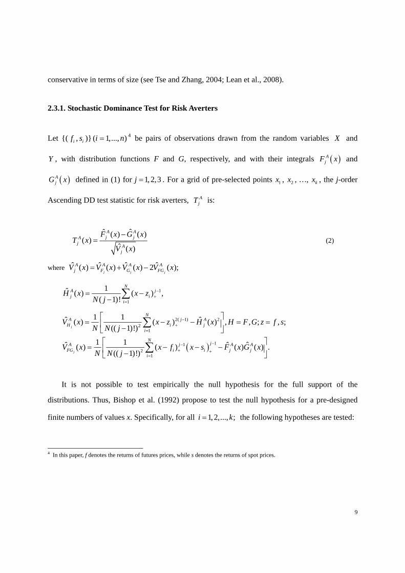
Let {( if , is )} ( 1,..., )i n 4 be pairs of observations drawn from the random variables X and

Y , with distribution functions F and G, respectively, and with their integrals AjF x and

AjG x defined in (1) for 1,2,3j . For a grid of pre-selected points 1x , 2x , …, kx , the j-order

Ascending DD test statistic for risk averters, AjT is:

ˆˆ ( ) ( )( )

ˆ ( )

A Aj jA

jA

j

F x G xT x

V x

(2)

where ˆ ˆ ˆ ˆ( ) ( ) ( ) 2 ( );j j j

A A A Aj F G FGV x V x V x V x

1

1

1ˆ ( ) ( ) ,( 1)!

NA jj i

i

H x x zN j

2( 1) 22

1

112

1

1 1ˆ ˆ( ) ( ) ( ) , , ; , ;(( 1)!)

1 1 ˆˆ ˆ( ) ( ) ( ) ( ) .(( 1)!)

j

j

NA j A

H i ji

NjA j A A

FG i i j ji

V x x z H x H F G z f sN N j

V x x f x s F x G xN N j

It is not possible to test empirically the null hypothesis for the full support of the

distributions. Thus, Bishop et al. (1992) propose to test the null hypothesis for a pre-designed

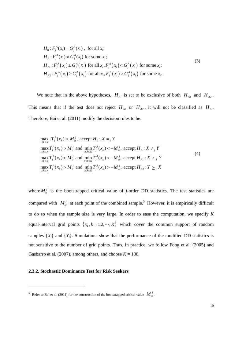
finite numbers of values x. Specifically, for all 1, 2,..., ;i k the following hypotheses are tested:

4 In this paper, f denotes the returns of futures prices, while s denotes the returns of spot prices.

10

0

1

2

: ( ) ( ) , for all ;

: ( ) ( ) for some ;

: for all , for some ;

: for all , for some .

A Aj i j i i

A AA j i j i i

A A A AA j i j i i j i j i i

A A A AA j i j i i j i j i i

H F x G x x

H F x G x x

H F x G x x F x G x x

H F x G x x F x G x x

(3)

We note that in the above hypotheses, AH is set to be exclusive of both 1AH and 2AH .

This means that if the test does not reject 1AH or 2AH , it will not be classified as AH .

Therefore, Bai et al. (2011) modify the decision rules to be:

01

11

111

11

max | ( ) | , accept :

max ( ) and min ( ) , accept :

max ( ) and min ( ) , accept :

max ( ) and min ( )

A jj k j

k K

A j A jj k j k A j

k Kk K

A j A jjj k j k A

k Kk K

A j Aj k j k

k Kk K

T x M H X Y

T x M T x M H X Y

T x M T x M H X Y

T x M T x

2, accept : jjAM H Y X

(4)

where jM is the bootstrapped critical value of j-order DD statistics. The test statistics are

compared with jM at each point of the combined sample.5 However, it is empirically difficult

to do so when the sample size is very large. In order to ease the computation, we specify K

equal-interval grid points Kkxk ,,2,1, which cover the common support of random

samples {Xi} and {Yi}. Simulations show that the performance of the modified DD statistics is

not sensitive to the number of grid points. Thus, in practice, we follow Fong et al. (2005) and

Gasbarro et al. (2007), among others, and choose K = 100.

2.3.2. Stochastic Dominance Test for Risk Seekers

5 Refer to Bai et al. (2011) for the construction of the bootstrapped critical value jM .

11

In order to test SD for risk seekers, the DD statistics for risk averters are modified to be the

Descending DD test statistic, DjT , such that:

ˆˆ ( ) ( )( )

ˆ ( )

D Dj jD

jDj

F x G xT x

V x

(5)

where ˆ ˆ ˆ ˆ( ) ( ) ( ) 2 ( );j j j

D D D Dj F G FGV x V x V x V x

1

1

1ˆ ( ) ( ) ,( 1)!

ND jj i

i

H x z xN j

2( 1) 22

1

112

1

1 1ˆ ˆ( ) ( ) ( ) , , ; , ;(( 1)!)

1 1 ˆˆ ˆ( ) ( ) ( ) ( ) ;(( 1)!)

j

j

ND j D

H i ji

NjD j D D

FG i i j ji

V x z x H x H F G z f sN N j

V x f x s x F x G xN N j

where the integrals DjF x and D

jG x are defined in (1) for 1,2,3j . For 1, 2,..., ,i k the

following hypotheses are tested for risk seekers:

0

1

2

: ( ) ( ) , for all ;

: ( ) ( ) for some ;

: for all , for some ;

: for all , for some .

D Dj i j i i

D DD j i j i i

D D D DD j i j i i j i j i i

D D D DD j i j i i j i j i i

H F x G x x

H F x G x x

H F x G x x F x G x x

H F x G x x F x G x x

and the critical rule for risk seekers can be obtained as in Bai et al. (2011).

Similarly to the situation in testing the Ascending SD test, we follow Fong et al. (2005,

2008) and Lean et al. (2007) to make 10 major partitions with 10 minor partitions within any two

consecutive major partitions in each comparison, and use the simulated critical values in Bai et

12

al. (2011).6 This allows the consistency of both the magnitude and sign of the DD statistics

between any two consecutive major partitions to be examined.

Not rejecting either 0H or AH or DH implies the non-existence of any SD relationship

between X and Y, non-existence of any arbitrage opportunity between these two markets, and that

neither of these markets is preferred to the other. If 1AH ( 2AH ) of order one is accepted, X (Y)

stochastically dominates Y (X) at first order, while if 1DH ( 2DH ) of order one is accepted, asset

X (Y) stochastically dominates Y (X) at first order. In this situation, and under certain regularity

conditions,7 an arbitrage opportunity exists and any non-satiated investors will be better off if

they switch from the dominated to the dominant asset. On the other hand, if 1AH ( 2AH ) [ 1DH

( 2DH )] is accepted at order two (three), a particular market stochastically dominates the other at

second- (third-) order. In this situation, arbitrage opportunity does not exist, and switching from

one asset to another will only increase the risk averters’ [seekers’] expected utility, though not

their expected wealth (Jarrow, 1986; Falk and Levy, 1989; Wong et al. 2008). These results could

be used to infer that market efficiency and market rationality could still hold in these markets

(see Chan et al. (2012) and the references contained therein for further information).

In the above analysis, in order to minimize the Type II error and to accommodate the effect

of almost SD (Leshno and Levy, 2002; Guo et al., 2013), we follow Gasbarro et al. (2007) and

use a conservative 5% cut-off point in checking the proportion of test statistics for statistical

inference. Using a 5% cut-off point, we conclude that one prospect dominates another prospect

only if we find that at least 5% of the statistics are significant.

3. Empirical Results and Discussion

6 Refer to Bai et al. (2011) for further details. 7 Refer to Jarrow (1986) for the conditions.

13

3.1. Mean Variance Analysis

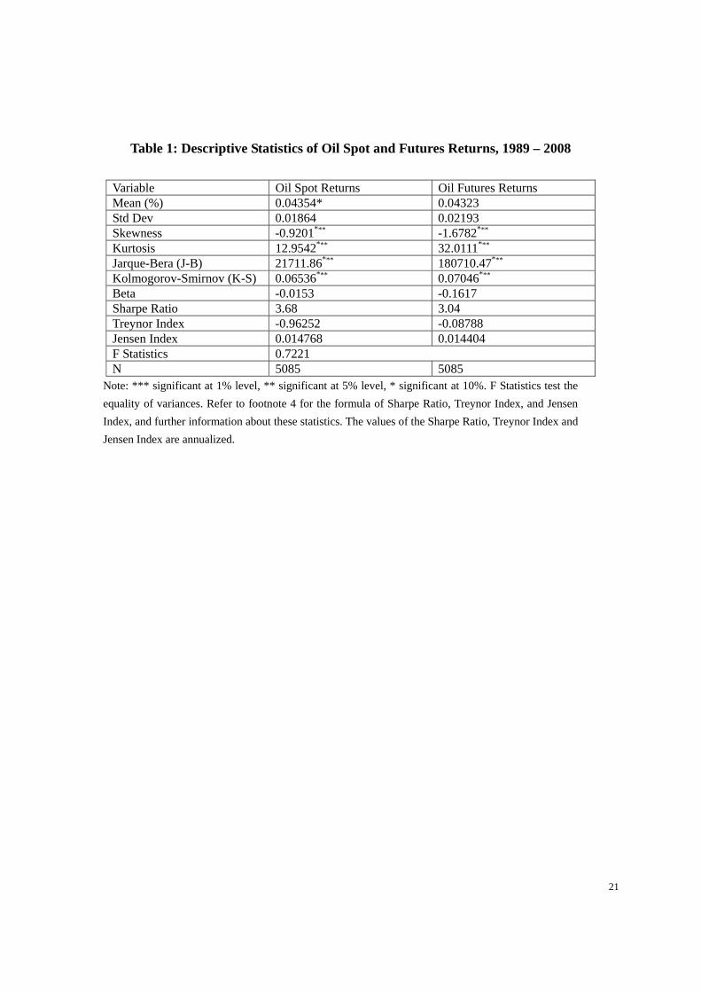
Table 1 provides the descriptive statistics for the daily returns of oil spot prices and oil futures

prices for the entire sample period. The means of their daily returns are about 0.04%, significant

at 10% for the oil spot but not significant for oil futures. From the unreported paired t-tests, the

mean return of oil spot is not significantly higher than that of futures whereas, as expected, its

standard deviation is not significantly smaller than that of futures. As both the means and

standard deviations are not significantly different for the two returns, the MV criterion is unable

to indicate any preference between these two assets.

[Table 1 here]

For the CAPM measures, the absolute value of beta of oil spot returns is smaller than that of

futures, both being negative and less than one. Both returns have similar Sharpe ratios, Treynor

and Jensen indices, with no significant differences between the returns for each statistic. Thus,

the information drawn from the CAPM statistics do not lead to any preference between spot and

futures prices. In addition, the highly significant Kolmogorov-Smirnov (K-S) and Jarque-Bera

(J-B) statistics in Table 1 indicate that both returns are non-normal.8 Moreover, both daily

returns are negatively skewed. As expected, oil futures have much higher kurtosis than spot

prices, with both being higher than under normality. Both skewness and kurtosis indicate

non-normality in the returns distributions, and lead to the conclusion that the normality condition

for the traditional MV and CAPM measures is violated.

3.2. SD Analysis for Risk Averters

8 The results of other normality tests, such as Shapiro-Wilk, lead to the same conclusion. The results are available on request.

14

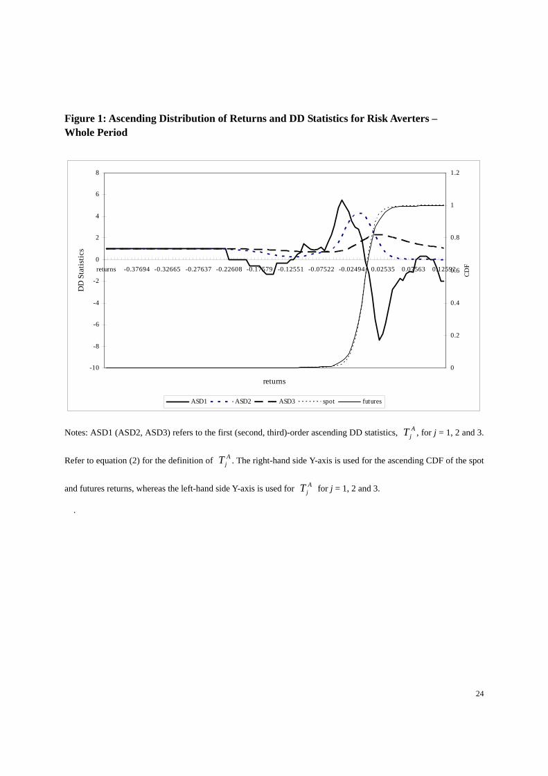
We consider the CDFs of the returns for both oil spot and futures prices and their corresponding

first three orders of the Ascending DD statistics, AjT , for risk averters in Figure 1. If oil futures

dominate spot in the sense of FASD, then the CDF of futures returns should lie significantly

below that of spot prices over the entire range. However, Figure 1 shows that the CDF of spot

lies below that of futures in downside risk, while the CDF of futures lies below that of spot on

upside profit. This indicates that there is no FASD between the two returns, and that spot

dominates futures on downside risk while futures dominate spot on upside profit.

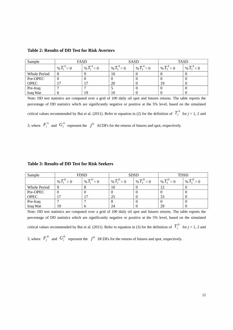
In order to verify this finding formally, we use the first three orders of the Ascending DD

statistics, AjT ( 1, 2,3j ), for the two series, with the results reported in Table 2. DD shows that

the null hypothesis can be rejected if any of the test statistics AjT is significant, and of the

wrong sign.

[Figure 1 here]

The values of 1AT in Figure 1 move from positive to negative along the distribution of

returns. The percentage of significant values reported in Table 2 show that 8% of 1AT is

significantly positive, whereas 9% of 1AT is significantly negative. Thus, the hypotheses that

futures stochastically dominate spot, or vice-versa, at first order are rejected, implying no

arbitrage opportunity between these two series. We can, however, state that oil spot prices

dominate futures in downside returns, while oil futures dominate spot in upside profit.

[Table 2 here]

The SD criterion enables a comparison of utility interpretations in terms of investors’ risk

15

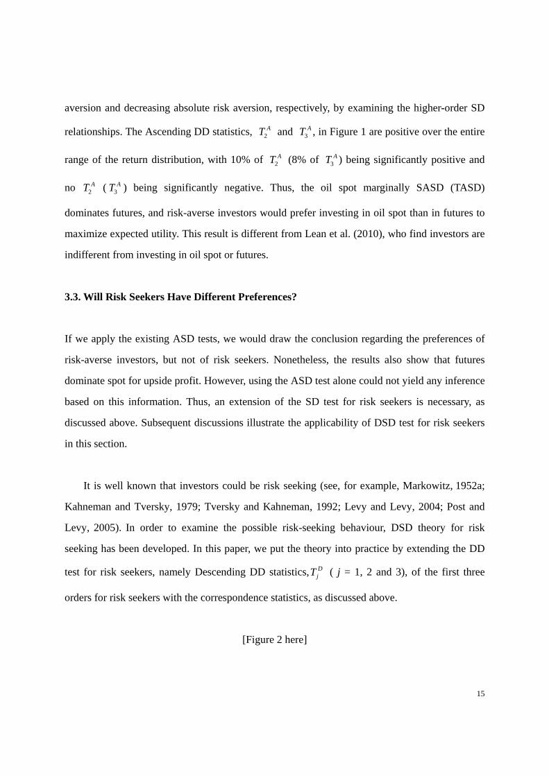
aversion and decreasing absolute risk aversion, respectively, by examining the higher-order SD

relationships. The Ascending DD statistics, 2AT and 3

AT , in Figure 1 are positive over the entire

range of the return distribution, with 10% of 2AT (8% of 3

AT ) being significantly positive and

no 2AT ( 3

AT ) being significantly negative. Thus, the oil spot marginally SASD (TASD)

dominates futures, and risk-averse investors would prefer investing in oil spot than in futures to

maximize expected utility. This result is different from Lean et al. (2010), who find investors are

indifferent from investing in oil spot or futures.

3.3. Will Risk Seekers Have Different Preferences?

If we apply the existing ASD tests, we would draw the conclusion regarding the preferences of

risk-averse investors, but not of risk seekers. Nonetheless, the results also show that futures

dominate spot for upside profit. However, using the ASD test alone could not yield any inference

based on this information. Thus, an extension of the SD test for risk seekers is necessary, as

discussed above. Subsequent discussions illustrate the applicability of DSD test for risk seekers

in this section.

It is well known that investors could be risk seeking (see, for example, Markowitz, 1952a;

Kahneman and Tversky, 1979; Tversky and Kahneman, 1992; Levy and Levy, 2004; Post and

Levy, 2005). In order to examine the possible risk-seeking behaviour, DSD theory for risk

seeking has been developed. In this paper, we put the theory into practice by extending the DD

test for risk seekers, namely Descending DD statistics, DjT ( j = 1, 2 and 3), of the first three

orders for risk seekers with the correspondence statistics, as discussed above.

[Figure 2 here]

16

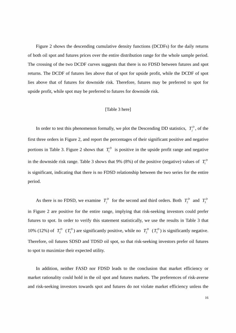
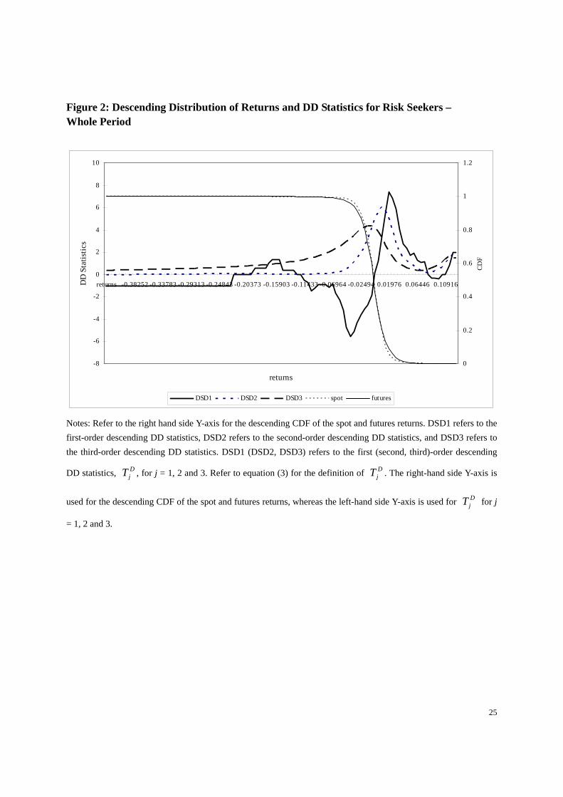
Figure 2 shows the descending cumulative density functions (DCDFs) for the daily returns

of both oil spot and futures prices over the entire distribution range for the whole sample period.

The crossing of the two DCDF curves suggests that there is no FDSD between futures and spot

returns. The DCDF of futures lies above that of spot for upside profit, while the DCDF of spot

lies above that of futures for downside risk. Therefore, futures may be preferred to spot for

upside profit, while spot may be preferred to futures for downside risk.

[Table 3 here]

In order to test this phenomenon formally, we plot the Descending DD statistics, DjT , of the

first three orders in Figure 2, and report the percentages of their significant positive and negative

portions in Table 3. Figure 2 shows that 1DT is positive in the upside profit range and negative

in the downside risk range. Table 3 shows that 9% (8%) of the positive (negative) values of 1DT

is significant, indicating that there is no FDSD relationship between the two series for the entire

period.

As there is no FDSD, we examine DjT for the second and third orders. Both 2

DT and 3DT

in Figure 2 are positive for the entire range, implying that risk-seeking investors could prefer

futures to spot. In order to verify this statement statistically, we use the results in Table 3 that

10% (12%) of 2DT ( 3

DT ) are significantly positive, while no 2DT ( 3

DT ) is significantly negative.

Therefore, oil futures SDSD and TDSD oil spot, so that risk-seeking investors prefer oil futures

to spot to maximize their expected utility.

In addition, neither FASD nor FDSD leads to the conclusion that market efficiency or

market rationality could hold in the oil spot and futures markets. The preferences of risk-averse

and risk-seeking investors towards spot and futures do not violate market efficiency unless the

17

oil market has only one type of investor. These results are consistent with many previous studies

in the literature (see, for example, Fong et al. (2005), who examine the momentum profits in

stocks markets).

From the unreported paired t-tests, the mean return of oil spot is not significantly higher than

that of futures whereas, as expected, its standard deviation is not significantly smaller than that

of futures. As both the means and standard deviations are not significantly different for the two

returns, the MV criterion is unable to indicate any preference between these two assets for risk

seekers.

3.4. The Impact of Oil Crises

Tables 4A and 4B provide the descriptive statistics of the daily returns of oil spot and futures

prices for the OPEC and Iraq War sub-periods. As most of the results of the MV criterion and

CAPM statistics for all sub-periods are similar to those for the full sample period, we discuss

only the results that are different from the full sample period. However, compared with the

pre-OPEC sub-period, the means for both spot and futures returns in the OPEC sub-period

dramatically increased five-fold. On the other hand, compared with the pre-Iraq-War sub-period,

both spot and futures returns in the Iraq-War sub-period were reduced by 90%. Nonetheless, the

differences between the means of spot and futures in each sub-period is still not significant. In

addition, the standard deviations for the returns of spot and futures are also not significantly

different in each of the sub-periods. Thus, similar to the inference to the entire sample, both the

MV criterion and the CAPM statistics are unable to indicate any dominance between the spot and

futures markets.

[Table 4 here]

18

From the DD test, we find that all the values of A

jT and DjT (j = 1, 2 and 3) for both risk

averters and risk seekers are not significant at the 5% level for the first three orders in the

pre-OPEC sub-period. Therefore, there is no arbitrage opportunity in these markets, and both risk

averters and risk seekers are indifferent between these two indices in the pre-OPEC sub-period.

However, in the OPEC sub-period, Table 2 shows that 20% (19%) of 2AT ( 3

AT ) are significantly

positive, and none of the 2AT ( 3

AT ) is significantly negative. Table 3 reveals that 25% (33%) of

2DT ( 3

DT ) are significantly positive, and none of the 2DT ( 3

DT ) is significantly negative at the

5% level. Similar inferences can be drawn for the Iraq War sub-period. Hence, we conclude that,

compared with the full sample period, risk-averse investors prefer the spot index and risk seekers

are attracted to the futures index to maximize their expected utility, though not their expected

wealth, in both the OPEC and Iraq War sub-periods.

3.5. Arbitrage Opportunity, Market Rationality, and Market Efficiency

Without identifying any risk index or any specific model, the SD rules can be used to

determine whether there is any opportunity for arbitrage, and whether markets are efficient and

investors are rational. It is well known (Jarrow, 1986; Falk and Levy, 1989) that, under certain

conditions, if either FASD or FDSD exists, arbitrage opportunities exist, and investors will

increase their wealth and expected utility if they shift from holding the dominated to the

dominant asset. However, Wong et al. (2008) have shown that, if FASD or FDSD exists

statistically, arbitrage opportunities may not exist, but investors can increase their expected

wealth as well as their expected utility if they shift from holding the dominated to the dominant

asset. It is well known from the market efficiency hypothesis that if one is able to earn abnormal

returns, the market is considered to be inefficient. Market efficiency can be tested using SD rules

as follows: if investors can switch their asset choice and increase their expected wealth,

independently of their specific preferences, then market inefficiency is implied.

19

In our analysis, we find that oil spot FSD dominates futures in downside returns, while

futures FSD dominate spot prices in upside returns, spot does not FSD dominate futures over the

entire distribution, and vice-versa, for the entire periods, as well as in all sub-periods. As our

analysis concludes that investors will not increase their expected wealth by switching their

investment from oil futures to spot, or vice-versa, there is no arbitrage opportunity in the oil spot

and futures markets. This implies that there is no arbitrage opportunity in the oil spot and futures

markets for the entire period, as well as in all sub-periods.

Falk and Levy (1989) have shown that, given two assets, X and Y, if by switching from X

to Y (or by selling X short and holding Y long), an investor can increase expected utility, the

market is inefficient. SASD from one prospect, say spot, over another prospect, say futures, does

not imply any arbitrage opportunity, but it does imply the preference of spot over futures by

risk-averse investors. Nonetheless, risk averters would not make an expected profit by switching

from futures to spot, but switching would allow investors to increase their expected utility. A

similar argument can be made for the TASD criterion. This is exactly what is found in the oil

spot and futures markets. Should we claim that the oil spot and futures markets are inefficient

and investors are irrational?

Such a claim could be made if markets have only risk-averse investors. However, it is

well known that markets could have other types of investors (see, for example, Friedman and

Savage, 1948; Markowitz, 1952b; Broll et al., 2010; Egozcue et al., 2011 for further discussion).

Under the assumption that markets could contain more than one type of investor, such as risk

averters and risk seekers, it is possible that one asset dominates another asset by ASD but is

dominated by DSD. These are precisely the findings obtained in this paper. Oil spot stochastically

dominates oil futures strictly in the sense of SASD and TASD, while futures stochastically

dominate spot strictly in the sense of SDSD and TDSD.

20

Therefore, risk averters could prefer to invest in the spot market rather than in futures,

while risk seekers could prefer to invest in futures rather than in the spot market. In equilibrium,

the number of trades that risk averters, who go long in spot and/or short sell futures, would match

the number of trades that risk seekers, who go long in futures and/or short sell spot. In this

situation, there is no upward or downward pressure on prices in the spot or futures market, while

both risk averters and risk seekers could obtain what they want. Under these conditions, we agree

with the assessment in Qiao et al. (2013) that the market remains efficient and that investors are

rational.

4. Conclusion

This paper offered a robust decision tool for investment decisions with uncertainty in oil markets.

The SD tests revealed the existence of arbitrage opportunities, identified the preferences for both

risk averters and risk seekers over different investment prospects, and enabled inferences

regarding market rationality and market efficiency. We applied the DD tests to examine the

behaviour of both risk averters and risk seekers with regard to the Brent crude oil spot and

futures markets, and compared the performances in the two markets.

The empirical results showed conclusively that oil spot dominates oil futures on downside

risk, whereas futures dominate spot on upside profit. We concluded that there is no arbitrage

opportunity and the markets are efficient. In addition, it was shown that oil spot dominates

futures in downside returns, while oil futures dominate spot in upside profit. In addition, we

provided evidence that risk-averse investors prefer oil spot, while risk seekers are attracted to oil

futures in order to maximize their expected utility, though not their expected wealth, for the

entire period, as well as for both the OPEC and Iraq War sub-periods.

21

Table 1: Descriptive Statistics of Oil Spot and Futures Returns, 1989 – 2008

Variable Oil Spot Returns Oil Futures Returns Mean (%) 0.04354* 0.04323 Std Dev 0.01864 0.02193 Skewness -0.9201*** -1.6782***

Kurtosis 12.9542*** 32.0111***

Jarque-Bera (J-B) 21711.86*** 180710.47***

Kolmogorov-Smirnov (K-S) 0.06536*** 0.07046***

Beta -0.0153 -0.1617 Sharpe Ratio 3.68 3.04 Treynor Index -0.96252 -0.08788 Jensen Index 0.014768 0.014404 F Statistics 0.7221 N 5085 5085

Note: *** significant at 1% level, ** significant at 5% level, * significant at 10%. F Statistics test the

equality of variances. Refer to footnote 4 for the formula of Sharpe Ratio, Treynor Index, and Jensen

Index, and further information about these statistics. The values of the Sharpe Ratio, Treynor Index and

Jensen Index are annualized.

22

Table 2: Results of DD Test for Risk Averters Sample FASD SASD TASD

% 1AT > 0 % 1

AT < 0 % 2AT > 0 % 2

AT < 0 % 3AT > 0 % 3

AT < 0

Whole Period 8 9 10 0 8 0 Pre-OPEC 0 0 0 0 0 0 OPEC 17 17 20 0 19 0 Pre-Iraq 7 7 5 0 0 0 Iraq War 6 19 10 0 0 0 Note: DD test statistics are computed over a grid of 100 daily oil spot and futures returns. The table reports the

percentage of DD statistics which are significantly negative or positive at the 5% level, based on the simulated

critical values recommended by Bai et al. (2011). Refer to equation in (2) for the definition of A

jT for j = 1, 2 and

3, where A

jF and AjG represent the thj ACDFs for the returns of futures and spot, respectively.

Table 3: Results of DD Test for Risk Seekers Sample FDSD SDSD TDSD

% 1DT > 0 % 1

DT < 0 % 2DT > 0 % 2

DT < 0 % 3DT > 0 % 3

DT < 0

Whole Period 9 8 10 0 12 0 Pre-OPEC 0 0 0 0 0 0 OPEC 17 17 25 0 33 0 Pre-Iraq 7 7 8 0 0 0 Iraq War 19 6 24 0 29 0 Note: DD test statistics are computed over a grid of 100 daily oil spot and futures returns. The table reports the

percentage of DD statistics which are significantly negative or positive at the 5% level, based on the simulated

critical values recommended by Bai et al. (2011). Refer to equation in (3) for the definition of DjT for j = 1, 2 and

3, where DjF and

DjG represent the thj DCDFs for the returns of futures and spot, respectively.

23

Table 4A: Descriptive Statistics of Oil Spot Prices and Oil Futures Prices for Sub-Periods Pre-OPEC OPEC Variable Oil Spot Prices Oil Futures Prices Oil Spot Prices Oil Futures Prices Mean (%) 0.01287 0.01185 0.08185** 0.08242* Std Dev 0.01969 0.02240 0.01723 0.02134 Skewness -1.08807*** -2.6108*** -0.5726 -0.3245 Kurtosis 17.4315*** 51.5032*** 2.5760 2.1657 J-B 25063.69* 280027.11*** 140.526 105.264 K-S 0.08918* 0.1069*** 0.05249*** 0.03683***

Beta 0.01124 -0.3738 -0.03372 -0.00047 Sharpe Ratio -0.8875 -1.0375 10.35 8.45 Treynor Index -0.33592 0.01326 -1.1232 -81.9728 Jensen Index -4108 -0.00203 0.037648 0.038168 F Statistics 0.7726 0.6523 N 2824 2824 2261 2261 Note: *** significant at 1% level, ** significant at 5% level, * significant at 10%. F Statistics test the equality of

variances. Refer to footnote 4 for the formula of the Sharpe Ratio, Treynor Index, and Jensen Index, and further

information about these statistics. The values of the Sharpe Ratio, Treynor Index and Jensen Index are annualized.

Table 4B: Descriptive Statistics of Oil Spot Prices and Oil Futures Prices for Sub-Periods Pre-Iraq War Iraq War Variable Oil Spot Prices Oil Futures Prices Oil Spot Prices Oil Futures Prices Mean (%) 0.01566 0.01339 0.001184*** 0.001200** Std Dev 0.01956 0.02284 0.01586 0.01932 Skewness -1.01998*** -2.03499*** -0.2882*** 0.02237 Kurtosis 14.2659*** 37.07080*** 1.4916*** 0.7288*** J-B 20252.50*** 181905.92*** 149.716*** 296.282*** K-S 0.07501*** 0.09179*** 0.04717*** 0.02983*** Beta 0.02377 0.1861 -0.1645 -0.07809 Sharpe Ratio 0.3443 -0.65 17.24 14.35 Treynor Index 0.001172 0.0003267 -0.006794 -0.01452 Jensen Index -2.66*10-5 -7.09*10-5 0.001155 0.001152 F Statistics 0.7338 0.67425 N 3708 3708 1378 1378 Note: *** significant at 1% level, ** significant at 5% level, * significant at 10%. F Statistics test the equality of

variances. Refer to footnote 4 for the formula of the Sharpe Ratio, Treynor Index, and Jensen Index, and further

information about these statistics. The values of the Sharpe Ratio, Treynor Index and Jensen Index are annualized.

24

Figure 1: Ascending Distribution of Returns and DD Statistics for Risk Averters – Whole Period

-10

-8

-6

-4

-2

0

2

4

6

8

returns -0.37694 -0.32665 -0.27637 -0.22608 -0.17579 -0.12551 -0.07522 -0.02494 0.02535 0.07563 0.12592

returns

DD

Sta

tist

ics

0

0.2

0.4

0.6

0.8

1

1.2

CD

F

ASD1 ASD2 ASD3 spot futures

Notes: ASD1 (ASD2, ASD3) refers to the first (second, third)-order ascending DD statistics, AjT , for j = 1, 2 and 3.

Refer to equation (2) for the definition of AjT . The right-hand side Y-axis is used for the ascending CDF of the spot

and futures returns, whereas the left-hand side Y-axis is used for AjT for j = 1, 2 and 3.

.

25

Figure 2: Descending Distribution of Returns and DD Statistics for Risk Seekers – Whole Period

-8

-6

-4

-2

0

2

4

6

8

10

returns -0.38252 -0.33783 -0.29313 -0.24843 -0.20373 -0.15903 -0.11433 -0.06964 -0.02494 0.01976 0.06446 0.10916

returns

DD

Sta

tist

ics

0

0.2

0.4

0.6

0.8

1

1.2

CD

F

DSD1 DSD2 DSD3 spot futures

Notes: Refer to the right hand side Y-axis for the descending CDF of the spot and futures returns. DSD1 refers to the

first-order descending DD statistics, DSD2 refers to the second-order descending DD statistics, and DSD3 refers to

the third-order descending DD statistics. DSD1 (DSD2, DSD3) refers to the first (second, third)-order descending

DD statistics, DjT , for j = 1, 2 and 3. Refer to equation (3) for the definition of D

jT . The right-hand side Y-axis is

used for the descending CDF of the spot and futures returns, whereas the left-hand side Y-axis is used for DjT for j

= 1, 2 and 3.

26

References Anderson, G. (1996). Nonparametric tests of stochastic dominance in income distributions. Econometrica,64, 1183-1193. Arouri, M.E.H., Lahiani, A., Levy, A., Nguyen, D.K. (2012). Forecasting the conditional volatility of oil spot and futures prices with structural breaks and long memory models. Energy Economics, 34, 283-293. Bai, Z. D., Hui, Y.C. Wong, W.K. and Zitikis, R. (2012). Evaluating Prospect Performance: making a Case for a Non-asymptotic UMPU test. Journal of Financial Econometrics, 10(4), 703-732. Bai, Z., Li, H., Liu, H., Wong, W.K. (2011). Test Statistics for Prospect and Markowitz Stochastic Dominances with Applications. Econometrics Journal, 14(2), 278-303 Barrett, G., Donald, S. (2003). Consistent tests for stochastic dominance. Econometrica, 71, 71-104. Beedles, W.L. (1979). Return, dispersion and skewness: synthesis and investment strategy. Journal of Financial Research, 2, 71-80. Bekiros, S.D., Diks, C.G.H. (2008). The Relationship between Crude Oil Spot and Futures Prices: Cointegration, Linear and Nonlinear Causality. Energy Economics, 30(5), 2673-2685. Bishop, J.A., Formly, J.P., Thistle, P.D. (1992). Convergence of the South and non-South income distributions. American Economic Review, 82, 262-272. Bopp, A.E., Sitzer, S. (1987). Are petroleum futures prices good predictors of cash value? Journal of Futures Markets, 7, 705-719. Broll, U., Egozcue, M., Wong, W.K., and Zitikis, R. (2010). Prospect theory, indifference curves, and hedging risks. Applied Mathematics Research Express, 2, 142-153. Chan, C.Y., Christian de Peretti, C., Qiao, Z., Wong, W.K. (2012). Empirical Test of the Efficiency of UK Covered Warrants Market: Stochastic Dominance and Likelihood Ratio Test Approach. Journal of Empirical Finance, 19(1), 162-174. Crowder, W.J., Hamid, A. (1993). A co-integration test for oil futures market efficiency. Journal of Futures Markets, 13, 933-941.

27

Cumby, R.E., Glen, J.D. (1990). Evaluating the performance of international mutual funds. Journal of Finance, 45(2), 497-521. Davidson, R., Duclos, J-Y. (2000). Statistical inference for stochastic dominance and for the measurement of poverty and inequality. Econometrica, 68, 1435-1464. Egozcue, M., Fuentes García, L., Wong, W.K., and Zitikis, R. (2011), Do investors like to diversify? A study of Markowitz preferences, European Journal of Operational Research, 215(1), 188-193. Falk, H., Levy, H. (1989). Market reaction to quarterly earnings' announcements: A stochastic dominance based test of market efficiency. Management Science, 35, 425-446. Fishburn, P.C. (1964). Decision and Value Theory, New York. Fong, W.M., Lean, H.H., Wong, W.K. (2008). Stochastic dominance and behavior towards risk: the market for internet stocks. Journal of Economic Behavior and Organization, 68(1), 194-208. Fong, W.M., See, K.H. (2003). Basis variations and regime shifts in the oil futures market. The European Journal of Finance, 9, 499-513. Fong, W.M., Wong, W.K., Lean, H.H. (2005). International momentum strategies: A stochastic dominance approach. Journal of Financial Markets, 8, 89-109. Friedman, M., Savage, L.J. (1948), The Utility Analysis of Choices Involving Risk. Journal of Political Economy, 56, 279-304. Gasbarro, D., Wong, W.K., Zumwalt, J.K. (2007). Stochastic dominance analysis of iShares. European Journal of Finance, 13, 89-101. Guo, X., Zhu, X.H., Wong, W.K., Zhu, L.X. (2013). A Note on Almost Stochastic Dominance. Economics Letters, forthcoming. Gulen, S.G., (1999). Regionalization in world crude oil markets: further evidence. Energy Journal, 20, 125-139. Hadar J., Russell, W.R. (1969). Rules for ordering uncertain prospects. American Economic Review, 59, 25-34. Hammond, J.S., (1974). Simplifying the choice between uncertain prospects where preference is nonlinear. Management Science, 20(7), 1047-1072.

28

Hammoudeh, S., Li, H., Jeon, B. (2003). Causality and volatility spillovers among petroleum prices of WTI, gasoline and heating oil in different locations. North American Journal of Economics and Finance, 14, 89-114. Hanoch, G., Levy, H. (1969). The efficiency analysis of choices involving risk. Review of Economic studies, 36, 335-346. Jarrow, R. (1986). The relationship between arbitrage and first order stochastic dominance. Journal of Finance, 41, 915-921. Jensen, M.C. (1969). Risk, the pricing of capital assets and the evaluation of investment portfolios. Journal of Business, 42, 167-247. Kahneman, D., Tversky, A. (1979). Prospect theory of decisions under risk. Econometrica, 47(2), 263-291. Kang, S.H., Kang, S.M. and Yoon, S.M. (2009). Forecasting volatility of crude oil markets. Energy Economics, 31, 119-125. Kaur, A., Rao, B.L.S.P., Singh, H. (1994). Testing for second order stochastic dominance of two distributions. Econometric Theory, 10, 849-866. Klecan, L., McFadden, R., McFadden, D. (1991). A robust test for stochastic dominance. Working Paper, MIT & Cornerstone Research. Lean, H.H., McAleer, M., Wong, W.K. (2010). Market efficiency of oil spot and futures: A mean-variance and stochastic dominance approach. Energy Economics, 32, 979-986. Lean, H.H., Smyth, R., Wong, W.K. (2007). Revisiting calendar anomalies in Asian stock markets using a stochastic dominance approach. Journal of Multinational Financial Management, 17(2), 125-141. Lean, H.H., Wong, W.K., Zhang, X. (2008). Size and Power of Some Stochastic Dominance Tests: A Monte Carlo Study. Mathematics and Computers in Simulation, 79, 30-48. Leshno, M. and H. Levy. (2002). Preferred by “All” and preferred by “Most” decision makers: Almost stochastic dominance. Management Science, 48, 1074-1085. Leung, P.L., Wong, W.K. (2008). On Testing the Equality of the Multiple Sharpe Ratios, with Application on the Evaluation of IShares. Journal of Risk, 10(3), 1-16.

29

Levy, H., Levy, M. (2004). Prospect theory and mean-variance analysis. Review of Financial Studies, 17(4), 1015-1041. Li, C.K., Wong, W.K. (1999). A note on stochastic dominance for risk averters and risk takers. RAIRO Recherche Operationnelle, 33, 509-524. Lin, X.S., Tamvakis, M.N. (2001). Spillover effects in energy futures markets. Energy Economics, 23, 43-56. Linton, O., Maasoumi, E., Whang, Y-J. (2005). Consistent testing for stochastic dominance under general sampling schemes. Review of Economic Studies, 72, 735-765. Markowitz, H.M. (1952a). Portfolio selection. Journal of Finance, 7, 77-91. Markowitz, H.M. (1952b), The Utility of Wealth. Journal of Political Economy, 60, 151-156. McFadden, D. (1989). Testing for stochastic dominance. In: T.B. Fomby and T.K. Seo, (Eds.), Studies in the Economics of Uncertainty. Springer Verlag, New York. Morey, M.R., Morey, R.C. (2000). An analytical confidence interval for the Treynor index: formula, conditions and properties. Journal of Business Finance & Accounting, 27(1) & (2), 127-154. Post, T., Levy, H. (2005). Does risk seeking drive asset prices? A stochastic dominance analysis of aggregate investor preferences and beliefs. Review of Financial Studies, 18(3), 925-953. Qiao, Z., Clark, E., Wong, W.K. (2013). Investors’ Preference towards Risk: Evidence from the Taiwan Stock and Stock Index Futures Markets. To appear in Accounting & Finance. Quirk J.P., Saposnik, R. (1962). Admissibility and measurable utility functions. Review of Economic Studies, 29, 140-146. Rothschild, M., Stiglitz, J.E. (1970). Increasing risk I. A definition. Journal of Economic Theory, 2, 225-243. Schwartz, T.V., Szakmary, A.C. (1994). Price discovery in petroleum markets: arbitrage, cointegration and the time interval of analysis. Journal of Futures Markets, 14, 147-167. Sharpe, W.F. (1964). Capital asset prices: Theory of market equilibrium under conditions of risk. Journal of Finance 19, 425-442.

30

Sriboonchitta, S., Wong, W.K., Dhompongsa, S., Nguyen, H.T. (2009). Stochastic Dominance and Applications to Finance, Risk and Economics, Chapman and Hall/CRC, Taylor and Francis Group, Boca Raton, Florida, USA. Tesfatsion, L. (1976). Stochastic dominance and maximization of expected utility. Review of Economic Studies, 43, 301-315. Treynor, J.L. (1965). How to rate management of investment funds. Harvard Business Review, 43, 63-75. Tse, Y.K., Zhang, X. (2004). A Monte Carlo investigation of some tests for stochastic dominance. Journal of Statistical Computation and Simulation, 74, 361-378. Tversky, A., Kahneman, D. (1992). Advances in prospect theory: Cumulative representation of uncertainty. Journal of Risk and Uncertainty, 5, 297-323. Wilson, B., Aggarwal, R., Inclan, C. (1996). Detecting volatility changes across the oil sector. Journal of Futures Markets, 16, 313-320.

Wong, W.K. (2007). Stochastic dominance and mean-variance measures of profit and loss for

business planning and investment. European Journal of Operational Research, 182, 829-843.

Wong, W.K., Chan, R.H. (2008). Markowitz and prospect stochastic dominances. Annals of Finance, 4(1), 105-129. Wong, W.K., Li, C.K. (1999). A note on convex stochastic dominance theory. Economics Letters, 62, 293-300. Wong, W.K. Ma, C. (2008). Preferences over location-scale family. Economic Theory, 37(1), 119-146. Wong, W.K., Phoon, K.F., Lean, H.H. (2008). Stochastic dominance analysis of Asian hedge funds. Pacific-Basin Finance Journal, 16(3), 204-223.