Risk Assessment of Oil Spills to US Inland Waterways

Advances in Financial Mathematics 01/2014

Normal Expansion of SABR

Philippe Balland, UBS

[email protected] ppg.balland:gmail.com

Normal Expansion of SABR Advances in Financial Mathematics 01/2014 Philippe Balland - page 2

Introduction

Historical and implied backbones define the ‘expected’ relationship between swap rates and ATM volatilities:

Typical interest rates have a backbone closer to normal than lognormal:

The SABR formula is based on an asymptotic expansion of the Lognormal implied volatility. However, this

formula becomes inaccurate and can imply negative density when the elasticity parameter is small. We

propose to resolve this issue by performing an asymptotic expansion of the Normal SABR implied volatility

instead.


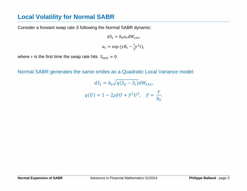
Local Volatility for Normal SABR

Consider a forward swap rate S following the Normal SABR dynamic:

where is the first time the swap rate hits .

Normal SABR generates the same smiles as a Quadratic Local Variance model:


Local Volatility for Normal SABR: Proof

The local volatility is calculated as follows:

Calculation of L:

Define:

Observe:

By Ito’s lemma, derive:


Calculation of D:

Define:

Similarly to above:

Define and derive:

Consider the probability measure such that

:

Obtain the following expression for D:

Derive by grouping the terms for D and L:


Local Volatility for SABR

Consider a forward swap rate S following the SABR dynamic:

SABR and the below Local Volatility model imply similar smiles:

This result is obtained using the same calculation as the one explained above for the Local Volatility for

Normal SABR. Details can also be found in P. Balland and Q. Tran, 'SABR goes normal', Risk, June 2013.


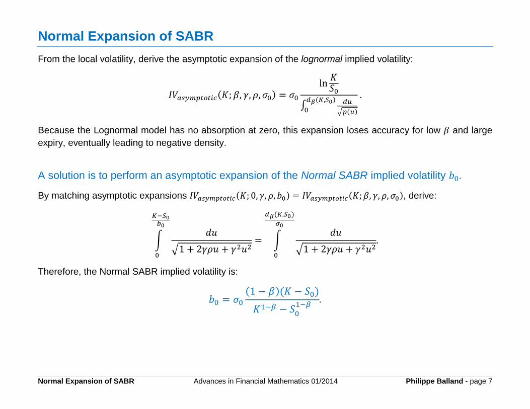
Normal Expansion of SABR

From the local volatility, derive the asymptotic expansion of the lognormal implied volatility:

Because the Lognormal model has no absorption at zero, this expansion loses accuracy for low and large

expiry, eventually leading to negative density.

A solution is to perform an asymptotic expansion of the Normal SABR implied volatility

By matching asymptotic expansions , derive:

Therefore, the Normal SABR implied volatility is:


Pricing Formula for Normal SABR

Replace Normal SABR by the Quadratic Local Variance process:

where is the first time the process hits the boundary .

Apply the Tanaka-Meyer formula:

Define:

Calculate:


Resolve the drift by changing measure to with

.

Derive:

Observe that satisfies

Derive:

Finally, obtain:

,


Numerical Implementation

Choose a grid such that :

The integrals can be analytically calculated at a cost similar to two cumulative normal calculations using the

formula 7.4.33 in M. Abramowitz and I.A. Stegun, Handbook of Mathematical Functions, 1972.

Simplify the calculation of with the following approximation:


Numerical Calculation of

Calculate

on a set of N(0,1)-nodes :

Use and the symmetric Hermite nodes that appear in the Gauss-Hermite integration:

The Hermite nodes associated with are:

Calculate by forward induction:

The conditional expectation can be analytically computed since and

are unit normal variables with

correlation

.

-3.775611 -2.516917 -1.50041 -0.682802 -0.141764 0.141764 0.682802 1.50041 2.516917 3.775611


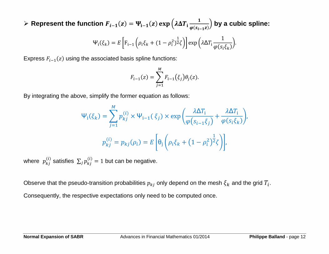
Represent the function

by a cubic spline:

Express using the associated basis spline functions:

By integrating the above, simplify the former equation as follows:

where

satisfies

but can be negative.

Observe that the pseudo-transition probabilities only depend on the mesh and the grid .

Consequently, the respective expectations only need to be computed once.


Analytical Calculation of the Pseudo-Transition Probabilities

The function is a cubic spline with value zero at every node except at where it takes value one:

where are calculated using the standard cubic spline algorithm.

Finally, compute the pseudo-transition probabilities:

where .

By integration:


Numerical Results

With standard market conditions, just a few steps N and states M are needed to obtain accurate call prices.

With we obtain the following results where the implied volatility is displayed as a function of the

lognormal standard deviation defined as

:

-0.4

-0.2

0

0.2

0.4

0.6

0.8

-8 -6 -4 -2 0 2 4 6

SABR density

Normal-SABR implied-vol

Normal-SABR density

NormalSABR with g=40%, r=0.4, b=0.2, ATM=27%, T=20yr

Risk Assessment of Oil Spills to US Inland Waterways

Documents

Transcript of Risk Assessment of Oil Spills to US Inland Waterways