CFR-Working Paper NO. 04-03

Risk and Return in Convertible Arbitrage: Evidence from the

Convertible Bond Market

V. Agarwal • W. H. Fung • Y. C. Loon • N. Y. Naik

Risk and Return in Convertible Arbitrage: Evidence from the Convertible Bond

Market

Vikas Agarwal a, b, 1, William H. Fung c, 2 , Yee Cheng Loon d, 3 , Narayan Y. Naik c,*

Forthcoming in the Journal of Empirical Finance

a Georgia State University, J. Mack Robinson College of Business, Atlanta, GA, U.S.A. b Centre for Financial Research (CFR), University of Cologne, Germany c London Business School, London, U.K. d Binghamton University, School of Management, Binghamton, NY, U.S.A. *Corresponding author. London Business School, Sussex Place, Regent's Park, London NW1 4SA, United Kingdom. Tel.: +44-20-7000-8223; fax: +44-20-7000-8201. E-mail addresses: vagarwal@gsu.edu (V. Agarwal), bfung@london.edu (W.H. Fung), ycloon@binghamton.edu (Y.C. Loon), nnaik@london.edu (N.Y. Naik) 1 Tel.: +1-404-413-7326; fax: +1-404-413-7312. 2 Tel.: +44-20-7000-8227; fax: +44-20-7000-8201. 3 Tel.: +1-607-777-2376; fax: +1-607-777-4422.

Abstract

In this paper, we identify and document the empirical characteristics of the key drivers of

convertible arbitrage as a strategy and how they impact the performance of convertible arbitrage

hedge funds. We show that the returns of a buy-and-hedge strategy involving taking a long

position in convertible bonds (“CBs”) while hedging the equity risk alone explains a substantial

amount of these funds’ return dynamics. In addition, we highlight the importance of non-price

variables such as extreme market-wide events and the supply of CBs on performance. Out-of-

sample tests provide corroborative evidence on our model’s predictions. At a more micro level,

larger funds appear to be less dependent on directional exposure to CBs and more active in

shorting stocks to hedge their exposure than smaller funds. They are also more vulnerable to

supply shocks in the CB market. These findings are consistent with economies of scale that

large funds enjoy in accessing the stock loan market. However, the friction involved in adjusting

the stock of risk capital managed by a large fund can negatively impact performance when the

supply of CBs declines. Taken together, our findings are consistent with convertible arbitrageurs

collectively being rewarded for playing an intermediation role of funding CB issuers whilst

distributing part of the equity risk of CBs to the equity market.

Keywords: Hedge funds, Convertible Bonds, Convertible arbitrage, Supply, Risk Factors

JEL classification: G10, G19, G23

1

1. Introduction

At the turn of the century, capitalization of the global convertible bond (“CB”) market

stood at just under $300 billion while the US equity market was more than 50 times higher at

over $1.5 trillion. Yet during the difficult market conditions between 2000 and 2002 (with

events such as end to the dotcom bubble, September 11, and the accounting scandals at

Worldcom and Enron), the new issues in both these markets were of similar orders of

magnitude—close to $300 billion. Even during the financial crisis of 2007-2008, firms managed

to raise about $118 billion in the US CB market.1 This underscores the importance of the CB

market as a source of capital for corporations during adverse economic conditions. 2

To smooth the placement of such a large-scale issuance of CBs, economic agents willing

to assume the inventory risk are clearly needed. Coincident to these macro events, the last

decade has witnessed a rapid growth of convertible arbitrage (“CA”) hedge funds. In spite of the

rapid growth, assets employed by the convertible arbitrage strategy averaged around 4.51% of

assets across all hedge fund strategies between December 1993 and June 2007 (TASS Asset

Flow Report). On the other hand, Mitchell et al. (2007) point out that convertible arbitrage and

other hedge funds make up about 75% of the convertible market. Accounts in the financial press

support this view; for example, Pulliam (2004) notes that in 2003, CA hedge funds purchased

about 80% of newly issued convertible bonds. Brown et al. (2010) document that a large fraction 1 Equity data are from Federal Reserve Bulletin (various issues). We thank Jeff Wurgler for making it available on his website http://pages.stern.nyu.edu/~jwurgler/. CB estimate is from the public and private proceeds of convertible debt from Thomson Reuters Financial’s SDC Platinum database, which we also use later on for our out-of-sample analysis. 2 Apart from being a useful source of liquidity to issuers during adverse market conditions, the issuance of CBs depends also on the costs and benefits compared to other forms of securities issuance. Firms selling CBs incur costs including issuance costs (e.g., underwriter fees and discounts) and dilution of existing stockholders’ interest upon conversion. Firms can also enjoy certain benefits from issuing CBs. These include reduction in the agency cost of debt (Green, 1984; Jensen and Meckling, 1976), mitigation of underinvestment problem due to adverse selection (Brennan and Kraus, 1987; Brennan and Schwartz, 1988; Constantinides and Grundy, 1989), avoidance of high costs of direct equity sales (Brown et al., 2010; Stein, 1992), and reduction of the costs of sequential financing while controlling overinvestment incentives (Mayers, 1998). Firms will only issue CBs if these benefits exceed the costs of issuing CBs.

2

of convertible issues are sold to hedge funds by issuers with greater stock volatility and higher

probability of financial distress, thereby avoiding high costs of issuing equity, which will be even

greater during poor market condition. Among different hedge fund strategies, while CA may not

be the strategy with the largest assets under management (being naturally limited by the supply

of CBs in the market), CA hedge funds do play a significant role in funding the convertible bond

market.

In this paper, we posit that a typical CA hedge fund manager assumes the role of an

intermediary—financing the CB issuers while distributing part of the equity risk of CB

ownership to the equity market through delta hedging. To test our hypothesis, we explicitly

model a commonly used trading strategy that gives us direct insight into the performance of CA

hedge funds. Specifically, we assume that CA hedge funds take a long position in the CBs and

mitigate the inherent equity risk by shorting the equity of the CB issuers. We demonstrate

empirically that such a model explains a substantial amount of CA hedge funds’ return dynamics.

More specifically, our model has two main components—passive and active. The

passive component is similar to the “buy-and-hold” strategy commonly used by mutual funds,

while the active component resembles the “buy-and-hedge” strategy used by hedge funds. The

passive component differs from the active component in two dimensions--leverage and risk

management. Since mutual funds rarely use leverage (e.g., Almazán et al. (2004)), the amount of

liquidity they provide to CB issuers is limited to the amount of assets they manage. In contrast,

through the use of leverage, CA hedge funds can purchase a quantity of CBs well in excess of

their capital and therefore can provide greater liquidity to the CB issuers. 3 From a risk

3 Anecdotal evidence suggests that some CA hedge funds employ a leverage ratio of up to $5 borrowing to $1 equity (Zuckerman (2008)). Gupta and Liang (2005) apply the Value-at-Risk Approach to evaluate the capital adequacy of hedge funds and find that convertible arbitrage funds are better capitalized than funds in emerging markets, long/short equity, and managed futures categories.

3

management perspective, unlike CB mutual funds that typically do not short securities, CA

hedge funds can hedge the equity risk embedded in the CBs by shorting stocks. Thus, unlike

mutual funds, CA hedge funds can use leverage and provide much more liquidity to CB issuers

at only moderate levels of overall portfolio risk. We capture these two dimensions by specifying

a “buy-and-hedge” strategy, which involves buying CBs at issuance and holding them until

maturity (or till the end of our sample period, whichever is earlier) and shorting the shares of the

CB issuers to hedge the equity risk.4

As a funding intermediary for CB issuers, a convertible arbitrageur’s performance

depends on the supply of CBs as well as discrete liquidity events such as the Long Term Capital

Management (LTCM) crisis. The supply of CBs will affect the investment opportunities and

therefore profitability of CA funds. Liquidity events can negatively impact CA funds’ ability to

borrow short-term capital from brokers and raise long-term capital from investors thereby

adversely affecting their ability to effectively implement the CA strategy. Therefore, liquidity

events can also affect the risk appetite of arbitrageurs. We test these hypotheses by incorporating

the impact of changes in supply conditions and major market events while modeling the return of

CA hedge funds.

Using the daily prices of 1,646 US CBs from January 1993 to April 2003, we have five

major findings. First, we show that a combination of buy-and-hold and buy-and-hedge strategies

explains a significant proportion of the variation in CA hedge fund returns. In addition, we show

empirically that the returns of CA hedge funds are positively related to the supply of CBs.

Second, responding to adverse liquidity events, we show that after the LTCM crisis, CA hedge

funds do reduce their reliance on the buy-and-hold strategy thereby paring their directional

4 Since we cannot directly observe the extent to which CA hedge funds actively hedge the equity risk as opposed to buying and holding CBs, we allow for both the passive and active components in our model and empirically estimate their relative importance in determining the CA funds’ performance.

4

exposure to the CB market. Third, combining both supply conditions and market events, we find

alphas to be either insignificant or negative and significant. At first glance, persistent negative

alphas appear to be at odds with the growth in CA funds. We show empirically that these

observed negative alphas depend on the assumption underlying the monetization of specific

measures of CB supply. Fourth, we find that larger funds rely more on the buy-and-hedge factor

relative to the buy-and-hold factor, and are affected more by supply shocks. This is consistent

with economies of scale that large funds enjoy in accessing the stock loan market. However, the

friction involved in adjusting the stock of risk capital managed by a large fund can negatively

impact performance when the supply of CBs declines. Finally, going beyond the data used to

calibrate our model which ended in April 2003, we are able to corroborate the in-sample results

by using a different out-of-sample data source spanning the period May 2003 to June 2007.

Our paper contributes to the growing literature on identifying risk factors that drive

different hedge fund strategies’ returns such as trend-following strategy (Fung and Hsieh (2001)),

merger arbitrage strategy (Mitchell and Pulvino (2001)), equity-oriented hedge fund strategies

(Agarwal and Naik (2004)), equity pairs trading strategy (Gatev et al. (2006)), and fixed income

arbitrage strategy (Duarte et al. (2007); Fung and Hsieh (2004)). Our empirical findings

complement the recent work of Choi et al. (2009) and Choi et al. (2010). Choi et al. (2009) find

that short selling of equity securities by CA hedge funds improves stock liquidity but does not

affect price efficiency after CB issuance. Choi et al. (2010) analyze how the supply of capital

from CA funds affects CB issuance activity. In this paper, we show in an integrated framework

that CA hedge funds short stocks as part of their risk management process, as distinct from

speculative motives, and that the supply of CB issuance in turn impacts these funds’ performance.

5

The rest of the paper is organized as follows. Section 2 describes the data. Section 3

outlines the models of CA strategies used by CA hedge funds. Section 4 provides a description

of our empirical methodology and our findings during the sample period. Section 5 discusses

results from fund level regressions. Section 6 describes findings from our out-of-sample analysis

and Section 7 concludes the paper.

2. Data

The initial sample of daily CB data comprises 2,243 US dollar-denominated CBs kindly

provided to us by Albourne Partners, London.5 From this data set we are able to recover 1,646

CBs over the sample period from January 1993 to April 2003 that have complete contractual

information and daily closing prices needed for our empirical analysis. Table 1 provides

descriptive statistics of our sample. Panel A shows that there are 1,224 firms issuing a total of

1,646 CBs with a majority of the firms having a single CB issue. Panel B reports statistics on

issue size. The mean and median issue sizes are $323 million and $175 million, respectively.

Panel C tracks the growth in the number of CB issues in our sample. The issuance activity in the

US increased steadily from 91 issues in 1993 to 179 issues in 2002, reaching the peak of 211

issues and 265 issues in 1997 and 2001 respectively.6 This variation in the supply of CBs has

important implications for the investment opportunity of CA hedge funds--an issue we explore in

Section 4.2 of the paper.

5 In an earlier version of our paper, we had conducted the entire analysis using Japanese CB data as well. Our results were similar for Japan but for the sake of brevity, we focus only on the analysis with the US bonds here. It would be interesting to examine the structural differences between different CB markets by including Europe too. These issues are part of our ongoing research agenda. 6 Since our sample period ends in April 2003, the issuance figures for 2003 are not comparable to the other years.

6

3. A model of convertible arbitrage strategies

In order to capture the dynamic nature of hedge fund strategies, Fung and Hsieh (1997)

put forward a model where a portfolio of hedge funds can be represented as a linear combination

of a set of basic, synthetic hedge fund strategies. Ideally, these synthetic hedge fund strategies

are rule-based constructs involving only observable asset prices, and are similar in concept to the

familiar Carhart (1997) and Fama and French (1993) long-short factors used in conventional

asset pricing models. Our model is a variation of this approach adapted for CA hedge funds.

However, our research application is in a market in which transaction costs need to be

incorporated. This departure from previous research methodology is described in the next

section where we specify the structure of our model.

3.1. A buy-and-hedge strategy—the X factor

In the spirit of Fung and Hsieh (2001, 2004), we construct a single asset-based-style

(ABS) factor using all new CB issues to create a hedged CB portfolio over time. This involves

forming an issue-size-weighted portfolio of CBs by buying each CB at the first available price

and holding it till its natural maturity or till the end of the sample, whichever comes first.7 This

simplified model has the benefit of having well-defined entry and exit points for the arbitrageurs

and avoids complex and often costly secondary market trading strategies. Equity risk is estimated

by computing the daily return on an issue-size-weighted portfolio of the underlying stocks

associated with each CB in the portfolio – denoted as EQt.

The idea behind using issue-size-weighting is two-fold. First, in terms of transaction

costs, issue-size-weighting avoids the frequent and prohibitively expensive rebalancing induced

7 By natural maturity, we mean the point at which either the bond was converted to equity or redeemed by the issuer. In either case, there will be an exit price recorded in our data sample as in the case of a maturing bond where the initial principal is returned to the bond holder.

7

by daily bond price changes in an equally- (dollar-) weighted portfolio. Second, issue-size-

weighting gives more weight to larger issues reflecting the impact of CB availability on

arbitrageurs’ returns. Note that our approach differs from a market-value weighted portfolio with

a constant amount of capital invested. By increasing the invested capital of the hedged CB

portfolio as new issues arrive, we avoid the need to sell existing holdings to make room for new

issues that a fixed capital method entails. There is, however, an implicit assumption that CA

hedge fund managers, in aggregate, are able to absorb new CB issues through capital infusion

from their investors, through increased leverage, or both.

The buy-and-hedge strategy involves dynamically hedging the equity risk of the CB

portfolio.8 For this purpose, we estimate the hedge ratios for equity risk by estimating the

following regression over a 30-day rolling window:

, 0 1CB t t tR EQg g u= + + (1)

where ,CB tR is the day t return on the issue-size-weighted portfolio of CBs. The return on the

buy-and-hedge strategy equals that on a long position in newly issued CBs and that on a short

position in the corresponding stocks. The hedge ratios (or the short positions) are given by the

slope estimates in equation (1).

8 Since CBs are also exposed to interest rate and credit risks, CA funds may also hedge these two risks in addition to the equity risk. Chan and Chen (2007), Davis and Lischka (1999), and Das and Sundaram (2004), among others, examine the impact of credit and interest rate risks on convertible bond pricing. We examine this variation of the buy-and-hedge strategy later in the paper. Further, CBs also may be subject to the risk of issuer calling the bonds. See for example Brennan and Schwartz (1977, 1980), Buchan (1997), Davis and Lischka (1999), Das and Sundaram (2004), Ingersoll (1977), McConnell and Schwartz (1986), and Tsiveriotis and Fernandes (1998). Brennan and Schwartz (1977, 1980) and Ingersoll (1977) also consider the optimal call strategies for convertible bonds. It is not obvious that call risk is a significant risk to CA funds. First, CB prices already reflect the likelihood of redemption (e.g., by trading at parity less the accrued interest). Second, there are also behavioral aspects of market agents that are hard to quantify. For example, Woodson (2002, p.28) notes that convertible issuers in Japan usually do not call their bonds to avoid upsetting their investors. Although this practice may be suboptimal with respect to short-term shareholder wealth maximization, it does suggest that CA funds are only subject to a limited amount of call risk in practice.

8

To capture the transaction costs in a buy-and-hedge strategy, we assume that the long

position is financed by borrowing at the discount rate, DISCt, which is proxied by the Fed Funds

rate. The interest due on the cash balance from short positions in the underlying stocks (referred

to as short rebate) is assumed to be at a lower rate than the borrowing rate by a spread, s, (or

haircut) – for simplicity, we assume this to be 50 basis points for the US market.9 Another way of

interpreting this 50 basis point spread is to think of it as the prime broker’s debit/credit spread for

lending against the CB while paying interest on the cash balance from the short sale. This way,

the reference level of interest rate cancels and the net cost to the CA hedge fund is this

debit/credit spread of 50 basis points.10

After adjusting for these financing and transaction costs in this manner, the return

corresponding to hedging the equity risk is t

EQ - (DISCt – s). We denote this cost-adjusted

return by XEQt. The returns for our buy-and-hedge factor, X, is therefore given by

, 1̂( )t CB t t tX R DISC XEQ (2)

where tX is day t return on following the convertible arbitrage strategy, ,( )CB t tR DISC is the

day t return on the bond portfolio adjusted for borrowing cost ( )tDISC associated with funding

the long position in the hedged CB portfolio.

9 In general arbitrageurs earn a lower interest on the short stock position while paying higher interest on the amount borrowed for taking the long CB position. This borrowing-lending spread represents the cost of leveraging the position—call this the net spread for short. Note that the level of interest rate assumed is somewhat artificial as in a typical transaction the arbitrageur is both borrowing and lending money at the same time. Therefore the financing cost that matters in such transactions is the net spread which we assume to be 50bp. For example, an alternative way of reaching the same net spread of 50 bp could have been to borrow at the Fed funds rate plus 25 bp, and earn a short rebate at Fed funds rate minus 25 bp. Finally, we note that for the short rebate, negative interest rate is avoided as the Fed funds rate is higher than 25 bp throughout our sample period, ranging from 1.12% to 7.8% per annum. 10 Although it is quite possible that when liquidity conditions in the market is poor, this funding spread can rise. However, it is not clear that when credit markets are at extreme whether leverage will continue to be available at higher prices or simply dries up. Therefore, under normal market conditions, there may well be small variations to this simple assumption of 50 basis points funding spread the effect of which is unlikely to be material to our conclusions. Extreme market conditions are perhaps better modeled as discrete events separately and we do address this point separately in this paper.

9

3.2. Descriptive statistics of buy-and-hedge strategies

Table 2 reports the descriptive statistics of the X factor. Panel A shows that there are 411

CBs, on average, in the issue-size-weighted CB portfolio. These bonds have an average current

yield of 13%, an average parity of 69%, and an average age (time since issuance) of 2.4 years.

Although the X factor has daily returns spanning the sample period from January 1993 to

April 2003, we can only observe CA hedge fund returns on a monthly basis. Thus, we compound

the daily returns on the X factor into monthly returns for our statistical analyses. Table 2 Panel B

provides the descriptive statistics of these monthly returns over our sample period. The X factor

has average monthly return of 0.17% during the sample period.11 Although the average monthly

return is positive, the factor return is quite volatile. The sample standard deviation of the X factor

is about six times its monthly average return (1.01% vs. 0.17%).

3.3. Buy-and-hold component of CA hedge fund returns

We use the returns of the Vanguard Convertible Securities mutual fund (VG), one of the

largest mutual funds investing in U.S. dollar denominated CBs, to proxy the performance of the

passive buy-and-hold component for US CBs. Our choice of using Vanguard fund returns instead

of a CB index to proxy for buy-and-hold returns is driven by the fact that Vanguard returns

account for the costs associated with acquiring and carrying a long position in the CB market.

Further, in contrast to a CB index, the Vanguard fund is investable.

11 It should be noted that in theory, these returns only require an amount of equity margin pledged with the CA hedge funds’ prime brokers in order to collateralize the long/short transactions. Therefore, depending on the implicit leverage used by a CA hedge fund, the return on equity margin can be significantly higher than the reported figures.

10

Panel A of Table 3 reports the descriptive statistics of the returns on the passive buy-and-

hold strategy. Comparing the results in Tables 2 and 3, we observe that the mean monthly return

of VG (X) is 0.32% (0.17%) with a standard deviation of 3.72% (1.01%). These comparisons

suggest that the buy-and-hedge strategy offers a better risk-return tradeoff than the buy-and-hold

strategy in the CB market. For example, the ratio of mean return to sample standard deviation is

0.168 (0.086) for X (VG).

3.4. Representative portfolios of the CA hedge fund universe

Since many hedge funds report solely to one database and there is little overlap between

different databases (see Agarwal et al. (2009)), in order to construct a broad and more

representative sample of CA hedge funds, we use data on individual hedge funds from three

different databases ─ the Centre for International Securities and Derivative Markets (CISDM),

CS Tremont (CT) (now Lipper TASS), and Hedge Fund Research (HFR). Specifically, we create

two CA portfolios (equally-weighted (EW) and value-weighted (VW)) from the 155 unique

funds out of a total of 207 funds that are classified as CA hedge funds spanning the sample

period January 1993 to April 2003.12 For the sake of completeness, we also repeat our analysis

using easily available and widely used CA indexes based on these three databases. It is important

to note that hedge fund indexes are generally constructed from widely diverging samples

employing different index construction methods. For example, CISDM uses returns of the

median fund, HFR uses equally-weighted returns, and CT employs value-weighted returns.

12 From the 207 CA hedge funds from the three databases, we identify duplicates by matching funds by name and by comparing their return histories. When a fund appears in more than one database, we select the fund from the database that has the longest return history for that fund. Eliminating duplicate funds yields a final sample of 155 distinct CA hedge funds. The universe of CA hedge funds has grown substantially over our sample period from 29 funds managing just under $1 billion at the beginning of 1993 to 119 funds managing about $18 billion at the end of 2002.

11

Given the differences in index construction and different index inclusion requirements for funds,

throughout the paper, we focus primarily on the results for our two CA portfolios (EW and VW),

which are constructed using the union of these three databases. We also briefly discuss the

results with the CISDM, CT, and HFR indexes.

Panel A of Table 3 reports the descriptive statistics of monthly returns of the two CA

portfolios (EW and VW) and the three CA indexes. The mean (median) monthly returns for

these indexes and portfolios range from 0.47% to 0.61% (0.68% to 0.79%) while the standard

deviations (SDs) range from 0.67% to 1.38%. As expected, the broad-based variables targeting

the central tendency of CA hedge funds’ performance (EW, VW, CISDM, CT, and HFR) fall

within a small range.

Panel B reports the correlations among the CA portfolios, the three CA indexes, VG, and

the X factor. Not surprisingly, the CA portfolios and CA indexes are highly correlated with each

other (correlations ranging from 0.80 to 0.93). Their correlations with VG are positive but lower

in magnitude; the correlations range from a low of 0.34 (CT) to a high of 0.60 (EW). The CA

portfolios and CA indexes are all positively correlated to the X factor, consistent with the use of

the buy-and-hedge strategy by CA hedge funds.

Next we conduct a multivariate analysis of CA fund returns using a two-factor model

consisting of both buy-and-hedge and buy-and-hold factors.

4. Empirical methodology and results

4.1. A model of CA hedge fund returns

Our analysis begins with the following regression model:13

13 Unless otherwise stated, we use Newey and West (1987) heteroskedasticity-and-autocorrelation consistent standard errors to compute t-statistics and p-values for regression coefficients.

12

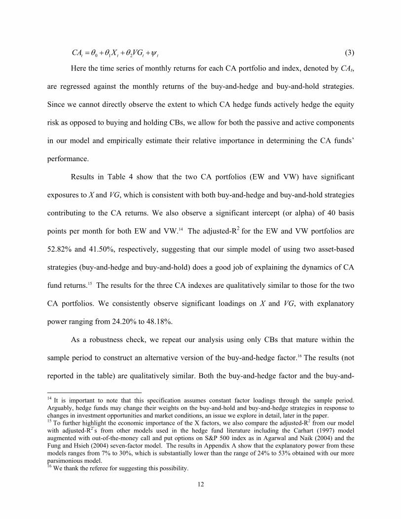
0 1 2t t t tCA X VG (3)

Here the time series of monthly returns for each CA portfolio and index, denoted by CAt,

are regressed against the monthly returns of the buy-and-hedge and buy-and-hold strategies.

Since we cannot directly observe the extent to which CA hedge funds actively hedge the equity

risk as opposed to buying and holding CBs, we allow for both the passive and active components

in our model and empirically estimate their relative importance in determining the CA funds’

performance.

Results in Table 4 show that the two CA portfolios (EW and VW) have significant

exposures to X and VG, which is consistent with both buy-and-hedge and buy-and-hold strategies

contributing to the CA returns. We also observe a significant intercept (or alpha) of 40 basis

points per month for both EW and VW.14 The adjusted-R2 for the EW and VW portfolios are

52.82% and 41.50%, respectively, suggesting that our simple model of using two asset-based

strategies (buy-and-hedge and buy-and-hold) does a good job of explaining the dynamics of CA

fund returns.15 The results for the three CA indexes are qualitatively similar to those for the two

CA portfolios. We consistently observe significant loadings on X and VG, with explanatory

power ranging from 24.20% to 48.18%.

As a robustness check, we repeat our analysis using only CBs that mature within the

sample period to construct an alternative version of the buy-and-hedge factor.16 The results (not

reported in the table) are qualitatively similar. Both the buy-and-hedge factor and the buy-and-

14 It is important to note that this specification assumes constant factor loadings through the sample period. Arguably, hedge funds may change their weights on the buy-and-hold and buy-and-hedge strategies in response to changes in investment opportunities and market conditions, an issue we explore in detail, later in the paper. 15 To further highlight the economic importance of the X factors, we also compare the adjusted-R2 from our model with adjusted-R2’s from other models used in the hedge fund literature including the Carhart (1997) model augmented with out-of-the-money call and put options on S&P 500 index as in Agarwal and Naik (2004) and the Fung and Hsieh (2004) seven-factor model. The results in Appendix A show that the explanatory power from these models ranges from 7% to 30%, which is substantially lower than the range of 24% to 53% obtained with our more parsimonious model. 16 We thank the referee for suggesting this possibility.

13

hold factor continue to be positively related to CA returns; the coefficient of the buy-and-hedge

factor is statistically significant in all cases but one and the coefficient of VG is always

statistically significant. The two-factor model produces adjusted R-squares ranging from 11% to

39% but lower than those reported in Table 4. This suggests that the buy-and-hedge factor that

uses all CBs does a better job of explaining CA returns during our sample period.

Since CBs are also exposed to interest rate risk and credit risk, in theory, CA funds may

also hedge these two risks in addition to the equity risk. However, the extent to which they do so

in practice must depend on the costs and benefits of hedging these risks which is an empirical

question. To answer this question, we repeat our analysis using an alternative buy-and-hedge

factor, XA, which hedges all three sources of risk (interest, credit and equity). XA is constructed as

follows. Equity risk is captured in EQt, as in the case of factor X. The impact of credit risk

inherent in CBs is proxied by the daily change in the spread between the yields of Baa corporate

bonds and 10-year U.S. Treasury bonds. To incorporate the impact of interest rate risk, we use

the daily yield of 5-year U.S. Treasury bonds. 17 The risks of the portfolio of CBs are hedged

using the following regression model:

, 0 1 2 3CB t t t t tR EQ IR CRg g g g h= + + + + (4)

Here ,CB tR is the day t return on the issue-size-weighted portfolio of CBs, EQt is the day t return

on the issue-size-weighted portfolio of underlying stocks, tIR is the day t interest rate proxy, and

tCR is the day t credit risk proxy. The return to the strategy that hedges all three risks follows

that of a portfolio comprising a long position in the issue-size-weighted portfolio of CBs, a short

position in the issue-size-weighted portfolio of the corresponding stocks, a short position in

17 We obtain these from the Federal Reserve Board website and Datastream.

14

government bonds, and a short position in the spread between corporate and government bonds.18

The short quantities are obtained from the slope estimates in equation (4).

After adjusting for financing and transaction costs, the returns corresponding to hedging

the equity, credit, and interest rate risks are EQt - (DISCt – s), CRt – (DISCt – s), and IRt –

(DISCt – s) respectively. We denote these cost-adjusted returns by XEQt, XCRt, and XIRt. The

cost-adjusted returns from the alternative buy-and-hedge factor, XA, is given by

, 1 2 3ˆ ˆ ˆ( )A

t CB t t t t tX R DISC XEQ XIR XCR (5)

where AtX is day t return on following the convertible arbitrage strategy, ,( )CB t tR DISC is the

day t return on the bond portfolio adjusted for borrowing cost ( )tDISC associated with funding

the long position in the CB portfolio, and , ,t tXEQ XCR and tXIR are as defined above.

Table 5 reports the results from the regression model of equation (3), re-estimated using

VG and XA. We observe that the loadings on the two factors are similar to those in Table 4.

However, using the alternative buy-and-hedge factor lowers explanatory power across all CA

portfolios and indexes. For example, for the EW CA portfolio, the two-factor model with the

original buy-and-hedge factor (X) achieves an adjusted-R2 of 52.82%, but the two-factor model

with the alternative buy-and-hedge factor (XA) produces a lower adjusted-R2 of 43.68%. This

suggests that our specification of hedging equity risk alone is a better characterization of the buy-

and-hedge strategy used by CA hedge funds in practice. Therefore, in the following analyses, our

buy-and-hedge strategy involves taking a long position in CBs and delta hedging the equity risk.

18 The stocks in the stock portfolio receive the same weight as the corresponding CBs. The interest rate and credit variables are indexes. Hence, there is no weighting for these variables.

15

These empirical results suggest that CA hedge funds behave in a manner consistent with

that of an intermediary who provides funding to the CB issuers while acting as an equity-risk

transfer agent distributing risk from the CB to the equity market.

4.2. How does the supply of CBs affect convertible arbitrageurs?

Viewed as a funding and risk intermediary for CB issuers, a convertible arbitrageur’s

performance in month t should depend on the supply of new CB issues available for trading

month t, NIt . However, simply relying on CB issuance dates recorded in databases produces an

inaccurate measure of NIt as these bonds often trade in the “when-issued” (WI) market--which

exists between the announcement date of a new issue and ends on the issuance date that can be

several months hence.19 The existence of the WI market means that the profit/loss effect of a new

CB issue can enter into a CA fund’s performance well before the recorded issuance date of

newly issued CBs as WI CB positions are marked to market for accounting purposes. The

combination of when issued trading and a potentially long settlement period between

announcement and issuance dates give rise to a measurement problem if one uses issuance dates

to construct a supply proxy. In other words, NIt contains bonds with issuance dates in months t+1,

t+2, or beyond. Therefore, the first step to constructing an accurate proxy of CB supply is to

gauge how far in time CB deals are announced in advance of eventual issuance. To that end, we

randomly sample (without replacement) 100 CBs that are issued during our sample period and

manually collect the earliest announcement date from Factiva news search supplemented with

19 Chacko et al. (2005) study the determinants of liquidity in the US corporate bond market using a dataset of when-issued and secondary market trades. Nyborg and Sundaresan (1996), among others, study when-issued trading in the US Treasury market. In private correspondence, a Financial Industry Regulatory Authority (FINRA) representative confirms the existence of when-issued trading in convertible bonds.

16

searches on the SEC EDGAR database and Google.20 Ninety-three of the 100 randomly selected

bonds have complete information.

Table 6 displays the frequency distribution of the announcement month relative to the

issuance month. About two-thirds of the announcements are made in the same month as the

issuance month while the remaining announcements are made before the issuance month. In

particular, about 24% of the CB deals are announced one month before the issuance month and

another 6% are announced two months before. Of the two remaining CB issues, one is

announced four months before issuance while another is announced five months before issuance.

This distribution suggests that a reasonable proxy of NIt includes CBs with issuance dates in

months t+1 and t+2. Accordingly, we construct our month t supply variable, LDealt , as

LDealt = log(1 + CBt+1 + CBt+2) (6)

where log(.) is the natural logarithm function, and CBt+1 (CBt+2) is the number of CB issues with

issuance dates in month t+1 (t+2).21 To test whether supply conditions affect CA performance,

we estimate the following regression model:

1 2t t t t tCA X VG LDeala b b g c= + + + + (7)

where LDealt is the supply variable in month t and the other variables are as in equation (3).

Table 7 reports the results from applying equation (7) to the two CA portfolios and the

three CA indexes. The coefficients for X and VG with respect to the two CA portfolios, EW and

VW, remain positive and statistically significant. In addition, the new supply variable LDeal has

a positive and highly significant coefficient for both the portfolios. After accounting for supply

effects via the LDeal variable, both CA portfolios exhibit significant negative alphas. This is in

20 Our CB data set from Albourne Partners contains the issuance dates, but not the announcement dates. In unreported work, we find that the distribution of sampled bonds across years is similar to the distribution for the entire sample of 1,646 bonds. 21 For robustness, we repeat our tests using the logarithm of the number of CB issues in month t, and find our results to be qualitatively similar.

17

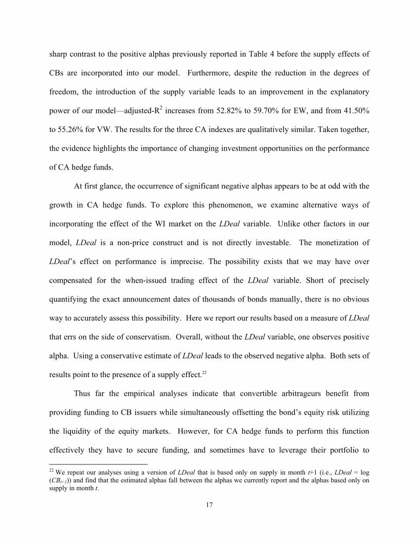
sharp contrast to the positive alphas previously reported in Table 4 before the supply effects of

CBs are incorporated into our model. Furthermore, despite the reduction in the degrees of

freedom, the introduction of the supply variable leads to an improvement in the explanatory

power of our model—adjusted-R2 increases from 52.82% to 59.70% for EW, and from 41.50%

to 55.26% for VW. The results for the three CA indexes are qualitatively similar. Taken together,

the evidence highlights the importance of changing investment opportunities on the performance

of CA hedge funds.

At first glance, the occurrence of significant negative alphas appears to be at odd with the

growth in CA hedge funds. To explore this phenomenon, we examine alternative ways of

incorporating the effect of the WI market on the LDeal variable. Unlike other factors in our

model, LDeal is a non-price construct and is not directly investable. The monetization of

LDeal’s effect on performance is imprecise. The possibility exists that we may have over

compensated for the when-issued trading effect of the LDeal variable. Short of precisely

quantifying the exact announcement dates of thousands of bonds manually, there is no obvious

way to accurately assess this possibility. Here we report our results based on a measure of LDeal

that errs on the side of conservatism. Overall, without the LDeal variable, one observes positive

alpha. Using a conservative estimate of LDeal leads to the observed negative alpha. Both sets of

results point to the presence of a supply effect.22

Thus far the empirical analyses indicate that convertible arbitrageurs benefit from

providing funding to CB issuers while simultaneously offsetting the bond’s equity risk utilizing

the liquidity of the equity markets. However, for CA hedge funds to perform this function

effectively they have to secure funding, and sometimes have to leverage their portfolio to

22 We repeat our analyses using a version of LDeal that is based only on supply in month t+1 (i.e., LDeal = log (CBt+1)) and find that the estimated alphas fall between the alphas we currently report and the alphas based only on supply in month t.

18

purchase the CBs. The ability of CA hedge funds to borrow short-term capital from prime

brokers as well as to attract longer term capital from their investors will in turn depend on

prevailing liquidity conditions in the market place. In this context, the question arises as to how

convertible arbitrageurs respond to market upheavals that interrupt their ability to fund their

portfolios? To gain insight into this question, we examine how CA hedge funds manage extreme

events such as the LTCM crisis.

4.3. The impact of extreme market events on CA hedge funds

We investigate the effect of the LTCM event on CA fund returns by testing for structural

breaks to our model. Following Brown et al. (1975), we apply the CUSUM procedure and

confirm that the LTCM crisis indeed lead to consistent boundary violations across the two CA

portfolios and the three CA indexes. Similar to Fung and Hsieh (2004) and Fung et al. (2008),

we use the following structural break model to account for the LTCM crisis:

0 1 2 0 3 41( ) 2( )t t t t t t t tCA D X VG LDeal D X VG LDealw w w g w w w p k= + + + + + + + + (8)

Here the variables are as defined before in equations (3) and (7).

The results from this joint estimation are reported in Table 8. There is a general decline in

the exposure to the buy-and-hold strategy uniformly across the CA portfolios and indexes

compared to the results reported in Table 7. The coefficient on D1 x VG is smaller than that on

D2 x VG for EW, CISDM, and HFR at varying levels of statistical significance. For the two

AUM-weighted constructs, the VW portfolio and the CT index, post-LTCM exposure to the

directional factor, VG, appear to have weakened both in slope coefficient as well as statistical

significance. These results are broadly consistent with an increase in risk aversion post LTCM.

Collaborative evidence can be seen in post-LTCM increases in the exposures to the buy-and-

19

hedge factor across all cases. However, we can only confirm the statistical significance for all

the CA indexes but not for the CA portfolios (see the F-test results for D1 x X in the lower panel

of Table 8). In terms of the effect of CB supply on returns, the results are mixed. Both the CA

portfolios and indexes exhibit significant positive loading on the supply variable (LDeal) before

the LTCM crisis similar to the results reported in Table 7. However, post LTCM, the coefficient

on LDeal is positive but only weakly significant (at the 10% level) for EW. But the F-tests failed

to reject the null that LDeal has identical coefficients before and after the LTCM crisis, with the

exception of VW. Taken together, there seems to be a preponderance of evidence pointing

towards a decrease in risk appetite (or an increase in risk aversion) after the LTCM crisis.

However, the variability of the results across the two portfolios (EW and VW) and three indexes

(CISDM, CT, and HFR) indicate potential behavioral differences in the cross section of funds—

an issue we investigate in more detail in the next section.

Finally, in terms of explanatory power, there is a uniform increase in adjusted-R2

compared to the results in Table 7. For example, with CISDM as the dependent variable,

equation (8) produces an adjusted-R2 of 75.49%, which is substantially higher than the adjusted-

R2 in Table 7 (55.44%). More importantly, both the pre-LTCM and post-LTCM alphas are

either insignificantly different from zero or negative. Overall, these findings confirm a lack of

abnormal performance from CA funds on average, after adjusting for the changes in investment

opportunities and the structural changes arising from extreme market events such as the LTCM

crisis. The natural question that arises is whether these conclusions apply uniformly across the

funds in our sample. 23 This is the subject of the next section.

23 We thank the referee for directing us towards analyzing individual CA funds.

20

5. Individual fund level analyses

The empirical results in the previous section point to potential differences in return

characteristics between the small funds (weighted higher in the EW portfolio as well as indices

such as the HFR and CISDM) and the larger funds, which have greater weighting in the VW

portfolio and the CT index. To investigate these differences, we begin by identifying all CA

hedge funds with at least 24 months of data on returns and assets under management during our

sample period. We then compute the time-series average of the assets under management for

each fund to sort funds into size terciles (Small, Medium, and Large). This procedure yields 36

CA hedge funds in each tercile, for a total of 108 funds. Within each size tercile, we estimate

equation (7), the two-factor plus supply effect model, for each fund. The summary statistics of

the respective size terciles and regression results are reported in Table 9 Panel A.

The sample moments of returns reveal differences across size terciles. Larger funds

(Medium and Large terciles) appear to generate higher returns than small funds. The mean

(median) monthly excess return on the Large, Medium, and Small portfolio is 0.51%, 0.65%, and

0.39% (0.66%, 0.78% and 0.63%), respectively. The largest and smallest funds experience

greater performance variability than the medium funds. The Large and Small portfolios have

monthly standard deviations of 1.25% and 1.29%, respectively, while the Medium portfolio has a

monthly standard deviation of 1.05%. Higher performance variability implies more extreme

returns that can create greater divergence between the mean and median. We do observe such a

pattern in the data. The Small and Large portfolios, with higher standard deviations, exhibit

larger differences between mean and median returns than the Medium portfolio. In terms of

Sharpe ratio, the Medium portfolio has the highest Sharpe ratio (0.62) while the Small portfolio

has the lowest Sharpe ratio (0.30).

21

Turning to the regression results, we see that the average coefficient of X is positive and

statistically significant at the 1% level, indicating that the buy-and-hedge factor continues to be a

significant explanatory variable among CA hedge funds of varying sizes. The average coefficient

of VG is positive and statistically significant for the small and medium terciles but not for larger

CA hedge funds. The average coefficient of LDeal is positive for all terciles, but is statistically

significant only for the medium and large terciles, suggesting that the supply variable is more

important in explaining the returns of medium and large funds. These findings are consistent

with larger funds being less dependent on security selection to support performance for their

capital base. This observation is, in turn, consistent with a diseconomy of scale to skill-based

investment strategies resulting in larger funds being more dependent on systematic, factor-related

returns for performance. Consequently, declines in the supply of convertible bonds are likely to

negatively impact them more than their smaller brethren. Consistent with the results in Table 7,

the non-factor related returns from this three-factor model are not statistically different from zero

for smaller funds and negative for medium and larger funds. However the model’s explanatory

power, adjusted R2, for each of the three terciles is notably lower than those reported for the

broader averages in Table 7.

Next, we examine how well the structural break model explains fund returns across the

size terciles. For this analysis, we apply a different selection procedure to ensure that the funds

selected have a sufficiently long return history that spans the LTCM crisis. Specifically, we only

include CA hedge funds with at least 48 months of data on returns and assets under management

during our sample period to ensure sufficient degrees of freedom for efficient estimation. In

addition, the funds must have existed before, during, and after the LTCM crisis. In other words,

the return series must span the LTCM crisis. This second condition ensures that D1 and D2, as

22

well as all associated interaction terms can be estimated for each fund. The selection procedure

yields 15 CA hedge funds for each size tercile. 24 Panel B of Table 9 reports the average

regression coefficients, adjusted-R2, and fund characteristics. Because our selection procedure

yields a subset of the original size terciles (employed in Table 9 Panel A), we also report

summary statistics of monthly excess returns on these new size terciles. To summarize tests of

differences of coefficients among the funds, we report the number of funds for which there is a

statistically significant increase or decrease in coefficient after the LTCM crisis.25

In terms of sample moments of returns, we continue to observe similar patterns to the

results in Table 9 Panel A. Specifically, larger funds (Medium and Large terciles) appear to

generate higher returns than small funds. For example, the median monthly excess return on the

Large, Medium, and Small portfolio is 0.77%, 0.67%, and 0.54%, respectively. Performance

variability is higher among the largest and smallest funds than among the midsize funds; the

Large (Small) portfolio has a monthly standard deviation of 2.12% (1.25%) while the Medium

portfolio has a monthly standard deviation of 0.91%. As expected, greater return variability in

the Large and Small portfolios result in more pronounced differences between mean and median

returns. The Medium portfolio has the highest Sharpe ratio (0.69) and the Large portfolio has the

lowest (0.23).

The fund-level regression results add clarity to those of CA indexes and portfolios in

several respects. First, they clarify that the exposure to the directional variable, VG, reported in

Table 8 for the broad-based portfolios and indexes are primarily driven by the smaller funds.

24 In unreported work, we compute the grand average age for each size tercile and find no systematic relation between size and age. Grand average age (in years) in the Small, Medium, and Large tercile is 5.7, 4.1, and 4.4, respectively. There is no apparent age bias in the terciles. Interestingly, the higher age of small funds is consistent with their greater survival rate and less negative abnormal performance based on the results in Table 9 Panel A. 25 We identify a change in coefficient as statistically significant if the F-statistic implies a rejection of the null of no change at the 10% level or lower.

23

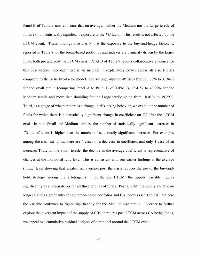
Panel B of Table 9 now confirms that on average, neither the Medium nor the Large tercile of

funds exhibit statistically significant exposure to the VG factor. This result is not affected by the

LTCM event. These findings also clarify that the exposure to the buy-and-hedge factor, X,

reported in Table 8 for the broad-based portfolios and indexes are primarily driven by the larger

funds both pre and post the LTCM crisis. Panel B of Table 9 reports collaborative evidence for

this observation. Second, there is an increase in explanatory power across all size terciles

compared to the basic two-factor model. The average adjusted-R2 rises from 23.60% to 31.84%

for the small tercile (comparing Panel A to Panel B of Table 9), 25.41% to 43.99% for the

Medium tercile and more than doubling for the Large tercile going from 18.01% to 39.29%.

Third, as a gauge of whether there is a change in risk-taking behavior, we examine the number of

funds for which there is a statistically significant change in coefficient on VG after the LTCM

crisis. In both Small and Medium terciles, the number of statistically significant decreases in

VG’s coefficient is higher than the number of statistically significant increases. For example,

among the smallest funds, there are 4 cases of a decrease in coefficient and only 1 case of an

increase. Thus, for the Small tercile, the decline in the average coefficient is representative of

changes at the individual fund level. This is consistent with our earlier findings at the average

(index) level showing that greater risk aversion post the crisis reduces the use of the buy-and-

hold strategy among the arbitrageurs. Fourth, pre LTCM, the supply variable figures

significantly as a return driver for all three terciles of funds. Post LTCM, the supply variable no

longer figures significantly for the broad-based portfolios and CA indexes (see Table 8), but here

the variable continues to figure significantly for the Medium size tercile. In order to further

explore the divergent impact of the supply of CBs on returns post LTCM across CA hedge funds,

we appeal to a cumulative residual analysis of our model around the LTCM event.

24

For each tercile, we first estimate equation (8) without the LDeal variable for each fund

and use the factor loadings to compute each fund’s monthly residuals. Specifically, in the period

prior to and including the LTCM month (from March 1998 to September 1998), fund i’s residual

in month t, Residuali,t, is the difference between its excess return and the product of the pre-

LTCM factor loadings and factor realizations, i.e.,

Residuali,t = CAi,t − (d1Xi x Xt + d1VGi x VGt) (9)

where CAi,t is fund i’s excess return in month t, d1Xi (d1VGi) is fund i’s pre-LTCM coefficient

on X (VG), and Xt (VGt) is the buy-and-hedge (buy-and-hold) factor realization in month t.

Similarly, for the 10 months after LTCM (from October 1998 to July 1999)26, Residuali,t is

computed as the difference between its excess return and the product of the post-LTCM factor

loadings and factor realizations.

Residuali,t = CAi,t − (d2Xi x Xt + d2VGi x VGt) (10)

where CAi,t is fund i’s excess return in month t, d2Xi (d2VGi) is fund i’s post-LTCM coefficient

on X (VG), and Xt (VGt) is the buy-and-hedge (buy-and-hold) factor realization in month t.

Next we average the fund level residuals across funds each month to obtain the equally-

weighted residual for each tercile. We then cumulate the equally-weighted residuals to obtain

cumulative residuals for each tercile. In Figure 1, we plot the cumulative residuals for the size

terciles from March 1998 to July 1999. The cumulative residual plots show that all three groups

appear to have recovered from the LTCM event, albeit at varying speeds, by the middle of 1999.

Accompanying the residual plots is the plot of cumulative CB issuance (‘cumulative

supply’), which shows that CB issuance dropped dramatically during the crisis (the flat portion

26 In July 1999, 12 CBs were issued, a number that is comparable to the pre-LTCM issuance of 13 CBs in July 1998 and 12 CBs in August 1998. Thus, we choose to end the post-LTCM period in July 1999 to examine whether the recovery of CB supply to approximately pre-LTCM levels has differential impact on fund performance after the LTCM crisis.

25

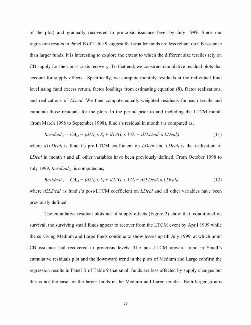
of the plot) and gradually recovered to pre-crisis issuance level by July 1999. Since our

regression results in Panel B of Table 9 suggest that smaller funds are less reliant on CB issuance

than larger funds, it is interesting to explore the extent to which the different size terciles rely on

CB supply for their post-crisis recovery. To that end, we construct cumulative residual plots that

account for supply effects. Specifically, we compute monthly residuals at the individual fund

level using fund excess return, factor loadings from estimating equation (8), factor realizations,

and realizations of LDeal. We then compute equally-weighted residuals for each tercile and

cumulate those residuals for the plots. In the period prior to and including the LTCM month

(from March 1998 to September 1998), fund i’s residual in month t is computed as,

Residuali,t = CAi,t − (d1Xi x Xt + d1VGi x VGt + d1LDeali x LDealt) (11)

where d1LDeali is fund i’s pre-LTCM coefficient on LDeal and LDealt is the realization of

LDeal in month t and all other variables have been previously defined. From October 1998 to

July 1999, Residuali,t is computed as,

Residuali,t = CAi,t − (d2Xi x Xt + d2VGi x VGt + d2LDeali x LDealt) (12)

where d2LDeali is fund i’s post-LTCM coefficient on LDeal and all other variables have been

previously defined.

The cumulative residual plots net of supply effects (Figure 2) show that, conditional on

survival, the surviving small funds appear to recover from the LTCM event by April 1999 while

the surviving Medium and Large funds continue to show losses up till July 1999, at which point

CB issuance had recovered to pre-crisis levels. The post-LTCM upward trend in Small’s

cumulative residuals plot and the downward trend in the plots of Medium and Large confirm the

regression results in Panel B of Table 9 that small funds are less affected by supply changes but

this is not the case for the larger funds in the Medium and Large terciles. Both larger groups

26

depend on new CB issues without which, the cumulative residual continues to decline,

suggesting little or no recovery of losses on non-factor related return from the LTCM event itself.

Overall, our analysis at the individual fund level reveals substantial cross-sectional

variation in the use of buy-and-hedge strategy relative to the buy-and-hold strategy, and the

impact of supply and market conditions on the abnormal performance of CA funds. As the

description of CA hedge funds suggests, there is a growing (as measured in the assets under

management) dependence on hedged convertibles bonds as a strategy for larger funds. In

contrast, smaller CA hedge funds are more dependent on the directional performance of CBs and

less reliant on hedging. Consequently when a major market upheaval such as the LTCM crisis

comes along, the surviving small funds are able to reap the benefits sifting through the wreckage

left behind from funds that had to deleverage or were liquidated entirely. For larger funds,

security selection is not the main performance driver given their bigger capital base and their

dependence on hedged convertibles, factor X, as a strategy. Pre and post a major market crisis

such as LTCM, any loss due to deleveraging appears to be almost permanent or at least to take a

much longer time to recoup (judging by the cumulative residual analysis) compared to their

smaller, more nimble, brethrens that survived. As such, marginal increases/decreases in the

supply of bonds would appear less relevant to their long-term performance. In contrast, the

Medium size funds continue to exhibit, pre and post LTCM, consistent exposures to the buy-and-

hedge factor as well as being performance reliant on the supply of CBs. Thus far, these

empirical conclusions are based on data from hedge funds and CBs over two five-year periods

surrounding the LTCM event. The natural question to ask is whether the return drivers we have

identified continue to be the key determinants of CA investors’ portfolios.

27

6. Out-of-sample analysis of funded CA portfolios

6.1. Construction of the variables for the out-of-sample period

In this section we focus on an out-of-sample period between May 2003 and June 2007.

During this period, investable versions of the CA indexes from CT and HFR (“CTX” and

“HFRX” for short) were launched and had successfully attracted investors’ capital. These

products are designed to offer investors a broad exposure to CA hedge funds with explicitly

defined, rule-based portfolio constructions. As such, they inherit all the trading frictions of a

real-life CA hedge fund portfolio bringing in some of the practical considerations that are

typically assumed away in statistical indexes.27

For consistency, we adjusted the two return factors to better reflect the trading friction of

the dependent variables. In terms of the buy-and-hold factor, VG, is available and remained open

as a mutual fund throughout the out-of-sample period. To proxy an investable version of the

buy-and-hedge factor, X, we employ an alternative approach. We use VG to proxy the long-CB

component of the buy-and-hedge factor. To estimate the hedge ratio for the short-equity

component, we regress VG on the Russell 2000 index:

0 1t t tVG RUS v (13)

where RUSt is the month t return on the Russell 2000 index.28 To obtain the equity hedge ratio for

month t, we perform an OLS estimation of equation (13) using data from the previous 24 months.

The slope coefficient estimate for RUSt, 1̂ , serves as the equity hedge ratio for month t. We then

compute the buy-and-hedge factor in month t as:

27 Practical considerations include issues such as whether a fund is open to new investors, the friction involved in rebalancing a portfolio with funds that stipulate different redemption terms and free of survivorship biases that may exist in indexes of hedge funds—see Fung and Hsieh (2004) for discussions of these issues. 28 Both ETFs and Futures Contract on the Russell 2000 exist and closely track the index. However, to ensure we match the data period in our analysis with the investable hedge fund indices and to avoid basis considerations that may arise from the futures contract, we opted to use the index return series instead.

28

, 1̂O t t tX VG RUS (14)

A rolling 24-month window is used to repeat the two-step procedure. In particular, we use the

monthly returns on VG and RUS from May 2001 to June 2007 with the first (last) estimation

window corresponding to May 2001 to April 2003 (June 2005 to May 2007).29 Table 10 Panel A

shows that the CA indexes have average monthly returns ranging from −0.12% to 0.21% in the

out-of-sample period. The negative average return corresponds to HFRX while all other indexes

have positive average returns. Median returns portray a similar picture: CISDM, CT, CTX, and

HFR indexes all have higher medians than HFRX. In terms of dispersion, CISDM, CTX, and

HFR exhibit lower volatility compared to CT and HFRX. Overall, there are discernable

differences between indexes, which are primarily statistical constructs, and the investable

portfolios. Consistent with the pattern observed in-sample, Table 10 Panel B shows that the CA

indexes are highly correlated with each other while VG and OX continue to exhibit strong

positive correlations with the CA indexes.

6.2. Out-of-sample analysis with the buy-and-hedge and buy-and-hold factors

To verify that the investable factors OX and VG continue to be significant determinants of

CA hedge funds in the out-of-sample period, we regress CA index returns on OX and VG:

0 1 , 2t O t t tCA X VG

(15)

The results are reported in Table 11. The coefficients of XO and VG are positive and highly

significant for all CA indexes with adjusted-R2 ranging from 41.08% to 44.93%. 29 To illustrate that the out-of-sample version of the X factor is similar to the in-sample version, we repeat the regression in equation (3) with the out-of-sample version and report the results in Appendix B. We find that the results are similar to those in Table 4 with the X factor continuing to be significant in all cases and the explanatory power ranging from 15% to 37%, which is lower than the range of 24% to 53% obtained earlier with the in-sample version. This is to be expected as the out-of-sample version of the X factor is unlikely to be as precise as the in-sample version, which is created by delta-hedging the portfolio of individual stocks corresponding to the different CBs as opposed to delta-hedging the Russell 2000 index. Considering the lack of data on individual CBs during the out-of-sample period, we believe this is the best proxy we can construct.

29

During our sample period from January 1993 to April 2003, we use the non-investable

convertible arbitrage indexes as their investable counterparts are not available. However, during the

out-of-sample period from May 2003 to June 2007, we notice and recognize the introduction of

investable indexes. Hence, as a sensitivity check, we repeat our analysis with the investable indexes.

Both HFR indexes (HFR and HFRX) load positively and significantly on the buy-and-hold and buy-

and-hedge factors, which is consistent with HFR’s objective of constructing an investable index that

has maximum correlation with its investable counterpart. In contrast, regression results for the CS

Tremont indices do diverge in one respect. While the non-investable index, CT, has positive and

significant loadings on the buy-and-hold and buy-and-hedge factors, its investable counterpart, CTX,

only shows a positively significant exposure to the buy-and-hold factor. The coefficient on the buy-

and-hedge factor is positive, but has a t-statistic of 1.67 (p-value of 0.102). One possible explanation

for the slight loss of statistical power is the fact CTX has a somewhat shorter return history than CT

during the out-of-sample period; CT has 50 monthly observations whereas CTX has 47 monthly

observations.30 It is interesting to note that when we augment the two-factor model with the supply

variable (see Table 12), both CT and CTX have positive and statistically significant loadings on the

buy-and-hold and buy-and-hedge factors.

Next we examine the effect of CB supply on performance.

6.3. Out-of-sample analysis with the buy-and-hedge and buy-and-hold factors along with the

supply variable

The supply variable, LDeal, used in the sample period is constructed from individual CB

data, which end in April 2003. To construct the same variables for the out-of-sample period, we

30 Another possible explanation is that CT and CTX have different construction methodologies, resulting in different constituent funds in each index and divergent return properties. CT is a value-weighted index of CA hedge funds while CTX is a value-weighted index of the six largest eligible funds making up CT. However, Table 10 Panel B shows that both indices have a high correlation of 0.95, suggesting that index construction is a less likely explanation.

30

collect CB issuance data from Thomson Reuters Financial’s SDC Platinum database. To validate

our choice and verify the consistency between the Albourne and SDC databases, we compare

monthly CB issuance from the individual CB data from Albourne Partners with that from SDC

during the sample period (January 1993 to April 2003). We find that both variables are closely

matched in terms of sample moments and are highly correlated.31 This provides us comfort in

using the supply variable constructed from the SDC data to estimate the following regression in

the out-of-sample period:

1 2t t t t tCA X VG LDeal (16)

The regression results in Table 12 indicate significant loadings on the buy-and-hedge

factor across all non-investable CA indexes, corroborating our in-sample results. There is a

notable increase in the explanatory power of our model. The adjusted-R2 now ranges from

48.72% to 56.44% (compared to 41.08% to 44.93% in Table 11), which underscores the

importance of accounting for supply variable in explaining the returns of CA strategy.

Interestingly, the relevance of the buy-and-hold factor has weakened in the out-of-sample period.

Supply effects continue to play an important role in explaining CA index returns during the out-

of-sample period; the coefficient on LDeal is positive and significant for all CA indexes.

Consistent with the earlier evidence of supply effects explaining the abnormal returns, we

observe that all alphas are now significantly negative. In terms of the investable indexes, the

supply variable figures significantly in the regression model and exhibits positive loadings.

Including the supply variable enhances the explanatory power of the model. Exposures to the

investable buy-and-hedge and buy-and-hold factors remain similar. There is, however, a notable

increase in both the magnitude as well as statistical significance of the negative alpha term. 31 The summary statistics (mean, median, minimum, maximum, and the standard deviation) of the number of deals per month in the US are 13.3, 12.0, 1.0, 48.0, and 8.3 using Albourne data. The corresponding figures are 11.6, 11.0, 1.0, 41.0, and 6.6 for SDC. The correlation between the two series is 0.76.

31

Overall, these out-of-sample analyses using investable CA portfolios and factors confirm

the earlier findings. Taken together, they show that our model can be used to capture the risk-

return characteristics of investing in CA funds in a real-life setting.

7. Conclusion

In this paper, we provide a rare glimpse into the strategies used by convertible

arbitrageurs. We posit that these arbitrageurs assume the role of an intermediary that provides

capital to the CB issuers while transmitting the equity risk of CB ownership to the equity market

through delta hedging. Using daily data from the underlying convertible bond and stock markets

in the US, we compute the returns to a buy-and-hedge strategy, which involves taking a long

position in the convertible bonds and hedging the equity risk by shorting the shares of CB issuers.

We show that such a strategy together with a simple buy-and-hold strategy can explain a large

proportion of the return variation in convertible arbitrage hedge funds. In addition, our results

reveal the important role played by supply conditions in determining the returns of convertible

arbitrage hedge funds. Furthermore, we show that convertible arbitrageurs are sensitive to

extreme market events such as the LTCM crisis. In response to such events, we demonstrate that

there can be an increase in the risk aversion of economic agents, which results in less reliance on

the buy-and-hold strategy. Examining the returns of individual convertible arbitrage funds

uncovers interesting cross-sectional variation in the use of buy-and-hedge strategy and the

impact of CB supply. Larger funds tend to rely more on the buy-and-hedge strategy and exhibit

less directional exposure to CBs, which is consistent with the economies of scale they enjoy in

accessing the stock loan market. Large funds also are more vulnerable to supply shocks, which is

suggestive of frictions involved in adjusting the stock of risk capital in response to the decline in

32

CB supply. Finally, out-of-sample analysis using investable CA portfolios and factors confirm

that our key findings persist in more recent times as well as with real-life portfolios.

Taken together, these results suggest that convertible arbitrageurs collectively play the

role of an intermediary who provides funding to convertible bond issuers whilst transferring the

equity risk of CB ownership to the equity market through hedging. This conclusion appears to

be robust to sample periods as well as the frictions of investing in CA funds.

33

Acknowledgements We are grateful to the following for their comments: Viral Acharya, George Aragon, Vladamir

Atanasov, Nicole Boyson, James Dow, Mark Hutchinson, Jeremy Large, Tobias Moskowitz,

Melvyn Teo, Heather Tookes, David Vang, Kumar Venkataraman, Sriram Villuparam, Tao Wu,

an anonymous referee and the participants at the European Financial Association meetings,

European Winter Finance conference 2007, FMA 2006 meetings, FMA European meetings,

London School of Economics conference on “Risk and Return Characteristics of Hedge Funds”,

Man Group, and Second Annual Asset Pricing Retreat. An earlier version of this paper was

adjudged the best paper on hedge funds at the European Finance Association (EFA) 2006

meetings. We are grateful for funding from INQUIRE Europe and support from BNP Paribas

Hedge Fund Centre at the London Business School. Vikas is grateful for the research support in

form of a research grant from the Robinson College of Business of Georgia State University. We

are thankful to Burak Ciceksever and Kari Sigurdsson for excellent research assistance. We

thank Albourne Partners, London for providing us the daily data on convertible bonds and

underlying stocks. We are responsible for all errors.

34

References

Agarwal, V., Naik, N.Y., 2004. Risks and portfolio decisions involving hedge funds. Rev. Finan.

Stud. 17, 63–98.

Agarwal, V., Daniel, N.D., Naik, N.Y., 2009. Role of managerial incentives and discretion in

hedge fund performance. J. Financ. 64, 2221–2256.

Almazán, A., Brown, K.C., Carlson, M., Chapman, D.A., 2004. Why constrain your mutual fund

manager? J. Financ. Econ. 73, 289–321.

Brennan, M.J., Kraus, A., 1987. Efficient financing under asymmetric information. J. Financ. 42,

1225–1243.

Brennan, M.J., Schwartz, E.S., 1977. Convertible bonds: Valuation and optimal strategies for

call and conversion. J. Financ. 32, 1699–1715.

Brennan, M.J., Schwartz, E.S., 1980. Analyzing convertible bonds. J. Financ. Quant. Anal. 15,

907–929.

Brennan, M.J., Schwartz, E.S., 1988. The case for convertibles. J. Appl. Corp. Financ. 1, 55–64.

Brown, R.L., Durbin, J., Evans, J.M., 1975. Techniques for testing the constancy of regression

relationships over time. J. Royal Stat. Soc. Series B (Methodological) 37, 149–192.

Brown, S.J., Grundy, B.D., Lewis, C.M., Verwijmeren, P., 2010. Convertibles and hedge funds

as distributors of equity exposure. Working Paper. New York University.

Buchan, J., 1997. Convertible bond pricing: theory and evidence. Unpublished Dissertation.

Harvard University.

Carhart, M., 1997. On persistence in mutual fund performance. J. Financ. 52, 57–82.

35

Chacko, G., Mahanti, S., Malik, G., Subrahmanyam, M.G., 2005. The determinants of liquidity

in the corporate bond markets: An application of latent liquidity. Working Paper. New York

University.

Chan, A.W.H., Chen, N., 2007. Convertible bond underpricing: Renegotiable covenants,

seasoning, and convergence. Manag. Sci. 53, 1793–1814.

Choi, D., Getmansky, M., Tookes, H., 2009. Convertible bond arbitrage, liquidity externalities,

and stock prices. J. Financ. Econ. 91, 227–251.

Choi, D., Getmansky, M., Henderson, B., Tookes, H., 2010. Convertible bond arbitrageurs as

suppliers of capital, Rev. Finan. Stud. 23, 2492-2522.

Constantinides, G.M., Grundy, B.D., 1989. Optimal investment with stock repurchase and

financing as signals. Rev. Finan. Stud. 2, 445–465.

Das, S.R., Sundaram, R.K., 2004. A simple model for pricing securities with equity, interest rate

and default risk. Working Paper. New York University.

Davis, M., Lischka, F.R., 1999. Convertible bonds with market risk and credit risk. Working

Paper. Tokyo-Mitsubishi International PLC.

Duarte, J., Longstaff, F.A., Yu, F., 2007. Risk and return in fixed income arbitrage: Nickels in

front of a steamroller. Rev. Finan. Stud. 20, 769–811.

Fama, E.F., French, K.R., 1993. Common risk factors in the returns on stocks and bonds. J.

Financ. Econ. 33, 3–56.

Fung, W., Hsieh, D.A., 1997. Empirical characteristics of dynamic trading strategies: The case of

hedge funds. Rev. Finan. Stud. 10, 275–302.

Fung, W., Hsieh, D.A., 2001. The risk in hedge fund strategies: Theory and evidence from trend

followers. Rev. Finan. Stud. 14, 313–341.

36

Fung, W., Hsieh, D.A., 2004. Hedge fund benchmarks: A risk based approach. Financ. Anal. J.

60, 65–80.

Fung, W., Hsieh, D.A., Naik, N.Y., Ramadorai, T., 2008. Hedge funds: Performance, risk, and

capital formation. J. Financ. 63, 1777–1803.

Gatev, E.G., Goetzmann, W.N., Rouwenhorst, K.G., 2006. Pairs trading: Performance of a

relative-value arbitrage rule. Rev. Finan. Stud. 19, 797–827.

Goetzmann, W.N., Ingersoll, J., Ross, S.A., 2003. High-water marks and hedge fund

management contracts. J. Financ. 58, 1685–1718.

Green, R., 1984. Investment incentives, debt and warrants. J. Financ. Econ. 13, 115–136.

Gupta, A., Liang, B., 2005. Do hedge funds have enough capital? A value-at-risk approach. J.

Financ. Econ. 77, 219–253.

Ingersoll, J., 1977. A contingent-claims valuation of convertible securities. J. Financ. Econ. 4,

289–321.

Jensen, M.C., Meckling, W.H., 1976. Theory of the firm: managerial behavior, agency costs and

ownership structure. J. Financ. Econ. 3, 305–360.

Mayers, D., 1998. Why firms issue convertible bonds: The matching of financial and real

investment options. J. Financ. Econ. 47, 83–102.

McConnell, J.J., Schwartz, E.S., 1986. LYON Taming. J. Financ. 41, 561–576.

Merton, R.C., 1973. An intertemporal capital asset pricing model. Econometrica 41, 867–887.

Mitchell, M., Pedersen, L.H., Pulvino, T., 2007. Slow moving capital. Am. Econ. Rev. 97, 215–

220.

Mitchell, M., Pulvino, T., 2001. Characteristics of risk in risk arbitrage. J. Financ. 56, 2135–2175.

37

Newey, W., West, K., 1987. A simple, positive semi-definite, heteroskedasticity and

autocorrelation consistent covariance matrix. Econometrica 55, 703–708.

Nyborg, K., Sundaresan, S., 1996. Discriminatory versus uniform treasury auctions: Evidence

from when-issued transactions. J. Financ. Econ. 42, 63–105.

Pulliam, S., 2004. Mixed blessing: How hedge-fund trading sent a company's stock on wild ride.

Wall Street Journal December 28, A1.

Stein, J.C., 1992. Convertible bonds as backdoor equity financing. J. Financ. Econ. 32, 3–21.

Tsiveriotis, K., Fernandes, C., 1998. Valuing convertible bonds with credit risk. J. Fixed Income

8, 95–102.

Woodson, H., 2002. Global convertible investing : The Gabelli way. Wiley, New York.

Zuckerman, G., 2008. Convertible bonds cause hedge funds serious pain. Wall Street Journal

November 4, C1.

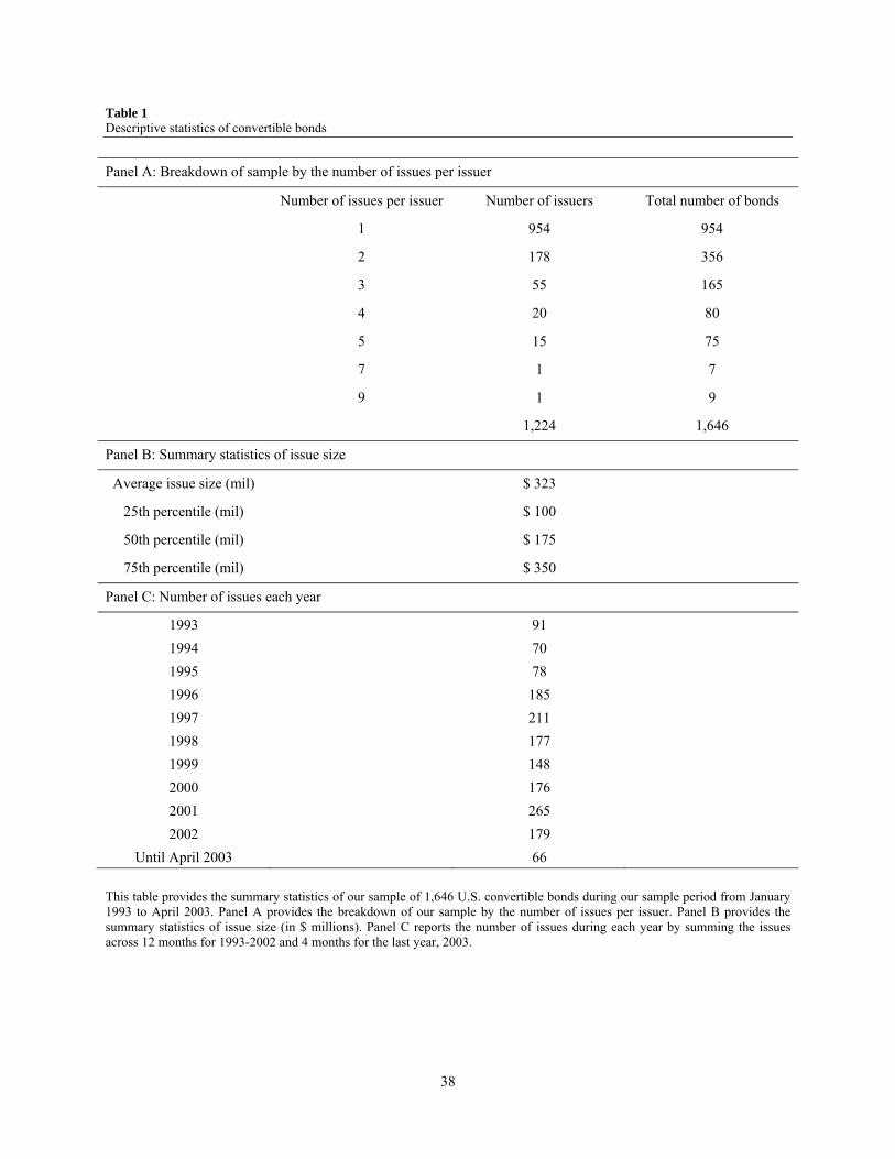
38

Table 1 Descriptive statistics of convertible bonds

Panel A: Breakdown of sample by the number of issues per issuer

Number of issues per issuer Number of issuers Total number of bonds

1 954 954

2 178 356

3 55 165

4 20 80

5 15 75

7 1 7

9 1 9

1,224 1,646

Panel B: Summary statistics of issue size

Average issue size (mil) $ 323

25th percentile (mil) $ 100

50th percentile (mil) $ 175

75th percentile (mil) $ 350

Panel C: Number of issues each year

1993 91 1994 70 1995 78 1996 185 1997 211 1998 177 1999 148 2000 176 2001 265 2002 179

Until April 2003 66

This table provides the summary statistics of our sample of 1,646 U.S. convertible bonds during our sample period from January 1993 to April 2003. Panel A provides the breakdown of our sample by the number of issues per issuer. Panel B provides the summary statistics of issue size (in $ millions). Panel C reports the number of issues during each year by summing the issues across 12 months for 1993-2002 and 4 months for the last year, 2003.

39

Table 2 Descriptive statistics of the buy-and-hedge factor

Panel A: Bonds used to construct X factor

Average number of bonds 411

Current yield (%) 13

Parity (%) 69

Age of bonds (in years) 2.4

Panel B: Summary statistics of the monthly returns of X factor

Mean (%) 0.17

Median (%) 0.22

SD (%) 1.01

Min. (%) -1.78

Max. (%) 1.95

Skew -0.14

Kurt -0.48

We report descriptive statistics of the buy-and-hedge factor, X. Panel A provides the daily average of the number of convertible bonds, current yield, parity, and age of convertible bonds in the portfolio generating the X factor. Current yield is computed using a full year's coupon divided by the bond's price (which incorporates accrued interest). Parity is the bond's conversion value as a percentage of the par value. Age is the number of years since the bond was issued. Panel B provides summary statistics of the buy-and-hedge factor’s monthly returns during our sample period from January 1993 to April 2003.

40

Table 3 Descriptive statistics of the long-biased convertible bond portfolio and the convertible arbitrage portfolios

Panel A: Summary Statistics

Mean (%) Median (%) SD (%) Min. (%) Max. (%) Skew Kurt VG 0.32 0.22 3.72 -13.25 10.11 -0.43 1.33

EW 0.56 0.68 1.03 -4.00 2.55 -1.08 2.51 VW 0.50 0.74 1.28 -4.66 3.04 -1.24 2.59

CISDM 0.61 0.74 0.67 -2.35 2.20 -1.36 3.98

CT 0.47 0.79 1.38 -5.10 3.07 -1.69 4.55 HFR 0.57 0.71 0.98 -3.65 2.93 -1.39 3.99

Panel B: Correlations between VG, the two CA portfolios, the three CA indexes and the X factor

VG EW VW CISDM CT HFR X

VG 1.00

EW 0.60*** 1.00

VW 0.49*** 0.90*** 1.00

CISDM 0.55*** 0.92*** 0.83*** 1.00

CT 0.34*** 0.81*** 0.85*** 0.80*** 1.00

HFR 0.51*** 0.90*** 0.84*** 0.93*** 0.80*** 1.00

X 0.39*** 0.62*** 0.58*** 0.61*** 0.48*** 0.60*** 1.00

Panel A of this table provides the descriptive statistics of the monthly returns of the Vanguard Convertible Securities mutual fund (VG), equally-weighted and value-weighted portfolios of all CA hedge funds (EW and VW) and three convertible arbitrage (CA) indexes (CISDM, CT, and HFR) from January 1993 to April 2003 with the exception of the CT index, which starts in 1994. The descriptive statistics include mean, median, standard deviation (SD), minimum (Min.), maximum (Max.), skewness (Skew), and kurtosis (Kurt). Panel B provides the correlations among the above return series and the buy-and-hedge factor, X. *, **, and *** indicate that the coefficient is significantly different from zero at the 10, 5, and 1% levels respectively.

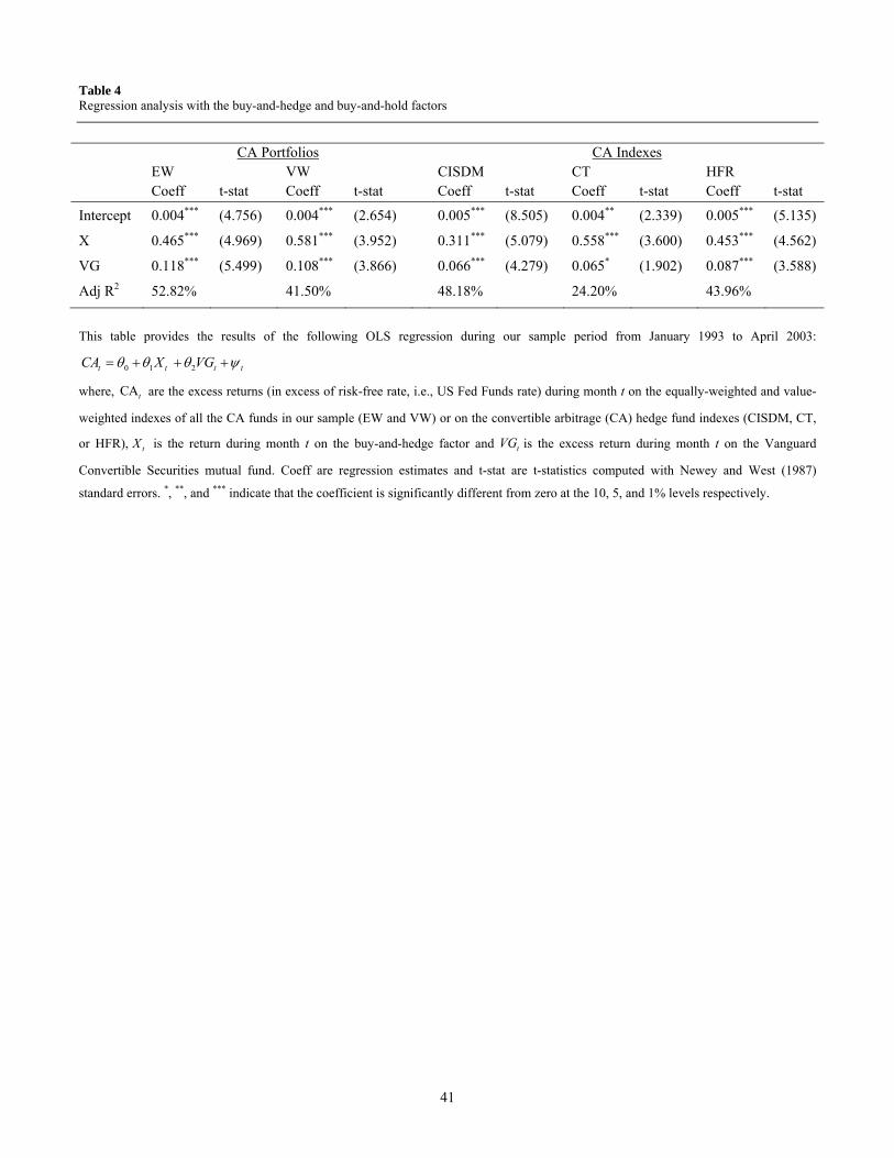
41

Table 4 Regression analysis with the buy-and-hedge and buy-and-hold factors

CA Portfolios CA Indexes EW VW CISDM CT HFR Coeff t-stat Coeff t-stat Coeff t-stat Coeff t-stat Coeff t-stat

Intercept 0.004*** (4.756) 0.004*** (2.654) 0.005*** (8.505) 0.004** (2.339) 0.005*** (5.135)

X 0.465*** (4.969) 0.581*** (3.952) 0.311*** (5.079) 0.558*** (3.600) 0.453*** (4.562)

VG 0.118*** (5.499) 0.108*** (3.866) 0.066*** (4.279) 0.065* (1.902) 0.087*** (3.588)

Adj R2 52.82% 41.50% 48.18% 24.20% 43.96%

This table provides the results of the following OLS regression during our sample period from January 1993 to April 2003:

0 1 2t t t tCA X VG

where, CAt are the excess returns (in excess of risk-free rate, i.e., US Fed Funds rate) during month t on the equally-weighted and value-

weighted indexes of all the CA funds in our sample (EW and VW) or on the convertible arbitrage (CA) hedge fund indexes (CISDM, CT,

or HFR), tX is the return during month t on the buy-and-hedge factor and tVG is the excess return during month t on the Vanguard

Convertible Securities mutual fund. Coeff are regression estimates and t-stat are t-statistics computed with Newey and West (1987)

standard errors. *, **, and *** indicate that the coefficient is significantly different from zero at the 10, 5, and 1% levels respectively.

42

Table 5 Results with the alternative buy-and-hedge factor, XA

CA Portfolios CA Indexes EW VW CISDM CT HFR Coeff t-stat Coeff t-stat Coeff t-stat Coeff t-stat Coeff t-stat

Intercept 0.003*** (2.884) 0.002 (1.327) 0.005*** (5.783) 0.003 (1.214) 0.004*** (2.961)

XA 0.345*** (3.886) 0.447*** (3.271) 0.226*** (3.915) 0.405*** (2.693) 0.361*** (4.036)

VG 0.115*** (4.281) 0.102*** (3.015) 0.065*** (3.385) 0.059 (1.423) 0.081*** (2.858)

Adj R2 43.68% 32.75% 38.05% 16.51% 35.73%

This table provides the results of the following OLS regression during our sample period from January 1993 to April 2003:

0 1 2CA VGAt t t tXh h h p= + + +

where, CAt are the excess returns (in excess of risk-free rate, i.e., US Fed Funds rate) during month t on the equally-weighted and value-

weighted indexes of all the CA funds in our sample (EW and VW) or on the convertible arbitrage (CA) hedge fund indexes (CISDM, CT, or HFR), A

tX is the return during month t on the alternative-X factor where all the three risks are hedged, i.e., long convertible bonds and

short the equity, credit, and interest rate risks and tVG is the excess return during month t on the Vanguard Convertible Securities mutual

fund. We proxy the credit risk in CBs by the daily change in the spread between the yield on Baa corporate bonds and the yield on 10-year U.S. Treasury bonds. We capture the interest rate risk in CBs through the daily yield on 5-year U.S. Treasury bonds. Coeff are regression estimates and t-stat are t-statistics computed with Newey and West (1987) standard errors. *, **, and *** indicate that the coefficient is significantly different from zero at the 10, 5, and 1% levels respectively.

43

Table 6 Information content of supply

Announcement month is No. of convertible bond issues Percent (%)

Same as issuance month 63 67.74

One month before issuance month 22 23.66

Two months before issuance month 6 6.45

Four months before issuance month 1 1.08

Five months before issuance month 1 1.08

Total 93 100

We randomly sample 100 US convertible bonds and hand collect the earliest announcement date from Factiva news search supplemented with searches on SEC EDGAR and Google. Announcement dates are successfully collected for 93 of the 100 bonds. For these bonds, we compare the announcement month and the issuance month to determine the extent to which the announcement date precedes reported issuance date. We report the frequency distribution of the announcement month relative to the issuance month.

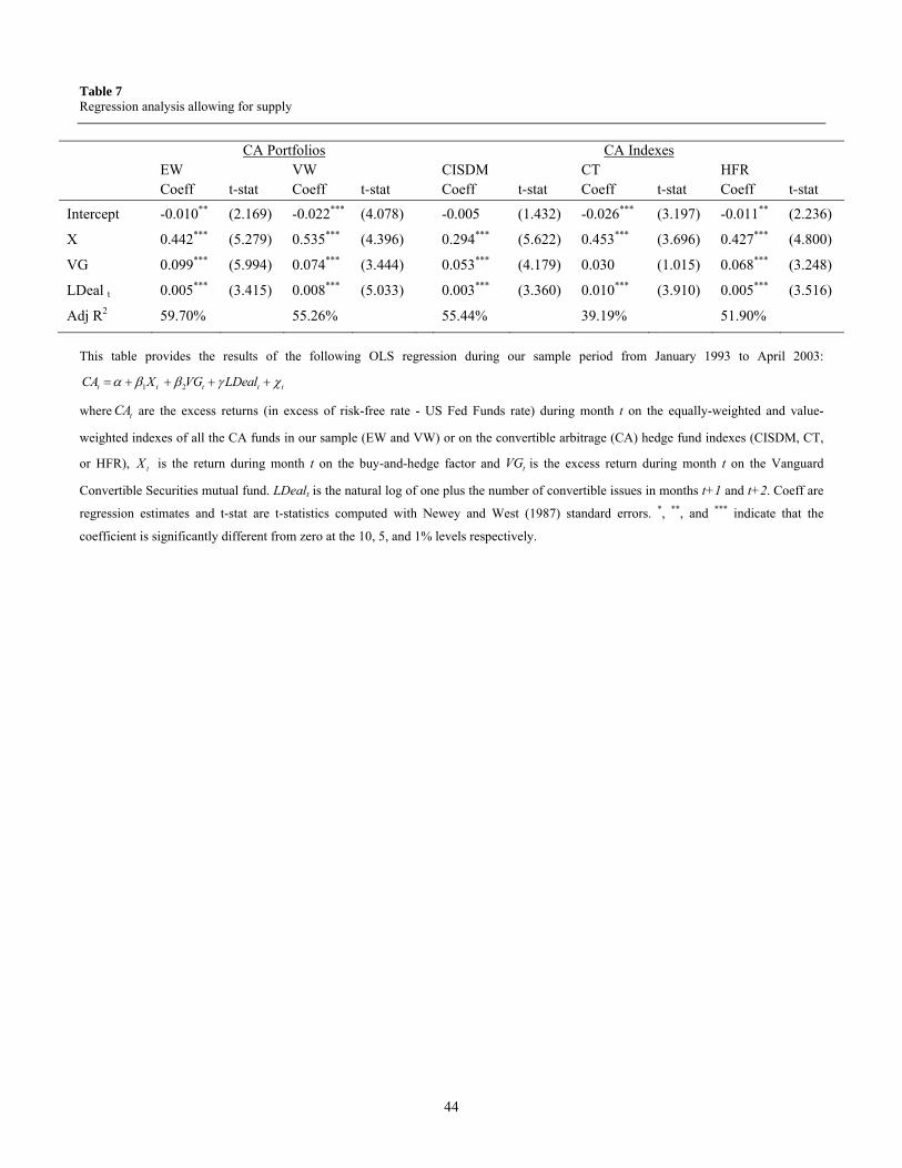
44

Table 7 Regression analysis allowing for supply

CA Portfolios CA Indexes EW VW CISDM CT HFR Coeff t-stat Coeff t-stat Coeff t-stat Coeff t-stat Coeff t-stat

Intercept -0.010** (2.169) -0.022*** (4.078) -0.005 (1.432) -0.026*** (3.197) -0.011** (2.236)

X 0.442*** (5.279) 0.535*** (4.396) 0.294*** (5.622) 0.453*** (3.696) 0.427*** (4.800)

VG 0.099*** (5.994) 0.074*** (3.444) 0.053*** (4.179) 0.030 (1.015) 0.068*** (3.248)

LDeal t 0.005*** (3.415) 0.008*** (5.033) 0.003*** (3.360) 0.010*** (3.910) 0.005*** (3.516)

Adj R2 59.70% 55.26% 55.44% 39.19% 51.90%

This table provides the results of the following OLS regression during our sample period from January 1993 to April 2003:

1 2t t t t tCA X VG LDeal

where tCA are the excess returns (in excess of risk-free rate - US Fed Funds rate) during month t on the equally-weighted and value-

weighted indexes of all the CA funds in our sample (EW and VW) or on the convertible arbitrage (CA) hedge fund indexes (CISDM, CT,

or HFR), tX is the return during month t on the buy-and-hedge factor and tVG is the excess return during month t on the Vanguard

Convertible Securities mutual fund. LDealt is the natural log of one plus the number of convertible issues in months t+1 and t+2. Coeff are

regression estimates and t-stat are t-statistics computed with Newey and West (1987) standard errors. *, **, and *** indicate that the

coefficient is significantly different from zero at the 10, 5, and 1% levels respectively.

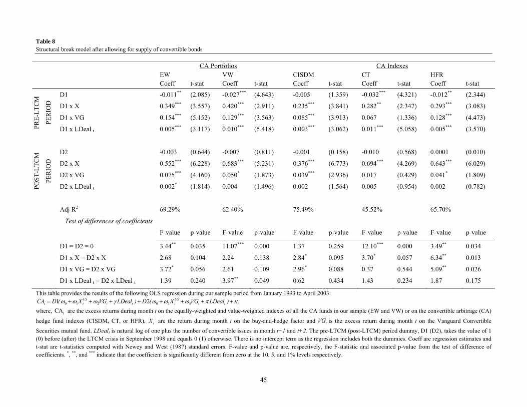
45

Table 8 Structural break model after allowing for supply of convertible bonds

CA Portfolios CA Indexes EW VW CISDM CT HFR Coeff t-stat Coeff t-stat Coeff t-stat Coeff t-stat Coeff t-stat

PR

E-L

TC

M

PE

RIO

D

D1 -0.011** (2.085) -0.027*** (4.643) -0.005 (1.359) -0.032*** (4.321) -0.012** (2.344)

D1 x X 0.349*** (3.557) 0.420*** (2.911) 0.235*** (3.841) 0.282** (2.347) 0.293*** (3.083)

D1 x VG 0.154*** (5.152) 0.129*** (3.563) 0.085*** (3.913) 0.067 (1.336) 0.128*** (4.473)

D1 x LDeal t 0.005*** (3.117) 0.010*** (5.418) 0.003*** (3.062) 0.011*** (5.058) 0.005*** (3.570)

PO

ST

-LT

CM

PE

RIO

D

D2 -0.003 (0.644) -0.007 (0.811) -0.001 (0.158) -0.010 (0.568) 0.0001 (0.010)

D2 x X 0.552*** (6.228) 0.683*** (5.231) 0.376*** (6.773) 0.694*** (4.269) 0.643*** (6.029)

D2 x VG 0.075*** (4.160) 0.050* (1.873) 0.039*** (2.936) 0.017 (0.429) 0.041* (1.809)

D2 x LDeal t 0.002* (1.814) 0.004 (1.496) 0.002 (1.564) 0.005 (0.954) 0.002 (0.782)

Adj R2 69.29% 62.40% 75.49% 45.52% 65.70%

Test of differences of coefficients

F-value p-value F-value p-value F-value p-value F-value p-value F-value p-value

D1 = D2 = 0 3.44** 0.035 11.07*** 0.000 1.37 0.259 12.10*** 0.000 3.49** 0.034

D1 x X = D2 x X 2.68 0.104 2.24 0.138 2.84* 0.095 3.70* 0.057 6.34** 0.013

D1 x VG = D2 x VG 3.72* 0.056 2.61 0.109 2.96* 0.088 0.37 0.544 5.09** 0.026

D1 x LDeal t = D2 x LDeal t 1.39 0.240 3.97** 0.049 0.62 0.434 1.43 0.234 1.87 0.175

This table provides the results of the following OLS regression during our sample period from January 1993 to April 2003:

0 1 2 0 3 41 2US USt t t t t t t tCA D ( X VG LDeal ) D ( X VG LDeal )

where, CAt are the excess returns during month t on the equally-weighted and value-weighted indexes of all the CA funds in our sample (EW and VW) or on the convertible arbitrage (CA)

hedge fund indexes (CISDM, CT, or HFR), tX are the return during month t on the buy-and-hedge factor and tVG is the excess return during month t on the Vanguard Convertible

Securities mutual fund. LDealt is natural log of one plus the number of convertible issues in month t+1 and t+2. The pre-LTCM (post-LTCM) period dummy, D1 (D2), takes the value of 1 (0) before (after) the LTCM crisis in September 1998 and equals 0 (1) otherwise. There is no intercept term as the regression includes both the dummies. Coeff are regression estimates and t-stat are t-statistics computed with Newey and West (1987) standard errors. F-value and p-value are, respectively, the F-statistic and associated p-value from the test of difference of coefficients. *, **, and *** indicate that the coefficient is significantly different from zero at the 10, 5, and 1% levels respectively.

46

Table 9 Individual fund level analyses

Panel A: Two-factor model with supply Size Tercile: Small Medium Large Coeff t-stat Coeff t-stat Coeff t-stat

Intercept -0.002 (-0.552) -0.015*** (-4.281) -0.009*** (-2.863)

X 0.394*** (5.909) 0.419*** (6.624) 0.451*** (7.806)

VG 0.161*** (3.686) 0.127*** (3.185) 0.056 (1.688)

LDeal 0.002 (1.343) 0.006*** (5.914) 0.004*** (4.735)

Adj R2 23.60% 25.41% 18.01%

AUM 8.390 51.088 243.696

# Funds 36 36 36

Mean (%) 0.39 0.65 0.51

Median (%) 0.63 0.78 0.66

SD (%) 1.29 1.05 1.25

47

Panel B: Two-factor model with supply and structural break for the LTCM crisis Size Tercile: Small Medium Large

Coeff t-stat Coeff t-stat Coeff t-stat

PR

E-L

TC

M

PE

RIO

D

D1 -0.013*** (-3.360) -0.018*** (-3.531) -0.028** (-2.589)

D1 x X 0.154* (1.955) 0.407*** (4.547) 0.413** (2.500)

D1 x VG 0.141** (2.678) 0.025 (0.715) 0.079 (1.141)

D1 x LDeal t 0.005*** (5.107) 0.008*** (5.387) 0.010*** (3.080)

PO

ST

-LT

CM

PE

RIO

D

D2 0.017* (1.985) -0.012** (-2.596) -0.009 (-1.638)

D2 x X 0.697 (1.753) 0.677*** (4.347) 0.411*** (3.869)

D2 x VG 0.098*** (3.419) 0.035 (0.953) 0.084 (1.039)

D2 x LDeal t -0.004 (-1.509) 0.005*** (4.018) 0.004 (1.618)

Adj R2 31.84% 43.99% 39.29%

AUM 13.214 63.616 225.036

# Funds 15 15 15

Mean (%) 0.47 0.63 0.48

Median (%) 0.54 0.67 0.77

SD (%) 1.25 0.91 2.12

Test of differences of coefficients Increase Decrease Increase Decrease Increase Decrease

D1 = D2 = 0 3 0 3 0 4 1

D1 x X = D2 x X 3 0 7 1 2 1

D1 x VG = D2 x VG 1 4 2 4 3 1

D1 x LDeal t = D2 x LDeal t 0 2 0 5 1 4

Panel A of this table summarizes the fund level results of the following OLS regression during our sample period from January 1993 to

April 2003: 0 1 2 3t t t t tCA X VG LDeal

where, CAt is the excess return (in excess of risk-free rate, i.e., US Fed Funds rate) during month t on a convertible arbitrage hedge fund

with at least 24 monthly returns during the sample period, tX is the return during month t on the buy-and-hedge factor, tVG is the excess

return during month t on the Vanguard Convertible Securities mutual fund (VG) and LDealt is natural log of one plus the number of

convertible issues in months t+1 and t+2. We sort funds into size terciles based on their average assets under management during the

sample period and summarize the regression outputs of funds in each tercile. Coeff and t-stat are, respectively, the mean and t-statistic of

individual fund regression coefficients. Adj R2 is the average of funds’ adjusted R2. AUM reports the grand average assets under

management (in $ millions) in each tercile and # Funds reports the number of funds in each tercile. Mean, Median, and SD are,

respectively, the mean, median and standard deviation of the monthly excess return on the equally-weighted size tercile. Panel B of this

table provides the results of the following OLS regression during our sample period from January 1993 to April 2003:

0 1 2 0 3 41 2t t t t t t t tCA D ( X VG LDeal ) D ( X VG LDeal )

where, CAt is the excess return (in excess of risk-free rate - US Fed Funds rate) during month t on a convertible arbitrage hedge fund

with at least 48 monthly returns during the sample period and which existed before, during and after the LTCM crisis. The pre-LTCM

(post-LTCM) period dummy, D1 (D2), takes the value of 1 (0) before (after) the LTCM crisis in September 1998 and equals 0 (1)

48

otherwise. There is no intercept term as the regression includes both the dummies. As in Panel A, we summarize the regression outputs of

funds in each tercile. Increase (Decrease) is the number of funds for which there is a statistically significant increase (decrease) in

coefficient after the LTCM crisis. *, **, and *** indicate that the coefficient is significantly different from zero at the 10, 5, and 1% levels

respectively.

49

Table 10 Descriptive Statistics of Convertible Arbitrage Indexes and Factors during the out-of-sample period

Panel A: Summary Statistics Mean (%) Median (%) SD (%) Min. (%) Max. (%) Skew Kurt

VG 0.84 0.95 2.03 -4.25 5.03 -0.17 0.16

CISDM 0.17 0.28 0.83 -2.68 1.98 -0.83 1.77

CT 0.21 0.35 1.03 -3.36 2.39 -0.91 2.08

CTX 0.20 0.24 0.93 -2.59 2.11 -0.37 0.87

HFR 0.13 0.29 0.89 -2.87 2.04 -0.93 1.57

HFRX -0.12 0.14 1.14 -3.68 2.67 -0.78 1.49

Panel B: Correlations between VG, CA indexes and the X factor VG CISDM CT CTX HFR HFRX

VG 1.00

CISDM 0.57*** 1.00

CT 0.60*** 0.95*** 1.00

CTX 0.64*** 0.91*** 0.95*** 1.00

HFR 0.55*** 0.97*** 0.97*** 0.91*** 1.00

HFRX 0.49*** 0.87*** 0.89*** 0.87*** 0.89*** 1.00

OX 0.51*** 0.57*** 0.60*** 0.57*** 0.62*** 0.66***

Panel A of this table provides the descriptive statistics of the monthly returns of the Vanguard Convertible Securities mutual fund (VG),

three convertible arbitrage (CA) indexes (CISDM, CT, HFR) and two convertible arbitrage investable indexes (CTX and HFRX) during

the out-of-sample period (May 2003 to June 2007). VG, CISDM, CT, HFR and HFRX are available for the entire out-of-sample period

while CTX starts in August 2003. The descriptive statistics include mean, median, standard deviation (SD), minimum (Min.), maximum

(Max.), skewness (Skew), and kurtosis (Kurt). Panel B provides correlations between VG, CISDM, CT, CTX, HFR, HFRX and the buy-

and-hedge factor, OX . *, **, and *** indicate that the coefficient is significantly different from zero at the 10, 5, and 1% levels

respectively.

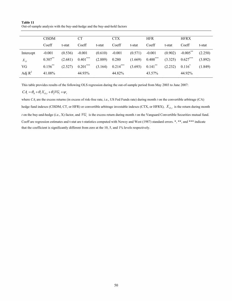
50

Table 11 Out-of-sample analysis with the buy-and-hedge and the buy-and-hold factors

CISDM CT CTX HFR HFRX

Coeff t-stat Coeff t-stat Coeff t-stat Coeff t-stat Coeff t-stat

Intercept -0.001 (0.536) -0.001 (0.610) -0.001 (0.571) -0.001 (0.902) -0.005** (2.250)

OX 0.307** (2.681) 0.401*** (2.889) 0.280 (1.669) 0.400*** (3.325) 0.627*** (3.892)

VG 0.156** (2.527) 0.201*** (3.164) 0.214*** (3.693) 0.141** (2.232) 0.116* (1.849)

Adj R2 41.08% 44.93% 44.82% 43.57% 44.92%

This table provides results of the following OLS regression during the out-of-sample period from May 2003 to June 2007:

0 1 , 2t O t t tCA X VG

where CAt are the excess returns (in excess of risk-free rate, i.e., US Fed Funds rate) during month t on the convertible arbitrage (CA)

hedge fund indexes (CISDM, CT, or HFR) or convertible arbitrage investable indexes (CTX, or HFRX), ,O tX is the return during month

t on the buy-and-hedge (i.e., X) factor, and tVG is the excess return during month t on the Vanguard Convertible Securities mutual fund.

Coeff are regression estimates and t-stat are t-statistics computed with Newey and West (1987) standard errors. *, **, and *** indicate

that the coefficient is significantly different from zero at the 10, 5, and 1% levels respectively.

51

Table 12 Out-of-sample analysis with the buy-and-hedge and the buy-and-hold factors after allowing for supply

CISDM CT CTX HFR HFRX

Coeff t-stat Coeff t-stat Coeff t-stat Coeff t-stat Coeff t-stat

Intercept -0.024** (2.293) -0.034** (2.409) -0.036*** (3.422) -0.027** (2.247) -0.030** (2.047)

OX 0.322*** (3.353) 0.410*** (3.594) 0.257* (1.827) 0.411*** (4.175) 0.641*** (4.265)

VG 0.110* (1.755) 0.139* (1.922) 0.172*** (2.709) 0.088 (1.366) 0.067 (0.869)

LDeal t 0.007** (2.277) 0.009** (2.412) 0.010*** (3.406) 0.007** (2.197) 0.007* (1.783)

Adj R2 48.72% 54.03% 56.44% 50.93% 49.17%

This table provides results of the following OLS regression during the out-of-sample period from May 2003 to June 2007:

1 , 2t O t t t tCA X VG LDeal

where CAt are the excess returns (in excess of risk-free rate, i.e., US Fed Funds rate) during month t on the convertible arbitrage (CA)

hedge fund indexes (CISDM, CT, or HFR) or convertible arbitrage investable indexes (CTX, or HFRX), ,O tX is the return during month t

on the X factor, tVG is the excess return during month t on the Vanguard Convertible Securities mutual fund (VG), LDealt is natural log

of one plus the number of convertible issues in month t+1 and t+2. Coeff are regression estimates and t-stat are t-statistics computed with

Newey and West (1987) standard errors. *, **, and *** indicate that the coefficient is significantly different from zero at the 10, 5, and

1% levels respectively.

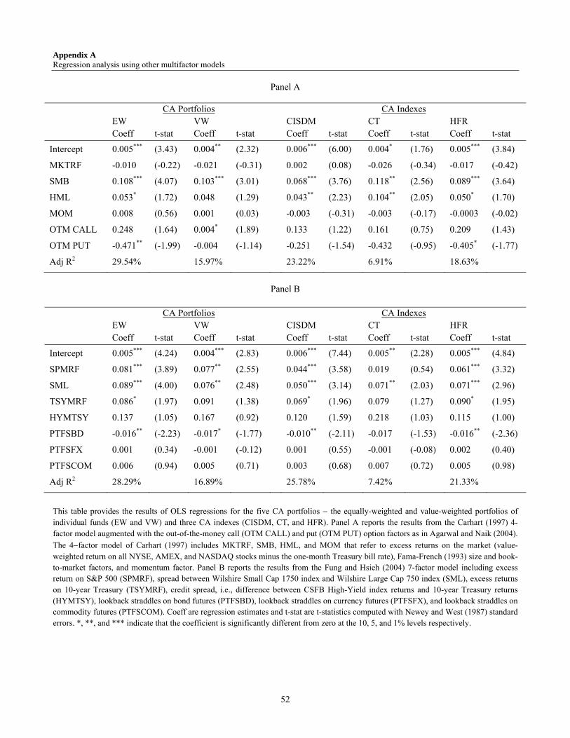
52

Appendix A Regression analysis using other multifactor models

Panel A

CA Portfolios CA Indexes EW VW CISDM CT HFR Coeff t-stat Coeff t-stat Coeff t-stat Coeff t-stat Coeff t-stat

Intercept 0.005*** (3.43) 0.004** (2.32) 0.006*** (6.00) 0.004* (1.76) 0.005*** (3.84)

MKTRF -0.010 (-0.22) -0.021 (-0.31) 0.002 (0.08) -0.026 (-0.34) -0.017 (-0.42)

SMB 0.108*** (4.07) 0.103*** (3.01) 0.068*** (3.76) 0.118** (2.56) 0.089*** (3.64)

HML 0.053* (1.72) 0.048 (1.29) 0.043** (2.23) 0.104** (2.05) 0.050* (1.70)

MOM 0.008 (0.56) 0.001 (0.03) -0.003 (-0.31) -0.003 (-0.17) -0.0003 (-0.02)

OTM CALL 0.248 (1.64) 0.004* (1.89) 0.133 (1.22) 0.161 (0.75) 0.209 (1.43)

OTM PUT -0.471** (-1.99) -0.004 (-1.14) -0.251 (-1.54) -0.432 (-0.95) -0.405* (-1.77)

Adj R2 29.54% 15.97% 23.22% 6.91% 18.63%

Panel B

CA Portfolios CA Indexes EW VW CISDM CT HFR Coeff t-stat Coeff t-stat Coeff t-stat Coeff t-stat Coeff t-stat

Intercept 0.005*** (4.24) 0.004*** (2.83) 0.006*** (7.44) 0.005** (2.28) 0.005*** (4.84)

SPMRF 0.081*** (3.89) 0.077** (2.55) 0.044*** (3.58) 0.019 (0.54) 0.061*** (3.32)

SML 0.089*** (4.00) 0.076** (2.48) 0.050*** (3.14) 0.071** (2.03) 0.071*** (2.96)

TSYMRF 0.086* (1.97) 0.091 (1.38) 0.069* (1.96) 0.079 (1.27) 0.090* (1.95)

HYMTSY 0.137 (1.05) 0.167 (0.92) 0.120 (1.59) 0.218 (1.03) 0.115 (1.00)

PTFSBD -0.016** (-2.23) -0.017* (-1.77) -0.010** (-2.11) -0.017 (-1.53) -0.016** (-2.36)

PTFSFX 0.001 (0.34) -0.001 (-0.12) 0.001 (0.55) -0.001 (-0.08) 0.002 (0.40)

PTFSCOM 0.006 (0.94) 0.005 (0.71) 0.003 (0.68) 0.007 (0.72) 0.005 (0.98)

Adj R2 28.29% 16.89% 25.78% 7.42% 21.33%

This table provides the results of OLS regressions for the five CA portfolios the equally-weighted and value-weighted portfolios of individual funds (EW and VW) and three CA indexes (CISDM, CT, and HFR). Panel A reports the results from the Carhart (1997) 4-factor model augmented with the out-of-the-money call (OTM CALL) and put (OTM PUT) option factors as in Agarwal and Naik (2004).

The 4factor model of Carhart (1997) includes MKTRF, SMB, HML, and MOM that refer to excess returns on the market (value-weighted return on all NYSE, AMEX, and NASDAQ stocks minus the one-month Treasury bill rate), Fama-French (1993) size and book-to-market factors, and momentum factor. Panel B reports the results from the Fung and Hsieh (2004) 7-factor model including excess return on S&P 500 (SPMRF), spread between Wilshire Small Cap 1750 index and Wilshire Large Cap 750 index (SML), excess returns on 10-year Treasury (TSYMRF), credit spread, i.e., difference between CSFB High-Yield index returns and 10-year Treasury returns (HYMTSY), lookback straddles on bond futures (PTFSBD), lookback straddles on currency futures (PTFSFX), and lookback straddles on commodity futures (PTFSCOM). Coeff are regression estimates and t-stat are t-statistics computed with Newey and West (1987) standard errors. *, **, and *** indicate that the coefficient is significantly different from zero at the 10, 5, and 1% levels respectively.

53

Appendix B

In-sample results with the out-of-sample buy-and-hedge factor, XO

CA Portfolios CA Indexes EW VW CISDM CT HFR Coeff t-stat Coeff t-stat Coeff t-stat Coeff t-stat Coeff t-stat

Intercept 0.005*** (4.471) 0.004*** (2.907) 0.006*** (7.467) 0.004** (2.106) 0.005*** (4.634)

OX 0.090* (1.811) 0.151** (2.432) 0.062* (1.780) 0.183** (2.459) 0.104** (1.994)

VG 0.150*** (6.040) 0.142*** (4.463) 0.088*** (4.601) 0.093** (2.301) 0.116*** (4.032)

Adj R2 36.79% 26.64% 31.20% 15.05% 27.82%

This table provides the results of the following OLS regression during our sample period from January 1993 to April 2003:

0 1 2CA VGt Ot t tXh h h p= + + +

where, CAt are the excess returns (in excess of risk-free rate, i.e., US Fed Funds rate) during month t on the equally-weighted

index of all the CA funds in our sample (EW) or on the convertible arbitrage (CA) hedge fund indexes (CISDM, CT, or HFR),

OtX is the return during month t on the out-of-sample X factor constructed using the Russell 2000 index instead of the individual

stock data as described in Section 6.1. tVG is the excess return during month t on the Vanguard Convertible Securities mutual

fund. Coeff are regression estimates and t-stat are t-statistics computed with Newey and West (1987) standard errors. *, **, and ***

indicate that the coefficient is significantly different from zero at the 10, 5, and 1% levels respectively.

54

Fig. 1. Cumulative residuals. This figure presents cumulative residual plots of the equally-weighted size terciles (Small,

Medium, and Large) and the plot of cumulative convertible bond (CB) supply. The plots cover the period surrounding the LTCM

break (March 1998 – July 1999). For each tercile, we first compute monthly residuals for each fund using the fund’s excess

returns, its factor loadings from estimating the structural break model without supply effect, and factor realizations. Once we

have the fund level residuals, we average the residuals across funds each month to obtain the equally-weighted residual for each

tercile. We then cumulate the equally-weighted residuals to obtain cumulative residuals for each tercile.

55

Fig. 2. Cumulative residuals net of supply effect. This figure presents net of supply effect cumulative residual plots of the

equally-weighted size terciles (Small, Medium, and Large) and the plot of cumulative convertible bond (CB) supply. The plots

cover the period surrounding the LTCM break (March 1998 – July 1999). For each tercile, we first compute monthly residuals for

each fund using the fund’s excess returns, its factor loadings from estimating the structural break model with supply effect, factor

realizations, and realizations of supply variable (LDeal). Once we have the fund level residuals, we average the residuals across

funds each month to obtain the equally-weighted residual for each tercile. We then cumulate the equally-weighted residuals to

obtain cumulative residuals for each tercile.

CFR Working Paper Series

Centre for Financial Research Cologne

CFR Working Papers are available for download from www.cfr-cologne.de. Hardcopies can be ordered from: Centre for Financial Research (CFR), Albertus Magnus Platz, 50923 Koeln, Germany. 2011 No. Author(s) Title 11-09 11-08 11-07 11-06 11-05 11-04 11-03 11-02 11-01 2010 No.

V. Agarwal, S. Ray G. Cici, L.-F. Palacios V. Agarwal, G. D. Gay, L. Ling N. Hautsch, D. Hess, D. Veredas G. Cici S. Jank G.Fellner, E.Theissen S.Jank V. Agarwal, C. Meneghetti Author(s)

Determinants and Implications of Fee Changes in the Hedge Fund Industry On the Use of Options by Mutual Funds: Do They Know What They Are Doing? Window Dressing in Mutual Funds The Impact of Macroeconomic News on Quote Adjustments, Noise, and Informational Volatility The Prevalence of the Disposition Effect in Mutual Funds' Trades Mutual Fund Flows, Expected Returns and the Real Economy Short Sale Constraints, Divergence of Opinion and Asset Value: Evidence from the Laboratory Are There Disadvantaged Clienteles in Mutual Funds? The role of Hedge Funds as Primary Lenders Title

10-20 10-19 10-18 10-17 10-16

G. Cici, S. Gibson, J.J. Merrick Jr. J. Hengelbrock, E. Theissen, Ch. Westheide G. Cici, S. Gibson D. Hess, D. Kreutzmann, O. Pucker S. Jank, M. Wedow

Missing the Marks? Dispersion in Corporate Bond Valuations Across Mutual Funds Market Response to Investor Sentiment The Performance of Corporate-Bond Mutual Funds: Evidence Based on Security-Level Holdings Projected Earnings Accuracy and the Profitability of Stock Recommendations Sturm und Drang in Money Market Funds: When Money Market Funds Cease to Be Narrow

10-15 G. Cici, A. Kempf, A. Puetz

Caught in the Act: How Hedge Funds Manipulate their Equity Positions

10-14 J. Grammig, S. Jank Creative Destruction and Asset Prices 10-13 S. Jank, M. Wedow Purchase and Redemption Decisions of Mutual Fund

Investors and the Role of Fund Families 10-12 S. Artmann, P. Finter,

A. Kempf, S. Koch, E. Theissen

The Cross-Section of German Stock Returns: New Data and New Evidence

10-11 M. Chesney, A. Kempf The Value of Tradeability 10-10 S. Frey, P. Herbst The Influence of Buy-side Analysts on

Mutual Fund Trading 10-09 V. Agarwal, W. Jiang,

Y. Tang, B. Yang Uncovering Hedge Fund Skill from the Portfolio Holdings They Hide

10-08 V. Agarwal, V. Fos,

W. Jiang Inferring Reporting Biases in Hedge Fund Databases from Hedge Fund Equity Holdings

10-07 V. Agarwal, G. Bakshi,

J. Huij Do Higher-Moment Equity Risks Explain Hedge Fund Returns?

10-06 J. Grammig, F. J. Peter Tell-Tale Tails 10-05 K. Drachter, A. Kempf Höhe, Struktur und Determinanten der Managervergütung-

Eine Analyse der Fondsbranche in Deutschland 10-04 J. Fang, A. Kempf,

M. Trapp Fund Manager Allocation

10-03 P. Finter, A. Niessen-

Ruenzi, S. Ruenzi The Impact of Investor Sentiment on the German Stock Market

10-02 D. Hunter, E. Kandel,

S. Kandel, R. Wermers Endogenous Benchmarks

10-01 S. Artmann, P. Finter,

A. Kempf Determinants of Expected Stock Returns: Large Sample Evidence from the German Market

2009 No. Author(s) Title 09-17

E. Theissen

Price Discovery in Spot and Futures Markets: A Reconsideration

09-16 M. Trapp Trading the Bond-CDS Basis – The Role of Credit Risk

and Liquidity 09-14 A. Kempf, O. Korn,

M. Uhrig-Homburg The Term Structure of Illiquidity Premia

09-13 W. Bühler, M. Trapp Time-Varying Credit Risk and Liquidity Premia in Bond and

CDS Markets 09-12 W. Bühler, M. Trapp

Explaining the Bond-CDS Basis – The Role of Credit Risk and Liquidity

09-11 S. J. Taylor, P. K. Yadav,

Y. Zhang

Cross-sectional analysis of risk-neutral skewness

09-10 A. Kempf, C. Merkle,

A. Niessen Low Risk and High Return - How Emotions Shape Expectations on the Stock Market

09-09 V. Fotak, V. Raman,

P. K. Yadav Naked Short Selling: The Emperor`s New Clothes?

09-08 F. Bardong, S.M. Bartram,

P.K. Yadav Informed Trading, Information Asymmetry and Pricing of Information Risk: Empirical Evidence from the NYSE

09-07 S. J. Taylor , P. K. Yadav,

Y. Zhang The information content of implied volatilities and model-free volatility expectations: Evidence from options written on individual stocks

09-06 S. Frey, P. Sandas The Impact of Iceberg Orders in Limit Order Books 09-05 H. Beltran-Lopez, P. Giot,

J. Grammig Commonalities in the Order Book

09-04 J. Fang, S. Ruenzi Rapid Trading bei deutschen Aktienfonds: Evidenz aus einer großen deutschen Fondsgesellschaft

09-03 A. Banegas, B. Gillen,

A. Timmermann, R. Wermers

The Performance of European Equity Mutual Funds

09-02 J. Grammig, A. Schrimpf,

M. Schuppli Long-Horizon Consumption Risk and the Cross-Section of Returns: New Tests and International Evidence

09-01 O. Korn, P. Koziol The Term Structure of Currency Hedge Ratios 2008 No. Author(s) Title 08-12

U. Bonenkamp, C. Homburg, A. Kempf

Fundamental Information in Technical Trading Strategies

08-11 O. Korn Risk Management with Default-risky Forwards 08-10 J. Grammig, F.J. Peter International Price Discovery in the Presence

of Market Microstructure Effects 08-09 C. M. Kuhnen, A. Niessen Public Opinion and Executive Compensation 08-08 A. Pütz, S. Ruenzi Overconfidence among Professional Investors: Evidence from

Mutual Fund Managers 08-07 P. Osthoff What matters to SRI investors? 08-06 08-05 08-04

A. Betzer, E. Theissen P. Linge, E. Theissen N. Hautsch, D. Hess, C. Müller

Sooner Or Later: Delays in Trade Reporting by Corporate Insiders Determinanten der Aktionärspräsenz auf Hauptversammlungen deutscher Aktiengesellschaften Price Adjustment to News with Uncertain Precision

08-03 D. Hess, H. Huang,

A. Niessen How Do Commodity Futures Respond to Macroeconomic News?

08-02 R. Chakrabarti,

W. Megginson, P. Yadav Corporate Governance in India

08-01 C. Andres, E. Theissen Setting a Fox to Keep the Geese - Does the Comply-or-Explain

Principle Work? 2007 No. Author(s) Title

07-16

M. Bär, A. Niessen, S. Ruenzi

The Impact of Work Group Diversity on Performance: Large Sample Evidence from the Mutual Fund Industry

07-15 A. Niessen, S. Ruenzi Political Connectedness and Firm Performance:

Evidence From Germany 07-14 O. Korn Hedging Price Risk when Payment Dates are Uncertain 07-13 A. Kempf, P. Osthoff SRI Funds: Nomen est Omen 07-12 J. Grammig, E. Theissen,

O. Wuensche Time and Price Impact of a Trade: A Structural Approach

07-11 V. Agarwal, J. R. Kale On the Relative Performance of Multi-Strategy and Funds of

Hedge Funds 07-10 M. Kasch-Haroutounian,

E. Theissen Competition Between Exchanges: Euronext versus Xetra

07-09 V. Agarwal, N. D. Daniel,

N. Y. Naik Do hedge funds manage their reported returns?

07-08 N. C. Brown, K. D. Wei,

R. Wermers Analyst Recommendations, Mutual Fund Herding, and Overreaction in Stock Prices

07-07 A. Betzer, E. Theissen Insider Trading and Corporate Governance:

The Case of Germany 07-06 V. Agarwal, L. Wang Transaction Costs and Value Premium 07-05 J. Grammig, A. Schrimpf Asset Pricing with a Reference Level of Consumption:

New Evidence from the Cross-Section of Stock Returns 07-04 V. Agarwal, N.M. Boyson,

N.Y. Naik

Hedge Funds for retail investors? An examination of hedged mutual funds

07-03 D. Hess, A. Niessen The Early News Catches the Attention:

On the Relative Price Impact of Similar Economic Indicators 07-02 A. Kempf, S. Ruenzi,

T. Thiele Employment Risk, Compensation Incentives and Managerial Risk Taking - Evidence from the Mutual Fund Industry -

07-01 M. Hagemeister, A. Kempf CAPM und erwartete Renditen: Eine Untersuchung auf Basis

der Erwartung von Marktteilnehmern 2006 No. Author(s) Title 06-13

S. Čeljo-Hörhager, A. Niessen

How do Self-fulfilling Prophecies affect Financial Ratings? - An experimental study

06-12 R. Wermers, Y. Wu,

J. Zechner Portfolio Performance, Discount Dynamics, and the Turnover of Closed-End Fund Managers

06-11 U. v. Lilienfeld-Toal,

S. Ruenzi Why Managers Hold Shares of Their Firm: An Empirical Analysis

06-10 A. Kempf, P. Osthoff The Effect of Socially Responsible Investing on Portfolio Performance

06-09 R. Wermers, T. Yao, J. Zhao

The Investment Value of Mutual Fund Portfolio Disclosure

06-08 M. Hoffmann, B. Kempa The Poole Analysis in the New Open Economy

Macroeconomic Framework

06-07 K. Drachter, A. Kempf, M. Wagner

Decision Processes in German Mutual Fund Companies: Evidence from a Telephone Survey

06-06 J.P. Krahnen, F.A. Schmid, E. Theissen

Investment Performance and Market Share: A Study of the German Mutual Fund Industry

06-05 S. Ber, S. Ruenzi On the Usability of Synthetic Measures of Mutual Fund Net-

Flows 06-04 A. Kempf, D. Mayston Liquidity Commonality Beyond Best Prices

06-03 O. Korn, C. Koziol Bond Portfolio Optimization: A Risk-Return Approach 06-02 O. Scaillet, L. Barras, R.

Wermers False Discoveries in Mutual Fund Performance: Measuring Luck in Estimated Alphas

06-01 A. Niessen, S. Ruenzi Sex Matters: Gender Differences in a Professional Setting 2005

No. Author(s) Title 05-16

E. Theissen

An Analysis of Private Investors´ Stock Market Return Forecasts

05-15 T. Foucault, S. Moinas,

E. Theissen Does Anonymity Matter in Electronic Limit Order Markets

05-14 R. Kosowski,

A. Timmermann, R. Wermers, H. White

Can Mutual Fund „Stars“ Really Pick Stocks? New Evidence from a Bootstrap Analysis

05-13 D. Avramov, R. Wermers Investing in Mutual Funds when Returns are Predictable 05-12 K. Griese, A. Kempf Liquiditätsdynamik am deutschen Aktienmarkt 05-11 S. Ber, A. Kempf,

S. Ruenzi Determinanten der Mittelzuflüsse bei deutschen Aktienfonds

05-10 M. Bär, A. Kempf,

S. Ruenzi Is a Team Different From the Sum of Its Parts? Evidence from Mutual Fund Managers

05-09 M. Hoffmann Saving, Investment and the Net Foreign Asset Position 05-08 S. Ruenzi Mutual Fund Growth in Standard and Specialist Market

Segments 05-07 A. Kempf, S. Ruenzi Status Quo Bias and the Number of Alternatives

- An Empirical Illustration from the Mutual Fund Industry –

05-06 05-05

J. Grammig, E. Theissen H. Beltran, J. Grammig, A.J. Menkveld

Is Best Really Better? Internalization of Orders in an Open Limit Order Book Understanding the Limit Order Book: Conditioning on Trade Informativeness

05-04 M. Hoffmann Compensating Wages under different Exchange rate Regimes 05-03 M. Hoffmann Fixed versus Flexible Exchange Rates: Evidence from

Developing Countries 05-02 A. Kempf, C. Memmel On the Estimation of the Global Minimum Variance Portfolio 05-01 S. Frey, J. Grammig Liquidity supply and adverse selection in a pure limit order

book market

2004 No. Author(s) Title 04-10

N. Hautsch, D. Hess

Bayesian Learning in Financial Markets – Testing for the Relevance of Information Precision in Price Discovery

04-09 A. Kempf,

K. Kreuzberg Portfolio Disclosure, Portfolio Selection and Mutual Fund Performance Evaluation

04-08 N.F. Carline, S.C. Linn,

P.K. Yadav Operating performance changes associated with corporate mergers and the role of corporate governance

04-07 J.J. Merrick, Jr., N.Y.

Naik, P.K. Yadav Strategic Trading Behavior and Price Distortion in a Manipulated Market: Anatomy of a Squeeze

04-06 N.Y. Naik, P.K. Yadav Trading Costs of Public Investors with Obligatory and

Voluntary Market-Making: Evidence from Market Reforms 04-05 A. Kempf, S. Ruenzi Family Matters: Rankings Within Fund Families and

Fund Inflows 04-04 V. Agarwal,

N.D. Daniel, N.Y. Naik Role of Managerial Incentives and Discretion in Hedge Fund Performance

04-03 V. Agarwal, W.H. Fung,

J.C. Loon, N.Y. Naik Risk and Return in Convertible Arbitrage: Evidence from the Convertible Bond Market

04-02 A. Kempf, S. Ruenzi Tournaments in Mutual Fund Families 04-01 I. Chowdhury, M.

Hoffmann, A. Schabert Inflation Dynamics and the Cost Channel of Monetary Transmission

Cfr/University of cologne

Albertus-Magnus-Platz

D-50923 Cologne

Fon +49(0)221-470-6995

Fax +49(0)221-470-3992

Kempf@cfr-Cologne.dewww.cfr-cologne.de