Risk and Capital Management Y - Retail Banking Academy · Risk and Capital Management ......

DO NOT COPY

147© Retail Banking Academy, 2014

RETAIL BANKINGACADEMY

307.Risk and Capital Management

Course Code 307 - Risk and Capital Management

DO NOT COPY

148


Course Code 307 Risk and Capital Management

IntroductionThis module presents an advanced treatment of interest rate risk and liquidity risk management - the two main dimensions of Asset Liability Management (ALM). In addition, credit and counterparty risk management are discussed along with Basel III capital accords. Effective risk governance will also be reviewed. This module concludes with the design and application of stress testing in an Appendix. Accordingly, the focus here may be described as a continuation of module 208 that deals with balance sheet management and related topics such as Macaulay duration and duration gap and capital allocation methods but only for standardised banks. Maturity gap analysis and fundamental principles of liquidity management are presented in module 210 titled, ‘Financial Management’. Finally, module 209 covers capital approaches for IRB banks that include Value at Risk models (e.g., Credit VaR Operational VaR and Market VaR).

Open Question #1

“Do you agree that duration can be misleading when considering interest rate risk for a retail bank over longer time horizons or if yields change substantially?”

In module 208, Basel III is presented within the context of the ‘3 Pillars’ framework. While Pillar 1 sets minimum capital requirements, the optimal level of capital may be higher. However capital is not a substitute for inadequate control or risk management processes. Pillar 2 is based on four core principles. These are:

a) Bank’s own assessment of capital adequacy – have an internal capital adequacy assessment process (ICAAP)b) Supervisory review processc) Capital level that is above the required (regulatory) minimumd) Supervisory intervention

Significantly, interest rate risk in the banking book is dealt with in Pillar 2 and it will be up to national regulators to decide on whether a bank will be required to hold capital against interest rate risk (IRR) in the banking book.*

* See Principles 12 - 15 of the BCBS document ‘Principles for the Management and Supervision of Interest Rate Risk’ (July 2004)


DO NOT COPY



As was observed during the last financial crisis, banks suffered significant losses in their respective trading books that led to at least two major problems: Banks were undercapitalised and incurred severe liquidity problems as undue reliance on wholesale funding proved to be fickle and interbank-funding dried up. As the financial crisis eventually created an economic crisis, there was significant deterioration in bank’s loan assets leading to higher realised credit risk compared to expected levels. This is because banks price loans on the basis of the prevailing yield curve and the perceived riskiness of the borrower. But as was demonstrated in module 102, when the tracking speed and repricing speed differ (as they normally do), banks incur income interest rate risk. This is made worse if yield curve shifts result in unexpected convexity changes since traditional asset liability approaches based on duration gap will be rendered less than effective.

An interesting question arises: are Basel III risks interdependent? For example, is there a relationship between credit risk and liquidity risk? If so, what are the implications for risk management?

The answer to this question is partially answered by Basel (2008) which states, “The fundamental role of banks in the transformation of short-term deposits into long-term loans makes banks inherently vulnerable to liquidity risk.”* But banks naturally incur credit risk in the loan creation process (i.e., banking book) as some obligors default resulting in unexpected losses. For example, if there is an unexpected increase in under-performing loans that arises from an economic downturn, credit risk will increase.

Important Point

The banking book creates credit risk;* duration transformation creates interest rate and liquidity risk.

* Note that credit risk may also be created in the trading book leading to an incremental risk charge (IRC). This is considered later in this chapter

As discussed in Retail Banking I, the financial intermediation and asset transformation process conducted by banks naturally create mismatches in the bank balance sheet. These mismatches give rise to interest rate risk and liquidity risk. Indeed, Asset Liability Management (ALM) is a bank’s strategic focus on the management of its balance sheet in order to manage these two key risks.

The focus of interest rate risk management is typically the market value for shareholder’s equity or net interest income. There is also the consideration of options in balance sheet securities (e.g., callable bonds or residential mortgage-backed securities) where cash flows are affected by changes in yields.

The other focus is on liquidity risk management that arises from a liquidity gap, which is the outcome of differing terms of assets and liabilities on the bank’s balance sheet.

These two dimensions of ALM are considered in Chapter 2.

In previous modules of Retail Banking II, we considered the simple Gap Analysis that is based on the formula that ∆NII = (RSA – RSL) x ∆r. In this equation NII = net interest income, RSA = rate sensitive assets, RSL = rate sensitive liabilities and r = appropriate benchmark rate.†

Among the most important assumptions underlying this analysis is that only parallel shifts in the yield curve are permitted. There are other defects that include neglect of embedded options, but it is typically adopted for its simplicity.However, the Basel Committee Approach‡ is based on this formula. We illustrate it as follows:

* Basel (2009) defines funding liquidity risk as the risk that the firm will not be able to meet efficiently both expected and unexpected current and future cash flow and collateral needs without affecting either daily operations or the financial condition of the firm. This is different from market liquidity risk which Basel (2008) states is the risk that a firm cannot easily offset or eliminate a position at the market price because of inadequate market depth or market disruption† Cumulative gap is considered in Financial Management (210) for the CAMELS model‡ Principles for the Management and Supervision of interest Rate Risk, BCBS: July 2004


DO NOT COPY

150


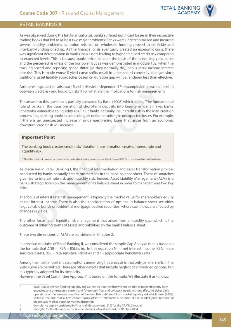
Banks will allocate their assets and liabilities into 14 time bands (see Annex 4 of the BCBS document).

Band Number Time Band Average Maturity (D)

1 Sight 0

2 Up to 1 month 0.5 month

3 From 1 to 3 months 2.0 months

4 From 3 to 6 months 4.5 months

5 From 6 months to 1 year 9 months

6 From 1 year to 2 years 1.5 years

7 From 2 to 3 years 2.5 years



10 From 5 to 7 seven years 6 years




14 Over 20 years 22.5 years

The next step is to convert to average maturity in time band into equivalent modified duration as follows: Divide the average maturity in each time band by a factor that is equal to 1.05. (This is set by BCBS in Annex 4.)

In addition, allocate all the assets and liabilities into each time band and calculate the net position (NP) in each time band.

Finally, for each of the 14 time bands, calculate ΔNPi = −NPi ×MDi ×Δy where ∆y is set at a value of 2 percent.

The bank’s total interest rate risk position is the sum of each risk position for all 14 time bands.

It is noteworthy that the impact on capital for +/- 2 percent interest rate shift should stay within a maximum limit of 20 percent in order to be prudent.

Example:Suppose, for time band 3, the bank allocates assets with a value of $50 million and liabilities equal to $40 million. For this time band, the average maturity of two months converts to modified

duration of 212

×11.05

= 0.1587years . For a net position of $10 million, the change is given

by ∆NP = - $10 million x 0.1587 x 2% = - $31,740.

The total interest rate exposure is the sum of similar calculations for all time bands.


DO NOT COPY



Duration Approach

The duration approach measures the interest rate sensitivity of shareholders’ equity. Specifically, this approach is based on the calculation of the duration gap analysis showing how the market value of shareholder’s equity is expected to change from an anticipated change in interest rates. In particular, as demonstrated in module 208,

DUR Gap= DURA −LA⎛

⎝⎜

⎞

⎠⎟×DURL from which it is derived that DUREquity =

AE×DURGap

In this formula, A = market value of rate sensitive assets and L = market value of rate sensitive liabilities. E = A – L is the market value of shareholders’ equity.

For L less than A, the bank staff would seek to reduce the duration of assets and/or lengthen the duration of liabilities. For example, adjustable rate mortgages may be preferred to reduce asset duration while long-term time deposits may be preferred as a source of funding.

The (Macaulay) duration of equity indicates the expected percentage change in shareholders’ equity from an anticipated change in interest rates. For example, if the benchmark interest rate is expected to increase by 25 basis points from its current value of five percent and the Macaulay duration is 6.5 years, then the market value of shareholders’ equity is expected to decline by apercentage that is equal to DUREquity ×

Δr1+ r

= 6.5× 0.00251.05

= 1.55%

Note that one way to eliminate interest rate risk in shareholders’ equity (i.e., immunisation) is for the bank to formulate appropriate strategies to reduce the value of the duration gap to zero.

Of course the duration gap at zero is equivalent to the statement that DURA

DURL=LA , meaning that

the ratio of the duration of assets to liabilities is equal to the ratio of liabilities to assets. Once abank maintains this relationship, the duration is zero and so shareholder equity is insensitive to interest rate changes (i.e., immunised).

However, the duration gap approach suffers from the fact that it assumes small anticipated changes in interest rates; only parallel shifts in the yield curve are permitted and it neglects embedded options in securities. These defects restrict the application of the duration approach to stabilise interest rate risk in either shareholder equity or net interest income.

For this reason, we present advanced methods for measuring sources of risk in retail banks in Chapter 1. Chapter 2 considers strategies to manage interest rate risk and liquidity risk – the hallmarks of ALM. Chapter 3 comprises an advanced approach to capital allocation for IRB banks and Chapter 4 deals with issues in risk governance. A summary and multiple choice questions follow. Appendix I is a summary of relevant formulae that are applied in this module and Appendix II comprises BCBS stress testing methodology for banks’ balance sheets.


DO NOT COPY

152


Chapter 1:Advanced Concepts in Banking Risk Measurement

Duration and ConvexityWe introduce the concept of convexity to offset for some limitations of duration. this concept is best seen in a graph depicting the relationship between the price of a fixed-income security and its yield to maturity. This is seen below:

Price

Yield

Slope = MD x P (i.e., dollar duration)

Yield

∆ Slope = Convexity x Price

Price

307.1: Relationship between fixed-income security and yield to maturity

The graph shows that the relationship between price and yield is not a straight line. Rather it is convex in that the slope (which is negative) is highest at low levels of the yield to maturity and declines (in absolute value) as yields increase. The slope of this relationship is equal to the modified duration multiplied by the price of the security.

Definition

The slope of the price-yield curve is MD x P where MD is modified duration. This product is called dollar duration.

While duration measures interest rate for individual bonds, the dollar duration measures the total price movement of a specific bond portfolio and hence will be useful for ALM at a strategic level.


DO NOT COPY



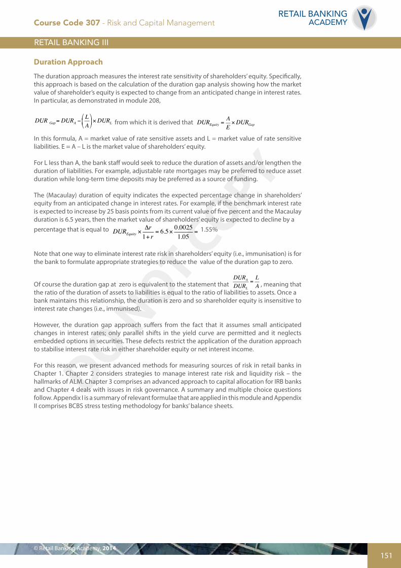
Note that for relatively large changes in interest rates, the slope changes. This means that measuring interest rate risk by duration only, as is the case in traditional duration gap approaches, is more accurate for small changes in interest rates.

For this reason, convexity plays an important role in measuring interest rate risk.

As we see from the graph presented above, the slope becomes less and less negative as yield increases. Convexity is related to the rate of change of the slope of this graph. While the sign of the slope is negative and hence duration is negatively affected, the rate of change of the slope is positive. Hence convexity is positive.

BUT, this is not always the case as will be demonstrated below for securities with embedded options such as mortgage-backed securities.

Convexity is positive for non-callable bonds. A graphical depiction of convexity is shown below:

Price

Yield

Slope = MD x P (i.e., dollar duration)

Yield

∆ Slope = Convexity x Price

Price

307.2: Components of convexity

Definition

Change in Slope is equal to Convexity multiplied by price—i.e., dollar convexity

By observing the shape of the price – yield curve above, it is possible to deduce the following determinants of convexity.

Determinants of Convexity

• For a non-callable bond, convexity is always positive

• All else being equal, there is an inverse relationship between convexity and coupon rate (The higher the coupon rate, the lower is convexity)

• All else being equal, the higher the term of the bond, the higher the convexity

• All else being equal, the higher the yield, the lower the convexity

• Convexity is always less than the square of the maturity of the bond

The combination of duration and convexity more accurately measures interest rate risk in rate- sensitive assets and liabilities on the balance sheet of a bank.

Section A of Appendix 1 considers this issue.


DO NOT COPY

154


Negative Convexity*

Negative convexity arises when the value of certain types of rate sensitive securities falls as interest rates decrease – quite the opposite for their option-free counterparts. For example, as interest rates fall below a certain level, mortgage holders, who typically own a pre-payment option, take advantage of these low rates by paying down their mortgages and refinance at the current lower rates – that is, prepayment speed increases.† But for investors in mortgage-backed securities, they receive payments faster than expected and incur interest rate risk in that they have to reinvest at lower rates.

However, when interest rates increase, mortgage-backed securities behave like regular bonds and their prices. The reason is that the value of the prepayment option is worth less as mortgage owners do not have an incentive to prepay.

Comment

The value of the prepayment is highest when interest rates are low and lowest (even converge to zero) when interest rates are higher.

The value of the prepayment option is inversely proportional to interest rates.

The price-yield relationship for MBS at lower levels of yields is said to reveal ‘negative convexity’. The graph below shows this relationship.

Price

Yield

1.

2.

3.

1. Typical price-yield relationship with Positive Convexity2. Typical price-yield relationship with Negative Convexity 3. Value of Prepayment Option

Payer

Fixed Rate

Floating (LIBOR)

Receiver

Counterparty A

Pays Fixed Rate

Pays LIBOR

Counterparty B

307.3: Negative convexity It is clear that investors in MBS incur a potentially significant interest rate risk arising from negative convexity. Negative convexity limits the rise in price when interest rates are low but accelerates the decline when interest rates rise sufficiently. It is likely for this reason among others that Basel III has higher risk weight for securitised assets such as MBS. Recall from module 208, the general rule is as follows: If a bank retains or acquires a position in a securitisation or has an off-balance

* Negative duration may occur as well. A common example is stripped interest only (IO) MBS. The reason is as follows: If interest rates are expected to rise, the likelihood of prepayment declines. The price of an IO MBS moves in the same direction as interest rate changes, implying a negative duration. An MBS has a positive duration.† Of course, prepayment occurs for other reasons, e.g., homeowners selling their homes.


DO NOT COPY



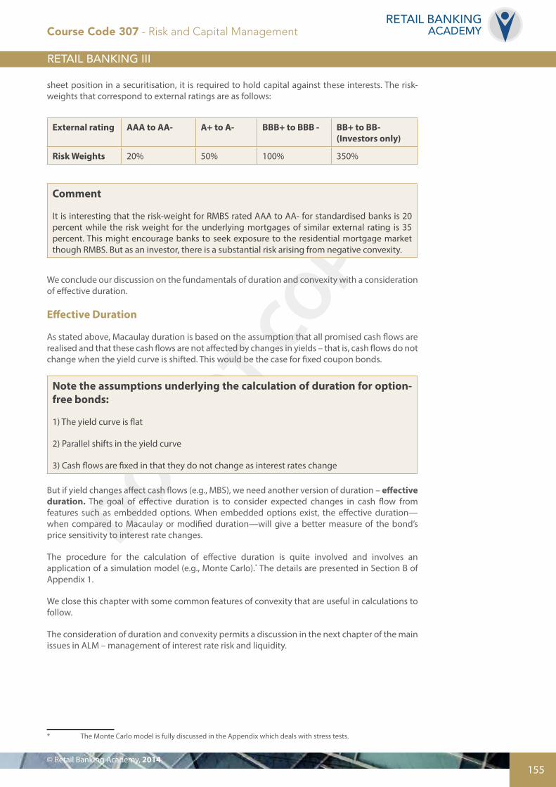
sheet position in a securitisation, it is required to hold capital against these interests. The risk- weights that correspond to external ratings are as follows:

External rating AAA to AA- A+ to A- BBB+ to BBB - BB+ to BB- (Investors only)

Risk Weights 20% 50% 100% 350%

Comment

It is interesting that the risk-weight for RMBS rated AAA to AA- for standardised banks is 20 percent while the risk weight for the underlying mortgages of similar external rating is 35 percent. This might encourage banks to seek exposure to the residential mortgage market though RMBS. But as an investor, there is a substantial risk arising from negative convexity.

We conclude our discussion on the fundamentals of duration and convexity with a consideration of effective duration.

Effective Duration

As stated above, Macaulay duration is based on the assumption that all promised cash flows are realised and that these cash flows are not affected by changes in yields – that is, cash flows do not change when the yield curve is shifted. This would be the case for fixed coupon bonds.

Note the assumptions underlying the calculation of duration for option-free bonds:

1) The yield curve is flat

2) Parallel shifts in the yield curve

3) Cash flows are fixed in that they do not change as interest rates change

But if yield changes affect cash flows (e.g., MBS), we need another version of duration – effective duration. The goal of effective duration is to consider expected changes in cash flow from features such as embedded options. When embedded options exist, the effective duration —when compared to Macaulay or modified duration—will give a better measure of the bond’s price sensitivity to interest rate changes.

The procedure for the calculation of effective duration is quite involved and involves an application of a simulation model (e.g., Monte Carlo).* The details are presented in Section B of Appendix 1.

We close this chapter with some common features of convexity that are useful in calculations to follow.

The consideration of duration and convexity permits a discussion in the next chapter of the main issues in ALM – management of interest rate risk and liquidity.

* The Monte Carlo model is fully discussed in the Appendix which deals with stress tests.


DO NOT COPY

156


Chapter 2: Asset liability Management – Interest Rate Risk and Liquidity Management

Part A: Managing Interest Rate Risk

As stated and demonstrated in module 208, one way to eliminate interest rate risk in shareholders’ equity (i.e., immunisation) is for the bank to formulate appropriate strategies to reduce the value of the duration gap to zero. But this strategy may be misleading since convexity is neglected. Section C of Appendix 1 considers both the duration gap and convexity gap formulae.

Example

Suppose a bank has a single asset that is a perpetuity paying $80,000 annually and yielding 8 percent. This means the current value is $80,000 / 0.08 = $1,000.000. There is also a single liability which is a perpetuity that pays $45,000 annually and which yields 6 percent. The current value is $45,000 / 0.06 = $750 million. The resulting value of shareholders’ equity is $250 million. The modified duration of a perpetuity is 1 / yield so that it is 12.5 for the asset and 16.67 for the liability.

Hence the duration gap is 12.5 - (750/1000) * 16.67 = 0.

This is only part of the analysis – what about the convexity gap?

The convexity for the asset = 2 *(12.5)2 = 312.5 and for the liability is 555.55. This gives a convexity gap of (312.5 – 0.75 * 555.55) =-104.16.

The conclusion is that while the duration gap is zero, the convexity gap is negative. This means that a change in yield (in either direction) will lead to a reduction in shareholders’ equity.

Lesson

Immunisation of shareholders’ equity that seeks to reduce the duration gap to zero must also ensure that the convexity gap is positive.

For a more general approach where the assumption that the average rate of the asset yield is equal to the average liability yield is relaxed, see section D of Appendix I.


DO NOT COPY



Comment

• If bank assets are more sensitive (compared to bank liabilities) to the benchmark rate there are two choices available. The bank may reduce the duration of assets by replacing high duration assets (e.g., long-term fixed rate loans with adjustable rate loans). Algebraically, the right hand side of the above equation will rise and so steps must be taken to reduce the left hand side.

• Alternatively, the bank may increase the duration of liabilities by replacing short-term deposits with long-term fixed-rate time deposits.

• The opposite conclusions may be obtained if bank assets are less sensitive to market interest rate changes when compared to bank liabilities.

But the recommendations for asset or liability restructuring may involve expensive transactions costs and may not be feasible. This is where interest rate derivatives can play an important role in modifying asset and liability durations without outright sale of portfolio securities.

The Role of Interest Rate Derivatives in Interest Rate Risk ManagementIn this section we consider the application of interest rate swaps in managing duration gaps.

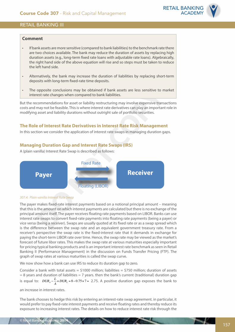
Managing Duration Gap and Interest Rate Swaps (IRS)A (plain vanilla) Interest Rate Swap is described as follows:

Price

Yield

1.

2.

3.


Payer

Fixed Rate

Floating (LIBOR)

Receiver

Counterparty A

Pays Fixed Rate

Pays LIBOR

Counterparty B

307.4: Plain vanilla Interest Rate Swap

The payer makes fixed-rate interest payments based on a notional principal amount – meaning that this is the amount on which interest payments are calculated but there is no exchange of the principal amount itself. The payer receives floating rate payments based on LIBOR. Banks can use interest rate swaps to convert fixed-rate payments into floating rate payments (being a payer) or vice versa (being a receiver). Swaps are usually quoted at its fixed rate or as a swap spread which is the difference between the swap rate and an equivalent government treasury rate. From a receiver’s perspective the swap rate is the fixed-interest rate that it demands in exchange for paying the short-term LIBOR rate over time. Hence, the swap rate may be viewed as the market’s forecast of future libor rates. This makes the swap rate at various maturities especially important for pricing typical banking products and is an important interest rate benchmark as seen in Retail Banking II (Performance Management) in the discussion on Funds Transfer Pricing (FTP). The graph of swap rates at various maturities is called the swap curve.

We now show how a bank can use IRS to reduce its duration gap to zero.

Consider a bank with total assets = $1000 million; liabilities = $750 million; duration of assets = 8 years and duration of liabilities = 7 years. then the bank’s current (traditional) duration gap

is equal to: DURA −LA×DURL = 8− 0.75× 7 = 2.75. A positive duration gap exposes the bank to

an increase in interest rates.

The bank chooses to hedge this risk by entering an interest-rate swap agreement. in particular, it would prefer to pay fixed-rate interest payments and receive floating rates and thereby reduce its exposure to increasing interest rates. The details on how to reduce interest rate risk through the


DO NOT COPY

158


use of interest rate swaps is presented in section E of Appendix 1.

Part B: Managing Liquidity Risk

Module 208 on Balance Sheet Management has provided an extensive description of liquidity risk that arises from the typical financial intermediation process of banks. We also presented a detailed description of the new Basel III liquidity standards (LCR and NSFR) as well as recent developments with respect to level 2 assets in lCR. We repeat for emphasis and for continuity. Recall that LCR is the bank’s first line of defence against liquidity shocks while NSFR is intended to promote prudent funding structures by banks and reduce the propensity to over-rely on short-term wholesale funding.

Liquidity Coverage Ratio

(BCBS Consultative Document, 16 April 2010)

Objective

This metric aims to ensure that a bank maintains an adequate level of unencumbered, high- quality assets that can be converted into cash to meet its liquidity needs for a 30-day time horizon under an acute liquidity-stress scenario specified by supervisors. At a minimum, the stock of liquid assets should enable the bank to survive until Day 30 of the proposed stress scenario, by which time it is assumed that appropriate actions can be taken by management and/or supervisors, and/or the bank can be resolved in an orderly way.

Eligible assets include two levels:

• Level 1 assets comprising cash, central bank reserves and high-quality government debt.

• Level 2 assets include high-quality (AA- and better) corporate and covered bonds. Level 2 assets are subject to 15 per cent haircuts and limited to 40 percent of LCR liquid assets.

Asset-backed securities (ABS) are excluded from LCR, making them less attractive for banks – especially versus covered bonds. LCR = (Stock of high-quality liquid assets) divided by (net cash outflows over a 30-day time period) ≥ 100 percent.

The denominator of the LCR is calculated as follows:

Total Net Cash Outflows (over the next 30 calendar days) = Outflows – Min [Inflows; 75 percent of outflows]

LCR Update

Level 2 assets are divided into two classes - level 2A and level 2B. Furthermore, the original level 2 class (see box above) are now called level 2A. The new class (level 2B) include certain residential mortgage–backed securities (RMBS) rated AA or higher but subject to 25 percent haircut; corporate bonds that do not* meet level 2A requirements but which have external ratings from A+ to and including BBB, which are subject to 50 percent haircut and certain equities which are subject to 50 percent haircut. These level 2B assets can be more than 15 percent of the total high-quality liquid assets (HQLA); they must also be part of the 40 percent cap on total level 2 assets.

Finally, there have been changes in the calculation of net cash flows (in the denominator of theLCR ratio). For example, fully insured (i.e., stable) deposits now have a run-off rate of three percent

* For example, the underlying mortgages must be full recourse – in the event of foreclosure, the borrower is fully liable for any shortfall between the value of the mortgage and the amount obtained upon the sale of the property


DO NOT COPY



instead of the previous five percent.

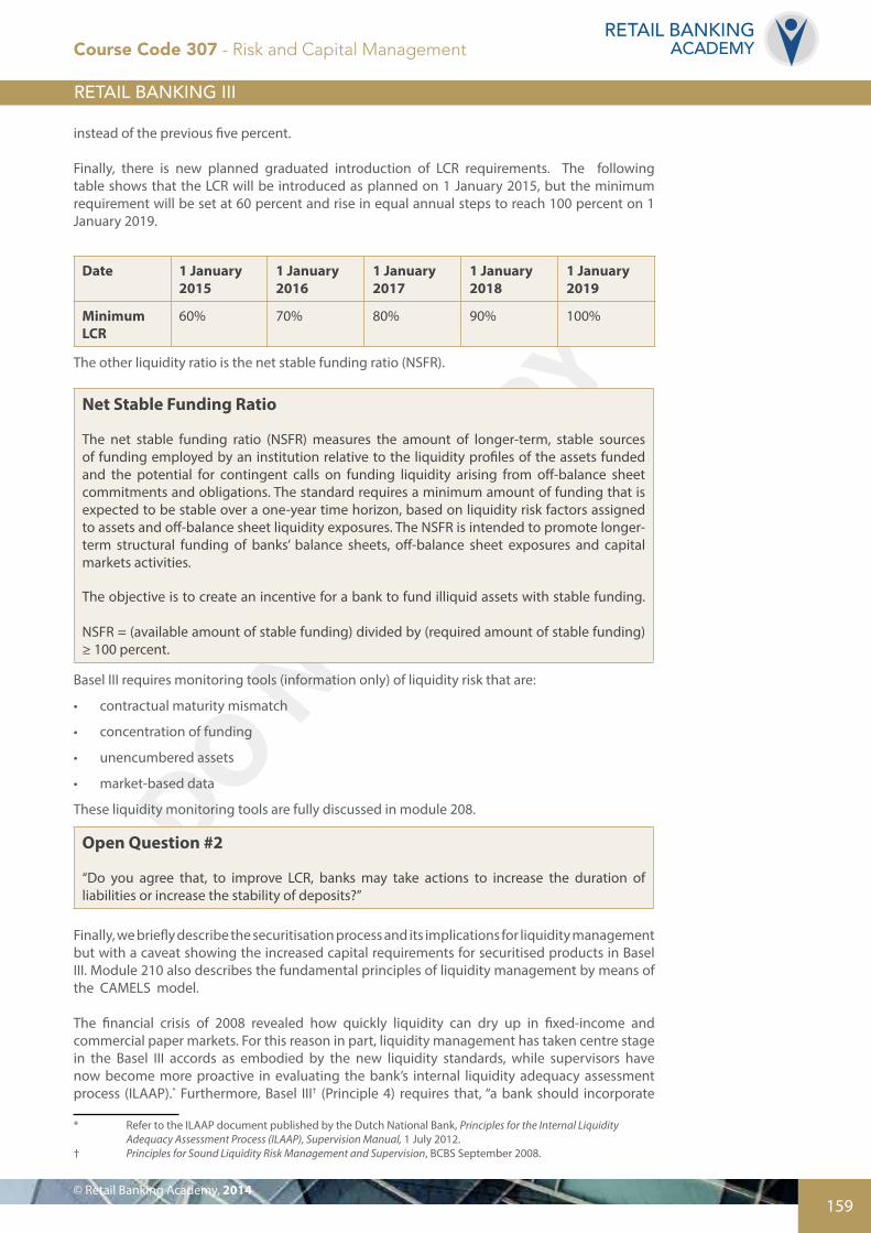
Finally, there is new planned graduated introduction of LCR requirements. The following table shows that the LCR will be introduced as planned on 1 January 2015, but the minimum requirement will be set at 60 percent and rise in equal annual steps to reach 100 percent on 1 January 2019.

Date 1 January2015

1 January2016

1 January2017

1 January2018

1 January2019

Minimum LCR

60% 70% 80% 90% 100%

The other liquidity ratio is the net stable funding ratio (NSFR).

Net Stable Funding Ratio

The net stable funding ratio (NSFR) measures the amount of longer-term, stable sources of funding employed by an institution relative to the liquidity profiles of the assets funded and the potential for contingent calls on funding liquidity arising from off-balance sheet commitments and obligations. The standard requires a minimum amount of funding that is expected to be stable over a one-year time horizon, based on liquidity risk factors assigned to assets and off-balance sheet liquidity exposures. The NSFR is intended to promote longer- term structural funding of banks’ balance sheets, off-balance sheet exposures and capital markets activities.

The objective is to create an incentive for a bank to fund illiquid assets with stable funding. NSFR = (available amount of stable funding) divided by (required amount of stable funding) ≥ 100 percent.

Basel III requires monitoring tools (information only) of liquidity risk that are:

• contractual maturity mismatch

• concentration of funding

• unencumbered assets

• market-based data

These liquidity monitoring tools are fully discussed in module 208.

Open Question #2

“Do you agree that, to improve LCR, banks may take actions to increase the duration of liabilities or increase the stability of deposits?”

Finally, we briefly describe the securitisation process and its implications for liquidity management but with a caveat showing the increased capital requirements for securitised products in Basel III. Module 210 also describes the fundamental principles of liquidity management by means of the CAMELS model.

The financial crisis of 2008 revealed how quickly liquidity can dry up in fixed-income and commercial paper markets. For this reason in part, liquidity management has taken centre stage in the Basel III accords as embodied by the new liquidity standards, while supervisors have now become more proactive in evaluating the bank’s internal liquidity adequacy assessment process (ILAAP).* Furthermore, Basel III† (Principle 4) requires that, “a bank should incorporate

* Refer to the ILAAP document published by the Dutch National Bank, Principles for the Internal Liquidity Adequacy Assessment Process (ILAAP), Supervision Manual, 1 July 2012.† Principles for Sound Liquidity Risk Management and Supervision, BCBS September 2008.


DO NOT COPY

160


liquidity costs, benefits and risks in the product pricing, performance measurement and new product approval process for all significant business activities (both on- and off-balance sheet), thereby aligning the risk-taking incentives of individual business lines with the liquidity risk exposures their activities create for the bank as a whole.” Similar statements are made by FSA in the document ‘Strengthening Liquidity Standards’ (October 2009) and EBA (March 2010) in ‘Guidelines in Liquidity Cost Benefit Allocation’. The FSA document recognises the benefits of Liquidity Transfer Pricing (LTP) for product pricing, performance management and incentives and new product approval.

So how does funding liquidity risk arise in typical banking operations?

An answer is provided in previous modules cited above and also by BCBS (September 2008) where it is stated that maturity transformation “makes banks inherently vulnerable to liquidity risk.” We provide a succinct perspective by quoting from an article by Moorad Chaudhry – member of the advisory board of OMFIF – which was published in the OMFIF Bulletin, January 2013.

Maturity transformation is the essence of banking. This naturally involves a degree of risk. So how does one mitigate it?

The basis of banking is to ‘borrow short to lend long’. By definition, banks never raise liabilities of similar contractual tenor to assets. That’s the nature of supply and demand for cash. The very act of banking demands that we assume something that can never be guaranteed: the ability continuously to roll over required funding. Banks do not fund on a matched basis, because such practice is a practical impossibility. (It is debatable whether they would do so even if they could).

So it’s necessary to address the liquidity gap risk by other means. When allowing for the ‘behaviouralised’ tenor of assets and liabilities, a substantial funding gap remains. Basel III seeks to address this issue with its LCR and NSFR liquidity regime, discussed in Part 1 of this series (OMFIF Monthly Bulletin, January 2013, p16).

Yet bankers commonly say that ‘liquidity risk management’ is more than just these two ratios, and conversely that these two ratios do not capture all the nuances of liquidity risk.

The most effective response to funding risk is a back-to-basics regime. This means changes to prevailing bank business models. The current ones were developed to address the globalised era and the need to reduce costs to remain competitive. Paradoxically, the threat to Western economies comes from Asia-Pacific countries, yet the banks in that region exhibit a more conservative liquidity regime than those in the west.

Rather than focus solely on the two metrics, a more natural approach to liquidity risk would be to accept that the business model has changed, principally due to the need to incorporate the three key mitigants of funding risk: a material share of contractual term funding, a genuinely liquid ‘liquidity portfolio’, and a robust internal funding regime. (Markets call that ‘funds transfer pricing’ but it is more accurately termed an internal borrowing or lending rate).

The first requirement is self-evident. Since continuous liquidity cannot be assured under all circumstances, it is necessary to have a sufficient share of balance sheet funding comprised of long-dated liabilities.

The second requirement arises from the same reality. Liquidity needs to be maintained in cash or liquid assets.


DO NOT COPY



The third requirement is as important as the first two but frequently misrepresented. To ensure that assets generating liquidity stress on the balance sheet are adequately priced, it is necessary to incorporate the correct term liquidity premium at the origination level.

Unfortunately this is often confused with the need to pass on the bank’s marginal funding cost in the internal pricing methodology, rather than the price of pure term liquidity, and so has the potential to become contentious. In fact, a robust approach to internal funds pricing is the key control mechanism reducing the chances of another liquidity crash occurring in the near future.

Taking from the Moorad Choudhry’s article and also from the discussion of funds transfer pricing in the ‘Performance Management’ module, we now present an analysis of liquidity transfer pricing.

The objective of liquidity transfer pricing (LTP) is to reward business units for the liquidity value of deposits, charge assets for inherent liquidity risks and thereby inform marketing for proper product pricing.

Objective of LTP: Reward liquidity Providers and Charge Liquidity Users.

The liquidity-related components of the Liquidity Transfer Pricing (LTP) are as follows:

Funding Liquidity Spread, which is the expected cost of funds to support the bank exposure to its remaining maturity. Contingent Liquidity Spread is the expected cost of funds to maintain a sufficient buffer of high quality liquid assets (HQLA) to meet unexpected obligation. The Liquidity adjusted FTP = Reference Swap Rate + Credit Spread + Option Spread + Contingent Liquidity Spread + Funding Liquidity Spread.


DO NOT COPY

162


Chapter 3: Capital Allocation for Internal Ratings Based (IRB) Banks

Capital allocation for standarised banks is fully discussed in Retail Banking II. Let us now consider IRB banks for each of the Basel risks in turn.

Credit Risk*

Some of the following discussion is based on the BCBS document cited in footnote 12.

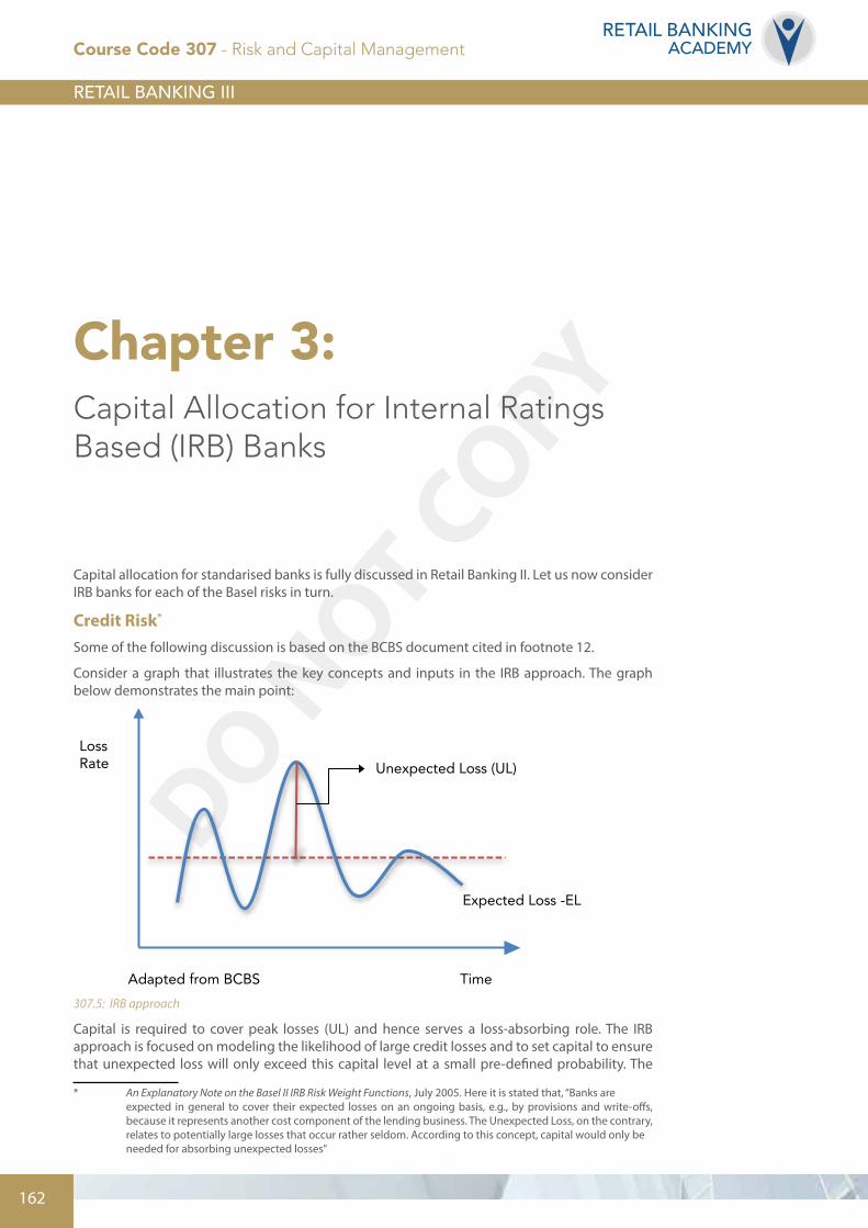
Consider a graph that illustrates the key concepts and inputs in the IRB approach. The graph below demonstrates the main point:

LossRate

Time

Unexpected Loss (UL)

Expected Loss -EL

Adapted from BCBS

Frequency

Loss

100% - confidence level

EL (Provisions) UL (Capital)

Value at Risk (VaR)

307.5: IRB approach

Capital is required to cover peak losses (UL) and hence serves a loss-absorbing role. The IRB approach is focused on modeling the likelihood of large credit losses and to set capital to ensure that unexpected loss will only exceed this capital level at a small pre-defined probability. The

* An Explanatory Note on the Basel II IRB Risk Weight Functions, July 2005. Here it is stated that, “Banks are expected in general to cover their expected losses on an ongoing basis, e.g., by provisions and write-offs, because it represents another cost component of the lending business. The Unexpected Loss, on the contrary, relates to potentially large losses that occur rather seldom. According to this concept, capital would only be needed for absorbing unexpected losses”


DO NOT COPY



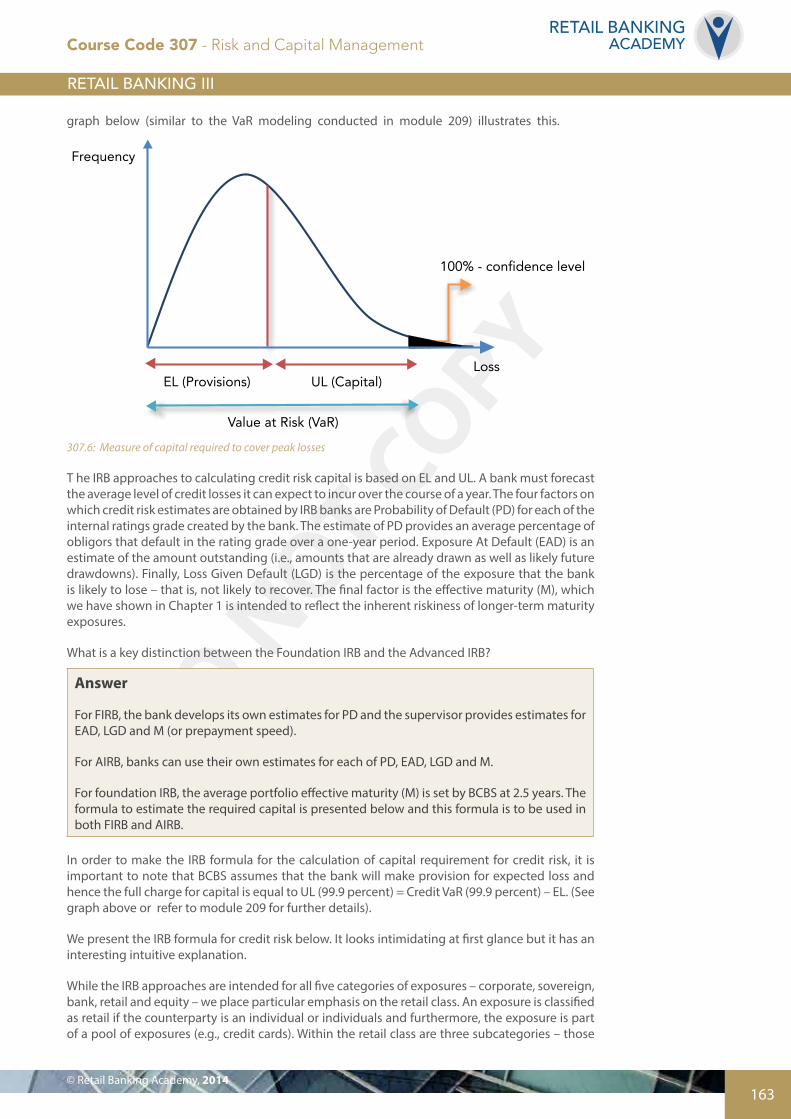
graph below (similar to the VaR modeling conducted in module 209) illustrates this.

LossRate

Time

Unexpected Loss (UL)

Expected Loss -EL

Adapted from BCBS

Frequency

Loss

100% - confidence level

EL (Provisions) UL (Capital)

Value at Risk (VaR)

307.6: Measure of capital required to cover peak losses

T he IRB approaches to calculating credit risk capital is based on EL and UL. A bank must forecast the average level of credit losses it can expect to incur over the course of a year. The four factors on which credit risk estimates are obtained by IRB banks are Probability of Default (PD) for each of the internal ratings grade created by the bank. The estimate of PD provides an average percentage of obligors that default in the rating grade over a one-year period. Exposure At Default (EAD) is an estimate of the amount outstanding (i.e., amounts that are already drawn as well as likely future drawdowns). Finally, Loss Given Default (LGD) is the percentage of the exposure that the bank is likely to lose – that is, not likely to recover. The final factor is the effective maturity (M), which we have shown in Chapter 1 is intended to reflect the inherent riskiness of longer-term maturity exposures.

What is a key distinction between the Foundation IRB and the Advanced IRB?

Answer

For FIRB, the bank develops its own estimates for PD and the supervisor provides estimates for EAD, LGD and M (or prepayment speed).

For AIRB, banks can use their own estimates for each of PD, EAD, LGD and M.

For foundation IRB, the average portfolio effective maturity (M) is set by BCBS at 2.5 years. The formula to estimate the required capital is presented below and this formula is to be used in both FIRB and AIRB.

In order to make the IRB formula for the calculation of capital requirement for credit risk, it is important to note that BCBS assumes that the bank will make provision for expected loss and hence the full charge for capital is equal to UL (99.9 percent) = Credit VaR (99.9 percent) – EL. (See graph above or refer to module 209 for further details).

We present the IRB formula for credit risk below. It looks intimidating at first glance but it has an interesting intuitive explanation.

While the IRB approaches are intended for all five categories of exposures – corporate, sovereign, bank, retail and equity – we place particular emphasis on the retail class. An exposure is classified as retail if the counterparty is an individual or individuals and furthermore, the exposure is part of a pool of exposures (e.g., credit cards). Within the retail class are three subcategories – those


DO NOT COPY

164


secured by residential properties, qualifying revolving retail exposures and other retail exposures.

The IRB Approach for Retail Credit Exposures

Notwithstanding the distinction between FIRB and AIRB, retail banks have to calculate their own estimates of PD, LGD and EAD. In addition, there is no maturity adjustment in the risk weight function for capital calculation.

The formula (presented in the footnote below)* to calculate the risk weight for retail exposures, not in default, is based on the following inputs:

• The minimum period of historical data in order to estimate PD and LGD is five years. Banks provide estimates of PD and LGD based on the appropriate pool. This pool is assigned to an internal rating grade and PD has a minimum value of 0.03 percent. For retail exposures based on secured residential properties, the minimum LGD is 20 percent for input in the formula in the footnote below†. Adjustments for guarantees and credit derivatives that are risk-reducing are accounted for in either PD or LGD estimates.

• Similar to PD and LGD, a minimum of five years of data is required to estimate EAD. Adjustment to EAD or LGD (which is inversely related to recovery rate) is required to account for uncertain future drawdowns prior to default.

• The correlation (R) of the retail exposure with the global economy – a systemic relationship.

• For each of the three categories of retail exposures, BCBS specifies fixed values for R. These are as follows: R = 15 percent for residential mortgage exposures R = 4 percent for qualifying revolving retail exposures R is between 3 percent and 16 percent for other retail exposures† (See footnote below† for the formula for R in this case)

The estimate for the risk weight (K) from the formula in the footnote below* provides a value of risk- weighted assets given by: RWA = K x 12.5 x EAD where the factor 12.5 is the inverse of 8%.

Of course the capital charge = K x EAD.

We present an example to illustrate the full procedure for a pool of residential mortgage exposures.

Example

A retail bank has obtained the following estimates, based on five-year historical data. The probability of default (PD) = 0.03 percent; Loss given default (LGD) = 20 percent; Exposure at Default (EAD) = $1 million. The correlation coefficient (R) is set at 15 percent (BCBS). Using the formula presented in Section F of Appendix 1, we obtain a value of 1.74 percent for K.

Then the appropriate capital charge is 1.74 percent of EAD = 1.74 percent x $1million =$17,400. The value of RWA = K x 12.5 x $1million = $217,500.

Let us now consider the capital charge for counterparty credit risk.

* K = LGD×N G(PD)(1− R)0.5

+R0.5

(1− R)0.5×G(0.999)

⎛

⎝⎜

⎞

⎠⎟− LGD*PD where N is the cumulative normal distribution; G is the

inverse of the cumulative normal distribution; R is the correlation coefficient of the retail exposure with the market; LGD and PD are calculated as percentages of EAD”

† R = 0.03× 1− exp(−35×PD)1− exp(−35)

⎛

⎝⎜

⎞

⎠⎟+ 0.16× 1−

1− exp(−35×PD1− exp(−35×PD)

⎛

⎝⎜

⎞

⎠⎟


DO NOT COPY



Counterparty Credit Risk (CCR)

The financial crisis has shown that derivatives-trading has the potential for counterparty failures (e.g., Lehman, AIG, etc). The resulting contagion effects and serious global economic downturn are well known. While there are many alleged reasons for the 2008 financial crisis, undoubtedly counterparty failure in over-the-counter (OTC) derivative transactions played a key role. While these counterparty failures were largely within the domain of wholesale and investment banking, counterparty risk is still important for retail banks. For example, we have shown above how retail banks in managing interest rate risk, can alter their duration gap with the use of interest rate swaps.

Counterparty Credit Risk (CRR) is the risk that a counterparty in a financial contract may default on its obligations during the term of the contract. It is important to note that CRR is different from credit risk created by a bank though the lending process. In this case, the exposure is one-sided in the sense that only the lending bank faces the risk of a loss – sometimes called ‘issuer risk’. Counterparty credit risk is bilateral in the sense that each counterparty has an exposure to the other counterparty. This is because the market value of the transaction varies over time and can be negative or positive from the perspective of either counterparty.

The concept is labeled ‘Credit Valuation Adjustment’ (CVA), and calculates the net credit exposure faced by one counterparty in the transaction. It is a valuation adjustment to the typical approaches in the literature (especially pre-2008) which modeled derivatives on the basis of zero counterparty credit risk.

CVA covers the risk to either counterparty for possible deterioration of credit quality of other counterparties over the time period of the transaction.

There is a presumption that OTC-derivative transactions that are subject to bilateral clearing are more prone to counterparty risk. Indeed, in a press release of 1 June 2011, the BCBS stated that about two-thirds of losses attributed to counterparty credit risks were due to CVA losses, and only about one-third were due to actual defaults.

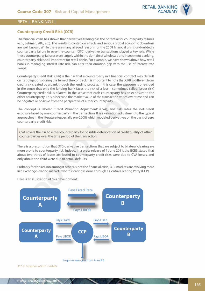
Probably for this reason amongst others, since the financial crisis, OTC markets are evolving more like exchange–traded markets where clearing is done through a Central Clearing Party (CCP).

Here is an illustration of this development:

Price

Yield

1.

2.

3.


Payer

Fixed Rate

Floating (LIBOR)

Receiver

Counterparty A

Pays Fixed Rate

Pays LIBOR

Counterparty B

Counterparty A

Pays Fixed

Pays LIBOR

Counterparty BCCP

Pays Fixed

Pays LIBOR

Requires margins from A and B

Frequency Probability

+# Loss Events Severity of Loss

=Probability

OP VaR (α)

α = 0.1%

Required Capital (K) = OP VaR assuming that EL is not provisioned.

307.7: Evolution of OTC markets


DO NOT COPY

166


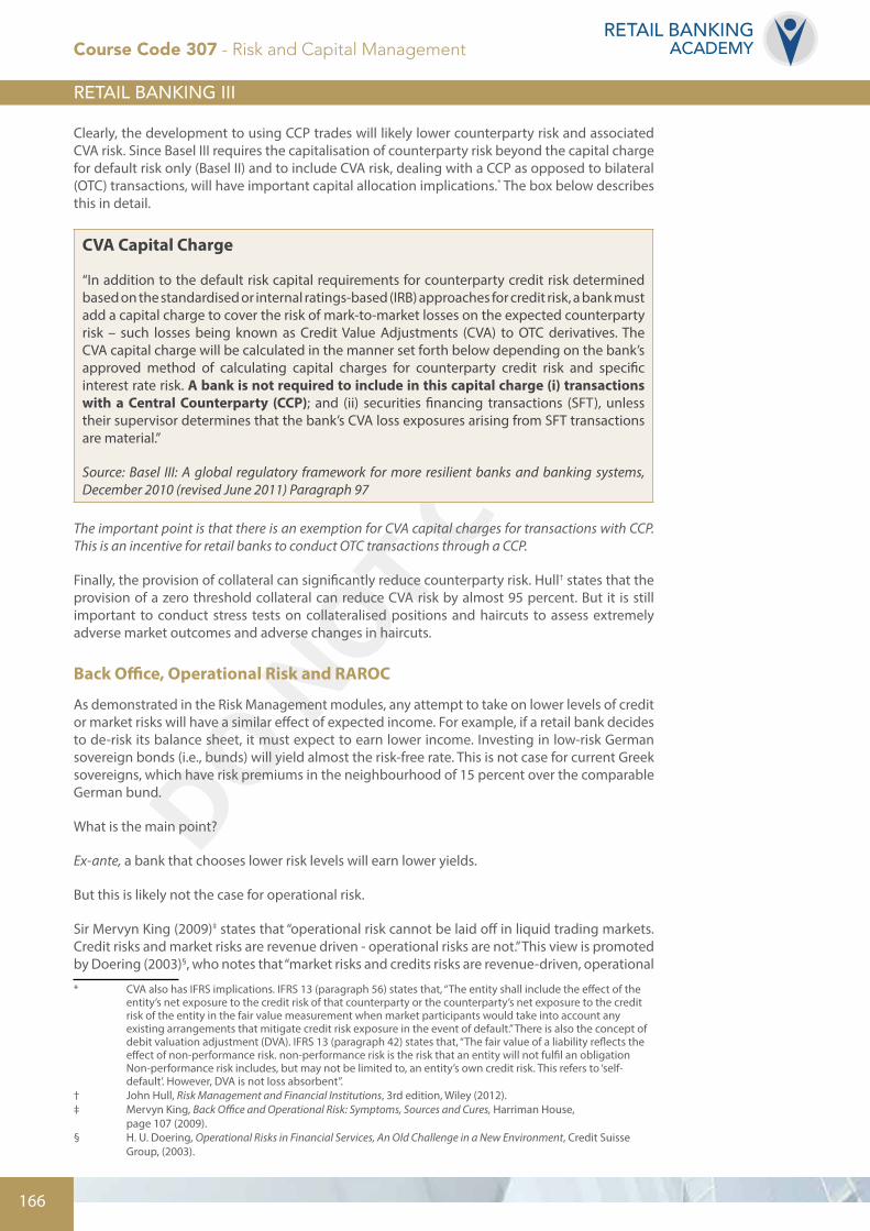
Clearly, the development to using CCP trades will likely lower counterparty risk and associated CVA risk. Since Basel III requires the capitalisation of counterparty risk beyond the capital charge for default risk only (Basel II) and to include CVA risk, dealing with a CCP as opposed to bilateral (OTC) transactions, will have important capital allocation implications.* The box below describes this in detail.

CVA Capital Charge

“In addition to the default risk capital requirements for counterparty credit risk determined based on the standardised or internal ratings-based (IRB) approaches for credit risk, a bank must add a capital charge to cover the risk of mark-to-market losses on the expected counterparty risk – such losses being known as Credit Value Adjustments (CVA) to OTC derivatives. The CVA capital charge will be calculated in the manner set forth below depending on the bank’s approved method of calculating capital charges for counterparty credit risk and specific interest rate risk. A bank is not required to include in this capital charge (i) transactions with a Central Counterparty (CCP); and (ii) securities financing transactions (SFT), unless their supervisor determines that the bank’s CVA loss exposures arising from SFT transactions are material.”

Source: Basel III: A global regulatory framework for more resilient banks and banking systems, December 2010 (revised June 2011) Paragraph 97

The important point is that there is an exemption for CVA capital charges for transactions with CCP. This is an incentive for retail banks to conduct OTC transactions through a CCP.

Finally, the provision of collateral can significantly reduce counterparty risk. Hull† states that the provision of a zero threshold collateral can reduce CVA risk by almost 95 percent. But it is still important to conduct stress tests on collateralised positions and haircuts to assess extremely adverse market outcomes and adverse changes in haircuts.

Back Office, Operational Risk and RAROC

As demonstrated in the Risk Management modules, any attempt to take on lower levels of credit or market risks will have a similar effect of expected income. For example, if a retail bank decides to de-risk its balance sheet, it must expect to earn lower income. Investing in low-risk German sovereign bonds (i.e., bunds) will yield almost the risk-free rate. This is not case for current Greek sovereigns, which have risk premiums in the neighbourhood of 15 percent over the comparable German bund.

What is the main point?

Ex-ante, a bank that chooses lower risk levels will earn lower yields.

But this is likely not the case for operational risk.

Sir Mervyn King (2009)‡ states that “operational risk cannot be laid off in liquid trading markets. Credit risks and market risks are revenue driven - operational risks are not.” This view is promoted by Doering (2003)§, who notes that “market risks and credits risks are revenue-driven, operational

* CVA also has IFRS implications. IFRS 13 (paragraph 56) states that, “The entity shall include the effect of the entity’s net exposure to the credit risk of that counterparty or the counterparty’s net exposure to the credit risk of the entity in the fair value measurement when market participants would take into account any existing arrangements that mitigate credit risk exposure in the event of default.” There is also the concept of debit valuation adjustment (DVA). IFRS 13 (paragraph 42) states that, “The fair value of a liability reflects the effect of non-performance risk. non-performance risk is the risk that an entity will not fulfil an obligation Non-performance risk includes, but may not be limited to, an entity’s own credit risk. This refers to ‘self- default’. However, DVA is not loss absorbent”.† John Hull, Risk Management and Financial Institutions, 3rd edition, Wiley (2012).‡ Mervyn King, Back Office and Operational Risk: Symptoms, Sources and Cures, Harriman House, page 107 (2009).§ H. U. Doering, Operational Risks in Financial Services, An Old Challenge in a New Environment, Credit Suisse Group, (2003).


DO NOT COPY



risks are not,” (page 11).

This comment by King implies that actions to reduce operational risk will not reduce revenues. Indeed, experts believe* that there is little recognition that operational risk is fundamentally different to market and credit risk in terms of:

• Expense versus income

• Being not dependent on risk appetite

• Major dependency on people and culture

But is operational risk a truly special risk?

We summarise current research findings on the special characteristics of operational risk compared to credit and market risks. We look at the arguments put forward in a group of research papers that operational risk is one-sided and firm-specific. We then expand on these two issues and provide counter-arguments.

First Issue: Operational Risk is One-Sided

a) Operational risk is different from credit risk and market risk in that it – operational risk – is a pure risk. Banks do not assume operational risk for profit. Indeed, this is different from credit risk and market risk where some risk is taken (see calculation of risk-weighted assets) in order to generate a risk premium.

This means that it is a one-sided risk. Herring (2002)† views operational risk as downside risk and cannot see how operational risk can deliver unexpected profit. This view is also supported by Lewis and Lantsman (2005)‡ who assert that there are only two states involved in operational risk – loss or no-loss. The loss may arise from systems failure (i.e., loss of business) or from people errors (i.e., monetary payout to address customer complaints). The other alternative is no loss. This is like an insurance risk. The insurance provider has two states to deal with. The first is no loss in that the insurable event (i.e., fire) did not occur. The second is a loss that leads to a monetary payout to the customer because the insured event occurred. There is no profit opportunity.

Second Issue: Operational Risk is Bank-Specific

b) Unlike market risk and credit risk, operational risk is idiosyncratic in the sense that it is bank- specific. The effects of operational failure are localised to that one bank, and do not spill over to other banks. This is quite different from credit risk in the recent sub-prime mortgage crisis that became a global problem arising mainly from securitisation – so-called mortgage-backed securities. In other words, there is no contagion effect and so, by extension, operational risk is not systematic§. This view is proposed by Lewis and Lantsman (2005) who, with respect to operational risk, stated, “the risk of loss tends to be uncorrelated with general market forces”. Presumably, operational risk is not related to the business cycle and operational failure, as measured by the frequency and severity of losses, is bank-related only. If this view is correct, then the implication is quite profound. Basel II regulation and capital requirements for operational risk are unnecessary. This conclusion is supported by Danielsson et al (2001).¶

* First Nigerian Annual International Conference On Operational Risk 2011 (22-23 February 2011).† R. J. Herring, “The Basel 2 Approach to Bank Operational Risk: Regulation on the Wrong Track”, Paper Presented at the 38th annual Conference on Bank Structure and Competition, Federal Reserve Bank of Chicago, (2002).‡ C. M. Lewis and Y. Lantsman, “What is a Fair Price to Transfer the Risk of Unauthorised Trading? A Case Study on Operational Risk”, in E. Davis, (ed) Operational Risk: Practical Approaches To Implementation, London: Risk Rooks (2005).§ There is an analogy to the beta risk of a stock which is correlated to the market index. The portion of total risk that is not systematic is called idiosyncratic or firm-specific.¶ J. Danielsson, P. Embrechts, C. Goodhart, C. Keating, F. Muennich, O. Renault and H.S. Shin, “An Academic Response to Basel II”, LSE Financial Markets Group, Special Paper No 130 (2001).


DO NOT COPY

168


A counterpoint

On the other hand, Moosa (2008) argues that operational risk is not unrelated to the state of the economy. For example, credit card fraud is pro-cyclical – it rises when consumer spending is rising, which itself is positively correlated with the growth of gross domestic product. The risk of rogue trading is higher when financial markets are rising, at which time volatility is also increasing. Chernobai et al (2007) also propose three reasons why operational risk is related to the economy. There are sound reasons why operational losses may be pro-cyclical and just as good reasons why they may be countercyclical (i.e., rise when the economy is weak and GDP growth is declining). For example, when unemployment rises during a downturn there may be more internal oversight, reducing potential operations risk – pro-cyclical.

But then employees who are expecting layoffs may slacken off, thereby increasing the likelihood of fraud and security breach – countercyclical.

Finally, as a rebuttal to the one-sided view of operational risk, Kilavuka (2008)* presents an example of ATMs as a fee-generation business but also a risky one in the sense that an expansion of the ATM network is subject to a higher likelihood of fraudulent activity. So there is a risk-return trade-off.

Here is another (compromise) view. In order to present it contextually, let us consider the Basel II definition of operational risk. The BCBS states:

The committee has defined operational risk as the risk of loss resulting from inadequate or failed internal processes, people and systems or from external events. This definition includes legal risk, but excludes strategic and reputational risk as well as ‘indirect losses’.

Banks have taken significant steps over the years to manage credit risk and market risk. They have developed complex modelling to implement internal ratings-based (IRB) methodology (foundation and advanced), and invested in sophisticated software and hardware assets to measure capital requirements. For market risk, Value at Risk modelling is preferred. But in doing this, they create operational risk – specifically, risks from failed internal processes.

When retail banks invest in assets – human, IT systems and databases – to calculate capital requirements for credit based on the Internal Ratings-Based methodology or VaR for market risk, there is a potential for operational risk in terms of unintentional human errors, failed systems and corrupted data. The assessment of credit risk and market risk may lead to operational risk.

In this sense, a retail bank does not take on operational risk. The bank takes on credit risk and market risk to generate expected profit. The bank calculates minimum capital requirements to support unexpected loss over a one-year time horizon. This normal banking business creates the potential for operational failure, as a consequence. So operational risk is one-sided. Operational risk has two states – loss or no loss. Unintentional human errors create additional cost of time and effort to correct the problem and communicate (probably via the legal department) with affected parties with appropriate apology or compensation. Failed internal systems lead to cost of repair and probably replacement investment. These are all instances of additional cost. There is no opportunity for revenue-generation.

But this is only in the short term.

A high frequency of low-severity events may not lead to significant additional costs, but can have a meaningful impact on the bank’s reputation. We examine this issue in some detail.

It is interesting that the Basel definition of operational risk does not include minimum capital requirements for reputation risk. In the BCBS (1998, page 7), reputational risk is described as “the risk of significant negative public opinion that results in a critical loss of funding or customers”.

* M Kilavuka: “Managing operational risk capital in financial institutions”, Journal of Operational Risk, Volume 3 Number 1, (Spring 2008).


DO NOT COPY



There are several reasons why internally generated operational failure may lead to loss of revenue.

Customers may lose trust in the bank. On the flip side, an erosion of trust may lead either to termination of existing business with the bank or a decision not to engage in new business. But this is a long-term effect. Erosion of trust will require more than one instance of human error or failed internal process.

The academic literature has provided evidence of a link from operational risk to reputational damage.* Finally, we agree with Moosa (2008)† that operational risk is not bank-specific and is correlated with economy-wide forces. This is because, in our view, operational risk is correlated with market risk and credit risk, each of which is correlated with the economy. Hence, the allocation of risk capital for operational risk by the BCBS is appropriate.

Gillet, Hubner and Plunus (2010) showed that in cases of “internal fraud, the loss in market value is greater that the operational loss amount announced, which is interpreted as a sign of reputational damage”. A similar result was obtained in a recent study on European banks.‡

* Gillet, Hubner and Plunus, “Operational risk and Reputation in the Financial Industry”, in Journal of Banking and Finance, Volume 34, issue 1, pages 224-235 (2010).† Moosa, IA, “Quantification of Operational Risk under Basel II: the Good, Bad and Ugly”, London: Palgrave (2008).‡ “Operational and Reputational Risk in the European Banking Industry: The Market Reaction to Operational Risk Events” by Philipp Sturm, 30 November 2010 (unpublished).


DO NOT COPY

170


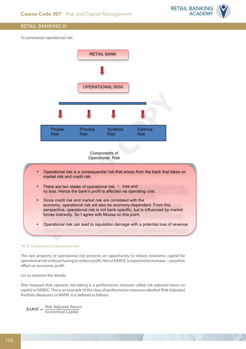
To summarise operational risk:

RETAIL BANK

People Process Systems External Risk Risk Risk Risk

Components of Operational Risk

• Operational risk is a consequential risk that arises from the bank that takes on market risk and credit risk.

• There are two states of operational risk –

loss and no loss. Hence the bank’s profit is affected via operating cost.

• Since credit risk and market risk are correlated with the

economy, operational risk will also be economy-dependent. From this perspective, operational risk is not bank-specific, but is influenced by market forces indirectly. So I agree with Moosa on this point.

• Operational risk can lead to reputation damage with a potential loss of revenue.

OPERATIONAL RISK

307.8: Components of Operational Risk

This last property of operational risk presents an opportunity to reduce economic capital for operational risk without having to reduce profit. Hence RAROC is expected to increase – a positive effect on economic profit.

Let us examine the details:

One measure that captures risk-taking is a performance measure called risk-adjusted return on capital or RAROC. This is an example of the class of performance measures labelled ‘Risk-Adjusted Portfolio Measures’ or RAPM. it is defined as follows:

Risk Adjusted Return Economical Capital

This property of operational risk presents an opportunity to reduce economic capital for

operational risk without having to reduce profit. Hence RAROC is expected to increase

– a positive effect on economic profit.

Let us examine the details:

One measure that captures risk-taking is a performance measure called risk-adjusted

return on capital or RAROC. This is an example of the class of performance measures

labelled ‘Risk-Adjusted Portfolio Measures’ or RAPM. It is defined as follows:

CapitalEconomicturnAdjustedRiskRAROC Re

= ,

where:

Risk-Adjusted Return =

• Operational Risk is a consequential risk that arises from the bank that takes on market risk and credit risk.

• In this sense, I share the view with several authors quoted in this chapter, that operational risk is one-sided. There are two states of operational risk – loss and no loss. Hence the bank’s profit is affected via operating cost.

• By my interpretation, since credit risk and market risk are correlated with the economy, operational risk will also be economy-dependent. From this perspective, operational risk is not bank-specific, but is influenced by market forces indirectly. So I agree with Moosa on this point.

• Operational Risk can lead to reputation damage with a potential loss of revenue.


DO NOT COPY



where:

Risk-Adjusted Return = Revenues – Operating Expenses – Expected Loss + Capital Benefit. It is actually expected profit adjusted for expected loss.

Economic Capital (or ECAP) is capital that is reserved as a buffer against unexpected loss for a given level of confidence (i.e., 99.5 percent) over one year. It is a cover for the risks (credit, market and operational risks) that are incurred by normal banking activities. The Economist (2003) defines economic capital as “the theoretically ideal cushion against unexpected losses”. Economic capital is depicted graphically as follows:

Probability of Loss

Expected Loss

Confidence Level

Economic Capital Amount of Loss

This graph shows that loss that is smaller than expected loss is more frequent. In

addition, actual losses higher than the expected loss are rare, but there is still a positive

probability of occurrence – it could still happen. This is a feature of a skewed distribution

with a right tail. The extremely rare event is situated in the tail of the loss distribution –

the so-called tail-risk. The confidence level is normally determined by the bank’s target

debt level. For example, a target debt level at AA implies that the probability area in the

tail is 0.05 per cent (5 basis points). The amount of economic capital is inferred from the

confidence level of 100 percent - 0.05 percent = 99.95 percent. Typical tail probabilities

are as follows:

307.9: Economic Capital

This graph shows that loss that is smaller than expected is more frequent. In addition, higher than expected losses are rare, but they can happen. This is a feature of a skewed distribution with a right tail. The extremely rare event is situated in the tail of the loss distribution – the so-called tail-risk. The confidence level is normally determined by the bank’s target debt level. For example, a target debt level at AA implies that the probability area in the tail is 0.05 percent (5 basis points). The amount of economic capital is inferred from the confidence level of 100 percent - 0.05 percent = 99.95 percent.

Typical tail probabilities are as follows:

Debt rating (Standard and Poor’s) Maximum probability of default (typical basis points)

AAA 1.5

AA 5

A 6

BBB 20

Some further points of clarification are useful.

Actual loss may deviate from the expected loss that is predicted by bank experts, based on historical experience. If the actual loss is less than the expected loss, the amount that was provisioned turned out to be too high and is typically carried over to the next accounting period. But, if the actual loss is more than the amount that was provisioned, then available capital will buffer this negative deviation.


DO NOT COPY

172


Summary

Economic Capital is the amount of capital required to cover unexpected loss (i.e., actual loss beyond the expected loss that is predicted by banking executives).

Recall the main point stated above: the one-sided view of operational risk implies two states of existence – a loss occurring arising from people, process or systems failure or no loss at all. If management takes action to mitigate operational risk, then ex post, there will be a reduction in operational cost and an increase in profits. It is also likely that the ex-ante allocation of economic capital to account for operational risk will be less after the fact. There will also be a positive effect on RAROC.

We now consider the capitalisation for operational risk at IRB banks.

Operational Risk

Module 209 has covered the standardised and basic indicator approaches to calculate the capital charge for standarised banks. There is also a preliminary discussion of the IRB approaches that is called the Advanced Measurement Approaches (AMA) that requires the calculation of a capital charge to a 99.9 percent confidence level over a one-year holding period. We develop the two AMA approaches in greater detail in this section.* It is noted that banks may use the standardised or basic approaches for some (presumably) less complex part of its operations.

To ensure continuity, we briefly review the Basic Indicator and Standardised Approaches.

Basic Indicator Approach (BIA)

This approach is simple to implement, and probably does not properly measure operational risk – likely only indirectly.

The bank’s required operational risk capital = alpha * (average gross income of the three previous years where in calculating this average, adjustments made to both the numerator and denominator for negative and zero values).

First alpha = 15 percent is a fixed percentage set by BCBS. Also if the bank earned zero or negative gross income for a particular year, the sample value is omitted from the denominator and numerator. This means that if the gross income for one of the past three years is negative, the average is taken over the two years with positive gross income values.

So if the average three-year gross income for a bank (assuming all positive values) is $50m, the capital that will be allocated for operational risk is 15% * $50m = $7.5m.

The main problem with the BAI is that it assumes that the bank with a higher average of gross income will experience higher operational risk – in a fixed proportional manner. This can be misleading since operational risks depend on the type of business that a bank engages in. A bank may have a relatively lower average of gross income and yet have a relatively higher level of operational risk.

The Standardised Approach

The standardised approach is similar to the BIA, except that SA deals with lines of business rather than the bank’s gross revenue as whole. The standard approach recognises that operational risk varies by business unit.

* There is also a third approach based on a balanced scorecard


DO NOT COPY



Here is a table of beta factors for each line of business:

Business unit Beta factor (fixed percentage)

Corporate finance 18%

Payment and settlement 18%

Trading and sales 18%

Agency services 15%

Commercial banking 15%

Asset management 12%

Retail banking 12%

Retail brokerage 12%

The AMA approaches require supervisory approval and substantial IT capability with a robust and reliable database that not only stores internal data, but can integrate data from external sources.

The Internal Measurement Approach (IMA)

A relatively detailed discussion of IMA is provided in Module 209. We quickly review it to highlight its complexity and the huge amount of data that is required. This will serve to rationalise why banks seem to prefer the Loss Distribution Approach (LDA).

The IMA is based on a procedure that is described as follows:

a) Consider a matrix that is based on a business line–event type combination. The Basel Accord uses a business line-loss event type matrix to identify potential operational losses. The columns are business lines while the rows are Basel’s seven categories of loss event types. These event types are: (1) internal fraud; (2) external fraud; (3) damage to physical assets; (4) business disruption and systems failures; (5) client, products and business services; (6) execution delivery and management processes; and (7) employment practices & work safety. The expected loss amount for each cell in this matrix (ELAi,j) for each business line (i) and each loss event identified from internal loss data (j) is calculated according to the relationship:

ELAi, j = EIi, j ×PEi, j × LGEi, j


DO NOT COPY

174


Here is a diagrammatic representation:

LOB1 LOB2 LOB3 LOB4 LOB5 LOB6 LOB7 LOB8

Event 1

Event 2

Event 3

Event 4

Event 5

Event 6

Event 7

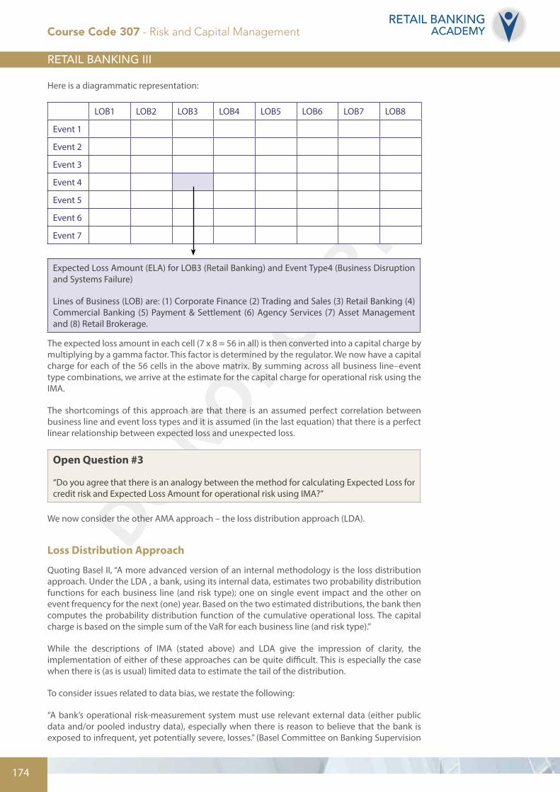
Expected Loss Amount (ELA) for LOB3 (Retail Banking) and Event Type4 (Business Disruption and Systems Failure)

Lines of Business (LOB) are: (1) Corporate Finance (2) Trading and Sales (3) Retail Banking (4) Commercial Banking (5) Payment & Settlement (6) Agency Services (7) Asset Management and (8) Retail Brokerage.

The expected loss amount in each cell (7 x 8 = 56 in all) is then converted into a capital charge by multiplying by a gamma factor. This factor is determined by the regulator. We now have a capital charge for each of the 56 cells in the above matrix. By summing across all business line–event type combinations, we arrive at the estimate for the capital charge for operational risk using the IMA.

The shortcomings of this approach are that there is an assumed perfect correlation between business line and event loss types and it is assumed (in the last equation) that there is a perfect linear relationship between expected loss and unexpected loss.

Open Question #3

“Do you agree that there is an analogy between the method for calculating Expected Loss for credit risk and Expected Loss Amount for operational risk using IMA?”

We now consider the other AMA approach – the loss distribution approach (LDA).

Loss Distribution Approach

Quoting Basel II, “A more advanced version of an internal methodology is the loss distribution approach. Under the LDA , a bank, using its internal data, estimates two probability distribution functions for each business line (and risk type); one on single event impact and the other on event frequency for the next (one) year. Based on the two estimated distributions, the bank then computes the probability distribution function of the cumulative operational loss. The capital charge is based on the simple sum of the VaR for each business line (and risk type).”

While the descriptions of IMA (stated above) and LDA give the impression of clarity, the implementation of either of these approaches can be quite difficult. This is especially the case when there is (as is usual) limited data to estimate the tail of the distribution.

To consider issues related to data bias, we restate the following:

“A bank’s operational risk-measurement system must use relevant external data (either public data and/or pooled industry data), especially when there is reason to believe that the bank is exposed to infrequent, yet potentially severe, losses.” (Basel Committee on Banking Supervision


DO NOT COPY



[BCBS], 2006, Paragraph 674.)

By its name, this approach combines two distributions. The first is a discrete distribution of the frequency of losses. The second is a continuous distribution of the severity of losses.

But before we describe the LDA procedure in more detail, we emphasise that loss data from the bank’s internal database (as well as from external sources) have inherent weaknesses. First, Loss data is backward looking and, importantly, there is likely not enough loss data to properly capture loss distributions – especially the tails of these distributions.

Hence, apart from ensuring that the bank internal data base is robust, we note that this may be augmented by external (consortium) data sources. These include:

• Global Operational Loss Database (GOLD) of the British Bankers’ Association (BBA). It is noteworthy that in 2005, GOLD is congruent with the definitions of business lines-loss event types that are stated above in the application of IMA.

• Operational Riskdata eXchange (ORX). This is a forum for the exchange of operational risk-related loss information in a standardised, anonymous and quality assured form. Members include: ING, BNP Paribas, JP Morgan, Deutsche Bank, Bank of America, the Bank of Nova Scotia, and Banca Intesa.

Open Question #4

“‘Data! Data! Data!’ [Sherlock Holmes] cried impatiently. I can’t make bricks without clay.” (Arthur Conan-Doyle, “The Adventure of the Copper Beeches”)

How might this apply to the implementation of AMA approaches?

The LDA approach is consistent with obtaining a VaR estimate for operational risk (the so-called OP VaR).

The convolution of the frequency and severity of distributions to create the total loss distribution is represented below:


DO NOT COPY

176


Counterparty A

Pays Fixed

Pays LIBOR

Counterparty BCCP

Pays Fixed

Pays LIBOR




=Probability

OP VaR (α)

α = 0.1%


Counterparty A

Pays Fixed

Pays LIBOR

Counterparty BCCP

Pays Fixed

Pays LIBOR




=Probability

OP VaR (α)

α = 0.1%


307.10: Total loss distribution

Comment

In contrast to regulatory capital for credit risk for corporate loans, banks that use the AMA approach may have to set aside capital for both expected and unexpected operational losses – the full OP VaR Value.

Market Risk*

Module 209 covers the basics of the Internal Measurement Approach (IMA) Market Risk VaR. It is based on a 99 percent confidence level over a 10-day holding period and calculation is done on a daily basis. Data sets are updated at least once per month and are based on historical observations for at least one year.

The new minimum trading book capital comprises a 10-day 99 percent VaR and a stressed VaR which was introduced during Basel 2.5 and it is also a 10-day 99 percent VaR but uses a 12-month observation period during a crisis. There is also an incremental risk charge (IRC). This is risk charge that is expected to capture default risk and credit migration risk for non-securitisation exposures

* According to BCBS June 2006 (par 683): “Market risk is the risk of losses in on-and off-balance sheet positions arising from movement in market prices. Market risks arise from instruments in the trading book (e.g., interest rate risk and equity risk) and throughout the institution (e.g., foreign exchange risk and commodities risk. Note that derivative transactions are subject to both market risk and counterparty credit risk capital requirements)”.


DO NOT COPY



over a one-year horizon at 99.9 percent. these two risks are incremental to the risks captured by the normal VaR over a 10-day horizon at a 99 percent confidence interval. Note that IRC is similar to CVA in intent but CVA applies to counterparty risk.

We conclude this module with a discussion of risk governance.


DO NOT COPY

178


Chapter 4: Risk Governance

Firstly, we note that corporate governance involves the allocation of authority and responsibilities within the bank so senior management and the board of directors can set business strategy and objectives, determine the bank’s risk tolerance and ensure that all stakeholder interests are taken into account and that the bank’s activities are lawful and in accordance with ethics and integrity.

This shows that risk governance is part of corporate governance. Indeed, risk governance may be defined as “an integrated framework laid out to provide guidance for comprehensive assessment and management of risks”. An effective risk governance framework ensures that the firm is able to achieve its stated goals within the chosen risk appetite framework.

Why is risk governance important in banks?

Here is a response to this question by Anand Sinha, Deputy Governor of the Reserve Bank of India, at the Risk & Governance Summit, organised by the Indian School of Business and Deloitte, in Mumbai, 23 August 2012.

“Banks are special. In their role as intermediaries, they perform a critical function of risk transformation which results in warehousing of risks by banks. Further, banks’ business model of accepting deposits for lending, leads to significant leverage (a leverage of about 18 times that of banks, during 1995–2010, against the leverage of three times that of non-financial firms). Liquidity risks can be critical even for well capitalised banks, a lesson the global crisis has emphatically demonstrated.

“The banking business has become far more sophisticated and complex. Risk too, has increased in proportion to this sophistication and complexity. The risk-taking behaviour of banks has high potential for contributing to and amplifying systemic risk and consequent contagion. This can have severe repercussions for financial and economic fragility as witnessed during and in the aftermath of the global financial crisis.

“Given their unique business model and also the special role played in the financial system, sound internal governance for banks is essential, requiring Boards to focus even more on assessing, managing, and mitigating risk. Banks operate on the foundation of public confidence and any small breach in that confidence can lead to a run on the bank and to an eventual failure.”


DO NOT COPY



What measures are needed to create effective risk governance?

In addition to prescribing the risk appetite for the institution, the board also needs to lay down appropriate risk strategy and ensure that this is institutionalised throughout the organisation. This would entail aligning risk management processes with the overall business strategy, clearly defining the roles and responsibilities down the hierarchy, establishing accountability and reinforcing change with communication and training.

The board and the senior management oversight must be supplemented with effective leadership by the Chief Executive Officer (CEO). The boards must get more intimately involved in risk matters and have a firmer understanding of the key risks faced by the business.

Effective risk governance also demands that each director is aware of the breadth of risks faced by the bank. Directors add value to the board when they have financial expertise, are aware of risk fundamentals and techniques, and are able to manage dynamics with executives.

A board level risk committee has an important role to play in the overall risk governance framework. Apart from monitoring the firm’s strategic risk profile on an ongoing basis, such a committee would also be responsible for defining the firm’s overall risk appetite; approving major transactions above agreed risk thresholds, and establishing limit structures and risk policies for use within individual businesses.

Presence of a Chief Risk Officer (CRO) is expected to strengthen the executive risk management framework. However, independence of the CRO, with necessary stature to influence decisions, would be a critical element in ensuring the effectiveness of the post in risk management processes and also the strategic risk management-related decisions. The CRO must report directly to the CEO and the board and be responsible for all risks, risk management and control functions.

Another important requirement is integrating risk with business strategy and compensation. Risk – and return on risk – need to be a core component of any performance measure, and should be explicitly factored into incentive and compensation schemes. Compensation must be formally aligned with actual performance, such as adding more rigorous risk-based measures to scorecards. This would also involve moving to longer vesting periods, and increasing deferred compensation.

Here is some advice from Governor Randall S Kroszner, delivered at the Global Association of Risk Management Professionals Annual Risk Convention, in New York, on 25 February 2008:

“To ensure sound risk management, boards of directors and senior management at financial institutions must also establish an overall governance and control structure that is credible, robust, and consistent throughout the firm. It is critical that senior management set the tone at the top, communicate it, and lead by example. This strategy should be clearly articulated and should be recognisable in the actions of the firm’s employees. Business lines should be held equally accountable and there should not be any special treatment for ‘star’ employees, even if they are bringing sizable revenues into the institution in a particularly year.

“All senior managers would benefit from taking a fresh look at the incentive structures within their firm. For example, are all parties being compensated on a risk-adjusted basis that takes into account longer-term performance? Is management able to determine how risk taking at the business-unit level affects firm-wide risks? Do business units have the right incentives to consider their units’ risk taking in the context of the entire institution? These and other questions deserve attention, given some of the risk-management challenges seen lately. But I am confident that the industry can find appropriate solutions, and supervisors will assist them in those efforts.”


DO NOT COPY

180


Risk Appetite Framework (RAF)

The Risk Appetite Framework comprises a Risk Appetite Statement (RAS) with supporting risk metrics that cascade into risk limits at the operational level. While there is still ambiguity in risk terminology in the banking literature, the Financial Stability Board (FSB) paper titled ‘Thematic Review on Risk Governance’ has made substantial progress in arriving at a consensus in relation to terminology used in risk governance. Based on this report and others in the extant literature, the following definitions with explanations are presented.

a) Risk capacity (also called, risk-bearing capacity) is the maximum level of risk the firm can assume before breaching constraints determined by regulatory capital and liquidity requirements and its obligations to stakeholders. Simply put, risk capacity represents the bank’s ability to bear risk and it is determined by the bank’s resources – available capital, liquidity, people skills and experience, risk culture and operational processes and IT infrastructure. In consideration of financial capacity from a regulatory perspective, banks typically measure their risk capacity in terms of the book value of equity with adjustments for such items as intangible assets (including goodwill), deferred tax assets, revaluation reserves etc. Arguably, a more conservative measure is regulatory Tier 1 capital. A recent report by McKinsey & Company (Mastering ICAAP, May 2011) indicates that eighty-five percent of banks in their sample associate risk-bearing capacity with Tier 1 capital.

It is common for banks to conduct quarterly stress tests on its aggregate risk-bearing capacity under severe conditions. Such scenarios include a significant deterioration of global macroeconomic conditions, above-average interest rate volatility and a significantly increased risk of corporate failure. But risks are typically correlated. A political crisis in the country cannot only have significant negative effects on the bank’s loan portfolio but may at the same time lead to currency devaluation and extremely high interest rate volatility. Consequently, banks should consider scenarios that go beyond historical experience – the latter being a statistical approach

b) Risk appetite or tolerance is a specific determination of the amount of risk that a bank is willing to take in its effort to earn profit. It should reflect the bank’s business strategy and profitability expectations and hence it is forward-looking.

Specifically, a bank’s risk appetite reflects the aggregate level as well as the types of risk it is willing to assume to achieve its business strategy. Importantly, a bank’s risk appetite should be constrained by its risk-bearing capacity to allow for shortcomings in statistical models and for adverse effects of non-quantitative risks not explicitly included in risk capacity models

The bank’s risk appetite statement typically includes risk metrics such as: capital adequacy target; target debt level; target and maximum asset to equity ratio; loan portfolio concentration limit; and target and maximum loan to deposit ratio. In addition, the RAS should include qualitative statements in relation to regulatory compliance, reputational impact, fraud incidence, ethical violations etc. These statements should indicate which risks the bank is not willing to take and why.

But a RAS must cascade into specific processes that can be implemented and monitored at the ‘desk level’. This means that the RAS which is formulated by the board of directors and senior management must be translated into clear risk limits. A risk trigger or warning limit is a warning signal that requires review of the risk level by management and/or the board. A risk limit reflects a level of exposure for the bank that should not normally be exceeded. Should risk limits be breached then this will trigger a corrective management action. It is like a red light. For example, in the case of credit and counterparty risk, limits may be placed on exposures for a country/industry/product segments/specific obligor. Such limits will have implications for portfolio diversification and concentration risk. Similarly, for liquidity risk, a limit may be placed on the minimum level of liquid assets.


DO NOT COPY



Risk limits should be set at a level to constrain risk-taking within risk appetite based on an estimate of the impact on the interests of customers (e.g. depositors, policyholders) and shareholders, as well as capital and other regulatory requirements, in the event that a risk limit is breached and the likelihood that each material risk is realised (FSB, Principles for an Effective Risk Appetite Framework, 17 July, 2013)

In other words, they put a brake on excessive risk-taking.

The RAS is dynamic reflecting the risk appetite over time. Hence as the bank’s economic environment evolves and different strategies are adopted, the RAS must be updated and risk limits and risk appetite/tolerance modified.

Here is an example illustrating risk limits and risk trigger limits for the bank’s loan to deposit ratio (LTD).

Exposure

Time

Risk Limit: LTD = 110%

Trigger Limit: LTD = 100%

Lower Limit: LTD = 80%

Actual risk exceeds risk trigger limit;

this is a warning signal

Actual risk level exceeds

risk limit;this is a red

light. Reduce risk exposure

to within limits

Actual risk is below risk

limit; review if it is too low

and should be managed

307.11: Risk limits and risk trigger limits for LTD

In this example, the RAS translates into a loan to deposit ratio in the range of 80% to 110%. In the case where the leverage ratio is above the 100% risk trigger limit but below the risk limit of 110%, management must consider taking steps to reduce this ratio down below 100%. It is a warning signal. When the LTD ratio exceeds the risk limit of 110% in this case, there is a red alert and steps must be taken as soon as possible to reduce this ratio – for example, reduce loan portfolio or increase deposits. The final case is where the LTD is below the lower risk limit. It signals that the aggregate level of risk in the loan portfolio is too low and bank management should consider increasing lending.

Note however that not all risks are quantifiable and therefore amenable to risk limits/tolerances. Qualitative risks such as strategic business risk and reputational risk are mitigated through incident management and oversight and control by experts in the bank.

In summary, risk governance is based on a three step process.

Definition of the bank’s risk appetite statement includes:

Step 1: Formulate risk principles


DO NOT COPY

182


Step 2: Cascade the risk appetite statement into risk limits for each risk type per business unit

Step 3: Governance of risk policies and monitoring risk limits

We conclude this discussion with an actual risk appetite statement for a Canadian bank. Modifications are made to protect confidentiality of this document.

Step 1: Risk Principles

Our reputation is paramount. We intend to be client advocates and to differentiate ourselves relative to our competitors in this way. We focus on those business risks that impact the customer experience.

Due to the importance of technology to our business, an operational risk culture relating to technology that tolerates only very low risks. For other operational risk areas, increased risk must be balanced against the need for efficiency in operations.

We seek to maintain a balance between mission, risk and return and to generate capital consistently through retained earnings that allow us to be self-sufficient.

Step2: Risk Limits

The risk to our capital is intended to be low.

We distinguish risks between near-term earnings at risk and long-term or stress events that could affect capital or solvency.

We will permit limited variations in earnings at risk but we have very low tolerance for losses that could potentially affect our solvency.

Limitations are placed on:

a) Bottom line Earnings at Risk due to moderate changes in interest rates in any given year of [25%] relative to the MTP forecast

b) The bank’s Tier One Capital Ratio, which will not fall below 10% of Risk Weighted Assets following an extreme event

c) Bank’s leverage ratio (Tier One Capital/Assets) will be no lower than 4%

d) The level of liquidity on hand, which will be sufficient to fund deposit outflows for three months during a stress event.

e) The ratio of Risk Weighted Assets to Total Assets, which will be below the median for major Canadian banks

The bank will rebuild its capital buffer after a stress event within two years through retained earnings, a reduction in the size of the balance sheet and/or accessing capital markets.


DO NOT COPY



Step 3: Governance – of risk policies and monitoring risk limits

Our risk governance process is based on the above principles and is implemented through a management risk culture, formalised with management risk committees and supplemented with risk limits.

The board of directors is responsible for safeguarding the interests of clients, shareholders and other stakeholders of the bank. The board reviews, discusses and approves the bank’s strategic plans which take into account the opportunities and risks of the business. The board is required to satisfy itself about the liquidity, funding and capital needs of the bank and ensures implementation of appropriate policies and systems to manage these needs. The board is also tasked with identifying the principal risks of the business and satisfies itself as to the implementation of appropriate systems to manage these risks. The board’s responsibilities include setting out the risk tolerance of the Bank by establishing financial limits as well as operational risk boundaries.

The bank’s risk framework is predicated on the three-lines-of-defence model. Within this model, business management (the first line) is responsible for developing and implementing controls to manage business risks while the risk specialist functions (the second line) have responsibility for translating the business risk appetite into methodologies and policies to support and monitor business management’s control of risk. Corporate Audit Services (the third line) provides independent assurance that control objectives are achieved by the first and second lines of defence.

The Chief Executive Officer is directly accountable to the board for the bank’s risk-taking activities. The CEO is supported by the organisation, the Executive Committee (EC), the senior management committees, the Risk Management department and the Legal and Compliance department.

The Chief Risk Officer provides oversight of the process to manage assets, liabilities, capital and associated risks. The CRO assesses and ensures the effectiveness of the systems and procedures that are used to identify, measure, monitor and report the bank’s risk exposures. The CRO reports to the CEO and functionally to the Chairman of the Risk Committee of the board of directors regarding the bank’s risk-taking activities.

The risk limit structure is developed and proposed by the CRO with management and approved by the board of directors. It is revised at least annually, as business conditions and risks evolve.

New business approval includes requiring each new business to propose a risk budget (including earnings at risk) and risk limits to be approved by the CRO and the CEO. Risk limits will be more conservative in newer product lines. Assumptions about risks will be made explicitly and metrics for risk and performance developed and tracked. Risk limits will be reviewed at least annually


DO NOT COPY

184


To summarise the key issues raised by BCBS and other commentators (see above, for examples) with respect to risk governance:*

BOARD Approves and oversees the firm’s risk appetite framework, including: the risk appetite statement (RAS), risk limits by business units consistent with the RAS, and policies and processes to implement the risk management framework

AUDIT COMMITTEE Oversees the review of the independent assessment of the risk governance framework

CRO•Develops risk metrics to reflect RAS•Monitors and reports on risk metrics•Escalates breaches of risk metrics•Conducts stress tests

307.12: Risk governance procedure

Summary

This module presented advanced methods for managing interest rate risk and liquidity risk, the two main dimensions of Asset Liability Management (ALM). In particular, we showed how to manage a duration gap with interest rate swaps as well as the impact of negative convexity on residential MBS and on callable bonds in general. The treatment of liquidity risk management complements the extensive coverage in the risk management module of Retail Banking II. We considered capital allocation methods for (internal-ratings based) IRB banks with emphasis on credit risk for retail exposures. The Loss Distribution Approach (LDA) is emphasised for operational risk. Capital allocation for counterparty risk with Credit Valuation Adjustment (CVA) is considered for both Over The Counter (OTC) and Central Counter Party (CCP) transactions. We also dealt with the central issues in risk governance that complements the Governance and Ethics module. Appendix I is a summary of relevant formulae that are applied in this module and Appendix II comprises the BCBS stress testing methodology for bank balance sheets.

* FSB: Thematic Review on Risk Governance


DO NOT COPY



Multiple Choice Questions

1. If an IRB formula produces a 4% capital requirement on a $1million dollar exposure, what is the dollar amount of the risk-weighted asset?

a) $40,000 b) $500,000c) $1 million d) $400,000

2. Under Foundation IRB, the supervisor provides estimates of three of the following. Which is the exception?

a) Exposure at Defaultb) Loss Given Defaultc) Probability of Defaultd) Maturity Adjustment

3. Which of the following is included in market risk charge?

a) Market riskb) Credit risk c) Operational riskd) Strategic business risk

4. In the Internal Measurement Approach (IMA) approach to calculate operational risk charge, which statement is incorrect?

a) The IMA approach assumes that there are seven lines of businesses.b) The IMA approach assumes that there are eight different event types.c) The capital charge is based on a fixed percentage of the average gross income over the last three years.d) The IMA approach assumes a linear relationship between expected loss and unexpected loss.

5. The balance sheet of a bank shows the following: Interest-earning Assets =$10 billion with duration = 6 years; Interest-bearing Liabilities = $8 billion with duration = 5 years. Based on this information, which one of the following statements is correct?

a) The bank’s liabilities are more interest rate sensitive than its assets.b) The duration gap is 2.5 years.c) The bank is currently exposed to rising interest rates.d) The bank is currently hedged against interest rate risk.

6. Traditional approaches try to reduce the duration gap to zero so as to stabilise shareholders’ equity in regard to interest rate risk. These approaches may be ineffective because they fail to:

a) ensure that convexity is zero.b) ensure that convexity is positive.c) mitigate credit risk before trying to reduce the duration gap to zero.d) modify duration by use of interest rate swaps.


DO NOT COPY

186


7. Residential mortgage-backed securities typically exhibit:

a) negative convexity at low yieldsb) negative convexity at high yieldsc) positive convexity at low yieldsd) negative convexity at all yields

8. Which statement is incorrect?

a) Counterparty risk is different from typical credit which is also called issuer risk.b) Credit Valuation Adjustment (CVA) applies to counterparty risk.c) A capital charge is required for counterparty risk for all transactions including those conducted through a central counterparty (CCP).d) The provision of collateral will reduce counterparty risk.

9. In relation to risk governance, which of the following approves and oversees the bank’s risk appetite framework (RAF)?

a) Senior Managementb) Chief Risk Officerc) Audit Committeed) Board of Directors

10. Which statement is incorrect?

a) An advantage of stress testing for banks is that it highlights the potential for extreme losses in banks’ portfolios.b) A monitoring tool for liquidity risk proposed by Basel III is ‘contractual maturity mismatch’.c) Level 2B assets must be no more than 40% of total high quality liquid assets.d) An advantage of stress testing is that it can help to overcome the shortcomings of the commonly used VaR model.

Answers:

1 2 3 4 5 6 7 8 9 10

b c d c c b a c d c


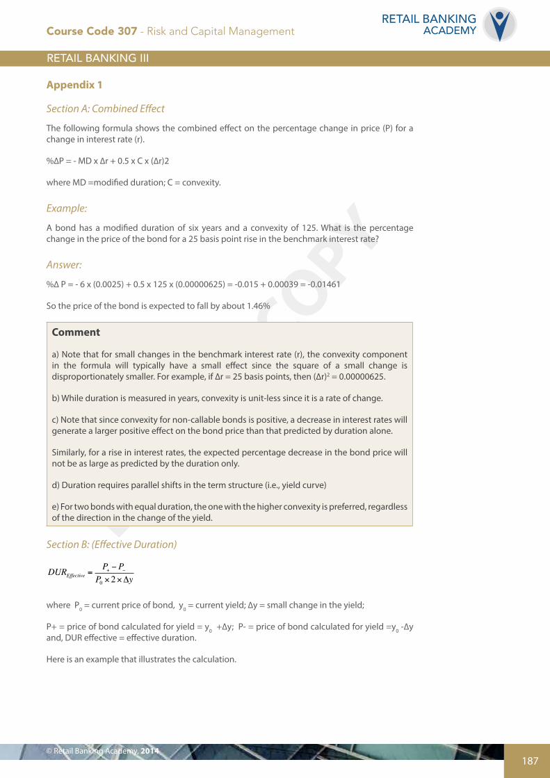
DO NOT COPY



Appendix 1

Section A: Combined Effect

The following formula shows the combined effect on the percentage change in price (P) for a change in interest rate (r).

%∆P = - MD x ∆r + 0.5 x C x (∆r)2

where MD =modified duration; C = convexity.

Example:

A bond has a modified duration of six years and a convexity of 125. What is the percentage change in the price of the bond for a 25 basis point rise in the benchmark interest rate?

Answer:

%∆ P = - 6 x (0.0025) + 0.5 x 125 x (0.00000625) = -0.015 + 0.00039 = -0.01461

So the price of the bond is expected to fall by about 1.46%

Comment

a) Note that for small changes in the benchmark interest rate (r), the convexity component in the formula will typically have a small effect since the square of a small change is disproportionately smaller. For example, if ∆r = 25 basis points, then (∆r)2 = 0.00000625.

b) While duration is measured in years, convexity is unit-less since it is a rate of change.

c) Note that since convexity for non-callable bonds is positive, a decrease in interest rates will generate a larger positive effect on the bond price than that predicted by duration alone.

Similarly, for a rise in interest rates, the expected percentage decrease in the bond price will not be as large as predicted by the duration only.

d) Duration requires parallel shifts in the term structure (i.e., yield curve)

e) For two bonds with equal duration, the one with the higher convexity is preferred, regardless of the direction in the change of the yield.

Section B: (Effective Duration)

DUREffective =P+ −P−

P0 ×2×Δy

where P0 = current price of bond, y0 = current yield; ∆y = small change in the yield;

P+ = price of bond calculated for yield = y0 +∆y; P- = price of bond calculated for yield =y0 -∆y and, DUR effective = effective duration.

Here is an example that illustrates the calculation.


DO NOT COPY

188


Example:

Consider a callable bond that pays 6% coupon with a four-year maturity that is currently selling at $102. The bond will be called at its par value of $100. Based on a Monte Carlo simulation, the

estimated price for a decrease in the current yield by 25 basis points is $102.3 while the estimate price for a similar increase in yields is $101. From this information, we can estimate the effective duration as follows:

P0 = $102; P+ = $102.5; P- = $101; ∆y = 25 basis points = 0.0025. Substituting into the formula for effective duration gives a value

Section C: Stability of Equity

If we incorporate the role of convexity but still assume that the change in average asset yield = change in average liability yield, then we obtain:

ΔE = −(DURA −LA×DURL )× A×Δr + 0.5(CA −

LA×CL )× A× (Δr)

2

Duration Gap Convexity Gap

Section D: A General Approach

Now we relax the likely unrealistic assumption that the average rate of asset yield is equal to average liability yield.

Assume that the benchmark interest rate changes by ∆r and the resulting average asset and liability yield changes as follows: Δra = βaΔr and Δrl = βl Δr. This means that if the benchmark rate changes by one percent, the average asset yield changes in some proportion of one percent which can be different from the response of the average liability yield. One can think of the beta coefficients as reflecting the sensitivity of asset or liability yield changes to changes in the benchmark rate. We assume that each beta value is higher than zero. For example, if βa = 80% , then if the benchmark yield is expected to increase by 1%, the asset yield is expected to increase by 80% of one percent or 80 basis points.

Clearly, only if βa = βl , we are back to the traditional assumption of equality of changes in both yields.

In this case the duration gap is calculated as follows:

DURGAP = DURA ×βa −LA⎛

⎝⎜

⎞

⎠⎟×DURL ×βl

Clearly the duration gap is zero and shareholders’ equity is immunised against interest rate changes if the following relationship holds:

DURA

DURL

=L×βlA×βa


102.5 - 101 102 x 2 x 0.0025

= 2.94

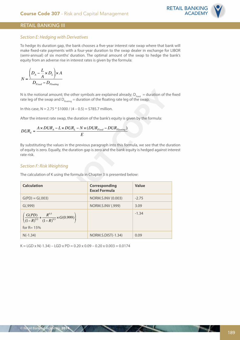
DO NOT COPY



Section E: Hedging with Derivatives

To hedge its duration gap, the bank chooses a five-year interest rate swap where that bank will make fixed-rate payments with a four-year duration to the swap dealer in exchange for LIBOR (semi-annual) of six months’ duration. The optimal amount of the swap to hedge the bank’s equity from an adverse rise in interest rates is given by the formula:

N =DA −

LA×DL

⎛

⎝⎜

⎞

⎠⎟× A

DFixed −DFloating

N is the notional amount; the other symbols are explained already; Dfixed = duration of the fixed rate leg of the swap and Dfloating = duration of the floating rate leg of the swap.

In this case, N = 2.75 * $1000 / (4 – 0.5) = $785.7 million.

After the interest rate swap, the duration of the bank’s equity is given by the formula:

DURE =A×DURA − L×DURL − N × (DURFixed −DURFloating )

E

By substituting the values in the previous paragraph into this formula, we see that the duration of equity is zero. Equally, the duration gap is zero and the bank equity is hedged against interest rate risk.

Section F: Risk Weighting

The calculation of K using the formula in Chapter 3 is presented below:

Calculation Corresponding Excel Formula

Value

G(PD) = G(.003) NORM.S.INV (0.003) -2.75

G(.999) NORM.S.INV (.999) 3.09

G(PD)(1− R)0.5

+R0.5

(1− R)0.5×G(0.999)

⎛

⎝⎜

⎞

⎠⎟

for R= 15%

-1.34

N(-1.34) NORM.S.DIST(-1.34) 0.09

K = LGD x N(-1.34) – LGD x PD = 0.20 x 0.09 – 0.20 x 0.003 = 0.0174


DO NOT COPY

190


Section G: Intuition on Capital Formula for Retail Exposures

An intuitive explanation of the formula for retail exposures is presented in Section F above. It is an intuitive explanation although the math may look intimidating.

An Intuitive Explanation of the IRB Formula for Retail Exposures

Here is the formula:

K = LGD×N G(PD)(1− R)0.5

+R0.5

(1− R)0.5×G(0.999)

⎛

⎝⎜

⎞

⎠⎟− LGD*PD

K = Cred VaR – EL

Credit VaR EL

The first part of the formula is Credit VaR (for 99% confidence for one year);

The second part of the formula is the expected loss (EL).

By subtracting, we get the unexpected loss (UL) for 99% over one year.

Capital is allocated for unexpected loss (K).

If we then multiply K by EAD, we get the capital charge.

Section H: Duration and Convexity

Useful Properties of Convexity:

a) For a zero-coupon bond, the Macaulay duration is equal to the term of the bond and so the modified duration is equal to term

1+ y .

The convexity is term× (term+1)(1+ y)2

. This is approximately equal to the square of the modified duration.

b) For a perpetuity (ie, a bond that is not redeemable), the modified duration is equal to

1y

where y is the yield. (This makes the Macaulay duration equal to 1+ yy

.

The convexity is 2y2

, which is twice the square of the modified duration.

So for a bank asset that is a perpetual bond with a yield of 8%, the modified duration is 12.5 and the Macaulay duration is 13.5. The convexity is twice the square of the modified duration, which is 312.5.

Appendix II: Stress Testing

Here is an interesting question for bank management if interest rates fall by three percent, what is the likely prepayment rate on residential mortgages?

How does the US Fed policy of quantitative easing affect a retail bank’s profitability?


DO NOT COPY



The first question deals with a model of prepayment rates on mortgages (for example) and the bank conducts a sensitivity analysis of prepayments to a reduction in interest rates.

The second question is a broader issue of a scenario of a change in monetary policy on the yield curve and hence on the bank’s net income margin.

So a stress test has two important roles – one is to subject the bank’s respective model to tail-like (i.e., extreme negative) shocks and then assess its vigour to satisfy regulators and maintain public trust in the bank. For example, for a 35 percent house price decline or five percent decline of stock index or an interest rate shock +400 bps or an unemployment increase of five percent, bank staff will estimate the impact on bank capital and income.

In the concept of ICAAP, stress tests fall into two categories – scenario analysis and sensitivity analysis. Stress testing is a key risk management tool within financial institutions. The supervisory review process under Pillar 2 requires institutions to take a forward looking view in their risk management, strategic planning and capital planning.

The BCBS document titled, Principles for Sound Stress Testing Practices and Supervision states that a “stress test is commonly described as the evaluation of a bank’s financial position under a severe but plausible scenario to assist in decision making within the bank”. The term ‘stress testing’ is also used to refer, not only to the mechanics of applying specific individual tests, but also to the wider environment within which the tests are developed, evaluated and used within the decision-making process.

An IMF article titled, ‘What is a bank stress test?’ states that stress tests are “typically carried out to shed more light on a few key types of threats to banks’ financial health: credit and market risk, and most recently, liquidity risk, a problem that reared up during the global crisis”.

“Liquidity stress tests generally used before the crisis focused on the impact of deposit withdrawals or on the inability of a bank to refinance, which could be triggered, for instance, by a credit downgrade of the institution.

“Credit risks reflect potential losses from defaults on the loans a bank makes, including consumer loans, such as mortgages, and corporate loans. Stress tests for credit risk examine the impact of rising loan defaults, or non-performing loans, on bank profit and capital.

“Market risk stress tests gauge how changes in exchange rates, interest rates, and the prices of various financial assets, such as equities and bonds, affect the value of the assets in a bank’s portfolio, as well as its profits and capital. Typically, the test would assume a drop in the value of the various assets in the bank’s portfolio.”

Basel II has mandated stress tests whenever it is deemed necessary. Here are some examples:

• Banks using the IMA approach to determine market risk capital (under Pillar 1 of Basel II)

• Banks using the Foundation or Advanced Internal Ratings Based Approach to determine credit capital. Basel II specifies that at a minimum banks subject their credit portfolios in their banking book to stress testing

• The Basel III Liquidity Coverage Ratio (LCR) has its roots in the same approach: determining liquidity coverage requirements over 30 days in heightened stress conditions

In particular, regarding Pillar 2 with respect to capital planning, it is recommended that banks should consider a range of scenarios that include a severe economic downturn and that they are based on forward-looking hypothetical events and calibrated against the most adverse effects of individual risk drivers.


Risk and Capital Management Y - Retail Banking Academy · Risk and Capital Management ......

Documents

Transcript of Risk and Capital Management Y - Retail Banking Academy · Risk and Capital Management ......