Rising Rates - J.P. Morgan & Co. · PDF fileRising Rates Managing liquidity through periods of...

Rising Rates Managing liquidity through periods of rising interest rates in the UK

FOR INSTITUTIONAL/WHOLESALE/PROFESSIONAL CLIENTS AND QUALIFIED INVESTORS ONLY – NOT FOR RETAIL USE OR DISTRIBUTION

J.P. MORGAN GLOBAL LIQUIDITY

J.P. Morgan Global Liquidity believes in creating long-term, strategic relationships with

our clients. We bring value to these relationships through extensive liquidity management

capabilities which are global in reach, comprehensive in solutions and relentless in risk

control. J.P. Morgan Global Liquidity is one of the largest managers of institutional money

market funds in the world, with dedicated investment management professionals around

the globe. This positions us to offer best-in-class investment solutions spanning a range of

currencies, risk levels and durations, designed to suit our clients’ specific operating, reserve

and strategic cash management needs.

A B O U T

T A B L E O F C O N T E N T S

4 E X E C U T I V E S U M M A R Y

5 I N T R O D U C T I O N

6 E X T R A O R D I N A R Y R E S P O N S E T O A N E X T R A O R D I N A R Y C R I S I S

7 D I S S E C T I N G T H E PA S T T H R E E I N T E R E S T R AT E C Y C L E S

11 PA S T P E R F O R M A N C E O F D I F F E R E N T F I X E D I N C O M E S T R AT E G I E S

13 U S I N G S E N S I T I V I T Y A N A LY S I S T O P R E PA R E F O R R I S I N G R AT E S

16 S T R AT E G I E S F O R I N S U L AT I N G A F I X E D I N C O M E P O R T F O L I O

18 C O N C L U S I O N : H I S T O R I C A L K N O W L E D G E , D Y N A M I C I N S I G H T

19 A P P E N D I X : A B O N D M A R K E T P R I M E R

4 MANAGING LIQUIDITY THROUGH PERIODS OF RISING INTEREST RATES IN THE UK

RISING RATE ENVIRONMENTS CAN CHALLENGE even the most sophisticated fixed income investor. As we consider the current market juncture and assess its potential impact on liquidity management, we make these key observations:

• UK and US interest rates are poised to rise from levels that are near their all-time lows, with the 10-year Gilt yielding 1.81% (as at 29 May 2015). Amid diverging central bank policies, the European Central Bank and Bank of Japan are expected to continue their monetary easing.

• When interest rates rise, the market value of previously issued fixed coupon bond holdings will fall as investor demand shifts to new, higher-yielding bonds. But not all securities are created equal. Bonds with shorter maturities, floating interest rates and/or higher yields should experience less dramatic price declines.

• During periods of rising interest rates and stable credit conditions, investors can improve the total return of their bond portfolios by shifting into shorter duration and higher-income-generating strategies.

• A study of past rising rate cycles and dynamic scenario analysis of potential future rate moves can provide a valuable perspective to an investor managing liquidity through a rising rate environment.

E X E C U T I V E S U M M A R Y

OLIVIA MAGUIREExecutive Director Portfolio Manager J.P. Morgan Asset Management

NEIL HUTCHISONExecutive Director Portfolio Manager J.P. Morgan Asset Management

J .P. MORGAN ASSET MANAGEMENT 5

The directionality of interest rates is a critical determinant of the performance of fixed income securities. As rates fall and rise in cycles, bond markets can turn from boom to bust, creating or destroying investment value in a sometimes unpredictable fashion. In periods of falling interest rates, previously issued fixed coupon securities will typically increase in market value. When rates are rising, those same securities will decrease in value.

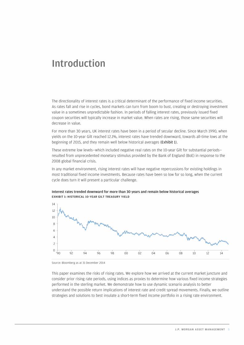
For more than 30 years, UK interest rates have been in a period of secular decline. Since March 1990, when yields on the 10-year Gilt reached 12.1%, interest rates have trended downward, towards all-time lows at the beginning of 2015, and they remain well below historical averages (Exhibit 1).

These extreme low levels—which included negative real rates on the 10-year Gilt for substantial periods—resulted from unprecedented monetary stimulus provided by the Bank of England (BoE) in response to the 2008 global financial crisis.

In any market environment, rising interest rates will have negative repercussions for existing holdings in most traditional fixed income investments. Because rates have been so low for so long, when the current cycle does turn it will present a particular challenge.

Interest rates trended downward for more than 30 years and remain below historical averagesEXHIBIT 1: HISTORICAL 10-YEAR GILT TREASURY YIELD

0

2

4

6

8

10

12

14

’90 92 94 96 98 00 02 04 06 08 10 12 14

Source: Bloomberg as at 31 December 2014

This paper examines the risks of rising rates. We explore how we arrived at the current market juncture and consider prior rising rate periods, using indices as proxies to determine how various fixed income strategies performed in the sterling market. We demonstrate how to use dynamic scenario analysis to better understand the possible return implications of interest rate and credit spread movements. Finally, we outline strategies and solutions to best insulate a short-term fixed income portfolio in a rising rate environment.

Introduction


The current era of low interest rates is best explained by the unprecedented actions that the BoE, the Federal Reserve (Fed) and other central banks have taken in response to the financial crisis. Quantitative easing (QE) by both the UK and US central banks involved extensive asset purchases in an effort to contain the crisis, limit its impact on the broader economy and aid the prolonged recovery by lowering longer-term interest rates to encourage investment and consumption.

The Fed and the BoE moved at a similar pace in their responses, and while the Fed had a zero-interest rate policy and QE in place by December 2008, the BoE reached a 0.5% low on the policy rate and launched its QE program shortly after, in March 2009. QE left both the US and UK central banks with elevated balance sheets. As of 31 December 2014, the BoE had over £400 billion on its balance sheet, versus approximately £100 billion in March 20081.

The first indication of a future rising rate cycle came in the spring of 2013, when Fed chairman Ben Bernanke signaled that the Fed could begin reducing its monthly asset purchases and investors began to fear earlier-than-expected rate tightening. Investors across global markets aggressively sold off both risk assets and Treasuries—the so-called “taper tantrum”. Ten-year Gilt yields rose from 1.7% in April 2013 to end the year at 3.03%.

At the start of 2014, many market participants projected that government bond yields would rise. Instead, yields fell, with the 10-year Gilt yielding 1.76% as of 31 December 2014. The unexpected declines reflected a variety of factors: continued stimulus and very low yields in many developed markets, persistent demand for risk-free assets and growing concern about the fading strength of the global economy.

When it does decide to act, we expect that the BoE will move gradually to raise rates, amid muted inflation pressures and expectations, lingering labour market slack and ongoing concern about derailing economic growth. Unlike the Fed in the US, the BoE has committed to raising interest rates before reducing its Asset Purchasing Programme. The BoE also projects that rates will peak at lower levels than they have in the past. UK officials have said that rate hikes will be more “gradual and limited”2 and that the official policy rate is likely to settle at a lower level, somewhere in the region of 2.5% or 3%, rather than the longer-term average of 5%. In the eurozone, on the other hand, rates will likely remain low for an extended period, as the European Central Bank (ECB) tackles deflationary pressures with negative deposit rates, QE and a wide range of extraordinary stimulus measures.

Extraordinary response to an extraordinary crisis

1 Source: http://www.bankofengland.co.uk/markets/Pages/balancesheet/default.aspx2 Source: http://www.bankofengland.co.uk/publications/Documents/inflationreport/2014/irspnote140212.pdf

http://www.bankofengland.co.uk/markets/Pages/balancesheet/default.aspx

http://www.bankofengland.co.uk/publications/Documents/inflationreport/2014/irspnote140212.pdf


Investors anticipating rising rates would be well served to include as part of their strategic decision-making process a review of the five major periods of UK monetary tightening and rising interest rates that occurred over the last 20 years:

Period 1 December 1993 to February 1995

Period 2 October 1996 to November 1997

Period 3 April 1999 to February 2000

Period 4 March 2003 to August 2004

Period 5 July 2005 to July 2007

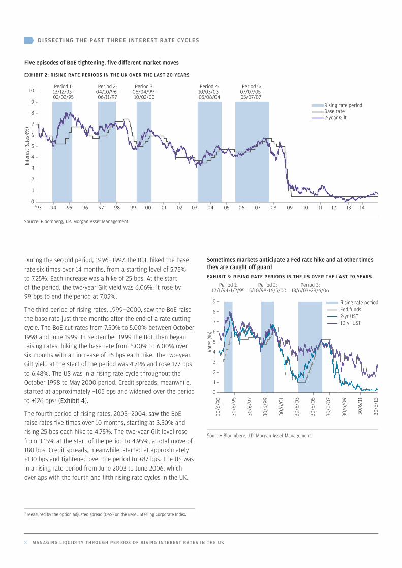
In the following pages we consider the performance of different short duration fixed income strategies. We include an analysis of credit spread movement for the third, fourth and fifth hiking cycles: data for the first and second cycles is not available. Each period saw increasing BoE base rates as well as rising Gilt yields.1 In most periods the markets were able to anticipate and price in the tightening of monetary policy before the base rate moved. This is evidenced in the rise of Gilt yields roughly eight to 12 months prior to monetary policy tightening in each respective period. But the 1997 tightening caught markets off guard. Both the base rate and Gilt yields began to move higher at roughly the same time (Exhibit 2).

The precise start and end points of a rising rate period are open to debate. We define the start of the period as the point at which two-year Gilt yields begin to rise. The period ends when the BoE stops increasing the base rate.

A rising rate period can be characterised by its starting conditions and the pace at which rates rise. During the 1993—1995 period (Period 1), the BoE hiked the base rate three times over six months, from 5.25% to 6.75%. The BoE hiked by 50 basis points (bps) each time it increased the base rate. At the start of the period, the two-year Gilt yield was 4.96% and rose by 287 bps to end at 7.83%. This rising rate period occurred at a similar time to a rising rate period in the US (Exhibit 3).

Dissecting the past three interest rate cycles

1 The Bank of England assumed operational responsibility to set interest rates independently from June 1997 and this was enshrined in law in the Back of England Act 1998. Prior to this rates were set by Her Majesty’s Treasury.

DISSECTING THE PAST THREE INTEREST RATE CYCLES


Five episodes of BoE tightening, five different market moves

EXHIBIT 2: RISING RATE PERIODS IN THE UK OVER THE LAST 20 YEARS

0

1

2

3

4

5

6

7

8

9

10

’93 94 95 96 97 98 99 00 01 02 05 09 1203 04 06 07 08 10 11 13 14

Rising rate period Base rate 2-year Gilt

Period 1:13/12/93–02/02/95

Inte

rest

Rat

es (%

)

Period 2:04/10/96–06/11/97

Period 3:06/04/99–10/02/00

Period 4:10/03/03–05/08/04

Period 5:07/07/05–05/07/07

Source: Bloomberg, J.P. Morgan Asset Management.

During the second period, 1996—1997, the BoE hiked the base rate six times over 14 months, from a starting level of 5.75% to 7.25%. Each increase was a hike of 25 bps. At the start of the period, the two-year Gilt yield was 6.06%. It rose by 99 bps to end the period at 7.05%.

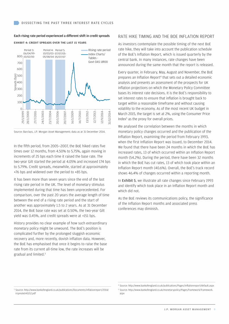
The third period of rising rates, 1999—2000, saw the BoE raise the base rate just three months after the end of a rate cutting cycle. The BoE cut rates from 7.50% to 5.00% between October 1998 and June 1999. In September 1999 the BoE then began raising rates, hiking the base rate from 5.00% to 6.00% over six months with an increase of 25 bps each hike. The two-year Gilt yield at the start of the period was 4.71% and rose 177 bps to 6.48%. The US was in a rising rate cycle throughout the October 1998 to May 2000 period. Credit spreads, meanwhile, started at approximately +105 bps and widened over the period to +126 bps2 (Exhibit 4).

The fourth period of rising rates, 2003—2004, saw the BoE raise rates five times over 10 months, starting at 3.50% and rising 25 bps each hike to 4.75%. The two-year Gilt level rose from 3.15% at the start of the period to 4.95%, a total move of 180 bps. Credit spreads, meanwhile, started at approximately +130 bps and tightened over the period to +87 bps. The US was in a rising rate period from June 2003 to June 2006, which overlaps with the fourth and fifth rising rate cycles in the UK.

Sometimes markets anticipate a Fed rate hike and at other times they are caught off guardEXHIBIT 3: RISING RATE PERIODS IN THE US OVER THE LAST 20 YEARS

Fed funds2-yr UST10-yr UST

0

1

2

3

4

5

6

9

8

7

30/6

/93

30/6

/95

30/6

/97

30/6

/99

30/6

/01

30/6

/03

30/6

/05

30/0

/07

30/6

/09

30/6

/11

30/6

/13

Rate

s (%

)

Period 1:12/1/94–1/2/95

Period 2:5/10/98–16/5/00

Period 3:13/6/03–29/6/06

Rising rate period


2 Measured by the option adjusted spread (OAS) on the BAML Sterling Corporate Index.



Each rising rate period experienced a different shift in credit spreads

EXHIBIT 4: CREDIT SPREADS OVER THE LAST 15 YEARS

31/1

2/20

14

12/9

/201

4

12/7

/201

3

13/1

/201

2

16/7

/201

0

16/1

/200

9

20

/7/2

007

20/1

/200

6

23/7

/200

4

24/1

/200

3

27/7

/200

1

28/1

/200

0

29/1

/199

9

Period 3: 06/04/99-10/02/00

Period 4: 10/03/03-05/08/04

Period 5: 07/07/05-05/07/07

Rising rate period Index Charts/Tables - Govt OAS UR00

0

100

Spre

ads

(bps

)

200

300

400

500

600

700

800

Source: Barclays, J.P. Morgan Asset Management; data as at 31 December 2014.

In the fifth period, from 2005—2007, the BoE hiked rates five times over 12 months, from 4.50% to 5.75%, again moving in increments of 25 bps each time it raised the base rate. The two-year Gilt started the period at 4.05% and increased 174 bps to 5.79%. Credit spreads, meanwhile, started at approximately +76 bps and widened over the period to +85 bps.

It has been more than seven years since the end of the last rising rate period in the UK. The level of monetary stimulus implemented during that time has been unprecedented. For comparison, over the past 20 years the average length of time between the end of a rising rate period and the start of another was approximately 1.5 to 2 years. As at 31 December 2014, the BoE base rate was set at 0.50%, the two-year Gilt yield was 0.45%, and credit spreads were at +151 bps.

History provides no clear example of how such extraordinary monetary policy might be unwound. The BoE’s position is complicated further by the prolonged sluggish economic recovery and, more recently, dovish inflation data. However, the BoE has emphasised that once it begins to raise the base rate from its current all-time low, the rate increases will be gradual and limited.3

RATE HIKE TIMING AND THE BOE INFLATION REPORT

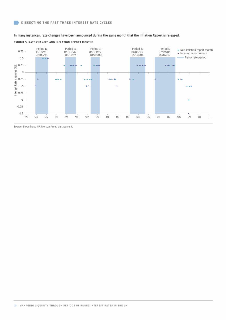
As investors contemplate the possible timing of the next BoE rate hike, they will take into account the publication schedule of the BoE’s Inflation Report, which is issued quarterly by the central bank. In many instances, rate changes have been announced during the same month that the report is released.

Every quarter, in February, May, August and November, the BoE prepares an Inflation Report4 that sets out a detailed economic analysis and presents an assessment of the prospects for UK inflation projections on which the Monetary Policy Committee bases its interest rate decisions. It is the BoE’s responsibility to set interest rates to ensure that inflation is brought back to target within a reasonable timeframe and without causing volatility to the economy. As of the most recent UK budget in March 2015, the target is set at 2%, using the Consumer Price Index5 as the proxy for overall prices.

We analysed the correlation between the months in which monetary policy changes occurred and the publication of the Inflation Report, examining the period from February 1993, when the first Inflation Report was issued, to December 2014. We found that there have been 24 months in which the BoE has increased rates, 13 of which occurred within an Inflation Report month (54.2%). During the period, there have been 32 months in which the BoE has cut rates, 13 of which took place within an Inflation Report month (40.6%). Overall, the BoE’s track record shows 46.4% of changes occurred within a reporting month.

In Exhibit 5, we illustrate all rate changes since February 1993 and identify which took place in an Inflation Report month and which did not.

As the BoE reviews its communications policy, the significance of the Inflation Report months and associated press conferences may diminish.

3 Source: http://www.bankofengland.co.uk/publications/Documents/inflationreport/2014/irspnote140212.pdf

4 Source: http://www.bankofengland.co.uk/publications/Pages/inflationreport/default.aspx5 Source: http://www.bankofengland.co.uk/monetarypolicy/Pages/framework/framework.

aspx



http://www.bankofengland.co.uk/publications/Pages/inflationreport/default.aspx

http://www.bankofengland.co.uk/monetarypolicy/Pages/framework/framework.aspx

http://www.bankofengland.co.uk/monetarypolicy/Pages/framework/framework.aspx



In many instances, rate changes have been announced during the same month that the Inflation Report is released.

EXHIBIT 5: RATE CHANGES AND INFLATION REPORT MONTHS

-1.5

-1.25

-1

-0.75

-0.5

-0.25

0

0.25

0.5

0.75

’93 95 97 99 01 03 05 07 09 94 96 98 00 02 04 06 08 10 11

Non-inflation report monthInflation report month

Period 1:13/12/93–02/02/95

Period 2:04/10/96–06/11/97

Period 3:06/04/99–10/02/00

Period 4:10/03/03–05/08/04

Period 5:07/07/05–05/07/07

Rising rate period

Inte

rest

Rat

e ch

ange

s (%

)



SHORTER DURATION STRATEGIES OUTPERFORMED

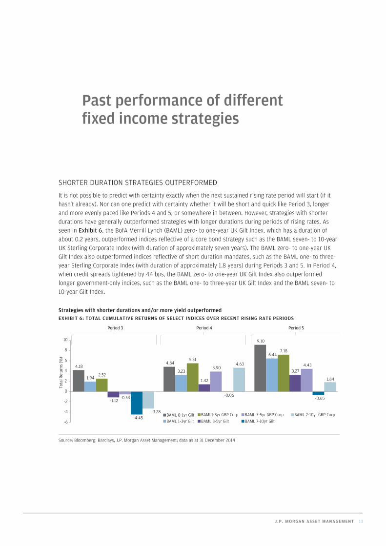
It is not possible to predict with certainty exactly when the next sustained rising rate period will start (if it hasn’t already). Nor can one predict with certainty whether it will be short and quick like Period 3, longer and more evenly paced like Periods 4 and 5, or somewhere in between. However, strategies with shorter durations have generally outperformed strategies with longer durations during periods of rising rates. As seen in Exhibit 6, the BofA Merrill Lynch (BAML) zero- to one-year UK Gilt Index, which has a duration of about 0.2 years, outperformed indices reflective of a core bond strategy such as the BAML seven- to 10-year UK Sterling Corporate Index (with duration of approximately seven years). The BAML zero- to one-year UK Gilt Index also outperformed indices reflective of short duration mandates, such as the BAML one- to three-year Sterling Corporate Index (with duration of approximately 1.8 years) during Periods 3 and 5. In Period 4, when credit spreads tightened by 44 bps, the BAML zero- to one-year UK Gilt Index also outperformed longer government-only indices, such as the BAML one- to three-year UK Gilt Index and the BAML seven- to 10-year Gilt Index.

Strategies with shorter durations and/or more yield outperformedEXHIBIT 6: TOTAL CUMULATIVE RETURNS OF SELECT INDICES OVER RECENT RISING RATE PERIODS

4.18

1.94 2.52

-1.12 -0.53

-4.45 -3.28

4.84

3.23

5.51

1.42

3.90

-0.06

4.63

9.10

6.44 7.18

3.27 4.43

-0.65

1.84

-6

-4

-2

0

2

4

6

8

10

Tota

l Ret

urns

(%)

BAML 0-1yr Gilt BAML 1-3yr Gilt

BAML1-3yr GBP Corp BAML 3-5yr Gilt

BAML 3-5yr GBP Corp BAML 7-10yr Gilt

BAML 7-10yr GBP Corp

Period 3 Period 4 Period 5

Source: Bloomberg, Barclays, J.P. Morgan Asset Management; data as at 31 December 2014

Past performance of different fixed income strategies


PAST PERFORMANCE OF DIFFERENT FIXED INCOME STRATEGIES

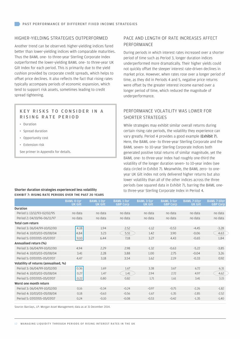
HIGHER-YIELDING STRATEGIES OUTPERFORMED

Another trend can be observed: higher-yielding indices fared better than lower-yielding indices with comparable maturities. Thus the BAML one- to three-year Sterling Corporate Index outperformed the lower-yielding BAML one- to three-year UK Gilt Index for each period. This is primarily due to the yield cushion provided by corporate credit spreads, which helps to offset price declines. It also reflects the fact that rising rates typically accompany periods of economic expansion, which tend to support risk assets, sometimes leading to credit spread tightening.

K E Y R I S K S T O C O N S I D E R I N A R I S I N G R A T E P E R I O D• Duration

• Spread duration

• Opportunity cost

• Extension risk

See primer in Appendix for details.

PACE AND LENGTH OF RATE INCREASES AFFECT PERFORMANCE

During periods in which interest rates increased over a shorter period of time such as Period 3, longer duration indices underperformed more dramatically. Their higher yields could not quickly offset the steeper interest rate-driven declines in market price. However, when rates rose over a longer period of time, as they did in Periods 4 and 5, negative price returns were offset by the greater interest income earned over a longer period of time, which reduced the magnitude of underperformance.

PERFORMANCE VOLATILITY WAS LOWER FOR SHORTER STRATEGIES

While strategies may exhibit similar overall returns during certain rising rate periods, the volatility they experience can vary greatly. Period 4 provides a good example (Exhibit 7). Here, the BAML one- to three-year Sterling Corporate and the BAML seven- to 10-year Sterling Corporate Indices both generated positive total returns of similar magnitude, yet the BAML one- to three-year Index had roughly one-third the volatility of the longer duration seven- to 10-year index (see data circled in Exhibit 7). Meanwhile, the BAML zero- to one-year UK Gilt index not only delivered higher returns but also lower volatility than all of the other indices across the three periods (see squared data in Exhibit 7), barring the BAML one- to three-year Sterling Corporate Index in Period 4. Shorter duration strategies experienced less volatility

EXHIBIT 7: RISING RATE PERIODS OVER THE PAST 20 YEARS

BAML 0-1yr UK Gilt

BAML 1-3yr UK Gilt

BAML 1-3yr GBP Corp

BAML 3-5yr UK Gilt

BAML 3-5yr GBP Corp

BAML 7-10yr UK Gilt

BAML 7-10yr GBP Corp

DurationPeriod 1: 13/12/93–02/02/95 no data no data no data no data no data no data no dataPeriod 2: 04/10/96–06/11/97 no data no data no data no data no data no data no data

Total cum returnPeriod 3: 06/04/99–10/02/00 4.18 1.94 2.52 -1.12 -0.53 -4.45 -3.28Period 4: 10/03/03–05/08/04 4.84 3.23 5.51 1.42 3.90 -0.06 4.63Period 5: 07/07/05–05/07/07 9.10 6.44 7.18 3.27 4.43 -0.65 1.84

Annualised return (%)Period 3: 06/04/99–10/02/00 4.94 2.29 2.98 -1.32 -0.63 -5.22 -3.85Period 4: 10/03/03–05/08/04 3.41 2.28 3.88 1.00 2.75 -0.04 3.26Period 5: 07/07/05–05/07/07 4.47 3.18 3.54 1.62 2.19 -0.33 0.92

Volatility of returns (annualised, %)Period 3: 06/04/99–10/02/00 0.36 1.69 1.67 3.38 3.67 6.72 6.31

Period 4: 10/03/03–05/08/04 0.27 1.47 1.41 2.94 2.72 4.97 4.62

Period 5: 07/07/05–05/07/07 0.22 0.80 0.82 1.71 1.61 3.41 3.15

Worst one month returnPeriod 3: 06/04/99–10/02/00 0.16 -0.34 -0.24 -0.97 -0.75 -2.26 -1.82

Period 4: 10/03/03–05/08/04 0.18 -0.63 -0.56 -1.67 -1.35 -2.85 -2.52

Period 5: 07/07/05–05/07/07 0.24 -0.10 -0.08 -0.53 -0.42 -1.35 -1.40



As we have seen, in a rising rate period a portfolio invested in longer tenor fixed coupon bonds will likely suffer lower total returns than one invested in shorter tenor fixed coupon bonds. Beyond that basic principle, it is worth remembering that there are two components of total return—price and income—which we can analyse using sensitivity analysis.

In this paper, a sensitivity analysis begins by looking at the UK Treasury yield (UKT) curve as at 31 December 2014, using tenors in six-month increments out to three years. We then “shock,” or change, the yield at each point along the curve, resulting in a hypothetical yield curve for six months into the future. Using this hypothetical shift in the curve, we estimate the approximate six-month total return for the period commencing 31 December 2014. We then separate this total return into its income and price components. We analyse four different scenarios here for illustrative purposes.

Using sensitivity analysis to prepare for rising rates


USING SENSITIVITY ANALYSIS TO PREPARE FOR RISING RATES

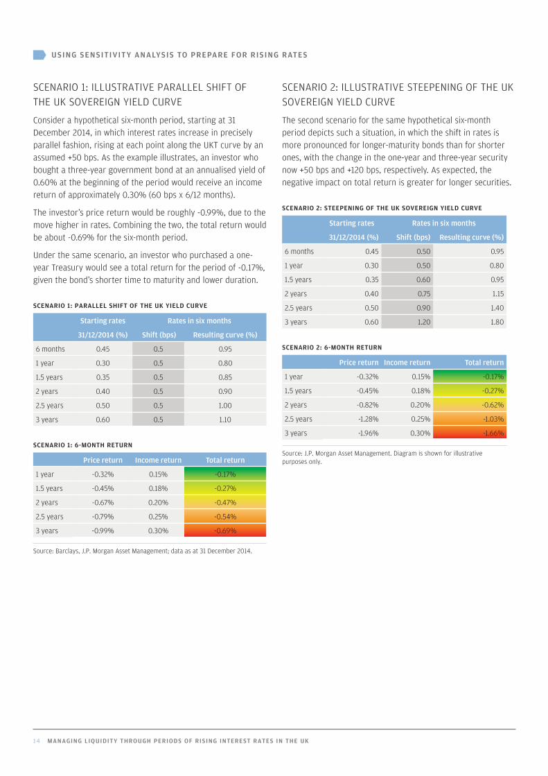
SCENARIO 1: ILLUSTRATIVE PARALLEL SHIFT OF THE UK SOVEREIGN YIELD CURVE

Consider a hypothetical six-month period, starting at 31 December 2014, in which interest rates increase in precisely parallel fashion, rising at each point along the UKT curve by an assumed +50 bps. As the example illustrates, an investor who bought a three-year government bond at an annualised yield of 0.60% at the beginning of the period would receive an income return of approximately 0.30% (60 bps x 6/12 months).

The investor’s price return would be roughly -0.99%, due to the move higher in rates. Combining the two, the total return would be about -0.69% for the six-month period.

Under the same scenario, an investor who purchased a one-year Treasury would see a total return for the period of -0.17%, given the bond’s shorter time to maturity and lower duration.

SCENARIO 1: PARALLEL SHIFT OF THE UK YIELD CURVE

Starting rates Rates in six months

31/12/2014 (%) Shift (bps) Resulting curve (%)

6 months 0.45 0.5 0.95

1 year 0.30 0.5 0.80

1.5 years 0.35 0.5 0.85

2 years 0.40 0.5 0.90

2.5 years 0.50 0.5 1.00

3 years 0.60 0.5 1.10

SCENARIO 1: 6-MONTH RETURN

Price return Income return Total return

1 year -0.32% 0.15% -0.17%

1.5 years -0.45% 0.18% -0.27%

2 years -0.67% 0.20% -0.47%

2.5 years -0.79% 0.25% -0.54%

3 years -0.99% 0.30% -0.69%


SCENARIO 2: ILLUSTRATIVE STEEPENING OF THE UK SOVEREIGN YIELD CURVE

The second scenario for the same hypothetical six-month period depicts such a situation, in which the shift in rates is more pronounced for longer-maturity bonds than for shorter ones, with the change in the one-year and three-year security now +50 bps and +120 bps, respectively. As expected, the negative impact on total return is greater for longer securities.

SCENARIO 2: STEEPENING OF THE UK SOVEREIGN YIELD CURVE

Starting rates Rates in six months

31/12/2014 (%) Shift (bps) Resulting curve (%)

6 months 0.45 0.50 0.95

1 year 0.30 0.50 0.80

1.5 years 0.35 0.60 0.95

2 years 0.40 0.75 1.15

2.5 years 0.50 0.90 1.40

3 years 0.60 1.20 1.80



1 year -0.32% 0.15% -0.17%

1.5 years -0.45% 0.18% -0.27%

2 years -0.82% 0.20% -0.62%

2.5 years -1.28% 0.25% -1.03%

3 years -1.96% 0.30% -1.66%

Source: J.P. Morgan Asset Management. Diagram is shown for illustrative purposes only.


USING SENSITIVITY ANALYSIS TO PREPARE FOR RISING RATES

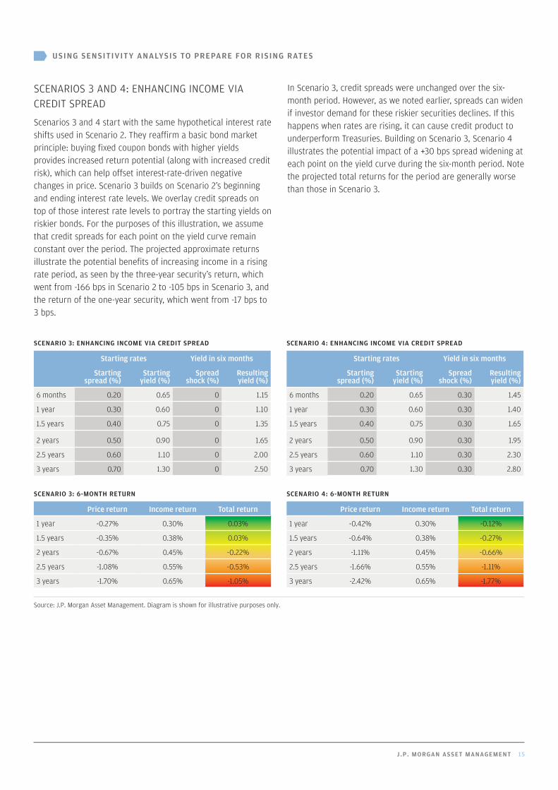
SCENARIOS 3 AND 4: ENHANCING INCOME VIA CREDIT SPREAD

Scenarios 3 and 4 start with the same hypothetical interest rate shifts used in Scenario 2. They reaffirm a basic bond market principle: buying fixed coupon bonds with higher yields provides increased return potential (along with increased credit risk), which can help offset interest-rate-driven negative changes in price. Scenario 3 builds on Scenario 2’s beginning and ending interest rate levels. We overlay credit spreads on top of those interest rate levels to portray the starting yields on riskier bonds. For the purposes of this illustration, we assume that credit spreads for each point on the yield curve remain constant over the period. The projected approximate returns illustrate the potential benefits of increasing income in a rising rate period, as seen by the three-year security’s return, which went from -166 bps in Scenario 2 to -105 bps in Scenario 3, and the return of the one-year security, which went from -17 bps to 3 bps.

In Scenario 3, credit spreads were unchanged over the six- month period. However, as we noted earlier, spreads can widen if investor demand for these riskier securities declines. If this happens when rates are rising, it can cause credit product to underperform Treasuries. Building on Scenario 3, Scenario 4 illustrates the potential impact of a +30 bps spread widening at each point on the yield curve during the six-month period. Note the projected total returns for the period are generally worse than those in Scenario 3.

SCENARIO 3: ENHANCING INCOME VIA CREDIT SPREAD

Starting rates Yield in six months

Starting spread (%)

Starting yield (%)

Spread shock (%)

Resulting yield (%)

6 months 0.20 0.65 0 1.15

1 year 0.30 0.60 0 1.10

1.5 years 0.40 0.75 0 1.35

2 years 0.50 0.90 0 1.65

2.5 years 0.60 1.10 0 2.00

3 years 0.70 1.30 0 2.50



1 year -0.27% 0.30% 0.03%

1.5 years -0.35% 0.38% 0.03%

2 years -0.67% 0.45% -0.22%

2.5 years -1.08% 0.55% -0.53%

3 years -1.70% 0.65% -1.05%

SCENARIO 4: ENHANCING INCOME VIA CREDIT SPREAD

Starting rates Yield in six months

Starting spread (%)

Starting yield (%)

Spread shock (%)

Resulting yield (%)

6 months 0.20 0.65 0.30 1.45

1 year 0.30 0.60 0.30 1.40

1.5 years 0.40 0.75 0.30 1.65

2 years 0.50 0.90 0.30 1.95

2.5 years 0.60 1.10 0.30 2.30

3 years 0.70 1.30 0.30 2.80



1 year -0.42% 0.30% -0.12%

1.5 years -0.64% 0.38% -0.27%

2 years -1.11% 0.45% -0.66%

2.5 years -1.66% 0.55% -1.11%

3 years -2.42% 0.65% -1.77%

Source: J.P. Morgan Asset Management. Diagram is shown for illustrative purposes only.


How can an investor protect a portfolio of bonds in a period of rising rates? Though some investors may choose to simply exit the asset class, there are strong arguments for maintaining a core allocation to fixed income. In most interest rate environments, fixed income provides diversification, a steady stream of income and a lower volatility investment over time. Additionally, fixed income portfolios with longer durations have provided higher returns, albeit with greater volatility, over longer time horizons.

However, for investors with shorter investment horizons (especially those with potential near term cash needs) or those seeking to protect profits realised from longer duration strategies, mitigating potential volatility during the anticipated rising rate environment is a key priority. To that end, investors should consider how they can best employ two effective strategies for managing a rising rate environment: shortening duration and increasing income.

SHORTENING A PORTFOLIO’S WEIGHTED AVERAGE DURATION

The most effective way to protect a portfolio from the impact of rising rates is to reduce its weighted average duration. In traditional fixed income portfolios, this is typically achieved using one or more of the following methods:

• Sales of longer-dated fixed coupon securities and/or reinvestment of interest income and cash from matured securities into those with shorter tenors.

• Purchases of floating rate notes, whose coupons reset on a regular basis. As a floater’s coupon resets to adjust for market changes, leading to lower duration, its price should typically experience less volatility.1

• Investments in higher-coupon or higher-yielding securities, which have shorter interest rate durations relative to lower-yielding bonds with the same maturity.

Strategies for insulating a fixed income portfolio

1 Most floating rate notes reset interest rates on a monthly or quarterly basis. Thus durations on these securities are typically shorter than three months. However, it is important to note that while the owners of such bonds have limited exposure to changes in interest rates, they are exposed to the creditworthiness of the borrower until the final maturity of the bond. This means that floating rate bonds not issued by the UK government can have longer spread durations than interest rate durations. This can result in greater volatility should credit conditions change.


STRATEGIES FOR INSULATING A FIXED INCOME PORTFOLIO

INCREASING THE INTEREST INCOME COMPONENT OF TOTAL RETURN

Increased income or yield not only lowers duration but also provides greater income return, helping to offset declines in price during periods of rising rates. However, higher yields due to increased credit exposure come with added risk. If credit spreads widen in conjunction with rising rates, these securities could underperform, as seen in Scenario 4 of our sensitivity analysis. In addition to interest rate duration, fixed income investors must also be cognisant of spread duration. Bonds with longer spread durations will typically be more negatively impacted by widening credit spreads than bonds with shorter spread durations.

As seen in prior periods of rising rates, credit spreads may tighten, widen or even remain flat. When rates start to rise, it is important for investors to understand not only where credit spreads are but also where starting yields are relative to historical levels. The extremely low levels on risk-free rates over the last few years have forced investors to seek yield in riskier securities, resulting in tighter credit spreads and low absolute yields. As at 31 December 2014, the credit spread of the BoA Merrill Lynch Stanley Cap Index was at 151 bps, down from extreme highs in March 2009 of about 700 bps and below its 10-year average of 214 bps. It is possible that, as investors sell fixed income securities in anticipation of higher rates, sales will not be limited to risk-free Treasuries alone and credit product may see spreads widen.

S H O R T D U R A T I O N I N V E S T M E N T S T R A T E G I E SWhen considering the key elements of investing in a rising rate environment—duration, income, credit spread exposure—investors can choose among a variety of traditional short-term fixed income products:

1. A series of overnight deposits These will have negligible duration. Generally, they closely track movements in short-term rates and will likely perform best if rates rise sharply over a short period of time. Direct investments with a small number of banks will reduce diversification benefits and should be done in conjunction with in-depth credit analysis. Returns over longer periods may be lower than those on more diversified investment options.

2. Term deposits Durations range from zero to one year. Term deposits are not marked-to-market, which means there are no unrealised losses. The instruments are not liquid, as there is no secondary market and the buyer typically agrees to withdraw principal only at the end of the stated term. Additionally, when rates are rising, the income received at maturity will generally be lower than that from a series of shorter deposits, as the investor is locked into the lower rate for longer.

3. Money market portfolios These typically have weighted average maturities of less than 60 days. Fund yields will rise in line with prevailing interest rates on a lagged basis depending on the fund’s weighted average maturity. These investments seek to eliminate principal losses through their stable net asset value (NAV).

4. Managed reserves This is J.P. Morgan’s definition of the segment between money market and short duration bond funds. Funds in this category seek to generate higher total returns than money market funds while focusing on principal preservation and segmented liquidity needs. They typically have durations between three months and one year, have short-term benchmarks (BAML Index) and exhibit lower

performance volatility than short-term bond funds. Due to their slightly longer durations (relative to money market funds) and mark-to-market accounting, unrealised losses can occur when rates rise, causing negative returns. However, because of the structure of these portfolios and their short duration, negative returns should be relatively short-lived. Historically, these funds have outperformed money market funds over longer time horizons.

5. Short-term bond funds These funds usually have durations between one and three years and will generally have higher yields than managed reserves funds. They are typically benchmarked against indices such as the BAML one- to three-year UK Gilt Index. Due to their longer durations, unrealised losses are likely when rates rise. Short-term bond funds have traditionally outperformed managed reserves funds over longer time periods, albeit with greater volatility.

6. Custom strategies These strategies are designed to meet the specific objectives and risk tolerances of a given investor and can be implemented for any of the product types, or combinations of product types, described above.

7. Active management Money market portfolios, managed reserves and short duration funds are typically actively managed strategies. Active management allows investment professionals to best navigate the uncertainty and volatility caused by the specter of rising rates. They can take advantage of market opportunities by managing duration, sector rotation and security selection.


More than seven years have passed since the end of the last period of rising rates. Unprecedented actions by the BoE have left interest rates well below historical averages. As key economic metrics improve, indications are that the BoE will first look to increase interest rates and then look to end expansionary monetary policy.

While past precedents can provide some clues as to the possible paths a rise in rates will take, it is impossible to predict with certainty what the unwinding of such extraordinary monetary stimulus may look like. The only certainty is that when rates do rise, market values of portfolios of existing fixed coupon bonds will be negatively affected.

To prepare, investors are well advised to develop a thorough understanding of past market behaviour. Their strategic decision-making process should also be guided by a robust scenario analysis of the future possible directions of interest rates, credit spreads and the shape of the yield curve. Finally, it is essential that the evaluation of various investment strategies be informed by the investor’s short-term cash needs and risk tolerance.

As this paper has demonstrated, using historical analysis and illustrative sensitivity scenarios, investors who seek liquid portfolios with limited exposure to the negative impacts of rising rates should find an effective solution in shorter duration, higher income strategies.

Conclusion: Historical knowledge, dynamic insight


BOND RETURNS

There are two primary components of a bond’s total return for a given period: interest income and change in price. Interest income return is driven by the coupon the bond pays or accrues over the period, while price return is based on the change in market price. A bond’s market price fluctuates due to changes in the yield demanded by investors as well as any accretion (or amortisation) of bonds that trade at a discount (or premium), which is due to the “pull to par” effect. Both of these factors will be discussed in more detail in the following sections.

BOND VALUATION

A bond’s price is equal to the present value of its future cash flows discounted at a given interest rate or set of rates. As the required yields demanded by investors increase (or decrease), the discount factor(s) applied to those cash flows increase (or decrease) and the present value, or price, of the bond falls (or rises). This explains the inverse relationship between interest rate movements and the change in prices on existing fixed coupon bonds.

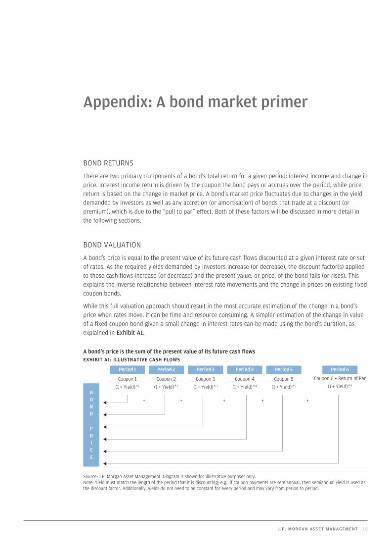
While this full valuation approach should result in the most accurate estimation of the change in a bond’s price when rates move, it can be time and resource consuming. A simpler estimation of the change in value of a fixed coupon bond given a small change in interest rates can be made using the bond’s duration, as explained in Exhibit A1.

A bond’s price is the sum of the present value of its future cash flowsEXHIBIT A1: ILLUSTRATIVE CASH FLOWS

BOND

PRICE

Coupon 1

(1 + Yield)^1

Period 1

Coupon 2

(1 + Yield)^2

Period 2

Coupon 3

(1 + Yield)^3

Period 3

Coupon 4

(1 + Yield)^4

Period 4

Coupon 5

(1 + Yield)^5

Period 5

Coupon 6 + Return of Par

(1 + Yield)^6

Period 6

+ + + + +

Source: J.P. Morgan Asset Management. Diagram is shown for illustrative purposes only. Note: Yield must match the length of the period that it is discounting; e.g., if coupon payments are semiannual, then semiannual yield is used as the discount factor. Additionally, yields do not need to be constant for every period and may vary from period to period.

Appendix: A bond market primer


APPENDIX: A BOND MARKET PRIMER

DURATION

Generally speaking, the duration of a bond is an estimate of the sensitivity of its price to a change in interest rates, also referred to as interest rate duration. The larger (i.e., longer) the duration, which is stated in years, the more sensitive a bond’s price is. For example, if a fixed coupon bond’s duration is two years and interest rates increase by 50 bps (0.50%), the duration would estimate an approximate 1% drop in its price (2 x 0.005). Assuming it was initially priced at par ($100), then the new price would be approximately $99. For a bond with a five-year duration, the expected price decrease would be approximately -2.5%, to $97.50. The duration of a portfolio of bonds is the market-weighted average of the duration of all the holdings in that portfolio.

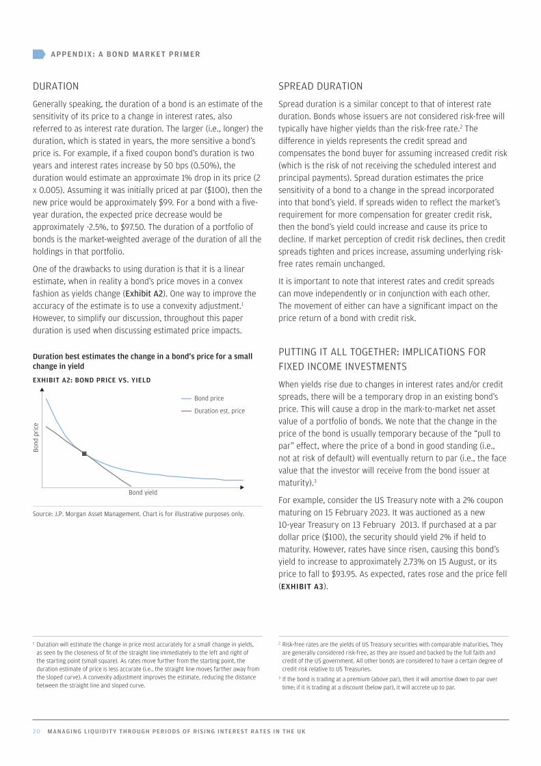
One of the drawbacks to using duration is that it is a linear estimate, when in reality a bond’s price moves in a convex fashion as yields change (Exhibit A2). One way to improve the accuracy of the estimate is to use a convexity adjustment.1 However, to simplify our discussion, throughout this paper duration is used when discussing estimated price impacts.

Duration best estimates the change in a bond’s price for a small change in yield

EXHIBIT A2: BOND PRICE VS. YIELD

Bond

pric

e

Bond yield

Bond price

Duration est. price

Source: J.P. Morgan Asset Management. Chart is for illustrative purposes only.

SPREAD DURATION

Spread duration is a similar concept to that of interest rate duration. Bonds whose issuers are not considered risk-free will typically have higher yields than the risk-free rate.2 The difference in yields represents the credit spread and compensates the bond buyer for assuming increased credit risk (which is the risk of not receiving the scheduled interest and principal payments). Spread duration estimates the price sensitivity of a bond to a change in the spread incorporated into that bond’s yield. If spreads widen to reflect the market’s requirement for more compensation for greater credit risk, then the bond’s yield could increase and cause its price to decline. If market perception of credit risk declines, then credit spreads tighten and prices increase, assuming underlying risk-free rates remain unchanged.

It is important to note that interest rates and credit spreads can move independently or in conjunction with each other. The movement of either can have a significant impact on the price return of a bond with credit risk.

PUTTING IT ALL TOGETHER: IMPLICATIONS FOR FIXED INCOME INVESTMENTS

When yields rise due to changes in interest rates and/or credit spreads, there will be a temporary drop in an existing bond’s price. This will cause a drop in the mark-to-market net asset value of a portfolio of bonds. We note that the change in the price of the bond is usually temporary because of the “pull to par” effect, where the price of a bond in good standing (i.e., not at risk of default) will eventually return to par (i.e., the face value that the investor will receive from the bond issuer at maturity).3

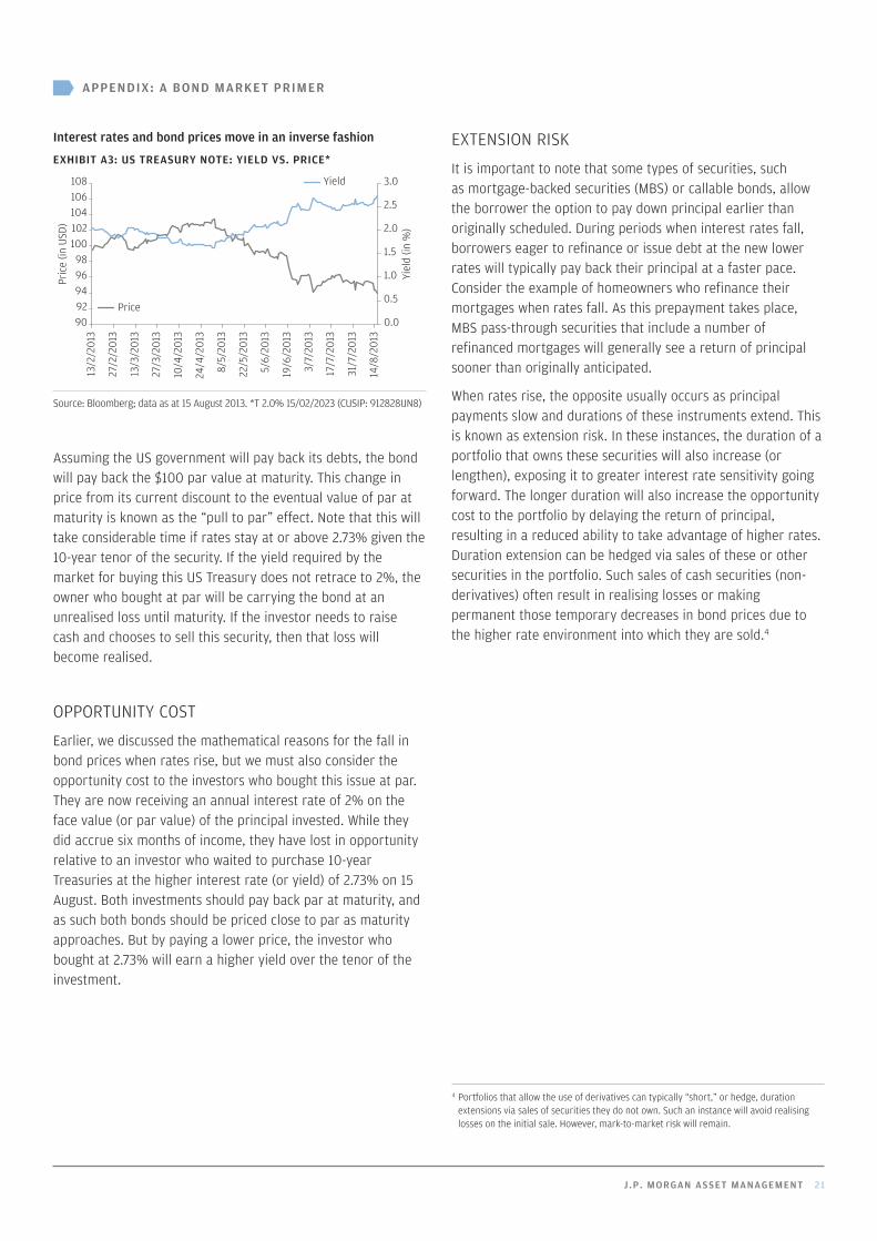
For example, consider the US Treasury note with a 2% coupon maturing on 15 February 2023. It was auctioned as a new 10-year Treasury on 13 February 2013. If purchased at a par dollar price ($100), the security should yield 2% if held to maturity. However, rates have since risen, causing this bond’s yield to increase to approximately 2.73% on 15 August, or its price to fall to $93.95. As expected, rates rose and the price fell (EXHIBIT A3).

1 Duration will estimate the change in price most accurately for a small change in yields, as seen by the closeness of fit of the straight line immediately to the left and right of the starting point (small square). As rates move further from the starting point, the duration estimate of price is less accurate (i.e., the straight line moves farther away from the sloped curve). A convexity adjustment improves the estimate, reducing the distance between the straight line and sloped curve.

2 Risk-free rates are the yields of US Treasury securities with comparable maturities. They are generally considered risk-free, as they are issued and backed by the full faith and credit of the US government. All other bonds are considered to have a certain degree of credit risk relative to US Treasuries.

3 If the bond is trading at a premium (above par), then it will amortise down to par over time; if it is trading at a discount (below par), it will accrete up to par.


APPENDIX: A BOND MARKET PRIMER

Interest rates and bond prices move in an inverse fashion

EXHIBIT A3: US TREASURY NOTE: YIELD VS. PRICE*

Yiel

d (in

%)

Pric

e (in

USD

)

Price

Yield

0.0

0.5

1.0

1.5

2.0

2.5

3.0

9092949698

100102104106108

13/2

/201

3

27/2

/201

3

13/3

/201

3

27/3

/201

3

10/4

/201

3

24/4

/201

3

8/5/

2013

22/5

/201

3

5/6/

2013

19/6

/201

3

3/7/

2013

17/7

/201

3

31/7

/201

3

14/8

/201

3

Source: Bloomberg; data as at 15 August 2013. *T 2.0% 15/02/2023 (CUSIP: 912828UN8)

Assuming the US government will pay back its debts, the bond will pay back the $100 par value at maturity. This change in price from its current discount to the eventual value of par at maturity is known as the “pull to par” effect. Note that this will take considerable time if rates stay at or above 2.73% given the 10-year tenor of the security. If the yield required by the market for buying this US Treasury does not retrace to 2%, the owner who bought at par will be carrying the bond at an unrealised loss until maturity. If the investor needs to raise cash and chooses to sell this security, then that loss will become realised.

OPPORTUNITY COST

Earlier, we discussed the mathematical reasons for the fall in bond prices when rates rise, but we must also consider the opportunity cost to the investors who bought this issue at par. They are now receiving an annual interest rate of 2% on the face value (or par value) of the principal invested. While they did accrue six months of income, they have lost in opportunity relative to an investor who waited to purchase 10-year Treasuries at the higher interest rate (or yield) of 2.73% on 15 August. Both investments should pay back par at maturity, and as such both bonds should be priced close to par as maturity approaches. But by paying a lower price, the investor who bought at 2.73% will earn a higher yield over the tenor of the investment.

EXTENSION RISK

It is important to note that some types of securities, such as mortgage-backed securities (MBS) or callable bonds, allow the borrower the option to pay down principal earlier than originally scheduled. During periods when interest rates fall, borrowers eager to refinance or issue debt at the new lower rates will typically pay back their principal at a faster pace. Consider the example of homeowners who refinance their mortgages when rates fall. As this prepayment takes place, MBS pass-through securities that include a number of refinanced mortgages will generally see a return of principal sooner than originally anticipated.

When rates rise, the opposite usually occurs as principal payments slow and durations of these instruments extend. This is known as extension risk. In these instances, the duration of a portfolio that owns these securities will also increase (or lengthen), exposing it to greater interest rate sensitivity going forward. The longer duration will also increase the opportunity cost to the portfolio by delaying the return of principal, resulting in a reduced ability to take advantage of higher rates. Duration extension can be hedged via sales of these or other securities in the portfolio. Such sales of cash securities (non-derivatives) often result in realising losses or making permanent those temporary decreases in bond prices due to the higher rate environment into which they are sold.4

4 Portfolios that allow the use of derivatives can typically “short,” or hedge, duration extensions via sales of securities they do not own. Such an instance will avoid realising losses on the initial sale. However, mark-to-market risk will remain.

FOR INSTITUTIONAL/WHOLESALE/PROFESSIONAL CLIENTS AND QUALIFIED INVESTORS ONLY – NOT FOR RETAIL USE OR DISTRIBUTION

NEXT STEPSFor further information, please contact your J.P. Morgan Global Liquidity Client Adviser or Client Service Representative at: (852) 2800 2792 in Asia Pacific (ex-Japan) (03) 6736 3100 in Japan (352) 3410 3636 in EMEA (352) 3410 3636 in Latin America (800) 766 7722 in North America www.jpmgloballiquidity.com*

FOR INSTITUTIONAL/WHOLESALE/PROFESSIONAL CLIENTS AND QUALIFIED INVESTORS ONLY - NOT FOR RETAIL USE OR DISTRIBUTION

This document has been produced for information purposes only and as such the views contained herein are not to be taken as an advice or recommendation to buy or sell any investment or interest thereto. Reliance upon information in this material is at the sole discretion of the reader. The material was prepared without regard to specific objectives, financial situation or needs of any particular receiver. Any research in this document has been obtained and may have been acted upon by J.P. Morgan Asset Management for its own purpose. The results of such research are being made available as additional information and do not necessarily reflect the views of J.P. Morgan Asset Management.

Any forecasts, figures, opinions, statements of financial market trends or investment techniques and strategies expressed are those of JPMorgan Asset Management, unless otherwise stated, as of the date of issuance. They are considered to be reliable at the time of writing, but no warranty as to the accuracy, and reliability or completeness in respect of any error or omission is accepted. They may be subject to change without reference or notification to you.

J.P. Morgan Asset Management is the brand for the asset management business of JPMorgan Chase & Co. and its affiliates worldwide. This communication is issued by the following entities: in the United Kingdom by JPMorgan Asset Management (UK) Limited, which is authorized and regulated by the Financial Conduct Authority; in other EU jurisdictions by JPMorgan Asset Management (Europe) S.à r.l.; in Switzerland by J.P. Morgan (Suisse) SA, which is regulated by the Swiss Financial Market Supervisory Authority FINMA; in Hong Kong by JF Asset Management Limited, or JPMorgan Funds (Asia) Limited, or JPMorgan Asset Management Real Assets (Asia) Limited; in India by JPMorgan Asset Management India Private Limited; in Singapore by JPMorgan Asset Management (Singapore) Limited, or JPMorgan Asset Management Real Assets (Singapore) Pte Ltd; in Australia by JPMorgan Asset Management (Australia) Limited ; in Taiwan by JPMorgan Asset Management (Taiwan) Limited; in Brazil by Banco J.P. Morgan S.A.; in Canada by JPMorgan Asset Management (Canada) Inc., and in the United States by JPMorgan Distribution Services Inc. and J.P. Morgan Institutional Investments, Inc., both members of FINRA/SIPC.; and J.P. Morgan Investment Management Inc.

Copyright 2015 JPMorgan Chase & Co. All rights reserved.

jpmgloballiquidity.com*

*PLEASE NOTE THAT THE SITE IS NOT INTENDED FOR RETAIL PUBLIC IN ASIA AND EUROPE. IT IS INTENDED FOR INSTITUTIONAL INVESTORS IN SINGAPORE, PROFESSIONAL INVESTORS IN HONG KONG AND PROFESSIONAL/INSTITUTIONAL AND QUALIFIED INVESTORS IN EUROPE ONLY. PERSONS IN RESPECT OF WHOM PROHIBITIONS APPLY MUST NOT ACCESS THIS SITE. ACCORDINGLY, THE INFORMATION CONTAINED IN THE SITE DOES NOT CONSTITUTE INVESTMENT ADVICE AND IT SHOULD NOT BE TREATED AS AN OFFER TO SELL OR A SOLICITATION OF AN OFFER TO BUY ANY FUND, SECURITY, INVESTMENT PRODUCT OR SERVICE.

LV-JPM25990 | 07/15ECM-4d03c02a8002698b

Rising Rates - J.P. Morgan & Co. · PDF fileRising Rates Managing liquidity through periods of...

Documents

Transcript of Rising Rates - J.P. Morgan & Co. · PDF fileRising Rates Managing liquidity through periods of...