Riddell Garcia

EARTHQUAKE ENGINEERING AND STRUCTURAL DYNAMICSEarthquake Engng Struct. Dyn. 2001; 30:1791–1816 (DOI: 10.1002/eqe.93)

Hysteretic energy spectrum and damage control

Rafael Riddell1;∗;† and Jaime E. Garcia2

1Department of Structural and Geotechnical Engineering; Universidad Cat�olica de Chile; Santiago; Chile2Department of Civil Engineering; Universidad de Cuenca; Azuay; Ecuador

SUMMARY

The inelastic response of single-degree-of-freedom (SDOF) systems subjected to earthquake motionsis studied and a method to derive hysteretic energy dissipation spectra is proposed. The amount ofenergy dissipated through inelastic deformation combined with other response parameters allow the es-timation of the required deformation capacity to avoid collapse for a given design earthquake. In the=rst part of the study, a detailed analysis of correlation between energy and ground motion intensityindices is carried out to identify the indices to be used as scaling parameters and base line of theenergy dissipation spectrum. The response of elastoplastic, bilinear, and sti?ness degrading systemswith 5 per cent damping, subjected to a world-wide ensemble of 52 earthquake records is considered.The statistical analysis of the response data provides the factors for constructing the energy dissipa-tion spectrum as well as the Newmark–Hall inelastic spectra. The combination of these spectra allowsthe estimation of the ultimate deformation capacity required to survive the design earthquake, capac-ity that can also be presented in spectral form as an example shows. Copyright ? 2001 John Wiley& Sons, Ltd.

KEY WORDS: hysteretic energy; intensity index; energy spectrum; non-linear response; ultimatedeformation; structural damage

INTRODUCTION

Over the last 10 or 15 years the concern in seismic design has been progressively shiftingto performance. Damage observed during earthquakes seems to have called the attention ofthe earthquake design community, including developed countries, in the sense that a codedesigned building may not necessarily ful=ll the earthquake design philosophy [1] that “if anunusual earthquake, somewhat greater than the most severe probable earthquake that is likelywithin the expected life of the building, should occur, the structure may undergo larger defor-mations and have serious permanent displacements and possibly require major repair, but it

∗ Correspondence to: Rafael Riddell, Department of Structural and Geotechnical Engineering, Universidad CatGolicade Chile, Casilla 306-Correo 22, Santiago, Chile.

† E-mail: [email protected]

Contract=grant sponsor: National Science and Technology Foundation of Chile (FONDECYT); contract=grant num-ber: 1990112

Received 18 May 2000Revised 2 November 2000 and 12 February 2001

Copyright ? 2001 John Wiley & Sons, Ltd. Accepted 14 March 2001

1792 R. RIDDELL AND J. E. GARCIA

will not collapse”. The reason is that the seismic code emphasis is on strength, while tough-ness should result from compliance with the material design code, but no accurate veri=cationof the seismic performance of the designed structure is ever made. Although there is possibleagreement that non-linear 3-D history analyses for veri=cation ground motions is the answer,signi=cant improvement and standardization of these procedures is still necessary for generaluse in the profession. But the problem is not only one of veri=cation against collapse. Thenumber of deaths and the important economic losses induced by recent earthquakes suggestthat the acceptable level of damage also needs to be revised. It is therefore expected thatdamage assessment will become a central issue in the years to come. Until the aforemen-tioned sophisticated analysis procedures become generally available, simpler approaches arenecessary. The development of simple techniques also permits one to gain insight into thefundamental principles governing a problem. With the previous objectives in mind, hystereticenergy dissipation was studied, starting from a thorough consideration of the correlation be-tween energy and intensity indices and ending with the rules to construct energy spectra. Theenergy spectrum is necessary to asses seismic structural damage, since recent approaches con-sider structural damage as a combination of maximum deformation (or ductility) and the e?ectof repeated cyclic response in the inelastic range or cumulative damage. Available damagemodels can be directly applied from the energy spectrum and standard Newmark–Hall spectra,establishing a direct relationship between strength, ductility, deformation, energy dissipationand damage.

STRUCTURAL MODELS AND GROUND MOTIONS CONSIDERED

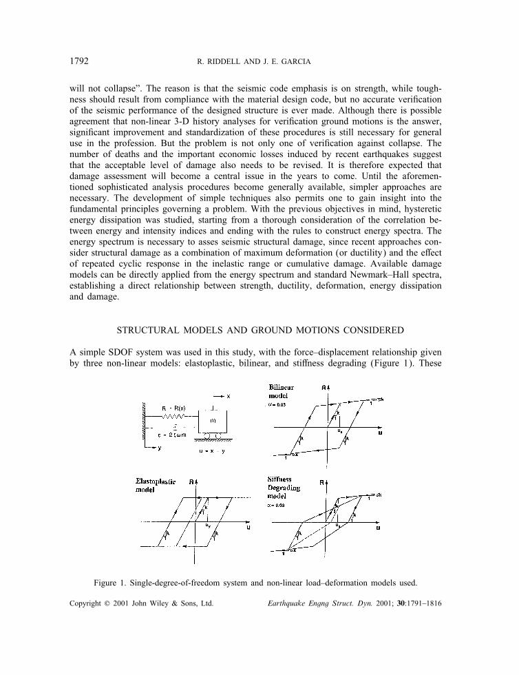
A simple SDOF system was used in this study, with the force–displacement relationship givenby three non-linear models: elastoplastic, bilinear, and sti?ness degrading (Figure 1). These

Figure 1. Single-degree-of-freedom system and non-linear load–deformation models used.

Copyright ? 2001 John Wiley & Sons, Ltd. Earthquake Engng Struct. Dyn. 2001; 30:1791–1816

HYSTERETIC ENERGY SPECTRUM AND DAMAGE CONTROL 1793

models cover a broad range of structural behaviour; they are intended to represent overallgeneric behaviour, rather than speci=c characteristics of individual systems [2; 3]. Strengthdeterioration was not considered, mainly because in a well-detailed structure it should onlyoccur at extreme deformations near the failure state. A damping factor �=0:05 (5 per centof critical) was used.

Fifty-two earthquake records were used as input ground motion (Table I). These recordsrepresent moderate-to-large intensities of motion. Damage was observed near the recordingsite of all these motions. Most of them satisfy the following intensity condition: peak groundacceleration larger than 0:25 g and=or peak ground velocity larger than 25 cm=sec. It was notattempted to group the records according to similar characteristics regarding soil conditions,tectonic environment, Mercalli Intensity, distance to fault, or others; the reason was in partthe lack of data—on geotechnical information for example—and the diOculty to form groupsof statistical signi=cance. Indeed, if families of similar characteristics could be arranged infuture studies, the scatter of results should decrease so that energy estimates could be mademore accurately. It must be pointed out, however, that the =ndings of the study may not bedirectly extrapolated to soft soils since most of the ground motion data considered is on =rmground.

EQUATION OF MOTION AND ENERGY EXPRESSIONS

The equation of motion of the system shown in Figure 1 can be written as

Qu(t) + 2�!u(t) +R(u)m

=− Qy(t) (1)

where u is the relative displacement of mass m with respect to its base, !=√

k=m is theundamped elastic circular frequency, R(u) is the hysteretic restoring force with sti?ness pa-rameter k (Figure 1), �= c=2!m is the damping factor as a fraction of the critical value,and Qy(t) is the base acceleration. Integrating Equation (1) with respect to u leads to thewell-known energy balance equation [4; 5] which must hold at any time during motion:

EK + ED + EH + ES =EI (2)

where, using du= u dt,

EK =∫ t

0Qu(t)u(t) dt=

12[u(t)2 − u(0)2] (3)

represents the kinetic energy per unit of mass, which becomes null if the initial velocity iszero and the integration is carried out long enough until the system comes to rest;

ED =2�!∫ t

0u2(t) dt (4)

is the energy per unit of mass dissipated by the viscous damper;

EH + ES =1m

∫ t

0R(u)u(t) dt (5)



Table I. Earthquakes records used in this study.

Station, component, date Maximum Maximum Maximumacceleration velocity displacement

(g) (cm=sec) (cm)

CMD Vernon, U.S.A. S08W (10=3=1933) −0:133 −29:03 −19:50El Centro, U.S.A. S00E (18=5=1940) −0:348 −33:45 −12:36Olympia, U.S.A. N86E (13=4=1949) 0.280 17.09 −9:38Eureka, U.S.A. N79E (21=12=1954) 0.258 −29:38 −12:55Ferndale, U.S.A. N44E (21=12=1954) −0:159 −35:65 14.72Kushiro Kisyo-Dai, Japan, N90E (23=4=1962) 0.478 −20:01 5.22Ochiai Bridge, Japan, N00E (5=4=1966) −0:276 23.66 8.36Temblor, U.S.A. S25W (27=6=1966) 0.348 −22:52 −5:55Cholame 2, U.S.A. N65E (27=6=1966) 0.489 78.08 −26:27Cholame 5, U.S.A. N85E (27=6=1966) 0.434 25.44 −6:89Lima, Peru, N08E (17=10=1966) 0.409 −15:20 −11:67El Centro, U.S.A. S00W (8=4=1968) 0.130 −25:81 12.96Hachinohe, Japan, N00E (16=5=1968) 0.269 −35:43 −9:68Aomori, Japan, N00E (16=5=1968) −0:257 −39:12 −19:97Muroran, Japan, N00E (16=5=1968) −0:220 30.28 7.90Itajima Bridge, Japan, Long. (6=8=1968) 0.612 −22:56 −4:59Itajima Bridge, Japan, Long. (21=9=1968) −0:261 −12:93 −2:80Toyohama Bridge, Japan, Long. (5=1=1971) 0.450 15.90 3.38Pacoima, U.S.A. S16E (9=2=1971) 1.171 113.23 −41:92Orion LA, U.S.A. N00W (9=2=1971) 0.255 30.00 16.53Castaic, U.S.A. N21E (9=2=1971) 0.316 17.16 −5:05Bucarest, Romania, S00E (4=3=1977) 0.206 75.12 −19:93San Juan, Argentina, S90E (23=11=1977) 0.193 −20:60 6.33Ventanas, Chile, Trans. (7=11=1981) 0.268 −17:87 −8:04Papudo, Chile, Long. (7=11=1981) −0:603 −18:93 −7:43La Ligua, Chile, Long. (7=11=1981) −0:469 −18:83 4.49Rapel, Chile, N00E (3=3=1985) 0.467 −21:64 −6:54Zapallar, Chile, N90E (3=3=1985) 0.304 13.46 −1:69Llo-Lleo, Chile, N10E (3=3=1985) −0:712 −40:29 −10:49Vina del Mar, Chile, S20W (3=3=1985) 0.363 30.74 −5:42UTFSM, Chile, N70E (3=3=1985) 0.176 14.60 3.11Papudo, Chile, S40E (3=3=1985) 0.231 12.41 1.60Llay Llay, Chile, S10W (3=3=1985) −0:352 −41:79 8.43San Felipe, Chile, N80E (3=3=1985) 0.434 −17:77 −3:50El Almendral, Chile, N50E (3=3=1985) 0.297 −28:58 −5:78Melipilla, Chile, N00E (3=3=1985) −0:686 34.25 12.02Pichilemu, Chile, N00E (3=3=1985) 0.259 −11:68 3.73Iloca, Chile, N90E (3=3=1985) 0.278 15.09 1.39SCT, Mexico, N90E (19=9=1985) −0:171 −60:61 21.16Corralitos, U.S.A. N00E (18=10=1985) 0.630 −55:20 12.03KSR Kushiro, Japan, N63E (15=1=1993) 0.725 33.59 4.73Pacoima DAM, U.S.A. S05E (17=1=1994) −0:415 44.68 4.65Newhall, U.S.A. N00E (17=1=1994) 0.591 −94:73 28.81Pacoima-Kagel, U.S.A. N00E (17=1=1994) 0.433 −50:88 −6:64Sylmar, U.S.A. N00E (17=1=1994) 0.843 −128:88 −30:67Santa Monica, U.S.A. N90E (17=1=1994) −0:883 41.75 −15:09

Continued



Table I. Continued

Station, component, date Maximum Maximum Maximumacceleration velocity displacement

(g) (cm=sec) (cm)

Moorpark, U.S.A. S00E (17=1=1994) 0.292 20.28 4.67Castaic, U.S.A. N90E (17=1=1994) 0.568 −51:51 −9:19Arleta, U.S.A. N90E (17=1=1994) 0.344 −40:37 8.36Century City-LA, U.S.A. N90E (17=1=1994) 0.256 21.36 −6:51Obregon Park-LA, U.S.A. N00E (17=1=1994) −0:408 −30:86 −2:65Hollywood-LA, U.S.A. N00E (17=1=1994) −0:389 22.26 4.27

is a term that composes the hysteretic energy EH, or energy dissipated per unit of mass byinelastic behaviour, and the stored elastic-strain energy per unit mass ES, which also vanisheswhen the system comes to rest; and

EI =−∫ u

0Qy(t) du=−

∫ t

0Qy(t)u(t) dt (6)

is the energy input per unit of mass, or energy supplied to the system by the moving base.Then, at the end of the motion, Equation (2) becomes

EH + ED =EI (7)

i.e. the total energy imparted to the structure by the earthquake must be dissipated by dampingand inelastic deformations.

CORRELATION BETWEEN ENERGY AND GROUND MOTION INTENSITY INDICES

The correlation between EI and EH and various indices that have been proposed to characterizethe intensity of earthquake motions was studied with the purpose of identifying appropriatenormalization or scaling parameters to derive energy spectra. It is well known that the inten-sity of motion cannot be satisfactorily characterized by a single parameter. Consequently, asin the case of response spectra, it was expected that di?erent intensity measures would be suit-able in the three characteristic spectral regions: short period (acceleration sensitive systems),intermediate period (velocity controlled responses) and long period (displacement sensitivesystems). Thus, a number of indices were considered as described next.

Arias [6; 7] proposed a measure of earthquake intensity that relates to the sum of theenergies dissipated, per unit of mass, by a population of damped oscillators of all naturalfrequencies (0¡!¡∞):

IA(�)=cos−1 �

g√

1− �2

∫ tf

0Qy2(t) dt (8)

where tf is the total duration of the ground motion and g is the acceleration of gravity. Housner[8] argued that a measure of seismic destructiveness could be given by the average rate ofbuildup of the total energy per unit mass input to structures; considering that the integral of



the squared ground acceleration was proportional to the total input energy, he proposed theearthquake power index

P=1

t1 − t2

∫ t2

t1Qy2(t) dt (9)

where t1 and t2 are the limits of the strong portion of motion. Mathematically, Equation (9)is the average value of the squared acceleration over the interval between t1 and t2. Thepopular de=nition of signi=cant duration of motion after Trifunac and Brady [9] was adoptedin this study, i.e. the interval between instants t5 and t95 at which 5 and 95 per cent of theintegral in Equation (8) is attained, respectively. Then the earthquake power, or mean-squareacceleration, is given by Equation (10), and similarly the indices mean-square velocity Pv andmean-square displacement Pd can be de=ned as given by Equations (11) and (12):

Pa =1

t95 − t5

∫ t95

t5Qy2(t) dt (10)

Pv =1

t95 − t5

∫ t95

t5y2(t) dt (11)

Pd =1

t95 − t5

∫ t95

t5y2(t) dt (12)

where y(t) and y(t) are the ground velocity and displacement histories, respectively. Hereafter,the signi=cant duration will be designated as td = t95 − t5. For simplicity, without regard toduration or to the constants involved in Equation (8), the integrals of the squared groundmotions have been used [10] as indices in the form:

Ea =∫ tf

0Qy2(t) dt (13)

Ev =∫ tf

0y2(t) dt (14)

Ed =∫ tf

0y2(t) dt (15)

The root-mean-square values of the ground motions, or e?ective values arms =√Pa, vrms =

√Pv,

and drms =√Pd have also been considered as potential measures of earthquake intensity [11–13]

as well as the square root of the integral of the squared ground motions: ars =√Ea, vrs =

√Ev,

and drs =√Ed.

Other indices, which are based on the previously discussed quantities and include newparameters, have been proposed as descriptors of earthquake intensity. Araya and Saragoni[14] de=ned the ‘potential destructiveness’ of an earthquake as

PD =IA�20

(16)

where IA is given by Equation (8) and �0 is the number of zero-crossings per unit of timeof the accelerogram; the signi=cance of this parameter is the incorporation of the frequency



content of the ground motion through �0. Park et al. [15] found that the ‘characteristic inten-sity’

IC = a1:5rmst

0:5d (17)

was a reasonable representation of the destructiveness of ground motions because it correlatedwell with structural damage expressed in terms of their damage index (Equation (37)). Fajfaret al. [16] proposed the expression

IF = vmaxt0:25d (18)

as a measure of the ground motion capacity to damage structures with fundamental periodsin the intermediate period range, wherein vmax is the peak ground velocity.

All the above indices depend only on the ground motions. They were used together with thepeak values of ground acceleration amax, ground velocity vmax, and ground displacement dmax totest their correlation with the input and hysteretic energies. Only one response-related parame-ter, Housner’s spectral intensity, was used as well. Since the pseudo-velocity response Sv andthe maximum strain energy stored in a linearly elastic system are related by ES max =mS2

v =2,Housner [17] argued that the spectrum itself was a measure of the severity of the earthquake,and de=ned the spectral intensity

SI(�)=∫ 2:5

0:1Sv(�; T ) dT (19)

Systems associated to three control frequencies 0.2, 1 and 5cps were chosen as representativeof the three characteristic spectral regions. Two types of energy were computed for each con-trol frequency: input energy for an elastic system, or energy dissipated by damping (EI =ED),and hysteretic energy EH dissipated by an inelastic system for a response associated to aductility factor �=3. Use of other values of � led to the same conclusions. To visualize thecorrelation among energy and the intensity indices, plots like Figure 2 were made for all theindices. In particular, Figure 2 shows the relation between index Ev (Equation (14)) and EH,where each asterisk corresponds to each of the 52 earthquake records; it can be seen that Ev

and EH correlate well for intermediate and low-frequency systems (1 and 0:2 cps), but theyshow no relation at all for 5 cps. To have an objective measure of the correlation, a curve ofthe form

E= �Q� (20)

was =tted to the data, where E is the energy, Q is the intensity index and � and � are thenon-linear regression parameters (or linear regression between the logarithms of the variables);the goodness of the =t is quanti=ed by the correlation coeOcient given by

�=n∑

(‘nQ ‘nE)−∑‘nQ

∑‘nE√

(n∑

(‘nQ)2 − (∑

‘nQ)2)(n∑

(‘nE)2 − (∑

‘nE)2)(21)

The correlation coeOcients for energy vs intensity, for all the indices, and for the three controlfrequencies, are summarized in Tables II and III; the indices ranked top-=ve for each frequencyare noted. The correlation coeOcient is the same for indices that di?er only by a constant orby the exponent. Several observations can be made from the results presented in these tables:



Figure 2. Hysteretic energy per unit of mass EH vs ground motion intensity index Ev forcontrol frequencies of 0.2, 1 and 5 cps.

(a) as expected, no index shows satisfactory correlation with energy in the three spectralregions simultaneously, indeed, acceleration related indices (amax; ars; arms; IC) are better forrigid systems (5 cps), velocity related indices (vmax; vrs; vrms; IF; SI) are better for intermediatefrequency systems (1 cps), and displacement related indices are better for Yexible systems(dmax; drs) although some velocity related indices also do well in the displacement region;(b) the peak ground motion parameters (amax; vmax; dmax) show good correlation, specially inthe displacement and acceleration regions where dmax and amax are the best, or nearly thebest indices; (c) considering the previous observation, and recalling that Nau and Hall [10]tested the same indices used herein (except PD; IC and IF) and found that none of them



Table II. Correlation coeOcient between input energy EI for elasticsystems and various intensity indices.

Index f = 0:2 cps f = 1 cps f = 5 cps

� Rank � Rank � Rank

dmax 0.862 2 0.469 0.244vmax 0.736 0.657 4 0.083amax 0.127 0.353 0.664 3Ed and drs 0.811 5 0.403 0.216Ev and vrs 0.905 1 0.785 2 0.029IA and Ea and ars 0.341 0.612 5 0.713 1Pd and drms 0.748 0.323 0.309Pv and vrms 0.761 0.574 0.091Pa and arms 0.139 0.294 0.514 4PD 0.685 0.553 0.156IC 0.289 0.536 0.693 2IF 0.817 4 0.772 3 0.039SI 0.842 3 0.792 1 0.012td 0.201 0.301 0.122

Table III. Correlation coeOcient between hysteretic energy EH for elastoplastic systems with responseductility � = 3 and various intensity indices.

Index f = 0:2 cps f = 1 cps f = 5 cps

� Rank � Rank � Rank

dmax 0.918 1 0.629 0.163vmax 0.750 0.781 4 0.108amax 0.027 0.276 0.817 2Ed and drs 0.886 2 0.531 0.249Ev and vrs 0.871 3 0.901 2 0.050IA and Ea and ars 0.175 0.549 0.786 3Pd and drms 0.839 4 0.478 0.201Pv and vrms 0.766 0.723 5 0.140Pa and arms 0.052 0.281 0.751 4PD 0.669 0.478 0.044IC 0.140 0.488 0.839 1IF 0.804 6 0.878 3 0.069SI 0.826 5 0.917 1 0.133td 0.129 0.245 0.110

provided noteworthy advantage over the peak ground motions to predict elastic and inelasticspectral ordinates, amax; vmax and dmax must be regarded as signi=cant intensity parameters tocharacterize the earthquake demand, and especially because they can be estimated for futureearthquakes with relative ease; (d) Housner’s intensity is the best index for f=1 cps, rankswell for f=0:2 cps, but does poorly for rigid systems; it should also be noted that SI is aresponse variable, hence, it is less desirable as a predictor variable; (e) similarly, Nau andHall [10] found that using Housner’s intensity as scaling parameter, but computed over threedi?erent ranges of frequency, provided less dispersion in the ordinates of normalized elastic



spectra than that which resulted from normalization to the peak ground motion parameters;however, the advantage faded away for inelastic systems with response ductilities larger than3; (f) although the duration of motion itself does not correlate well with input energy, nordissipated energy, it provides a signi=cant improvement of correlation when combined withother indices (Park’s index presents better correlation with energy than arms, and Fajfar’s indeximproves the correlation of vmax).

The previously discussed study permitted the narrowing down of the possibilities to a fewindices. Then two further analyses were carried out. First, examining the scatter of energyspectra (EH) computed for numerous frequencies, it was con=rmed that the above trendswere not limited to the particular control frequencies used, but actually extended to the entirefrequency range they were meant to represent. And second, considering the convenience ofincorporating td, new compound intensity indices of the form

I =Q 1 t 2d (22)

were evaluated. The exponents 1 and 2 were determined by means of an optimization scheme.The objective was to minimize, over the three relevant spectral regions, the average coeOcientof variation COV of energy spectra (EH) for the 52 records normalized using I as scalingparameter. The de=nition of COV will be presented in the next section. Exponents werecalculated for numerous cases: using the most promising intensity indices Q in the threespectral regions, for the three types of force–deformation relationships, and for =ve levels ofthe response ductility factor (1.5, 2, 3, 5 and 10). For each case, the optimization procedureconsisted of varying 1 and 2 in 0.1 increments starting from 1 = 2 = 0, computing COVfor each pair ( 1; 2) and plotting contour curves of COV. A typical example of such plotsis presented in Figure 3, where the optimum pair is approximately 1 = 0:75 and 2 = 0:35,for a minimum COV=0:43. It can be seen in Figure 3 that COV is not very sensitive to 1 and 2 since the surface COV( 1; 2) has small curvature in the vicinity of its minimumvalue. It was found that the indices Q in Equation (22) that led to smaller COVs were dmax

in the displacement region, vrms in the velocity region and amax and arms in the accelerationregion; however, using vrms instead of vmax produced less than 9 per cent reduction on COV,while using arms instead of amax resulted in negligible variation of COV for elastoplasticand bilinear systems and 13.6 per cent reduction for sti?ness degrading systems. Consideringthat recommendations to estimate the root-mean-square values of future ground motions arenot available, compound intensity indices including only the peak ground motion parametersdmax; vmax and amax are proposed. On the other hand, since COV is not very sensitive to 1and 2, and the optimum pairs ( 1; 2) are not signi=cantly di?erent when di?erent ductilitylevels and di?erent load–deformation relationships are considered, values 1 and 2 that canbe approximately applied for all cases were selected. Thus, the following compound intensityindices are recommended to normalize ground motions to predict energy dissipation duringearthquakes:

Id =dmaxt1=3d (23)

Iv = v2=3maxt1=3d (24)

Ia =

{amaxt

1=3d (25a)

amax (25b)



Figure 3. Contours of the average coeOcient of variation in the velocity region forenergy spectra normalized to v 1maxt

2d . Sti?ness degrading systems with 5 per cent

damping and response ductility �=3.

where Id applies in the displacement region of the spectrum for any load–deformation model,Iv applies in the velocity region for any model too, and Ia applies in the acceleration region,with Equation (25a) being suitable for sti?ness degrading models and Equation (25b) forelastoplastic or bilinear systems.

STATISTICAL ANALYSIS OF EH SPECTRA

Spectra of energy dissipated by inelastic behaviour EH were computed for the 52 recordslisted in Table I. An example is shown in Figure 4. It was found convenient to presentthe energy spectrum in terms of

√EH, because this quantity is linearly proportional to the

ground motion amplitude, i.e. if the ground acceleration is ampli=ed by a factor ! the energyspectrum is ampli=ed by the same factor. At the same time, since the yield levels of theinelastic systems are taken as a fraction of the elastic response displacement, when a recordis ampli=ed by a factor ! and the yield level is ampli=ed by the same factor, the responseductility factor is the same as that of a system with the non-ampli=ed load–deformationrelationship subjected to the non-ampli=ed motion. In turn, since EH corresponds to dissipatedenergy per unit of mass,

√EH has velocity units and the three axes of the tri-partite logarithmic

plot have the same units of the conventional response spectrum. Therefore, it is appropriate to



Figure 4. Dissipated energy spectrum for the Sylmar N00E record of 17 January 1994. Sti?nessdegrading systems with 5 per cent damping.

refer to the three regions of the energy spectrum as displacement, velocity, and accelerationregions.

As a =rst step, average spectra are computed. Designating the energy spectrum as

SH =√

EH = SH(f; �; �; R(u)) (26)

the normalized average spectrum is given by

ZSH(f)=1n

n∑i=1

SHi(f)Ii

(27)

where f is the frequency (f=!=2#), Ii is the normalization factor for the ith record, nis the number of records and SHi is the ith spectrum for given values of � and � and fora given restoring-force model. Average energy spectra for sti?ness degrading systems arepresented in Figures 5, 6 and 7, for spectra normalized to the indices dmax; v2=3max and amax,respectively; each =gure is pertinent only in the frequency range that corresponds to thescaling index used. The shapes of the average spectra for elastoplastic and bilinear systemsare similar to those shown in these =gures. It can be observed that: (a) for low frequencies,and for a given value of �,

√EH=! slightly increases with !, it does not vary signi=cantly

with �, and it is approximately equal to the peak ground displacement dmax (Figure 5); (b)



Figure 5. Average energy spectra for records normalized to peak ground displacement (dmax). Sti?nessdegrading systems with 5 per cent damping.

for intermediate frequencies (Figure 6),√EH does not vary signi=cantly with � either, but

increases as ! increases; and (c) for high frequencies (Figure 7), !√EH decreases as !

increases, but increases with �. The average spectra suggest an energy spectrum shaped asshown in Figure 8. Note that the trilinear spectrum is not parallel to the three axes of thetripartite logarithmic plot.

The next step is to compute the corner frequencies fdv and fva (Figure 8) that de=ne thethree spectral regions. Lower and upper limits of 0.05 and 20 cps were arbitrarily chosen asboundaries of the frequency range of practical interest. The trilinear spectrum is de=ned inthe logarithmic space by exponential curves

$d = %df&d (28a)

$v = %vf&v (28b)

$a = %af&a (28c)

where the six regression coeOcients % and & are determined by minimizing the square errorbetween the trilinear spectrum $ and the average energy spectrum ZSH (Equation (27)) in eachspectral region:

[2 =nf∑j=1

wj[ ZSH(fj)− $(fj)]2 (29)



Figure 6. Average energy spectra for records normalized to v2=3max. Sti?ness degradingsystems with 5 per cent damping.

where nf is the number of frequencies, wj =0:5(fj+1 − fj−1)=(fu − f‘) is a weight factor toaccount for unequally spaced frequencies, and f‘ and fu are the lower and upper frequenciesof the corresponding spectral region. The iterative procedure begins with assumed values ofthe corner frequencies, and new values are computed in each cycle. The conditions $v =!dv$dand $a =!va$v hold at the corner frequencies fdv and fva; respectively (with !dv =2#fdv and!va =2#fva). Thus, using Equations (28), the corner frequencies are

f(i)dv =

[%(i)v

2#%(i)d

](1

1+&(i)d −&(i)v

)(30a)

f(i)va =

[%(i)a

2#%(i)v

](1

1+&(i)v −&(i)a

)(30b)

where i denotes the ith cycle. The procedure converges rapidly until f(i+1) is as close tof(i) as desired at each corner. The =nal step is to compute statistics in each spectral region,for each ductility factor, and for each restoring force model. The variance and the standard



Figure 7. Average energy spectra for records normalized to peak ground acceleration (amax). Sti?nessdegrading systems with 5 per cent damping.

Figure 8. Shape of the smoothed spectrum of energy dissipation.



deviation are de=ned as

VAR($) =1n

n∑i=1

∫ fuf‘[SHi(f)=Ii − $(f)]2 df

fu − f‘(31)

)($) =√

VAR($) (32)

where i denotes the ith record, and n is the number of records. In turn, as mentioned in theprevious section, for the evaluation of the compound intensity indices, the average coeOcientof variation over a spectral region was computed as

COV($)=∑jwj COV[$(fj)] (33)

where COV[$(fj)] is the discrete coeOcient of variation for each frequency in the regiongiven by

COV[$(fj)]=1

$(fj)

√1n∑i[SHi(fj)=Ii − $(fj)]2 (34)

The =nal results of the method outlined above are summarized in Tables IV, V and VI forthe elastoplastic, bilinear and sti?ness degrading models, respectively. These tables give thecoeOcients % and & (Equation (28)) and statistics according to Equations (32) and (33); inaddition to the results associated with normalization to the indices given by Equations (23)–(25), which produce the least dispersion, the results related to normalization by the peakground motion parameters with no regard to td are also provided.

The calculated statistics are based on the assumption that the square root of the energydissipated per unit of mass (

√EH) is normally distributed. The assumption is sound if the

derived probability distribution for EH; the variable of interest, presents good =t with the actualresponse data. The =tness was checked applying the Kolmogorov–Smirnov test at three controlfrequencies that presented the most scatter; it was found that the test satis=ed a signi=cancelevel of 5 per cent by an ample margin.

As a part of the study, factors for constructing elastic and inelastic design spectra were alsoobtained. The procedure due to Veletsos–Newmark–Hall-Mohraz [18–23] and later revised byRiddell–Newmark [3; 24] is well known. Indeed, the method is simpler than the extensionto energy spectra presented above, because the ordinates of the trilinear design spectrum, inthe region response ampli=cation, are parallel to the corresponding axes of the tripartite grid.Factors for elastoplastic systems with 5 per cent damping are presented in Table VII. Thesefactors can be conservatively used for bilinear and sti?ness degrading systems, since on theaverage the ductility demand on them is less than that imposed on elastoplastic systems, asearlier reported [3; 25] and con=rmed in this work. The ordinates of the design spectrum S�for given ductility factor � are obtained applying the ampli=cation factors � (Table VII) tothe corresponding peak ground motion parameters pg:

S� = �pg (35)



Table IV. Factors for constructing energy dissipation spectra (EH) for elastoplasticsystems with 5 per cent damping.

Spectral region and Ductility $� = %�f&� Standard deviation COV�normalization index

� %� &� )�

Displacement dmaxt1=3d 1.5 0.58 0.18 0.17 0.382 0.60 0.11 0.18 0.343 0.59 0.04 0.17 0.315 0.53 −0:14 0.17 0.31

10 0.44 −0:05 0.16 0.34

Displacement dmax 1.5 1.49 0.20 0.44 0.382 1.58 0.13 0.50 0.373 1.53 0.06 0.55 0.385 1.38 −0:01 0.59 0.42

10 1.15 −0:04 0.57 0.48

Velocity v2=3maxt1=3d 1.5 1.28 0.15 0.82 0.57

2 1.55 0.17 0.94 0.533 1.75 0.18 0.99 0.485 1.85 0.17 0.99 0.45

10 1.88 0.14 0.93 0.42

Velocity v2:3max 1.5 3.20 0.13 2.13 0.602 3.88 0.15 2.50 0.573 4.42 0.15 2.78 0.555 4.74 0.15 2.90 0.53

10 4.86 0.13 2.83 0.51

Acceleration amax 1.5 3.56 −0:48 0.49 0.382 4.40 −0:44 0.65 0.383 5.16 −0:39 0.84 0.385 5.50 −0:29 1.06 0.38

10 5.73 −0:18 1.31 0.35

where pg represents dmax, vmax, or amax depending on the spectral region of interest. The elasticspectrum Se is given by Equation (35) for the particular case �=1; wherefrom the inelasticspectrum can be alternatively obtained as

S� =,�Se (36)

where ,� is also given in Table VII. It is worth commenting here that Equation (36) is of-ten misunderstood as equivalent to ‘deriving inelastic spectra from elastic response analyses’.This is certainly not the case because actual inelastic responses directly lead to the � factors(average ampli=cation with respect to the peak ground motion parameters). Simple approx-imations for ,� are well known: the ratios 1=� for the displacement and velocity regions,and 1=

√2� − 1 for the acceleration region (which were shown [3] to be unconservative for

high ductility and high damping, as also apparent in this study). Table VII also providesthe standard deviation )� and the coeOcient of variation COV=)�= � calculated over thecorresponding spectral regions.



Table V. Factors for constructing energy dissipation spectra (EH) for bilinearsystems with 5 per cent damping.


� %� &� )�

Displacement dmaxt1=3d 1.5 0.59 0.19 0.17 0.382 0.62 0.12 0.18 0.333 0.59 0.04 0.17 0.315 0.51 −0:03 0.17 0.31

10 0.41 −0:08 0.14 0.34

Displacement dmax 1.5 1.52 0.21 0.44 0.382 1.61 0.14 0.50 0.373 1.53 0.06 0.56 0.395 1.33 −0:02 0.58 0.43

10 1.05 −0:08 0.53 0.48

Velocity v2=3maxt1=3d 1.5 1.29 0.16 0.84 0.58

2 1.56 0.18 0.96 0.543 1.77 0.18 1.01 0.485 1.89 0.15 0.98 0.44

10 1.88 0.14 0.89 0.40

Velocity v2=3max 1.5 3.22 0.14 2.22 0.622 3.93 0.16 2.63 0.593 4.51 0.16 2.88 0.565 4.85 0.13 2.91 0.53

10 4.86 0.12 2.76 0.50


10 5.95 −0:13 1.59 0.37

The COV values in Table VII are consistent with previous studies. Riddell and Newmark[3] found COVs in the range 0.18–0.22 in the acceleration region of the spectrum, 0.31–0.39in the velocity region and 0.41–0.49 in the displacement region, for � between 1 and 10, whileRiddell [25] obtained COVs between 0.19–0.31, 0.25–0.4, and 0.33–0.44 in the mentionedregions respectively, for the same damping and range of �. Miranda [26] and Riddell [25] havereported COV values for the response modi=cation factor R� (R�, the ratio between elasticand inelastic response, is a close relative of ,�, the former being calculated for individualfrequencies while the latter is a frequency-band ratio). Miranda [26] found COV(R�) varyingbetween about 0.25 and 0.45 for groups of records on rock and alluvial soils, for � between2 to 6, with COV increasing as ductility increased; Riddell [25] obtained practically the sameCOVs for R�. It is worth recalling that Miranda [26] and Riddell [25] considered earthquakerecords grouped according to soil conditions and thus the dispersion should decrease due tothe similar frequency content of the motions, whereas in this study a wide variety of groundmotions regarding soil conditions and tectonic settings were used. In a recent study, Ordaz



Table VI. Factors for constructing energy dissipation spectra (EH) for sti?ness degradingsystems with 5 per cent damping.


� %� &� )�

Displacement dmaxt1=3d 1.5 0.69 0.21 0.18 0.342 0.66 0.14 0.17 0.303 0.56 0.06 0.16 0.295 0.46 0.01 0.13 0.29

10 0.34 −0:04 0.10 0.30

Displacement dmax 1.5 1.78 0.22 0.50 0.372 1.69 0.15 0.52 0.363 1.44 0.07 0.50 0.375 1.17 0.01 0.45 0.39

10 0.88 −0:03 0.36 0.40

Velocity v2=3maxt1=3d 1.5 1.67 0.17 1.00 0.52

2 1.85 0.18 1.04 0.483 1.91 0.18 1.00 0.445 1.87 0.18 0.92 0.40

10 1.75 0.18 0.83 0.37

Velocity v2=3max 1.5 4.24 0.15 2.84 0.592 4.70 0.16 3.02 0.553 4.88 0.16 2.97 0.525 4.81 0.16 2.83 0.49

10 4.54 0.17 2.61 0.47

Acceleration amaxt1=3d 1.5 2.18 −0:41 0.41 0.492 2.39 −0:33 0.50 0.463 2.37 −0:21 0.60 0.425 2.27 −0:08 0.71 0.38

10 2.12 −0:06 0.83 0.34


10 5.54 0.05 2.62 0.42

and Perez [27] proposed rules to predict R� that featured better accuracy than other availablerelationships; it should be noted, though, that they predicted R� on the basis of responsequantities: the relative velocity spectrum and=or the displacement response spectrum. Thefactors in Tables IV–VII, however, are predicted on the basis of a priori parameters: the peakground motion parameters or other ground motion intensity indices. COV (average COV) ofhysteretic energy spectra in the displacement and acceleration regions can be held in the range0.3–0.5 if the appropriate normalization index is used (indices including td). The larger COVin the velocity region could be reduced if vrs o vrms were used instead of vmax; as mentionedabove; however, estimates of the former indices for future earthquakes are not available and



Table VII. Factors for constructing elastic and inelastic design spectra for systems with 5 per centdamping.

Spectral region and Ductility � � )� COV ,�normalization index

Displacement dmax 1 1.76 0.77 0.44 1.001.5 1.07 0.45 0.42 0.612 0.76 0.32 0.42 0.433 0.50 0.23 0.45 0.295 0.30 0.14 0.46 0.17

10 0.15 0.07 0.48 0.08

Velocity vmax 1 1.67 0.78 0.46 1.001.5 1.05 0.42 0.40 0.622 0.78 0.31 0.40 0.473 0.54 0.21 0.39 0.325 0.36 0.14 0.37 0.22

10 0.22 0.08 0.36 0.13

Acceleration amax 1 2.09 0.71 0.34 1.001.5 1.46 0.38 0.26 0.702 1.23 0.28 0.23 0.593 1.02 0.22 0.21 0.495 0.84 0.18 0.21 0.40

10 0.67 0.16 0.24 0.32

so the latter was preferred. If v2=3maxt1=3d is used as recommended (Equation (24)), COV in the

velocity region ranges between 0.37 and 0.58. Such a range denotes large uncertainty but itis not extraordinarily larger than the above-commented values.

CONSTRUCTION OF DISSIPATED ENERGY SPECTRA AND APPLICATION TODAMAGE CONTROL

The =rst step in the construction of energy and design spectra involves the de=nition of theearthquake hazard in terms of estimates of the expected peak ground motion parameters atthe site under consideration. A discussion of this subject is beyond the scope of this paper.The spectra presented in this section will be anchored to a peak ground acceleration of 1g;which is only a referential value selected for illustrative purposes and has no e?ect on theobservations to be made. The design peak ground velocity and displacement will be de=nedon the basis of average values of the ratios vmax=amax and amaxdmax=v2max. In this study, meanvalues of 98:5cm=sec=g and 4 were obtained for the previously mentioned ratios, while Riddelland Newmark [3] found averages of 89 and 6, respectively. Assuming vmax=amax =85 andamaxdmax=v2max =6; vmax =85 cm=sec and dmax =44 cm are obtained. Next, energy dissipationspectra and inelastic spectra required for damage assessment will be constructed. Spectra forelastoplastic systems with 5 per cent damping and response ductility �=5 will be considered.



Energy spectrum

Assuming that no estimate of the ground motion duration td is available, the design groundmotion (Figure 8) for constructing the energy spectrum (ES) is simply taken as dmax =44cm,v2=3max =852=3 = 19 cm=sec; and amax =1g. The factors to determine the spectral ordinates aregiven in Table IV. Supposing that some degree of conservatism is desired, factors asso-ciated with the mean plus one standard deviation level will be used (15.9 per cent prob-ability of exceedance). Thus, the spectral ampli=cation factors for �=5 are $d =(1:38 +0:59)f−0:01 = 1:97f−0:01 in the displacement region, $v =(4:74+2:9)f0:15 = 7:64f0:15 in the ve-locity region, and $a =(5:5+1:06)f−0:29 = 6:56f−0:29 in the acceleration region. For f=0:05;the lowest frequency of the spectrum (Figure 8), the ampli=cation factor $d =2:03 is ob-tained; then

√EH=!=dmax$d =89 cm determines point J of the spectrum (Figure 8). Sim-

ilarly, for f=20; $a =2:75 gives !√EH =2:75amax =2:75g which corresponds to point M

(Figure 8). The corner frequency fdv is calculated from the condition dmax$d!= v2=3max$v i.e.,86:7f−0:01!=145:2f0:15 which yields fdv =0:207 and

√EH = v2=3max$v =145:2(0:207)0:15 =

115 cm=sec (point K in Figure 8). The corner frequency fva results from v2=3max$v!= amax$a;i.e. 145:2f0:15!=6433f−0:29; wherefrom fva =3:882cps and

√EH = v2=3max$v =145:2(3:882)0:15 =

178 cm=sec (point L in Figure 8). The completed trilinear energy spectrum is plotted in Fig-ure 9, for which the relevant labels of the tripartite grid axes are

√EH=!,

√EH; and !

√EH

in the displacement, velocity, and acceleration regions, respectively. It can be seen in Fig-ure 9 that the energy dissipation demand varies considerably with frequency. At the peak ofthe smoothed energy spectrum (f=3:88 cps) EH =31684 cm2=sec2 while at the ends of thespectrum EH is 780 and 460 cm2=sec2; respectively, i.e. ratios of the order of 40 and 70,respectively.

Inelastic spectra

As selected above, the design ground motion parameters are dmax =44 cm; vmax =85 cm=sec;and amax =1g. In this case, the spectrum to be constructed =rst is the inelastic yield spectrum[3] (IYS), also known as constant-ductility spectrum [28], which corresponds to a plot ofthe yield deformation uy necessary to limit the maximum deformation of the system to aspeci=ed multiple of the yield deformation itself (umax =�uy). Since the factors given inTable VII synthesize the characteristics of a family of 52 earthquake records, the spectrumcorresponds to a smoothed design spectrum, in opposition to a response spectrum that refersto the response to one speci=c excitation. In this case, the spectral quantities of interestare uy in the displacement axis and !2uy in the acceleration axis; the latter multiplied bythe mass gives the yield resistance Fy of the system, which in the case of an elastoplasticsystem is also its maximum strength. In the ampli=ed region of the spectrum, between 0.15and 10 cps; the spectral ordinates are obtained using the mean-plus-one-standard-deviation( �+)�) factors given in Table VII for �=5: 0.44, 0.5 and 1.02 for the displacement, velocity,and acceleration regions, respectively. Thus, the spectral ordinates are: 44× 0:44=19 cm;85× 0:5=43 cm=sec and 1g× 1:02=1:02g. The spectrum is completed with transition zones:in the lowest frequency (0:05cps) the spectral ordinate is dmax=�=44=5=8:8cm; in the highestfrequency (33cps) the spectral ordinate is [3] amax�−0:07 = 0:89g. The complete inelastic designspectrum is presented in Figure 9. The second spectrum of interest is the total deformation



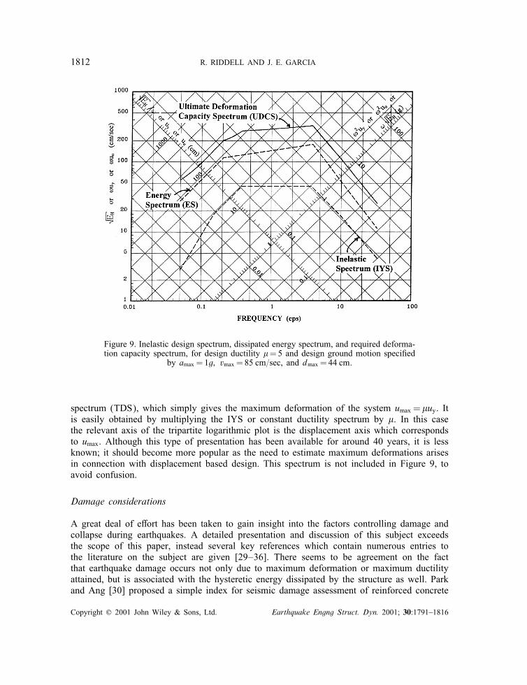
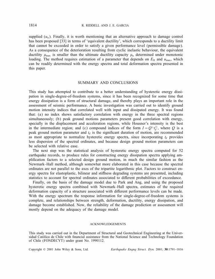
Figure 9. Inelastic design spectrum, dissipated energy spectrum, and required deforma-tion capacity spectrum, for design ductility �=5 and design ground motion speci=ed

by amax = 1g; vmax = 85 cm=sec, and dmax = 44 cm.

spectrum (TDS), which simply gives the maximum deformation of the system umax =�uy. Itis easily obtained by multiplying the IYS or constant ductility spectrum by �. In this casethe relevant axis of the tripartite logarithmic plot is the displacement axis which correspondsto umax. Although this type of presentation has been available for around 40 years, it is lessknown; it should become more popular as the need to estimate maximum deformations arisesin connection with displacement based design. This spectrum is not included in Figure 9, toavoid confusion.

Damage considerations

A great deal of e?ort has been taken to gain insight into the factors controlling damage andcollapse during earthquakes. A detailed presentation and discussion of this subject exceedsthe scope of this paper, instead several key references which contain numerous entries tothe literature on the subject are given [29–36]. There seems to be agreement on the factthat earthquake damage occurs not only due to maximum deformation or maximum ductilityattained, but is associated with the hysteretic energy dissipated by the structure as well. Parkand Ang [30] proposed a simple index for seismic damage assessment of reinforced concrete



structures:

DPA =umax

uu+ �

mEH

Fyuu(37)

where umax is the maximum deformation under earthquake excitation (as de=ned above), uu isthe ultimate deformation capacity under monotonic loading, Fy is yield resistance (as de=nedabove), mEH is the total hysteretic energy dissipation, � is a parameter that weights the e?ectof cyclic loading on structural damage and DPA¿1 means complete collapse or total damage.Note that umax=uu would be equal to 1 if umax was measured in a monotonic loading test, inturn mEH=Fyuu would also equal 1 under such a test. The clear implication of Equation (37)is that, under earthquake loading, when energy dissipation takes place, umax cannot reach uu.Values of � based on experimental data [30] varied between −0:3 and 1.2, with a median[35] of 0.15. Since the latter value has been also used by other authors [30; 34–36], �=0:15will be taken for the following example. Further elaboration on appropriate values of � fordi?erent structural materials and con=gurations is probably needed.

Using the energy spectra presented herein combined with Newmark–Hall spectra, a simpleestimation of the required deformation capacity of a structure can be made. Indeed, takingDPA =1; the ultimate deformation capacity supplied to the structure must comply with

uu¿umax + �mEH

Fy(38)

recalling that uu is the design capacity based on monotonic testing data and monotonic be-haviour knowledge, while the second member of Equation (38) corresponds to earthquakeresponse quantities. The latter quantities are directly read from the spectra presented above;in fact, umax is the TDS, Fy=m is the IYS but read in the acceleration axis (or IYS ·!2 if readin the displacement axis), and EH is the ES squared. In symbolic form, for each frequency,Equation (38) can be written as

UDCS¿TDS + �ES2

IYS(39)

where UDCS is the ultimate deformation capacity spectrum. In other words, UDCS gives therequired monotonic deformation capacity for the structure to survive the design earthquakewithout collapse. The UDCS is plotted in Figure 9 according to Equation (39); naturallyit is read in the displacement axis. Note also that di?erent levels of acceptable damage,i.e. performance, may be established by taking di?erent values of DPA; for example takingDPA =0:5 the design condition given by Equation (38) becomes

uu¿2(umax + �

mEH

Fy

)(40)

The appeal of this expression is that the quantity in parenthesis in the second member doesnot change, i.e. it is obtained from the same design spectra based on the same design groundmotion, but certainly the structure should be provided more displacement capacity if betterperformance is desired. The implication is that performance based design need not be speci=edthrough a set of ground motions of di?erent intensities, but through one design motion withperformance controlled by the design parameters selected (Fy or �) and deformation capacity



supplied (uu). Finally, it is worth mentioning that an alternative approach to damage controlhas been proposed [33] in terms of ‘equivalent ductility’, which corresponds to a ductility limitthat cannot be exceeded in order to satisfy a given performance level (permissible damage).As a consequence of the deterioration resulting from cyclic inelastic behaviour, the equivalentductility �max is smaller than the ultimate ductility capacity �u determined under monotonicloading. The method requires estimation of a parameter that depends on EH and umax; whichcan be readily determined with the energy spectra and total deformation spectra presented inthis paper.

SUMMARY AND CONCLUSIONS

This study has attempted to contribute to a better understanding of hysteretic energy dissi-pation in single-degree-of-freedom systems, since it has been recognized for some time thatenergy dissipation is a form of structural damage, and thereby plays an important role in theassessment of seismic performance. A basic investigation was carried out to identify groundmotion intensity indices that correlated well with input and dissipated energy. It was foundthat: (a) no index shows satisfactory correlation with energy in the three spectral regionssimultaneously; (b) peak ground motions parameters present good correlation with energy,specially in the displacement and acceleration regions, while Housner’s intensity is the bestin the intermediate region; and (c) compound indices of the form I =Q 1 t 2d ; where Q is apeak ground motion parameter and td is the signi=cant duration of motion, are recommendedas most appropriate to normalize hysteretic energy spectra, since incorporating td providesless dispersion of the spectral ordinates, and because design ground motion parameters canbe selected with relative ease.

The next step was the statistical analysis of hysteretic energy spectra computed for 52earthquake records, to produce rules for constructing energy dissipation spectra applying am-pli=cation factors to a selected design ground motion, in much the similar fashion as theNewmark–Hall method, although somewhat more elaborated in this case because the spectralordinates are not parallel to the axes of the tripartite logarithmic plot. Factors to construct en-ergy spectra for elastoplastic, bilinear and sti?ness degrading systems are presented, includingstatistics to account for spectral ordinates associated to di?erent probabilities of exceedance.

Finally, on the basis of the damage model due to Park and Ang, and using the proposedhysteretic energy spectra combined with Newmark–Hall spectra, estimates of the requireddeformation capacity of a structure associated with di?erent performance levels can be made.With the energy spectrum the response information for single-degree-of-freedom systems iscomplete, and relationships between strength, deformation, ductility, energy dissipation, anddamage become established. Now, the reliability of the damage prediction or assessment willmostly depend on the adequacy of the damage model.

ACKNOWLEDGEMENTS

This study was carried out in the Department of Structural and Geotechnical Engineering at the Univer-sidad CatGolica de Chile with =nancial assistance from the National Science and Technology Foundationof Chile (FONDECYT) under grant No. 1990112.



REFERENCES

1. Blume JA, Newmark NM, Corning LH. Design of multistory reinforced concrete buildings for earthquakemotions. Portland Cement Association, Skokie, IL, 1961.

2. Riddell R, Newmark NM. Force–deformation models for nonlinear analysis. Journal of the Structural Division,ASCE 1979; 105(ST12):2773–2778.

3. Riddell R, Newmark NM. Statistical analysis of the response of nonlinear systems subjected to earthquakes.Structural Research Series No. 468, Department of Civil Engineering, University of Illinois, Urbana, IL, 1979.

4. Kato B, Akiyama H. Energy input and damages in structures subjected to severe earthquakes. A.I.J, No. 235,1975.

5. Zahrah T, Hall WJ. Seismic energy absorption in simple structures, Structural Research Series No. 501,Department of Civil Engineering, University of Illinois, Urbana, IL, 1982.

6. Lange JG. Una medida de intensidad sG\smica. Departamento de Obras Civiles, Universidad de Chile, Santiago,Chile, 1968.

7. Arias A. A measure of earthquake intensity. Seismic Design for Nuclear Power Plants. MIT Press: Cambridge,1970.

8. Housner GW. Measures of severity of earthquake ground shaking. Proceedings of the U.S. National Conferenceon Earthquake Engineering, EERI, Ann Arbor, MI, 1975.

9. Trifunac MD, Brady AG. A study on the duration of strong earthquake ground motion. Bulletin of theSeismological Society of America 1975; 65(3):581–626.

10. Nau JM, Hall WJ. An evaluation of scaling methods for earthquake response spectra. Structural ResearchSeries No. 499, Department of Civil Engineering, University of Illinois, Urbana, IL, 1982.

11. Housner GW, Jennings PC. Generation of arti=cial earthquakes. Journal of the Engineering Mechanics Division,ASCE 1964; 90(EM1):113–150.

12. Housner GW. Strong ground motion. In Earthquake Engineering, chapter 4. Wiegel RL (ed.). Prentice-HallInc.: Engelwood Cli?s, NJ, 1970.

13. Housner GW. Design spectrum. In Earthquake Engineering, chapter 5. Wiegel RL (ed.). Prentice-Hall Inc.:Engelwood Cli?s, NJ, 1970.

14. Araya R, Saragoni R. Capacidad de los movimientos sG\smicos de producir dano estructural. SES I 7=80 (156),Universidad de Chile, Santiago.

15. Park Y-J, Ang AH-S, Wen YK. Seismic damage analysis of reinforced concrete buildings. Journal of StructuralEngineering, ASCE 1985; 111(4):740–757.

16. Fajfar P, Vidic T, Fischinger M. A measure of earthquake motion capacity to damage medium-period structures.Soil Dynamics and Earthquake Engineering 1990; 9(5).

17. Housner GW. Spectrum intensities of strong motion earthquakes. Proceedings of the Symposium on Earthquakeand Blast E/ects on Structures, EERI, California, 1952.

18. Veletsos AS, Newmark NM. E?ect of inelastic behavior on the response of simple systems to earthquakemotions. Proceedings of the 2WCEE, vol. 2, Japan, 1960.

19. Veletsos AS, Newmark NM. Response spectra for single-degree-of-freedom elastic and inelastic systems. ReportNo. RTD-TDR-63-3096, vol. III, Air Force Weapons Laboratory, Albuquerque, NM, 1964.

20. Veletsos AS. Maximum deformation of certain nonlinear systems. Proceedings of the Fourth WCEE, vol. I,Chile, 1969.

21. Newmark NM, Hall WJ. Seismic design criteria for nuclear reactor facilities. Proceedings of the Fourth WCEE,vol. 3, Chile, 1969.

22. Newmark NM, Hall WJ, Mohraz B. A study of vertical and horizontal earthquake spectra. U.S. Atomic EnergyCommission Report WASH-1225, Washington D.C., 1973.

23. Newmark NM, Hall WJ. Procedures and criteria for earthquake resistant design. Building Practices for DisasterMitigation, National Bureau of Standards, Building Science Series No. 46, 1973.

24. Riddell R. E?ect of damping and type of material nonlinearity on earthquake response. Proceedings of theSeventh WCEE, vol. 4, Turkey, 1980.

25. Riddell R. Inelastic design spectra accounting for soil conditions. Earthquake Engineering and StructuralDynamics 1995; 24(11):1491–1510.

26. Miranda E. Site-dependent strength-reduction factors. Journal of Structural Engineering, ASCE 1993;119(12):3503–3519.

27. Ordaz M, Perez-Rocha L. Estimation of strength-reduction factors for elastoplastic systems: a new approach.Earthquake Engineering and Structural Dynamics 1998; 27(9):889–901.

28. Chopra AK. Dynamics of Structures. Prentice-Hall Inc.: Engelwood Cli?s, NJ, 1995.29. Banon H, Veneziano D. Seismic safety of reinforced concrete members and structures. Earthquake Engineering

and Structural Dynamics 1982; 10:179–193.30. Park Y-J, Ang AH-S. Mechanistic seismic damage model for reinforced concrete. Journal of Structural

Engineering, ASCE 1985; 111(4):722–739.



31. Zhu TJ, Tso WK, Heidebrecht AC. E?ect of peak ground a=v ratio on structural damage. Journal of StructuralEngineering, ASCE 1988; 114(5):1019–1037.

32. McCabe SL, Hall WJ. Assessment of seismic structural damage. Journal of Structural Engineering, ASCE1989; 115(9):2166–2183.

33. Fajfar P. Equivalent ductility factors taking into account low-cycle fatigue. Earthquake Engineering andStructural Dynamics 1992; 21:837–848.

34. Cosenza E, Manfredi G, Ramasco R. The use of damage functions in earthquake engineering: a comparisonbetween di?erent methods. Earthquake Engineering and Structural Dynamics 1993; 22:855–868.

35. Chai YH, Romstad KM, Bird SM. Energy-based linear damage model for high intensity seismic loading. Journalof Structural Engineering, ASCE 1995; 121(5):857–864.

36. Krawinkler H. Performance assessment of steel components. Earthquake Spectra 1987; 3:22–41.


Riddell Garcia

Documents

Transcript of Riddell Garcia