1

Rich Models for Steganalysis of Digital ImagesJessica Fridrich, Member, IEEE and Jan Kodovský

Abstract—We describe a novel general strategy forbuilding steganography detectors for digital images.The process starts with assembling a rich model of thenoise component as a union of many diverse submodelsformed by joint distributions of neighboring samplesfrom quantized image noise residuals obtained usinglinear and non-linear high-pass filters. In contrast toprevious approaches, we make the model assembly apart of the training process driven by samples drawnfrom the corresponding cover- and stego-sources. En-semble classifiers are used to assemble the model aswell as the final steganalyzer due to their low com-putational complexity and ability to efficiently workwith high-dimensional feature spaces and large trainingsets. We demonstrate the proposed framework on threesteganographic algorithms designed to hide messages inimages represented in the spatial domain: HUGO, edge-adaptive algorithm by Luo et al. [32], and optimally-coded ternary ±1 embedding. For each algorithm, weapply a simple submodel-selection technique to in-crease the detection accuracy per model dimensionalityand show how the detection saturates with increasingcomplexity of the rich model. By observing the differ-ences between how different submodels engage in detec-tion, an interesting interplay between the embeddingand detection is revealed. Steganalysis built around richimage models combined with ensemble classifiers is apromising direction towards automatizing steganalysisfor a wide spectrum of steganographic schemes.

I. IntroductionModern feature-based steganalysis starts with adopting

an image model (a low-dimensional representation) withinwhich steganalyzers are built using machine learning tools.The model is usually determined not only by the char-acteristics of the cover source but also by the effects ofembedding [4], [6], [14], [18], [21], [33], [35], [38]. For ex-ample, the SPAM feature vector [33], which was seeminglyproposed from a pure cover model, is in reality, too, drivenby a specific case of steganography. The choice of the orderof the Markov process as well as the threshold T and the

The work on this paper was supported by the Air Force Office ofScientific Research under the research grant FA9550-09-1-0147. TheU.S. Government is authorized to reproduce and distribute reprintsfor Governmental purposes notwithstanding any copyright notationthere on. The views and conclusions contained herein are those of theauthors and should not be interpreted as necessarily representing theofficial policies, either expressed or implied of AFOSR or the U.S.Government.

The authors would like to thank Vojtěch Holub for useful discus-sions.

The authors are with the Department of Electrical and Com-puter Engineering, Binghamton University, NY, 13902, USA. Email:fridrich@binghamton.edu, jan.kodovsky@binghamton.edu.

Copyright (c) 2012 IEEE. Personal use of this material is permit-ted. However, permission to use this material for any other purposesmust be obtained from the IEEE by sending a request to pubs-permissions@ieee.org.

local predictor were “tuned” by observing the detectionperformance on ±1 embedding. Had the authors usedHUGO [34] instead of ±1 embedding, the SPAM modelmight have looked quite different. In particular, in light ofthe recent work [17], [16], [19], the predictor would haveprobably employed higher-order pixel differences.

In this paper, we propose a general methodology forsteganalysis of digital images based on the concept of a richmodel consisting of a large number of diverse submodels.The submodels consider various types of relationshipsamong neighboring samples of noise residuals obtained bylinear and non-linear filters with compact supports. Therich model is assembled as part of the training processand is driven by the available examples of cover and stegoimages. Our design was inspired by the recent methodsdeveloped for attacking HUGO [17], [16], [19]. The keyelement of these attacks is a complex model consistingof multiple submodels, each capturing slightly differentembedding artifacts. Here, we bring this philosophy to thenext level by designing the submodels in a more systematicand exhaustive manner and we let the training data selectsuch a combination of submodels that achieves a goodtrade-off between model dimensionality and detection ac-curacy.

Since our approach requires fast machine learning, weuse the ensemble classifier as described in [30], [28] due toits low computational complexity and ability to efficientlywork with high dimensional features and large trainingdata sets. The rich model is assembled by selecting eachsubmodel based on its detection error estimate in the formof the out-of-bag estimate calculated from the trainingset. The final steganalyzer for each stego method is con-structed again as an ensemble classifier.

Besides the obvious goal to improve upon the state-of-the-art in steganalysis, the proposed approach can beviewed as a step towards automatizing steganalysis tofacilitate fast development of accurate detectors for newsteganographic schemes. We demonstrate the proposedframework on three steganographic algorithms operatingon a fixed cover source. The edge-adaptive algorithm byLuo et al. [32] was included intentionally as an exampleof a stegosystem that, according to the best knowledge ofthe authors, has not yet been successfully attacked.

Another promising aspect of rich models is their poten-tial to provide a good general-purpose model for variousapplications in forensics and in universal blind steganal-ysis. While the latter may rightfully seem rather out-of-reach due to the fact that steganography can be designedto minimize the disturbance in a fixed model space usingthe Feature-Correction Method (FCM) [8], [26] or theframework described in [12], [10], model preservation will

2

likely become increasingly more difficult for rich (high-dimensional and diverse) models. Indeed, as shown inSection V, when sufficiently many diverse submodels builtfrom differences between neighboring pixels are combinedin the rich model, HUGO becomes quite detectable despitethe fact that it was designed to minimize distortion tohigh-dimensional multivariate statistics computed fromthe same pixel differences.

The paper is structured as follows. In Section II, wedescribe the individual submodels built as symmetrizedjoint probability distributions of adjacent residual sam-ples. The steganalyzer and the experimental setup usedin this paper are detailed in Section III. The method-ology for assembling the rich model from a sample ofcover and stego images while considering the performance–dimensionality trade-off appears in Section IV. The threetested stego methods are described in Section V togetherwith two investigative experiments aimed at analyzing theperformance of individual submodels and how it is affectedby quantization and steganographic payload. Section VIcontains the results of the main experiment in which thefull proposed framework is applied to three steganographicmethods. Finally, the paper is concluded in Section VIIwhere we elaborate on how the proposed strategy affectsfuture development of steganography and discuss potentialapplications of rich models outside the field of steganalysis.

Everywhere in this article, lower-case boldface symbolsare used for vectors and capital-case boldface symbolsfor matrices and higher-dimensional arrays. The symbolsX = (Xij) ∈ {0, . . . , 255}n1×n2 and X̄ = (X̄ij) alwaysrepresent pixel values of an 8-bit grayscale cover imagewith n = n1×n2 pixels and its corresponding stego image.By slightly abusing the language, for compactness we willsometimes say “pixel Xij” meaning pixel located at (i, j)whose grayscale isXij . A model representation of an imageusing a feature will always be denoted with the same lower-case letter. For example, image X is represented with xand X̄ with x̄. For any vector x with index set I, xJ ,J ⊂ I, stands for the vector x from which all xi, i /∈ J ,were removed. We use the symbols R and N to representthe set of all real numbers and integers. For any x ∈ R, thelargest integer smaller than or equal to x is bxc, while theoperation of rounding to an integer is denoted round(x).The truncation function with threshold T > 0 is definedfor any x ∈ R as truncT (x) = x for x ∈ [−T, T ] andtruncT (x) = T sign(x) otherwise. For a finite set X , |X |denotes the number of its elements.

II. Rich model of noise residualA good source model is crucial not only for steganog-

raphy but also, e.g., for source coding and forensic anal-ysis. Indeed, image representations originally designed forsteganalysis have found applications in digital forensic tosolve difficult problems of a very different nature [24], [7].However, digital images acquired using a sensor constitutea quite complex source. This is not only due to the richnessof natural scenes but also due to the intricate network ofdependencies among pixels introduced at the acquisition

and during in-camera processing. Model building is furthercomplicated by the enormous diversity among cameras asmanufacturers implement more sophisticated processingalgorithms as well as specialized hardware components.Since the focus of this paper is on spatial-domain

steganography, our rich model will be constructed inthe spatial domain because the best detection is usuallyachieved by building the model directly in the domainwhere the embedding changes are localized and thus mostpronounced. Since steganography by cover modificationmakes only small changes to the pixels, we model onlythe noise component (noise residual) of images ratherthan their content. This philosophy has been adoptedby steganalysts early on (Chapter 2.4 in [22]) and thenperfected through a long series of papers examples of whichare [2], [1], [9], [18], [33], [38].

A. Submodels

Our overall goal is to capture a large number of differenttypes of dependencies among neighboring pixels to give themodel the ability to detect a wide spectrum of embeddingalgorithms. However, enlarging a single model is unlikelyto produce good results as the enlarged model will havetoo many underpopulated bins (e.g., think of the second-order SPAM model with a large truncation threshold Temployed by HUGO [34]). Instead, we form the modelby merging many smaller submodels avoiding thus theproblem with underpopulated bins.

1) Computing residuals: The submodels are formedfrom noise residuals, R = (Rij) ∈ Rn1×n2 , computed usinghigh-pass filters of the following form:

Rij = X̂ij(Nij)− cXij , (1)

where c ∈ N is the residual order, Nij is a local neighbor-hood of pixel Xij , Xij /∈ Nij , and X̂ij(.) is a predictorof cXij defined on Nij . The set {Xij + Nij} is calledthe support of the residual. The advantage of modelingthe residual instead of the pixel values is that the imagecontent is largely suppressed in R, which has a muchnarrower dynamic range allowing thus a more compact androbust statistical description. Many steganalysis featureswere formed in this manner in the past, e.g., [9], [18], [33],[38].

2) Truncation and quantization: Each submodel isformed from a quantized and truncated version of theresidual:

Rij ← truncT(

round(Rijq

)), (2)

where q > 0 is a quantization step. The purpose oftruncation is to curb the residual’s dynamic range to allowtheir description using co-occurrence matrices with a smallT . The quantization makes the residual more sensitive toembedding changes at spatial discontinuities in the image(at edges and textures).

3

1 2 3 4 5 60.86

0.88

0.9

0.92

0.94

0.96

0.98

Pixel distance

Correlation

hor/ver neighboring

diag/m-diag neighboring

Figure 1. Correlation between pixels based on their distance. Thedistance of diagonally neighboring pixels is in the multiples of thediagonal of two neighboring pixels. The results were averaged over100 randomly selected images from BOSSbase ver. 0.92.

3) Co-occurrences: The construction of each submodelcontinues with computing one or more co-occurrence ma-trices of neighboring samples from the truncated andquantized residual (2). Forming models in this manner iswell-established in the steganalysis literature. The trunca-tion of noise residuals and formation of joint or Markovtransition probability matrices as features has appearedfor the first time in [38] and in [36]. The key question ishow to choose the model parameters – the threshold T , theco-occurrence order, and the spatial positions of the neigh-boring residual samples. To this end, we analyzed our coversource, which is the BOSSbase ver. 0.92 database [13],and computed the average correlation between neighbor-ing pixels in the horizontal/vertical and diagonal/minordiagonal directions (see Fig. 1). The correlations fall offgradually with increasing distance between pixels andthey do so faster for diagonally-neighboring pixels. Thus,we form co-occurrences of pixels only along the horizon-tal and vertical directions and avoid using groups withdiagonally-neighboring pixels.1 We chose four-dimensionalco-occurrences because co-occurrences of larger dimen-sions had numerous underpopulated bins, which compro-mised their statistical significance. For a fixed dimension,better results are generally obtained by using a lower valueof T and including other types of residuals to increasethe model diversity. To compensate for loss of informationdue to truncating all residual values larger than T , foreach residual type we consider several submodels withdifferent values of q, allowing thus our model to “see”dependencies among residual samples whose values liebeyond the threshold.

In summary, our submodels will be constructed fromhorizontal and vertical co-occurrences of four consecutive

1A few sample tests confirmed that co-occurrences formed fromgroups in which pixels do not lie on a straight line have a substantiallyweaker detection performance across various stego methods andpayloads.

residual samples processed using (2) with T = 2. Formally,each co-occurrence matrix C is a four-dimensional arrayindexed with d = (d1, d2, d3, d4) ∈ T4 , {−T, . . . , T}4,which gives the array (2T + 1)4 = 625 elements. The dthelement of the horizontal co-occurrence for residual R =(Rij) is formally defined as the (normalized) number ofgroups of four neighboring residual samples with valuesequal to d1, d2, d3, d4:

C(h)d = 1

Z

∣∣∣{(Rij,Ri,j+1, Ri,j+2, Ri,j+3)|

Ri,j+k−1 = dk, k = 1, . . . , 4}∣∣∣, (3)

where Z is the normalization factor ensuring that∑d∈T4

C(h)d = 1. The vertical co-occurrence, C(v), is

defined analogically.Having fixed T and the co-occurrence order, deter-

mining the rest of the rich model involves selecting thelocal predictors X̂ij for the residuals and the quantizationstep(s) q, all explained in the following sections.

B. Description of all residualsAll residuals used in this paper are graphically shown

in Fig. 2. They are built as locally-supported linear filterswhose outputs are possibly combined using minimum andmaximum operators to increase their diversity. For betterinsight, think of each filter in terms of its predictor. Forexample, in the first-order residual Rij = Xi,j+1−Xij thecentral pixel Xij is predicted as its immediate neighbor,X̂ij = Xi,j+1, while the predictor in the second-orderresidual Rij = Xi,j−1 + Xi,j+1 − 2Xij assumes thatthe image is locally linear in the horizontal direction,2X̂ij = (Xi,j+1 +Xi,j−1). Higher-order differences as wellas differences involving a larger neighborhood correspondto more complicated assumptions made by the predictor,such as locally-quadratic behavior or linearity in bothdimensions. Additional motivation for the choice of ourfilters appears in Section II-B1.

The central pixel Xij at which the residual (1) is evalu-ated is always marked with a black dot and accompaniedwith an integer – the value c from (1). If the chartcontains only one type of symbol (besides the black dot),we say that the residual is of type ’spam’ (1a, 2a, 3a, S3a,E3a, S5a, E5a) by their similarity to the SPAM featurevector [33].

If there are two or more different symbols other thanthe black dot, we call it type ’minmax’. In type ’spam’,the residual is computed as a linear high-pass filter ofneighboring pixels with the corresponding coefficients. Forexample, 2a stands for the second-order Rij = Xi,j−1 +Xi,j+1−2Xij and 1a for the first-order Rij = Xi,j+1−Xij

residuals. In contrast, ’minmax’ residuals use two or morelinear filters, each filter corresponding to one symbol type,and the final residual is obtained by taking the minimum(or maximum) of the filters’ outputs. Thus, there will betwo minmax residuals – one for the operation of ’min’and one for ’max’. For example, 2b is obtained as Rij =min{Xi,j−1 +Xi,j+1−2Xij , Xi−1,j +Xi+1,j −2Xij} while

4

1g is Rij = min{Xi−1,j−1 −Xij , Xi−1,j −Xij , Xi−1,j+1 −Xij , Xi,j+1 − Xij}, etc. The ’min’ and ’max’ operatorsintroduce non-linearity into the residuals and desirablyincrease the model diversity. Both operations also makethe distribution of the residual samples non-symmetrical,thickening one tail of the distribution of Rij and thinningout the other.

The number of filters, f , is the first digit attached tothe end of the residual name. The third-order residuals arecomputed just like the first-order residuals by replacing,e.g., Xi,j+1−Xij with −Xi,j+2 + 3Xi,j+1−3Xij +Xi,j−1.The differences along other directions are obtained ana-logically.

1) Residual classes: As the figure shows, the residualsare divided into six classes depending on the centralpixel predictor they are built from. The classes are giventhe following descriptive names: 1st, 2nd, 3rd, SQUARE,EDGE3x3, and EDGE5x5. The predictors in class ’1st’estimate the pixel as the value of its neighbor, whilethose from class ’2nd’ (’3rd’) incorporate a locally linear(quadratic) model. Such predictors are more accurate inregions with a strong gradient/curvature (e.g., aroundedges and in complex textures). The class ’SQUARE’makes use of more pixels for the prediction. The 3 × 3square kernel S3a has been used in steganalysis before [23]and it also coincides with the best (in the least-squaresense) shift-invariant linear pixel predictor on the 3 × 3neighborhood for cover images from BOSSbase. The class’EDGE3x3’ predictors, derived from this kernel, were in-cluded to provide better estimates at spatial discontinu-ities (edges). The larger 5×5 predictor in S5a was obtainedas a result of optimizing the coefficients of a circularly-symmetrical 5 × 5 kernel using the Nelder–Mead algo-rithm to minimize the detection error for the embeddingalgorithm HUGO [29]. While this (only) predictor wasinspired by a specific embedding algorithm, it works verywell against other algorithms we tested in this paper. The’EDGE5x5’ residuals E5a–E5d (not shown in Fig. 2) arebuilt from S5a in an analogical manner as E3a–E3d arebuilt from S3a.

2) Residual symmetries: Each residual exhibits sym-metries that will later allow us to reduce the numberof submodels and make them better populated. If theresidual does not change after computing it from the imagerotated by 90 degrees, we say that it is non-directional,otherwise it is directional. For instance, 1a, 1b, 2a, 2e,E3c are directional while 1e, 2b, 2c, S3a, E3d are non-directional. Two co-occurrence matrices (3) are computedfor each residual – one for the horizontal and one for thevertical scan. We call a residual hv-symmetrical if its hori-zontal and vertical co-occurrences can be added to form asingle matrix (submodel) based on the argument that thestatistics of natural images do not change after rotatingthe image by 90 degrees. Obviously, all non-directionalresiduals are hv-symmetrical, but many directional residu-als are hv-symmetrical as well (e.g, 1c, 1h, 2e, E3b, E3d).In contrast, 1a, 1g, 2a, 2d, E3c are not hv-symmetrical.In general, an hv-symmetrical residual will thus produce

a single co-occurrence matrix (sum of both horizontaland vertical matrices), while hv-nonsymmetrical ones willproduce two matrices – one for the horizontal and one forthe vertical direction. We include this fact into the residualname by appending either ’h’ or ’v’ to the end. No symbolis appended to hv-symmetrical residuals.

We also define a symmetry index σ for each residualas the number of different residuals that can be obtainedby rotating and possibly mirrorring the image prior tocomputing it. To give an example, 2c, 1b, 1c, and 1g havesymmetry indices equal to 1, 2, 4, and 8, respectively. Thesymmetry index is part of the residual name and it alwaysfollows the number of filters, f .

To make the co-occurrence bins more populated, andthus increase their statistical robustness, and to lower theirdimensionality, for hv-nonsymmetrical residuals we add allσ co-occurrences. For hv-symmetrical residuals, since weadd both the horizontal and vertical co-occurrences, weend up adding 2σ matrices. For example, 1f has symmetryindex 4 and because it is hv-symmetrical we can form onehorizontal and one vertical co-occurrence for each of thefour rotations of the filter, adding together 8 matrices.As another example, 1g has symmetry index 8 and ishv-nonsymmetrical, which means we end up adding 8matrices.

3) Syntax: The syntax of names used in Fig. 2 followsthis convention:

name = {type}{f}{σ}{scan}, (4)

where type ∈ {spam,minmax}, f is the number of filters,σ is the symmetry index, and the last symbol scan ∈{∅, h, v} may be missing (for hv-symmetrical residuals) orit is either h or v, depending on the co-occurrence scanthat should be used with the residual.

In summary, the class ’1st’ contains 22 different co-occurrence matrices – two for 1a, 1c, 1e, 1f, 1h, and fourfor 1b, 1d, 1g. The same number is obtained for class ’3rd’,while ’2nd’ contains 12 matrices – two for 2a, 2b, 2c, 2e,and four for 2d. There are two matrices in ’SQUARE’,S3a, S5a, and ten in ’EDGE3x3’ and in ’EDGE5x5’ (twofor E3a, E3b, and E3d, and four for E3c), giving the totalof 22 + 12 + 22 + 2 + 10 + 10 = 78 matrices, each with625 elements. These matrices are used to form the finalsubmodels by symmetrization explained next.

C. Co-occurrence symmetrizationThe individual submodels of the rich image model will

be obtained from the 78 co-occurrence matrices computedabove by leveraging symmetries of natural images. Thesymmetries are in fact quite important as they allow us toincrease the statistical robustness of the model while de-creasing its dimensionality, making it thus more compactand improving the performance-to-dimensionality ratio.We use the sign-symmetry2 as well as the directionalsymmetry of images. The symmetrization depends on

2Sign-symmetry means that taking a negative of an image doesnot change its statistical properties.

5

1st and 3rd

ORDER:

−1

1a) spam14h,v

+1 +1 −1

1b) minmax22h,v

+1

+1

−1

1c) minmax24

+1

+1

−1

1d) minmax34h,v

+1+1

+1

−1

1e) minmax41

+1+1

+1

−1

1f) minmax34

+1

+1

+1

−1

1g) minmax48h,v

+1

+1

+1+1

−1

1g) minmax54

+1

+1

+1+1

−1

2nd ORDER:

−2

2a) spam12h,v

+1 +1 −2

2b) minmax21

+1 +1

+1

+1

−2

2c) minmax41

+1 +1

+1

+1

+1

+1

+1

+1

−2

2d) minmax24h,v

+1 +1

+1

+1

−2

2e) minmax32

+1 +1

+1

+1

+1

+1

EDGE3x3:−4

E3a) spam14h,v

+2 +2

+2 −1−1

−4

E3b) minmax24

+2 +2

+2 −1−1

+2−1

−4

E3c) minmax22h,v

+2 +2

+2 −1−1

+2−1 −1

−4

E3d) minmax41

+2 +2

+2 −1−1

−1 −1+2

SQUARE:

−4

S3a) spam11

+2 +2

+2

+2

−1

−1

−1

−1

−12

S5a) spam11

+8 +8

+8

+8

−6

−6

−6

−6

−1

−1

−1

−1

−2 −2

−2

−2

+2

+2

+2

+2

+2

+2

+2

+2

Figure 2. Definitions of all residuals. The residuals 3a – 3h are defined similar to the first-order residuals, while E5a – E5d are similar toE3a – E3d defined using the corresponding part of the 5× 5 kernel displayed in S5a. See the text for more details.

the residual type. All ’spam’ residuals are symmetrizedsequentially by applying the following two rules for alld = (d1, d2, d3, d4) ∈ T4:

C̄d ← Cd + C−d, (5)=Cd ← C̄d + C̄←−d , (6)

where ←−d = (d4, d3, d2, d1) and −d =(−d1,−d2,−d3,−d4). After eliminating duplicatesfrom

=C (which had originally 625 elements), only 169

unique elements remain.The ’minmax’ residuals of natural images also possess

the directional symmetry but not the sign symmetry. Onthe other hand, since min(X ) = −max(−X ) for anyfinite set X ⊂ R, we use the following two rules for theirsymmetrization:

C̄d ← C(min)d + C(max)

−d (7)=Cd ← C̄d + C̄←−d , (8)

where C(min) and C(max) are the ’min’ and ’max’ co-occurrence matrices computed from the same residual. Thedimensionality is thus reduced from 2× 625 to 325.

After symmetrization, the total number of submodelsdecreases from 78 to only 45 as the symmetrization reducestwo co-occurrences, one for ’min’ and one for ’max’, intoa single matrix. The number of co-occurrences for the’spam’ type stays the same (only their dimensionalitychanges). For example, for the class ’1st’, we will have 12submodels – one symmetrized spam14h and one spam14v,one minmax22h, one minmax22v, one minmax24, min-max34h, minmax34v, minmax41, minmax34, minmax48h,minmax48v, and one minmax54. There will be 12 submod-els from ’3rd’, seven from ’2nd’, two from ’SQUARE’, andsix from each edge class. In total, there are 12 submodelsof dimension 169 from 12 ’spam’ type residuals and 33of dimension 325 from type minmax. Thus, when allsubmodels are put together, their combined dimensionalityis 12× 169 + 33× 325 = 12, 753.

We remark that it is possible that the symmetrizationmight prevent us from detecting steganographic methodsthat disturb the above symmetries (think of symmetrizingthe histogram for Jsteg [37]). Such embedding methodsare, however, fundamentally flawed (and easy to detect) asone can likely build accurate quantitative targeted attacksleveraging the symmetry violations.

6

D. QuantizationFinally, we specify how to select the quantization step

q. As mentioned already at the end of Section II-A, it isbeneficial to include several versions of submodels withdifferent values of q because residuals obtained with alarger q can better detect embedding changes in texturedareas and around edges. Based on sample experimentswith different algorithms and submodels, we determinedthat the best performance of each submodel is alwaysachieved when q ∈ [c, 2c], where c is the residual order.Thus, we included in the rich cover model all submodelswith residuals quantized with q:

q ∈

{{c, 1.5c, 2c} for c > 1{1, 2} for c = 1.

(9)

The case with c = 1 in (9) is different from the rest becausequantizing a residual with c = 1 and q = 1.5 with T = 2leads to exactly the same result as when quantizing withq = 2. Thus, each submodel will be built in two versionsfor residuals in class ’1st’ and in three versions for theremaining residuals.

The authors acknowledge that the individual perfor-mance of each submodel can likely be improved by re-placing the simple scalar quantizer with an optimized de-sign. The possibilities worth investigating are non-uniformscalar quantizers and vector quantizers built directly in thefour-dimensional space. Due to lack of space for such aninvestigation in this paper, the authors postpone research-ing these possibilities to their future work.

E. DiscussionThe residuals shown in Fig. 2 were selected using the

principle of simplicity and are by no means to be meant asthe ultimate result as there certainly exist numerous otherpossibilities. We view the model building as an open-endedprocess because, quite likely, there exist other predictorsthat will further improve the detection after adding themto the proposed model. Having said this, we observeda “saturation” of performance in the sense that furtherenrichment of the model with other types of predictorslead to an insignificant improvement in detection accuracyfor all tested algorithms (see Section V).

In the future, the authors contemplate learning the bestpredictors from the database of cover and stego images, re-placing thus the hand design described above. We also notethat submodels obtained from residuals computed usingdenoising filters almost always lead to poor steganalysisresults because denoising filters typically put substantialweight to the central pixel being denoised, which leadsto a biased predictor X̂ij , and, when one computes theresidual using (1), the stego signal becomes undesirablysuppressed.

III. Ensemble classifierOur strategy for constructing steganography detectors

involves a training phase in which we not only build the

steganalyzer but also form the rich image model fromavailable cover and stego images for a given steganographicalgorithm. Thus, most experiments will be built fromthe following experimental unit that starts by randomlysplitting the available image database into a training andtesting set X trn and X tst, each with N trn and N tst coverimages and the same number of their corresponding stegoimages. Using only X trn, we assemble the rich model,construct the steganalyzer, and then test it on X tst. Allimages will be represented using d-dimensional features,x ∈ Rd, where d could stand for the dimension of a givensubmodel or their arbitrary union.

Everywhere in this paper, we use the ensemble classifieras described in [27], [28]. Since these two references obtaina detailed description of the tool and since this paper isnot about ensemble classification, we repeat only the mostessential details here, referring the reader to the originalpublications for more details.

The ensemble classifier is essentially a random forrestconsisting of L binary classifiers called base learners, Bl,l = 1, . . . , L, each trained on a different dsub-dimensionalsubspace of the feature space selected uniformly at ran-dom. Each random subspace will be described using anindex set Dl ⊂ {1, . . . , d}, |Dl| = dsub. The ensemblereaches its decision by fusing all L decisions of individualbase learners using majority voting.

Following the investigation reported in the original pub-lications, we use Fisher Linear Discriminants (FLDs) asbase learners due to their simple and fast training and dueto the fact that in steganalysis we are unlikely to encountera small feature set responsible for majority of detectionaccuracy. Denoting the cover and stego features from thetraining set as x(m) and x̄(m), m = 1, . . . , N trn, respec-tively, each base learner Bl is trained as the FLD on the setXl = {x(m)

Dl, x̄(m)Dl}m∈Nb

l, where N b

l is a bootstrap sampleof {1, . . . , N trn} with roughly 63% of unique trainingexamples.3 The remaining 37% are used for estimating theclassifier’s testing error as each Bl provides a single voteBl(xDl

) ∈ {0, 1} (cover = 0, stego = 1) for each x /∈ Xl.After all L base learners are trained, each training samplex ∈ X trn will thus collect on average 0.37× L predictionsthat are fused using the majority voting strategy into thefinal prediction, which we denote B(L)(x) ∈ {0, 1}.

The optimal number of base learners, L, and the dimen-sionality of each feature subspace, dsub, are determined au-tomatically during ensemble training. The training makesuse of the so-called “out-of-bag” (OOB) error estimate:

E(L)OOB = 1

2N trn

Ntrn∑m=1

(B(L)(x(m)) + 1−B(L)(x̄(m))

),

(10)which is an unbiased estimate of the testing error [3]. Theparameter dsub is determined by a simple one-dimensionaldirect-search derivative-free technique inspired by the

3The threshold of all base learners is set to minimize the totaldetection error with equal priors determined again from examplesfrom the training set only.

7

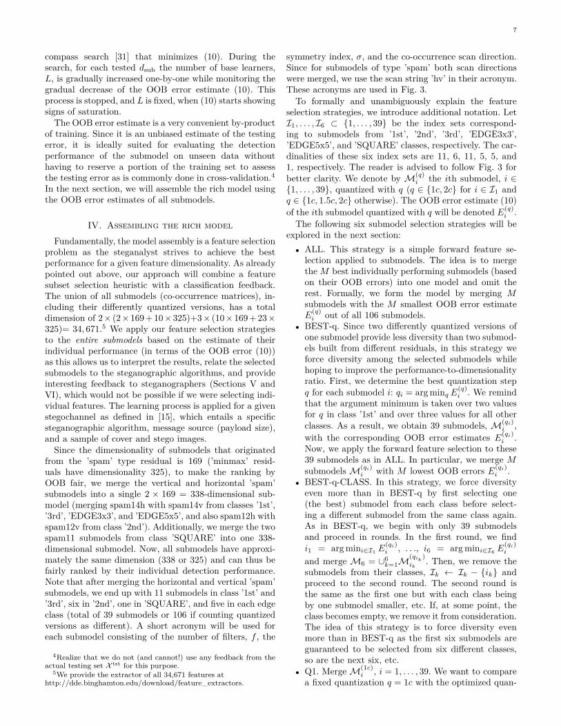
compass search [31] that minimizes (10). During thesearch, for each tested dsub the number of base learners,L, is gradually increased one-by-one while monitoring thegradual decrease of the OOB error estimate (10). Thisprocess is stopped, and L is fixed, when (10) starts showingsigns of saturation.

The OOB error estimate is a very convenient by-productof training. Since it is an unbiased estimate of the testingerror, it is ideally suited for evaluating the detectionperformance of the submodel on unseen data withouthaving to reserve a portion of the training set to assessthe testing error as is commonly done in cross-validation.4In the next section, we will assemble the rich model usingthe OOB error estimates of all submodels.

IV. Assembling the rich model

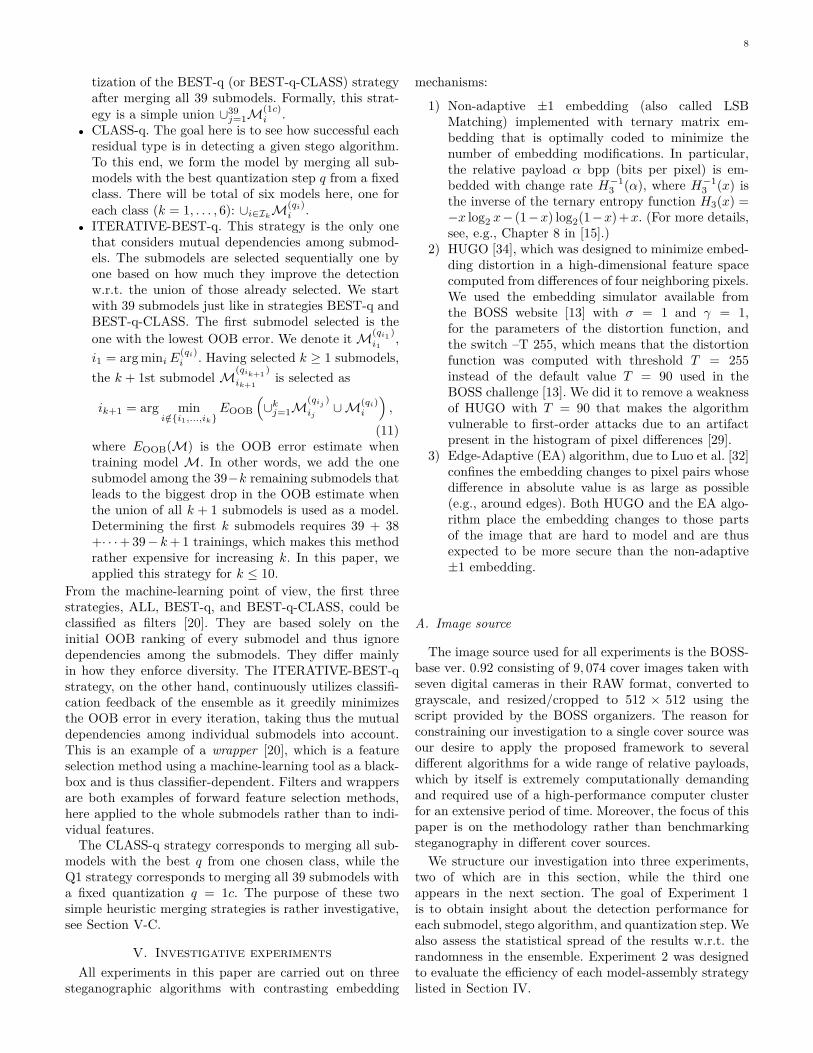
Fundamentally, the model assembly is a feature selectionproblem as the steganalyst strives to achieve the bestperformance for a given feature dimensionality. As alreadypointed out above, our approach will combine a featuresubset selection heuristic with a classification feedback.The union of all submodels (co-occurrence matrices), in-cluding their differently quantized versions, has a totaldimension of 2× (2×169 + 10×325)+3× (10×169 + 23×325)= 34, 671.5 We apply our feature selection strategiesto the entire submodels based on the estimate of theirindividual performance (in terms of the OOB error (10))as this allows us to interpret the results, relate the selectedsubmodels to the steganographic algorithms, and provideinteresting feedback to steganographers (Sections V andVI), which would not be possible if we were selecting indi-vidual features. The learning process is applied for a givenstegochannel as defined in [15], which entails a specificsteganographic algorithm, message source (payload size),and a sample of cover and stego images.

Since the dimensionality of submodels that originatedfrom the ’spam’ type residual is 169 (’minmax’ resid-uals have dimensionality 325), to make the ranking byOOB fair, we merge the vertical and horizontal ’spam’submodels into a single 2 × 169 = 338-dimensional sub-model (merging spam14h with spam14v from classes ’1st’,’3rd’, ’EDGE3x3’, and ’EDGE5x5’, and also spam12h withspam12v from class ’2nd’). Additionally, we merge the twospam11 submodels from class ’SQUARE’ into one 338-dimensional submodel. Now, all submodels have approxi-mately the same dimension (338 or 325) and can thus befairly ranked by their individual detection performance.Note that after merging the horizontal and vertical ’spam’submodels, we end up with 11 submodels in class ’1st’ and’3rd’, six in ’2nd’, one in ’SQUARE’, and five in each edgeclass (total of 39 submodels or 106 if counting quantizedversions as different). A short acronym will be used foreach submodel consisting of the number of filters, f , the

4Realize that we do not (and cannot!) use any feedback from theactual testing set X tst for this purpose.

5We provide the extractor of all 34,671 features athttp://dde.binghamton.edu/download/feature_extractors.

symmetry index, σ, and the co-occurrence scan direction.Since for submodels of type ’spam’ both scan directionswere merged, we use the scan string ’hv’ in their acronym.These acronyms are used in Fig. 3.

To formally and unambiguously explain the featureselection strategies, we introduce additional notation. LetI1, . . . , I6 ⊂ {1, . . . , 39} be the index sets correspond-ing to submodels from ’1st’, ’2nd’, ’3rd’, ’EDGE3x3’,’EDGE5x5’, and ’SQUARE’ classes, respectively. The car-dinalities of these six index sets are 11, 6, 11, 5, 5, and1, respectively. The reader is advised to follow Fig. 3 forbetter clarity. We denote by M(q)

i the ith submodel, i ∈{1, . . . , 39}, quantized with q (q ∈ {1c, 2c} for i ∈ I1 andq ∈ {1c, 1.5c, 2c} otherwise). The OOB error estimate (10)of the ith submodel quantized with q will be denoted E(q)

i .The following six submodel selection strategies will be

explored in the next section:• ALL. This strategy is a simple forward feature se-

lection applied to submodels. The idea is to mergetheM best individually performing submodels (basedon their OOB errors) into one model and omit therest. Formally, we form the model by merging Msubmodels with the M smallest OOB error estimateE

(q)i out of all 106 submodels.

• BEST-q. Since two differently quantized versions ofone submodel provide less diversity than two submod-els built from different residuals, in this strategy weforce diversity among the selected submodels whilehoping to improve the performance-to-dimensionalityratio. First, we determine the best quantization stepq for each submodel i: qi = arg minq E(q)

i . We remindthat the argument minimum is taken over two valuesfor q in class ’1st’ and over three values for all otherclasses. As a result, we obtain 39 submodels, M(qi)

i ,with the corresponding OOB error estimates E(qi)

i .Now, we apply the forward feature selection to these39 submodels as in ALL. In particular, we merge MsubmodelsM(qi)

i with M lowest OOB errors E(qi)i .

• BEST-q-CLASS. In this strategy, we force diversityeven more than in BEST-q by first selecting one(the best) submodel from each class before select-ing a different submodel from the same class again.As in BEST-q, we begin with only 39 submodelsand proceed in rounds. In the first round, we findi1 = arg mini∈I1 E

(qi)i , . . ., i6 = arg mini∈I6 E

(qi)i

and merge M6 = ∪6k=1M

(qik)

ik. Then, we remove the

submodels from their classes, Ik ← Ik − {ik} andproceed to the second round. The second round isthe same as the first one but with each class beingby one submodel smaller, etc. If, at some point, theclass becomes empty, we remove it from consideration.The idea of this strategy is to force diversity evenmore than in BEST-q as the first six submodels areguaranteed to be selected from six different classes,so are the next six, etc.

• Q1. MergeM(1c)i , i = 1, . . . , 39. We want to compare

a fixed quantization q = 1c with the optimized quan-

8

tization of the BEST-q (or BEST-q-CLASS) strategyafter merging all 39 submodels. Formally, this strat-egy is a simple union ∪39

j=1M(1c)i .

• CLASS-q. The goal here is to see how successful eachresidual type is in detecting a given stego algorithm.To this end, we form the model by merging all sub-models with the best quantization step q from a fixedclass. There will be total of six models here, one foreach class (k = 1, . . . , 6): ∪i∈Ik

M(qi)i .

• ITERATIVE-BEST-q. This strategy is the only onethat considers mutual dependencies among submod-els. The submodels are selected sequentially one byone based on how much they improve the detectionw.r.t. the union of those already selected. We startwith 39 submodels just like in strategies BEST-q andBEST-q-CLASS. The first submodel selected is theone with the lowest OOB error. We denote itM(qi1 )

i1,

i1 = arg miniE(qi)i . Having selected k ≥ 1 submodels,

the k + 1st submodelM(qik+1 )ik+1

is selected as

ik+1 = arg mini/∈{i1,...,ik}

EOOB

(∪kj=1M

(qij)

ij∪M(qi)

i

),

(11)where EOOB(M) is the OOB error estimate whentraining model M. In other words, we add the onesubmodel among the 39−k remaining submodels thatleads to the biggest drop in the OOB estimate whenthe union of all k + 1 submodels is used as a model.Determining the first k submodels requires 39 + 38+· · ·+ 39− k+ 1 trainings, which makes this methodrather expensive for increasing k. In this paper, weapplied this strategy for k ≤ 10.

From the machine-learning point of view, the first threestrategies, ALL, BEST-q, and BEST-q-CLASS, could beclassified as filters [20]. They are based solely on theinitial OOB ranking of every submodel and thus ignoredependencies among the submodels. They differ mainlyin how they enforce diversity. The ITERATIVE-BEST-qstrategy, on the other hand, continuously utilizes classifi-cation feedback of the ensemble as it greedily minimizesthe OOB error in every iteration, taking thus the mutualdependencies among individual submodels into account.This is an example of a wrapper [20], which is a featureselection method using a machine-learning tool as a black-box and is thus classifier-dependent. Filters and wrappersare both examples of forward feature selection methods,here applied to the whole submodels rather than to indi-vidual features.The CLASS-q strategy corresponds to merging all sub-

models with the best q from one chosen class, while theQ1 strategy corresponds to merging all 39 submodels witha fixed quantization q = 1c. The purpose of these twosimple heuristic merging strategies is rather investigative,see Section V-C.

V. Investigative experimentsAll experiments in this paper are carried out on three

steganographic algorithms with contrasting embedding

mechanisms:

1) Non-adaptive ±1 embedding (also called LSBMatching) implemented with ternary matrix em-bedding that is optimally coded to minimize thenumber of embedding modifications. In particular,the relative payload α bpp (bits per pixel) is em-bedded with change rate H−1

3 (α), where H−13 (x) is

the inverse of the ternary entropy function H3(x) =−x log2 x− (1−x) log2(1−x)+x. (For more details,see, e.g., Chapter 8 in [15].)

2) HUGO [34], which was designed to minimize embed-ding distortion in a high-dimensional feature spacecomputed from differences of four neighboring pixels.We used the embedding simulator available fromthe BOSS website [13] with σ = 1 and γ = 1,for the parameters of the distortion function, andthe switch –T 255, which means that the distortionfunction was computed with threshold T = 255instead of the default value T = 90 used in theBOSS challenge [13]. We did it to remove a weaknessof HUGO with T = 90 that makes the algorithmvulnerable to first-order attacks due to an artifactpresent in the histogram of pixel differences [29].

3) Edge-Adaptive (EA) algorithm, due to Luo et al. [32]confines the embedding changes to pixel pairs whosedifference in absolute value is as large as possible(e.g., around edges). Both HUGO and the EA algo-rithm place the embedding changes to those partsof the image that are hard to model and are thusexpected to be more secure than the non-adaptive±1 embedding.

A. Image source

The image source used for all experiments is the BOSS-base ver. 0.92 consisting of 9, 074 cover images taken withseven digital cameras in their RAW format, converted tograyscale, and resized/cropped to 512 × 512 using thescript provided by the BOSS organizers. The reason forconstraining our investigation to a single cover source wasour desire to apply the proposed framework to severaldifferent algorithms for a wide range of relative payloads,which by itself is extremely computationally demandingand required use of a high-performance computer clusterfor an extensive period of time. Moreover, the focus of thispaper is on the methodology rather than benchmarkingsteganography in different cover sources.We structure our investigation into three experiments,

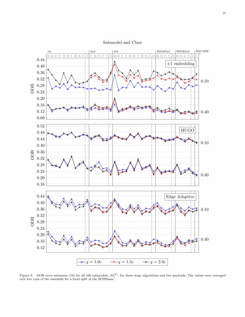
two of which are in this section, while the third oneappears in the next section. The goal of Experiment 1is to obtain insight about the detection performance foreach submodel, stego algorithm, and quantization step. Wealso assess the statistical spread of the results w.r.t. therandomness in the ensemble. Experiment 2 was designedto evaluate the efficiency of each model-assembly strategylisted in Section IV.

9

B. Experiment 1We start by computing the OOB estimates (10) for each

submodel, including its differently quantized versions, foreach stego method and for one small and one large payload(0.1 and 0.4 bpp).6 The intention is to investigate howthe submodel ranking is affected by the stego algorithm,quantization factor, and payload. Note that the ensembleclassifier is built using random structures (randomnessenters the selection of subspaces for base learners and thebootstrap sample formation), which is why we repeatedeach run five times and report the average values of OOBestimates. Table I shows that the variations are in generalrather negligible. They can also be made arbitrarily smallby the user by increasing the number of base learners L.

All results are summarized in Fig. 3 showing the averageOOB error estimates E(q)

i for all i = 1, . . . , 39 and forall values of q. The dashed lines separate the ’spam’ sub-models from submodels of type ’minmax’. The dots wereconnected by a line to enable a faster visual interpretationof the results.

1) Evaluating individual algorithms: By comparing thepatterns for a fixed algorithm, we see that there is a greatdeal of similarity between the performance of submodelsacross payloads even though the actual rankings may bedifferent. Remarkably, ±1 embedding with small payloadshows by far the largest sensitivity to the quantizationfactor than any other combination of algorithms and pay-loads. This effect is caused by the non-adaptive characterof ±1 embedding. For small payloads, the amount ofchanges in edges and textures is so small that detectionessentially relies on smooth parts where the finest quanti-zation discerns the embedding far better in comparisonto other quantizations. On the contrary, both adaptivealgorithms are much less sensitive to the quantization stepbecause small payloads are more concentrated in texturesand edges.

Notice that, for HUGO, submodels built from first-order differences have worse performance than submodelsobtained from third-order differences, which is due to thefact that HUGO approximately preserves statistics amongfirst-order differences; the higher-order differences thusreach “beyond” the model. Also, features of type ’spam’seem to be consistently better than ’minmax’ for thisalgorithm.

The OOB estimates for the EA algorithm exhibit aremarkable similarity for both payloads. This propertycan probably be attributed to the much more selectivecharacter of embedding. While HUGO makes embeddingchanges even in less textured areas albeit with smallerprobability, the EA algorithm limits the embedding onlyto those pairs of adjacent pixels whose difference is above acertain threshold, eliminating a large portion of the imagefrom the embedding process.

2) Universality of submodels: The best individual sub-models for the larger payload and ±1 embedding, HUGO,

6Experiment 1 was carried out on the training set for one fixedsplit of BOSSbase into 8,074 training and 1000 testing images.

Table IMean Absolute Deviation (MAD) of OOB estimates (×10−3)

over five database splits. The table reports the averageand maximal values over all 106 submodels, M(q)

i , for allthree tested stego algorithms and two payloads.

Algorithm ±1 embedding HUGO EAPayload 0.10 0.40 0.10 0.40 0.10 0.40avg. MAD 0.649 0.679 0.656 0.526 0.601 0.484max. MAD 1.640 1.500 2.840 1.220 1.200 0.940

and EA achieve OOB error estimates around 0.1, 0.21, and0.12, indicating that HUGO is by far the best algorithmamong the three. While there exist clear differences amongthe performance of each submodel across algorithms, it isworth noting that certain submodels rank the same w.r.t.each other for all three algorithms, both payloads, and allquantization steps. For example, ’minmax22h’ is alwaysworse than ’minmax22v’ for class ’1st’ as well as ’3rd’. Inother words, it is better to form co-occurrences in the di-rection that is perpendicular to the direction in which thepixel differences are computed. This is most likely becausethe perpendicular scan prevents overlaps of filter supportsand thus utilizes more information among neighboringpixels. The universality of submodels is further supportedby the fact that pair-wise relationships between submodelsare largely invariant to stego method and payload – for40% of all pairs (i, j), i > j, i, j ∈ {1, . . . , 39} thenumerical relationship between errors of modelsM(qi)

i andM(qj)

j does not depend on the algorithm or payload.To further investigate the universality of submodels, in

Fig. 4 we plot for each submodel its OOB error estimateaveraged over all three stego algorithms and five payloads,0.05, 0.1, 0.2, 0.3, and 0.4 bpp. The fact that submodelsfrom ’3rd’ consistently provide lower OOBs than thecorresponding submodels from ’1st’ allowed us to overlapthe results and thus compare both classes visually. Thebest overall submodel is minmax24 in class ’EDGE3x3’.Note that ’h’ versions of submodels built from residualsthat are not hv-symmetrical are almost always worse than’v’ versions as most residuals are defined in Fig. 2 in theirhorizontal orientation. This supports the rule that formingco-occurrence matrices in the direction perpendicular tothe orientation of the kernel support generally leads tobetter detection as the co-occurrence bin utilizes morepixels. Fig. 3 also nicely demonstrates that submodelsbuilt from first-order differences are in general worse thantheir equivalents constructed from third-order differences.Finally, observe that the best submodels are in generalfrom hv-symmetrical non-directional residuals.

C. Experiment 2The purpose of this experiment is to investigate the

efficiency of the submodel-selection strategies explained inSection IV. It is done for a fixed payload of 0.4 bpp for allthree algorithms on the training set for one fixed split ofBOSSbase into 8074 training and 1000 testing images.

1) Evaluation by submodel selection strategies: Fig. 5shows the OOB error estimate as a function of model

10

0.08

0.12

0.16

0.20

0.24

0.28

0.32

0.36

0.40

0.44

OOB

1st 2nd 3rd EDGE3x3 EDGE5x5 SQUARE

22h 22v 24 34 34h 34v 41 48h 48v 54 14hv 21 24h 24v 32 41 12hv 22h 22v 24 34 34h 34v 41 48h 48v 54 14hv 22h 22v 24 41 14hv 22h 22v 24 41 14hv 11

0.10

0.40

Submodel and Class

±1 embedding

0.16

0.20

0.24

0.28

0.32

0.36

0.40

0.44

0.48

0.52

OOB

0.10

0.40

HUGO

0.12

0.16

0.20

0.24

0.28

0.32

0.36

0.40

0.44

OOB

q = 1.0c q = 1.5c q = 2.0c

0.10

0.40

Edge Adaptive

Figure 3. OOB error estimates (10) for all 106 submodels,M(q)i , for three stego algorithms and two payloads. The values were averaged

over five runs of the ensemble for a fixed split of the BOSSbase.

11

22h 22v 24 34 34h 34v 41 48h 48v 54 14hv 21 24h 24v 32 41 12hv22h 22v 24 41 14hv22h 22v 24 41 14hv 110.26

0.28

0.30

0.32

0.34

OOB

error

1st 2nd 3rd EDGE3x3 EDGE5x5 SQUARE

1st

3rd

2nd EDGE3x3

EDGE5x5

SQUARE

Individual submodels

Figure 4. OOB error estimates averaged over all three stego methods and five payloads (0.05, 0.1, . . ., 0.4 bpp). Individual classes are shownin different shades of gray.

dimensionality for all assembly strategies. Diversity-boosting strategies (BEST-q and BEST-q-CLASS) clearlyachieve better results than the simple ALL.As expected, ITERATIVE-BEST-q outperforms all

other strategies but its complexity limited us to mergingonly ten submodels. A little over 3000 features are in gen-eral sufficient to obtain detection accuracy within 0.5−1%of the result when the entire 34,761-dimensional rich modelis used. When all ten submodels are selected using thisstrategy, the best “dependency-unaware” strategy, BEST-q-CLASS, needs roughly double the dimension for compa-rable performance. This seems to suggest that further andprobably substantial improvement of the performance-dimensionality trade-off is likely possible using more so-phisticated feature-selection methods.Overall, the lowest OOB error estimate is indeed ob-

tained when all 106 (dimension 34,671) submodels areused. The gain between usingM = 39 submodels of BEST-q-CLASS (dimensionality 12,753) and all 106 quantizedsubmodels is however rather negligible, indicating a satu-ration of performance.Models assembled from a specific class (CLASS-q) also

provide interesting insight. We obtain another confir-mation that third-order residuals have better detectionaccuracy than first-order residuals across all stego al-gorithms. Remarkably, despite its lower dimension, themodel assembled from class ’2nd’ for HUGO is betterthan class ’1st’. This is not true for the other two al-gorithms and is due to the fact that HUGO preservescomplex statistics computed from first-order differencesamong neighboring pixels. Curiously, while ’EDGE5x5’ isbetter than ’EDGE3x3’ for ±1 embedding and HUGO, theopposite is true for EA. The ’EDGE5x5’ class appears tobe particularly effective against ±1 embedding.Strategy Q1 (the single black cross at dimensionality

12,753 in Fig. 5) does not optimize w.r.t. the quantizationfactor q, and thus it is not surprising that its performanceis generally inferior to the performance of the equally-dimensional BEST-q-CLASS strategy with M = 39

merged submodels. The loss is however rather small (andthere is almost no loss for ±1 embedding). Additionally,Q1 allows the steganalyst to reduce the feature extractiontime roughly to 1/3 as only 39 submodels with q = 1c (outof 106) need to be calculated.

Finally, it is rather interesting that at this payload (0.4bpp) the EA algorithm is less secure than the simple non-adaptive ±1 embedding.

VI. Testing the full frameworkThe purpose of this last experiment is to test the pro-

posed framework in a way it is customary in research workson steganalysis. In particular, for each split of BOSSbaseinto 8,074 training images and 1000 testing images, and foreach payload (0.05, 0.1, 0.2, 0.3, and 0.4 bpp) and stegomethod, we use the BEST-q-CLASS strategy and assemblethe rich model as well as the final steganalyzer using onlythe training set.7 Here, the training set serves the role ofan available sample from the cover source in which secretmessages are to be detected for a known stego method.

We evaluate the performance using the detection erroron the testing set:

PE , minPFA

12(PFA + PMD(PFA)), (12)

as a function of the payload expressed in bpp, where PFAand PMD are the probabilities of false alarm and misseddetection. Fig. 6 shows the median values, P̄E, togetherwith detection errors for the CDF set [30] implementedwith a Gaussian SVM – the state-of-the-art approach be-fore introducing rich models and ensemble classifiers.8 Thefigure contains the results for several models dependingon how many submodels in the BEST-q-CLASS strategyare used; TOPM means that the first M submodels asreported in Fig. 5 were used.

7It is entirely possible that the submodel ranking is slightly differ-ent on each split.

8To save on processing time, we report the results for the CDF setwith a G-SVM for only a single split as the variations over differentsplits are rather small and similar to those of the ensemble.

12

·104

0.07

0.08

0.09

0.10

0.11 SQUARE 2ndEDGE3x3

EDGE5x5

1st

3rd

OOB

±1 embedding

·104

0.130.140.150.160.170.180.190.200.210.22 SQUARE EDGE3x3

EDGE5x5

2nd

1st

3rd

OOB

HUGO

0 1 2 3 4 5 6 7 8 9 10 11 12 13 16 25 35

·104

0.07

0.08

0.09

0.10

0.11

0.12

0.13

0.14

0.15

0.16SQUARE

EDGE5x5

EDGE3x3

2nd 1st

3rd

Dimensionality

OOB

ALL BEST-q BEST-q-CLASS Q1 CLASS-q ITERATIVE-BEST-q

Edge Adaptive

× 103

Figure 5. Performance-to-model dimensionality trade-off for five different submodel selection strategies for three algorithms and a fixedrelative payload of 0.4 bpp. The performance is reported in terms of OOB error estimates. The last three tics on the x axis for strategy ALLare not drawn to scale. The last point corresponds to a model in which all quantized versions of all 106 submodels are merged.

13

0 0.10 0.20 0.30 0.400

0.050.100.150.200.250.300.350.400.450.50

Payload (bpp)

PE

±1 embedding

±1 embedding

payload CDF (G-SVM) TOP 39

(bpp) (single split) MED MAD

0.05 0.3615 0.2740 0.0065

0.10 0.2705 0.1985 0.0057

0.20 0.1890 0.1345 0.0035

0.30 0.1490 0.0968 0.0038

0.40 0.1215 0.0785 0.0035

0 0.10 0.20 0.30 0.400

0.050.100.150.200.250.300.350.400.450.50

Payload (bpp)

PE

HUGO

HUGO

payload CDF (G-SVM) TOP 39

(bpp) (single split) MED MAD

0.05 0.4775 0.4240 0.0045

0.10 0.4540 0.3640 0.0023

0.20 0.3975 0.2658 0.0053

0.30 0.3435 0.1915 0.0033

0.40 0.2750 0.1355 0.0035

0 0.10 0.20 0.30 0.400

0.050.100.150.200.250.300.350.400.450.50

Payload (bpp)

PE

TOP 1 (d ≈ 330) TOP 10 (d ≈ 3286)

TOP 3 (d ≈ 985) TOP 39 (d = 12753)

CDF (d = 1234)

Edge AdaptiveEdge Adaptive

payload CDF (G-SVM) TOP 39

(bpp) (single split) MED MAD

0.05 0.4240 0.3255 0.0028

0.10 0.3555 0.2335 0.0067

0.20 0.2650 0.1445 0.0037

0.30 0.1875 0.0958 0.0038

0.40 0.1390 0.0695 0.0020

CDF . . . dimension d = 1234

TOP 39 . . . dimension d = 12753

Figure 6. Detection error for three stego algorithms as a function of payload for several rich models. P̄E is the median detection errorPE over ten database splits into 8074/1000 training/testing images. The models as well as the classifiers were constructed for each split.The model assembly strategy was BEST-q-CLASS. The tables on the left contain the numerical values and a comparison with a classifierimplemented using Gaussian SVM with the CDF set.

14

A. Evaluation by steganographic methodsThe results confirm that HUGO is by far the best

algorithm of all three capable of hiding the payload 0.05bpp with PE ≈ 0.42. Surprisingly, the security of the EAalgorithm is comparable with that of ±1 embedding forpayloads larger than 0.3 bpp. We observed that at higherpayloads the EA algorithm loses much of its adaptivity andembeds with higher change rate than ±1 embedding dueto its less sophisticated syndrome coding. For smaller pay-loads, the EA algorithm is only slightly more secure than±1 embedding. Overall, the detection of both adaptivestego methods benefits more from the rich model than ±1embedding, which is to be expected and was commentedupon already in Section V-B.

B. Evaluation w.r.t. previous modelsThe proposed detectors provide a substantial improve-

ment in detection accuracy over the 1234-dimensionalCDF set with a Gaussian SVM even when the smallestmodel (TOP1 with dimensionality slightly above 300) isused. This improvement is again much higher for thetwo adaptive stego algorithms. With regards to the morerecent publications on detection of HUGO, we note thatthe results of [19] were reported for HUGO implementedwith T = 90, which introduces artifacts that make thesteganalysis significantly more accurate and thus incompa-rable with the HUGO algorithm run with T = 255 testedhere (see Section V and [29] for more details). Even thoughthe attacks on HUGO reported in [17], [16], [27], [19] didnot explicitly utilize the above-mentioned weakness, they,too are likely affected by the weakness and are thus notdirectly comparable. Having said this, the best resultsof [17] on HUGO (with T = 90) achieved with modeldimensionality of 33,930 can now be matched with ourrich model with dimensionality 30–100 times smaller. Thedecrease in the detection error PE ranges from roughly6% (for payload 0.1 bpp) to about 3% for payload 0.4bpp. For ±1 embedding, the improvement is smaller andranges from 1− 2%.

VII. ConclusionRecent developments in digital media steganalysis

clearly indicate the immense importance of accurate mod-els that are relevant for steganalysis. The accuracy ofsteganalyzers and their ability to detect a wide spectrumof embedding methods in various cover sources stronglydepends on the quality and generality of the cover model.It appears that any substantial progress is only possiblewhen steganalysts incorporate more complex models thatcapture a large number of dependencies among pixels. Thispaper introduces a novel methodology for constructing richmodels of the noise component of digital images, rich in thesense that they consider numerous qualitatively differentrelationships among pixels. The model is assembled fora given sample of the cover source and stego method.Both the model-building and the construction of the fi-nal steganalyzer use ensemble classifiers because of their

good performance that can be achieved with very lowcomplexity. Symmetries of natural images are heavily uti-lized to compactify the model and increase the statisticalsignificance of individual co-occurrence bins forming themodel. Several simple submodel-selection strategies aretested to improve the trade-off between detection accuracyand model dimensionality.

The framework is demonstrated on three stego algo-rithms operating in the spatial domain: ±1 embeddingand two content-adaptive methods – HUGO and an edge-adaptive method by Luo et al. [32]. Ensemble classifierswith the rich model significantly outperform previously-proposed detectors especially for the two adaptive meth-ods as they place embedding changes in hard-to-modelregions of images where the rich model better discerns theembedding changes. Remarkably, the rich model is capableof achieving the same level of statistical detectability withdimensions 30 to 100 times smaller than for the earlyversions of rich models [17], [16], [27].

The rich models are built using the philosophy of max-imizing the diversity of submodels while keeping all theirelements (co-occurrence bins) well populated and thusstatistically significant. This is quite different from themodel used in HUGO, where the authors simply increasedthe truncation threshold to obtain a high-dimensionalmodel. Besides steganalysis, the rich model could be usedfor steganography as well by endowing the model spacewith an appropriate distortion function using, e.g., themethod described in [11]. The authors, however, hypoth-esize that steganographic methods based on minimizingdistortion in a rich model space, such as [10], may no longerbe able to embed large payloads undetectably as it willbecome increasingly harder to preserve a large number ofstatistically significant quantities. This statement stemsfrom an observation made in this paper, namely thatsubmodels built from first-order differences among pixelsare able to detect HUGO relatively reliably despite thefact that its distortion function minimizes perturbationsto joint statistics built from such differences.

We expect that the proposed rich models of the noisecomponent might find applications beyond steganographyand steganalysis in related fields, such as digital forensics,for problems dealing with imaging hardware identification,media integrity, processing history recovery, and authen-tication. A similar framework based on rich models canlikely be adopted for other media types, including audioand video signals.

The steganalyzers and models proposed in this paperconsist of several procedures and modules whose de-sign certainly deserves further investigation and optimiza-tion that might bring further performance improvement.This concerns, for example, the quantizer of the multi-dimensional co-occurrences. Replacing the uniform scalarquantizers with non-uniform or vector quantizers may helpus further improve the performance for a fixed modeldimensionality. Additional boost can likely be obtained byapplying more sophisticated feature selection algorithmsfor choosing the submodels and/or their individual bins.

15

Finally, the local pixel predictors could be parametrizedand optimized w.r.t. a specific stego method and coversource.

As our final remark, we note that one could view themodel-building process independently of the final classi-fier design. It is certainly possible to use the speed andconvenience of the ensemble to assemble the model andthen use it to build a classifier using a different machine-learning tool that may provide a better separation betweenclasses when a highly non-linear boundary exists thatmay not be well captured by the ensemble equipped withlinear base learners. In fact, we observed that featuresbuilt as co-occurrences of neighboring noise residuals oftenlead to non-linear boundaries that are better captured byGaussian SVMs than the ensemble as implemented in thispaper. This has already been observed in our previouswork [17] and is confirmed for our rich model as well.9To demonstrate the potential of this approach, we in-

cluded one more final experiment. We used our best richmodel (best in terms of the OOB error estimate vs. di-mensionality) assembled using the strategy ITERATIVE-BEST-q with ten submodels merged (dimension approx-imately 3300) and trained a G-SVM for all three algo-rithms using the same experimental setup as described inSection VI. This was the largest model we could affordto use with a G-SVM given our computing resources.Calculating the median detection error over ten splits,in Table II we compare the results with the detectionerror of classifiers implemented as ensembles using the12,753-dimensional TOP39 rich model. We only show theresults for the 0.4 bpp payload as carrying out these typesof experiments under our experimental setting (featuredimensionality and training set size) is rather expensivewith a G-SVM. Interestingly, the smaller model with aG-SVM as the final classifier provided our best detectionresults. The improvement is roughly by 0.5–1% over allthree steganographic methods, in terms of the mediantesting error, with a similar level of statistical variabilityover the splits. The running time of a G-SVM classifierwith 3,300-dimensional features, however, was on average30–90 times higher than the running time of the ensembleclassifier with 12,753-dimensional features, as reported inTable III. The measured running times correspond to thefull training and testing, including the parameter-searchprocedures of both types of classifiers. In case of the en-semble, this is the search for the optimal value of dsub, andin case of a G-SVM it is a five-fold cross-validation searchfor the optimal hyper-parameters – the cost parameterC and the kernel width γ. It was carried out on themultiplicative grid GC × Gγ , GC = {10a}, a ∈ {0, . . . , 4},Gγ =

{ 1d · 2

b}, b ∈ {−4, . . . , 3}, where d is the feature

space dimensionality. We used our Matlab implementationof the ensemble classifier10 and the publicly available

9In contrast, in the JPEG domain co-occurrences between quan-tized DCT coefficients appear to react in a more linear fashion toembedding, causing the ensemble to perform equally well as G-SVMs [27], [28].

10available at http://dde.binghamton.edu/download/ensemble

Table IIDetection error PE for three algorithms for payload 0.4

bpp when the ensemble is used with the rich12,753-dimensional TOP39 model and when a G-SVM is

combined with the ∼ 3300-dimensional bestITERATIVE-BEST-q model. The reported numbers are

achieved over ten splits of BOSSbase.

Algorithm Ensemble G-SVMMED MAD MED MAD

±1 Emb. 0.0785 0.0035 0.0683 0.0042HUGO 0.1355 0.0035 0.1310 0.0065EA 0.0695 0.0020 0.0643 0.0030

Table IIIThe average running time (for the training and testing

together) of the experiments in Table II if executed on asingle computer with the AMD Opteron 275 processor

running at 2.2 GHz.

Algorithm Ensemble G-SVM±1 Emb. 1 hr 20 min 4 days 22 hr 37 minHUGO 4 hr 35 min 8 days 15 hr 31 minEA 3 hr 09 min 3 days 23 hr 50 min

package LIBSVM [5] (with manually implemented cross-validation [25]) to conduct the G-SVM experiments.

References

[1] I. Avcibas, M. Kharrazi, N.D. Memon, and B. Sankur. Imagesteganalysis with binary similarity measures. EURASIP Jour-nal on Applied Signal Processing, 17:2749–2757, 2005.

[2] I. Avcibas, N.D. Memon, and B. Sankur. Steganalysis usingimage quality metrics. In E.J. Delp and P.W. Wong, editors,Proceedings SPIE, Electronic Imaging, Security and Water-marking of Multimedia Contents III, volume 4314, pages 523–531, San Jose, CA, January 22–25, 2001.

[3] L. Breiman. Bagging predictors. Machine Learning, 24:123–140,August 1996.

[4] G. Cancelli, G. Doërr, I.J. Cox, and M. Barni. Detection of±1 LSB steganography based on the amplitude of histogramlocal extrema. In Proceedings IEEE, International Conferenceon Image Processing, ICIP 2008, pages 1288–1291, San Diego,CA, October 12–15, 2008.

[5] Chih-Chung Chang and Chih-Jen Lin. LIBSVM: a library forsupport vector machines, 2001. Software available at http://www.csie.ntu.edu.tw/~cjlin/libsvm.

[6] C. Chen and Y.Q. Shi. JPEG image steganalysis utilizing bothintrablock and interblock correlations. In Circuits and Systems,ISCAS 2008. IEEE International Symposium on, pages 3029–3032, May 2008.

[7] C. Chen, Y.Q. Shi, and Wei Su. A machine learning basedscheme for double JPEG compression detection. In 19th In-ternational Conference on Pattern Recognition (ICPR 2008),pages 1–4, Tampa, FL, 2009.

[8] V. Chonev and A.D. Ker. Feature restoration and distor-tion metrics. In N.D. Memon, E.J. Delp, P.W. Wong, andJ. Dittmann, editors, Proceedings SPIE, Electronic Imaging,Security and Forensics of Multimedia XIII, volume 7880, pages0G01–0G14, San Francisco, CA, January 23–26, 2011.

[9] H. Farid and L. Siwei. Detecting hidden messages using higher-order statistics and support vector machines. In F.A.P. Petit-colas, editor, Information Hiding, 5th International Workshop,volume 2578 of Lecture Notes in Computer Science, pages 340–354, Noordwijkerhout, The Netherlands, October 7–9, 2002.Springer-Verlag, New York.

[10] T. Filler and J. Fridrich. Gibbs construction in steganography.IEEE Transactions on Information Forensics and Security,5(4):705–720, 2010.

16

Table IVList of symbols.

X, X̄ cover/stego image C(h)d ,C(v)

d hor./ver. cooc. Ntrn,Ntst no. of train/test pts E(q)i OOB of M(q)

i

I,J index sets R = (Rij) noise residual Bl lth base learner E(L)OOB OOB with L learners

T threshold X̂ij pixel predictor B(l) decision of Bl EOOB(M) OOB with model M

q quant. step c residual order Nbl Bl bootstrap set M(q)

i ith submodel quant. q

truncT truncation f no. of filters Dl lth rand. subspace qi gives smallest OOB for M(q)i

P̄E, PE (median) tst. error σ symmetry index dsub rand.subspace dim. OOB out of bag estimate

H3(x) ternary entropy Nij pixel neighb. L no. of base learners=Cd symmetrized Cd

[11] T. Filler and J. Fridrich. Design of adaptive steganographicschemes for digital images. In N.D. Memon, E.J. Delp, P.W.Wong, and J. Dittmann, editors, Proceedings SPIE, ElectronicImaging, Security and Forensics of Multimedia XIII, volume7880, pages OF 1–14, San Francisco, CA, January 23–26, 2011.

[12] T. Filler, J. Judas, and J. Fridrich. Minimizing additive dis-tortion in steganography using syndrome-trellis codes. IEEETransactions on Information Forensics and Security, 6(3):920–935, 2010.

[13] T. Filler, T. Pevný, and P. Bas. BOSS (Break Our Steganogra-phy System). http://boss.gipsa-lab.grenoble-inp.fr, July 2010.

[14] J. Fridrich. Feature-based steganalysis for JPEG images andits implications for future design of steganographic schemes.In J. Fridrich, editor, Information Hiding, 6th InternationalWorkshop, volume 3200 of Lecture Notes in Computer Science,pages 67–81, Toronto, Canada, May 23–25, 2004. Springer-Verlag, New York.

[15] J. Fridrich. Steganography in Digital Media: Principles, Algo-rithms, and Applications. Cambridge University Press, 2009.

[16] J. Fridrich, J. Kodovský, M. Goljan, and V. Holub. BreakingHUGO – the process discovery. In T. Filler, T. Pevný, A. Ker,and S. Craver, editors, Information Hiding, 13th InternationalWorkshop, volume 6958 of Lecture Notes in Computer Science,pages 85–101, Prague, Czech Republic, May 18–20, 2011.

[17] J. Fridrich, J. Kodovský, M. Goljan, and V. Holub. Steganal-ysis of content-adaptive steganography in spatial domain. InT. Filler, T. Pevný, A. Ker, and S. Craver, editors, InformationHiding, 13th International Workshop, volume 6958 of LectureNotes in Computer Science, pages 102–117, Prague, Czech Re-public, May 18–20, 2011.

[18] M. Goljan, J. Fridrich, and T. Holotyak. New blind steganalysisand its implications. In E.J. Delp and P.W. Wong, editors,Proceedings SPIE, Electronic Imaging, Security, Steganography,and Watermarking of Multimedia Contents VIII, volume 6072,pages 1–13, San Jose, CA, January 16–19, 2006.

[19] G. Gül and F. Kurugollu. A new methodology in steganaly-sis: Breaking highly undetactable steganograpy (HUGO). InT. Filler, T. Pevný, A. Ker, and S. Craver, editors, InformationHiding, 13th International Workshop, volume 6958 of LectureNotes in Computer Science, pages 71–84, Prague, Czech Re-public, May 18–20, 2011.

[20] I. Guyon, S. Gunn, M. Nikravesh, and L. Zadeh, editors. Fea-ture Extraction, Foundations and Applications. Physica-Verlag,Springer, 2006.

[21] J. J. Harmsen and W. A. Pearlman. Steganalysis of additivenoise modelable information hiding. In E.J. Delp and P.W.Wong, editors, Proceedings SPIE, Electronic Imaging, Securityand Watermarking of Multimedia Contents V, volume 5020,pages 131–142, Santa Clara, CA, January 21–24, 2003.

[22] S. Katzenbeisser and F. A. P. Petitcolas, editors. InformationHiding Techniques for Steganography and Digital Watermark-ing. New York: Artech House, 2000.

[23] A.D. Ker and R. Böhme. Revisiting weighted stego-imagesteganalysis. In E.J. Delp and P.W. Wong, editors, ProceedingsSPIE, Electronic Imaging, Security, Forensics, Steganography,and Watermarking of Multimedia Contents X, volume 6819,pages 5 1–5 17, San Jose, CA, January 27–31, 2008.

[24] M. Kirchner and J. Fridrich. On detection of median filteringin images. In Proc. SPIE, Electronic Imaging, Media Forensicsand Security XII, volume 7542, pages 10 1–12, San Jose, CA,January 17–21 2010.

[25] J. Kodovský. On dangers of cross-validation in steganalysis.Technical report, Binghamton University, August 2011.

[26] J. Kodovský and J. Fridrich. On completeness of feature spacesin blind steganalysis. In A.D. Ker, J. Dittmann, and J. Fridrich,editors, Proceedings of the 10th ACM Multimedia & SecurityWorkshop, pages 123–132, Oxford, UK, September 22–23, 2008.

[27] J. Kodovský and J. Fridrich. Steganalysis in high dimensions:Fusing classifiers built on random subspaces. In N.D. Memon,E.J. Delp, P.W. Wong, and J. Dittmann, editors, ProceedingsSPIE, Electronic Imaging, Security and Forensics of MultimediaXIII, volume 7880, pages OL 1–13, San Francisco, CA, January23–26, 2011.

[28] J. Kodovský, J. Fridrich, and V. Holub. Ensemble classifiers forsteganalysis of digital media. IEEE Transactions on Informa-tion Forensics and Security, 2011. Under review.

[29] J. Kodovský, J. Fridrich, and V. Holub. On dangers of overtrain-ing steganography to incomplete cover model. In J. Dittmann,S. Craver, and C. Heitzenrater, editors, Proceedings of the 13thACM Multimedia & Security Workshop, Niagara Falls, NY,September 29–30, 2011.

[30] J. Kodovský, T. Pevný, and J. Fridrich. Modern steganalysiscan detect YASS. In N.D. Memon, E.J. Delp, P.W. Wong, andJ. Dittmann, editors, Proceedings SPIE, Electronic Imaging,Security and Forensics of Multimedia XII, volume 7541, pages02–01–02–11, San Jose, CA, January 17–21, 2010.

[31] T.G. Kolda, R.M. Lewis, and V. Torczon. Optimization bydirect search: New perspectives on some classical and modernmethods. SIAM Review, 45:385–482, 2003.

[32] W. Luo, F. Huang, and J. Huang. Edge adaptive imagesteganography based on LSB matching revisited. IEEE Trans-actions on Information Forensics and Security, 5(2):201–214,June 2010.

[33] T. Pevný, P. Bas, and J. Fridrich. Steganalysis by subtractivepixel adjacency matrix. IEEE Transactions on InformationForensics and Security, 5(2):215–224, June 2010.

[34] T. Pevný, T. Filler, and P. Bas. Using high-dimensional im-age models to perform highly undetectable steganography. InR. Böhme and R. Safavi-Naini, editors, Information Hiding,12th International Workshop, volume 6387 of Lecture Notes inComputer Science, pages 161–177, Calgary, Canada, June 28–30, 2010. Springer-Verlag, New York.

[35] Y. Q. Shi, C. Chen, and W. Chen. A Markov process basedapproach to effective attacking JPEG steganography. In J.L.Camenisch, C.S. Collberg, N.F. Johnson, and P. Sallee, editors,Information Hiding, 8th International Workshop, volume 4437of Lecture Notes in Computer Science, pages 249–264, Alexan-dria, VA, July 10–12, 2006. Springer-Verlag, New York.

[36] K. Sullivan, U. Madhow, S. Chandrasekaran, and B.S. Man-junath. Steganalysis of spread spectrum data hiding exploitingcover memory. In E.J. Delp and P.W.Wong, editors, ProceedingsSPIE, Electronic Imaging, Security, Steganography, and Water-marking of Multimedia Contents VII, volume 5681, pages 38–46,January 16–20,.

[37] D. Upham. Steganographic algorithm JSteg. Software availableat http://zooid.org/~paul/crypto/jsteg.

[38] D. Zou, Y. Q. Shi, W. Su, and G. Xuan. Steganalysis basedon Markov model of thresholded prediction-error image. InProceedings IEEE, International Conference on Multimedia andExpo, pages 1365–1368, Toronto, Canada, July 9–12, 2006.