RICE UNIVERSITY

Modeling Protein Flexibility Using Collective Modes of Motion:

Applications to Drug Design

by

Miguel L. Teodoro

A THESIS SUBMITTED

IN PARTIAL FULFILLMENT OF THE

REQUIREMENTS FOR THE DEGREE

Doctor of Philosophy

APPROVED, THESIS COMMITTEE:

__________________________________

Lydia E. Kavraki, Associate Professor,

Computer Science and Bioengineering

__________________________________

Kevin R. MacKenzie, Assistant Professor,

Biochemistry and Cell Biology

__________________________________

Seiichi Matsuda, Associate Professor

Biochemistry and Cell Biology

__________________________________

John S. Olson, Dorothy and Ralph Looney

Professor, Biochemistry and Cell Biology

__________________________________

George N. Phillips, Jr., Adjunct Professor,

Biochemistry and Cell Biology

HOUSTON, TEXAS

AUGUST, 2003

Abstract

This work shows how to decrease the complexity of modeling flexibility in

proteins by reducing the number of dimensions necessary to model important

macromolecular motions such as the induced fit process. Induced fit occurs during the

binding of a protein to other proteins, nucleic acids or small molecules (ligands) and is

a critical part of protein function. It is now widely accepted that conformational

changes of proteins can affect their ability to bind other molecules and that any progress

in modeling protein motion and flexibility will contribute to the understanding of key

biological functions. However, modeling protein flexibility has proven a very difficult

task. Experimental laboratory methods such as X-ray crystallography produce rather

limited information, while computational methods such as molecular dynamics are too

slow for routine use with large systems. In this work we show how to use the Principal

Component Analysis method, a dimensionality reduction technique, to transform the

original high-dimensional representation of protein motion into a lower dimensional

representation that captures the dominant modes of motions of proteins. For a medium-

sized protein this corresponds to reducing a problem with a few thousand degrees of

freedom to one with less than fifty. Although there is inevitably some loss in accuracy,

we show that we can approximate conformations that have been observed in laboratory

experiments, starting from different initial conformations and working in a drastically

reduced search space. As shown in this work, the accuracy of protein approximations

using this method is similar to the tolerance of current rigid protein docking programs

to structural variations in receptor models.

Acknowledgements

First and foremost, I would like to thank my advisors Dr. George Phillips and

Dr. Lydia Kavraki. Dr. George Phillips provided me with the necessary freedom to

pursue diverse research topics. His invaluable supervision and insight allowed me to

find the perfect project. Dr. Lydia Kavraki has been an extraordinary mentor and friend.

It has been a pleasure and honor to work with her. I thank them, as well as my previous

advisors, Dr. Helena Santos and Dr. António Xavier, for making me a better scientist.

I would like to thank the remaining members of my thesis committee, Dr. Kevin

MacKenzie, Dr. Seiichi Matsuda, and Dr. John Olson for continued guidance and many

helpful suggestions. I am also grateful to all the past and present members of the

Kavraki and Phillips labs for making Rice a fun place to be.

This body of work would not have been possible without financial support from

the PRAXIS XXI program from the Portuguese Foundation for Science and

Technology, the Keck Center for Computational Biology, the Whitaker Foundation, the

National Science Foundation, the Texas Advanced Technology Program, and an Autrey

Fellowship Award from Rice University.

Finally I would like to thank my parents, Luis and Conceição and my wife,

Rosinha, for their love and support of my education and personal growth.

.

Table of Contents

Abstract .......................................................................................................................... ii

Acknowledgements ...................................................................................................... iii

Table of Contents ......................................................................................................... iv

List of Tables .............................................................................................................. viii

List of Figures ............................................................................................................... ix

Chapter 1. Introduction ................................................................................................ 1

1.1. Protein Modeling and Pharmaceutical Drug Design .................................... 1

1.2. Induced Fit Binding ..................................................................................... 2

1.3. The Curse of Dimensionality ....................................................................... 4

1.4. About This Project ....................................................................................... 4

Chapter 2. Background - Protein Flexibility Models in Structure-Based Drug

Design ............................................................................................................................. 5

2.1. Introduction .................................................................................................. 5

2.2. Flexibility Representations .......................................................................... 9

2.2.1. Soft Receptors ............................................................................... 9

2.2.2. Selection of Specific Degrees of Freedom .................................. 12

2.2.3. Multiple Receptor Structures ...................................................... 18

2.2.4. Molecular Simulations ................................................................ 26

2.2.5. Collective Degrees of Freedom ................................................... 32

v

2.4. Summary .................................................................................................... 38

Chapter 3. Tolerance Assessment of Rigid-Protein Docking Methods to Induced

Fit Effects ..................................................................................................................... 39

3.1. Introduction ................................................................................................ 39

3.2. Materials and Methods ............................................................................... 42

3.2.1. Model Systems ............................................................................ 42

3.2.2. Conformational Sampling ........................................................... 43

3.2.3. Autodock ..................................................................................... 47

3.2.4. Dock ............................................................................................ 50

3.3. Results and Discussion ............................................................................... 51

3.4. Summary .................................................................................................... 66

Chapter 4. Calculation of Protein Collective Modes of Motion Using Dimensional

Reduction Methods ..................................................................................................... 68

4.1. Introduction ................................................................................................ 68

4.2. Background ................................................................................................ 70

4.2.1. Dimensional Reduction Methods ................................................ 70

4.2.2. Collective Coordinate Representation of Protein Dynamics....... 73

4.3. Methods ...................................................................................................... 74

4.3.1. Molecular Dynamics Data .......................................................... 74

4.3.2. Experimental Data ....................................................................... 78

4.3.3. Principal Components Analysis and Singular Values

Decomposition ............................................................................. 79

vi

4.4. Results and Discussion ............................................................................... 86

4.4.1. Molecular Dynamics ................................................................... 86

4.4.2. Backbone PCA ............................................................................ 91

4.4.3. Binding Site PCA ...................................................................... 116

4.4.4. All-Atoms PCA ......................................................................... 123

4.4.5. PCA analysis of experimental structures .................................. 126

4.5. Summary .................................................................................................. 137

Chapter 5. Applications of Collective Modes of Motion to Pharmaceutical Drug

Design .......................................................................................................................... 138

5.1. Introduction .............................................................................................. 138

5.2. Generating Docking Targets Using Collective Modes of Motion for

Conformational Sampling ...................................................................... 139

5.3. Identification of Protein Conformational Substates as Docking Targets . 143

5.4. Approximating Molecular Conformations Using Low Dimensional

Representations for Protein Flexibility .................................................. 150

5.5. Summary .................................................................................................. 161

Chapter 6. Conclusions ............................................................................................. 162

Appendix A. Protein Model Systems ....................................................................... 165

A.1. HIV-1 Protease ........................................................................................ 165

A.2. Aldose Reductase .................................................................................... 170

A.3. Dihydrofolate Reductase ......................................................................... 175

A.4. Maltose Binding Protein ......................................................................... 179

vii

Appendix B. HIV-1 Protease Structures ................................................................. 183

Appendix C. Molecular Modeling and Rigid Protein Docking ............................. 197

C.1. Molecular Modeling ................................................................................ 197

C.2. Rigid Protein Docking ............................................................................. 199

References .................................................................................................................. 201

List of Tables

3.1 – Residue numbers included in the binding site RMSD calculation ....................... 45

4.1 – Residue numbers included in the binding site PCA analysis ............................... 84

4.2 – C- RMSD values for different phases of the simulation .................................... 88

B.1 – HIV-1 protease structures used for the PCA analysis ....................................... 181

List of Figures

2.1 – Flexibility representations: soft receptors ......................................................... 11

2.2 – Flexibility representations: selection of specific degrees of freedom ............... 14

2.3 – Flexibility representations: multiple receptor structures ................................... 22

2.4 – Flexibility representations: molecular simulations ........................................... 28

2.5 – Flexibility representations: collective degrees of freedom ............................... 34

3.1 – Conformational sampling of binding site conformations ................................. 46

3.2 – Ligands and degrees of freedom used in docking ............................................. 49

3.3 – a) Autodock docking results for HIV-1 protease ................................................. 54

3.3 – b) Autodock docking results for DHFR ............................................................... 55

3.3 – c) Autodock docking results for aldose reductase ............................................... 56

3.4 – Autodock docking results for HIV-1 protease and DHFR using a very flexible

ligand model ...................................................................................................... 59

3.5 – a) DOCK docking results for HIV-1 protease ..................................................... 60

3.5 – b) DOCK docking results for DHFR ................................................................... 61

3.5 – c) DOCK docking results for aldose reductase .................................................... 62

4.1 – Binding site atoms used for PCA ...................................................................... 84

4.2 – -Carbon RMSD progression for the molecular dynamics simulations ........... 89

4.3 – Eigenvalues results for the backbone PCA analysis ......................................... 92

4.4 – First mode of motion for the backbone of HIV-1 protease ............................... 95

4.5 – Second mode of motion for the backbone of HIV-1 protease .......................... 98

x

4.6 – First mode of motion for the backbone of aldose reductase ............................. 99

4.7 – First mode of motion for the backbone of maltose binding protein ................ 101

4.8 – First mode of motion for the backbone of maltose binding protein ................ 104

4.9 – Second mode of motion for the backbone of maltose binding protein ........... 105

4.10 – Backbone right singular vectors for the MD simulation of HIV-1 protease ... 107

4.11 – Backbone RMSD matrix for the MD simulation of HIV-1 protease .............. 110

4.12 – Backbone right singular vectors for the MD simulation of aldose reductase . 111

4.13 – Backbone RMSD matrix for the MD simulation of aldose reductase ............ 112

4.14 – Backbone right singular vectors for the MD simulation of maltose binding

protein ............................................................................................................. 114

4.15 – Backbone RMSD matrix for the MD simulation of maltose binding protein . 115

4.16 – Eigenvalues results for the binding site PCA analysis .................................... 117

4.17 – Binding site right singular vectors for the MD simulation of HIV-1

protease .......................................................................................................... 120

4.18 – Binding site right singular vectors for the MD simulation of aldose

reductase .......................................................................................................... 121

4.19 – Binding site right singular vectors for the MD simulation of maltose binding

protein ............................................................................................................. 122

4.20 – Eigenvalues results for the all-atoms PCA analysis of HIV-1 protease ......... 125

4.21 – Projection of coordinate vectors of 135 experimental HIV-1 protease structures

on the plane defined by the two dominant eigenvectors of the PCA .............. 128

xi

4.22 - Cumulative inner products from the projection of the molecular dynamics

eigenvectors onto the first three eigenvectors derived from experimental data for

HIV-1 protease ................................................................................................ 132

4.23 – Average deviation from the mean for the right singular vectors of the

experimental and MD data .............................................................................. 135

4.24 – Histogram analysis of the right singular vectors for the experimental and MD

data .................................................................................................................. 136

5.1 – Grid of structure representing protein flexibility ............................................ 141

5.2 – Identification of representative conformations for the binding site of HIV-1

protease ........................................................................................................... 146

5.3 – Identification of representative conformations for the binding site of aldose

reductase .......................................................................................................... 147

5.4 – Identification of representative conformations for the binding site of maltose

binding protein ................................................................................................ 148

5.5 – RMSD between a reference (4HVP) and a target structure (1AID) for an

approximation of the flexibility of the binding site of HIV-1 protease using an

increasing number of collective modes of motion determined by binding site

PCA ................................................................................................................. 152

5.6 – RMSD between a reference (4HVP) and a target structure (1AID) for an

approximation of the flexibility of the binding site of HIV-1 protease using an

increasing number of collective modes of motion determined by all-atoms

PCA ................................................................................................................. 155

xii

5.7 – RMSD between a reference (4HVP) and a target structure (9HVP) for an

approximation of the flexibility of the binding site of HIV-1 protease using an

increasing number of collective modes of motion. determined by binding site

PCA ................................................................................................................. 156

5.8 – RMSD between a reference (1AH4) and a target structure (1AH3) for an

approximation of the flexibility of the binding site of aldose reductase using an

increasing number of collective modes of motion detemined by binding site

PCA ................................................................................................................. 158

5.9 – Approximation of the binding site bound conformation of aldose reductase

using the unbound conformation as a starting point ....................................... 159

A.1 – 3D structure of HIV-1 protease homodimer complexed with an inhibitor .... 166

A.2 – Alternative bound conformations for HIV-1 protease .................................... 169

A.3 – Superposition of the unbound and bound forms of aldose reductase ............. 171

A.4 – Binding site comparison for the unbound and bound forms of aldose

reductase .......................................................................................................... 174

A.5 – Three dimensional structure of DHFR ............................................................ 176

A.6 – Conformational changes during the catalytic cycle of DHFR ........................ 178

A.7 – Three dimensional structure of maltose binding protein ................................ 181

A.8 – Comparison for the unbound and bound forms of maltose binding protein ... 182

1

Chapter 1.

Introduction

1.1. Protein Modeling and Pharmaceutical Drug Design

The three-dimensional structures of protein and nucleic acid molecules are

being determined at increasingly faster rates by X-ray crystallography and Nuclear

Magnetic Resonance. These large molecules play a role in almost all biological

processes either directly, or indirectly by acting as regulators. As a result,

biomacromolecules are key targets for drug design. The rapid generation of quality lead

compounds is a major hurdle in the design of therapeutics, so that accurate automated

procedures would be of tremendous value to the pharmaceutical and other

biotechnology companies. However, designing a drug based on the knowledge of the

target receptor structure as determined by current experimental techniques is a process

prone to error. The two major reasons responsible for failures are imperfect energy

models when scoring potential ligand/receptor complexes (Muegge and Rarey 2001;

Halperin, Ma et al. 2002; Shoichet, McGovern et al. 2002), and the inability of current

methods to predict conformational changes that occur during the binding process not

only for the ligand, but also for the receptor (Carlson 2002; Teodoro and Kavraki

2003). Although the latter problem has been partially solved by incorporating ligand

flexibility in search methods, predicting receptor structural rearrangements is a very

complex problem which has not been solved. The focus of the work reported in this

2

dissertation is to develop a method which can account for receptor conformational

changes that occur during the binding process.

1.2. Induced Fit Binding

Induced fit binding is the process by which both receptor and ligand change

their conformation from the native form in solution to a new minimum energy

conformation which takes into account the interaction of the two molecules. Because

induced fit is a common occurrence in biological systems, in order to be able to

accurately predict docked conformations between a protein and a ligand it is often

necessary to model this effect (Murray, Baxter et al. 1999). Taking into account the

receptor flexibility in structural-based drug design is a natural step in the evolution of

this field and can lead to new classes of drugs which can be effective with lower

dosages and with fewer side effects (Kaul, Cinti et al. 1999). From an industrial point of

view the development of new classes of drugs is also important because it reduces the

probability of intellectual property conflicts with previous patents.

Induced fit conformational changes have been observed experimentally for a

large number of systems. A few examples are thymidylate synthase (Weichsel and

Montfort 1995), chaperonin GroEL (Fenton, Kashi et al. 1994), cyclooxygenase-2

(Luong, Miller et al. 1996), lipoprotein (a) (Fless, Furbee et al. 1996), thrombin

(Banner and Hadvary 1991), cytochrome c peroxidase (Cao, Musah et al. 1998),

phosphofructokinase (Auzat, Gawlita et al. 1995), dihydrofolate reductase (Bystroff and

Kraut 1991), HIV-1 protease (Appelt 1993), aldose reductase, maltose binding protein

3

(Spurlino, Lu et al. 1991; Sharff, Rodseth et al. 1992), and many others. For this study

we decided to use the last four proteins as models systems. For more information on

these proteins and their conformational changes upon binding see Appendix A.

1.3. The Curse of Dimensionality

Current docking programs used commonly in academic and industrial settings

can account for the flexibility of the ligand during induced fit binding. This is carried

out by modeling the degrees of freedom of the ligand explicitly. The degrees of

freedom can be represented by the Cartesian coordinates of every atom in the ligand

molecule. The resulting search space has (3 × N) + 6 degrees of freedom, where N is

the number of atoms in the ligand and the extra 6 six degrees of freedom account for

rotation and translation of the ligand relative to the receptor. The dimensionality of the

problem can be further simplified by considering that bond angles and bond lengths are

fixed. In this case the flexibility of the ligand can be modeled exclusively with torsions

around single bonds. As a result the total number of internal degrees of freedom that

need to be modeled for a traditional ligand is approximately 10 to 20. Although high,

the dimension of the search space is within the capabilities of modern optimization

methods such as genetic algorithms (for more information see Appendix C.).

Including the receptor flexibility in current docking programs by modeling the

protein in the same way as the ligand is currently impossible. Instead of 10 to 20

degrees of freedom, the search space would be composed of hundreds or even

thousands of degrees of freedom. The dimensionality of such a search space is well

4

beyond the capabilities of current computational methods. Given the impossibility of

modeling the receptor using the same methods as the ligand it is imperative to find

alternative docking methods that can be used in structure-based drug design.

1.4. About This Project

In this project we propose a method to reduce the dimensionality of the protein

flexibility space that can be applied to modeling conformational rearrangements such as

induced fit changes upon ligand binding. Unlike other current methods which reduce

the dimensionality of the search space by considering only a few degrees of freedom in

a very limited region of the receptor, our method is able to consider the flexibility of the

protein as a whole. The method described in this work is based on the calculation of a

small set of collective degrees of freedom that account for most of the conformational

variance of the protein.

This work is organized as follows. In Chapter 2 we review current protein

flexibility models which can be used in the context of structure-based drug design. In

Chapter 3 we carry out a quantitative assessment of the tolerance of current rigid-

protein / flexible ligand docking methods to receptor conformational changes. Chapter

4 describes how to obtain a reduced set of collective degrees of freedom that explain

protein flexibility using principal components analysis. The method is applied to three

different model proteins: HIV-1 protease, aldose reductase and maltose binding protein.

Finally in Chapter 5 we explore three different methods of incorporating the

information obtained about protein flexibility in structure-based drug design.

5

Chapter 2.

Background - Protein Flexibility Models

in Structure-Based Drug Design

2.1. Introduction

The ability to predict the bound conformations and interaction energy between

small organic molecules and biological receptors, such as proteins and DNA, is of

extreme physiological and pharmacological importance. Hence, there has been a

considerable effort from both academia and industry to develop computational methods

that can be used to determine the affinity with which a ligand will bind a target

receptor. These methods usually include docking algorithms that compute the three

dimensional structure of the complex as would it be determined experimentally using

X-ray crystallography or Nuclear Magnetic Resonance (NMR) methods. Docking

entails determining not only the identity and three dimensional structure of the bound

ligand, but also how the binding process affects the conformation of the receptor. Here

we review the different receptor flexibility representations that have been proposed to

study receptor conformational changes in the context of structure based drug design.

A central paradigm which was used in the development of the first docking

programs was the lock-and-key model first described by Fischer (Fischer 1894). In this

model the three dimensional structure of the receptor and the ligand complement each

other in the same way that a lock complements a key. According to this model, one

6

could find a good drug candidate by searching a database of small molecules for one

that complemented the three dimensional structure of a given receptor. This rigid

matching was supported by several studies of complexes of proteolytic enzymes with

small protein inhibitors (Blow 1976; Huber and Bode 1978; Hubbard, Campbell et al.

1991) and from the first example of an antibody-protein complex (Amit, Mariuzza et al.

1986). However, subsequent work has confirmed that the lock-and-key model is not the

most correct description for ligand binding. A more accurate view of this process was

first presented by Koshland (Koshland 1958) in the induced fit model. In this model the

three dimensional structure of the ligand and the receptor adapt to each other during the

binding process. It is important to note that not only the structure of the ligand but also

the structure of the receptor changes during the binding process. This occurs because

the introduction of a ligand modifies the chemical and structural environment of the

receptor. As a result, the unbound protein conformational substates, corresponding to

the low energy regions of the protein energy landscape, are likely to change. The

induced fit model is supported by multiple observations in many different proteins

including streptavidin (Weber, Ohlendorf et al. 1989), HIV-1 protease (Wlodawer and

Vondrasek 1998), DHFR (Bystroff and Kraut 1991), aldose reductase (Wilson, Tarle et

al. 1993). The qualitative and quantitative effects of ligand-induced changes in proteins

have been described previously (Betts and Sternberg 1999; Murray, Baxter et al. 1999;

Najmanovich, Kuttner et al. 2000; Zhao, Goodsell et al. 2001; Fradera, Cruz et al.

2002) and explain the ability of a protein to bind multiple drugs with considerably

7

different three dimensional shapes (Wlodawer and Vondrasek 1998; Vazquez-Laslop,

Zheleznova et al. 2000).

A more modern, but not contradictory, model for protein/ligand binding

considers the binding process as a selection of a particular receptor conformation from

an ensemble of metastable states (Ma, Kumar et al. 1999; Ma, Wolfson et al. 2001;

Bursavich and Rich 2002; Ma, Shatsky et al. 2002). The protein exists as a family of

similar conformations in a hierarchical energy landscape (Verkhivker, Bouzida et al.

2002). Successful binding shifts the dynamic population equilibrium in favor of the

bound receptor conformation. This model of ligand binding suggests that for the design

of novel inhibitors we may need to explore receptor conformations beyond the narrow

scope of the conformational ensemble presently determined using experimental

methods. This is important for drug design because it clearly illustrates the need to

consider protein flexibility and the existence of multiple receptor conformations. It also

provides a justification for higher affinity inhibitors that do not mimic substrates at their

transition state. Additionally, if a protein exists in a population of states as discussed in

(Carlson and McCammon 2000; Ma, Shatsky et al. 2002) then one could either design a

moderate affinity ligand for a highly populated conformer (lower energy) or a high

affinity ligand for a less populated conformer (higher energy).

Although it has been clearly established that a protein is able to undergo

conformational changes during the binding process, most docking studies consider the

protein as a rigid structure. The reason for this crude approximation is the extraordinary

increase in computational complexity that is required to include the degrees of freedom

8

of a protein in a modeling study. Pioneer efforts in the docking area (Holtje and Kier

1974; Kier and Aldrich 1974) were limited not only in methodology but also in

computational capability. In the 1980s Kuntz and coworkers developed the program

DOCK (Kuntz, Blaney et al. 1982) which made structure-based drug design a staple of

current pharmaceutical research methods. Currently available docking software

includes improved versions of the original DOCK(Ewing and Kuntz 1997), FlexX

(Rarey, Kramer et al. 1996) and Autodock (Morris, Goodsell et al. 1998), among many

others, to computationally predict the spatial conformation and affinity of bound

complexes between a flexible ligand and a rigid receptor. These programs use different

search methods and scoring functions. A review of these is beyond the scope of this

chapter. For recent reviews on docking methods and scoring functions see (Gane and

Dean 2000; Klebe 2000; Muegge and Rarey 2001; Halperin, Ma et al. 2002; Shoichet,

McGovern et al. 2002).

The three dimensional conformation of a molecule can be represented by the

values corresponding to its degrees of freedom. These are usually the Cartesian

coordinates of its individual atoms or alternatively the values for its internal degrees of

freedom. The latter are bond lengths, bond angles and dihedral angles (i.e., torsions

around single bonds). A common approximation when modeling organic molecules is

to consider that bond lengths and bond angles are constant and only dihedral angles are

free to change. Even when using this approximation, a protein can have thousands of

degrees of freedom whereas a small organic molecule can be usually modeled using

only five to twenty degrees of freedom. In the last decade, with the advent of improved

9

computational capabilities, researchers have been trying to solve the high dimensional

problem of modeling protein flexibility in docking applications. The effect of protein

flexibility on structure based drug design has been reviewed by Carlson et al. (Carlson

and McCammon 2000; Carlson 2002; Carlson 2002).

There is currently no computationally efficient docking method that is able to

screen a large database of potential ligands against a target receptor while considering

the full flexibility of both ligand and receptor. In order for this process to become

efficient, it is necessary to find a representation for protein flexibility that avoids the

direct search of a solution space comprised of thousands of degrees of freedom. Here

we review the different representations that have been used to incorporate protein

flexibility in the modeling of protein/ligand interactions. A common theme behind all

these approaches is that the accuracy of the results is usually directly proportional to the

computational complexity of the representation. We tried to group the different types of

flexibility representations models into categories that illustrate some of the key ideas

that have been presented in the literature in recent years. However it is important to

note that the boundaries between these categories are not rigid and in fact several of the

publications referenced below could easily fall in more than one category.

2.2. Flexibility Representations

2.2.1. Soft Receptors

Perhaps the simplest solution to represent some degree of receptor flexibility in

docking applications is the use of soft receptors. Soft receptors can be easily generated

10

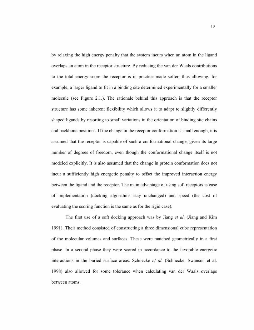
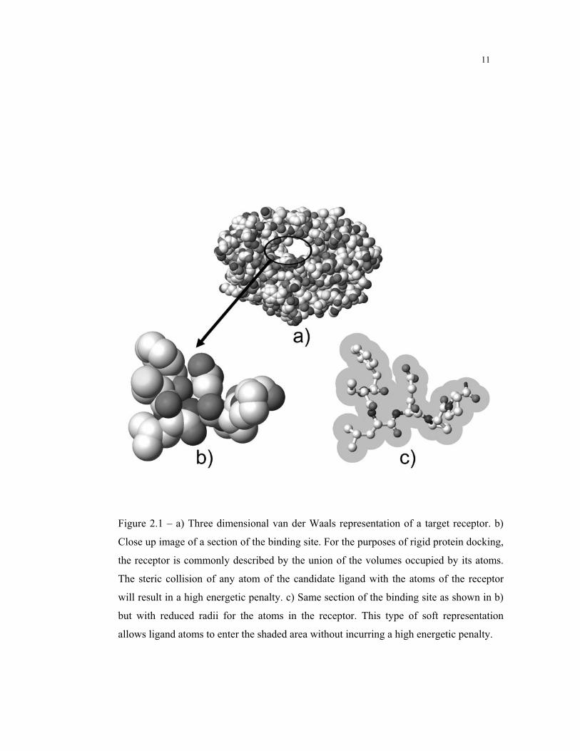
by relaxing the high energy penalty that the system incurs when an atom in the ligand

overlaps an atom in the receptor structure. By reducing the van der Waals contributions

to the total energy score the receptor is in practice made softer, thus allowing, for

example, a larger ligand to fit in a binding site determined experimentally for a smaller

molecule (see Figure 2.1.). The rationale behind this approach is that the receptor

structure has some inherent flexibility which allows it to adapt to slightly differently

shaped ligands by resorting to small variations in the orientation of binding site chains

and backbone positions. If the change in the receptor conformation is small enough, it is

assumed that the receptor is capable of such a conformational change, given its large

number of degrees of freedom, even though the conformational change itself is not

modeled explicitly. It is also assumed that the change in protein conformation does not

incur a sufficiently high energetic penalty to offset the improved interaction energy

between the ligand and the receptor. The main advantage of using soft receptors is ease

of implementation (docking algorithms stay unchanged) and speed (the cost of

evaluating the scoring function is the same as for the rigid case).

The first use of a soft docking approach was by Jiang et al. (Jiang and Kim

1991). Their method consisted of constructing a three dimensional cube representation

of the molecular volumes and surfaces. These were matched geometrically in a first

phase. In a second phase they were scored in accordance to the favorable energetic

interactions in the buried surface areas. Schnecke et al. (Schnecke, Swanson et al.

1998) also allowed for some tolerance when calculating van der Waals overlaps

between atoms.

11

Figure 2.1 – a) Three dimensional van der Waals representation of a target receptor. b)

Close up image of a section of the binding site. For the purposes of rigid protein docking,

the receptor is commonly described by the union of the volumes occupied by its atoms.

The steric collision of any atom of the candidate ligand with the atoms of the receptor

will result in a high energetic penalty. c) Same section of the binding site as shown in b)

but with reduced radii for the atoms in the receptor. This type of soft representation

allows ligand atoms to enter the shaded area without incurring a high energetic penalty.

12

Another use of soft docking models is to improve convergence during energy

minimization of the complex by avoiding local minima. Apostolakis et al. (Apostolakis,

Pluckthun et al. 1998) developed a docking approach that is based on a combination of

Monte Carlo and shifted nonbonded interactions minimization. In the initial stages of

the conformational search the ligand is allowed to overlap with the receptor and

nonbonded energy terms are modified to avoid high energy gradients. During the

course of the minimization the interactions are then gradually restored to their original

values simulating a ligand that is gradually exposed to the field of the receptor. This

allows initial ligand/receptor conformations, which due to steric clashes would result in

a very high energy penalty, to slowly adapt to each other in a complementary

conformation without overlaps. One potential pitfall of this approach is the possibility

that the ligand may become interlocked with the protein, leading to failure of the

docking procedure to arrive at the minimal energy configuration.

Although the use of soft receptors presents a number of advantages such as ease

of implementation and computation speed, it also makes use of conformational and

energetic assumptions that are difficult to verify. This can easily result in errors,

especially if the soft region is made excessively large to account for larger

conformational changes on the part of the receptor.

2.2.2. Selection of Specific Degrees of Freedom

In order to reduce the complexity of modeling the very large dimensional space

representing the full flexibility of the protein, it is possible to obtain an approximate

solution by selecting only a few degrees of freedom to model explicitly. The degrees of

13

freedom chosen usually correspond to rotations around single bonds (see Figure 2.2).

The reason for this choice is that these degrees of freedom are usually considered the

natural degrees of freedom in molecules. Rotations around bonds lead to deviations

from ideal geometry that result in a small energy penalty when compared to deviations

from ideality in bond lengths and bond angles. This assumption is in good agreement

with current modeling force fields such as CHARMM (MacKerell, Bashford et al.

1998) and AMBER (Cornell, Cieplak et al. 1995). Choosing which torsional degrees of

freedom to model is usually the most difficult part of this method because it requires a

considerable amount of a priori knowledge of alternative binding modes for a given

receptor. This knowledge is usually a result of the availability of experimental

structures obtained under different conditions or using different ligands. If multiple

experimental structures are not available some insight can be obtained from simulation

methods such as Monte Carlo (MC) or molecular dynamics (MD). The torsions chosen

are usually rotations of aminoacid side chains in the binding site of the receptor protein.

It is also common to further reduce the search space by using rotamer libraries for the

aminoacid side chains (Tuffery, Etchebest et al. 1991; Lovell, Word et al. 2000;

Dunbrack 2002).

14

Figure 2.2 – Stick representation of the same binding site section as shown in Figure 2.1.

In order to approximate the flexibility of the receptor it is possible to carefully select a

few degrees of freedom. These are usually select torsional angles of sidechains in the

binding site that have been determined to be critical in the induced fit effect for a specific

receptor. In this example the selected torsional angles are represented by arrows.

15

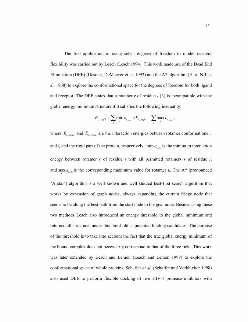
The first application of using select degrees of freedom to model receptor

flexibility was carried out by Leach (Leach 1994). This work made use of the Dead End

Elimination (DEE) (Desmet, DeMaeyer et al. 1992) and the A* algorithm (Hart, N.J. et

al. 1968) to explore the conformational space for the degrees of freedom for both ligand

and receptor. The DEE states that a rotamer r of residue i (ir) is incompatible with the

global energy minimum structure if it satisfies the following inequality:

j

jis

rigidi

j

jis

rigidi sttsrrEE ,,,, maxmin ,

where rigidirE , and rigidit

E , are the interaction energies between rotamer conformations ir

and it and the rigid part of the protein, respectively, sr ji

s,min is the minimum interaction

energy between rotamer r of residue i with all permitted rotamers s of residue j,

andst ji

s,max is the corresponding maximum value for rotamer it. The A* (pronounced

"A star") algorithm is a well known and well studied best-first search algorithm that

works by expansion of graph nodes, always expanding the current fringe node that

seems to be along the best path from the start node to the goal node. Besides using these

two methods Leach also introduced an energy threshold to the global minimum and

returned all structures under this threshold as potential binding candidates. The purpose

of the threshold is to take into account the fact that the true global energy minimum of

the bound complex does not necessarily correspond to that of the force field. This work

was later extended by Leach and Lemon (Leach and Lemon 1998) to explore the

conformational space of whole proteins. Schaffer et al. (Schaffer and Verkhivker 1998)

also used DEE to perform flexible docking of two HIV-1 protease inhibitors with

16

mutants of this protein. The DEE algorithm was applied using a rotamer library to

perform discrete optimization of all possible combinations of side chain conformations

in the binding site. The best solutions were later optimized in conjunction with the

ligand using a Monte Carlo simulated annealing technique. This two step method leads

to a solution that is not restricted to the dihedral values present in the rotamer library

and is also of lower energy. More recently Althaus et al. (Althaus, Kohlbacher et al.

2002) also used two alternative combinatorial optimization methods to solve the side

chain conformation problem. The first method consists of a heuristic multi-greedy

approach, which is faster but does not necessarily produce an optimal solution. The

second method is able to find the global minimum energy conformation and is based on

a branch-and-cut algorithm and integer linear programming.

In the program GOLD, Jones et al. (Jones, Willett et al. 1997) use a genetic

algorithm (GA) to dock a flexible ligand to a semi-flexible protein. GAs are an

optimization method that derive their behavior from a metaphor of the process of

evolution. A solution to a problem is encoded in a chromosome and a fitness score is

assigned to it based on the relative merit of the solution. A population of chromosomes

then goes through a process of evolution in which only the fittest solutions “survive”.

This program takes into account not only the position and conformation of the ligand

but also the hydrogen bonding network in the binding site. This was achieved by

encoding orientation information for donor hydrogen atoms and acceptors in the GA

chromosome. This type of conformational information is very important because if the

starting point for a docking study is a rigid crystallographic structure, the orientations of

17

hydroxyl groups will be undetermined. Being able to model these orientations explicitly

removes any bias that might result from positioning hydroxyl groups based upon a

known ligand. One limitation of this work is that the binding site still remains

essentially rigid because protein conformational changes are limited to a few terminal

bonds. This program performed very well for hydrophilic ligands but encountered some

difficulties when trying to dock hydrophobic ligands due to the reduced contribution of

hydrogen bonding to the binding process.

In SPECITOPE Schnecke et al. (Schnecke, Swanson et al. 1998) also make use

of side chain rotations in the late stages of docking to remove steric overlaps between

the protein side chains and the ligand. If an overlap clash is detected, the program

attempts to remove it by rotating the side chain through the minimal angle that resolves

the clash. The single bond closest to the bumping atoms in the side chain is used first to

resolve the overlap. If a bump free conformation cannot be generated with this rotation,

the next rotatable bond closer to the ligand backbone is rotated. This procedure will

miss potential combinations of side chain conformations that do not overlap with the

ligand and is not capable of finding the minimum energy conformation. Nevertheless, it

will successfully resolve many cases of overlap.

Anderson et al. (Anderson, O'Neil et al. 2001) introduced the algorithm

SOFTSPOTS that addresses the problem of knowing which rotational degrees of

freedom should be selected to represent receptor flexibility. Using a single protein

structure, this algorithm is capable of identifying regions of high flexibility. The results

were combined with a second algorithm named PLASTIC that provides a collection of

18

possible conformations based on rotamer libraries effectively reducing the bias caused

by structures of proteins co-crystallized with inhibitors. More recently, Kayrys et al.

(Kairys and Gilson 2002) have improved the Mining Minima optimizer method, first

described by David et al. (David, Luo et al. 2001), to include select side chain degrees

of freedom in the docking simulation of several proteins and ligands.

A common theme among the work described in this section is that receptor side

chain conformations are modeled using torsional degrees of freedom. In order to make

the calculation of interaction energies more efficient it would be desirable to work with

a force field that is also described in terms of internal coordinates to avoid repeated

conversion between two coordinate systems. Use of internal coordinate force fields also

leads to more efficient convergence of energy optimizations. Abagyan et al. described a

method to carry out flexible protein-ligand docking by global energy optimization in

internal coordinates (Totrov and Abagyan 1997) and more recently described a method

to accurately "project" a Cartesian force field onto an internal coordinate molecular

model with fixed-bond geometry (Katritch, Totrov et al. 2003).

2.2.3. Multiple Receptor Structures

One possible way to represent a flexible receptor for drug design applications is

the use of multiple static receptor structures (see Figure 2.3). This concept is supported

by the currently accepted model that proteins in solution do not exist in a single

minimum energy static conformation but are in fact constantly jumping between low

energy conformational substates (Noguti and Go 1989; Frauenfelder, Sligar et al. 1991;

Andrews, Romo et al. 1998; Kitao, Hayward et al. 1998). In this way the best

19

description for a protein structure is that of a conformational ensemble (Bursavich and

Rich 2002; Rich, Bursavich et al. 2002) of slightly different protein structures

coexisting in a low energy region of the potential energy surface. Moreover the binding

process can be thought of as not exactly an induced fit model as first described by

Koshland (Koshland 1958) but more like a selection of a particular substate from the

conformational ensemble that best complements the shape of a specific ligand (Ma,

Kumar et al. 1999).

The use of multiple static conformations for docking gives rise to two critical

questions. The first question is “How can we obtain a representative subset of the

conformational ensemble typical of a given receptor?” Currently, the three dimensional

structure of macromolecules can be determined experimentally using X-ray

crystallography or NMR, or generated via computational methods such as Monte Carlo

or molecular dynamics simulations. Simulations typically use as a starting point a

structure determined by one of the experimental methods. Ideally we would like to use

a sampling that provides the most extensive coverage of the structure space.

Comparisons between traditional molecular simulations and experimental techniques

(Clarage, Romo et al. 1995; Philippopoulos and Lim 1999) indicate that X-ray

crystallography and NMR structures seem to provide better coverage. However this

balance can potentially change due to advances in computational methods (Karplus and

McCammon 2002). Another limitation in choosing data sources is availability.

Although experimental data is preferable, the monetary and time cost of determining

multiple structures experimentally is significantly higher than obtaining the same

20

amount of data computationally. The second critical question is “What is the best way

of combining this large amount of structural information for a docking study?”. This

question also remains open. Current approaches use diverse ways of combining

multiple structures as discussed below.

The first use of multiple structures for a drug design applications was by Pang

and Kozikowski (Pang and Kozikowski 1994) to study the binding of huperzine A

(HA) to acetylcholinesterase (AChE). In this study the authors ran a short molecular

dynamics simulation (40 ps) of AChE from which they extracted 69 conformations that

were docked to HA using rigid docking. This study successfully predicted that HA

binds to the bottom of the binding cavity of AChE (the gorge). More recently, other

studies (Kua, Zhang et al. 2002; Lin, Perryman et al. 2002) have exploited similar

approaches but used a larger number of structures, longer molecular dynamics

sampling, and more accurate simulation conditions. Instead of resorting to

computational methods to derive structural data Knegtel et al. (Knegtel, Kuntz et al.

1997) used a family of structures from an NMR structural determination or, as an

alternative, several crystal structures of the same protein system. In that study the

authors combined the different structures into a single interaction energy grid to be used

for rigid receptor docking by the DOCK program. Interaction energy grids are

calculated by placing a probe atom at discrete points in the space around a target

protein and assigning to the grid point the value of the interaction energy between the

probe and protein. This grid is then utilized as a fast lookup table for interaction energy

calculations, effectively reducing the cost of computation from quadratic to linear. The

21

averaged grids were constructed using energy-weighted and geometry-weighted

averaging methods. The main limitation of these averaging approaches is that they can

lead to loss of geometric accuracy. The binding energies computed from the composite

grid are also less favorable than for individual grids for each protein in the ensemble. In

the case of geometry-weighted averaging, the binding site can become too permissive

in terms of the size of the ligand that it can accommodate. Sudbeck et al. (Sudbeck,

Mao et al. 1998) superimposed the crystal structures of nine inhibitor complexes of

HIV reverse transcriptase to generate a composite binding site that summarized its

unique critical features. The overlaid coordinates of the nine different inhibitors were

used to generate a combined molecular surface defining an enlarged binding pocket that

represented the plasticity of the receptor. The combined binding pocket was used to

verify the results obtained from the docking of small molecules to a single structure of

reverse transcriptase through a conjugate gradient minimization method for the ligand

and all residues within 5 Å. This study resulted in the development of two new

inhibitors. Multiple crystal structures of HIV-1 protease were also used by Bouzida et

al. (Bouzida, Rejto et al. 1999) to account for receptor flexibility. Broughton et al.

(Broughton 2000) used different conformation snapshots from a short molecular

dynamics simulation of dihydrofolate reductase to generate interactions grids that were

also combined into a single grid by means of a weighted average method. Before the

calculation of the grids, the structures were superimposed using the bound inhibitors as

a reference.

22

Figure 2.3 – Superposition of multiple conformers of the same binding site section as

shown in Figure 2.1. As an alternative to considering the target protein as a single three

dimensional structure, it is possible to combine information from multiple protein

conformations in a drug design effort. These can be either considered individually as

rigid representatives of the conformational ensemble or can be combined into a single

representation that preserves the most relevant structural information.

23

As mentioned earlier one of the methods of combining multiple receptor

structures is to create an average grid for the protein/ligand interaction potential

(Knegtel, Kuntz et al. 1997). Osterberg et al. (Osterberg, Morris et al. 2002) analyzed

this problem in depth by using HIV-1 protease as a model system and comparing four

different grid averaging methods. The fist two naïve methods consisted of a mean grid

that takes a simple point-by-point average across all the grids, and a minimum grid that

takes the minimum value across all the grids. Both methods performed poorly. The

third approach is similar to that described by Knegtel et al. (Knegtel, Kuntz et al. 1997)

and consists of a weighted averaging scheme. In this case if one or more of the grids

contain a favorable, negative value, their weights will dominate the average. On the

other hand, if all the grids contain unfavorable positive values, all will have identical

small weights resulting in an unfavorable region representing all grids. The fourth

averaging scheme is similar to the previous one but uses a Boltzmann assumption to

calculate the weight based on the interaction energy. The last two averaging schemes

were able to efficiently represent multiple structures in a single grid and the docking

results were satisfactory. However, as the authors point, out this method for

incorporation of conformational flexibility can introduce potentially dangerous artifacts

such as positive interaction regions for mutually exclusive solutions.

A different way of considering protein flexibility as represented in interaction

grids for multiple static structures is GRID/CPCA (Consensus Principal Component

Analysis). This method, introduced by Kastenholz et al. (Kastenholz, Pastor et al. 2000)

in the study of serine proteases, is an extension of GRID/PCA (Pastor and Cruciani

24

1995), and can be used to identify selectivity features for a receptor. One of the main

advantages of this method over its predecessor is that it allows the inclusion of more

that two structures in the PCA calculation. Moreover, when several structures are used,

it allows for some averaging of individual structures, reducing differences that might be

present due to experimental variations but are not relevant to the specificity features of

the receptors.

In the program FlexE, Claussen et al. (Claussen, Buning et al. 2001) introduced

a new method of combining multiple receptor structures to represent a flexible binding

site. The algorithm starts by superimposing the set of conformations available for a

given receptor and merging similar parts of the structures. Dissimilar substructures are

treated as independent alternatives and FlexE selects the combination of substructures

that best complements conformations of the ligand with respect to the scoring function.

In practice, this results in the generation of alternative receptor conformations that were

not present in the initial set but may constitute valid docking targets.

More recently Moreno and León (Moreno and Leon 2002) introduced a new

receptor representation that allows the use of an ensemble of protein structures as input

to DOCK instead of a single rigid structure. In this approach, an ensemble of

protein/inhibitor complex structures is used to construct a set of templates of attached

points (one for each type of amino acid) located in positions suitable for interactions

with ligand atoms. The combination of templates gives a description of a flexible

binding site. The authors propose the method of attached points as an alternative to

25

SPHGEN (Bolin, Filman et al. 1982; DesJarlais, Sheridan et al. 1988) or SURFSPH

(Oshiro and Kuntz 1998) to generate a binding site descriptor.

Multiple protein structures can be used not only to generate flexible receptor

representations for docking purposes, but also to generate pharmacophores. A

pharmacophore is a template for the desired ligand. The pharmacophore is represented

by a set of features that an effective ligand should possess and a set of spatial

constraints among the features. The features can be specific atoms, positive or negative

charges, hydrophobic or hydrophilic centers, hydrogen bond donors or acceptors, and

others. The spatial arrangement of the features represents the relative 3D placements of

these features in the docked conformation of the ligand. Carlson et al. introduced the

concept of a dynamic pharmacophore by combining sets of structures derived by either

X-ray crystallography (Carlson, Masukawa et al. 1999) or snapshots of a molecular

dynamics simulation (Carlson, Masukawa et al. 2000). Potential sites of interest in the

receptor binding site are determined by running a multi-unit Monte Carlo minimization

using probe molecules for the different features of interest. The results of these

simulations for each conformer are then overlaid. This procedure reveals conserved

binding regions that are highly occupied during the molecular dynamics simulation

despite the flexibility of the receptor. The conserved features define the dynamic

pharmacophore. Studies similar to dynamic pharmacophore identification were

performed by Stultz and Karplus (Stultz and Karplus 1999) using a combination of the

Multiple Copy Simultaneous Search (MCSS) and Locally Enhanced Sampling (LES)

methods (Roitberg and Elber 1991). Their protocol uses quenched molecular dynamics

26

to identify energetically favorable positions and orientations of small functional groups

in a flexible binding site. In this method multiple copies of the functional groups are

distributed in the binding site and quenched to find energy minima. These functional

groups can later be used as building blocks for larger ligands.

One of the main advantages of using multiple structures instead of using a

selection of degrees of freedom to represent protein flexibility is that the flexible region

is not limited to a specific small region of the protein. Multiple structures allow the

consideration of the full flexibility of the protein without the exponential blow up in

terms of computational cost that would derive from including all the degrees of

freedom of the protein. On the other hand, flexibility is modeled implicitly and as such

only a small fraction of the conformational space of the receptor is represented. In

addition, the method by which the multiple receptor structures are combined has a

drastic influence on the possible results of the docking computation.

2.2.4. Molecular Simulations

To simulate the binding process with as much detail as possible and avoid some

of the limitations of previous flexibility models one can use force field based atomistic

simulation methods such as Monte Carlo or molecular dynamics (see Figure 2.4.).

Whereas molecular dynamics applies the laws of classical mechanics to compute the

motion of the particles in a molecular system, Monte Carlo methods are so called

because they are based on a random sampling of the conformational space. The main

advantage of Monte Carlo or molecular dynamics flexibility representations in docking

studies is that they are very accurate and can model explicitly all degrees of freedom of

27

the system including the solvent if necessary. Unfortunately, the high level of accuracy

in the modeling process comes with a prohibitive computational cost. For example, in

the case of molecular dynamics, state of the art protein simulations can only simulate

periods ranging from 10 to 100 ns, even when using large parallel computers or

clusters. Given that diffusion and binding of ligands takes place over a longer time

span, it is clear that these simulations techniques cannot be used as a general method to

screen large databases of compounds in the near future. It is however possible to carry

out approximations that reduce the computational expense and lead to insights that

would be impossible to gain using less flexible receptor representations. The cost of

carrying out the computational approximations is usually a loss in accuracy.

28

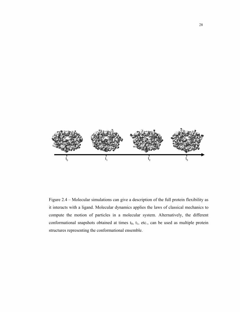
Figure 2.4 – Molecular simulations can give a description of the full protein flexibility as

it interacts with a ligand. Molecular dynamics applies the laws of classical mechanics to

compute the motion of particles in a molecular system. Alternatively, the different

conformational snapshots obtained at times t0, t1, etc., can be used as multiple protein

structures representing the conformational ensemble.

29

In order to address the time sampling limitations of traditional molecular

dynamics Di Nola et al. (Di Nola, Roccatano et al. 1994) used a modified temperature

coupling scheme to perform the docking of phosphocholine onto immunoglobulin

McPC603. Instead of coupling the whole system to the same temperature bath, Di Nola

used a regular coupling temperature to the internal degrees of freedom of the ligand and

a very high temperature (1300-1700 K) for the translational modes. In practice, this

allows the ligand to sample the surface of a protein receptor much faster and without

disturbing internal motions. This method was extended later by Mangoni et al.

(Mangoni, Roccatano et al. 1999) to also include the flexibility of the receptor, which

was also coupled to the lower temperature bath (300 K). In order to further reduce the

computational cost of the simulation, the protein simulation was restricted to a sphere

of 20 Å around the chain oxygen of the phosphocholine molecule in the

crystallographic position. The remaining part of the protein was kept rigid. The same

approach of restricting the full molecular simulation to the vicinity of the binding site

was used by Luty et al. (Luty, Wasserman et al. 1995) to simulate the docking of

benzamidine to trypsin and by Wasserman et al. (Wasserman and Hodge 1996) to

simulate the docking of L-leucine hydroxamic acid to thermolysin. Given and Gilson

(Given and Gilson 1998) also restricted flexibility to the binding site area of HIV-1

protease within the context of a hierarchical docking protocol. In this method

conformations are evolved in stages, with the lowest energy conformations from one

stage serving as starting points for the next. The focus of this study was not to develop a

30

computationally efficient method but rather generate a picture of the ligand-binding

energy surface with different energy functions.

A different approach to enhance the sampling rate of force field based

simulations methods is to smooth the potential energy surface in order to increase the

rate of transition between metastable conformations. Nakajima et al. (Nakajima, Higoa

et al. 1997; Nakajima, Nakamura et al. 1997) used the method of multicanonical

molecular dynamics simulation based on the work of Berg et al. (Berg and Neuhaus

1992) to simulate the binding of a short proline-rich peptide to a Src homology 3 (SH3)

domain. In this method the simulation is carried out in a deformed energy surface

characterized by a flatter energy distribution resulting in much faster sampling of the

conformational space of the ligand and the binding site of SH3. Pak and Wang (Pak and

Wang 2000) applied the Tsallis transformation to the non bonded interaction potential

of the CHARMM force field and ran dynamics simulations with infrequent q-jumping

and q-relaxation between the normal and the smooth energy surface. By combining

potential smoothing and restriction of the flexibility of the receptor to aminoacid side

chains in the binding site, it was possible to successfully simulate the formation of

streptavidin/biotin and protein kinase C/phorbol-13-acetate complexes. More recently,

Zhu et al. (Zhu, Fan et al. 2001) introduced the program F-DycoBlock that performs the

docking of a flexible ligand to a flexible receptor using multiple-copy stochastic

molecular dynamics. In this method several copies of the ligand molecule are simulated

simultaneously. These copies are constructed in a special way because they do not

interact with each other. The protein moves in the mean field of all ligand copies. In

31

this study the authors also used four different types of receptor flexibility: all-atom

restrained, backbone restrained, intramolecular hydrogen-bond restrained and active-

site flexible.

The alternative to the use of molecular dynamics is the use of Monte Carlo

based methods. In (Caflisch, Fischer et al. 1997) Caflisch et al. extended the Monte

Carlo minimization approach to take into account receptor flexibility by the use of a

flexible enzyme binding site whose side chains are submitted to random perturbations.

This work used the Metropolis Monte Carlo method for global optimization, combined

with a conjugate gradient minimization scheme for local optimization. Solute-solvent

energies were calculated by solving the finite-difference linearized Poisson-Boltzmann

equation. Trosset and Scheraga developed the PRODOCK package for docking

(Trosset and Scheraga 1999). The global optimization method used in this tool is the

scaled collective variables Monte Carlo method developed by Noguti and Go (Noguti

and Go 1985) with energy minimization after each Monte Carlo step. The minimization

step was greatly improved by the use of a grid based energy evaluation technique using

Bézier splines (Trosset and Scheraga 1998; Trosset and Scheraga 1999) and the use of

collective degrees of freedom. One of the main problems with conventional simulation

methods is the propensity for the system to get trapped in local minima, leading to a

computationally inefficient sampling of the energy landscape. In order to minimize this

problem, Verkhivker et al. (Verkhivker, Rejto et al. 2001) made use of parallel

simulated tempering dynamics to investigate the specificity of binding and mechanisms

of inhibitor resistance in HIV-1 protease. Parallel tempering is a replica-exchange

32

Monte Carlo method that simulates several copies of the protein simultaneously using

different temperatures and periodically exchanges conformations at neighboring

temperatures. This process enhances conformational sampling by facilitating escape

from local minima.

An innovative approach to predicting the binding conformation of a flexible

ligand in a flexible binding pocket by combining the simulated annealing and the

crystallographic refinement search methods was recently introduced by Ota and Agard

(Ota and Agard 2001). This scheme starts by using a shrunken ligand for which the

bond lengths and the non bonded interactions have been greatly reduced. The ligand is

then grown in the binding site using a simulated annealing protocol to search for a

bound conformation. This procedure is repeated several times and a pseudo electron

density map is calculated by averaging amplitudes and phases calculated from each

structure. The final bound conformation is determined by conventional crystallographic

refinement using the calculated structure factors. This method has the advantages of

being able to model individual water molecules relevant to the binding configuration

and providing a series of crystallographic measures, such as B-factors, that facilitate the

comparison with X-ray crystallographic data. Unfortunately, due to the high

computational cost, this technique is not suitable for large scale database screening but

could be useful in the late stages of a docking study.

2.2.5 Collective Degrees of Freedom

An alternative representation for protein flexibility is the use of collective

degrees of freedom. This approach enables the representation of full protein flexibility,

33

including loops and domains, without a dramatic increase in computational cost.

Collective degrees of freedom are not native degrees of freedom of molecules. Instead

they consist of global protein motions that result from a simultaneous change of all or

part of the native degrees of freedom of the receptor.

Collective degrees of freedom can be determined using different methods. One

method is the calculation of normal modes for the receptor (Levy and Karplus 1979;

Go, Noguti et al. 1983; Levitt, Sander et al. 1985). Normal modes are simple harmonic

oscillations about a local energy minimum, which depends on the structure of the

receptor and the energy function. For a purely harmonic energy function, any motion

can be exactly expressed as a superposition of normal modes. In proteins, the lowest

frequency modes correspond to delocalized motions, in which a large number of atoms

oscillate with considerable amplitude. The highest frequency motions are more

localized such as the stretching of bonds. By assuming that the protein is at an energy

minimum, we can represent its flexibility by using the low frequency normal modes as

degrees of freedom for the system. Zacharias and Sklenar (Zacharias and Sklenar 1999)

applied a method similar to normal mode analysis to derive a series of harmonic modes

that were used to account for receptor flexibility in the binding of a small ligand to

DNA. This in practice reduced the number of degrees of freedom of the DNA molecule

from 822 (3 × 276 atoms – 6) to between 5 and 40. Keseru and Kolossvary also used a

normal mode based model (Kolossvary and Guida 1999; Kolossvary and Keseru 2001)

to study inhibitor binding to HIV integrase (Keseru and Kolossvary 2001).

34

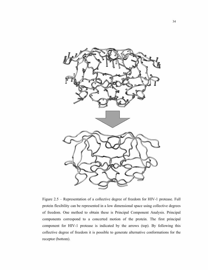
Figure 2.5 – Representation of a collective degree of freedom for HIV-1 protease. Full

protein flexibility can be represented in a low dimensional space using collective degrees

of freedom. One method to obtain these is Principal Component Analysis. Principal

components correspond to a concerted motion of the protein. The first principal

component for HIV-1 protease is indicated by the arrows (top). By following this

collective degree of freedom it is possible to generate alternative conformations for the

receptor (bottom).

35

An alternative method of calculating collective degrees of freedom for

macromolecules is the use of dimensional reduction methods. The most commonly used

dimensional reduction method for the study of protein motions is principal component

analysis (PCA). This method was first applied by Garcia (Garcia 1992) in order to

identify high-amplitude modes of fluctuations in macromolecular dynamics

simulations. It has also been used to identify and study protein conformational substates

(Romo, Clarage et al. 1995; Caves, Evanseck et al. 1998; Kitao and Go 1999), as a

possible method to extend the timescale of molecular dynamics simulations (Amadei,

Linssen et al. 1993; Amadei, Linssen et al. 1996; Abseher and Nilges 2000) and as a

method to perform conformational sampling (de Groot, Amadei et al. 1996; de Groot,

Amadei et al. 1996; Abseher and Nilges 2000). In Chapter 4, we present a protocol

(Teodoro, Phillips et al. 2003) based on PCA to derive a reduced basis representation of

protein flexibility that can be used to decrease the complexity of modeling

protein/ligand interactions. The most significant principal components have a direct

physical interpretation. They correspond to a concerted motion of the protein where all

the atoms move in specific spatial directions and with fixed ratios in overall

displacement. An example is provided in Figure 2.5,. where the directions and ratios are

indicated by the direction and size of the arrows, respectively. By considering only the

most significant principal components as the valuable degrees of freedom of the

system, it is possible to cut down an initial search space of thousands of degrees of

freedom to less than fifty. This is achievable because the fifty most significant principal

components usually account for 80-90% of the overall conformational variance of the

36

system. The PCA approach avoids some of the limitations of normal modes such as

deficient solvent modeling and existence of multiple energy minima during a large

motion. The last limitation contradicts the initial assumption of a single well energy

potential.

An alternative representation of receptor flexibility that uses a concept similar to

collective degrees of freedom, is based on the concept of molecular hinges (Sandak,

Nussinov et al. 1995; Sandak, Nussinov et al. 1998; Sandak, Wolfson et al. 1998). This

research is based on methods from the fields of computer vision and robotics. The

hinge-bending approach was originally used to model flexibility of the ligand, but the

roles of the ligand and the protein can be swapped since the mathematical problem is

symmetrical. Hinges are articulation points placed at specific locations in the protein

that allow for relative movement of domains or substructural parts. A few simultaneous

hinges can be modeled. These hinge points do not correspond to single degrees of

freedom of the original model but are instead articulations that are allowed to rotate in

three dimensions, implicitly representing rotations about consecutive or nearby bonds.

The ligand is also considered flexible and the search for a docking conformation is done

simultaneously, mimicking the induced fit process. Like pliers closing on a screw, the

receptor adapts its shape to that of the ligand. This method does not model

conformational changes for sidechains explicitly. However, it models large

conformational changes efficiently and can be easily combined with some of the

methods described above in order to model conformational changes for specific areas of

the receptor at an atomistic level. One of the main problems of the molecular hinges

37

approach is determining the location of the hinges. Recently, Jacobs et al. (Jacobs,

Rader et al. 2001) introduced a flexibility prediction algorithm based on graph theory

which can help solve this problem. The algorithm computes a constraint network for the

protein defined by the bonds (covalent and hydrogen) and salt bridges and identifies all

the rigid and flexible substructures in the protein, including overconstrained regions and

underconstrained or flexible regions.

Using collective degrees of freedom as a flexibility representation has a number

of advantages and disadvantages. One advantage is that protein flexibility is not limited

to a specific small region of the protein as was the case when using only select degrees

of freedom. Furthermore, because only a few independent degrees of freedom are used

in the optimization procedure, the computational cost is similar to using only select

degrees of freedom and is much less than the cost of techniques that consider all

degrees of freedom, such as traditional molecular dynamics or Monte Carlo. On the

other hand, the degrees of freedom that are searched during the drug design procedure

are not the native degrees of freedom of the protein, but collective modes of motion that

try to account for most of the variance observed during protein motion. This may result

in a loss of accuracy and difficulty in obtaining exact solutions. For example, there may

not exist a combination of values for the reduced basis formed by the most significant

collective degrees of freedom that results in the exact placement of all binding site

sidechains, as observed in an experimentally determined structure. However, this is

probably a minor problem since exact solutions are rarely obtained using other

methods, either. As shown in (Teodoro, Phillips et al. 2003) and Chapter 5, it is

38

possible to obtain very good approximations using only a small number of collective

degrees of freedom. Furthermore, in order to avoid high energy penalties that might

result from van der Waals clashes, it is possible to combine collective modes of motion

with either a soft receptor representation or with a post-processing minimization

procedure.

2.3. Summary

The problem of incorporating receptor flexibility in routine in silico screening

of databases of small chemical compounds for the purposes of structure based drug

design is still an unsolved problem. The main reason behind this difficulty is the large

number of degrees of freedom that have to be considered to represent receptor

flexibility. In this chapter we reviewed protein flexibility models that have been

developed to limit the number of additional search parameters. These models can be

roughly divided into five different categories. These are a) use of soft receptors which

relax energetic penalties due to steric clashes, b) selection of a few critical degrees of

freedom in the receptor binding site, c) use of multiple receptor structures either

individually or by combining them using an averaging scheme, d) use of modified

molecular simulation methods, and e) use of collective degrees of freedom as a new

basis of representation for protein flexibility. All these flexible receptor models strive to

balance an improvement in the accuracy of the binding predictions with an increase in

computational cost.

39

Chapter 3.

Tolerance Assessment of Rigid-Protein Docking Methods

to Induced Fit Effects

3.1. Introduction

A major advance in pharmaceutical drug discovery has been the ability to

computationally determine the three dimensional conformation of the complex formed

between a small ligand and a large biomacromolecule (Kuntz, Blaney et al. 1982). This

procedure, known as docking, led to a novel method for developing drugs. Instead of

physically screening millions of chemical compounds in the laboratory in search of

pharmacological activity, it was now possible to carry out the same tests in silico at a

fraction of the initial cost. Using the new method, large databases of chemically diverse

small molecules are screened to determine which are able to bind effectively to a target

receptor. The best candidates are then later optimized using both computational and

experimental methods to produce drug candidates that must undergo further laboratory

and clinical trials before final approval. During the last two decades we have seen the

emergence of different algorithms and software packages for docking. For recent

reviews on docking methods see (Muegge and Rarey 2001; Halperin, Ma et al. 2002).

However, the development of docking methods is still a work in progress and these

software packages will often fail to predict the three dimensional structures and

affinities of the bound complexes. The most common reasons for failure are

40

oversimplified energy models, poor solvent modeling and lack of representation for

receptor flexibility. In Chapter 3 we will focus on the last problem and perform a

quantitative assessment of the consequences of modeling the receptor as a rigid

structure.

Due to computational limitations, the first generation of docking programs

followed the lock-and-key model first described by Fischer (Fischer 1894). In this

model the three dimensional structure of the receptor and the ligand complement each

other in the same way that a lock complements a key. The role of the docking programs

was to find the best geometric and chemical match between two rigid structures.

Unfortunately, the lock-and-key model is a crude approximation of the binding process

which is better described by an induced-fit process (Koshland 1958) in which the three

dimensional structure of the ligand and the receptor adapt to each other during binding.

To partially address this limitation, the second generation of docking programs modeled

some of the induced-fit effect by considering a flexible ligand binding to a rigid

receptor. This is a reasonable approximation because the ligand is usually the more

flexible of the two molecules. Furthermore, ligand flexibility can be usually modeled

using only 5 to 15 degrees of freedom, whereas the full flexibility of a large

biomacromolecule can require the inclusion of more than 1000 degrees of freedom

(Teodoro, Phillips et al. 2001). Although, such a level of complexity is currently

computationally intractable a number of approximations have been proposed to

overcome this problem and are being used to develop a third generation of docking

programs which are able to model the flexibility of both the ligand and the receptor. For

41

an extensive review of current protein flexibility for structure-based drug design see

Chapter 2.

Although we are now starting to see the emergence of the third generation of

docking programs, second generation programs are still the most used in both academia

and industry settings. In practice, second generation programs are still computationally

more efficient than those that try to account for protein flexibility. Given the

widespread use and availability of second generation programs we decided to

quantitatively evaluate the extent to which the rigid-receptor/flexible-ligand docking

model can be used effectively. For this purpose we selected two commonly used

docking programs, Autodock (Morris, Goodsell et al. 1998), and DOCK (Ewing and

Kuntz 1997), and three protein models for which protein flexibility has been shown to

play a critical role during the binding process, HIV-1 protease (Wlodawer and

Vondrasek 1998), dihydrofolate reductase (DHFR) (Bystroff and Kraut 1991) and

aldose reductase (Wilson, Tarle et al. 1993). We used both docking programs to

determine if accurate docking results could be obtained for increasingly different

binding site conformations from the ones determined experimentally using X-ray

crystallography. Our work extends an earlier investigation by Murray et al (Murray,

Baxter et al. 1999) in which the authors tested whether the assumption of a rigid

enzyme compromises the accuracy of docking results. That test was carried out using

all-pairs docking for a series of three proteins. Murray et al determined that that the

assumption of a rigid active site can lead to errors in identification of the correct

42

binding mode and the assessment of binding affinity but did not quantitatively

determine to what extent current programs are able to deal with receptor model errors.

In the present work we try to address the following question: “What is the level

of similarity necessary between a receptor structural model and the actual experimental

structure to obtain useful results using second generation docking programs?”. This is

an important question because in practical docking applications the receptor model is

often an approximation of the real three dimensional conformation of the receptor when

bound with the small molecule used for the docking trial. The measure of receptor

similarity used in this work is the Root Mean Square Deviation (RMSD) for the atoms

that constitute the binding site of the different protein models. Our objective in this

work is not to evaluate the efficacy of different docking programs in dealing with the

flexible receptor problem. Our main objectives are to quantify the limitations of second

generation docking programs and to understand the range of problems that should be

addressed by third generation programs.

3.2. Materials and Methods

3.2.1. Model Systems

The coordinates for the model systems used in this study were all determined

using X-ray crystallography and obtained from the Protein Data Bank (PDB) (Berman,

Westbrook et al. 2000). The PDB codes are 1HVR (Lam, Jadhav et al. 1994) (HIV-1

protease complex with Xk263 of Dupont Merck), 4DFR (Bolin, Filman et al. 1982)

43

(dihydrofolate reductase complex with methotrexate), and 1AH3 (Urzhumtsev, Tete-

Favier et al. 1997) (aldose reductase complex with tolrestat).

3.2.2. Conformational Sampling

Conformational sampling of the receptor structures was obtained using a simple

molecular dynamics based method. Molecular dynamics has been often used as a

method to model the conformational flexibility of the receptor during binding processes

(Di Nola, Roccatano et al. 1994; Luty, Wasserman et al. 1995; Wasserman and Hodge

1996; Mangoni, Roccatano et al. 1999; Pak and Wang 2000). In this study we used high

temperature molecular dynamics (Bruccoleri and Karplus 1990). The advantages of this

technique are its simplicity and high computational efficiency. In contrast to earlier

studies, the objective of the molecular dynamics step is not to exhaustively explore the

conformational space of the protein as it binds to a ligand. We used molecular

dynamics in order to obtain a small set of alternative protein conformations that

represented different levels of similarity from the original X-ray structure. Simulations

were carried out using the NAMD2 program (Kalé, Skeel et al. 1999) and the

CHARMM forcefield (MacKerell, Bashford et al. 1998). The receptor structures were

prepared by removing ligands (Xk263, methotrexate, and tolrestat) and water

molecules. After an initial minimization using a conjugate gradient method, the

receptor structures were simulated at a temperature of 800K for 50ps using a 1fs

integration timestep. Non-bonded interactions were truncated at distances larger than

12Å. To avoid a discontinuity in the non-bonded potential at the cutoff distance a

switching function was used starting at 9Å. Conformational snapshots were written to

44

disk every 100fs. The high temperature simulation was run 20 times for each system

using different random seeds for initial velocity assignment to improve the

conformational sampling. The conformational snapshots for the 20 simulations were

combined into a single large pool and were superimposed on the original crystal

structure using a least squares procedure (Kabsch 1976).

Although the whole protein was simulated using molecular dynamics, we

restricted the analysis of the results to the residues that constitute the binding site region

of the three proteins. The reason is that conformational changes at the level of the

binding site play the most significant role in determining the results of docking. The

residues were chosen by visual inspection of the experimental bound conformations.

The residues considered for each protein are shown in Table 3.1.

Protein Residues included in RMSD calculation

HIV-1 Protease

(PDB code: 1HVR)

8, 23, 25, 27-32 , 47-50, 80-84

(monomers A and B)

Dihydrofolate Reductase

(PDB code: 4DFR)

5, 7, 27, 28, 31, 32, 46, 49, 50, 52, 54, 57, 94

Aldose Reductase

(PDB code: 1AH3)

20, 47, 48, 79, 110, 111, 113, 115, 122, 130, 219, 298, 300,

302, 303

Table 3.1 – Residue numbers included in binding site RMSD calculation.

From the pool obtained using molecular dynamics we formed 10 groups of 10

structures, such that structures in the same group had similar RMSD to the X-ray

structure. The RMSD groups considered were from 0.1Å to 1.9Å in steps of 0.2Å.

45

Figure 3.1 illustrates the conformational variation present in the different RMSD groups

for HIV-1 protease. The selected RMSD range of conformational variation was in

accordance to what was observed in many cases for proteins deposited in the PDB

(Berman, Westbrook et al. 2000). It is common for proteins to differ by as much as 2Å

RMSD between their bound and unbound forms or even when bound to different

ligands. In some cases, such as the protein calmodulin, conformational changes upon

binding are much larger than 2Å. We decided not to include such large conformational

changes in our study since they are usually beyond what can be tackled using second

generation docking program.

46

Figure 3.1 - Conformational sampling of binding site conformations. a) The

experimentally determined structure of the model proteins (HIV-1 protease shown) was

used as a starting point for a high temperature molecular dynamics simulation. The entire

protein backbone is shown in blue and the residues defining the shape of the binding site

are highlighted in yellow. In b) we show a magnified view of the binding site displaying

only the residues used for the RMSD calculations. c) The multiple conformational

snapshots resulting from the sampling simulations were sorted and grouped according to

the RMSD to the original experimental structure. In c) we show the superposition of 10

representative structures for eight different similarity groups. Structures from these

groups were subsequently used for docking as representatives of different levels of

conformational flexibility.

47

3.2.3. Autodock

Ligand and protein input files were prepared as suggested in the Autodock

manual. Ligand atom coordinates were obtained from the original PDB files. Hydrogen

atom coordinates and Gasteiger-Marsili (Gasteiger and Marsili 1980) charges for all

ligand atoms were calculated using SYBYL V6.8 (Tripos Associates, St Louis, MO). In

order to test the effects of ligand flexibility on the docking results ligand input files

were prepared for different degrees of conformational flexibility. Xk263 was modeled

using 0, 4, and 10 degrees of freedom. Methotrexate was modeled using 0, 4, and 12

degrees of freedom. Tolrestat was modeled using 0 and 6 degrees of freedom. The

bonds which were defined to be rotatable on the different levels of flexibility are

illustrated in Figure 3.2. In the case where 0 degrees of freedom were used to model the

flexibility of the ligand (i.e., rigid ligand), the ligand conformation was taken directly

from the original X-ray structure.

Protein atom coordinates were obtained from the snapshots of the molecular

dynamics simulations. All hydrogen atoms were removed from the protein. SYBYL

was then used to re-add polar hydrogens and to assign Kollman united-atom partial

charges to the protein. Atomic solvation parameters and fragmental volumes were

assigned to the protein atoms using ADDSOL. The resulting structures were used to

calculate interaction energy grid maps using AutoGrid. Grids were calculated for an

axis aligned cube of side 22.5Å centered on the geometric center of the ligand in the

original crystal structure. Grid spacing was 0.375Å. Default AutoGrid values were used

for the remaining parameters. The resulting grids and the ligand files were used as input

48

for Autodock V3.0.5. Docking was carried out using the Lamarckian Genetic

Algorithm (LGA) search method. The following values were used for the genetic

algorithm parameters: the number of individuals in population was 50; the maximum

number of energy evaluations was 1500000; the maximum number of generations was

27000; the elitism was 1; the rate of gene mutation was 0.02; the rate of crossover was

0.80; the number of generations for picking worst individual was 10; the mean of

Cauchy distribution for gene mutation was 0; the variance of Cauchy distribution for

gene mutation was 1. Local search was carried out using the pseudo Solis and Wets

local optimizer using the following parameter values: the maximum number of

iterations per local search was 300; the probability of performing local search on an

individual in the population was 0.06; the maximum number of consecutive successes

or failures before doubling or halving the local search step size, , was 4, in both cases;

and the lower bound on , the termination criterion for the local search, was 0.01. The

search for a docked conformation was repeated 10 times for each initial protein

conformation. The results reported refer to the conformation with the lowest interaction

energy score as reported by Autodock. RMSD values reported are from the ligand

coordinates in the lowest energy conformation using as reference the crystallographic

coordinates of the ligand.

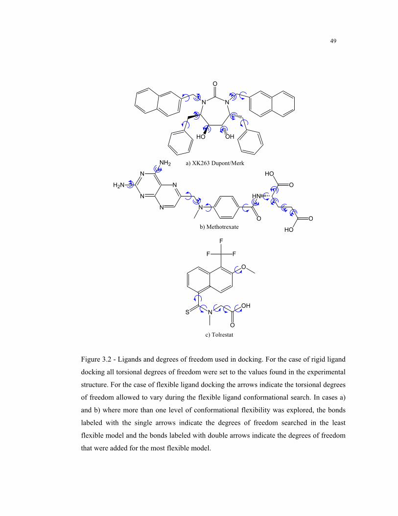
49

N N

O

HO OH

a) XK263 Dupont/Merk

b) Methotrexate

HN

O

HO

O

HO

O

N

N

N

N

N

NH2

H2N

N

O

OHS

FF

F

O

c) Tolrestat

Figure 3.2 - Ligands and degrees of freedom used in docking. For the case of rigid ligand

docking all torsional degrees of freedom were set to the values found in the experimental

structure. For the case of flexible ligand docking the arrows indicate the torsional degrees

of freedom allowed to vary during the flexible ligand conformational search. In cases a)

and b) where more than one level of conformational flexibility was explored, the bonds

labeled with the single arrows indicate the degrees of freedom searched in the least

flexible model and the bonds labeled with double arrows indicate the degrees of freedom

that were added for the most flexible model.

50

3.2.4. Dock

Ligand and protein input files were prepared in the same manner was described

above for Autodock with the exception that all hydrogens were added to the protein

representation as required by DOCK. Spheres characterizing the binding site were

generated using the program SPHGEN as described in (Kuntz, Blaney et al. 1982) and

edited in order to remove spheres far from the binding site. Interaction energy scoring

grids were generated using the program GRID. The grid size and positions were

calculated such that they would enclose the cluster of spheres representing the binding

site. An extra margin of 5Å in all directions was added to the grid sizes. The size of the

grids computed was variable but was approximately the size of the grids computed for

scoring in Autodock. Grid spacing was 0.300Å. Default GRID values were used for the

remaining parameters. The resulting grids and the ligand files were used as input for

DOCK V4.0. The following values were used for the DOCK parameters: the maximum

number of orientations tried was 10,000 using automated matching and a matching

tolerance of 0.25Å. Default values were used for the remaining docking parameters.

Torsion minimization was used in the case of flexible ligand models. One cycle of

minimization was also used to adjust the orientation and conformation of the ligand and

improve its interaction energy score. The minimization used a maximum of 100 steps,

an initial translation step of 0.5Å, an initial rotation step of 0.1 degrees, and an initial

torsion step of 10 degrees. The reported results refer to the conformation with the

lowest interaction energy score as reported by DOCK.

51

3.3. Results and Discussion

The original experimentally determined conformation and the derived structures

obtained using high temperature molecular dynamics were used as input for the docking

programs Autodock and DOCK. This corresponded to 101 alternative receptor

conformations considered for each of the proteins. Alternative levels of ligand

flexibility were also tested. The results for the docking experiments are shown in

Figures 3.3 through 3.5. Each of the plots contains the following information. The axis

of abscissas represents the different conformational variation groups. The 100

computationally generated protein conformations are grouped in 10 sets according to

the RMSD values of non-hydrogen atoms of residues that constitute the binding site

using as a reference the crystal structure. On the right axis of ordinates and shown in

open circles connected by lines is the average interaction energy score for each

conformational group. On the left axis of ordinates and shown using filled rhombs are

the ligand RMSD values for the lowest energy docked solution using as a reference the

position of the ligand in the crystal structure. The circle and the cross over the left axis

of ordinates indicate the interaction energy score and ligand RMSD using the

experimental receptor conformation, respectively. Theoretically, if docking programs

were able to reproduce exactly experimental ligand bound conformations the ligand

RMSD value should be 0.0Å. Due to errors and approximations present in interaction

energy scoring functions the conformation corresponding to the global minimum of the

scoring function never matches exactly the conformation determined experimentally.

Nevertheless, this value is usually very close to the experimental value. The ligand

52

RMSD values we obtained for docking with the crystal structure of HIV-1 protease,

DHFR, and aldose reductase using Autodock are 0.36Å, 0.60Å, and 0.69Å respectively.

The same values using the DOCK program are 0.25Å, 0.69Å, and 0.53Å. These

numbers provide a baseline for what are the best results that can be expected using the

above model systems. In this study we considered that any result better than 1.5Å

corresponds to the correct docked orientation. This value is similar to values chosen for

other docking studies(Rarey, Kramer et al. 1996; Jones, Willett et al. 1997; Paul and

Rognan 2002). Furthermore, in order to avoid any bias we did not select the solution

with lowest ligand RMSD as the best solution from each docking run. The best solution

selected was the one with the lowest interaction energy value.

Figure 3.3 shows the results obtained for both rigid and flexible ligand models

using the Autodock program. The rationale for testing the effects of ligand flexibility in

conjunction with receptor flexibility was to assess to what extent a flexible ligand

model would compensate for changes in the receptor. For example, conformational

changes in the receptor could be such that the original three dimensional shape of the

ligand could not fit into the binding site cavity without leading to steric clashes

resulting in a high energetic penalty. However, a flexible ligand might still lead to a

good three dimensional shape complementarity by changing its internal degrees of

freedom by a small amount in order to adapt to the new receptor shape. We also used

the rigid ligand model to compare whether it would be more adversely affected by

changes in the receptor. Furthermore, the use of multiple low energy ligand conformers

to represent a ligand in a rigid-protein/rigid-ligand virtual screening effort is still a

53

common practice. Such approach reduces the dimensionality of the conformational

space that needs to be explored in the search for the minimum energy docked

conformation. In practice we observed only small differences in the results between the

rigid and moderately flexible (4 to 6 degrees of freedom) ligand models. This is due

mainly to the fact that the conformation of the ligand used for the rigid docking was

taken directly from the crystal structure. As such, the values for its torsional degrees of

freedom are already at its optimum values which facilitated the docking search. When a

flexible ligand was used the conformational search ended up with a very similar

solution to the rigid ligand conformation. This type of result was independent of the

docking program used as can be seen from Figure 3.5. Another observation common to

all protein systems is that correct docked solutions show an increase in average ligand

RMSD for more flexible ligand models. This is not an indication that the docking

solution is worse. It is caused by small differences from the crystal structure in the

values obtained for the internal degrees of freedom which lead to an increase in ligand

RMSD. The increase in ligand RMSD is particularly noticeable for DHFR. For this

protein the average ligand RMSD for the 0.1Å receptor RMSD group are 0.59Å, 0.70Å,

and 1.23Å for the 0, 4, and 12 degrees of freedom models, respectively. However a

visual inspection of the results clearly indicates that in all solutions the generally

correct docked conformation was obtained.

54

HIV-1 Protease (0 dof)

0

1

2

3

4

5

6

7

8

9

0.0 0.2 0.4 0.6 0.8 1.0 1.2 1.4 1.6 1.8 2.0

Receptor RMSD (Å)

Lig

and

RM

SD

(Å)

-20

-18

-16

-14

-12

-10

-8

Energ

yS

core

(kcal/m

ol)

HIV-1 Protease (4 dof)

0

1

2

3

4

5

6

7

8

9

0.0 0.2 0.4 0.6 0.8 1.0 1.2 1.4 1.6 1.8 2.0

Receptor RMSD (Å)

Lig

and

RM

SD

(Å)

-20

-18

-16

-14

-12

-10

-8

Energ

yS

core

(kcal/m

ol)

Figure 3.3-a) – Autodock docking results for HIV-1 protease using a rigid (left column) or a flexible ligand (right column). The

axis of abscissas represents the different conformational variation groups for the protein. Each conformational group contains 10

representative structures. The RMSD values are for the non-hydrogen atom coordinates of the residues that constitute the

binding site using as a reference the crystal structure. On the right axis of ordinates and shown in open circles in the plot is the

average interaction energy score for each conformational group. On the left axis of ordinates and shown using filled rhombs are

the ligand RMSD values for the lowest energy docked solution using as a reference the position of the ligand in the crystal

structure. The cross over the left axis of ordinates indicates the ligand RMSD docking solution using the original receptor

structure.

55

DHFR (0 dof)

0

1

2

3

4

5

6

0.0 0.2 0.4 0.6 0.8 1.0 1.2 1.4 1.6 1.8 2.0

Receptor RMSD (Å)

Lig

and

RM

SD

(Å)

-14

-13

-12

-11

-10

-9

-8

-7

Energ

yS

core

(kcal/m

ol)

DHFR (4 dof)

0

1

2

3

4

5

6

0.0 0.2 0.4 0.6 0.8 1.0 1.2 1.4 1.6 1.8 2.0

Receptor RMSD (Å)

Lig

and

RM

SD

(Å)

-14

-13

-12

-11

-10

-9

-8

-7

Energ

yS

core

(kcal/m

ol)

Figure 3.3–b) - Autodock docking results for DHFR using a rigid (left column) or a flexible ligand (right column). The data

representation is the same as for Figure 3.3-a).

56

Aldose Reductase (0 dof)

0

1

2

3

4

5

6

7

8

9

10

0.0 0.2 0.4 0.6 0.8 1.0 1.2 1.4 1.6 1.8 2.0Receptor RMSD (Å)

Liga

ndR

MS

D(Å

)

-11

-10

-9

-8

-7

-6

-5

Energy

Score

(kcal/mol)

Aldose Reductase (6 dof)

0

1

2

3

4

5

6

7

8

9

10

0.0 0.2 0.4 0.6 0.8 1.0 1.2 1.4 1.6 1.8 2.0Receptor RMSD (Å)

Liga

ndR

MS

D(Å

)-11

-10

-9

-8

-7

-6

-5

Ene

rgy

Score

(kcal/mol)

Figure 3.3-c) - Autodock docking results for aldose reductase using a rigid (left column) or a flexible ligand (right column). The

data representation is the same as for Figure 3.3-a).

57

In almost all cases where the rigid ligand model could not be fitted in the

binding site cavity the same occurred for the flexible case. This occurred because the

change in the receptor shape was such that it drastically affected the three dimensional

properties of the binding site. An example of such change is a reorientation of a

sidechain in the center of the binding site of aldose reductase such that the binding

cavity was approximately divided into two smaller cavities. In these types of situations,

ligand flexibility is not sufficient to compensate for the receptor changes therefore

negating the advantages of this model. In addition, we also observed that the increase in

dimensionality of the search space due to the extra degrees of freedom in the ligand

sometimes resulted in failure to find the correct ligand conformation even when we

knew it existed because it was found using the rigid search. This type of behavior is

evident when we compare the results for the docking of HIV-1 protease and DHFR

using the moderate (4 torsional degrees of freedom) shown in Figures 3.3-a) and 3.3-b)

and very flexible ligand models (10 and 12 torsional degrees of freedom, respectively)

shown in Figure 3.4. In the case of HIV-1 protease the total number of docked solutions

with ligand RMSD below 1.5Å falls from 73 to 69. This effect is even more noticeable

for DHFR in which the increase in the search space is larger. In this case the number of

correct solutions falls from 43 to 35. The main conclusion from these observations

should not be that using flexible ligand models for docking is a wasted effort. In the

specific case of the present study we are trying to evaluate only the effects of receptor

flexibility on docking results. As such we are starting our ligand conformational search

from the known experimental conformation and, in the case of the flexible model,

58

letting the ligand adapt to changes in the shape of the receptor. The main observation

from the ligand flexibility results is that, for that case of the receptor/ligand pairs used

in this study, ligand flexibility did not play a major role in the docking results and the

advantages obtained from the flexible model are lost by the increase in the search space

given equal computing time.

The results obtained for the average lowest energy score for each

conformational set show the same general behavior for all protein models, docking

programs and ligand flexibility levels. For very small receptor RMSD, the energy score

is usually very similar to the score obtained using the original crystal structure (results

not shown). As the receptor RMSD increases we observe an increase in energy. The

increase in energy is always initiated even at receptor RMSD levels for which the

docking results as determined by the ligand RMSD score are still very good. This

behavior reflects the fact that although the ligand is still located in the correct area of

the binding site, the interactions it is forming with the protein are not as strong as in the

crystal structure. For very large receptor deviations the average interaction energy

reaches a plateau similar to the ligand RMSD values. This reflects final docked

orientations for the ligand which bind weakly and are very different from the original.

59

HIV-1 Protease (10 dof)

0

1

2

3

4

5

6

7

0.0 0.2 0.4 0.6 0.8 1.0 1.2 1.4 1.6 1.8 2.0

Receptor RMSD (Å)

Lig

and

RM

SD

(Å)

-22

-21

-20

-19

-18

-17

-16

-15

-14

Energ

yS

core

(kcal/m

ol)

DHFR (12 dof)

0

1

2

3

4

5

6

0.0 0.2 0.4 0.6 0.8 1.0 1.2 1.4 1.6 1.8 2.0

Receptor RMSD (Å)

Lig

and

RM

SD

(Å)

-11

-10

-9

-8

-7

Energ

yS

core

(kcal/m

ol)

Figure 3.4 - Autodock docking results for HIV-1 protease (left) and DHFR (right) using a very flexible ligand model. The data

representation is the same as for Figure 3.3-a).

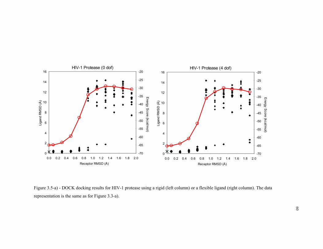
60

HIV-1 Protease (0 dof)

0

2

4

6

8

10

12

14

16

0.0 0.2 0.4 0.6 0.8 1.0 1.2 1.4 1.6 1.8 2.0

Receptor RMSD (Å)

Lig

and

RM

SD

(Å)

-70

-65

-60

-55

-50

-45

-40

-35

-30

-25

-20

Energ

yS

core

(kcal/m

ol)

HIV-1 Protease (4 dof)

0

2

4

6

8

10

12

14

16

0.0 0.2 0.4 0.6 0.8 1.0 1.2 1.4 1.6 1.8 2.0

Receptor RMSD (Å)

Lig

and

RM

SD

(Å)

-70

-65

-60

-55

-50

-45

-40

-35

-30

-25

-20

Energ

yS

core

(kcal/m

ol)

Figure 3.5-a) - DOCK docking results for HIV-1 protease using a rigid (left column) or a flexible ligand (right column). The data

representation is the same as for Figure 3.3-a).

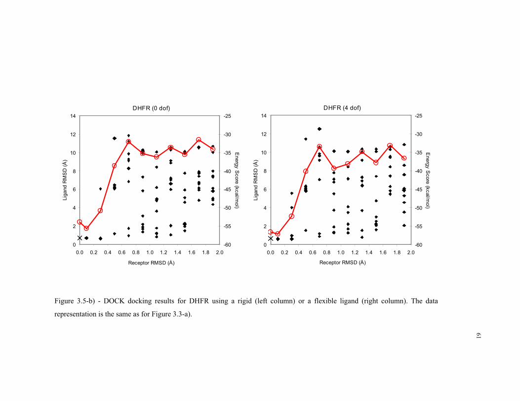
61

DHFR (0 dof)

0

2

4

6

8

10

12

14

0.0 0.2 0.4 0.6 0.8 1.0 1.2 1.4 1.6 1.8 2.0

Receptor RMSD (Å)

Lig

and

RM

SD

(Å)

-60

-55

-50

-45

-40

-35

-30

-25

Energ

yS

core

(kcal/m

ol)

DHFR (4 dof)

0

2

4

6

8

10

12

14

0.0 0.2 0.4 0.6 0.8 1.0 1.2 1.4 1.6 1.8 2.0

Receptor RMSD (Å)

Lig

and

RM

SD

(Å)

-60

-55

-50

-45

-40

-35

-30

-25

Energ

yS

core

(kcal/m

ol)

Figure 3.5-b) - DOCK docking results for DHFR using a rigid (left column) or a flexible ligand (right column). The data

representation is the same as for Figure 3.3-a).

62

Aldose Reductase (0 dof)

0

2

4

6

8

10

12

14

0.0 0.2 0.4 0.6 0.8 1.0 1.2 1.4 1.6 1.8 2.0Receptor RMSD (Å)

Lig

and

RM

SD

(Å)

-32

-30

-28

-26

-24

-22

Energy

Score

(kcal/mol)

Aldose Reductase (6 dof)

0

2

4

6

8

10

12

14

0.0 0.2 0.4 0.6 0.8 1.0 1.2 1.4 1.6 1.8 2.0Receptor RMSD (Å)

Liga

ndR

MS

D(Å

)-32

-30

-28

-26

-24

-22

Energy

Score

(kcal/mol)

Figure 3.5-c) - DOCK docking results for aldose reductase using a rigid (left column) or a flexible ligand (right column). The

data representation is the same as for Figure 3.3-a).

63

One of the main motivations for this study was to determine what level of

receptor similarity is necessary between a structural model and the actual experimental

structure in order to obtain a correct docking result. This type of information is valuable

because it is common practice in virtual screening to use as a target, a receptor

structural model that differs from what would be the actual experimental structure

bound to the ligand being tested. This receptor model can originate from an

experimental structure of a complex with another ligand or from a homology model.

The results we obtained are clearly protein dependent. Using the Autodock program we

can observe from Figure 3.3 that, whereas for HIV-1 protease all structures in the

conformational sets with receptor RMSD lower than 1.0Å are able to correctly dock

rigid models of XK263, for aldose reductase there are 14 structural models that fail to

find the correct docked conformation for a rigid model of tolrestat. Using a flexible

model of tolrestat there are 20 failed dockings. From the plots in Figure 3.3 we can

derive that HIV-1 protease docking seems to be very tolerant of variations in the

conformation of the receptor. In fact almost all of the docking experiments with

receptor models for which the RMSD to the crystal structure is less than 1.2Å result in

correct docking results. In the case of aldose reductase this number drops to 0.6Å.

DHFR results are similar to HIV-1 protease, but there is a larger difference depending

on the level of flexibility of the ligand model. Whereas most results below 1.4Å

receptor RMSD find ligand conformations similar to the one observed in the

experimental structure in the rigid ligand case, this threshold drops to approximately

0.8Å in the flexible case. The results using DOCK (Figure 3.4) for HIV-1 protease and

64

for aldose reductase show a similar behavior although with different threshold values.

HIV-1 protease and aldose reductase show correct results up to 0.8Å and 0.4Å receptor

RMSD respectively. On the other hand the results seem to be minimally affected by the

presence of ligand flexibility. These types of differences between docking programs are

not significant and are fairly dependent on the input parameter values chosen to run the

program. Due to the fact that there we were not trying to compare docking programs we

decided to use the recommended parameters by the authors of these programs. The

largest difference in results between Autodock and DOCK was for DHFR. In this case

there are several positive results for receptor conformations as different as 1.5Å but

there are also several docking failures for values as low as 0.3Å. The worse results are

due to some difficulty in the DOCK scoring function in identifying the correct docked

conformation as the one with lowest interaction energy. For the case of DHFR it was

common to find the correct docked conformation as a lower ranking conformation in

terms of energy score. Autodock and DOCK use very different scoring functions and as

such it is not surprising to see cases in which one of the scoring functions works better

than other for a particular protein system. Energy scoring functions are probably the

most critical part of a docking system and problems like these are common. For recent

reviews on this topic see (Tame 1999; Gohlke and Klebe 2001; Muegge and Rarey

2001; Halperin, Ma et al. 2002).

The results obtained in the present study clearly indicate that the effectiveness

of second generation docking programs in dealing with receptor flexibility is protein

dependent. This provides further insight into why structure-based drug design efforts

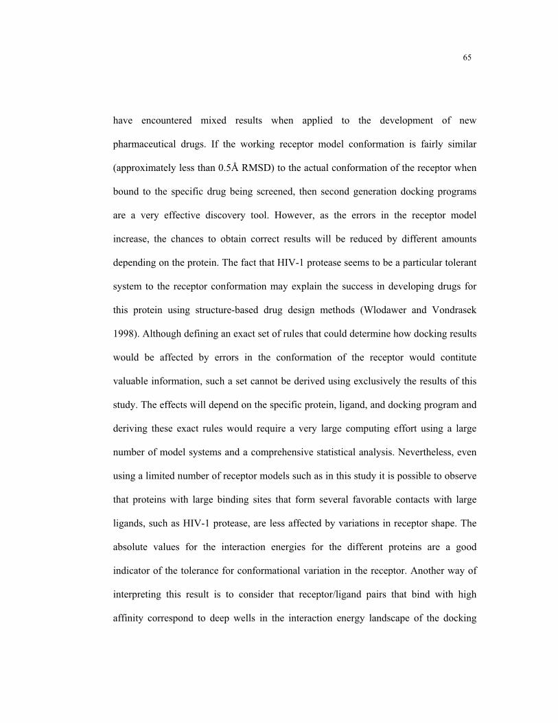
65

have encountered mixed results when applied to the development of new

pharmaceutical drugs. If the working receptor model conformation is fairly similar

(approximately less than 0.5Å RMSD) to the actual conformation of the receptor when

bound to the specific drug being screened, then second generation docking programs

are a very effective discovery tool. However, as the errors in the receptor model

increase, the chances to obtain correct results will be reduced by different amounts

depending on the protein. The fact that HIV-1 protease seems to be a particular tolerant

system to the receptor conformation may explain the success in developing drugs for

this protein using structure-based drug design methods (Wlodawer and Vondrasek

1998). Although defining an exact set of rules that could determine how docking results

would be affected by errors in the conformation of the receptor would contitute

valuable information, such a set cannot be derived using exclusively the results of this

study. The effects will depend on the specific protein, ligand, and docking program and

deriving these exact rules would require a very large computing effort using a large

number of model systems and a comprehensive statistical analysis. Nevertheless, even

using a limited number of receptor models such as in this study it is possible to observe

that proteins with large binding sites that form several favorable contacts with large

ligands, such as HIV-1 protease, are less affected by variations in receptor shape. The

absolute values for the interaction energies for the different proteins are a good

indicator of the tolerance for conformational variation in the receptor. Another way of

interpreting this result is to consider that receptor/ligand pairs that bind with high

affinity correspond to deep wells in the interaction energy landscape of the docking

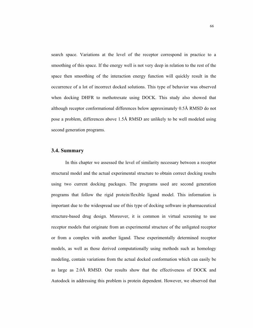
66

search space. Variations at the level of the receptor correspond in practice to a

smoothing of this space. If the energy well is not very deep in relation to the rest of the

space then smoothing of the interaction energy function will quickly result in the

occurrence of a lot of incorrect docked solutions. This type of behavior was observed

when docking DHFR to methotrexate using DOCK. This study also showed that

although receptor conformational differences below approximately 0.5Å RMSD do not

pose a problem, differences above 1.5Å RMSD are unlikely to be well modeled using

second generation programs.

3.4. Summary

In this chapter we assessed the level of similarity necessary between a receptor

structural model and the actual experimental structure to obtain correct docking results

using two current docking packages. The programs used are second generation

programs that follow the rigid protein/flexible ligand model. This information is

important due to the widespread use of this type of docking software in pharmaceutical

structure-based drug design. Moreover, it is common in virtual screening to use

receptor models that originate from an experimental structure of the unligated receptor

or from a complex with another ligand. These experimentally determined receptor

models, as well as those derived computationally using methods such as homology

modeling, contain variations from the actual docked conformation which can easily be

as large as 2.0Å RMSD. Our results show that the effectiveness of DOCK and

Autodock in addressing this problem is protein dependent. However, we observed that

67

independently of the protein system, receptor errors below approximately 0.5Å RMSD

do not pose a problem, whereas errors above 1.5Å RMSD will likely result in docking

failures.

68

Chapter 4.

Calculation of Protein Collective Modes of Motion Using

Dimensional Reduction Methods

4.1. Introduction

The functions of proteins can be as varied as enzymatic catalysis, mechanical

support, immune protection and generation and transmission of nerve impulses among

many others. Today there is a large body of knowledge available on protein structure

and function as a result of several decades of intense research by scientists worldwide.

This information is expected to grow at an even faster pace in the coming years due to

new efforts in large-scale proteomics and structural genomics projects. In order to make

the best use of the exponential increase in the amount of data available, it is imperative

that we develop automated methods for extracting relevant information from large

amounts of protein structural data. The focus of this chapter is on how to obtain a

reduced representation of protein flexibility from raw protein structural data.

Current structural biology experimental methods are restricted in the amount of

information they can provide regarding protein motions because they were designed

mainly to determine the three-dimensional static representation of a molecule. The two

most common methods in use today are protein X-ray crystallography (Rhodes 1993)

and nuclear magnetic resonance (NMR) (Wüthrich 1986). The output of these

techniques is a set of {x, y, z} coordinate values for each atom in a protein. Neither of

69

these methods is able to provide us with a full description, at atomic resolution, of the

structural changes that proteins undergo in a timescale relevant to their function. Such

information would be ideal to understand and model proteins. The alternative to

experimental methods is to use computational methods based on classical (Brooks,

Montgomery et al. 1988) or quantum mechanics (Gogonea, Suarez et al. 2001) to

approximate protein flexibility. However these computations are prohibitively

expensive and are not suitable for potential target applications such as the ones

described in the previous paragraph. One of the reasons why the above computational

methods are expensive is that they try to simulate all possible motions of the protein

based on physical laws. For the case of molecular dynamics, the timestep for the

numerical integration of such simulations needs to be small (in the order of

femtoseconds), while relevant motions occur in a much longer timescale (microseconds

to milliseconds). It is unrealistic to expect that one could routinely use molecular

dynamics or quantum mechanics methods to simulate large conformational

rearrangements of molecules. A medium sized protein can have as many as several

thousand atoms and each atom can move along three degrees of freedom. Even when

considering more restricted versions of protein flexibility that take into account only

internal torsional degrees of freedom, or restrict the degrees of freedom to take only a

set of discrete values, exploring the conformational space of these proteins is still a

formidable combinatorial search problem (Finn and Kavraki 1999).

The method presented in this chapter addresses the high-dimensionality problem

by transforming the basis of representation of molecular motion. Whereas in the

70

standard representation all degrees of freedom (the {x, y, z} values for each atom) of

the molecule were of equal importance, in the new representation the new degrees of

freedom will be linear combinations of the original variables in such way that some

degrees of freedom are significantly more representative of protein flexibility than

others. As a result, we can approximate the total molecular flexibility by truncating the

new basis of representation and considering only the most significant degrees of

freedom. The remaining degrees of freedom can be disregarded resulting in only a

small inaccuracy in the molecular representation. Transformed degrees of freedom will

no longer be single atom movements along the Cartesian axes but collective motions

affecting the entire configuration of the protein. The main tradeoff of this method is that

there is some loss of information due to truncation (of the new basis) but this factor is

outweighed by the ability to effectively model protein flexibility in a subspace of

largely reduced dimensionality. We also show that results are acceptable, consistent

with experimental laboratory results, and help shed light on the mechanisms of

biomolecular processes.

4.2. Background

4.2.1. Dimensional Reduction Methods

Dimensionality reduction techniques aim to determine the underlying true

dimensionality of a discrete sampling X of an n-dimensional space. That is, if X is

embedded in a subspace of dimensionality m, where m<n, then we can find a mapping

F:X Y such that Y B and B is an m-dimensional manifold. Dimensionality reduction

71

methods can be divided into two types: linear and non-linear. The two most commonly

used linear methods to find such mappings are Multi-Dimensional Scaling (MDS) and

Principal Component Analysis (PCA).

MDS encompasses a variety of multivariate data analysis techniques that were

originally developed in mathematical psychology (Shepard 1962; Kruskal 1964) to

search for a low-dimensional representation of high-dimensional data. The search is

carried out such that the distances between the objects in the lower dimensional space

match as well as possible, under some similarity measure between points in the original

high-dimensional space.

PCA is a widely used technique for dimensionality reduction. This method,

which was first proposed by Pearson (Pearson 1901) and further developed by

Hotelling (Hotelling 1933), involves a mathematical procedure that transforms the

original high-dimensional set of (possibly) correlated variables into a reduced set of

uncorrelated variables called principal components. These are linear combinations of

the original values in which the first principal component accounts for most of the

variance in the original data, and each subsequent component accounts for as much of

the remaining variance as possible. Note that if the similarity measure of MDS

corresponds to the Euclidean distances then the results of MDS are equivalent to PCA.

The MDS and PCA dimensionality reduction methods are fast to compute, simple to

implement, and since their optimizations do not involve local minima, they are

guaranteed to discover the dimensionality of a discrete sample of data on a linear

subspace of the original space.

72

One of the limitations of methods such as MDS and PCA is that their

effectiveness is restricted by the fact that they are globally linear methods. As a result,

if the original data is inherently non-linear these methods will represent the true

reduced manifold in a subspace of higher dimension than necessary in order to cover

non-linearity. This problem is likely to occur with protein motion data (Garcia 1992).

To overcome this limitation several methods for non-linear dimensionality reduction

have been proposed in recent years. Among these are principal curves (Hastie and

Stuetzle 1989; Tibshirani 1992), multi-layer auto-associative neural networks (Kramer

1991), local PCA (Kambhatla and Leen 1997; Meinicke and Ritter 1999), mixtures of

principal components formulated within a maximum-likelihood framework (Tipping

and Bishop 1999), generative topographic mapping (Bishop, Svensen et al. 1998), and

genetic algorithms (Raymer, Punch et al. 2000). More recently Tenenbaum et al

proposed the isomap method (Tenenbaum, de Silva et al. 2000) and Roweis and Saul

proposed the locally linear embedding method (Roweis and Saul 2000). The main

advantage of the last two methods is that the optimization procedure used to find the

low-dimensional embedding of the data does not involve local minima. In general the

main disadvantages of non-linear versus linear dimensionality reduction methods are

increased computational cost, difficulty of implementation, and problematic

convergence. The development of new methods for dimensionality reduction is an

active research area.

73

4.2.2. Collective Coordinate Representation of Protein Dynamics

The application of dimensionality reduction methods, namely PCA, to macromolecular

structural data was first described by Garcia in order to identify high-amplitude modes

of fluctuations in macromolecular dynamics simulations (Garcia 1992). It as also been

used to identify and study protein conformational substates (Romo, Clarage et al. 1995;

Caves, Evanseck et al. 1998; Kitao and Go 1999), to identify domain motions

(Chillemi, Falconi et al. 1997), as a possible method to extend the timescale of

molecular dynamics simulations (Amadei, Linssen et al. 1993; Amadei, Linssen et al.

1996), and as a method to perform conformational sampling (de Groot, Amadei et al.

1996; de Groot, Amadei et al. 1996). The validity of the method has also been

established by comparison with laboratory experimentally derived data (van Aalten,

Conn et al. 1997; de Groot, Hayward et al. 1998). As a substitute to the use of direct

coordinate information for the computation of the principal components it is also

possible to use this method with atomic distances information (Abseher and Nilges

1998). An alternative approach to determine collective modes for proteins uses normal

mode analysis (Levy and Karplus 1979; Go, Noguti et al. 1983; Levitt, Sander et al.

1985; Case 1994) and can also serve as a basis for modeling the flexibility of large

molecules (Kolossvary and Guida 1999; Zacharias and Sklenar 1999; Keseru and

Kolossvary 2001; Kolossvary and Keseru 2001). Normal mode analysis is a direct way

to analyze vibrational motions. To determine the vibrational motions of a molecular

system, the eigenvalues and the eigenvectors of a mass weighted matrix of the second

derivatives of the potential function are computed. The eigenvectors correspond to

74

collective motions of the molecule and the eigenvalues are proportional to the squares

of the vibrational frequencies. Direct comparisons of PCA and normal modes based

methods have been published (Hayward, Kitao et al. 1997; van Aalten, de Groot et al.

1997). The PCA approach described in this chapter avoids some of the limitations of

normal modes such as lack of solvent modeling, assumption that the potential energy

varies quadratically, and existence of multiple energy minima during large

conformational transitions. In contrast to previously published work, we focus on the

interpretation of the principal components as biologically relevant motions and on how

combinations of a reduced number of these motions can approximate alternative

conformations of the protein. More recently other collective coordinate models such as

the Gaussian network (Bahar, Erman et al. 1999), the “Jumping-Among- Minima”

(Kitao, Hayward et al. 1998), and space warping (Jaqaman and Ortoleva 2002) have

been applied to the study of proteins and DNA. For general reviews on the use of

collective coordinate representations to model biomacromolecules see (Hayward and

Go 1995; Kitao and Go 1999; Lafontaine and Lavery 1999).

4.3. Methods

4.3.1. Molecular Dynamics Data

Molecular dynamics simulations were carried out using similar protocols for all

model systems. The protocol for HIV-1 protease will be described in detail and specific

differences will be shown in parentheses. The HIV-1 protease simulation was computed

using the program NAMD2 (Kalé, Skeel et al. 1999) and the Charmm22 parameter set

75

(MacKerell, Bashford et al. 1998). The starting coordinates for HIV-1 protease used in

the simulations originated from the crystal structure published by Miller and

collaborators (Miller, Schneider et al. 1989) with Protein Data Bank (Berman,

Westbrook et al. 2000) code 4HVP (1AH4 for aldose reductase and 1JW4 for maltose

binding protein). The ligand (N-Acetyl-Thr-Ile-Nle- (CH2-NH)-Nle-Gln-Arg amide)

coordinates were removed from the structure but crystallographically observed waters

were kept. Information about hydrogen atom positions was added using the HBUILD

module of the program XPLOR v3.851 (Brünger 1992).

The model was hydrated by inserting the protein in an equilibrated periodic

boundary cell of dimensions 77.625×62.100×62.100 Å3 (77.625×77.625×77.625 for

aldose reductase and 93.150×77.625×62.100 for maltose binding protein) containing

10,000 water molecules represented by the TIP3 water model box (15625 for aldose

reductase and 15000 for maltose binding protein). The water boxes were generated by

replicating along the Cartesian axes a previously equilibrated water box of size

15.525×15.525×15.525Å3 containing 125 water molecules. The small box was

replicated as many times as needed in order to reach the final cell dimensions. The

protein was inserted in the center of the box with its longest axis aligned with the

longest axis of the water box. Every atom in the protein was checked for collisions

against the water oxygen atoms in the water molecules and in case of collision

(threshold distance = 2.3 Å) the water molecule was removed. This resulted in the

removal of 1184 water molecules from the box (1981 for aldose reductase and 2561 for

maltose binding protein). The presence of solvent is necessary in order to simulate the

76

protein in conditions as similar as possible to its natural environment. Although it was

common in the early days of protein simulation to carry out molecular dynamics

simulations of proteins in vacuum, this was done solely to avoid the increased

computation of simulating explicitly solvent motion. Modern versions of popular

forcefields such as Charmm (MacKerell, Bashford et al. 1998) and Amber (Cornell,

Cieplak et al. 1995) were parameterized in such a way that explicit solvent models must

be used in order to achieve the most accurate results. The use of explicit solvent is

particularly important in the context of the present work, where ultimate objective of

running the simulations is to determine a representation for the flexibility of the protein

using collective modes of motion. Hayward and coworkers (Hayward, Kitao et al.

1993) have studied the effects of solvent on the collective motions of globular proteins

and determined that its presence is important for the accurate computation of collective

modes.

The charges on the resulting model were balanced by substituting 24 chloride

and 18 sodium ions for 42 randomly selected waters in the model (31 Cl- / 30 Na

+ for

aldose reductase and 51 Cl- / 43 Na

+ for maltose binding protein). The introduction of

salt ions is necessary to maintain a stable protein structure (Ibragimova and Wade

1998) and avoid certain simulation artifacts such as unnaturally strong interactions

between aminoacid side chains (Pfeiffer, Fushman et al. 1999). The charge distribution

on the model was equilibrated in a process analogous to quenched minimization. The

first step after introduction of the ions was to carry out 500 steps of conjugate gradient

minimization to remove any steric clashes between the protein, solvent atoms, and salt

77

ions. The minimization was carried out using fixed coordinates for the protein atoms in

order to avoid artificial deformations in the initial protein model due to the ad-hoc

placement of solvent atoms. Using again fixed coordinates for the protein atoms we

heated the system to 1000K and simulated the solvent motion for 50 ps of simulation.

This step was designed to redistribute the positions of the salt ions in the water box.

The solvent was then gradually cooled to 300K during 40 ps and then simulated for

another 30 ps at this temperature. This method of assigning positions to counter ions is

different from what is usually described in the literature. The usual method calculates

the electrostatic field around the protein and places counter ions at maxima and minima

of potential. The traditional method results in a placement of atoms corresponding to a

local minimum of the potential interaction energy between the protein and the counter

ions. The method we used achieves approximately the same results and is less labor

intensive.

After equilibration of the solvent, we equilibrated the entire system. The first

step was to carry out 500 steps of conjugate gradient minimization on all atoms. The

purpose of this step was to remove any bad contacts between the solvent and the protein

and also within the protein. This step is always necessary because it is common for

experimentally determined structures (especially the ones determined at low resolution)

to exhibit local atomic interactions that are rather unfavorable according to the

simulation forcefield. If the simulation is started directly from the experimentally

determined structure it is likely that it would quickly become unstable. The

minimization is followed by a gradual heating of the system from 0 K to 300K over the

78

period of 40 ps followed by an extra 40 ps of simulation at 300K. The simulation was

then carried out for a total of 1.4 ns (1.0 ns for aldose reductase and 1.6 ns for maltose

binding protein). The choice of simulation time was determined according to previously

published studies (Amadei, Ceruso et al. 1999) that indicate that simulations of a few

hundreds of picoseconds are in general sufficient to provide a stable and statistically

reliable definition of the collective modes of motion. The integration timestep for the

simulation was 2 fs. The ShakeH algorithm (Ryckaert, Ciccotti et al. 1977) was used to

restrain hydrogen atom positions. A cutoff of 8.5 Å was used for van der Waals

interactions with a switching function starting at a cutoff of 8.0 Å. Full electrostatic

interaction were taken into account in our simulations by using the particle-mesh Ewald

method (Darden, York et al. 1993; Essman, Perera et al. 1995). The temperature of the

system was kept at approximately 300K and the pressure was kept at 1 atm through the

use of the Berendsen coupling algorithms (Berendsen, Postma et al. 1984). The

coupling constant used in conjunction with the Berendsen temperature-coupling

algorithm was 0.10 for the protein atoms and 0.50 for the water atoms. The Berendsen

pressure compressibility was 0.000049 bar -1

, the relaxation time was 500 fs, and the

number of time steps between applying pressure scaling was 12. Coordinates describing

the time evolution of the system were written to a file every 100 fs.

4.3.2. Experimental Data

For comparison purposes we carried out the dimensional reduction analysis

using exclusively experimentally derived data. Such analysis is possible for only a few

model systems. Of the model systems used in this study, HIV-1 protease is the one for

79

which more structures were determined experimentally using X-ray crystallography.

For this calculation we used 135 structures determined under different experimental

conditions and bound to different ligands (see Apendix B. for full list of structures).

Prior to determination of the dimensional reduction calculation all the structures were

backbone aligned using the structure with PDB code 4HVP as reference.

4.3.3. Principal Components Analysis and Singular Value Decomposition

In this chapter we focus our analysis on the application of PCA to protein

structural data. For our study we chose PCA as the dimensionality reduction technique

because it is very well established and efficient algorithms with guaranteed

convergence for its computation are readily available. PCA has the advantage over

other available methods that the principal components have a direct physical

interpretation. As explained later, PCA expresses a new basis for protein motion in

terms of the left singular vectors of the matrix of conformational data. The left singular

vectors with largest singular values correspond to the principal components. When the

principal components are mapped back to the protein structure under investigation, they

relate to actual protein movements also known as modes of motion. It is now possible

to define a lower dimensional subspace of protein motion spanned by the principal

components and use these to project the initial high-dimensional data onto this

subspace. The inverse operation can also be carried out and it is possible to recover the

high-dimensional space with minimal reconstruction error. By contrast, recovering the

high-dimensional representation is not readily achievable when using MDS because the

80

definition of the low-dimensional subspace is implicit in the projection and is not

defined directly by the left singular vectors as is the case for PCA.

The quality of the dimensionality reduction obtained using PCA can be seen as

an upper bound on how much we can reduce the representation of conformational

flexibility in proteins. The reason for this is that PCA is a linear dimensionality

reduction technique and protein motion is in general non-linear (Garcia 1992). Hence, it

should be possible to obtain an even lower dimensional representation using non-linear

methods. However, we wanted to test the overall approach before proceeding to more

expensive methods. For non-linear methods, the inverse mapping needs to be obtained

using for example a neural network approach but the feasibility and efficiency of these

mappings has not been tested so far. There is active research in this area and our work

will benefit from any progress.

In PCA, principal components are determined so that the 1st principal

component PC(1) is a linear combination of the initial variables Aj, with j=1, 2, … , n.

That is

PC(1) = w(1)1A1+ w(1)2A2+…+ w(1)nAn ,

where the weights w(1)1, w(1)2, … , w(1)n have been chosen to maximize the ratio of

variance of PC(1) to the total variation, under the constraint

n

j 1

2

(1)j 1w .

Other principal components PC(p) are similarly linear combinations of the observed

variables which are uncorrelated with PC(1), …, PC(p-1), and account for most of the

81

remaining total variation. Although it is possible to determine as many principal

components as the number of original variables, this method is typically used to

determine the smallest number of uncorrelated principal components that explain a

large percentage of the total variation in the data. The exact number of principal

components chosen is application dependent and constitutes a truncated basis of

representation.

The data used as input for PCA was generated using either the molecular

dynamics simulations described above or experimental data obtained using X-ray

crystallography. The data is in the form of several conformational vectors

corresponding to different structural conformations that are sampled during the

simulation. We will call the vector collection of all vectors the conformational vector

set. Each conformational vector in the conformational vector set has dimension 3N

where N is the number of atoms in the protein being studied and is of the form [x1, y1,

z1, x2, y2, z2,…, xN, yN, zN], where [xi, yi, zi] corresponds to Cartesian coordinate

information for the ith

atom. In order to be used for the computation of principal

components the data must be in the form of atomic displacement vectors. The first step

in the generation of the atomic displacement vectors is to determine the average protein

vector for each conformational vector set. This was achieved by first removing the

translational and rotational degrees of freedom from the considered molecule by doing

a rigid least squares fit (Kabsch 1976) of all the structures to one of the structures in the

vector set and then averaging the values for each of the 3N degrees of freedom. The

82

resulting average structure vector is then subtracted from all other structures in the

conformational vector set to compute the final atomic displacement vectors.

In this work we use the singular value decomposition (SVD) as an efficient

computational method to calculate the principal components (Romo 1998). The SVD of

a matrix, A, is defined as:

A = U VT,

where U and V are orthonormal matrices and is a nonnegative diagonal matrix whose

diagonal elements are the singular values of A. The columns of matrices U and V are

called the left and right singular vectors, respectively. The square of each singular value

corresponds to the variance of the data in A along its corresponding left singular vector

and the trace of is the total variance in A. For our purposes, matrix A is constructed

by the column-wise concatenation of all atomic displacement vectors. If there are m

conformations of size 3N in the vector set, this results in a matrix of size 3N m. The

left singular vectors of the SVD of A are equivalent to the principal components (Romo

1998) and will span the space sampled by the original data. The right singular vectors

are projections of the original data along the principal components. The right singular

vectors also provide useful molecular information by helping to identify preferred

protein conformations (Romo, Clarage et al. 1995; Teodoro, Phillips et al. 2000).

Another common nomenclature used in PCA is to refer to the principal

components as eigenvectors and to the singular values as eigenvalues. The eigenvectors

are the same as the left singular vectors and the eigenvalues are the square of the

singular values. These names are used because it is also common to calculate the PCA

83

by determining the eigenvectors and eigenvalues of the covariance matrix of

conformational data. In the results and discussion section of this chapter we will refer to

the results of the PCA calculation using the eigenvalues / eigenvectors / right singular

vectors terminology.

The PCA for the molecular dynamics data was calculated at three different

levels of detail: backbone, binding site, and all-atoms. For the case of the binding site

calculation only the atoms of residues forming the binding site were used for the

construction of matrix A. The residues used for each protein were chosen by visual

inspection and are shown in Figure 4.1 and Table 4.1.

Protein Residues included in binding site PCA analysis

HIV-1 Protease 8, 23, 25, 27-32 , 47-50, 80-84

(monomers A and B)

Aldose Reductase 20, 47, 48, 79, 110, 111, 113, 115, 122, 130, 219, 298, 300, 302, 303

Maltose Binding Protein 12, 14, 15, 44, 62, 63, 65, 66, 111, 153, 154, 155, 156, 230, 340

Table 4.1 – Residue numbers included in the binding site PCA analysis.

84

Figure 4.1 – Binding site atoms used for PCA. The atoms used for the PCA calculation

are shown using VDW representation for a) HIV-1 protease, b) aldose reductase, and c)

maltose binding protein.

85

The SVD of matrix A was computed using two distinct methods. In the initial

phases of this project we used the built in function SingularValues[] in the

program Mathematica (Wolfram 1999) to carry out the computation. Unfortunately,

Mathematica relies on its internal algorithms for memory management and used

considerably more computer memory than what was theoretically necessary for the

SVD computation. In practice this limited the use of the Mathematica implementation

only to the smallest SVD problems in this chapter such as the computation of modes of

motion for the backbone of HIV-1 protease. In order to address this limitation we wrote

the program svd. The program svd is written in the language C++ and calculates the

singular value decomposition for a molecular dynamics trajectory. This program is built

on top of the optimized Intel BLAS (Basic Linear Algebra Subroutines) library and the

ARPACK++ library. The BLAS library is a series of optimized functions for

calculations involving vectors and matrices. ARPACK++ is an object-oriented version

of the ARPACK package developed by Danny Sorensen at Rice University (Lehoucq,

Sorensen et al. 1998). ARPACK is a collection of Fortran77 subroutines designed to

solve large-scale eigenvalue problems. It is based upon an algorithmic variant of the

Arnoldi process called the Implicitly Restarted Arnoldi Method (Lehoucq and Sorensen

1996). The package is designed to compute a few eigenvalues and corresponding

eigenvectors of a general n by n matrix. This also presented another advantage in

comparison with the built in functions in Mathematica that can only compute the full

decomposition of the input matrix. An (extremely) optimized program such as svd was

able to improve the memory requirements for the computation approximately 4 fold and

86

the computation speed by more than an order of magnitude when compared to

Mathematica. Furthermore the program was parallelized using the pthreads library to

run in parallel on shared memory multiprocessor machines. This allowed us to achieve

approximately another 3 fold speedup in computation time on 4 processor machines.

4.4. Results and Discussion

4.4.1. Molecular Dynamics

Prior to the actual collection of the data that is going to be used for the

dimensional reduction procedure, it is necessary in all molecular dynamics simulation

to perform an equilibration of the simulation system. During this period the structure is

going to assume a slightly different conformation from what was observed in the

original model determined experimentally by X-ray crystallography. The main reason

for this effect is probably related to errors and approximations that are common in

forcefields currently in use for the simulation of biological systems. Some

approximations, such as the lack of molecular polarization, are necessary in order to

speed up the simulations and extend them to useful timescales. Another source for the

RMSD differences to the experimental structure observed after the equilibration period

may be due to the fact that the protein is being simulated in an environment which is

significantly different from the one in which the experimental structure was determined.

Namely, there are no direct contacts with other proteins in the environment and there is

no addition of any crystallization agents. As such, it is possible that the differences

observed may be at least partly due to real variations corresponding to different protein

87

environments. A similar argument is often used in part to justify structural differences

observed when the same protein is determined using both NMR and X-ray

crystallography. For the purposes of molecular simulation, it is defendable that the

starting structures should originate from NMR methods given the higher similarity in

the protein environment. However, for the purposes of this study, we decided to use

exclusively X-ray crystallography derived data given the much larger amount of data

available. The RMSD values for the three model systems after the different phases that

precede the actual simulation of the proteins are show in Table 4.2.

ProteinHIV-1

Protease

Aldose

Reductase

Maltose

Binding Protein

RMSD after minimization (Å) 0.173 0.198 0.220

RMSD after heating phase (Å) 0.978 0.774 1.012

RMSD after equilibration (Å) 1.300 0.959 1.283

Table 4.2 – C- RMSD values for different phases of the simulation. The X-ray crystal

structure (4HVP) was used as reference.

The deviation level from the original crystal structure after minimization is

similar for the three proteins. The initial conjugate gradient minimization leads to a

very small structural change from the initial structure. The values range from 0.173 Å

for the case of HIV-1 protease to 0.220 Å for maltose binding protein. The structural

changes correspond mostly to removal of bad contacts, reorientation of charged atoms

on aminoacid sidechains to form better interactions with other aminoacids and/or the

88

solvent, and a very small variation at the backbone level to adjust the structure to a

local energy minimum in the forcefield. The step that causes the largest deviations from

the experimental structure is the heating phase. During this phase the atoms have more

kinetic energy available, which allows them to escape the local energy minimum that

was reached during the initial minimization. During this phase the protein system will

migrate to lower potential energy regions of the conformational state space. During this

period and also during the equilibration phase the energy of the system has to be kept

constant through periodic adjustments of atomic velocities. This is done by periodically

reassigning atomic velocities corresponding to the simulation temperature from a

Boltzmann distribution. Without this procedure the temperature of the simulation

system would start to climb uncontrollably and eventually lead to protein denaturation

or even instability of the numerical integration due to very high atomic displacements

during each integration timestep. During the equilibration phase, the simulation is run

in approximately the same conditions as in the production phase. In this step we looked

for convergence of certain parameters of the simulation such as temperature, pressure,

and RMSD deviation for the protein. At the end of this phase the values for C- RMSD

ranged from 0.959 for aldose reductase to 1.300 to HIV-1 protease. The difference

between the values observed for aldose reductase in relation to the other two proteins is

likely due to the fact that this protein is in general significantly less flexible. As such, it

is also expected that this protein displays the lower RMSD deviations for both

equilibration and simulation of the model system.

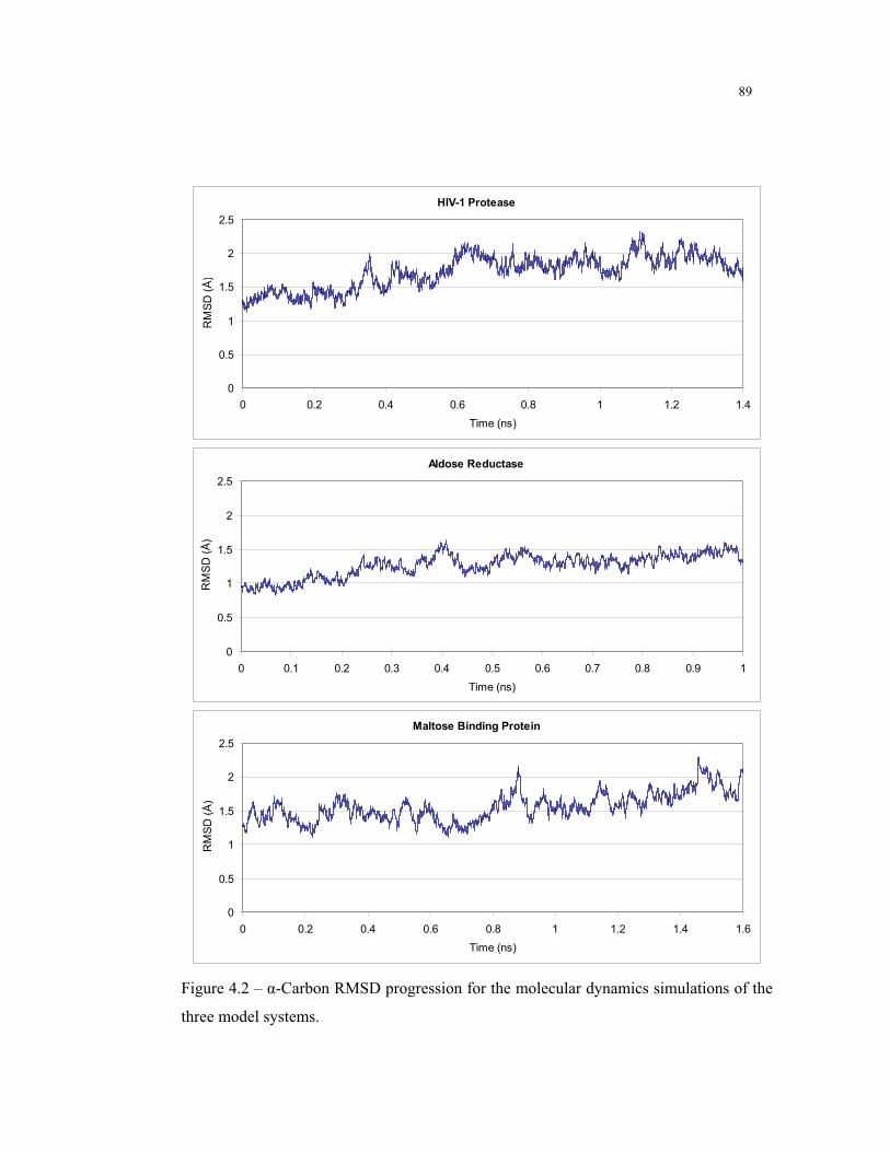
89

HIV-1 Protease

0

0.5

1

1.5

2

2.5

0 0.2 0.4 0.6 0.8 1 1.2 1.4

Time (ns)

RM

SD

(Å

)

Aldose Reductase

0

0.5

1

1.5

2

2.5

0 0.1 0.2 0.3 0.4 0.5 0.6 0.7 0.8 0.9 1

Time (ns)

RM

SD

(Å

)

Maltose Binding Protein

0

0.5

1

1.5

2

2.5

0 0.2 0.4 0.6 0.8 1 1.2 1.4 1.6

Time (ns)

RM

SD

(Å

)

Figure 4.2 – -Carbon RMSD progression for the molecular dynamics simulations of the

three model systems.

90

The RMS deviations versus the original crystal structure during the production

part of the simulation are shown in Figure 4.2. The plots show that all proteins are

stable during the simulation period. The average RMSD values for the first 100 ps of

simulation are 1.351 Å, 0.948 Å, and 1.405 Å for HIV-1 protease, aldose reductase, and

maltose binding protein, respectively. The same values for the last 100 ps of simulation

are 1.837 Å, 1.454 Å, and 1.849 Å. The overall level of conformational variation is

approximately the same for all protein systems. The change in conformation that is

observed for proteins is not due to simulation instability and is within the ranges

normally observed for these types of simulations.

The RMSD changes shown in Figure 4.2 during the simulation correspond in

large part to changes at the level of the binding site. However, this information is not

clearly observable just by visualizing the output of the simulation. Although, especially

for the case of HIV-1 protease, it is possible to observe by visualization of the raw data

a larger flexibility component at the level of the binding site, this is not immediately

clear for the other two cases. This is the main reason why we decided to use a

dimensional reduction methodology in the present work. The purpose of this technique

is to help understand what the most important components of protein flexibility are. In

addition the PCA method provides us with an abstract and compact flexibility

representation that enables the use of its results in modeling studies such as structure-

based drug design.

91

4.4.2. Backbone PCA

One of the advantages of the dimensional reduction method using PCA is the

ability to carry out the data analysis at different levels of detail and focusing on

different parts of the protein. Although an analysis consisting of all the atoms in the

protein provides us with information regarding all levels of detail, such as backbone or

binding site, it is also computationally more expensive and often unnecessary. In this

section we will analyze the results of studying the flexibility of the protein at the

backbone level. In this computation we included as part of the backbone atoms the N,

CA, and C atoms. The O, HN, and H were not included because their positions can be

readily approximated from the other three. Alternatively, we could have chosen to

represent the backbone using only the CA atoms. The backbone representation chosen

for this study uses 9 degrees of freedom per aminoacid. As such the total number of

degrees of freedom is 1782 for HIV-1 protease, 2835 for aldose reductase, and 3330 for

maltose binding protein. If we had used all the atoms in the proteins these numbers

would have been 9360, 15732, and 17211, respectively.

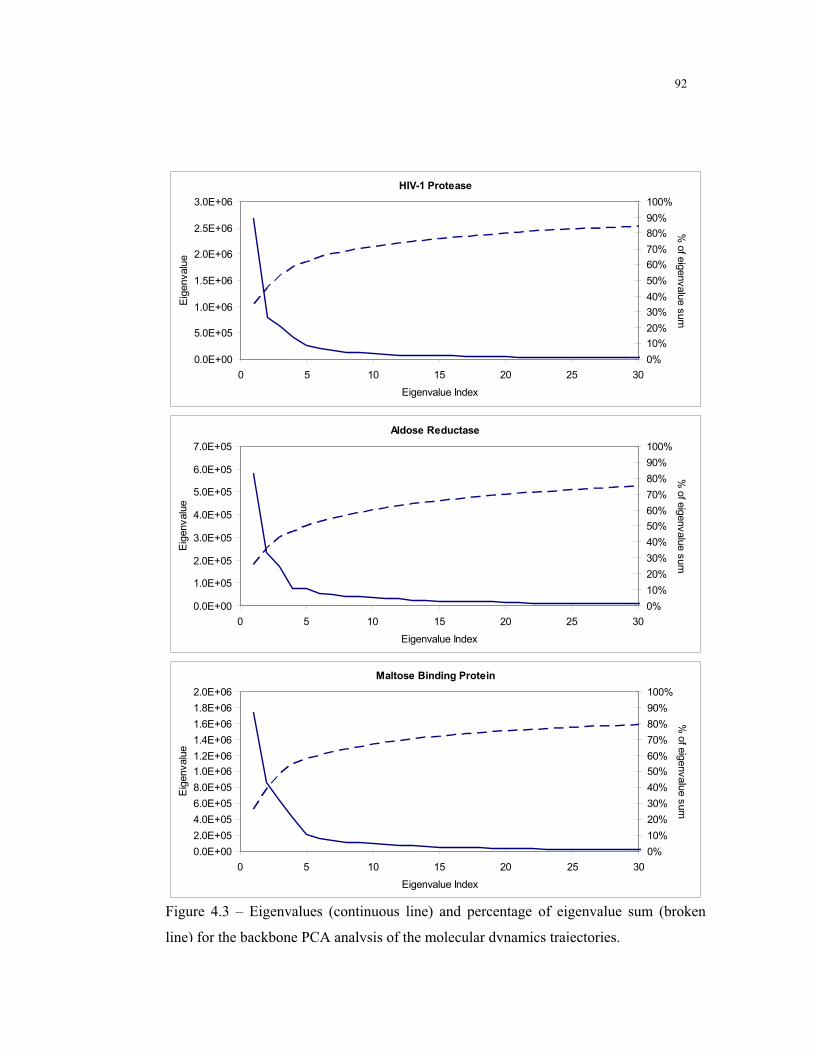
92

HIV-1 Protease

0.0E+00

5.0E+05

1.0E+06

1.5E+06

2.0E+06

2.5E+06

3.0E+06

0 5 10 15 20 25 30

Eigenvalue Index

Eig

env

alu

e

0%

10%

20%

30%

40%

50%

60%

70%

80%

90%

100%

% of eigen

value su

m

Aldose Reductase

0.0E+00

1.0E+05

2.0E+05

3.0E+05

4.0E+05

5.0E+05

6.0E+05

7.0E+05

0 5 10 15 20 25 30

Eigenvalue Index

Eig

enval

ue

0%

10%

20%

30%

40%

50%

60%

70%

80%

90%

100%

% of e

igenv

alue sum

Maltose Binding Protein

0.0E+00

2.0E+05

4.0E+05

6.0E+05

8.0E+05

1.0E+06

1.2E+06

1.4E+06

1.6E+06

1.8E+06

2.0E+06

0 5 10 15 20 25 30

Eigenvalue Index

Eig

enva

lue

0%

10%

20%

30%

40%

50%

60%

70%

80%

90%

100%

% o

f eigenva

lue sum

Figure 4.3 – Eigenvalues (continuous line) and percentage of eigenvalue sum (broken

line) for the backbone PCA analysis of the molecular dynamics trajectories.

93

The eigenvalues for the PCA analysis of the three protein models are plotted

using a continuous line in Figure 4.3. The absolute values for the eigenvalues are shown

on the left axis. The right axis and the broken line indicate the percentage of the

eigenvalue sum contributed by the eigenvalues with index less than or equal to the

current index. Only the largest 30 eigenvalues are plotted. All the proteins in this study

displayed a significant eigenvalue drop with the first few eigenvalues accounting for

most of the eigenvalue sum. For the case of HIV-1 protease the first, second, and third

eigenvalues account for 34.8%, 45.2%, and 53.2% of the eigenvalue sum. These

numbers illustrate the power of the dimensional reduction method. Using only 0.17% of

the initial number of degrees of freedom in the system, it is possible to account for

more than half of the variance observed during a molecular simulation for this

particular system. For the case of aldose reductase the first, second, and third

eigenvalues account for 25.6%, 35.8%, and 43.4%. The same numbers for maltose

binding protein are 26.1%, 39.0%, and 48.6%, respectively. These numbers are similar

to the ones obtained for HIV-1 protease but the differences are relevant. The first aspect

to note is that the values for aldose reductase are smaller. This can be explained by the

reduced flexibility of this protein in comparison to the other two. HIV-1 protease and

especially maltose binding protein undergo large conformational changes upon ligand

binding (see Appendix A. for details). In contrast, aldose reductase undergoes little or

almost no conformations changes depending on the ligand. Furthermore, this changes

happen almost exclusively at the binding site level with the rest of the protein

remaining almost unchanged. This difference in overall flexibility can be also observed

94

from the absolute values of the eigenvalues. The sums of the first three eigenvalues for

HIV-1 protease, aldose reductase, and maltose binding protein are 4.09×107, 9.88×10

6,

and 3.24×107, respectively. Another important difference is the ratio between the first

eigenvalues for the three systems. Whereas for HIV-1 protease, the first eigenvalue

clearly dominates the eigenvalue spectrum, for the other proteins there is a more

gradual drop in eigenvalues. The ratios between the first and second eigenvalues for

HIV-1 protease, aldose reductase, and maltose binding protein are 3.35, 2.50, and 2.02,

respectively. These values are of great importance when later we examine the motions

corresponding to these eigenvalues. On one hand, due to the large dominance of the

first eigenvalue, the first eigenvector for HIV-1 protease can represent a good

approximation to a relevant biological motion for this protein. On the other hand, the

small difference in first and second eigenvalues for maltose binding protein precludes

the interpretation of the first mode of motion for this protein without consideration of

the second.

95

Figure 4.4 – First mode of motion for the backbone of HIV-1 protease. The backbone is

colored from red to blue as a function of the residue number. a) Stereoview of the

mapping of the first eigenvector on the C- atoms. The directions of motions are

indicated by purple arrows. b) Changes in conformation corresponding to a motion in

both directions along the first mode of motion starting from the experimental structure

(center).

96

In the dimensional reduction method using PCA, there is an eigenvector

corresponding to each eigenvalue. The eigenvalues provide information about the

number of relevant motions and their relative importance. The eigenvectors can be

mapped back to the structure of the protein to indicate directions of preferred motion.

Given a 3N dimensional eigenvector, corresponding to the N atoms in the protein for

which the PCA analysis was carried out, the motions can be readily visualized by

partitioning the eigenvector into N Cartesian vectors and mapping each of these to its

corresponding atom. Figure 4.4 shows the mapping of the first eigenvector to the

backbone of HIV-1 protease. This corresponds to the first mode of motion. The

direction of motion is indicated in Figure 4.4 - a) by the Cartesian vectors (purple

arrows) for each CA atom. The arrows corresponding to the N and C atom motions

were omitted for clarity. The length of the arrows indicates the relative amount of

motion for each CA atom. Figure 4.4 - b) shows conformational changes corresponding

to a motion in both directions along the first mode of motion starting from the

experimental structure. The motion is exaggerated for illustration purposes. The first

mode of motion for HIV-1 protease is in excellent accordance to the experimental data

available for this protein. The motion occurs mostly in the flaps region and clearly

indicates an opening of the flaps in order to expose the binding site. The motion also

suggests a transition path between the bound and unbound experimental structures and

between alternative bound forms (see Appendix A.1.). For example, the structure

shown on the left side of Figure 4.4 - b) is similar to the unbound conformation of HIV-

1 protease (Wlodawer, Miller et al. 1989) and to other bounds forms such as 1AID

97

(Rutenber, Fauman et al. 1993) shown in Figure A.2. The motion is also in good

agreement with previous simulation studies using molecular dynamics (Collins, Burt et

al. 1995). The mapping of the first eigenvector to the protein structure also shows a

significant amount of motion at the level of the 78-83 loop near the binding site. This

loop has been shown to undergo significant conformation changes during binding of

some HIV-1 protease inhibitors (Munshi, Chen et al. 2000). The core of the protein

stays mostly unchanged according to the first mode of motion. This is also in good

agreement with the available experimental structures for HIV-1 protease, which show

much less conformational variation at the core than at the binding site level.

The second mode of motion for HIV-1 protease is shown in Figure 4.5. This

mode is complementary to the first and also explains conformational rearrangements

that HIV-1 undergoes when binding to different ligands. While the first mode

corresponds to an opening of the flaps region and therefore a change in binding site

volume mostly in that direction, the second mode corresponds to a sideways

constriction of the binding site allowing for variations in the width of the ligand. Unlike

the first mode, there is less variation in the relative size of the arrows. The motion is not

restricted to a particular site on the protein but is mostly a change in the relative

orientation of the two protein monomers leading to a loosening/tightening of the

binding site (see Figure 4.5 – b) left and right).

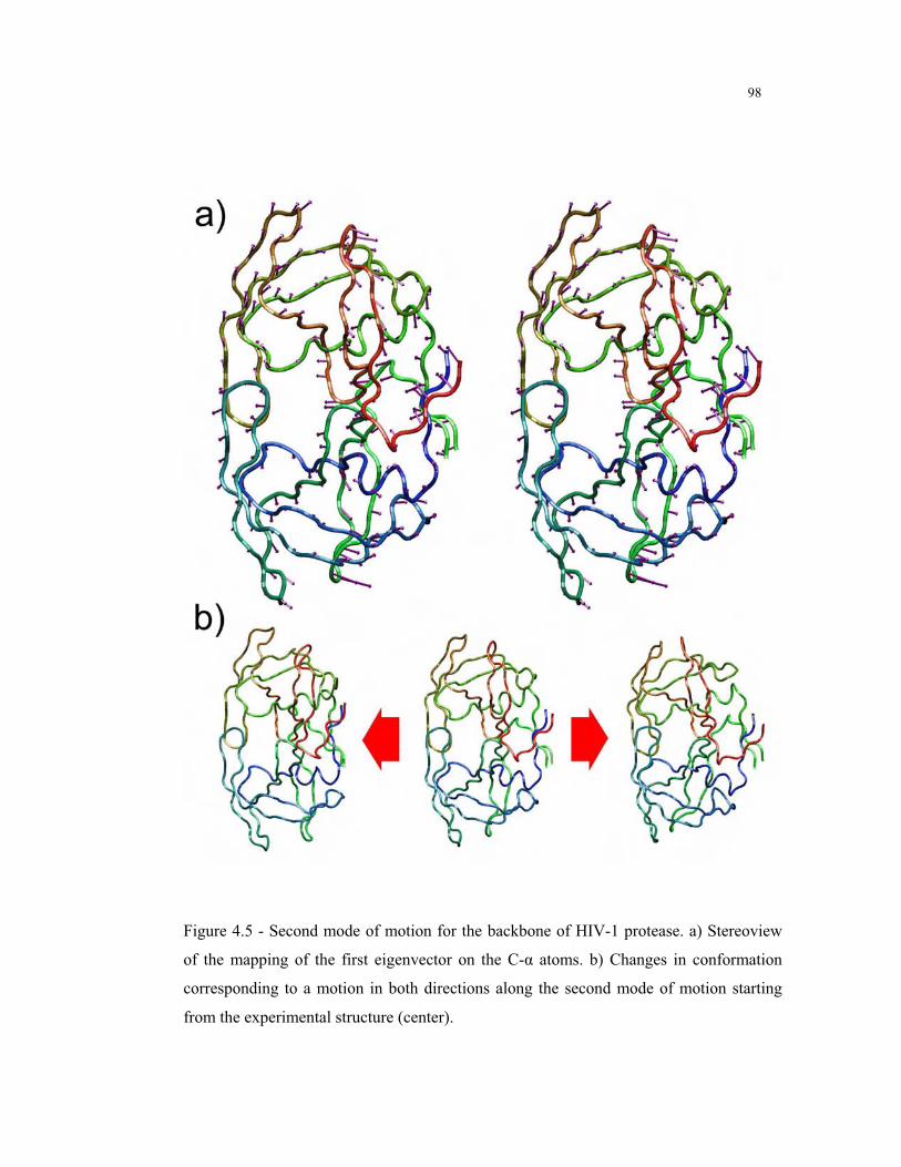
98

Figure 4.5 - Second mode of motion for the backbone of HIV-1 protease. a) Stereoview

of the mapping of the first eigenvector on the C- atoms. b) Changes in conformation

corresponding to a motion in both directions along the second mode of motion starting

from the experimental structure (center).

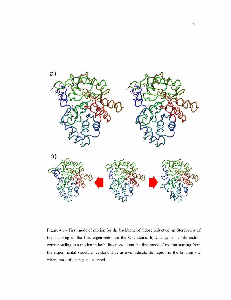
99

Figure 4.6 - First mode of motion for the backbone of aldose reductase. a) Stereoview of

the mapping of the first eigenvector on the C- atoms. b) Changes in conformation

corresponding to a motion in both directions along the first mode of motion starting from

the experimental structure (center). Blue arrows indicate the region in the binding site

where most of change is observed.

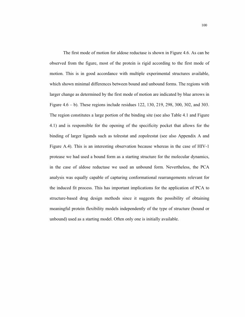
100

The first mode of motion for aldose reductase is shown in Figure 4.6. As can be

observed from the figure, most of the protein is rigid according to the first mode of

motion. This is in good accordance with multiple experimental structures available,

which shown minimal differences between bound and unbound forms. The regions with

larger change as determined by the first mode of motion are indicated by blue arrows in

Figure 4.6 – b). These regions include residues 122, 130, 219, 298, 300, 302, and 303.

The region constitutes a large portion of the binding site (see also Table 4.1 and Figure

4.1) and is responsible for the opening of the specificity pocket that allows for the

binding of larger ligands such as tolrestat and zopolrestat (see also Appendix A and

Figure A.4). This is an interesting observation because whereas in the case of HIV-1

protease we had used a bound form as a starting structure for the molecular dynamics,

in the case of aldose reductase we used an unbound form. Nevertheless, the PCA

analysis was equally capable of capturing conformational rearrangements relevant for

the induced fit process. This has important implications for the application of PCA to

structure-based drug design methods since it suggests the possibility of obtaining

meaningful protein flexibility models independently of the type of structure (bound or

unbound) used as a starting model. Often only one is initially available.

101

Figure 4.7 - First mode of motion for the backbone of maltose binding protein. a)

Stereoview of the mapping of the first eigenvector on the C- atoms. b) Changes in

conformation corresponding to a motion in both directions along the first mode of motion

starting from the experimental structure (center).

102

The first mode of motion for maltose binding protein is shown in Figure 4.7. As

can be observed from Figure 4.7 – a) the hinge bending motion that characterizes the

conformational transition between the bound and unbound forms of this protein is not

clearly observable. Even though there are no intra domain movements in the top and

bottom domains (top domain shown mostly in red, yellow, and blue on the top of

Figure 4.7 – a) and bottom domain shown mostly in green at the bottom of the figure)

which would be indicated by large arrows pointing to mostly different directions within

the same domain, there is a clear twisting motion of one domain relative to the other

that leads to a moderate opening/closing of the binding site region (see Figure 4.7 – b)

). This result was a clear reminder that modes derived from PCA cannot be interpreted

by themselves as real modes of protein motion: what they constitute is a reduced

dimensional basis for representing motions of proteins. Real protein motion may be a

result of the combination of two or more of the PCA modes. As discussed before, one

of the main differences between the results of HIV-1 protease and maltose binding

protein is the ratio between the first and second eigenvectors. While for HIV-1 protease

there is a clear dominance of the first mode in the eigenvalue spectrum, for maltose

binding protein there is a much small difference between the first and second modes.

As a result, it is important for the case of maltose binding protein to also look at the

mode corresponding to the second largest eigenvalue and determine how a combination

of the two can result in experimentally observed protein motions. Observation of the

second mode of motion revealed a particularly interesting result. The second mode also

consists of a twist of one domain relative to the other but in the opposite direction. The

103

motion is equally accompanied by a moderate opening/closing motion about the hinge

position near the binding site. The motions are illustrated in Figures 4.8 and 4.9 (note:

the figures are stereoviews and should be viewed in portrait mode by looking up and

down to give the illusion of motion). The figures are color coded according to the

respective collective motion. Red is used for the first mode of motion and blue is used

for the second. On Figure 4.8 the motion is for the molecule in red and the blue

structure corresponds to the original conformation. On Figure 4.9 the motion is for the

molecule in blue using the red conformation as a reference. The first mode corresponds

to a counterclockwise rotation of the top domain in relation to the bottom domain

(relative dispositions as shown in the figure) around the axis defined by the red arrows.

Conversely, the second mode corresponds to a clockwise rotation. Both modes lead to

simultaneous opening or closing as they twist in opposite directions. By considering the

two modes in conjunction it is possible to obtain an opening and closing of the binding

site of maltose binding protein which does not occur in a straight direction but instead

takes place in a zigzag motion. Given the results of the PCA analysis this is presently

our model for the biologically relevant motion of this protein. Unfortunately, it is not

currently possible to experimentally prove or refute this model.

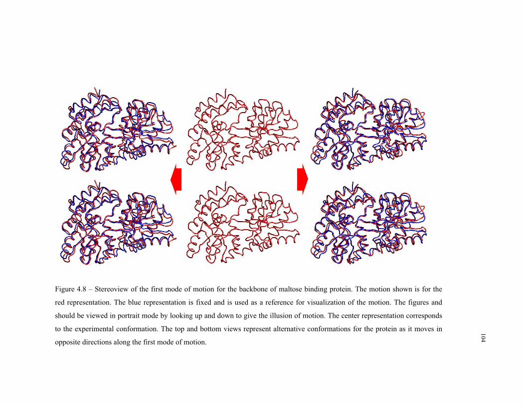
104

Figure 4.8 – Stereoview of the first mode of motion for the backbone of maltose binding protein. The motion shown is for the

red representation. The blue representation is fixed and is used as a reference for visualization of the motion. The figures and

should be viewed in portrait mode by looking up and down to give the illusion of motion. The center representation corresponds

to the experimental conformation. The top and bottom views represent alternative conformations for the protein as it moves in

opposite directions along the first mode of motion.

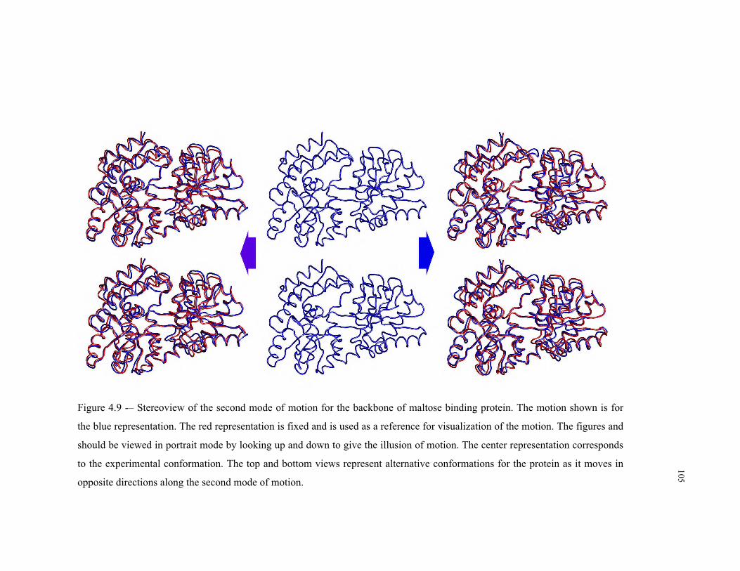
105

Figure 4.9 -– Stereoview of the second mode of motion for the backbone of maltose binding protein. The motion shown is for

the blue representation. The red representation is fixed and is used as a reference for visualization of the motion. The figures and

should be viewed in portrait mode by looking up and down to give the illusion of motion. The center representation corresponds

to the experimental conformation. The top and bottom views represent alternative conformations for the protein as it moves in

opposite directions along the second mode of motion.

106

Another useful piece of information that can be obtained by carrying out the

PCA calculation using the singular value decomposition method is the right singular

vectors. The right singular vectors correspond to the reduced coordinate representation

in the new basis defined by the left singular vectors. In other words, it is the reduced set

of coordinates that represents the original protein motion. For the case of molecular

dynamics data, the analysis of this set reveals a set of stable conformational substates

that correspond to local energy minima in the conformational energy landscape of the

protein. The two and three dimensional plots of the right singular vectors have been

previously described as “beads-on-a-string”. The beads correspond to low energy

regions with long residence times and the string connecting the beads corresponds to

fast transitions between metastable substates. For an extensive discussion on the

identification and modeling of protein conformational substates see Romo’s thesis

(Romo 1998).

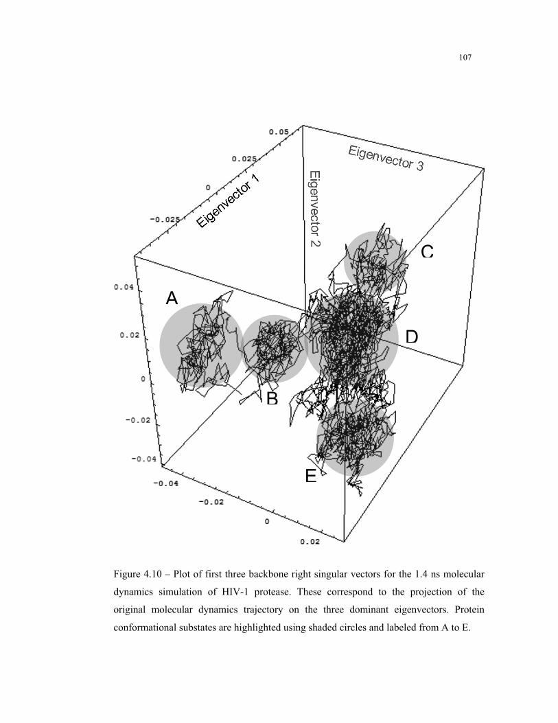
107

Figure 4.10 – Plot of first three backbone right singular vectors for the 1.4 ns molecular

dynamics simulation of HIV-1 protease. These correspond to the projection of the

original molecular dynamics trajectory on the three dominant eigenvectors. Protein

conformational substates are highlighted using shaded circles and labeled from A to E.

A

B

C

D

E

108

Figure 4.10 shows the plot of first three right singular vectors. These correspond

to the projection of the original molecular dynamics trajectory on the three dominant

eigenvectors. The plot shows a three dimensional scatter plot in which consecutive

points in time are connected by straight lines. In the case of HIV-1 protease 2800 points

are plotted in Figure 4.10. As a result each straight line connecting two points

corresponds to 5 ps of simulation. It is possible that if we had used a finer time

sampling we would observe even more structure in the plots. Such observation would

be consistent with the current hierarchical view of ensembles of substates in which each

substate can be further divided into another ensemble of substates corresponding to

smaller conformational changes. The results show that during the simulation the protein

does not change its conformation continuously from the beginning to the end of the

simulation but instead jumps between conformational substates. Protein conformational

substates are highlighted using shaded circles and labeled from A to E. These

correspond to the following approximate time periods: A from 0 ps to 150 ps, B from

150 ps to 325 ps, C from 325 ps to 600 ps, D from 600 ps to 900 ps, and E from 900 ps

to 1400 ps. The information obtained from the right singular vectors is also relevant for

structure-based drug design because it can hint at certain protein conformations that are

more stable in solution and as such should be targeted preferentially in a virtual

screening study. This kind of approach allows the use of the power of dimensional

reduction methods to include protein flexibility in the drug design process without a

large increase in computational expense. This method is going to be explored further in

109

Chapter 5 when we discuss possible uses of the dimensional reduction methodology in

drug design applications.

In order to check if the protein conformational substates correspond in fact to

similar backbone conformations we also calculated pairwise backbone RMSD values

for the entire trajectory. If this is the case we should see squares of lower RMSD value

along the diagonal of the pairwise RMSD matrix. Figure 4.11 shows the backbone

RMSD matrix for the 1.4 ns molecular dynamics simulation of HIV-1 protease. The

two axes represent 1400 backbone structures sampled every 10 ps. In this plot we can

unmistakably verify the existence of the first three conformational substates labeled A,

B, and C. The distinctions between substates D and E is not as clearly defined. This

reflects the fact than in Figure 4.10, states D and E are close together in the reduced

space and there seems to be a lot of interconversion between these. In contrast there is a

very clear transition between states A and B with a single path (line) connecting the two

states without any interconversion. The comparison of the two plots suggests that

analysis of right singular vectors is a better method to identify protein conformational

substates.

110

Figure 4.11 – Backbone RMSD matrix for the 1.4 ns molecular dynamics simulation of

HIV-1 protease. The two axis represent 1400 backbone structures sampled every 10 ps.

The RMSD value between two structures is represented off the diagonal at the

intersection of the respective indices (note: the data on the two side of the diagonal is

identical). Protein conformational substates identified using Figure 4.10 are labeled from

A to E.

A

B

C

D

E

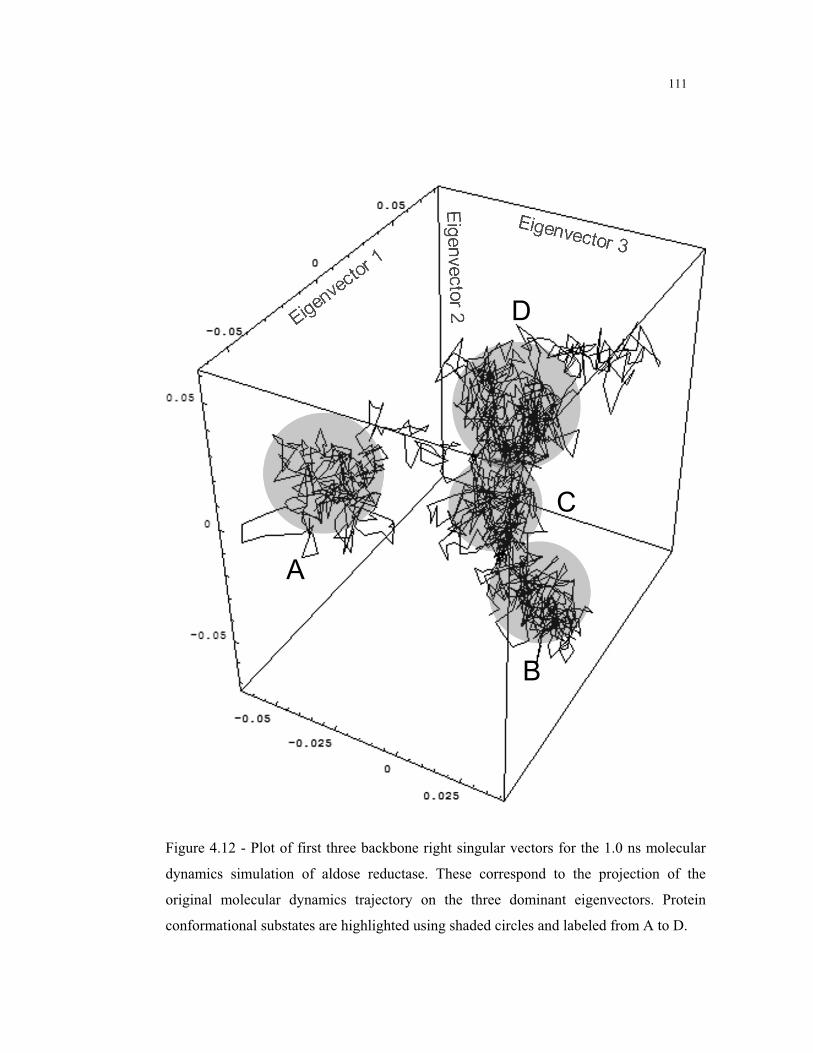
111

Figure 4.12 - Plot of first three backbone right singular vectors for the 1.0 ns molecular

dynamics simulation of aldose reductase. These correspond to the projection of the

original molecular dynamics trajectory on the three dominant eigenvectors. Protein

conformational substates are highlighted using shaded circles and labeled from A to D.

A

B

C

D

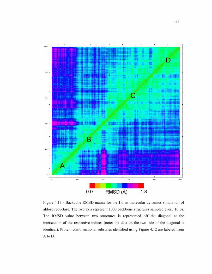
112

Figure 4.13 - Backbone RMSD matrix for the 1.0 ns molecular dynamics simulation of

aldose reductase. The two axis represent 1000 backbone structures sampled every 10 ps.

The RMSD value between two structures is represented off the diagonal at the

intersection of the respective indices (note: the data on the two side of the diagonal is

identical). Protein conformational substates identified using Figure 4.12 are labeled from

A to D.

A

B

C

D

113

Figure 4.12 shows the three main right singular vectors for the aldose reductase

trajectory. In this figure we can see a clearly isolated substate A that later migrates to

state B, which is much closer to the following states C and D. The same kind of

behavior can also be observed from Figure 4.13 where the conformations in state A are

markedly different from the three following substates. An alternative interpretation for

this result is to use the hierarchical model and consider only two substates X and Y. X

would be composed only of the state A, and Y could be further decomposed in states B,

C and D.

Figure 4.14 shows the three main right singular vectors for the maltose binding

protein trajectory. The plot visibly isolates three conformational substates labeled A to

C. However, when we compare this data to the pairwise RMSD plots in Figure 4.15

these substates cannot be readily identified. This is a case where the right singular

vectors are clearly more powerful in the identification of conformational substates.

114

Figure 4.14 - Plot of first three backbone right singular vectors for the 1.6 ns molecular

dynamics simulation of maltose binding protein. These correspond to the projection of

the original molecular dynamics trajectory on the three dominant eigenvectors. Protein

conformational substates are highlighted using shaded circles and labeled from A to C.

A

B

C

115

Figure 4.15 - Backbone RMSD matrix for the 1.6 ns molecular dynamics simulation of

maltose binding protein. The two axis represent 2000 backbone structures sampled every

8 ps. The RMSD value between two structures is represented off the diagonal at the

intersection of the respective indices (note: the data on the two side of the diagonal is

identical). Protein conformational substates identified using Figure 4.14 are labeled from

A to C.

A

B

C

116

4.4.3. Binding Site PCA

Changes at the level of the binding site are the most critical in determining the

binding of a ligand to the receptor protein. In this section we focused the dimensional

reduction analysis on the residues that constitute the binding site (see Figure 4.1). The

main advantage from a structure-based drug design point of view in considering only

the binding site atoms in the PCA calculation is to avoid the inclusion of motions that

are not relevant for ligand binding in the main modes of motion. If non-relevant atomic

motions were sufficiently large and well correlated they would mask the results

pertinent to induced fit effects at the level of the binding site. This problem will be

addressed in more detail in Chapter 5. A second advantage of using only binding site

atoms to calculate collective modes of motion for the protein is that, as in the case for

the backbone analysis, the initial dimension of the problem is already reduced. If we

consider the Cartesian degrees of freedom for each atom in the binding site, the initial

number of degrees of freedom is 750 for HIV-1 protease, 426 for aldose reductase, and

426 for maltose binding protein.

117

HIV-1 Protease

0.0E+00

2.0E+05

4.0E+05

6.0E+05

8.0E+05

1.0E+06

1.2E+06

1.4E+06

1.6E+06

1.8E+06

2.0E+06

0 5 10 15 20 25 30

Eigenvalue Index

Eig

enval

ue

0%

10%

20%

30%

40%

50%

60%

70%

80%

90%

100%

% o

f eig

envalu

e s

um

Aldose Reductase

0.0E+00

2.0E+04

4.0E+04

6.0E+04

8.0E+04

1.0E+05

1.2E+05

1.4E+05

1.6E+05

0 5 10 15 20 25 30

Eigenvalue Index

Eig

enva

lue

0%

10%

20%

30%

40%

50%

60%

70%

80%

90%

100%

% of e

igenva

lue su

m

Maltose Binding Protein

0.0E+00

5.0E+04

1.0E+05

1.5E+05

2.0E+05

2.5E+05

3.0E+05

0 5 10 15 20 25 30

Eigenvalue Index

Eig

enva

lue

0%

10%

20%

30%

40%

50%

60%

70%

80%

90%

100%

% o

f eigenv

alue

sum

Figure 4.16 - Eigenvalues (continuous line) and percentage of eigenvalue sum (broken

line) for the binding site PCA analysis of the molecular dynamics trajectories.

118

The eigenvalues and eigenvalue sums for the binding site PCA analysis of the

three protein models are shown in Figure 4.16. As in the case of the backbone analysis,

all the proteins in this study displayed a significant eigenvalue drop with the first few

eigenvalues accounting for most of the eigenvalue sum. For the case of HIV-1 protease

the first, second, and third eigenvalues account for 43.6%, 53.0%, and 58.9% of the

eigenvalue sum. For the case of aldose reductase the first, second, and third eigenvalues

account for 27.0%, 38.6%, and 49.4%. The same numbers for maltose binding protein

are 23.0%, 36.4%, and 47.9%, respectively. In comparison with the backbone analysis

there is now a greater dominance of the main eigenvectors for the cases of HIV-1

protease and aldose reductase. The values for maltose binding protein are very similar

to the ones obtained for the binding site analysis. The larger change in results is for the

first two proteins because the changes on these proteins were mostly in the binding site

region. The changes for maltose binding protein are mainly a reorientation of domains.

In this case, the largest atomic displacements are far from the binding site region.

For the case of the binding site analysis, the right singular vectors can indicate

binding site conformations that are stable and should be used as target receptors in drug

design applications. In comparison with the right singular vectors obtained for the

backbone analysis, the ones derived from the binding site should display a cleaner

structure, which is easier to interpret. Figure 4.17 to 4.19 show the right singular vector

plots for the three proteins. The results for HIV-1 protease shown in Figure 4.17 are

comparable to the results shown in Figure 4.10. The first two conformational substates

A and B are common to both backbone and binding site analysis. Conformational

119

substate C includes the backbone conformational substates C, D, and E. This indicates

that the changes that determined the transitions between these substates are not

determined by changes in the binding site. The results for aldose reductase shown in

Figure 4.18 are comparable to the results shown in Figure 4.12 and are similar to the

results obtained with HIV-1 protease. In this case there are only two major

conformational substates A and B. Conformational substate B corresponds to merging

states B, C, and D. The results for maltose binding protein shown in Figure 4.19 also

show three conformational substates as in Figure 4.14. However the residence time in

state B is shorter than in the case of the backbone analysis.

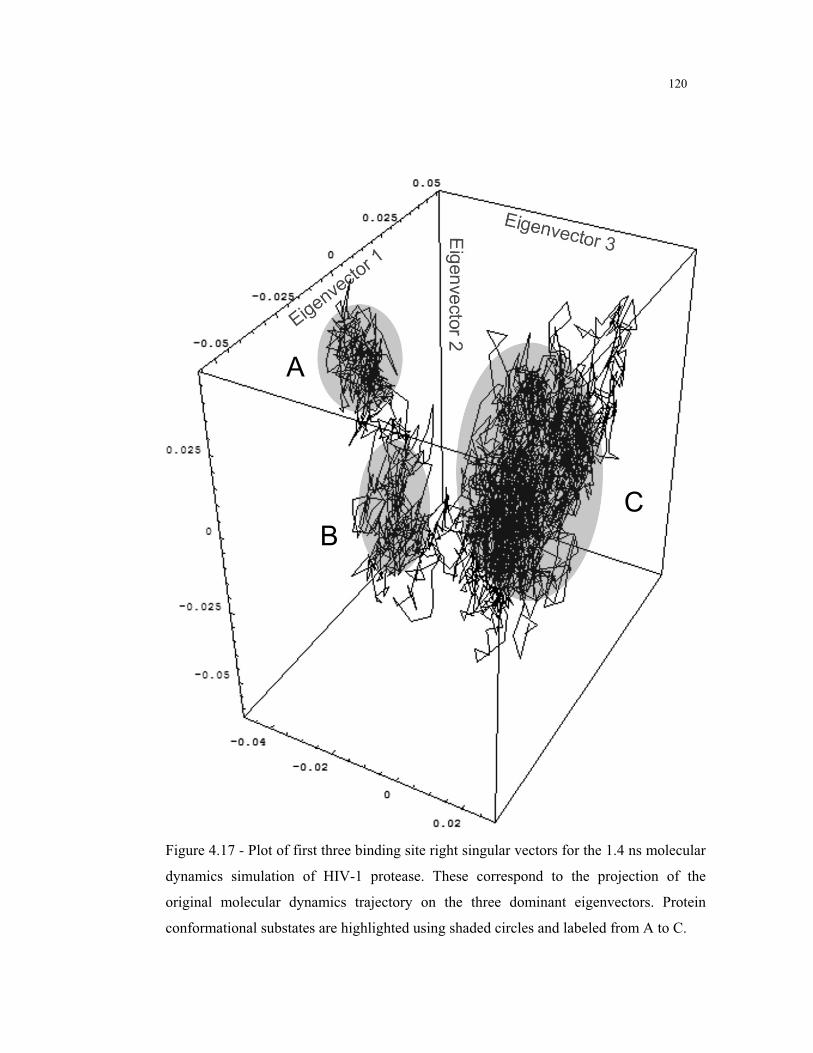
120

Figure 4.17 - Plot of first three binding site right singular vectors for the 1.4 ns molecular

dynamics simulation of HIV-1 protease. These correspond to the projection of the

original molecular dynamics trajectory on the three dominant eigenvectors. Protein

conformational substates are highlighted using shaded circles and labeled from A to C.

A

BC

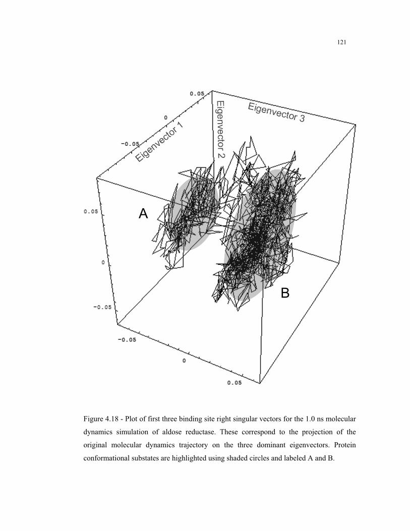
121

Figure 4.18 - Plot of first three binding site right singular vectors for the 1.0 ns molecular

dynamics simulation of aldose reductase. These correspond to the projection of the

original molecular dynamics trajectory on the three dominant eigenvectors. Protein

conformational substates are highlighted using shaded circles and labeled A and B.

A

B

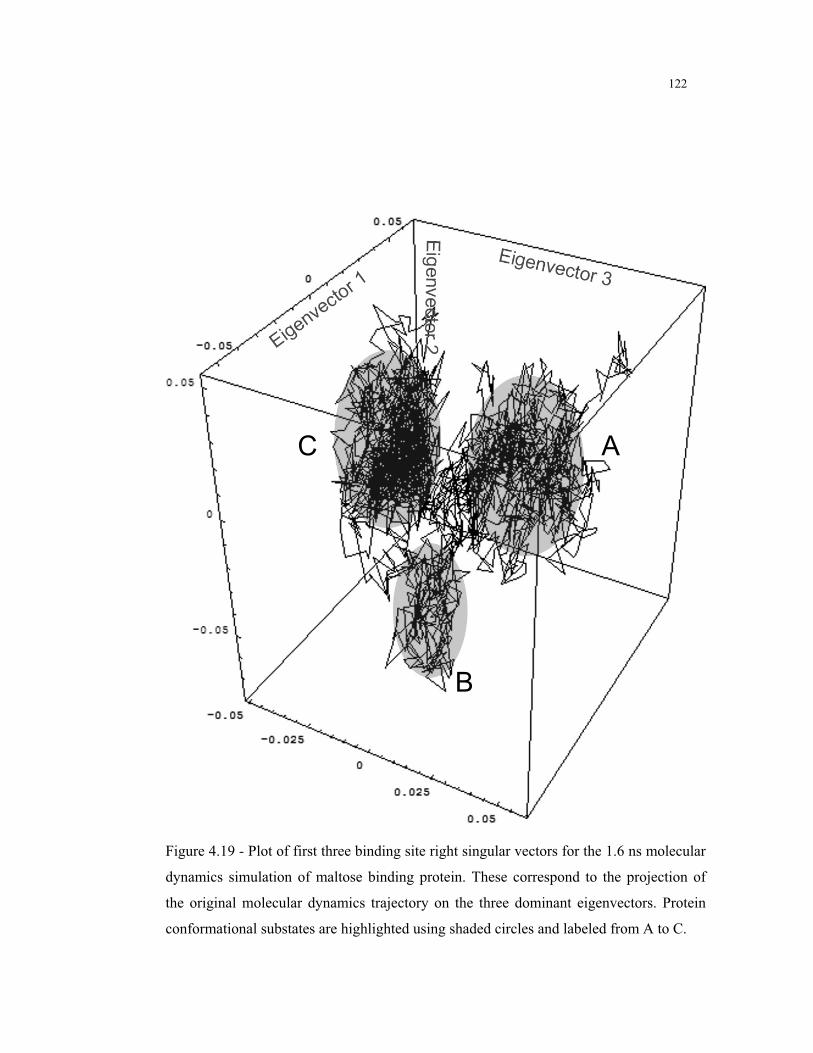
122

Figure 4.19 - Plot of first three binding site right singular vectors for the 1.6 ns molecular

dynamics simulation of maltose binding protein. These correspond to the projection of

the original molecular dynamics trajectory on the three dominant eigenvectors. Protein

conformational substates are highlighted using shaded circles and labeled from A to C.

A

B

C

123

4.4.4. All-Atoms PCA

The final level of detail we tested using the PCA method was to include all the

atoms in the protein in the calculation. Due to the increase computational requirements

for this computation it was carried out only for HIV-1 protease. The computation of the

PCA for all atoms of HIV-1 protease has the following memory requirements. The

initial data consists of 14,000 data points for 9360 degrees of freedom. Each data point

is a single precision floating point number (4 bytes on a 32 bit machine). As a result the

initial data occupies approximately 500 MB (megabyte). This data is used for the

computation of the covariance matrix of size 9360 by 9360. In order to increase

numerical stability, the covariance matrix is computed using double precision floating

point numbers (8 bytes on a 32 bit machine). The covariance matrix has size

approximately 670 MB. Due to bad memory management, the program Mathematica

uses approximately four times more memory than what is theoretically required. As a

result, the all-atoms PCA computation is not practical using this program because we

did not have access to a computer with the required specifications. The use of swap

space on hard disk to increase the available virtual memory is also not practical due to

the very high latency of accessing the data from hard disk when compared to physical

memory or CPU cache. Although using swap space as an alternative solution is

possible, it increases the computation time by approximately two orders of magnitude.

By reason of the limitations described above we developed the program svd that can

efficiently manage memory and carry out the above computation on machines with

approximately 1 GB (gigabye) of memory. The program is also capable of adapting to

124

smaller physical memory sizes by carrying out matrix computations, such as

vector/vector multiplications, in blocks.

The eigenvalues and eigenvalue sums for the all-atoms PCA analysis of the

HIV-1 protease is shown in Figure 4.20. As in the case of the backbone and binding site

analyses, we observed a significant eigenvalue drop, with the first few eigenvalues

accounting for most of the eigenvalue sum. The first, second, and third eigenvalues

account for 19.4%, 29.0%, and 36.2% of the eigenvalue sum. The numbers are smaller

than for the cases of the backbone and binding site analyses but the total number of

degrees of freedom is also much larger (9360 versus 1782 and 750, respectively). Based

on visual inspection, the first mode of motion determined for all-atoms is similar to the

one calculated for the backbone (result not shown). The motion also corresponds to an

opening/closing of the binding site but with extra information regarding aminoacid

sidechain positions.

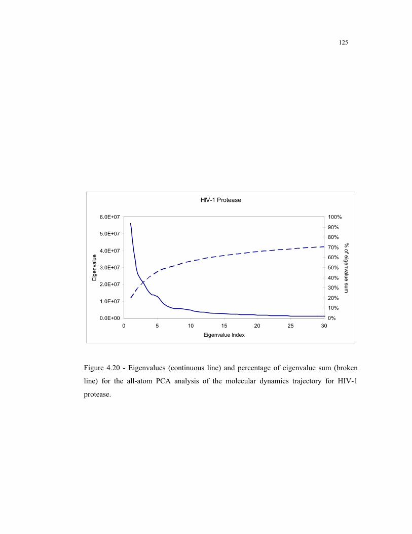
125

HIV-1 Protease

0.0E+00

1.0E+07

2.0E+07

3.0E+07

4.0E+07

5.0E+07

6.0E+07

0 5 10 15 20 25 30

Eigenvalue Index

Eig

en

valu

e

0%

10%

20%

30%

40%

50%

60%

70%

80%

90%

100%

% o

f eig

en

valu

e su

m

Figure 4.20 - Eigenvalues (continuous line) and percentage of eigenvalue sum (broken

line) for the all-atom PCA analysis of the molecular dynamics trajectory for HIV-1

protease.

126

4.4.5. PCA analysis of experimental structures

In order to validate the results obtained from the PCA analysis of the molecular

dynamics data we performed the same type of mathematical analysis for the

experimental data obtained using X-ray crystallography. Comparisons done between

traditional molecular simulations and experimental techniques (Clarage, Romo et al.

1995; Philippopoulos and Lim 1999) seem to indicate that X-ray crystallography and

NMR structures provide better coverage of conformational spaces. As such modes

derived using experimental data should also provide a better representation of protein

flexibility. Unfortunately, the PCA analysis requires the availability of a large number

of conformations in order to calculate accurate correlation coefficients between the

initial degrees of freedom of the protein system. The use of experimental data for the

purposes of dimensional reduction is therefore limited to a handful of protein systems

for which there is a large number of experimentally derived structures available.

Although of limited applicability, this test allows a comparison of the results based on

computational data to results based purely on experimental data. For this purpose we

superimposed 134 structures of HIV-1 protease to the structure determined by Miller et

al (Miller, Schneider et al. 1989) (see Apendix B. for full list of structures) and

extracted the relevant backbone coordinate information to construct matrix A (see

section 4.3.3). The results obtained for the eigenvalue spectrum are similar to those

obtained when computationally derived data was used (see Figure 4.3). The first 3 and

first 20 eigenvalues account for 59% and 85% of the total eigenvalue sum, respectively.

These values are slightly higher than for the backbone analysis of the molecular

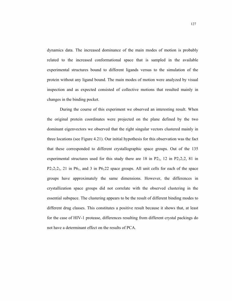
127

dynamics data. The increased dominance of the main modes of motion is probably

related to the increased conformational space that is sampled in the available

experimental structures bound to different ligands versus to the simulation of the

protein without any ligand bound. The main modes of motion were analyzed by visual

inspection and as expected consisted of collective motions that resulted mainly in

changes in the binding pocket.

During the course of this experiment we observed an interesting result. When

the original protein coordinates were projected on the plane defined by the two

dominant eigenvectors we observed that the right singular vectors clustered mainly in

three locations (see Figure 4.21). Our initial hypothesis for this observation was the fact

that these corresponded to different crystallographic space groups. Out of the 135

experimental structures used for this study there are 18 in P21, 12 in P21212, 81 in

P212121, 21 in P61, and 3 in P6122 space groups. All unit cells for each of the space

groups have approximately the same dimensions. However, the differences in

crystallization space groups did not correlate with the observed clustering in the

essential subspace. The clustering appears to be the result of different binding modes to

different drug classes. This constitutes a positive result because it shows that, at least

for the case of HIV-1 protease, differences resulting from different crystal packings do

not have a determinant effect on the results of PCA.

128

-5

-4

-3

-2

-1

0

1

2

3

4

5

6

7

8

-5 -4 -3 -2 -1 0 1 2 3 4 5 6 7 81st eigenvector

2nd

eig

enve

ctor

Figure 4.21 - Projection of coordinate vectors of 135 experimental HIV-1 protease

structures on the plane defined by the two dominant eigenvectors of the PCA. The circles

indicate clustering of structures in the essential subspace.

129

Although the type of procedure described above using experimental data

exclusively is more representative of the conformational flexibility of the model protein

when binding to inhibitors of different shapes, it also has several shortcomings. The

most important limitation of this approach is that for almost all systems for which

determining the main modes of protein flexibility would be beneficial there is not

enough experimental data to calculate an accurate correlation matrix. Due to its clinical

importance HIV-1 protease is currently a unique case of having a large number of

experimentally determined structures. Nevertheless, even the use of 135 experimental

structures is likely to introduce a large error. This problem has been analyzed by Genest

(Genest 1999) who observed that accurate correlation results could be obtained by

using approximately 2000 experimental points for 20 atoms. When the number of

experimental samples decreased, the number of false correlations observed increased.

In this calculation I used a higher number of atoms (198) and a smaller number of

experimental points (135). This is also likely to lead to the observation of correlations

that are not present in reality. A second limitation of using experimental data is that we

are biasing the conformational space sampled by the main modes of motion to reflect

only the binding modes that were already determined experimentally. If for example

there is a new binding mode corresponding to a novel class of drugs, the calculated

modes of flexibility would likely be of little help in discovering it in an hypothetical

flexible-protein / flexible-ligand database screening process. A possible method of

testing for errors in our experimental modes would be to a priori exclude part of our

experimental data from the dimensional reduction calculations and later check how well

130

the excluded data could be reproduced using the calculated modes of motion. The main

limitation to this test is again the reduced number of data available for the calculation of

the covariance matrix.

In order to determine the similarity between the modes of motion derived from

molecular dynamics data and the modes derived from experimental data we calculated

the overlap between the subspaces defined by the most significant principal

components. Overlap between two subspaces is calculated as the sum of all of the

squared inner products between all pairs of eigenvectors from both essential subspaces,

divided by the dimension of that space. When these projections are close to 1.0 for all

the eigenvectors of the subspace, the subspaces spanned by the two sets of eigenvectors

are the same. However, even if two subspaces are very similar it may happen that two

or more eigenvectors in one set are interchanged with respect to the other set resulting

in values lower than 1.0. In Figure 4.22 we show the cumulative inner products from

the projection of the molecular dynamics eigenvectors onto the first three eigenvectors

derived from experimental data. The eigenvectors for both structural sets were

calculated using C- data exclusively. As can be observed from the plot there is a

significant amount of overlap between the subspaces defined by the most significant

principal components. This result was also confirmed by visual inspection which

revealed similar motions for the first mode of motion. The results of this plot are similar

to what was previously observed for other proteins (van Aalten, Conn et al. 1997). In

this study, the authors compared the collective modes of motion derived from X-ray

crystallography experimental structures for eight different proteins. The results showed

131

significant overlap between the subspaces defined by the most significant principal

components. Differences between the modes derived by the different methods are

probably due to the following factors: 1) Incomplete sampling from the molecular

dynamics simulation (Clarage, Romo et al. 1995); 2) different protein environments

(solution vs. crystal); 3) insufficient number of structures used in the calculation of the

covariance matrix for the X-ray case; 4) limited variability in the ensemble of crystal

structures.

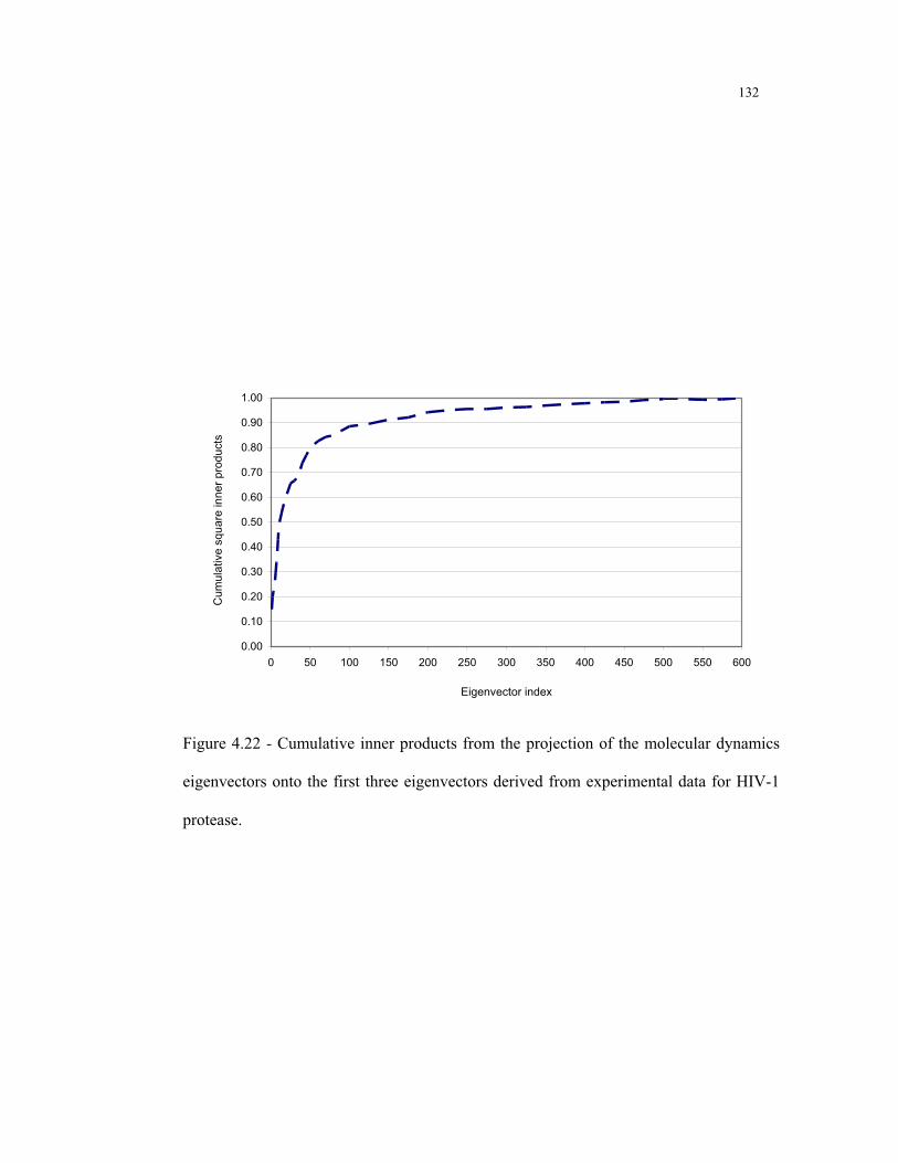
132

0.00

0.10

0.20

0.30

0.40

0.50

0.60

0.70

0.80

0.90

1.00

0 50 100 150 200 250 300 350 400 450 500 550 600

Eigenvector index

Cum

ula

tive

sq

ua

re in

ne

r p

rod

uct

s

Figure 4.22 - Cumulative inner products from the projection of the molecular dynamics

eigenvectors onto the first three eigenvectors derived from experimental data for HIV-1

protease.

133

Finally, we compared how the modes derived from molecular dynamics data

represented the original molecular dynamics data from which they were derived versus

the experimentally determined structures. This evaluation was carried out by comparing

how much the right singular vectors deviated from a normal distribution. If the modes

are a good representation for the data the most significant right singular vectors should

have a large deviation from a normal distribution whereas the least significant should

be normally distributed with a very small deviation from the mean. The right singular

vectors representative of the molecular dynamics data were calculated using the PCA

method as described previously and the right singular vectors for the experimental data

were determined by calculating the projection of the coordinate vectors of 135

experimentally determined structures on the left singular vectors from the molecular

dynamics backbone PCA. The metric used for comparison was the average deviation

from the mean. The results for the first 1000 modes are shown in Figure 4.23. The plots

show that the average deviation from the mean for the main modes is much larger for

the molecular dynamics data than for the experimental data. For the first mode this

value is 20.51 for the molecular dynamics data versus 3.15 for the experimental data.

The plot for the experimental data shows a decay for the average deviation which

would not happen for a random basis, indicating that there is relevant information for

HIV-1 protease motion that can be extracted from molecular dynamics data. A more

detailed view of these results can be obtained from right singular vector histograms.

Figure 4.24 show histograms for the 1st, 2

nd, 3

rd, and 1000

th right singular vector for the

molecular dynamics data and the experimental data. It is clear from these plots that the

134

modes are a good representation for the molecular dynamics data but not ideal for the

experimental data. The molecular dynamics data shows a much larger deviation from

the mean. In conclusion, the results of this section show that modes of motion derived

from molecular dynamics represent a valid basis to represent flexibility as observed

from experimental structures. However, there is still a significant amount of room for

improvement in the quality of modes. Improvement could result from increased

accuracy in the computational simulation of biological systems.

135

Figure 4.23 - Average deviation from the mean for the right singular vectors of the experimental and MD data.

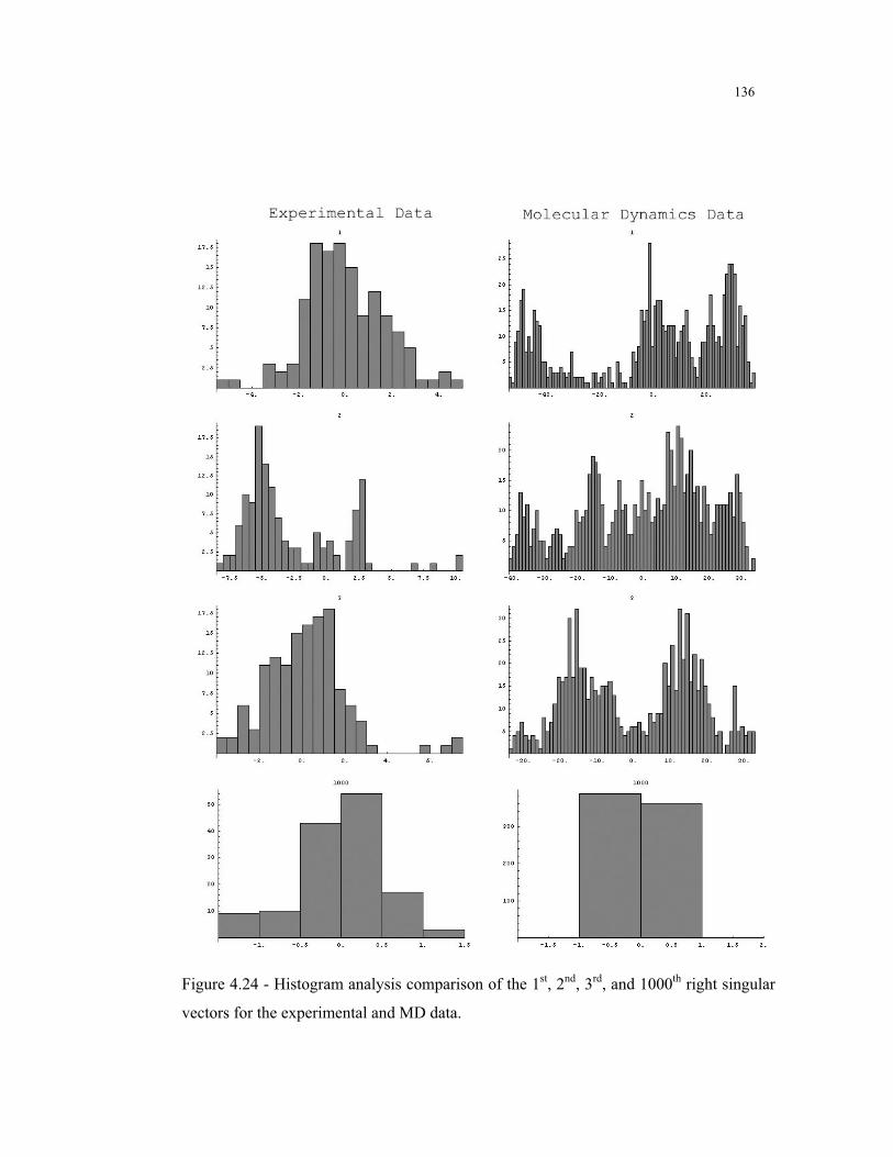
136

Figure 4.24 - Histogram analysis comparison of the 1st, 2

nd, 3

rd, and 1000

th right singular

vectors for the experimental and MD data.

137

4.5. Summary

In this chapter we show how to use the Principal Component Analysis (PCA)

method, a dimensionality reduction technique, to transform the original high-

dimensional representation of protein motion into a lower dimensional representation

that captures the dominant modes of motions of proteins. The method was applied to

HIV-1 protease, aldose reductase, and maltose binding protein. The conformational

sampling data used for the PCA calculation was obtained using molecular dynamics

techniques. For the case of HIV-1 protease, PCA was also computed using data derived

exclusively from experimental methods and the results compared to the molecular

dynamics method. One of the advantages of PCA is that it can be carried out at

different levels of detail by selecting only a particular set of atoms for a protein. Here

we described and compared the results obtained for the PCA analyses of backbone,

binding site and all atoms in the protein. The results obtained for the main modes of

motion correlate well with experimental data available for these proteins.

138

Chapter 5.

Applications of Collective Modes of Motion to

Pharmaceutical Drug Design

5.1. Introduction

The use of collective modes of motion has been explored previously to include

protein flexibility information in structure based drug design (Kolossvary and Guida

1996; Kolossvary and Guida 1999; Zacharias and Sklenar 1999; Kolossvary and Keseru

2001). This previous work was based on collective modes of motion derived from

normal mode calculations. The use of normal modes offers some advantages but also a

number of important limitations. The main advantage of using a normal modes based

method is speed in computing the collective modes of motion. Whereas the PCA

approach requires as input conformations obtained from a molecular simulation, which

can take several days to obtain, the normal modes approach only requires the

computation of the eigendecomposition of the Hessian. The Hessian is the matrix of

second derivatives of the potential energy with respect to the mass weighted molecular

coordinates. However, the normal modes approach assumes that the system moves

about an energy minimum and that the motion is harmonic. This is clearly not the case

for induced fit changes occurring at room temperature. In these conditions, the protein

will likely go through several conformational substates as it transitions from the bound

to the unbound conformation. As a result, the computation of modes from PCA (also

139

called quasi-harmonic analysis) is in our view a better approximation to include

collective modes of motion information in modeling induced fit processes.

In this chapter we discuss several approaches to include collective modes of

motion information in structure based drug design. In Sections 5.2 and 5.3 we discuss

indirect methods in which the SVD information is used to generate a set of

conformational samples that represent the flexibility of the protein. The individual

structures obtained using this method can later be used in current docking programs that

take as input the rigid three dimensional shape of the receptor. In Section 5.4 we

investigate the possibility of using the collective degrees of freedom directly to search

for alternative protein conformations.

5.2. Generating Docking Targets Using Collective Modes of Motion for

Conformational Sampling

One possible method of applying the information derived from the calculation

of collective modes of motion to model the flexibility of the protein is to use these to

efficiently generate a discrete set of conformations that represents alternative protein

conformations. The individual protein conformations can then be used with traditional

rigid-protein / flexible-ligand docking software without modifications to the original

programs. Protein conformational sampling using collective modes of motion is more

efficient because it is done along the degrees of freedom that are responsible for most

of the conformational variance observed during a computational simulation (or

alternatively in large amount of experimental data). The use of collective modes of

140

motion has been described before as a method to speed up conformational sampling

using molecular dynamics (Amadei, Linssen et al. 1996; de Groot, Amadei et al. 1996;

de Groot, Amadei et al. 1996). In this previous application, the modes of motion were

used as additional constraint forces in the simulation.

A simple method of generating a discrete conformational sampling is to use a

reference structure (i.e. experimental structure) and modify it in the direction of a

collective mode of motion. This type of perturbation is illustrated in Figures 4.4 to 4.7.

More than one direction can be used for the perturbation and more than one structure

can be generated along the direction of perturbation. In Figure 5.1 we show an example

in which we generate seven conformations along the first mode of motion and five

along the second mode of motion. The modes of motion can also be combined by

adding or subtracting the corresponding eigenvectors to generate structures along

directions diagonal to the original main motions. Although naïve, a grid based sampling

can be very easily generated and used for docking. One drawback of using this method

is that the structures generated along the modes of motion will display a large increase

in internal energy due to the deviations from ideal bond and angle geometry.

Nevertheless, this problem can be easily solved using a short conjugate gradient

minimization procedure. Our own experiments (results not shown) indicate that a short

conjugate gradient minimization protocol that takes less than ten seconds to complete

on a current desktop PC is enough to correct the deviation from ideal geometry and

restore the internal energy to initial values.

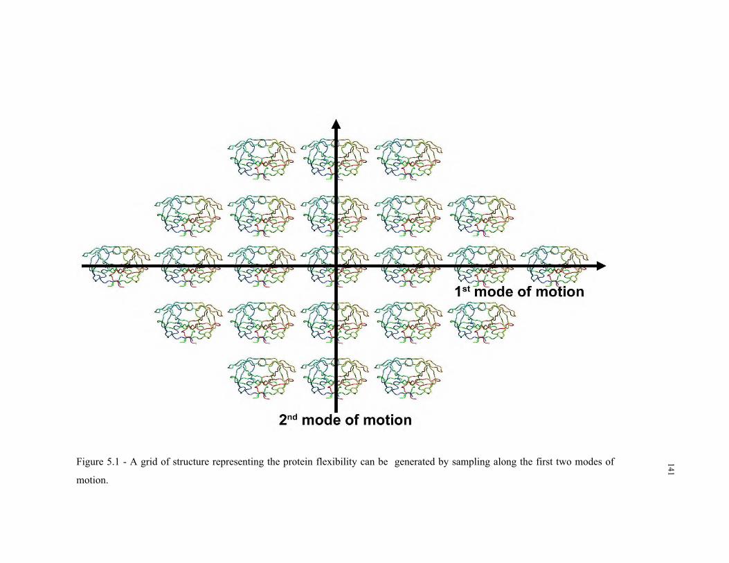
141

Figure 5.1 - A grid of structure representing the protein flexibility can be generated by sampling along the first two modes of

motion.

142

The main problem of using a discrete grid sampling to represent the flexibility

of the protein is that the size of the set will grow exponentially with the number of

degrees of freedom used to generate it. Fortunately, there are several factors that limit

the severity of this problem. The first factor is that it is not necessary to generate a large

number of structures along each mode. Our studies described in Chapter 2 indicate that

good docking results can be obtained using current rigid-protein / flexible-ligand

docking programs even when there is a non-negligible error (0.6Å – 1.2Å RMSD) in

the receptor model relative to the actual experimental structure of the docked receptor.

As a result, it is possible to generate a very low sampling along the main modes of

motion and rely on the error tolerance of the docking programs to compensate for

intermediate conformations that are skipped due to coarseness of the sampling. In

addition, it is possible to also modify the docking programs to accommodate for

additional accuracy errors relative to the docked conformation (Wojciechowski and

Skolnick 2002). A second factor that facilitates the use of the grid method is that,

although the problem is larger in size, it can be classified as an embarrassingly parallel

problem. This class of problems can be solved in a cost effective way by the use of

clusters of commodity type computers, such as common PC desktops.

The structures generated using a grid based approach can be used for

applications other than structure-based drug design in which the objective is to dock a

small molecule to a large macromolecule. Another potential application of this method

is to perform the docking of two macromolecules that undergo some level of

conformational change when they interact. Instead of modeling flexibility explicitly

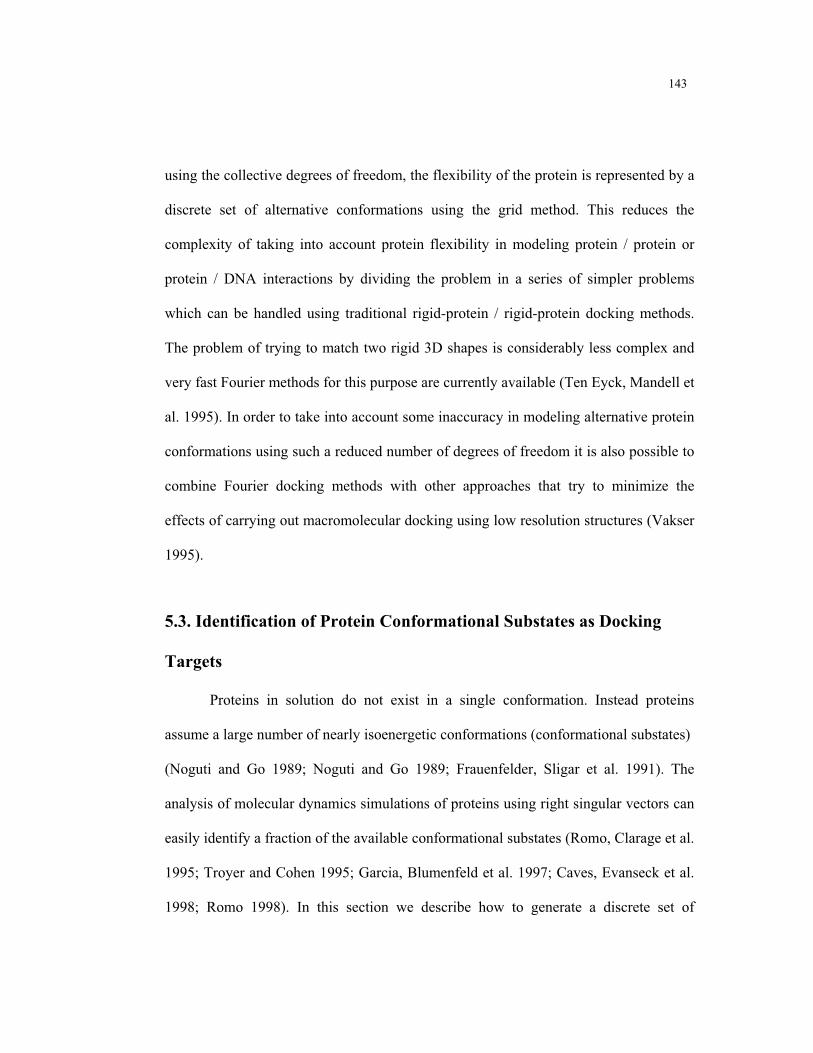
143

using the collective degrees of freedom, the flexibility of the protein is represented by a

discrete set of alternative conformations using the grid method. This reduces the

complexity of taking into account protein flexibility in modeling protein / protein or

protein / DNA interactions by dividing the problem in a series of simpler problems

which can be handled using traditional rigid-protein / rigid-protein docking methods.

The problem of trying to match two rigid 3D shapes is considerably less complex and

very fast Fourier methods for this purpose are currently available (Ten Eyck, Mandell et

al. 1995). In order to take into account some inaccuracy in modeling alternative protein

conformations using such a reduced number of degrees of freedom it is also possible to

combine Fourier docking methods with other approaches that try to minimize the

effects of carrying out macromolecular docking using low resolution structures (Vakser

1995).

5.3. Identification of Protein Conformational Substates as Docking

Targets

Proteins in solution do not exist in a single conformation. Instead proteins

assume a large number of nearly isoenergetic conformations (conformational substates)

(Noguti and Go 1989; Noguti and Go 1989; Frauenfelder, Sligar et al. 1991). The

analysis of molecular dynamics simulations of proteins using right singular vectors can

easily identify a fraction of the available conformational substates (Romo, Clarage et al.

1995; Troyer and Cohen 1995; Garcia, Blumenfeld et al. 1997; Caves, Evanseck et al.

1998; Romo 1998). In this section we describe how to generate a discrete set of

144

conformations that best represents the conformational substates observed for a

molecular dynamics simulation. The set of structures can then be used for rigid-protein

/ flexible-ligand docking.

The right singular vector results for the binding site of HIV-1 protease, aldose

reductase and maltose binding protein discussed in Section 4.4.3 clearly show that these

proteins do not move at a fixed velocity in conformational space. Instead they hop

between stable conformational substates. Using the plots in Figures 4.17 to 4.19 it is

possible to identify at what times during the simulation the protein resides in a

particular conformational substate. In order to select a representative structure from

each of the conformational substates we calculated pairwise root mean square distances

between individual structures within the same conformational substate. The distance

metric used was not the Cartesian RMSD. Instead distances were calculated in the

space defined by the first three modes of motion (Figures 4.17 to 4.19) and the structure

with the lowest mean root mean square distance to the other members of the substate

was selected to be its representative. It would also be possible to use the Cartesian

RMSD as a distance metric to select the representative structure. However such

computation would be significantly more expensive because it would require the

computation of a distance in a space with 750 dimensions versus 3.

Results for the identification of conformational substate representatives for the

three model proteins analyzed in Chapter 4 are shown in Figure 5.2 to 5.4. Figure 5.2

shows the results for HIV-1 protease. The three representative structures corresponding

to conformational substates A, B and C are colored using red, yellow and green,

145

respectively. The conformations correspond to largely different binding site shapes. The

red conformation displays the smallest binding site and the green conformation the

largest. The large differences in binding site volume are consistent with experimentally

determined structures which show variations in volume larger than 100%. In Figure

5.2-b) we show a magnified view of the binding site residues show in a). The increase

in binding site volume is a result of rotations of some of the residue sidechains but is

mostly due to a coordinated motion at the backbone level. The two conformational

representatives for aldose reductase are shown in Figure 5.3. In this case the alternative

conformations represent more localized changes. In Figure 5.3-b) the white arrow

indicates residue LEU 300. Changes in this residue and its vicinity are responsible for

most of the opening of the extra cavity that distinguishes the bound conformations with

sorbinil and tolrestat (for more information see Appendix A.2). This observation

constitutes a positive result for the applicability of the right singular vectors method.

Starting from the conformation for one of the ligands it was possible to computationally

generate a conformation which could be used successfully to screen a different class of

ligands. Finally, in Figure 5.4 we show three different conformational representatives

for maltose binding protein. In this case the conformational changes are smaller than in

the other two cases but may help understand how maltose binding protein changes its

conformation when binding different maltodextrins and cyclodextrins.

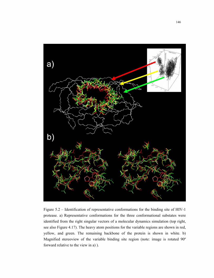
146

Figure 5.2 – Identification of representative conformations for the binding site of HIV-1

protease. a) Representative conformations for the three conformational substates were

identified from the right singular vectors of a molecular dynamics simulation (top right,

see also Figure 4.17). The heavy atom positions for the variable regions are shown in red,

yellow, and green. The remaining backbone of the protein is shown in white. b)

Magnified stereoview of the variable binding site region (note: image is rotated 90º

forward relative to the view in a) ).

147

Figure 5.3 – Identification of representative conformations for the binding site of aldose

reductase. a) Two conformations were identified using the right singular vectors (top

right, see also Figure 4.18). b) Magnified stereoview of the variable binding site region.

148

Figure 5.4 - Identification of representative conformations for the binding site of maltose

binding protein. a) Two conformations were identified using the right singular vectors

(top right, see also Figure 4.18). b) Magnified stereoview of the variable binding site

region.

149

The method described in this section to generate a discrete conformational

sampling for the flexibility of the protein has advantages and disadvantages relative to

the grid method described in the previous section. The main advantage is that the

number of structures generated is much smaller. Furthermore, the structures generated

are of better quality in the sense that they correspond to low energy regions of the

potential energy landscape. However, the main disadvantage is that even long

molecular dynamics simulations only cover a small fraction of the conformational

landscape (Clarage, Romo et al. 1995). As such, it is likely that the grid method

provides a better coverage of the available conformational space.

An alternative application for the identification of stable conformational

substates using the information from the right singular vectors is to improve the design

of dynamic pharmacophore models (Carlson, Masukawa et al. 1999; Carlson,

Masukawa et al. 2000). The pharmacophore is a three dimensional arrangement of

molecular features that is present in all (or most) of the active conformations of a set of

drug molecules that interact with a given receptor. Hence, the pharmacophore can be

viewed as a geometric invariant of the active conformations of the considered

molecules. The dynamic pharmacophore model extends this concept by using as a

receptor model several conformations obtained using a molecular dynamics trajectory.

The dynamic pharmacophore model is described by binding regions that are conserved

over many protein conformations. In their work Carlson et al selected conformations

from the molecular dynamics trajectory at fixed time intervals. Given the “beads-on-a-

string” nature of protein dynamics this is probably not the most effective choice. Fixed

150

time intervals are likely to select more than one structure from each conformational

substate (leading to wasted effort) or miss a structure from a particular conformational

substate (leading to lack of coverage of the conformational space). A better alternative

is to use the right singular vectors to identify protein conformational substates and use

representative structures in the pharmacophore calculation.

5.4. Approximating Molecular Conformations Using Low Dimensional

Representations for Protein Flexibility

A third method of using the information derived from the calculation of

collective modes of motion to model the flexibility of the protein is to use these degrees

of freedom directly in the conformational search for the docked ligand. Such a method

could be easily included in most current rigid-protein / flexible-ligand docking

programs by adding degrees of freedom of the protein to the existing search space. For

example, to add protein flexibility capabilities to Autodock (Morris, Goodsell et al.

1998) we would only need to extend the information in the chromosome to include the

new degrees of freedom representing the protein (note: Autodock uses a genetic

algorithm to search the conformational space of the ligand to find the docked

conformation (for more details see Appendix C) ). However, if we are to perform the

conformational search directly by dealing with the degrees of freedom of the protein in

the same manner as the degrees of freedom of the ligand then two important questions

arise: “How many degrees of freedom of the protein need to be included in the

151

conformational search?” and “What level of approximation can we obtain using the

reduced basis of representation?”. In this section we will address these two questions.

In order to answer the two questions we decided to investigate if using the main

modes of motion defined by the principal components and an experimental structure

bound to a particular ligand, we could approximate the structure of HIV-1 protease

bound to a different ligand. For this experiment we were only concerned with variations

in the shape of the binding site and used only the PCA results described in Chapter 4

for this part of the protein. A total of 250 atoms constitute the binding site for HIV-1

protease, which results in an initial search space of 750 dimensions. As the initial

reference conformation we chose the same structure we used for the molecular

dynamics simulation and as a target structure we used a complex with a large non-

peptide inhibitor (Rutenber, Fauman et al. 1993) (PBD access code 1AID). The binding

site conformations as well as the inhibitors bound to these are considerably different as

shown in Figure A.2. The root mean square deviation (RMSD) between the two

proteins is 1.843 Å if we take into account only the atoms that constitute the binding

site.

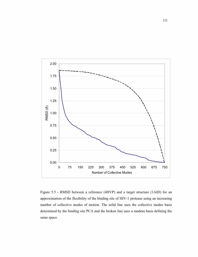
152

0.00

0.25

0.50

0.75

1.00

1.25

1.50

1.75

2.00

0 75 150 225 300 375 450 525 600 675 750

Number of Collective Modes

RM

SD

(Å

)

Figure 5.5 - RMSD between a reference (4HVP) and a target structure (1AID) for an

approximation of the flexibility of the binding site of HIV-1 protease using an increasing

number of collective modes of motion. The solid line uses the collective modes basis

determined by the binding site PCA and the broken line uses a random basis defining the

same space.

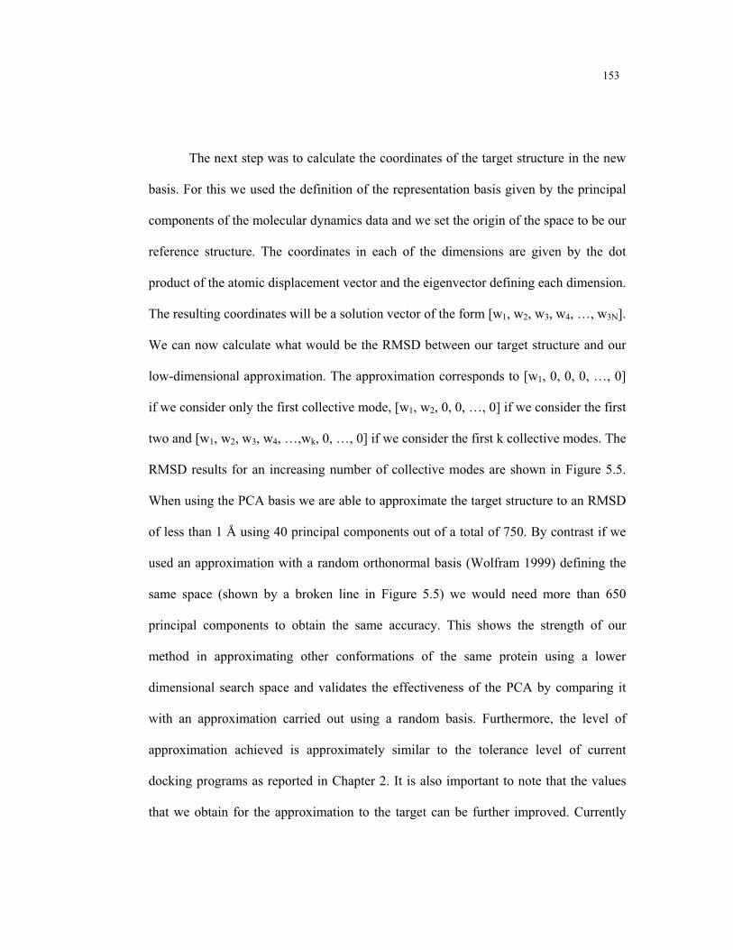
153

The next step was to calculate the coordinates of the target structure in the new

basis. For this we used the definition of the representation basis given by the principal

components of the molecular dynamics data and we set the origin of the space to be our

reference structure. The coordinates in each of the dimensions are given by the dot

product of the atomic displacement vector and the eigenvector defining each dimension.

The resulting coordinates will be a solution vector of the form [w1, w2, w3, w4, …, w3N].

We can now calculate what would be the RMSD between our target structure and our

low-dimensional approximation. The approximation corresponds to [w1, 0, 0, 0, …, 0]

if we consider only the first collective mode, [w1, w2, 0, 0, …, 0] if we consider the first

two and [w1, w2, w3, w4, …,wk, 0, …, 0] if we consider the first k collective modes. The

RMSD results for an increasing number of collective modes are shown in Figure 5.5.

When using the PCA basis we are able to approximate the target structure to an RMSD

of less than 1 Å using 40 principal components out of a total of 750. By contrast if we

used an approximation with a random orthonormal basis (Wolfram 1999) defining the

same space (shown by a broken line in Figure 5.5) we would need more than 650

principal components to obtain the same accuracy. This shows the strength of our

method in approximating other conformations of the same protein using a lower

dimensional search space and validates the effectiveness of the PCA by comparing it

with an approximation carried out using a random basis. Furthermore, the level of

approximation achieved is approximately similar to the tolerance level of current

docking programs as reported in Chapter 2. It is also important to note that the values

that we obtain for the approximation to the target can be further improved. Currently

154

we are using the projection of the target structure on the new basis to estimate a set of

coordinates in the reduced space that approximate the target structure. However, the

optimal approach is to search the low-dimensional space directly to look for the best

match. In this way we can search for alternative coordinate values along the most

significant principal components that compensate for the approximation being

introduced by the dimensional truncation of the representation basis. We are currently

developing search techniques for the purpose of finding these solutions in the reduced

space.

Despite the promising results of the previous experiment it is important to note

that during the course of our investigation we found two factors which are critical in

order to obtain good results using the reduced basis representation for protein

flexibility. The first factor is that the PCA should be restricted to the region of interest.

For the case of docking applications this would be the binding site region. In Figure 5.6

we show the results of an approximation experiment equal to the one described in the

previous paragraph but using the collective modes of motion determined for the all-

atoms PCA instead of the binding site PCA. From the comparison of Figures 5.5 and

5.6 we can conclude that although the all-basis atoms also provides a better description

of protein flexibility than a random basis, the approximation is significantly worse that

for the binding site case. The reason for this is that the all-atoms modes of motion have

to account for several changes in conformation that are not relevant at the binding site

level.

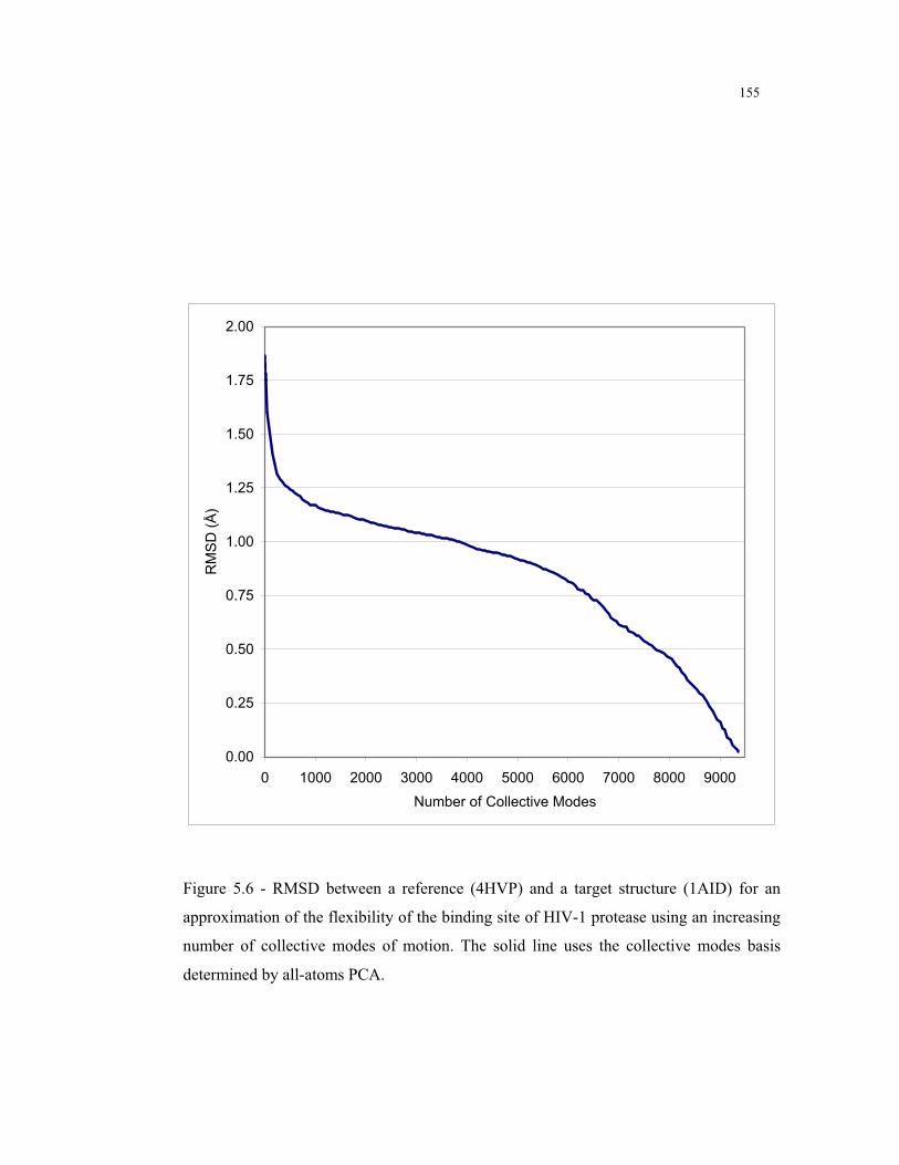
155

0.00

0.25

0.50

0.75

1.00

1.25

1.50

1.75

2.00

0 1000 2000 3000 4000 5000 6000 7000 8000 9000

Number of Collective Modes

RM

SD

(Å

)

Figure 5.6 - RMSD between a reference (4HVP) and a target structure (1AID) for an

approximation of the flexibility of the binding site of HIV-1 protease using an increasing

number of collective modes of motion. The solid line uses the collective modes basis

determined by all-atoms PCA.

156

0.00

0.25

0.50

0.75

1.00

1.25

1.50

1.75

2.00

0 75 150 225 300 375 450 525 600 675 750

Number of Collective Modes

RM

SD

(Å

)

Figure 5.7 - RMSD between a reference (4HVP) and a target structure (9HVP) for an

approximation of the flexibility of the binding site of HIV-1 protease using an increasing

number of collective modes of motion. The solid line uses the collective modes basis

determined by binding site PCA.

157

The second pitfall we discovered when testing the modes of motion derived

from PCA is that they are useful only when modeling conformational rearrangements

larger than 1.0Å to 1.2Å. In Figure 5.7 we show an experiment equal to the one

described for Figure 5.5 but instead of approximating the binding site structure of 1AID

we used the structure with PDB code 9HVP. The initial difference at the level of the

binding site for these two structures is 0.9Å RMSD. As can be observed from Figure

5.7 the inclusion of first main modes of motion does not lead to a sharp increase in the

level of approximation as was observed in Figures 5.5 and 5.6. On the contrary, the

approximation increases almost linearly with the number of degrees of freedom used

for modeling. The linear phase is also present in Figure 5.5 starting at approximately

0.9Å RMSD as well as in over 100 other conformations with different initial levels of

approximation for which we tested this procedure (results not shown). The main

conclusion for all the experiments is that approximately 30-50 main modes of motion

are sufficient to generate an approximation at the level of 0.9Å RMSD but beyond this

threshold the main modes of motion provide very little useful information. The

justification for this result lies in a fundamental limitation of the PCA method. The

PCA method relies on the accurate computation of motion correlation between pairs of

atoms. If there is a large amount of uncorrelated motion present, such as random

thermal motion, it will mask any smaller amplitude correlated motions present in the

system and in practice render modes of motion corresponding to very small deviations

useless. Fortunately, in light of the results reported in Chapter 2 the 1.0Å approximation

threshold is not a major problem for docking applications.

158

0.00

0.25

0.50

0.75

1.00

1.25

1.50

1.75

2.00

0 50 100 150 200 250 300 350 400 450

Number of Collective Modes

RM

SD

(Å

)

Figure 5.8 - RMSD between a reference (1AH4) and a target structure (1AH3) for an

approximation of the flexibility of the binding site of aldose reductase using an increasing

number of collective modes of motion. The solid line uses the collective modes basis

determined by binding site PCA.

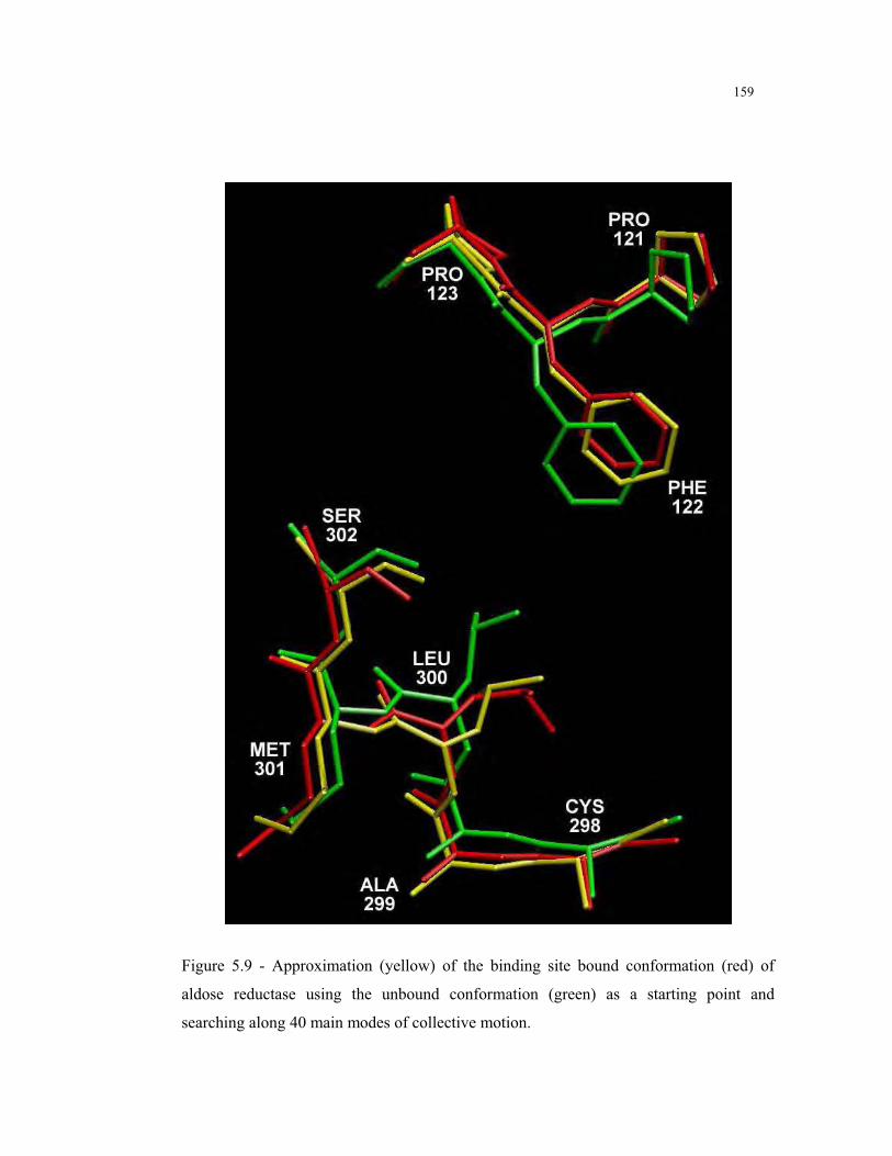
159

Figure 5.9 - Approximation (yellow) of the binding site bound conformation (red) of

aldose reductase using the unbound conformation (green) as a starting point and

searching along 40 main modes of collective motion.

160

In order to test the ability to use PCA modes of motion as degrees of freedom

for modeling proteins other than HIV-1 protease we also applied the testing

methodology described in this section to aldose reductase. For this we calculated an

approximation of the form [w1, w2, …, w40, 0, …, 0] as we did for HIV-1 protease

using the unbound form as the reference structure (no pocket present) and the bound

structure to tolrestat as our target (pocket is present). The RMSD evolution for the

binding site residues is shown in Figure 5.8. Figure 5.9 shows the approximation

(yellow) of the bound conformation (red) using the unbound conformation (green) as a

starting point and searching along 40 main modes of collective motion. The initial

difference between the bound and unbound forms is 1.93Å RMSD. Using a 40 degrees

of freedom approximation we can reduce this value to 1.03Å. From the figure it is clear

that we can obtain a good approximation on the residues that form the top of the

specificity pocket with our approximate structure matching almost exactly the

experimental structure for the bound form. It is important to note that the approximation

is able to capture not only the movement of aminoacid sidechains, such as the rotation

of the aromatic ring in PHE 122, but also global displacements caused by a movement

at the backbone level, such as shown for the backbone of residues 121 to 123. This

contrasts with complexity reduction methods that consider the important flexibility of

the protein as being represented only by movements of sidechains and that are unable to

represent induced fit conformational changes caused by backbone movements. The

bottom part of the specificity pocket does not show a match of similar quality but still

shows a trend in the right direction. A good example of this is the change in

161

conformation of LEU 300. In fact the approximated structure already displays the

specificity pocket and is large enough to accommodate ligands such as tolrestat or

zopolrestat.

5.5. Summary

In this chapter we explore different methods of including the information

derived from the dimensional reduction of molecular dynamics trajectories to model

protein flexibility in the context of structure-based drug design. The information can be

used indirectly to generate a discrete set of conformational samples that represent the

flexibility of the protein. The sampled conformations can later be used as target

receptors using traditional rigid-protein / flexible-ligand programs. Two methods are

described to generate the conformational sampling: one is based on grid sampling along

the main modes of motion, and the other is based on the identification of a

representative structure of conformational substates using right singular vectors.

Alternatively, the modes of motion can be used directly in conjunction with the degrees

of freedom in the ligand to search for a flexible-protein / flexible-ligand bound

conformation. Although there is inevitably some loss in accuracy, we show that we can

obtain conformations that have been observed in laboratory experiments, starting from

different initial conformations and working in a drastically reduced search space.

162

Chapter 6.

Conclusions

In this work we showed how to obtain a reduced basis representation of protein

flexibility. Proteins typically have a few hundreds to a few thousands of degrees of

freedom. Starting with data obtained from laboratory experiments and/or molecular

dynamics simulations, we demonstrate that we can compute a new set of degrees of

freedom that are combinations of the original ones and that can be ranked according to

significance. Depending on the level of accuracy desired, the k most significant of these

new degrees of freedom can be used to model the flexibility of the system. We have

observed, in multiple occasions, that the reduced basis representation retains critical

information about the directions of preferred motion of the protein. It can thus be used

to compute conformational rearrangements of the protein that can further be studied for

interaction with novel ligands or other proteins. Our work contributes to the better

understanding of how changes in the conformation of a protein affect its ability to bind

other molecules and hence its function. We envision that protein databases, such as the

Protein Data Bank, would be annotated in the future with principal modes of motion for

proteins allowing rapid and detailed analysis of biomolecular interactions. This

annotation would allow researchers not only to analyze the static structure of a protein

but also its motions and relations between structure, motion and function. The process

of determining collective modes of motion could be automated using the methods

described in the present work and the information would complement other structural

163

databases such as the Database of Macromolecular Movements (Gerstein and Krebs

1998).

In this work we used PCA as our dimensionality reduction technique. The

results obtained are biologically meaningful. Clearly, it is worth investigating the

application of non-linear dimensionality reduction techniques to the same problem. For

example local PCA (Kambhatla and Leen 1997), locally linear embedding (Roweis and

Saul 2000), and multi-layer auto-associative neural networks (Kramer 1991) might be

able to provide us with the same kind of information as PCA while using an even

further reduced number of degrees of freedom. The application of these dimensionality

reduction methods to protein structural data is only practical for modeling if we are able

to obtain an inverse mapping from the lower to the higher dimensional space. This

mapping can in principle be obtained using machine learning techniques such as neural

networks. Carrying out this step efficiently is very difficult and constitutes an open

research question. Preliminary work in our group indicates that some of the advantages

obtained by performing a non-linear dimensional reduction are outweighed by an

increased computational cost and a loss in accuracy due to the approximated inverse

mapping. Nevertheless, the advantage of reduced complexity in the representation of

molecular motion may justify the increased computational cost of the non-linear

dimensionality reduction depending on the application.

All our work was done using the Cartesian coordinates of atoms in the protein.

An interesting idea is to perform the dimension reduction in the dihedral and the bond

angle space of the system. The advantage of this approach is that the initial

164

dimensionality of the problem is reduced because given certain constraints fewer

parameters are necessary to uniquely define a protein structure. The first constraint is

that bond lengths are fixed. At a second level of approximation, bond angles between

three consecutively bonded atoms can also be considered fixed. As such, it is possible

to represent a molecular conformation using only the set of dihedral angles

corresponding to torsions around single bonds. The dimensionality of this space is in

practice approximately almost an order of magnitude smaller than the Cartesian

representation. Initial experiments showed that a dihedral angle-based analysis of

conformational data is very sensitive to noise and prone to error. We are currently

investigating this problem and improving the general methodology in order to apply the

methods described in this work to a dihedral angle representation. Last but not least, we

investigate how to effectively explore conformational flexibility of a protein in the

reduced basis representation to make approximate but fairly accurate predictions for

protein-protein and protein-ligand interactions. This work could be used to predict

complex effects such as the induced fit effect during ligand binding in a drug design

study in a computationally efficient manner.

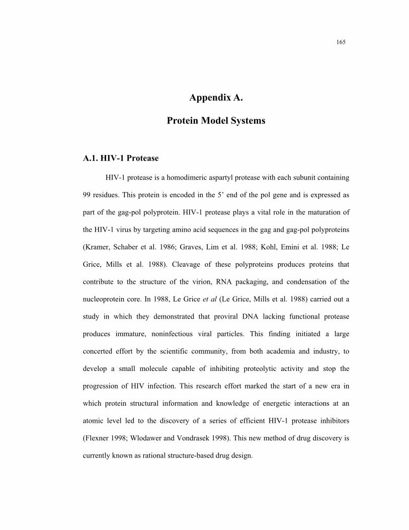
165

Appendix A.

Protein Model Systems

A.1. HIV-1 Protease

HIV-1 protease is a homodimeric aspartyl protease with each subunit containing

99 residues. This protein is encoded in the 5’ end of the pol gene and is expressed as

part of the gag-pol polyprotein. HIV-1 protease plays a vital role in the maturation of

the HIV-1 virus by targeting amino acid sequences in the gag and gag-pol polyproteins

(Kramer, Schaber et al. 1986; Graves, Lim et al. 1988; Kohl, Emini et al. 1988; Le

Grice, Mills et al. 1988). Cleavage of these polyproteins produces proteins that

contribute to the structure of the virion, RNA packaging, and condensation of the

nucleoprotein core. In 1988, Le Grice et al (Le Grice, Mills et al. 1988) carried out a

study in which they demonstrated that proviral DNA lacking functional protease

produces immature, noninfectious viral particles. This finding initiated a large

concerted effort by the scientific community, from both academia and industry, to

develop a small molecule capable of inhibiting proteolytic activity and stop the

progression of HIV infection. This research effort marked the start of a new era in

which protein structural information and knowledge of energetic interactions at an

atomic level led to the discovery of a series of efficient HIV-1 protease inhibitors

(Flexner 1998; Wlodawer and Vondrasek 1998). This new method of drug discovery is

currently known as rational structure-based drug design.

166

Figure A.1 - 3D structure of HIV-1 protease homodimer complexed with an inhibitor.

On the a) top view and b) side view the -hairpin flaps wrapping around the ligand are

shown. c) in a space filling view the tight fit of the ligand in the binding site is shown

indicating the need for a protein motion to allow for ligand entry and exit.

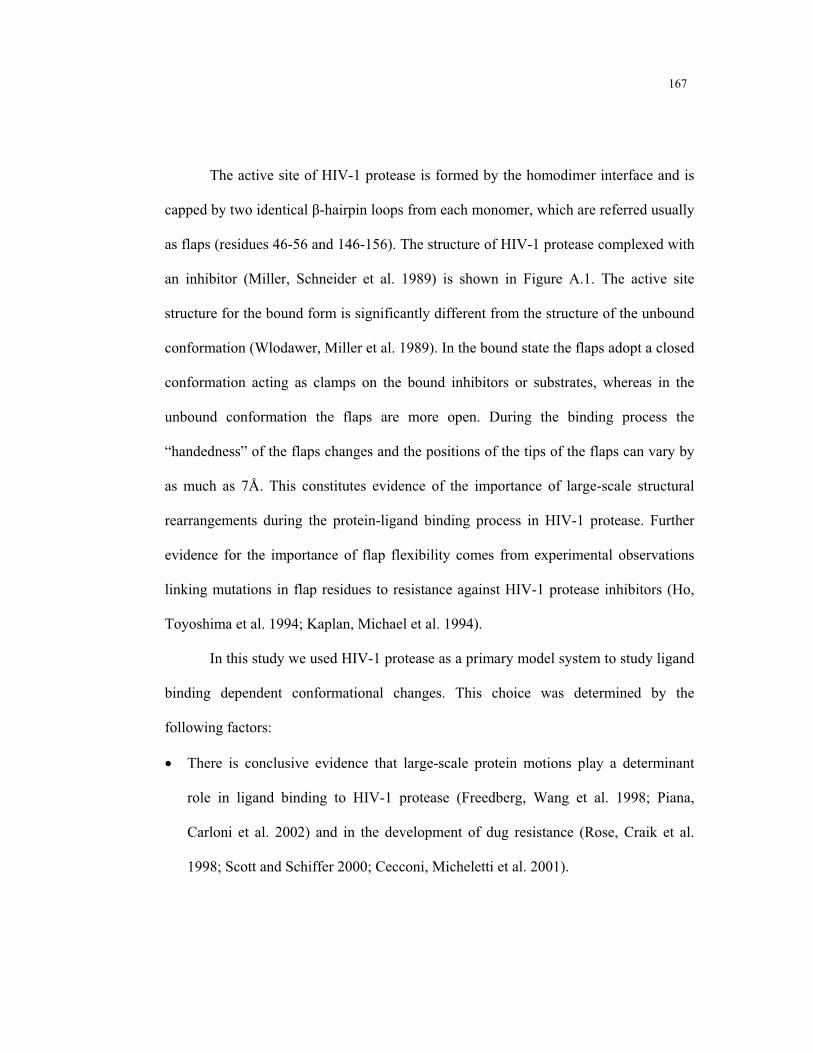
167

The active site of HIV-1 protease is formed by the homodimer interface and is

capped by two identical -hairpin loops from each monomer, which are referred usually

as flaps (residues 46-56 and 146-156). The structure of HIV-1 protease complexed with

an inhibitor (Miller, Schneider et al. 1989) is shown in Figure A.1. The active site

structure for the bound form is significantly different from the structure of the unbound

conformation (Wlodawer, Miller et al. 1989). In the bound state the flaps adopt a closed

conformation acting as clamps on the bound inhibitors or substrates, whereas in the

unbound conformation the flaps are more open. During the binding process the

“handedness” of the flaps changes and the positions of the tips of the flaps can vary by

as much as 7Å. This constitutes evidence of the importance of large-scale structural

rearrangements during the protein-ligand binding process in HIV-1 protease. Further

evidence for the importance of flap flexibility comes from experimental observations

linking mutations in flap residues to resistance against HIV-1 protease inhibitors (Ho,

Toyoshima et al. 1994; Kaplan, Michael et al. 1994).

In this study we used HIV-1 protease as a primary model system to study ligand

binding dependent conformational changes. This choice was determined by the

following factors:

There is conclusive evidence that large-scale protein motions play a determinant

role in ligand binding to HIV-1 protease (Freedberg, Wang et al. 1998; Piana,

Carloni et al. 2002) and in the development of dug resistance (Rose, Craik et al.

1998; Scott and Schiffer 2000; Cecconi, Micheletti et al. 2001).

168

HIV-1 protease as been extensively used as a model in computational studies. These

studies included flap opening dynamics, protein-ligand complex dynamic

flexibility, combined quantum/classical molecular dynamics studies, reaction path

free energy calculations (Collins, Burt et al. 1995; Liu, Muller-Plathe et al. 1996;

Luo, Kato et al. 1998; Rick, Erickson et al. 1998; Rick, Topol et al. 1998;

Ringhofer, Kallen et al. 1999; Piana and Carloni 2000).

There is extensive information on the mechanism and kinetics of HIV-1 protease

(Silva, Cachau et al. 1996; Flexner 1998; Todd and Freire 1999).

There are close to two hundred structures of HIV-1 protease bound to different

ligands available in the Protein Data Bank (Berman, Westbrook et al. 2000). This

variety serves as an excellent demonstration of protein plasticity in its optimal

adaptation to a flexible ligand (see Figure A.2). Furthermore, it allowed for

collective modes of motion to be calculated directly, based on the structural

variations observed experimentally.

Finding more efficient HIV-1 protease inhibitors is of extreme importance, since

currently available drugs require a combination therapy to avoid the development of

viral resistance and must be taken in very high dosages leading to serious side

effects (Flexner 1998; Molla, Granneman et al. 1998; Kaul, Cinti et al. 1999).

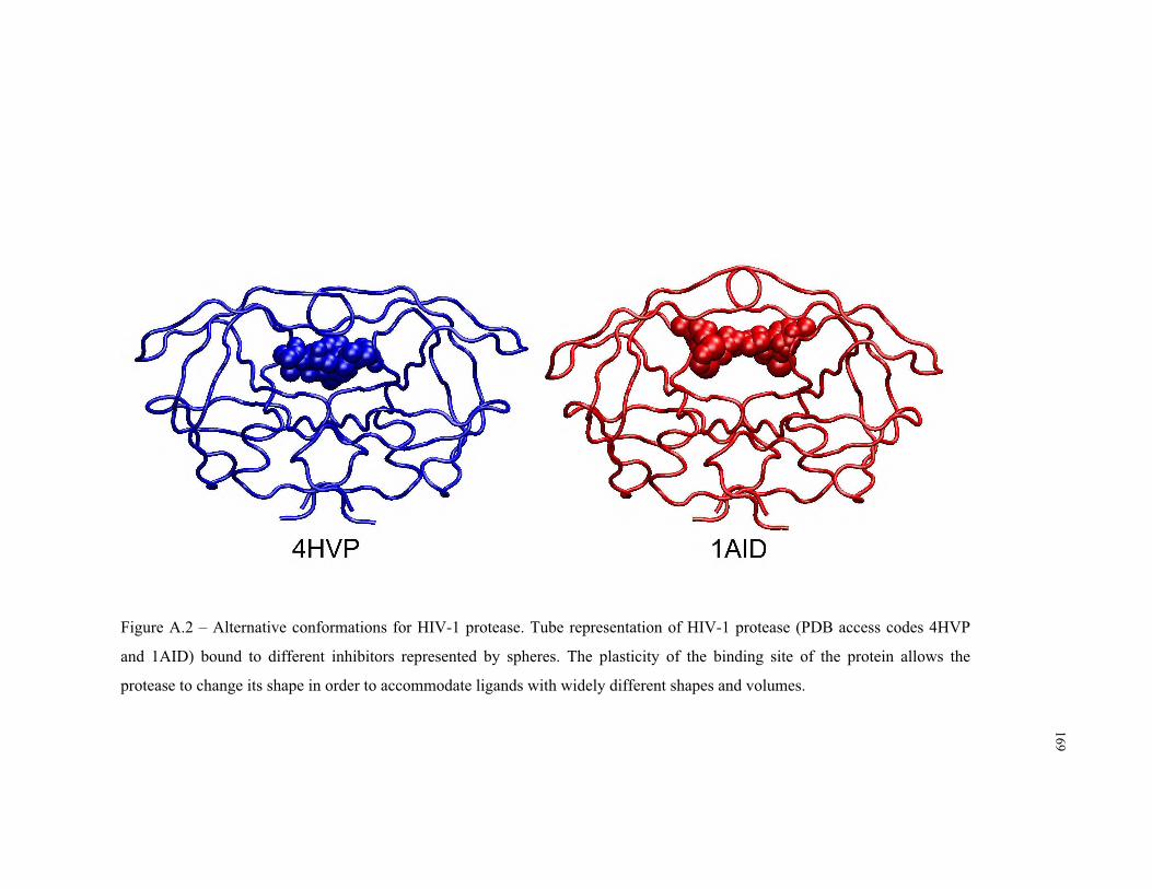
169

Figure A.2 – Alternative conformations for HIV-1 protease. Tube representation of HIV-1 protease (PDB access codes 4HVP

and 1AID) bound to different inhibitors represented by spheres. The plasticity of the binding site of the protein allows the

protease to change its shape in order to accommodate ligands with widely different shapes and volumes.

170

A.2. Aldose Reductase

Aldose reductase is a member of the aldo-keto reductase superfamily and is

responsible for the first step of the polyol metabolic pathway to catalyze the reduction

of glucose to sorbitol. This reaction uses nicotinamide adenine dinucleotide phosphate

(NADPH) as a cofactor. Sorbitol is subsequently transformed to fructose by sorbitol

dehydrogenase using a NAD+-dependent oxidation. Aldose reductase is of great

pharmacological interest due to its role in the development of complications associated

with diabetes mellitus (Oates and Mylari 1999). Namely, the development of

retinophaties, cataracts and glaucoma is believed to be due to the osmotic effect caused

by an increase in the concentration of sorbitol in the eye (Kinoshita and Nishimura

1988). Moreover, complications such as neuropathy and nephropathy are also caused

by the increase flux of glucose in the polyol pathway (Dunlop 2000). The development

of inhibitors for aldose reductase has been a goal in the pharmaceutical research field

for over 25 years. Some inhibitors, such as epalrestat, have shown positive results in the

treatment of diabetic complications. This drug is currently approved and marketed in

Japan for treatment of neuropathy associated with diabetes. Unfortunately, several

inhibitors such as tolrestat and sorbinil that showed some promise in laboratory and

clinical trials have been discarded due to problems associated with efficacy and safety

of these drugs. Efforts are still underway to find better inhibitors for aldose reductase

that display fewer side effects.

171

Figure A.3 – Superposition of the unbound (green) and bound (red) forms of aldose

reductase. The cofactor NADPH is shown using the orange sphere model. Unlike the

other protein models used in the present study, the conformational differences at the

backbone level are very small. However, the main changes occur in the binding site

region (indicated by B) and play a critical role in determining the binding to inhibitors of

different shapes.

172

Aldose reductase has a molecular weight of approximately 36 KDa. Analysis of

the crystal structure of human aldose reductase (Borhani, Harter et al. 1992; Wilson,

Bohren et al. 1992) shows that this protein belongs to the family of ( / )8 folding

proteins (see Figure A.3). The structure contains eight parallel -strands forming the

core of the barrel with each -strand alternating with an anti-parallel -helix. NADPH

binds at the carboxy-terminus of the enzyme in an extended conformation, making a

total of nineteen hydrogen bonds and three salt links with amino acid residues

composing the cofactor binding site.

One of the problems in developing new inhibitors for aldose reductase is that,

just like in the case of the other proteins in this study, this enzyme has the capacity to

adjust the shape of its binding site depending on the ligand it binds to. As such, a

simple small-molecule database screen for potential ligands will miss many potential

drug leads if it does not include the protein flexibility in the search process. Several

experimental structures of aldose reductase have been solved using X-ray

crystallography when bound to different ligands as well as in the unbound form (Figure

A.3). It was observed that with some inhibitors such as sorbinil (Urzhumtsev, Tete-

Favier et al. 1997), the structure is almost identical to the unbound form. For other

inhibitors, such as the tolrestat (Urzhumtsev, Tete-Favier et al. 1997) and zopolrestat

(Wilson, Tarle et al. 1993), there is a formation of a specificity pocket resulting in

significantly different binding site configurations. This conformational change is shown

in A.4 where we compare the shape of the binding site for the unbound form of the

enzyme to the bound form with tolrestat. In the unbound form shown on the left of A.4

173

there are two groups of aminoacids (represented by ball-and-stick models) that come

together to close the specificity pocket. In the presence of tolrestat (represented on the

right by a van der Waals sphere model) the aminoacids at the top and bottom of the

binding site are separated and open the specificity cavity. The movement is caused by

both side chain and small backbone rearrangements.

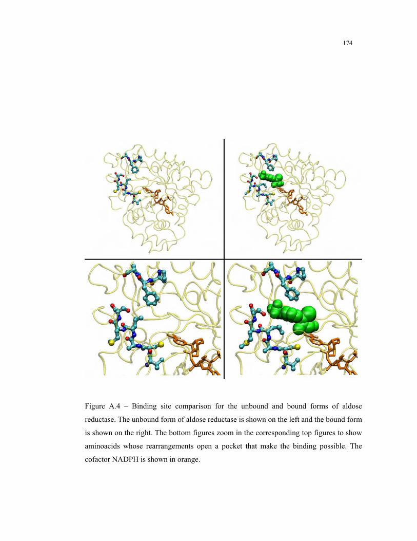
174

Figure A.4 – Binding site comparison for the unbound and bound forms of aldose

reductase. The unbound form of aldose reductase is shown on the left and the bound form

is shown on the right. The bottom figures zoom in the corresponding top figures to show

aminoacids whose rearrangements open a pocket that make the binding possible. The

cofactor NADPH is shown in orange.

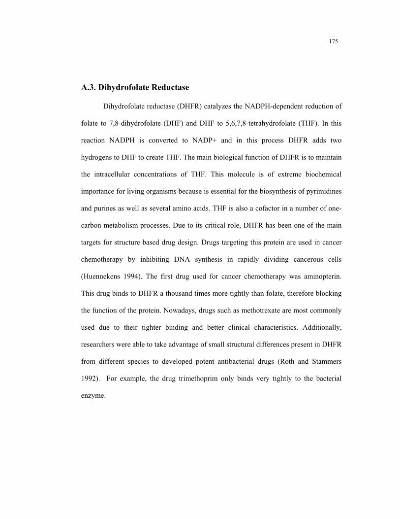
175

A.3. Dihydrofolate Reductase

Dihydrofolate reductase (DHFR) catalyzes the NADPH-dependent reduction of

folate to 7,8-dihydrofolate (DHF) and DHF to 5,6,7,8-tetrahydrofolate (THF). In this

reaction NADPH is converted to NADP+ and in this process DHFR adds two

hydrogens to DHF to create THF. The main biological function of DHFR is to maintain

the intracellular concentrations of THF. This molecule is of extreme biochemical

importance for living organisms because is essential for the biosynthesis of pyrimidines

and purines as well as several amino acids. THF is also a cofactor in a number of one-

carbon metabolism processes. Due to its critical role, DHFR has been one of the main

targets for structure based drug design. Drugs targeting this protein are used in cancer

chemotherapy by inhibiting DNA synthesis in rapidly dividing cancerous cells

(Huennekens 1994). The first drug used for cancer chemotherapy was aminopterin.

This drug binds to DHFR a thousand times more tightly than folate, therefore blocking

the function of the protein. Nowadays, drugs such as methotrexate are most commonly

used due to their tighter binding and better clinical characteristics. Additionally,

researchers were able to take advantage of small structural differences present in DHFR

from different species to developed potent antibacterial drugs (Roth and Stammers

1992). For example, the drug trimethoprim only binds very tightly to the bacterial

enzyme.

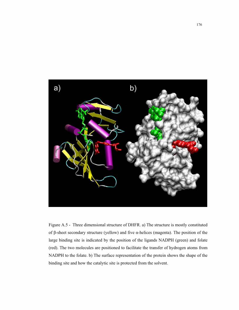
176

Figure A.5 - Three dimensional structure of DHFR. a) The structure is mostly constituted

of -sheet secondary structure (yellow) and five -helices (magenta). The position of the

large binding site is indicated by the position of the ligands NADPH (green) and folate

(red). The two molecules are positioned to facilitate the transfer of hydrogen atoms from

NADPH to the folate. b) The surface representation of the protein shows the shape of the

binding site and how the catalytic site is protected from the solvent.

177

DHFR is a monomeric protein with a relatively low molecular weight of

approximately 20 kDa. The structure of DHFR consists of 159 amino acid residues

which are mostly in a parallel -sheet conformation. Figure A.5 shows DHFR with -

helices in magenta and beta strands in yellow. The enzyme has a long binding site that

binds NADPH at one end and folate at the other. The two molecules are positioned in

such a way that transfer of hydrogen atoms from NADPH to the folate is facilitated.

This protein was chosen for this study due to its importance as a clinical target

and because it is known to undergo important conformational changes during the

binding and release of its substrates. NMR and kinetic studies have shown that DHFR

exists in two different unbound conformations (Schweitzer, Dicker et al. 1990; Feeney

2000). The comparison of experimental structures for the bound and unbound forms has

revealed structural differences (Cody, Galitsky et al. 1999). Recent computer

simulations have also shown that protein flexibility and loop motions were essential to

ligand binding, catalysis and release. Figure A.6 shows six different conformations

determined experimentally (Sawaya and Kraut 1997) using isomorphous crystal

structures for the catalytic cycle of DHFR. The conformations shown correspond to the

five detectable kinetic intermediates and to the transition state. These are the

holoenzyme, Michaelis complex, ternary product complex, tetrahydrofolate (THF)

binary complex, THF•NADPH complex and methotrexate-NADPH complex. Ligands

are shown for one of the structures to indentify the binding site. Arrows indicated the

regions near the binding site which display the largest amount of variation.

178

Figure A.6 – Conformational changes during the catalytic cycle of DHFR. The

conformations shown in tube representation correspond to the five detectable kinetic

intermediates and to the transition state. The location of the binding site is indicated by

the VDW representation of NADPH (green) and folate (red). Yellow arrows indicated

the regions near the binding site that display the largest amount of variation.

179

A.4. Maltose Binding Protein

Maltose binding protein exists in the periplasm of Gram-negative bacteria, plays

a fundamental role in active transport and also serves as a receptor for chemotaxis. This

protein is able to bind maltose, other linear maltodextrins, and cyclodextrins with high

affinity, but it binds glucose with low affinity. These maltooligosaccharides traverse the

outer bacterial membrane through specific channels (maltoporin LamB) and bind to

maltose binding protein. The bound protein then interacts with several components of

the cytoplasmatic membrane (MalF, MalG and two molecules of MalK) and initiates

the active transport of nutrients across the membrane by hydrolyzing ATP.

The three-dimensional structures of MBP, both bound (Spurlino, Lu et al. 1991)

and unbound (Sharff, Rodseth et al. 1992) to maltose, have been determined by X-ray

crystallography to 1.8 and 2.3 Å respectively. Maltose binding protein (shown in

Figures A.7 and A.8) is a monomeric protein with a molecular weight of 40.6 kDa. The

structure of this protein consists of two different globular domains that are separated by

a large cleft that forms the binding site. Upon ligand binding, the cleft region acts as an

hinge by bringing the two domains close together. The conformational change of

maltose binding protein upon addition of maltose has been detected in solution using

different experimental methods such as fluorescence (Szmelcman, Schwartz et al. 1976;

Hall, Gehring et al. 1997), electron paramagnetic resonance (Hall, Thorgeirsson et al.

1997), small-angle X-rayscattering (Shilton, Flocco et al. 1996), and NMR (Gehring,

Zhang et al. 1998). The large conformational rearrangement corresponds almost

exclusively to changes in the binding site region. The overall structures of the globular

180

domains stay mostly unchanged. This can be observed in Figure A.7 where the

structures of the bound and unbound forms are shown superimposed. The domain

displayed on the bottom was used for fitting using a least squares procedure. The

conformational rearrangement upon binding for this protein is the largest of all the

proteins used as models in this work. As shown in Figure A.7 the atomic displacements

for the residues shown at the top of the structure are approximately 15Å. In the

unbound form of this protein the binding cleft is exposed to the solvent. Due to the

large conformational rearrangement the ligand is engulfed in a tight binding cavity.

This dramatic change in solvent exposure of the binding site region is clearly visible in

Figure A.8. The binding motion in maltose binding protein is a critical part of its

function. Current models for the function of this protein (Duan, Hall et al. 2001)

postulate that the closed form of the protein is preferentially recognized by the

membrane components responsible for transport and chemotaxis functions.

Although this protein has not been used as a target for structure-based drug

design we decided to include maltose binding protein in this study in order to test the

dimensional reduction method with larger proteins that undergo large conformational

rearrangements.

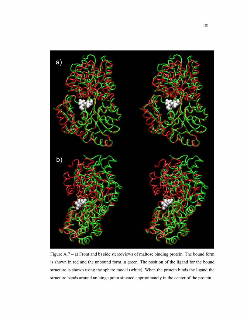
181

Figure A.7 – a) Front and b) side stereoviews of maltose binding protein. The bound form

is shown in red and the unbound form in green. The position of the ligand for the bound

structure is shown using the sphere model (white). When the protein binds the ligand the

structure bends around an hinge point situated approximately in the center of the protein.

182

Figure A.8 – Surface representation for the a) bound and b) unbound forms of maltose

binding protein (the ligand is shown in the unbound form for comparison purposes). After

binding maltose the two domains close around a hinge in the center of the protein and

change the solvent exposure of the binding site.

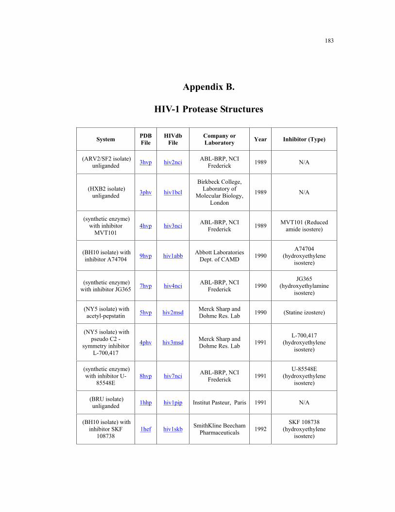
183

Appendix B.

HIV-1 Protease Structures

System PDB

File

HIVdb

File

Company or

Laboratory Year Inhibitor (Type)

(ARV2/SF2 isolate)

unliganded 3hvp hiv2nci

ABL-BRP, NCI

Frederick 1989 N/A

(HXB2 isolate)

unliganded 3phv hiv1bcl

Birkbeck College,

Laboratory of

Molecular Biology,

London

1989 N/A

(synthetic enzyme)

with inhibitor

MVT101

4hvp hiv3nciABL-BRP, NCI

Frederick 1989

MVT101 (Reduced

amide isostere)

(BH10 isolate) with

inhibitor A74704 9hvp hiv1abb

Abbott Laboratories

Dept. of CAMD 1990

A74704

(hydroxyethylene

isostere)

(synthetic enzyme)

with inhibitor JG365 7hvp hiv4nci

ABL-BRP, NCI

Frederick 1990

JG365

(hydroxyethylamine

isostere)

(NY5 isolate) with

acetyl-pepstatin5hvp hiv2msd

Merck Sharp and

Dohme Res. Lab 1990 (Statine izostere)

(NY5 isolate) with

pseudo C2 -

symmetry inhibitor

L-700,417

4phv hiv3msdMerck Sharp and

Dohme Res. Lab 1991

L-700,417

(hydroxyethylene

isostere)

(synthetic enzyme)

with inhibitor U-

85548E

8hvp hiv7nciABL-BRP, NCI

Frederick 1991

U-85548E

(hydroxyethylene

isostere)

(BRU isolate)

unliganded 1hhp hiv1pip Institut Pasteur, Paris 1991 N/A

(BH10 isolate) with

inhibitor SKF

108738

1hef hiv1skbSmithKline Beecham

Pharmaceuticals 1992

SKF 108738

(hydroxyethylene

isostere)

184

System PDB

File

HIVdb

File

Company or

Laboratory Year Inhibitor (Type)

(BH10 isolate) with

inhibitor SKF

107457

1heg hiv2skbSmithKline Beecham

Pharmaceuticalss 1992

SKF 107457

(hydroxyethylene

isostere)

(BH10 isolate) with

hydroxyethylene

inhibitor

1aaq hiv3skbSmithKline Beecham

Pharmaceuticalss 1992

(hydroxyethylene

isostere)

(isolate unknown)

with

dihydroxyethylene

inhibitor U75875

1hiv hiv8nciABL-BRP, NCI

Frederick 1992

U75875

(dihydroxyethylene

isostere)

(BH10 isolate) with

C2 - symmetric

phosphinate

inhibitor

1hos hiv4skbSmithKline Beecham

Pharmaceuticalss 1993

SB204144 (perfectly

symmetrical

phosphinate inhibitor)

(BH10 isolate) with

penicillin - derived

C2 - symmetric

inhibitor

1hte hiv1glxGlaxo Group

Research Limited 1993

GR123976 (penicillin-

derived C2-symmetric

inhibitor)

(BH10 isolate) with

penicillin - derived

C2 - symmetric

inhibitor

1htf hiv2glxGlaxo Group

Research Limited 1993

GR126045 (penicillin-

derived C2-symmetric

inhibitor)

(BH10 isolate) with

inhibitor SB206343 1hps hiv6skb

SmithKline Beecham

Pharmaceuticalss 1994

SB 206343

(hydroxyethylene

isostere)

(NY5 isolate) with

inhibitor L-735,524

(MK639)

[CRIXIVAN

(Indinavir)]

1hsg hiv4msd Merck & Co., Inc. 1994

L-735,524; MK-639,

Indinavir,Crixivan

(hydroxyethylene

isostere)

(BH10 isolate) with

inhibitor SB 203386 1sbg hiv7skb

SmithKline Beecham

Pharmaceuticalss 1994

SB 203386

(hydroxyethylene

isostere)

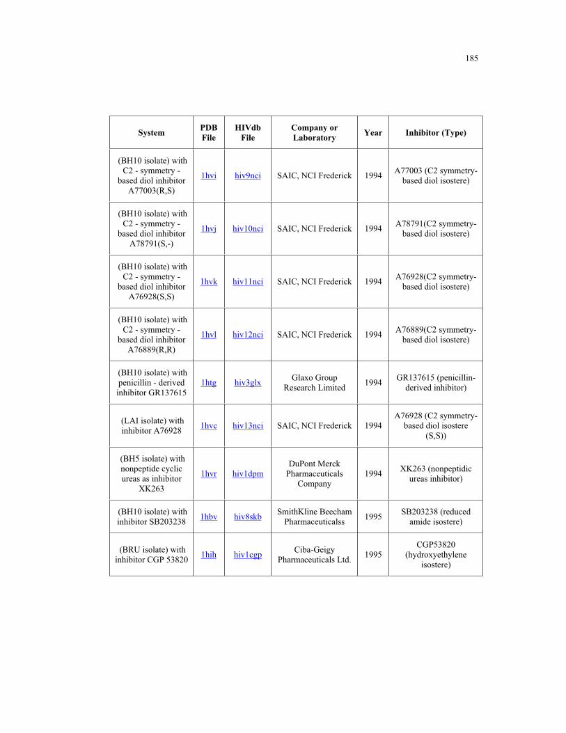
185

System PDB

File

HIVdb

File

Company or

Laboratory Year Inhibitor (Type)

(BH10 isolate) with

C2 - symmetry -

based diol inhibitor

A77003(R,S)

1hvi hiv9nci SAIC, NCI Frederick 1994 A77003 (C2 symmetry-

based diol isostere)

(BH10 isolate) with

C2 - symmetry -

based diol inhibitor

A78791(S,-)

1hvj hiv10nci SAIC, NCI Frederick 1994 A78791(C2 symmetry-

based diol isostere)

(BH10 isolate) with

C2 - symmetry -

based diol inhibitor

A76928(S,S)

1hvk hiv11nci SAIC, NCI Frederick 1994 A76928(C2 symmetry-

based diol isostere)

(BH10 isolate) with

C2 - symmetry -

based diol inhibitor

A76889(R,R)

1hvl hiv12nci SAIC, NCI Frederick 1994 A76889(C2 symmetry-

based diol isostere)

(BH10 isolate) with

penicillin - derived

inhibitor GR137615

1htg hiv3glxGlaxo Group

Research Limited 1994

GR137615 (penicillin-

derived inhibitor)

(LAI isolate) with

inhibitor A76928 1hvc hiv13nci SAIC, NCI Frederick 1994

A76928 (C2 symmetry-

based diol isostere

(S,S))

(BH5 isolate) with

nonpeptide cyclic

ureas as inhibitor

XK263

1hvr hiv1dpm

DuPont Merck

Pharmaceuticals

Company

1994 XK263 (nonpeptidic

ureas inhibitor)

(BH10 isolate) with

inhibitor SB203238 1hbv hiv8skb

SmithKline Beecham

Pharmaceuticalss 1995

SB203238 (reduced

amide isostere)

(BRU isolate) with

inhibitor CGP 53820 1hih hiv1cgp

Ciba-Geigy

Pharmaceuticals Ltd. 1995

CGP53820

(hydroxyethylene

isostere)

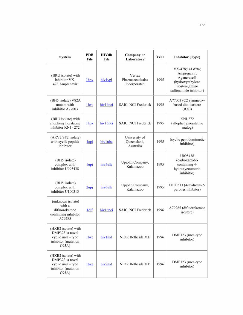
186

System PDB

File

HIVdb

File

Company or

Laboratory Year Inhibitor (Type)

(BRU isolate) with

inhibitor VX-

478,Amprenavir

1hpv hiv1vpi

Vertex

Pharmaceuticalss

Incorporated

1995

VX-478;141W94;

Amprenavir;

Agenerase®

(hydroxyethylene

isostere,amino

sulfonamide inhibitor)

(BH5 isolate) V82A

mutant with

inhibitor A77003

1hvs hiv14nci SAIC, NCI Frederick 1995

A77003 (C2 symmetry-

based diol isostere

(R,S))

(BRU isolate) with

allophenylnorstatine

inhibitor KNI - 272

1hpx hiv15nci SAIC, NCI Frederick 1995

KNI-272

(allophenylnorstatine

analog)

(ARV2/SF2 isolate)

with cyclic peptide

inhibitor

1cpi hiv1uba

University of

Queensland,

Australia

1995 (cyclic peptidomimetic

inhibitor)

(BH5 isolate)

complex with

inhibitor U095438

1upj hiv5ulkUpjohn Company,

Kalamazoo 1995

U095438

(carboxamide-

containing 4-

hydroxycoumarin

inhibitor)

(BH5 isolate)

complex with

inhibitor U100313

2upj hiv6ulkUpjohn Company,

Kalamazoo 1995

U100313 (4-hydroxy-2-

pyrones inhibitor)

(unknown isolate)

with a

difluoroketone

containing inhibitor

A79285

1dif hiv16nci SAIC, NCI Frederick 1996 A79285 (difluoroketone

isostere)

(HXB2 isolate) with

DMP323, a novel

cyclic urea - type

inhibitor (mutation

C95A)

1bve hiv1nid NIDR Bethesda,MD 1996 DMP323 (urea-type

inhibitor)

(HXB2 isolate) with

DMP323, a novel

cyclic urea - type

inhibitor (mutation

C95A)

1bvg hiv2nid NIDR Bethesda,MD 1996 DMP323 (urea-type

inhibitor)

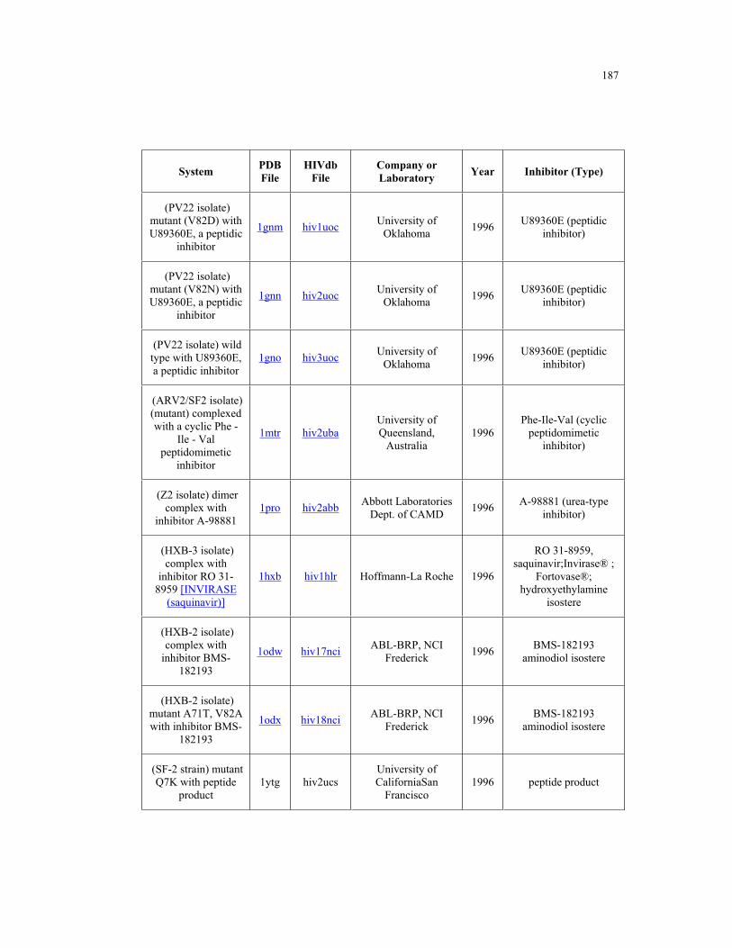
187

System PDB

File

HIVdb

File

Company or

Laboratory Year Inhibitor (Type)

(PV22 isolate)

mutant (V82D) with

U89360E, a peptidic

inhibitor

1gnm hiv1uocUniversity of

Oklahoma 1996

U89360E (peptidic

inhibitor)

(PV22 isolate)

mutant (V82N) with

U89360E, a peptidic

inhibitor

1gnn hiv2uocUniversity of

Oklahoma 1996

U89360E (peptidic

inhibitor)

(PV22 isolate) wild

type with U89360E,

a peptidic inhibitor

1gno hiv3uocUniversity of

Oklahoma 1996

U89360E (peptidic

inhibitor)

(ARV2/SF2 isolate)

(mutant) complexed

with a cyclic Phe -

Ile - Val

peptidomimetic

inhibitor

1mtr hiv2uba

University of

Queensland,

Australia

1996

Phe-Ile-Val (cyclic

peptidomimetic

inhibitor)

(Z2 isolate) dimer

complex with

inhibitor A-98881

1pro hiv2abbAbbott Laboratories

Dept. of CAMD 1996

A-98881 (urea-type

inhibitor)

(HXB-3 isolate)

complex with

inhibitor RO 31-

8959 [INVIRASE

(saquinavir)]

1hxb hiv1hlr Hoffmann-La Roche 1996

RO 31-8959,

saquinavir;Invirase® ;

Fortovase®;

hydroxyethylamine

isostere

(HXB-2 isolate)

complex with

inhibitor BMS-

182193

1odw hiv17nciABL-BRP, NCI

Frederick 1996

BMS-182193

aminodiol isostere

(HXB-2 isolate)

mutant A71T, V82A

with inhibitor BMS-

182193

1odx hiv18nciABL-BRP, NCI

Frederick 1996

BMS-182193

aminodiol isostere

(SF-2 strain) mutant

Q7K with peptide

product

1ytg hiv2ucs

University of

CaliforniaSan

Francisco

1996 peptide product

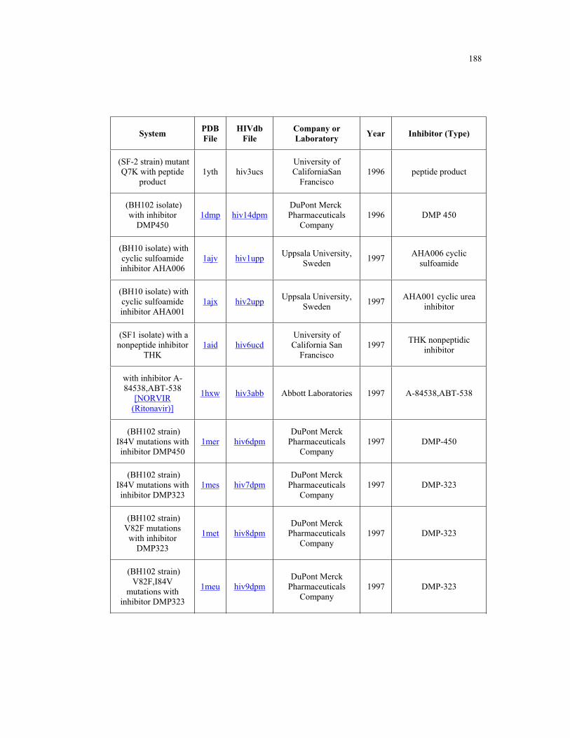
188

System PDB

File

HIVdb

File

Company or

Laboratory Year Inhibitor (Type)

(SF-2 strain) mutant

Q7K with peptide

product

1yth hiv3ucs

University of

CaliforniaSan

Francisco

1996 peptide product

(BH102 isolate)

with inhibitor

DMP450

1dmp hiv14dpm

DuPont Merck

Pharmaceuticals

Company

1996 DMP 450

(BH10 isolate) with

cyclic sulfoamide

inhibitor AHA006

1ajv hiv1uppUppsala University,

Sweden 1997

AHA006 cyclic

sulfoamide

(BH10 isolate) with

cyclic sulfoamide

inhibitor AHA001

1ajx hiv2uppUppsala University,

Sweden 1997

AHA001 cyclic urea

inhibitor

(SF1 isolate) with a

nonpeptide inhibitor

THK

1aid hiv6ucd

University of

California San

Francisco

1997 THK nonpeptidic

inhibitor

with inhibitor A-

84538,ABT-538

[NORVIR

(Ritonavir)]

1hxw hiv3abb Abbott Laboratories 1997 A-84538,ABT-538

(BH102 strain)

I84V mutations with

inhibitor DMP450

1mer hiv6dpm

DuPont Merck

Pharmaceuticals

Company

1997 DMP-450

(BH102 strain)

I84V mutations with

inhibitor DMP323

1mes hiv7dpm

DuPont Merck

Pharmaceuticals

Company

1997 DMP-323

(BH102 strain)

V82F mutations

with inhibitor

DMP323

1met hiv8dpm

DuPont Merck

Pharmaceuticals

Company

1997 DMP-323

(BH102 strain)

V82F,I84V

mutations with

inhibitor DMP323

1meu hiv9dpm

DuPont Merck

Pharmaceuticals

Company

1997 DMP-323

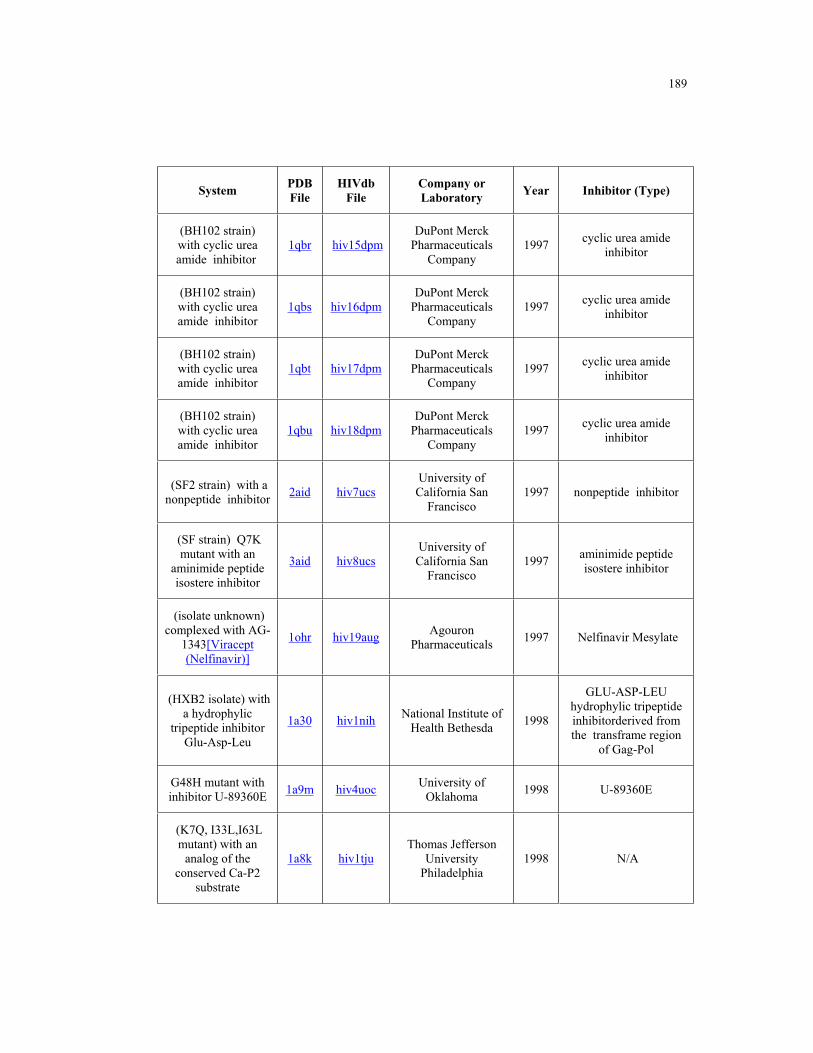
189

System PDB

File

HIVdb

File

Company or

Laboratory Year Inhibitor (Type)

(BH102 strain)

with cyclic urea

amide inhibitor

1qbr hiv15dpm

DuPont Merck

Pharmaceuticals

Company

1997 cyclic urea amide

inhibitor

(BH102 strain)

with cyclic urea

amide inhibitor

1qbs hiv16dpm

DuPont Merck

Pharmaceuticals

Company

1997 cyclic urea amide

inhibitor

(BH102 strain)

with cyclic urea

amide inhibitor

1qbt hiv17dpm

DuPont Merck

Pharmaceuticals

Company

1997 cyclic urea amide

inhibitor

(BH102 strain)

with cyclic urea

amide inhibitor

1qbu hiv18dpm

DuPont Merck

Pharmaceuticals

Company

1997 cyclic urea amide

inhibitor

(SF2 strain) with a

nonpeptide inhibitor 2aid hiv7ucs

University of

California San

Francisco

1997 nonpeptide inhibitor

(SF strain) Q7K

mutant with an

aminimide peptide

isostere inhibitor

3aid hiv8ucs

University of

California San

Francisco

1997 aminimide peptide

isostere inhibitor

(isolate unknown)

complexed with AG-

1343[Viracept

(Nelfinavir)]

1ohr hiv19augAgouron

Pharmaceuticals 1997 Nelfinavir Mesylate

(HXB2 isolate) with

a hydrophylic

tripeptide inhibitor

Glu-Asp-Leu

1a30 hiv1nihNational Institute of

Health Bethesda 1998

GLU-ASP-LEU

hydrophylic tripeptide

inhibitorderived from

the transframe region

of Gag-Pol

G48H mutant with

inhibitor U-89360E 1a9m hiv4uoc

University of

Oklahoma 1998 U-89360E

(K7Q, I33L,I63L

mutant) with an

analog of the

conserved Ca-P2

substrate

1a8k hiv1tju

Thomas Jefferson

University

Philadelphia

1998 N/A

190

System PDB

File

HIVdb

File

Company or

Laboratory Year Inhibitor (Type)

T31S, V32I, L33V,

E34A, E35G, M36I,

S37E mutations with

inhibitor SB203386

1bdl hiv10skbSmithKline Beecham

Pharmaceuticalss 1998 SB203386

T31S, V32I, L33V,

E34A, E35G, M36I,

S37E, I47V,V82I

mutations with

inhibitor SB203386

1bdq hiv11skbSmithKline Beecham

Pharmaceuticalss 1998 SB203386

T31S, L33V, E34T,

E35G, M36I, S37E

mutations with

inhibitor SB203386

1bdr hiv12skbSmithKline Beecham

Pharmaceuticalss 1998 SB203386

(BH102 strain)

I82F, C95A

mutations with

inhibitor SD146

1bv7 hiv10dpm

DuPont Merck

Pharmaceuticals

Company

1998 SD146

(BH102 strain)

I84V,C95A

mutations with

inhibitor XV638

(cyclic urea

inhibitor)

1bv9 hiv11dpm

DuPont Merck

Pharmaceuticals

Company

1998 XV638

V82F, I84V

mutations with

inhibitor XV638

(cyclic urea

inhibitor)

1bwa hiv12dpm

DuPont Merck

Pharmaceuticals

Company

1998 XV638

(BH102 strain)

V82F, I84V

mutations with

inhibitor SD146

1bwb hiv13dpm

DuPont

MerckPharmaceutical

sCompany

1998 SD146

A28S mutant, with

inhibitor U89360E 1axa hiv5uoc

University of

Oklahoma 1999 U89360E

(BH102 strain)

with inhibitor Q8261 1hvh hiv19dpm

DuPont Merck

Pharmaceuticals

Company

1999

Q8261, Nonpeptide

Cyclic

Cyanoguanidines

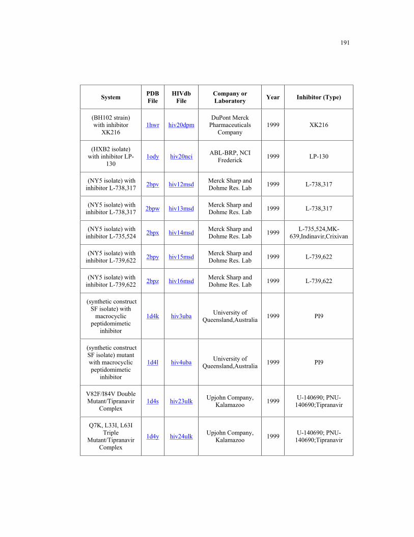
191

System PDB

File

HIVdb

File

Company or

Laboratory Year Inhibitor (Type)

(BH102 strain)

with inhibitor

XK216

1hwr hiv20dpm

DuPont Merck

Pharmaceuticals

Company

1999 XK216

(HXB2 isolate)

with inhibitor LP-

130

1ody hiv20nciABL-BRP, NCI

Frederick 1999 LP-130

(NY5 isolate) with

inhibitor L-738,317 2bpv hiv12msd

Merck Sharp and

Dohme Res. Lab 1999 L-738,317

(NY5 isolate) with

inhibitor L-738,317 2bpw hiv13msd

Merck Sharp and

Dohme Res. Lab 1999 L-738,317

(NY5 isolate) with

inhibitor L-735,524 2bpx hiv14msd

Merck Sharp and

Dohme Res. Lab 1999

L-735,524,MK-

639,Indinavir,Crixivan

(NY5 isolate) with

inhibitor L-739,622 2bpy hiv15msd

Merck Sharp and

Dohme Res. Lab 1999 L-739,622

(NY5 isolate) with

inhibitor L-739,622 2bpz hiv16msd

Merck Sharp and

Dohme Res. Lab 1999 L-739,622

(synthetic construct

SF isolate) with

macrocyclic

peptidomimetic

inhibitor

1d4k hiv3ubaUniversity of

Queensland,Australia 1999 PI9

(synthetic construct

SF isolate) mutant

with macrocyclic

peptidomimetic

inhibitor

1d4l hiv4ubaUniversity of

Queensland,Australia 1999 PI9

V82F/I84V Double

Mutant/Tipranavir

Complex

1d4s hiv23ulk Upjohn Company,

Kalamazoo 1999

U-140690; PNU-

140690;Tipranavir

Q7K, L33I, L63I

Triple

Mutant/Tipranavir

Complex

1d4y hiv24ulk Upjohn Company,

Kalamazoo 1999

U-140690; PNU-

140690;Tipranavir

192

System PDB

File

HIVdb

File

Company or

Laboratory Year Inhibitor (Type)

(isolate unknown)

with inhibitor RO31-

8558

N/A hiv2hlr Hoffmann-La Roche 1991

RO31-8558

hydroxyethylamine

isostere

(isolate unknown)

with inhibitor

AG1001

N/A hiv1augAgouron

Pharmaceuticals 1991 AG1001

(isolate unknown)

with inhibitor

AG1002

N/A hiv2augAgouron

Pharmaceuticals 1991 AG1002

(isolate unknown)

with inhibitor

AG1004

N/A hiv3augAgouron

Pharmaceuticals 1991 AG1004

(isolate unknown)

with inhibitor

LILLY765

N/A hiv1lll Lilly Pharmaceuticals 1991 LILLY765

(isolate unknown)

with inhibitor I-

BMS-01

N/A hiv1bms Bristol-Myers Squibb 1993 I-BMS-01

(isolate unknown)

with inhibitor I-

BMS-02

N/A hiv2bms Bristol-Myers Squibb 1993 I-BMS-02

mutant C95A

(BH102 isolate) with

inhibitor DMP323

N/A hiv2dpm

DuPont Merck

Pharmaceuticals

Company

1996 DMP323 urea based

inhibitor

mutant C95A

(BH102 isolate) with

inhibitor Q8467

N/A hiv3dpm

DuPont Merck

Pharmaceuticals

Company

1997 Q8467 cyclic urea amid

inhibitor

mutant C95A

(BH102 isolate) with

inhibitor XV638

N/A hiv4dpm

DuPont Merck

Pharmaceuticals

Company

1997 XV638 cyclic urea

amid inhibitor

mutant C95A

(BH102 isolate) with

inhibitor SD146

N/A hiv5dpm

DuPont Merck

Pharmaceuticals

Company

1997 SD146 cyclic urea amid

inhibitor

193

System PDB

File

HIVdb

File

Company or

Laboratory Year Inhibitor (Type)

(isolate unknown)

with inhibitor N/A hiv4glx

Glaxo Group

Research Limited 1991 GR-XXXX

(ROD isolate) with

inhibitor L-689,502 N/A hiv7msd

Merck Sharp and

Dohme Res. Lab 1992 L-689,502

(BH-10 isolate)

with inhibitor MDL

104,168

N/A hiv1mmd MMDRI, France 1993

MDL 104,168

difluorostatone

inhibitor

(BH-10 isolate)

with inhibitor MDL

73,669

N/A hiv2mmd MMDRI, France 1993

MDL 73,669

difluorostatone

inhibitor

(BH-10 isolate)

with inhibitor MDL

73,730

N/A hiv3mmd MMDRI, France 1993

MDL 73,730

difluorostatone

inhibitor

(BH-10 isolate)

with inhibitor MDL

73,881

N/A hiv4mmd MMDRI, France 1993

MDL 73,881

difluorostatone

inhibitor

(BH-10 isolate)

with inhibitor MDL

73,915

N/A hiv5mmd MMDRI, France 1993

MDL 73,915

difluorostatone

inhibitor

(BH-10 isolate) with

inhibitor MDL

74,538

N/A hiv6mmd MMDRI, France 1993

MDL

74,538difluorostatone

inhibitor

(BH-10 isolate) with

inhibitor MDL

75,635

N/A hiv7mmd MMDRI, France 1993

MDL

75,635difluorostatone

inhibitor

(BH-10 isolate) with

inhibitor MDL

75,305

N/A hiv8mmd MMDRI, France 1993

MDL

75,305difluorostatone

inhibitor

(BH-10 isolate)

with inhibitor

AHA004

N/A hiv3uppUppsala University,

Sweden 1997

AHA004 cyclic urea

inhibitor

(BH-10 isolate)

with inhibitor

AHA009

N/A hiv4uppUppsala University,

Sweden 1997

AHA009 sulfoamide

inhibitor

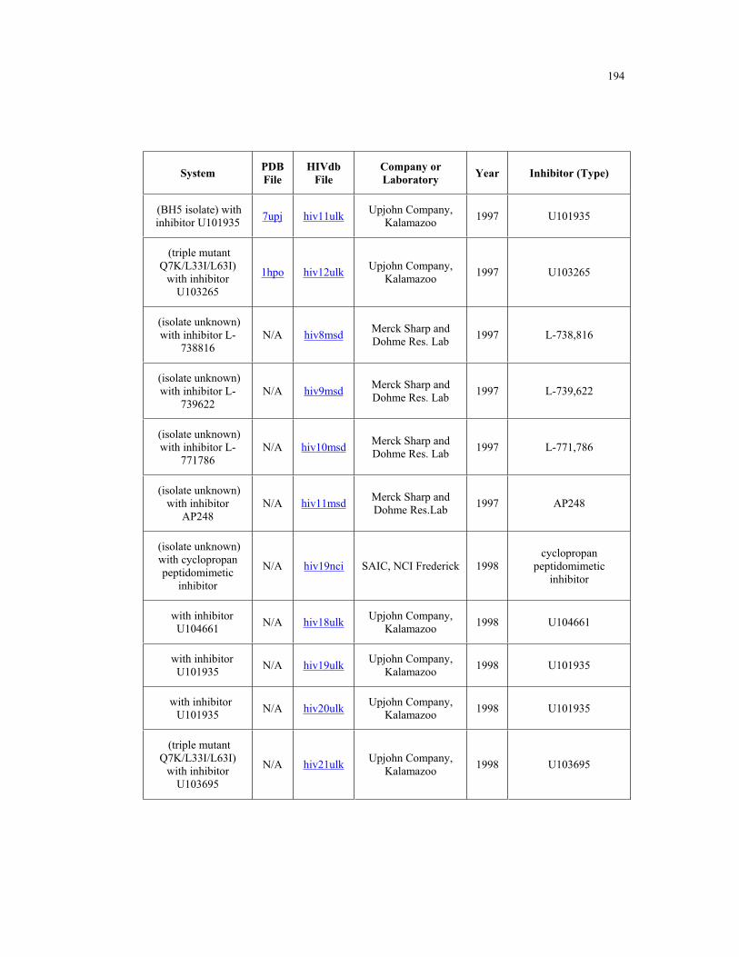
194

System PDB

File

HIVdb

File

Company or

Laboratory Year Inhibitor (Type)

(BH5 isolate) with

inhibitor U101935 7upj hiv11ulk

Upjohn Company,

Kalamazoo 1997 U101935

(triple mutant

Q7K/L33I/L63I)

with inhibitor

U103265

1hpo hiv12ulkUpjohn Company,

Kalamazoo 1997 U103265

(isolate unknown)

with inhibitor L-

738816

N/A hiv8msdMerck Sharp and

Dohme Res. Lab 1997 L-738,816

(isolate unknown)

with inhibitor L-

739622

N/A hiv9msdMerck Sharp and

Dohme Res. Lab 1997 L-739,622

(isolate unknown)

with inhibitor L-

771786

N/A hiv10msdMerck Sharp and

Dohme Res. Lab 1997 L-771,786

(isolate unknown)

with inhibitor

AP248

N/A hiv11msdMerck Sharp and

Dohme Res.Lab 1997 AP248

(isolate unknown)

with cyclopropan

peptidomimetic

inhibitor

N/A hiv19nci SAIC, NCI Frederick 1998

cyclopropan

peptidomimetic

inhibitor

with inhibitor

U104661 N/A hiv18ulk

Upjohn Company,

Kalamazoo 1998 U104661

with inhibitor

U101935 N/A hiv19ulk

Upjohn Company,

Kalamazoo 1998 U101935

with inhibitor

U101935 N/A hiv20ulk

Upjohn Company,

Kalamazoo 1998 U101935

(triple mutant

Q7K/L33I/L63I)

with inhibitor

U103695

N/A hiv21ulkUpjohn Company,

Kalamazoo 1998 U103695

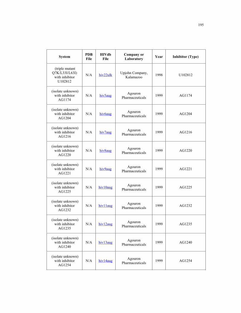
195

System PDB

File

HIVdb

File

Company or

Laboratory Year Inhibitor (Type)

(triple mutant

Q7K/L33I/L63I)

with inhibitor

U102812

N/A hiv22ulkUpjohn Company,

Kalamazoo 1998 U102812

(isolate unknown)

with inhibitor

AG1174

N/A hiv5augAgouron

Pharmaceuticals 1999 AG1174

(isolate unknown)

with inhibitor

AG1204

N/A hiv6augAgouron

Pharmaceuticals 1999 AG1204

(isolate unknown)

with inhibitor

AG1216

N/A hiv7augAgouron

Pharmaceuticals 1999 AG1216

(isolate unknown)

with inhibitor

AG1220

N/A hiv8augAgouron

Pharmaceuticals 1999 AG1220

(isolate unknown)

with inhibitor

AG1221

N/A hiv9augAgouron

Pharmaceuticals 1999 AG1221

(isolate unknown)

with inhibitor

AG1225

N/A hiv10augAgouron

Pharmaceuticals 1999 AG1225

(isolate unknown)

with inhibitor

AG1232

N/A hiv11augAgouron

Pharmaceuticals 1999 AG1232

(isolate unknown)

with inhibitor

AG1235

N/A hiv12augAgouron

Pharmaceuticals 1999 AG1235

(isolate unknown)

with inhibitor

AG1240

N/A hiv13augAgouron

Pharmaceuticals 1999 AG1240

(isolate unknown)

with inhibitor

AG1254

N/A hiv14augAgouron

Pharmaceuticals 1999 AG1254

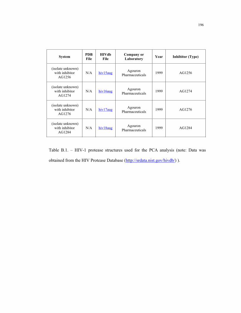
196

System PDB

File

HIVdb

File

Company or

Laboratory Year Inhibitor (Type)

(isolate unknown)

with inhibitor

AG1256

N/A hiv15augAgouron

Pharmaceuticals 1999 AG1256

(isolate unknown)

with inhibitor

AG1274

N/A hiv16augAgouron

Pharmaceuticals 1999 AG1274

(isolate unknown)

with inhibitor

AG1276

N/A hiv17augAgouron

Pharmaceuticals 1999 AG1276

(isolate unknown)

with inhibitor

AG1284

N/A hiv18augAgouron

Pharmaceuticals 1999 AG1284

Table B.1. – HIV-1 protease structures used for the PCA analysis (note: Data was

obtained from the HIV Protease Database (http://srdata.nist.gov/hivdb/) ).

197

Appendix C.

Molecular Modeling and Rigid Protein Docking

C.1. Molecular Modeling

A molecule is characterized by a pair (A; B), in which A represents a collection

of atoms, and B represents a collection of bonds between pairs of atoms. Information

used for kinematic and energy computations is associated with each of the atoms and

bonds. Each atom carries standard information, such as its van der Waals radius. Three

pieces of information are associated with each bond: (i) bond length, is the distance

between atom centers; (ii) bond angle, is the angle between two consecutive bonds; (iii)

whether the bond is rotatable or not. Since bond lengths and angles do not change

significantly, it is common practice to consider them fixed. Thus the degrees of

freedom of the molecule arise from the rotatable bonds. The three dimensional

embedding of a molecule defined when we assign values to its rotatable bonds is called

the conformation of the molecule. Ligands typically have 3-15 rotatable bonds, while

receptors have 1,000-2,000 rotatable bonds. The dimension of the combined search

space makes the docking problem computationally intractable.

One key aspect of molecular modeling is calculating the energy of

conformations and interactions. This energy can be calculated with a wide range of

methods ranging from quantum mechanics to purely empirical energy functions. The

accuracy of these functions is usually proportional to its computational expense and

198

choosing the correct energy calculation method is highly dependent on the application.

Computation times for different methods can range from a few milliseconds on a

workstation to several days on a supercomputer.

In the context of docking, energy evaluations are usually carried out with the

help of a scoring function and developing these is a major challenge facing structure

based drug design (Vieth, Hirst et al. 1998; Muegge and Rarey 2001; Halperin, Ma et

al. 2002). No matter how efficient and accurate the geometric modeling of the binding

process is, without good scoring functions it is impossible to obtain correct solutions.

The two main characteristics of a good scoring function are selectivity and efficiency.

Selectivity enables the function to distinguish between correctly and incorrectly docked

structures and efficiency enables the docking program to run in a reasonable amount of

time.

A large number of current scoring functions are based on forcefields that were

initially designed to simulate the function of proteins (Cornell, Cieplak et al. 1995;

MacKerell, Bashford et al. 1998). A forcefield is an empirical fit to the potential energy

surface in which the protein exists and is obtained by establishing a model with a

combination of bonded terms (bond distances, bond angles, torsional angles, etc.) and

non-bonded terms (van der Waals and electrostatic). The relative contributions of these

terms are adjusted for the different types of atoms in the simulated molecule by

adjusting a series of empirical parameters. Some scoring functions used in molecular

docking have been adapted to include terms such as solvation and entropy (Morris,

199

Goodsell et al. 1998). A separate approach is to use statistical scoring functions that are

derived using experimental data (Muegge and Martin 1999).

C.2. Rigid Protein Docking

Most of the docking methods used at the present moment in academic and

industrial research assume a rigid protein. To illustrate the methodology used by these

methods we will briefly discuss three of the most common programs used for docking:

Autodock (Morris, Goodsell et al. 1998), Dock (Ewing and Kuntz 1997) and FlexX

(Kramer, Rarey et al. 1999).

Autodock uses a kinematic model for the ligand based on rotations around

single bonds. The ligand begins the search process randomly outside the binding site

and by exploring the values for translations, rotations and its internal degrees of

freedom, it will eventually reach the bound conformation. Distinction between good

and bad docked conformations is carried out by the scoring function. Autodock is able

to use Monte Carlo methods or simulated annealing (SA) in the search process and in

its last version introduced the ability to use genetic algorithms (GA). The routine

implemented in the recent release is a Lamarkian genetic algorithm (LGA), in which a

traditional GA is used for global search and is combined with a Solis and Wets local

search procedure. Morris et al show that the new LGA is able to handle ligands with a

larger number of degrees of freedom than SA or traditional GA.

FlexX and Dock both use an incremental construction algorithm which attempts

to reconstruct the bound ligand by first placing a rigid anchor in the binding site and

200

later using a greedy algorithm to add fragments and complete the ligand structure.

Although these programs are more efficient than Autodock in the sense that they

require fewer energy evaluations there exist some tradeoffs. One of main problems is

that it is not trivial to choose the anchor fragment and its choice will determine what

solutions can be obtained. Also the greedy algorithm propagates errors resulting from

initial bad choices that lead to missing final conformations of lower energy.

In order to solve the docking problem conformation methods using standard robotics

techniques such as probabilistic roadmap planning have been recently described[8,9]

. In

addition to being successful in finding the correct docking conformation these methods

are useful in identifying possible binding sites and in providing a computational

efficient description of the dynamics of ligand binding.

201

References

Abseher, R. and Nilges, M. (1998). "Are there non-trivial dynamic cross-correlations in

proteins?" Journal of Molecular Biology 279(4): 911-20.

Abseher, R. and Nilges, M. (2000). "Efficient sampling in collective coordinate space."

Proteins: Structure, Function, and Genetics 39(1): 82-8.

Althaus, E., Kohlbacher, O., Lenhof, H. P. and Muller, P. (2002). "A combinatorial

approach to protein docking with flexible side chains." Journal of

Computational Biology 9(4): 597-612.

Amadei, A., Ceruso, M. A. and Di Nola, A. (1999). "On the convergence of the

conformational coordinates basis set obtained by the essential dynamics analysis

of proteins' molecular dynamics simulations." Proteins: Structure, Function, and

Genetics 36(4): 419-24.

Amadei, A., Linssen, A. B. and Berendsen, H. J. (1993). "Essential dynamics of

proteins." Proteins: Structure, Function, and Genetics 17(4): 412-25.

202

Amadei, A., Linssen, A. B., de Groot, B. L., van Aalten, D. M. and Berendsen, H. J.

(1996). "An efficient method for sampling the essential subspace of proteins."

Journal of Biomolecular Structure and Dynamics 13(4): 615-25.

Amit, A. G., Mariuzza, R. A., Phillips, S. E. and Poljak, R. J. (1986). "Three-

dimensional structure of an antigen-antibody complex at 2.8 A resolution."

Science 233(4765): 747-53.

Anderson, A. C., O'Neil, R. H., Surti, T. S. and Stroud, R. M. (2001). "Approaches to

solving the rigid receptor problem by identifying a minimal set of flexible

residues during ligand docking." Chemical Biology 8(5): 445-57.

Andrews, B. K., Romo, T., Clarage, J. B., Pettitt, B. M. and Phillips, G. N., Jr. (1998).

"Characterizing global substates of myoglobin." Structure 6(5): 587-94.

Apostolakis, J., Pluckthun, A. and Caflisch, A. (1998). "Docking small ligands in

flexible binding sites." Journal of Computational Chemistry 19(1): 21-37.

Appelt, K. (1993). "Crystal structures of HIV-1 protease-inhibitor complexes."

Perspectives in Drug Discovery and Design 1: 23–48.

203

Auzat, I., Gawlita, E. and Garel, J. R. (1995). "Slow ligand-induced transitions in the

allosteric phosphofructokinase from Escherichia coli." Journal of Molecular

Biology 249(2): 478-92.

Bahar, I., Erman, B., Jernigan, R. L., Atilgan, A. R. and Covell, D. G. (1999).

"Collective motions in HIV-1 reverse transcriptase: examination of flexibility

and enzyme function." Journal of Molecular Biology 285(3): 1023-37.

Banner, D. W. and Hadvary, P. (1991). "Crystallographic analysis at 3.0-A resolution

of the binding to human thrombin of four active site-directed inhibitors."

Journal of Biological Chemistry 266(30): 20085-93.

Berendsen, H. J. C., Postma, J. P. M., van Gunsteren, W. F., DiNola, A. and Haak, J. R.

(1984). "Molecular dynamics with coupling to an external bath." Journal of

Chemical Physics 81(8): 3684-3690.

Berg, B. A. and Neuhaus, T. (1992). "Multicanonical ensemble: A new approach to

simulate first-order phase transitions." Physical Review Letters 68: 9-12.

Berman, H. M., Westbrook, J., Feng, Z., Gilliland, G., Bhat, T. N., Weissig, H.,

Shindyalov, I. N. and Bourne, P. E. (2000). "The Protein Data Bank." Nucleic

Acids Research 28(1): 235-242.

204

Betts, M. J. and Sternberg, M. J. (1999). "An analysis of conformational changes on

protein-protein association: implications for predictive docking." Protein

Engineering 12(4): 271-83.

Bishop, C. M., Svensen, M. and Williams, C. K. (1998). "GTM:the Generative

Topographic Mapping." Neural Computation 10(1): 215 -234.

Blow, D. M. (1976). "Structure and Mechanism of Chymotrypsin." Accounts Chemical

Research 9: 145-152.

Bolin, J. T., Filman, D. J., Matthews, D. A., Hamlin, R. C. and Kraut, J. (1982).

"Crystal structures of Escherichia coli and Lactobacillus casei dihydrofolate

reductase refined at 1.7 A resolution. I. General features and binding of

methotrexate." Journal of Biological Chemistry 257(22): 13650-62.

Borhani, D. W., Harter, T. M. and Petrash, J. M. (1992). "The crystal structure of the

aldose reductase.NADPH binary complex." Journal of Biological Chemistry

267(34): 24841-7.

Bouzida, D., Rejto, P. A., Arthurs, S., Colson, A. B., Freer, S. T., Gehlhaar, D. K.,

Larson, V., Luty, B. A., Rose, P. W. and Verkhivker, G. M. (1999). "Computer

simulations of ligand-protein binding with ensembles of protein conformations:

205

A Monte Carlo study of HIV-1 protease binding energy landscapes."

International Journal of Quantum Chemistry 72: 73-84.

Brooks, C. L. I., Montgomery, B. and Karplus, M. (1988). Proteins : A Theoretical

Perspective of Dynamics, Structure and Thermodynamics. New York, John

Wiley & Sons.

Broughton, H. B. (2000). "A method for including protein flexibility in protein-ligand

docking: improving tools for database mining and virtual screening." Journal of

Molecular Graphics and Modeling 18(3): 247-57, 302-4.

Bruccoleri, R. E. and Karplus, M. (1990). "Conformational sampling using high-

temperature molecular dynamics." Biopolymers 29(14): 1847-62.

Brünger, A. T. (1992). X-PLOR Version 3.1: A system for X-ray crystallography and

NMR. New Haven, Yale University Press.

Bursavich, M. G. and Rich, D. H. (2002). "Designing non-peptide peptidomimetics in

the 21st century: inhibitors targeting conformational ensembles." Journal of

Medicinal Chemistry 45(3): 541-58.

206

Bystroff, C. and Kraut, J. (1991). "Crystal structure of unliganded Escherichia coli

dihydrofolate reductase. Ligand-induced conformational changes and

cooperativity in binding." Biochemistry 30(8): 2227-39.

Caflisch, A., Fischer, S. and Karplus, M. (1997). "Docking by Monte Carlo

Minimization with a Solvation Correction: Application to an FKBP-Substrate

Complex." Journal of Computational Chemistry 18(6): 723-743.

Cao, Y., Musah, R. A., Wilcox, S. K., Goodin, D. B. and McRee, D. E. (1998). "Protein

conformer selection by ligand binding observed with crystallography." Protein

Science 7(1): 72-8.

Carlson, H. A. (2002). "Protein flexibility and drug design: how to hit a moving target."

Current Opinion in Chemical Biology 6(4): 447-52.

Carlson, H. A. (2002). "Protein Flexibility is an Important Component of Structure-

Based Drug Discovery." Current Pharmaceutical Design 8(17): 1571-8.

Carlson, H. A., Masukawa, K. M. and McCammon, J. A. (1999). "Method for Including

the Dynamic Fluctuations of a Protein in Computer-Aided Drug Design."

Journal of Chemical Information and Computer Science 103: 10213-10219.

207

Carlson, H. A., Masukawa, K. M., Rubins, K., Bushman, F. D., Jorgensen, W. L., Lins,

R. D., Briggs, J. M. and McCammon, J. A. (2000). "Developing a dynamic

pharmacophore model for HIV-1 integrase." Journal of Medicinal Chemistry

43(11): 2100-14.

Carlson, H. A. and McCammon, J. A. (2000). "Accommodating protein flexibility in

computational drug design." Molecular Pharmacology 57(2): 213-8.

Case, D. A. (1994). "Normal Mode Analysis of Protein Dynamics." Current Opinion in

Structural Biology 4: 285-290.

Caves, L. S., Evanseck, J. D. and Karplus, M. (1998). "Locally accessible

conformations of proteins: multiple molecular dynamics simulations of

crambin." Protein Science 7(3): 649-66.

Cecconi, F., Micheletti, C., Carloni, P. and Maritan, A. (2001). "Molecular dynamics

studies on HIV-1 protease drug resistance and folding pathways." Proteins:

Structure, Function, and Genetics 43(4): 365-72.

Chillemi, G., Falconi, M., Amadei, A., Zimatore, G., Desideri, A. and Di Nola, A.

(1997). "The essential dynamics of Cu, Zn superoxide dismutase: suggestion of

intersubunit communication." Biophysical Journal 73(2): 1007-18.

208

Clarage, J. B., Romo, T., Andrews, B. K., Pettitt, B. M. and Phillips, G. N., Jr. (1995).

"A sampling problem in molecular dynamics simulations of macromolecules."

Proceedings of the National Academy of Sciences USA 92(8): 3288-92.

Claussen, H., Buning, C., Rarey, M. and Lengauer, T. (2001). "FlexE: efficient

molecular docking considering protein structure variations." Journal of

Molecular Biology 308(2): 377-95.

Cody, V., Galitsky, N., Rak, D., Luft, J. R., Pangborn, W. and Queener, S. F. (1999).

"Ligand-induced conformational changes in the crystal structures of

Pneumocystis carinii dihydrofolate reductase complexes with folate and

NADP+." Biochemistry 38(14): 4303-12.

Collins, J. R., Burt, S. K. and Erickson, J. W. (1995). "Flap opening in HIV-1 protease

simulated by 'activated' molecular dynamics." Nature Structural Biology 2(4):

334-8.

Cornell, W. D., Cieplak, P., Bayly, C. I., Gould, I. R., Merz, K. M., Ferguson, D. M.,

Spellmeyer, D. C., Fox, T., Caldwell, J. W. and Kollman, P. A. (1995). "A

second generation force field for the simulation of proteins and nucleic acids."

Journal of the American Chemical Society 117: 5179-5197.

209

Darden, T. A., York, D. and Pedersen, L. (1993). "Particle Mesh Ewald: An N log(N)

method for Ewald sums in large systems." Journal of Chemical Physics 98:

10089.

David, L., Luo, R. and Gilson, M. K. (2001). "Ligand-receptor docking with the Mining

Minima optimizer." Journal of Computer Aided Molecular Design 15(2): 157-

71.

de Groot, B. L., Amadei, A., Scheek, R. M., van Nuland, N. A. and Berendsen, H. J.

(1996). "An extended sampling of the configurational space of HPr from E.

coli." Proteins: Structure, Function, and Genetics 26(3): 314-22.

de Groot, B. L., Amadei, A., van Aalten, D. M. and Berendsen, H. J. (1996). "Toward

an exhaustive sampling of the configurational spaces of the two forms of the

peptide hormone guanylin." Journal of Biomolecular Structure and Dynamics

13(5): 741-51.

de Groot, B. L., Hayward, S., van Aalten, D. M., Amadei, A. and Berendsen, H. J.

(1998). "Domain motions in bacteriophage T4 lysozyme: a comparison between

molecular dynamics and crystallographic data." Proteins: Structure, Function,

and Genetics 31(2): 116-27.

210

DesJarlais, R. L., Sheridan, R. P., Seibel, G. L., Dixon, J. S., Kuntz, I. D. and

Venkataraghavan, R. (1988). "Using shape complementarity as an initial screen

in designing ligands for a receptor binding site of known three-dimensional

structure." Journal of Medicinal Chemistry 31(4): 722-9.

Desmet, J., DeMaeyer, M., Hazes, B. and Lasters, I. (1992). "The dead-end elimination

theorem and its use in protein side-chain positioning." Nature 356: 539-542.

Di Nola, A., Roccatano, D. and Berendsen, H. J. (1994). "Molecular dynamics

simulation of the docking of substrates to proteins." Proteins: Structure,

Function, and Genetics 19(3): 174-82.

Duan, X., Hall, J. A., Nikaido, H. and Quiocho, F. A. (2001). "Crystal structures of the

maltodextrin/maltose-binding protein complexed with reduced oligosaccharides:

flexibility of tertiary structure and ligand binding." Journal of Molecular

Biology 306(5): 1115-26.

Dunbrack, R. (2002). "Rotamer Libraries in the 21(st) Century." Current Opinion in

Structural Biology 12(4): 431.

Dunlop, M. (2000). "Aldose reductase and the role of the polyol pathway in diabetic

nephropathy." Kidney Int Suppl 77: S3-12.

211

Essman, U., Perera, L., Berkowitz, M. L., Darden, T., H., L. and L.G., P. (1995). "A

smooth particle mesh Ewald method." Journal of Chemical Physics 103: 8577-

8593.

Ewing, T. J. A. and Kuntz, I. D. (1997). "Critical evaluation of search algorithms for

automated molecular docking and database screening." Journal of

Computational Chemistry 18: 1175-1189.

Feeney, J. (2000). "NMR Studies of Ligand Binding to Dihydrofolate Reductase."

Angew Chem Int Ed Engl 39(2): 290-312.

Fenton, W. A., Kashi, Y., Furtak, K. and Horwich, A. L. (1994). "Residues in

chaperonin GroEL required for polypeptide binding and release." Nature

371(6498): 614-9.

Finn, P. and Kavraki, L. E. (1999). "Computational Approaches to Drug Design."

Algorithmica 25: 347-371.

Fischer, E. (1894). "Einfluss der Configuration auf die Wirkung der Enzyme." Ber.

Dtsch. Chem. Ges. 27: 2985.

Fless, G. M., Furbee, J., Jr., Snyder, M. L. and Meredith, S. C. (1996). "Ligand-induced

conformational change of lipoprotein(a)." Biochemistry 35(7): 2289-98.

212

Flexner, C. (1998). "HIV-protease inhibitors." New England Journal of Medicine

338(18): 1281-92.

Fradera, X., Cruz, X., Silva, C. H. T. P., Gelpi, J. L., Luque, F. J. and Orozco, M.

(2002). "Ligand-induced changes in the binding site of proteins." Bioinformatics

18(7): 939-948.

Frauenfelder, H., Sligar, S. G. and Wolynes, P. G. (1991). "The energy landscapes and

motions of proteins." Science 254(5038): 1598-603.

Freedberg, D. I., Wang, I. X., Stahl, S. J., Kaufman, J. D., Wingfield, P. T., Kiso, Y.

and Torchia, D. A. (1998). "Flexibility and function in HIV protease: dynamics

of the HIV-1 protease bound to the asymmetric inhibitor kinostatin-272 (kni-

272)." Journal of the American Chemical Society 120(31): 7916-7923.

Gane, P. J. and Dean, P. M. (2000). "Recent advances in structure-based rational drug

design." Current Opinion in Structural Biology 10(4): 401-4.

Garcia, A. E. (1992). "Large-amplitude nonlinear motions in proteins." Physical

Review Letters 68(17): 2696-2699.

Garcia, A. E., Blumenfeld, R., Hummer, G. and Krumhasl, J. A. (1997). "Multi-basin

dynamics of a protein in a crystal environment." Physica D 107(2-4): 225-239.

213

Gasteiger, J. and Marsili, M. (1980). "Iterative Partial Equalization of Orbital

Electronegativity- A Rapid Access to Atomic Charges." Tetrahedron 36: 3219-

3288.

Gehring, K., Zhang, X., Hall, J., Nikaido, H. and Wemmer, D. E. (1998). "An NMR

study of ligand binding by maltodextrin binding protein." Biochem Cell Biol

76(2-3): 189-97.

Genest, D. (1999). "Correlated motion analysis from molecular dynamics trajectories:

statistical accuracy on the determination of canonical correlation coefficients."

Journal of Computational Chemistry 20: 1571-1576.

Gerstein, M. and Krebs, W. (1998). "A database of macromolecular motions." Nucleic

Acids Research 26(18): 4280-90.

Given, J. A. and Gilson, M. K. (1998). "A hierarchical method for generating low-

energy conformers of a protein-ligand complex." Proteins: Structure, Function,

and Genetics 33(4): 475-95.

Go, N., Noguti, T. and Nishikawa, T. (1983). "Dynamics of a small globular protein in

terms of low-frequency vibrational modes." Proceedings of the National

Academy of Sciences USA 80(12): 3696-700.

214

Gogonea, V., Suarez, D., van der Vaart, A. and Merz, K. M., Jr. (2001). "New

developments in applying quantum mechanics to proteins." Current Opinion in

Structural Biology 11(2): 217-23.

Gohlke, H. and Klebe, G. (2001). "Statistical potentials and scoring functions applied to

protein-ligand binding." Current Opinion in Structural Biology 11(2): 231-5.

Graves, M. C., Lim, J. J., Heimer, E. P. and Kramer, R. A. (1988). "An 11-kDa form of

human immunodeficiency virus protease expressed in Escherichia coli is

sufficient for enzymatic activity." Proceedings of the National Academy of

Sciences USA 85(8): 2449-53.

Hall, J. A., Gehring, K. and Nikaido, H. (1997). "Two modes of ligand binding in

maltose-binding protein of Escherichia coli. Correlation with the structure of

ligands and the structure of binding protein." Journal of Biological Chemistry

272(28): 17605-9.

Hall, J. A., Thorgeirsson, T. E., Liu, J., Shin, Y. K. and Nikaido, H. (1997). "Two

modes of ligand binding in maltose-binding protein of Escherichia coli. Electron

paramagnetic resonance study of ligand-induced global conformational changes

by site-directed spin labeling." Journal of Biological Chemistry 272(28): 17610-

4.

215

Halperin, I., Ma, B., Wolfson, H. and Nussinov, R. (2002). "Principles of docking: An

overview of search algorithms and a guide to scoring functions." Proteins:

Structure, Function, and Genetics 47(4): 409-43.

Hart, P. E., N.J., N. and Raphael, B. (1968). "A formal basis for the heuristic

determination of minimum cost paths." IEEE Transactions on Systems Science

and Cybernetics 4: 100–114.

Hastie, T. and Stuetzle, W. (1989). "Principal curves." Journal of the American

Statistical Association 84: 502 -516.

Hayward, S. and Go, N. (1995). "Collective Variable Description of Native Protein

Dynamics." Annual Reviews in Physical Chemistry 46: 223-250.

Hayward, S., Kitao, A. and Berendsen, H. J. (1997). "Model-free methods of analyzing

domain motions in proteins from simulation: a comparison of normal mode

analysis and molecular dynamics simulation of lysozyme." Proteins: Structure,

Function, and Genetics 27(3): 425-37.

Hayward, S., Kitao, A., Hirata, F. and Go, N. (1993). "Effect of solvent on collective

motions in globular protein." Journal of Molecular Biology 234(4): 1207-17.

216

Ho, D. D., Toyoshima, T., Mo, H., Kempf, D. J., Norbeck, D., Chen, C. M., Wideburg,

N. E., Burt, S. K., Erickson, J. W. and Singh, M. K. (1994). "Characterization of

human immunodeficiency virus type 1 variants with increased resistance to a

C2-symmetric protease inhibitor." Journal of Virology 68(3): 2016-20.

Holtje, H. D. and Kier, L. B. (1974). "Sweet taste receptor studies using model

interaction energy calculations." Journal of Pharmaceutical Sciences 63(11):

1722-5.

Hotelling, H. (1933). "Analysis of a complex of statistical variables into principal

components." Journal of Educational Psychology 24: 441.

Hubbard, S. J., Campbell, S. F. and Thornton, J. M. (1991). "Molecular recognition.

Conformational analysis of limited proteolytic sites and serine proteinase

protein inhibitors." Journal of Molecular Biology 220(2): 507-30.

Huber, R. and Bode, W. (1978). "Structural basis of the activation and action of

trypsin." Accounts Chemical Research 11: 114-122.

Huennekens, F. M. (1994). "The methotrexate story: a paradigm for development of

cancer chemotherapeutic agents." Adv Enzyme Regul 34: 397-419.

217

Ibragimova, G. T. and Wade, R. C. (1998). "Importance of explicit salt ions for protein

stability in molecular dynamics simulation." Biophysical Journal 74(6): 2906-

11.

Jacobs, D. J., Rader, A. J., Kuhn, L. A. and Thorpe, M. F. (2001). "Protein flexibility

predictions using graph theory." Proteins: Structure, Function, and Genetics

44(2): 150-65.

Jaqaman, K. and Ortoleva, P. J. (2002). "New space warping method for the simulation

of large-scale macromolecular conformational changes." Journal of

Computational Chemistry 23(4): 484-91.

Jiang, F. and Kim, S. H. (1991). ""Soft docking": matching of molecular surface

cubes." Journal of Molecular Biology 219(1): 79-102.

Jones, G., Willett, P., Glen, R. C., Leach, A. R. and Taylor, R. (1997). "Development

and validation of a genetic algorithm for flexible docking." Journal of Molecular

Biology 267(3): 727-48.

Kabsch, W. (1976). "A solution for the best rotation to relate two sets of vectors." Acta

Crystallographica 32: 922-923.

218

Kairys, V. and Gilson, M. K. (2002). "Enhanced docking with the mining minima

optimizer: acceleration and side-chain flexibility." Journal of Computational

Chemistry 23(16): 1656-70.

Kalé, L., Skeel, R., Bhandarkar, M., Brunner, R., Gursoy, A., Krawetz, N., Phillips, J.,

Shinozaki, A., Varadarajan, K. and Schulten, K. (1999). "NAMD2: Greater

scalability for parallel molecular dynamics." Journal of Computational Physics

151: 283-312.

Kambhatla, N. and Leen, T. K. (1997). "Dimension reduction by local principal

component analysis." Neural Computation 9(7): 1493 -1516.

Kaplan, A. H., Michael, S. F., Wehbie, R. S., Knigge, M. F., Paul, D. A., Everitt, L.,

Kempf, D. J., Norbeck, D. W., Erickson, J. W. and Swanstrom, R. (1994).

"Selection of multiple human immunodeficiency virus type 1 variants that

encode viral proteases with decreased sensitivity to an inhibitor of the viral

protease." Proceedings of the National Academy of Sciences USA 91(12):

5597-601.

Karplus, M. and McCammon, J. A. (2002). "Molecular dynamics simulations of

biomolecules." Nature Structural Biology 9(9): 646-52.

219

Kastenholz, M. A., Pastor, M., Cruciani, G., Haaksma, E. E. and Fox, T. (2000).

"GRID/CPCA: a new computational tool to design selective ligands." Journal of

Medicinal Chemistry 43(16): 3033-44.

Katritch, V., Totrov, M. and Abagyan, R. (2003). "ICFF: A new method to incorporate

implicit flexibility into an internal coordinate force field." Journal of

Computational Chemistry 24(2): 254-65.

Kaul, D. R., Cinti, S. K., Carver, P. L. and Kazanjian, P. H. (1999). "HIV protease

inhibitors: advances in therapy and adverse reactions, including metabolic

complications." Pharmacotherapy 19(3): 281-298.

Keseru, G. M. and Kolossvary, I. (2001). "Fully flexible low-mode docking: application

to induced fit in HIV integrase." Journal of the American Chemical Society

123(50): 12708-9.

Kier, L. B. and Aldrich, H. S. (1974). "A theoretical study of receptor site models for

trimethylammonium group interaction." Journal of Theoretical Biology 46(2):

529-41.

Kinoshita, J. H. and Nishimura, C. (1988). "The involvement of aldose reductase in

diabetic complications." Diabetes Metab Rev 4(4): 323-37.

220

Kitao, A. and Go, N. (1999). "Investigating protein dynamics in collective coordinate

space." Current Opinion in Structural Biology 9(2): 164-169.

Kitao, A., Hayward, S. and Go, N. (1998). "Energy landscape of a native protein:

jumping-among-minima model." Proteins: Structure, Function, and Genetics

33(4): 496-517.

Klebe, G. (2000). "Recent developments in structure-based drug design." Journal of

Molecular Medicine 78(5): 269-81.

Knegtel, R. M., Kuntz, I. D. and Oshiro, C. M. (1997). "Molecular docking to

ensembles of protein structures." Journal of Molecular Biology 266(2): 424-40.

Kohl, N. E., Emini, E. A., Schleif, W. A., Davis, L. J., Heimbach, J. C., Dixon, R. A.,

Scolnick, E. M. and Sigal, I. S. (1988). "Active human immunodeficiency virus

protease is required for viral infectivity." Proceedings of the National Academy

of Sciences USA 85(13): 4686-90.

Kolossvary, I. and Guida, W. C. (1996). "Low Mode Search. An Efficient, Automated

Computational Method for Conformational Analysis: Application to Cyclic and

Acyclic Alkanes and Cyclic Peptides." Journal of the American Chemical

Society 118: 5011-5019.

221

Kolossvary, I. and Guida, W. C. (1999). "Low-Mode Conformational Search

Elucidated: Application to C39H80 and Flexible Docking of 9-Deazaguanine

Inhibitors into PNP." Journal of Computational Chemistry 20(15): 1671-1684.

Kolossvary, I. and Keseru, G. M. (2001). "Hessian-Free Low-Mode Conformational

Search for Large-Scale Protein Loop Optimization: Application to c-jun N-

Terminal Kinase JNK3." Journal of Computational Chemistry 22(1): 21-30.

Koshland, D. E. (1958). "Application of a theory of enzyme specificity to protein

synthesis." Proceedings of the National Academy of Sciences USA 44(2): 98-

104.

Kramer, B., Rarey, M. and Lengauer, T. (1999). "Evaluation of the FLEXX incremental

construction algorithm for protein-ligand docking." Proteins: Structure,

Function, and Genetics 37(2): 228-41.

Kramer, M. A. (1991). "Nonlinear principal component analysis using autoassociative

neural networks." AIChE Journal 37(2): 233 -243.

Kramer, R. A., Schaber, M. D., Skalka, A. M., Ganguly, K., Wong-Staal, F. and Reddy,

E. P. (1986). "HTLV-III gag protein is processed in yeast cells by the virus pol-

protease." Science 231(4745): 1580-4.

222

Kruskal, J. B. (1964). "Nonmetric multidimensional scaling : a numerical method."

Psychometrika 29: 115-129.

Kua, J., Zhang, Y. and McCammon, J. A. (2002). "Studying enzyme binding specificity

in acetylcholinesterase using a combined molecular dynamics and multiple

docking approach." Journal of the American Chemical Society 124(28): 8260-7.

Kuntz, I. D., Blaney, J. M., Oatley, S. J., Langridge, R. and Ferrin, T. E. (1982). "A

geometric approach to macromolecule-ligand interactions." Journal of

Molecular Biology 161(2): 269-88.

Lafontaine, I. and Lavery, R. (1999). "Collective variable modelling of nucleic acids."

Current Opinion in Structural Biology 9(2): 170-6.

Lam, P. Y., Jadhav, P. K., Eyermann, C. J., Hodge, C. N., Ru, Y., Bacheler, L. T.,

Meek, J. L., Otto, M. J., Rayner, M. M., Wong, Y. N. and et al. (1994).

"Rational design of potent, bioavailable, nonpeptide cyclic ureas as HIV

protease inhibitors." Science 263(5145): 380-4.

Le Grice, S. F., Mills, J. and Mous, J. (1988). "Active site mutagenesis of the AIDS

virus protease and its alleviation by trans complementation." Embo Journal 7(8):

2547-53.

223

Leach, A. R. (1994). "Ligand docking to proteins with discrete side-chain flexibility."

Journal of Molecular Biology 235(1): 345-56.

Leach, A. R. and Lemon, A. P. (1998). "Exploring the conformational space of protein

side chains using dead-end elimination and the A* algorithm." Proteins:

Structure, Function, and Genetics 33(2): 227-39.

Lehoucq, R., Sorensen, D. C. and Yang, C. (1998). Arpack User's Guide: Solution of

Large-Scale Eigenvalue Problems With Implicitly Restorted Arnoldi Methods.

Philadelphia, SIAM.

Lehoucq, R. B. and Sorensen, D. C. (1996). "Deflation techniques for an implicitly

restarted Arnoldi iteration." SIAM Journal on Matrix Analysis and Applications

17(4): 789-821.

Levitt, M., Sander, C. and Stern, P. S. (1985). "Protein normal-mode dynamics: trypsin

inhibitor, crambin, ribonuclease and lysozyme." Journal of Molecular Biology

181(3): 423-47.

Levy, R. M. and Karplus, M. (1979). "Vibrational Approach to the Dynamics of an

alpha-Helix." Biopolymers 18: 2465-2495.

224

Lin, J. H., Perryman, A. L., Schames, J. R. and McCammon, J. A. (2002).

"Computational drug design accommodating receptor flexibility: the relaxed

complex scheme." Journal of the American Chemical Society 124(20): 5632-3.

Liu, H., Muller-Plathe, F. and van Gunsteren, W. F. (1996). "A combined

quantum/classical molecular dynamics study of the catalytic mechanism of HIV

protease." Journal of Molecular Biology 261(3): 454-69.

Lovell, S. C., Word, J. M., Richardson, J. S. and Richardson, D. C. (2000). "The

penultimate rotamer library." Proteins: Structure, Function, and Genetics 40(3):

389-408.

Luo, X., Kato, R. and Collins, J. R. (1998). "Dynamic flexibility of protein-inhibitor

complexes: a study of the HIV-1 protease/KNI-272 complex." Journal of the

American Chemical Society 120: 12410-12418.

Luong, C., Miller, A., Barnett, J., Chow, J., Ramesha, C. and Browner, M. F. (1996).

"Flexibility of the NSAID binding site in the structure of human

cyclooxygenase-2." Nature Structural Biology 3(11): 927-33.

Luty, B. A., Wasserman, R., Stouten, P., Hodge, C. N., Zacharias, M. and McCammon,

J. A. (1995). "A Molecular Mechanics/Grid Method for Evaluation of Ligand-

Receptor Interactions." Journal of Computational Chemistry 16: 454-464.

225

Ma, B., Kumar, S., Tsai, C. J. and Nussinov, R. (1999). "Folding funnels and binding

mechanisms." Protein Engineering 12(9): 713-20.

Ma, B., Shatsky, M., Wolfson, H. J. and Nussinov, R. (2002). "Multiple diverse ligands

binding at a single protein site: a matter of pre-existing populations." Protein

Science 11(2): 184-97.

Ma, B., Wolfson, H. J. and Nussinov, R. (2001). "Protein functional epitopes: hot spots,

dynamics and combinatorial libraries." Current Opinion in Structural Biology

11(3): 364-9.

MacKerell, A. D., Bashford, D., Bellott, M., Dunbrack Jr., R. L., Evanseck, J. D., Field,

M. J., Fischer, S., Gao, J., Guo, H., Ha, S., Joseph-McCarthy, D., Kuchnir, L.,

Kuczera, K., Lau, F. T. K., Mattos, C., Michnick, S., Ngo, T., Nguyen, D. T.,

Prodhom, B., Reiher, I., W.E., Roux, B., Schlenkrich, M., Smith, J. C., Stote,

R., Straub, J., Watanabe, M., Wiorkiewicz-Kuczera, J., Yin, D. and Karplus, M.

(1998). "All-atom empirical potential for molecular modeling and dynamics

studies of proteins." Journal of Physical Chemistry B 102: 3586-3616.

Mangoni, M., Roccatano, D. and Di Nola, A. (1999). "Docking of flexible ligands to

flexible receptors in solution by molecular dynamics simulation." Proteins:

Structure, Function, and Genetics 35(2): 153-62.

226

Meinicke, P. and Ritter, H. (1999). Local PCA Learning with Resolution-Dependent

Mixtures of Gaussians. ICANN99 Ninth Int. Conf. on Artificial Neural

Networks, Edinburgh, U.K.

Miller, M., Schneider, J., Sathyanarayana, B. K., Toth, M. V., Marshall, G. R.,

Clawson, L., Selk, L., Kent, S. B. and Wlodawer, A. (1989). "Structure of

complex of synthetic HIV-1 protease with a substrate-based inhibitor at 2.3 A

resolution." Science 246(4934): 1149-52.

Molla, A., Granneman, G. R., Sun, E. and Kempf, D. J. (1998). "Recent developments

in HIV protease inhibitor therapy." Antiviral Research 39(1): 1-23.

Moreno, E. and Leon, K. (2002). "Geometric and chemical patterns of interaction in

protein-ligand complexes and their application in docking." Proteins: Structure,

Function, and Genetics 47(1): 1-13.

Morris, G. M., Goodsell, D. S., Halliday, R. S., Huey, R., Hart, W. E., Belew, R. K. and

Olson, A. J. (1998). "Automated docking using a Lamarckian genetic algorithm

and an empirical binding free energy function." Journal of Computational

Chemistry 19(14): 1639-1662.

227

Muegge, I. and Martin, Y. C. (1999). "A general and fast scoring function for protein-

ligand interactions: a simplified potential approach." Journal of Medicinal

Chemistry 42(5): 791-804.

Muegge, I. and Rarey, M. (2001). "Small Molecule Docking and Scoring." Reviews in

Computational Chemistry 17: 1-60.

Munshi, S., Chen, Z., Yan, Y., Li, Y., Olsen, D. B., Schock, H. B., Galvin, B. B.,

Dorsey, B. and Kuo, L. C. (2000). "An alternate binding site for the P1-P3

group of a class of potent HIV- 1 protease inhibitors as a result of concerted

structural change in the 80s loop of the protease." Acta Crystallographica

Section D - Biological Crystallography 56(Pt 4): 381-8.

Murray, C. W., Baxter, C. A. and Frenkel, A. D. (1999). "The sensitivity of the results

of molecular docking to induced fit effects: Application to thrombin,

thermolysin and neuraminidase." Journal of Computer Aided Molecular Design

13: 547-562.

Najmanovich, R., Kuttner, J., Sobolev, V. and Edelman, M. (2000). "Side-chain

flexibility in proteins upon ligand binding." Proteins: Structure, Function, and

Genetics 39(3): 261-8.

228

Nakajima, N., Higoa, J., Kiderab, A. and Nakamura, H. (1997). "Flexible docking of a

ligand peptide to a receptor protein by multicanonical molecular dynamics

simulation." Chemical Physics Letters 278(4-6): 297-301.

Nakajima, N., Nakamura, H. and Kidera, A. (1997). "Multicanonical Ensemble

Generated by Molecular Dynamics Simulation for Enhanced Conformational

Sampling of Peptides." Journal of Physical Chemistry B 101(5): 817-824.

Noguti, T. and Go, N. (1985). "Efficient Monte Carlo method for simulation of

fluctuating conformations of native proteins." Biopolymers 24(3): 527-46.

Noguti, T. and Go, N. (1989). "Structural basis of hierarchical multiple substates of a

protein. I: Introduction." Proteins: Structure, Function, and Genetics 5(2): 97-

103.

Noguti, T. and Go, N. (1989). "Structural basis of hierarchical multiple substates of a

protein. V: Nonlocal deformations." Proteins: Structure, Function, and Genetics

5(2): 132-8.

Oates, P. J. and Mylari, B. L. (1999). "Aldose reductase inhibitors: therapeutic

implications for diabetic complications." Expert Opin Investig Drugs 8(12):

2095-2119.

229

Oshiro, C. M. and Kuntz, I. D. (1998). "Characterization of receptors with a new

negative image: use in molecular docking and lead optimization." Proteins:

Structure, Function, and Genetics 30(3): 321-36.

Osterberg, F., Morris, G. M., Sanner, M. F., Olson, A. J. and Goodsell, D. S. (2002).

"Automated docking to multiple target structures: incorporation of protein

mobility and structural water heterogeneity in AutoDock." Proteins: Structure,

Function, and Genetics 46(1): 34-40.

Ota, N. and Agard, D. A. (2001). "Binding mode prediction for a flexible ligand in a

flexible pocket using multi-conformation simulated annealing pseudo

crystallographic refinement." Journal of Molecular Biology 314(3): 607-17.

Pak, Y. and Wang, C. (2000). "Application of a Molecular Dynamics Simulation

Method with a Generalized Effective Potential to the Flexible Molecular

Docking Problems." Journal of Physical Chemistry B 104: 354-359.

Pang, Y. P. and Kozikowski, A. P. (1994). "Prediction of the binding sites of huperzine

A in acetylcholinesterase by docking studies." Journal of Computer Aided

Molecular Design 8(6): 669-81.

230

Pastor, M. and Cruciani, G. (1995). "A novel strategy for improving ligand selectivity

in receptor-based drug design." Journal of Medicinal Chemistry 38(23): 4637-

47.

Paul, N. and Rognan, D. (2002). "ConsDock: A new program for the consensus

analysis of protein-ligand interactions." Proteins: Structure, Function, and

Genetics 47(4): 521-33.

Pearson, K. (1901). "On lines and planes of closest fit to systems of points in space."

The London, Edinburgh and Dublin Philosophical Magazine and Journal of

Science 2: 572.

Pfeiffer, S., Fushman, D. and Cowburn, D. (1999). "Impact of Cl- and Na+ ions on

simulated structure and dynamics of betaARK1 PH domain." Proteins:

Structure, Function, and Genetics 35(2): 206-17.

Philippopoulos, M. and Lim, C. (1999). "Exploring the dynamic information content of

a protein NMR structure: comparison of a molecular dynamics simulation with

the NMR and X-ray structures of Escherichia coli ribonuclease HI." Proteins:

Structure, Function, and Genetics 36(1): 87-110.

231

Piana, S. and Carloni, P. (2000). "Conformational flexibility of the catalytic Asp dyad

in HIV-1 protease: An ab initio study on the free enzyme." Proteins: Structure,

Function, and Genetics 39(1): 26-36.

Piana, S., Carloni, P. and Parrinello, M. (2002). "Role of conformational fluctuations in

the enzymatic reaction of HIV-1 protease." Journal of Molecular Biology

319(2): 567-83.

Rarey, M., Kramer, B., Lengauer, T. and Klebe, G. (1996). "A fast flexible docking

method using an incremental construction algorithm." Journal of Molecular

Biology 261(3): 470-89.

Raymer, M. L., Punch, W. F., Goodman, E. D., Kuhn, L. A. and Jain, A. K. (2000).

"Dimensionality Reduction Using Genetic Algorithms." IEEE Transactions on

Evolutionary Computation 4: 164-171.

Rhodes, G. (1993). Crystallography Made Crystal Clear. London, Academic Press.

Rich, D. H., Bursavich, M. G. and Estiarte, M. A. (2002). "Discovery of nonpeptide,

peptidomimetic peptidase inhibitors that target alternate enzyme active site

conformations." Biopolymers 66(2): 115-25.

232

Rick, S. W., Erickson, J. W. and Burt, S. K. (1998). "Reaction path and free energy

calculations of the transition between alternate conformations of HIV-1

protease." Proteins: Structure, Function, and Genetics 32(1): 7-16.

Rick, S. W., Topol, I. A., Erickson, J. W. and Burt, S. K. (1998). "Molecular

mechanisms of resistance: free energy calculations of mutation effects on

inhibitor binding to HIV-1 protease." Protein Science 7(8): 1750-6.

Ringhofer, S., Kallen, J., Dutzler, R., Billich, A., Visser, A. J., Scholz, D., Steinhauser,

O., Schreiber, H., Auer, M. and Kungl, A. J. (1999). "X-ray structure and

conformational dynamics of the HIV-1 protease in complex with the inhibitor

SDZ283-910: agreement of time-resolved spectroscopy and molecular dynamics

simulations." Journal of Molecular Biology 286(4): 1147-59.

Roitberg, A. and Elber, R. (1991). "Modeling side chains In peptides and proteins:

Application of the locally enhanced sampling and the simulated annealing

methods to find minimum energy conformations." Journal of Chemical Physics

95(12): 9277-9287.

Romo, T. (1998). Identification and modeling of protein conformational substates.

Department of Biochemistry and Cell Biology. Houston, Rice University: 235.

233

Romo, T. D., Clarage, J. B., Sorensen, D. C. and Phillips, G. N., Jr. (1995). "Automatic

identification of discrete substates in proteins: singular value decomposition

analysis of time-averaged crystallographic refinements." Proteins: Structure,

Function, and Genetics 22(4): 311-21.

Rose, R. B., Craik, C. S. and Stroud, R. M. (1998). "Domain flexibility in retroviral

proteases: structural implications for drug resistant mutations." Biochemistry

37(8): 2607-21.

Roth, B. and Stammers, D. K. (1992). The Design of Drugs to Macromolecular Targets.

The Design of Drugs to Macromolecular Targets. Beddell, C. R. New York,

John Wiley & Sons Ltd.: 85-118.

Roweis, S. and Saul, L. (2000). "Nonlinear dimensionality reduction by locally linear

embedding." Science 290(5500): 2323--2326.

Rutenber, E., Fauman, E. B., Keenan, R. J., Fong, S., Furth, P. S., Ortiz de Montellano,

P. R., Meng, E., Kuntz, I. D., DeCamp, D. L., Salto, R., Rose, J. R., Craik, C. S.

and Stroud, R. M. (1993). "Structure of a non-peptide inhibitor complexed with

HIV-1 protease. Developing a cycle of structure-based drug design." Journal of

Biological Chemistry 268(21): 15343-15346.

234

Ryckaert, J. P., Ciccotti, G. and Berendsen, H. J. C. (1977). "Numerical-Integration of

Cartesian Equations of Motion of a System with Constraints - Molecular-

Dynamics of N-Alkanes." Journal of Computational Physics 23(3): 327-341.

Sandak, B., Nussinov, R. and Wolfson, H. J. (1995). "An automated computer vision

and robotics-based technique for 3-D flexible biomolecular docking and

matching." Computer Applications in the Biosciences 11(1): 87-99.

Sandak, B., Nussinov, R. and Wolfson, H. J. (1998). "A method for biomolecular

structural recognition and docking allowing conformational flexibility." Journal

of Computational Biology 5(4): 631-54.

Sandak, B., Wolfson, H. J. and Nussinov, R. (1998). "Flexible docking allowing

induced fit in proteins: insights from an open to closed conformational isomers."

Proteins: Structure, Function, and Genetics 32(2): 159-74.

Sawaya, M. R. and Kraut, J. (1997). "Loop and subdomain movements in the

mechanism of Escherichia coli dihydrofolate reductase: crystallographic

evidence." Biochemistry 36(3): 586-603.

Schaffer, L. and Verkhivker, G. M. (1998). "Predicting structural effects in HIV-1

protease mutant complexes with flexible ligand docking and protein side-chain

optimization." Proteins: Structure, Function, and Genetics 33(2): 295-310.

235

Schnecke, V., Swanson, C. A., Getzoff, E. D., Tainer, J. A. and Kuhn, L. A. (1998).

"Screening a peptidyl database for potential ligands to proteins with side-chain

flexibility." Proteins: Structure, Function, and Genetics 33(1): 74-87.

Schweitzer, B. I., Dicker, A. P. and Bertino, J. R. (1990). "Dihydrofolate reductase as a

therapeutic target." Faseb J 4(8): 2441-52.

Scott, W. R. and Schiffer, C. A. (2000). "Curling of flap tips in HIV-1 protease as a

mechanism for substrate entry and tolerance of drug resistance." Structure with

Folding and Design 8(12): 1259-65.

Sharff, A. J., Rodseth, L. E., Spurlino, J. C. and Quiocho, F. A. (1992).

"Crystallographic evidence of a large ligand-induced hinge-twist motion

between the two domains of the maltodextrin binding protein involved in active

transport and chemotaxis." Biochemistry 31(44): 10657-63.

Shepard, R. N. (1962). "The analysis of proximities: multidimensional scaling with an

unknown distance function." Psychometrika 27(2): 125-140.

Shilton, B. H., Flocco, M. M., Nilsson, M. and Mowbray, S. L. (1996).

"Conformational changes of three periplasmic receptors for bacterial

chemotaxis and transport: the maltose-, glucose/galactose- and ribose-binding

proteins." Journal of Molecular Biology 264(2): 350-63.

236

Shoichet, B. K., McGovern, S. L., Wei, B. and Irwin, J. J. (2002). "Lead discovery

using molecular docking." Current Opinion in Chemical Biology 6(4): 439-46.

Silva, A. M., Cachau, R. E., Sham, H. L. and Erickson, J. W. (1996). "Inhibition and

catalytic mechanism of HIV-1 aspartic protease." Journal of Molecular Biology

255(2): 321-46.

Spurlino, J. C., Lu, G. Y. and Quiocho, F. A. (1991). "The 2.3-A resolution structure of

the maltose- or maltodextrin-binding protein, a primary receptor of bacterial

active transport and chemotaxis." Journal of Biological Chemistry 266(8): 5202-

19.

Stultz, C. M. and Karplus, M. (1999). "MCSS functionality maps for a flexible protein."

Proteins: Structure, Function, and Genetics 37(4): 512-29.

Sudbeck, E. A., Mao, C., Vig, R., Venkatachalam, T. K., Tuel-Ahlgren, L. and Uckun,

F. M. (1998). "Structure-based design of novel

dihydroalkoxybenzyloxopyrimidine derivatives as potent nonnucleoside

inhibitors of the human immunodeficiency virus reverse transcriptase."

Antimicrobial Agents and Chemotherapy 42(12): 3225-3233.

Szmelcman, S., Schwartz, M., Silhavy, T. J. and Boos, W. (1976). "Maltose transport in

Escherichia coli K12. A comparison of transport kinetics in wild-type and

237

lambda-resistant mutants as measured by fluorescence quenching." Eur J

Biochem 65(1): 13-9.

Tame, J. R. (1999). "Scoring functions: a view from the bench." Journal of Computer

Aided Molecular Design 13(2): 99-108.

Ten Eyck, L. F., Mandell, J., Roberts, V. A. and Pique, M. E. (1995). Surveying

molecular Interactions with DOT. 1995 ACM/IEEE Supercomputing

Conference, San Diego, California, USA, IEEE Press.

Tenenbaum, J. B., de Silva, V. and Langford, J. C. (2000). "A Global Geometric

Framework for Nonlinear Dimensionality Reduction." Science 290(5500):

2319-2323,.

Teodoro, M. L. and Kavraki, L. E. (2003). "Conformational Flexibility Models for the

Receptor in Structure Based Drug Design." Current Pharmaceutical Design 9:

1419-1431.

Teodoro, M. L., Phillips, G. N., Jr. and Kavraki, L. E. (2003). "Understanding Protein

Flexibility Through Dimensionality Reduction." Journal of Computational

Biology 10(3-4): 617-634.

238

Teodoro, M. L., Phillips, G. N. J. and Kavraki, L. E. (2000). Singular Value

Decomposition of Protein Conformational Motions. Currents in Computational

Molecular Biology. Satoru, M., Shamir, R. and Tagaki, T. Tokyo, Universal

Academy Press, Inc.: 198-199.

Teodoro, M. L., Phillips, G. N. J. and Kavraki, L. E. (2001). Molecular Docking: A

Problem with Thousands of Degrees of Freedom. IEEE International

Conference on Robotics and Automation, Seoul, Korea, IEEE Press.

Tibshirani, R. (1992). "Principal curves revisited." Statistics and Computing 2: 183 -

190.

Tipping, M. E. and Bishop, C. M. (1999). "Mixtures of Probabilistic Principal

Component Analysers." Neural Computation 11(2): 443-482.

Todd, M. J. and Freire, E. (1999). "The effect of inhibitor binding on the structural

stability and cooperativity of the HIV-1 protease." Proteins: Structure, Function,

and Genetics 36(2): 147-56.

Totrov, M. and Abagyan, R. (1997). "Flexible protein-ligand docking by global energy

optimization in internal coordinates." Proteins: Structure, Function, and

Genetics Suppl(1): 215-20.

239

Trosset, J. Y. and Scheraga, H. A. (1998). "Reaching the global minimum in docking

simulations: a Monte Carlo energy minimization approach using Bezier

splines." Proceedings of the National Academy of Sciences USA 95(14): 8011-

5.

Trosset, J. Y. and Scheraga, H. A. (1999). "Flexible docking simulations: scaled

collective variable Monte Carlo minimization approach using Bezier splines,

and comparison with a standard Monte Carlo algorithm." Journal of

Computational Chemistry 20(2): 244-252.

Trosset, J. Y. and Scheraga, H. A. (1999). "PRODOCK: Software Package for Protein

Modeling and Docking." Journal of Computational Chemistry 20(4): 412-427.

Troyer, J. M. and Cohen, F. E. (1995). "Protein conformational landscapes: energy

minimization and clustering of a long molecular dynamics trajectory." Proteins:

Structure, Function, and Genetics 23(1): 97-110.

Tuffery, P., Etchebest, C., Hazout, S. and Lavery, R. (1991). "A new approach to the

rapid determination of protein side chain conformations." Journal of

Biomolecular Structure and Dynamics 8(6): 1267-89.

Urzhumtsev, A., Tete-Favier, F., Mitschler, A., Barbanton, J., Barth, P., Urzhumtseva,

L., Biellmann, J. F., Podjarny, A. and Moras, D. (1997). "A 'specificity' pocket

240

inferred from the crystal structures of the complexes of aldose reductase with

the pharmaceutically important inhibitors tolrestat and sorbinil." Structure 5(5):

601-612.

Vakser, I. A. (1995). "Protein docking for low-resolution structures." Protein

Engineering 8(4): 371-7.

van Aalten, D. M., Conn, D. A., de Groot, B. L., Berendsen, H. J., Findlay, J. B. and

Amadei, A. (1997). "Protein dynamics derived from clusters of crystal

structures." Biophysical Journal 73(6): 2891-2896.

van Aalten, D. M., de Groot, B. L., Findlay, J. B., Berendsen, H. J. and Amadei, A.

(1997). "A Comparison of Techniques for Calculating Protein Essential

Dynamics." Journal of Computational Chemistry 18(2): 169-181.

Vazquez-Laslop, N., Zheleznova, E. E., Markham, P. N., Brennan, R. G. and Neyfakh,

A. A. (2000). "Recognition of multiple drugs by a single protein: a trivial

solution of an old paradox." Biochemical Society Transactions 28(4): 517-20.

Verkhivker, G. M., Bouzida, D., Gehlhaar, D. K., Rejto, P. A., Freer, S. T. and Rose, P.

W. (2002). "Complexity and simplicity of ligand-macromolecule interactions:

the energy landscape perspective." Current Opinion in Structural Biology 12(2):

197-203.

241

Verkhivker, G. M., Rejto, P. A., Bouzida, D., Arthurs, S., Colson, A. B., Freer, S. T.,

Gehlhaar, D. K., Larson, V., Luty, B. A., Marrone, T. and Rose, P. W. (2001).

"Parallel simulated tempering dynamics of ligand–protein binding with

ensembles of protein conformations." Chemical Physics Letters 337(1-3): 181-

189.

Vieth, M., Hirst, J. D., Kolinski, A. and Brooks, C. L. I. (1998). "Assessing energy

functions for flexible docking." Journal of Computational Chemistry 19(14):

1612-1622.

Wasserman, Z. R. and Hodge, C. N. (1996). "Fitting an inhibitor into the active site of

thermolysin: a molecular dynamics case study." Proteins: Structure, Function,

and Genetics 24(2): 227-37.

Weber, P. C., Ohlendorf, D. H., Wendoloski, J. J. and Salemme, F. R. (1989).

"Structural origins of high-affinity biotin binding to streptavidin." Science

243(4887): 85-8.

Weichsel, A. and Montfort, W. R. (1995). "Ligand-induced distortion of an active site

in thymidylate synthase upon binding anticancer drug 1843U89." Nature

Structural Biology 2(12): 1095-101.

242

Wilson, D. K., Bohren, K. M., Gabbay, K. H. and Quiocho, F. A. (1992). "An unlikely

sugar substrate site in the 1.65 A structure of the human aldose reductase

holoenzyme implicated in diabetic complications." Science 257(5066): 81-4.

Wilson, D. K., Tarle, I., Petrash, J. M. and Quiocho, F. A. (1993). "Refined 1.8 A

structure of human aldose reductase complexed with the potent inhibitor

zopolrestat." Proceedings of the National Academy of Sciences USA 90(21):

9847.

Wlodawer, A., Miller, M., Jaskolski, M., Sathyanarayana, B. K., Baldwin, E., Weber, I.

T., Selk, L. M., Clawson, L., Schneider, J. and Kent, S. B. (1989). "Conserved

folding in retroviral proteases: crystal structure of a synthetic HIV-1 protease."

Science 245(4918): 616-21.

Wlodawer, A. and Vondrasek, J. (1998). "Inhibitors of HIV-1 protease: a major success

of structure-assisted drug design." Annual Reviews Biophysics and

Biomolecular Structure 27: 249-84.

Wojciechowski, M. and Skolnick, J. (2002). "Docking of Small Ligands to Low-

Resolution and Theoretically Predicted Receptor Structures." Journal of

Computational Chemistry 23(1): 189-197.

Wolfram, S. (1999). The Mathematica Book. New York, Cambridge University Press.

243

Wüthrich, K. (1986). Nmr of Proteins and Nucleic Acids. New York, J. Wiley & Sons.

Zacharias, M. and Sklenar, H. (1999). "Harmonic Modes as Variables to

Approximately Account for Receptor Flexibility in Ligand-Receptor Docking

Simulations: Application to DNA Minor Groove Ligand Complex." Journal of

Computational Chemistry 20(3): 287-300.

Zhao, S., Goodsell, D. S. and Olson, A. J. (2001). "Analysis of a data set of paired

uncomplexed protein structures: new metrics for side-chain flexibility and

model evaluation." Proteins: Structure, Function, and Genetics 43(3): 271-9.

Zhu, J., Fan, H., Liu, H. and Shi, Y. (2001). "Structure-based ligand design for flexible

proteins: application of new F-DycoBlock." Journal of Computer Aided

Molecular Design 15(11): 979-96.