)rib C;-!/J!7.3' NO:m~ · TlTLE-Automatic Spaceborne Solar Flare ... Bell Telephone Laboratories....

.' -

o

• • • .. -

BELLCOMM. INC. ~S5 L'li,!:.UJT flAIA NO:m~ s.w. ~J"nt~~3iNJ, D.C. 2m4

I !

,

)rib C;-!/J!7.3' . ,

~~/ .. !JP!IJj} COVER snEET FOR TEemi I CAL ~!Er40RAI'lDtr;"

TlTLE- Automatic Spaceborne Solar Flare Oetectivn

flLItIG CASE '10(5)- 103-7

Tl-I- 69-1031-2

DATE-July 25, 1969

AUTHOR(S)- R. K. Agarwal

FILlIlG SUBJECT(S}- Solar Flares Pattern Recognition (lSSIGIIED BY AUTlIOR(S)- Spaceborne Computers

ABSTRACT

A concept for an automatic spaceborne, system that will scan th~ sun for flares ,is presented. In this system, the sun would be monitored using a telescope equipped with monochromatic filters (including an Ha filter) and an image sensor with broad spectral response. The output of the sensor would be digitized and sent to an onboard digital computer which would extract flare information from each frame. In addition to being sent to the ground, this information could be used to alert the crew when a major flare occurs and to turn on other sensors or cameras for 'obtaining additional data or. the flare.

, A camera tube incorporating a 1000 x 1000 array of reverse-biased electronically isolated silicon-diodes is proposed as the sun sensor. This type of camera tube avoids the complications usually 'associated with solid-state scanning circuits, and has distinct advantages over the vidicon such, as longer operating life and no damage to, the face plate when directly exposed to the'sun.

Two methods are described for extraeting flare data from each frame. In the first method, the output signals of

'the e~tire diOde array are digitized into ,a 6 bit code using an analog-to-digital converter: The resulting binary-encoded picture poincs are stored in ~ buffer, memory. The digital computer then finds the boundary points of an "object" (flare) •

In the second method, the output of the array is connected -to an analog~to-digital converter through an analog threshold detector; only those video signals greClter than some threshold are digitized into a 6 bit code. Thus, on,~y areas

https://ntrs.nasa.gov/search.jsp?R=19690031784 2018-07-19T04:24:42+00:00Z

I

8ELLcOMM. INC. - 2 - Abstract (Contd.)

of interest are converted into the binary-valued picture points. The digital .computer algorithm performs operations only on these selected points. This is done by grouping co-linearly adjacent point~ into horizontal line segments, and then 0 connecting concurrently adjacent line segments to form an object. This algorithm has been successfully implemented using Fortran V on a Univac 1108 computer.

In both methods, once the object is defined, its area is computed and compared to a table of flare and subflare areas to determine if it should be labeled a flare, and if so, of what importance; A variety of parameters such as peak 0 intensi ty, average intensity, location, and rate of growth are'-' computed. An additional algorithm attempts to track opjects from frame to frame.

To' process one frame 'every 10 seconds,' the computer

would perform > 2 x 10 5 operations/second, in the first case

while in the second case < 105 operations/second would be required. Memo,ry space required' 'for the first method is > 6 x 106

bits and ~ 3.0 x 105 bits for the second. Emphasis is given in the memorandum to the second method because of the smaller memory and the lower speed requirements.

The study concludes that an onboard, automated solar flare patrol is probably feasible. If, so, cre\,l members could be freed from a lot of routine solar viewing. Furthermore, a

-reduction by up to four orders of magnitude in data collection and transmission in an active year and up' to six orders of magnitude in a quiet year may be achieved bY,using onboard com~ puter processing in this experiment.

The study suggests that the detection system and' algorithms can be modified for observing sunspots and plages~ O~ Also, since the solid s~ate sensor has a broad spectral range, observations of flares and other phenomena might be extended to the X-ray range. ,Finally, the study has shown some of the potential for applying .spaceborne c~mputers to experiments.

Q

-I < III

BF.:LLCOIMA, INC.

COMPLETE MEMORANDUM TO

1..':>RR~~."'OtWENCE FILES:

OFFICIAL. FIL.E COpy

p lu$ ..,,,e white copy for eoch odditionol case referenced

TECHNICAL LIBRARY (4)

NASA Headquarters

F . . O . Armstrong/MTX C. D. Ashworth/SG H. S. Brownstein/MMC D. C. Forsythe/MLA H. Glaser/SG J. Lehmann/SAL R. L. Lohman/MTY D. R. Lord/MTD R. F. Lovelett/MTY E. J. Meyers/MTE H. J. Smith/SS J. W. Wild/MTE G. A. Vacca/REI

MSC

J. C. Lill/TG5 R. C. Stokes/TG4 J. L. Modisette/TG4

ERC

R. M. Head/RT R.. M. Snow/RCI F. F. Tun,:/TC D. Van Me ce:r ,'P'; G. Y. Wang/RCA'

AMES RESEARCH CENTER

I. G. Popoff/SSA

DISTRIBUTION

(

TM- 69-1031-2

COVER SHEET ONLY TO


Lockheed Electronics

J. H. Reid/MSC

Bell Telephone Laboratories.

M. Crowell/MH

Sacramento Peak Observator~

J. W. Evans P. E. Tallent

ESSA, Boulder, Colorado

G. Jean C. Sawyer.

Lockheed Solar Observatory

H. Ramsey S. Smith

McMath-Hulbert Observatory Michigan

H. Dodson-Prince

Kitt Peak National Observatory

K. Pierce

Naval Research Laborator..Y,

R. Tousey

Harvard College Observatory Massachusetts

L. Goldberg I

.High Altitude Observator~ Boulder, Colorado

G. Newkirk'

________ ~--~--------------.-L--==~----------------------

..

-~ ~ ~ -I .c; a

BELLCOMM, INC.


CORRESPONDENCE FILES:

OFF ICIAL FILE COpy

plus ono whito copy for each additional coso r.foronced

TECHNICAL LIBRARY (4)

Bellcomm, Inc.

F. G. Allen' G. R. Andersen G. M. Anderson A.' P. Boysen, Jr. W. O. Campbell K. R. Carpenter R. K. Chen C. L. Davis W. \'7. Elam D. R. Hagner H. A. Helm J. J. Hibbert R. H. Hilberg B. T. HO\<lard D. B. James A. N. Kontaratos M. Liwshitz n. S. London P. F.' Long D. Macchia E. D. Marion J. Z. Menard J. H. Nervik G. T. Orrok 1. H. Ross J. A. Schelke L. Schuchman R. L. Selden n. R. Singers l'l. B. Thompson J. W. Timko T. C. Tweedie

DISTRIBUTION

.~

, TM- 69-1031-2

COVER SHEET ONLY TO

COMPLETE MEl>10RANDUM TO

A. R. Vernon J. E. Volonte R. L. Wagner D. B. Wood

0·' " ~ . . ',.

,---.. ..... ~ .. ---"'.. .. ...

•

T

CD ,\<1.'. ','"

0 . :

BELLCOMM. INC.

TABLE OF.CONTENTS

ABSTRACT

1.0

2.0

3.0

INTRODUCTION

SOL.AR PHYSICS AND FLARE BACKGROUND

2.1 Solar Features

2.2 Solar Activity

2.3 Solar Flares

2.4 Flare Data to be Collected

2 • .5 Plages

2.6 Sunspots

FLARE DETECTION SCHEMES

, 3.1 Image Sensing

3.1.1 Image Sensors

3.1.2 Scanning and Storage Schemes

3.2 Image (Flare) Processing

3.2.1 Method I - Boundary Points Characterization

3.2.2 Estimated 'Program Size and Speed for Method I

3.2.3 Method II - Horizontal Line Segments Characterization

3.2.4 Estimated Program Size and Speed for Method II

G,· '/

'\.i.'

. . 4.0 FLARE DATA GENERATION AND REDUCTION ESTIMATES

. 5.0

6.0

4.1 Flare Statistics

4.2 Data Generation and Reduction Estimates

APPLICATION OF THE SYSTEM TO OTHER PHENOMENA OF THE SUN

SUMMARY AND CONCLUSIONS

7.0 ACKNOWLEDGEMENT

REFERENCES

BIBLIOGRAPHY

<:) APPENDICES A, B, C, D

TABLES

FIGURES

"

".

I "I

. . ' .,

,. ....

A V

BELLCOMM. INC, 955 l'EIlFANT PlAZA !IORTH, S.W. WASHINGTON, D. C. 20024

wru~~ Automatic Spaceborne Solar Flare Detection - Case 103-7

TECHNICAL MEMORANDUM

1.0 INTRODUCTION

DATE: July 25, 1969

~~: R. K. Agarwal

TM-69-l03l-2

In view of the increasing number of experiments to be carried by spacecraft, it has become important to give prime consideration to the design of experiments, their data acquisition system and ways to minimize transmitted data. It is also necessary to consider the capacity and availability of the ground-based data processing facilities, which are being swamped by masses of data. With the advances in pattern recognition and data processing techniques, it is now possible to perform some data reduction onboard the spacecraft.

Keeping these points in view, this study intends to show an example of a space experiment design, and to show the feasibility of complex onboard data processing using either an onboard computer or a special purpose data processor. Another aspect of the study is to show how experiment automation can reduce onboard storage and transmission requirements. The experiment selected for the study is the detection of solar flares.

influence on life and Solar flares have a 'profound equip'ment in space as well as on. Earth. munication is affected by the changes in due to flare eruptions. .

For example, radio comthe ionospheric layers

(Z) A tremendous effort has gone into the understanding of flares and the collecting of statistical data on them. The majority of this work has been conducted by ground-based observatories around the world. Now major efforts are underway to collect flare data from above the Earth's atmosphere since the Earth's atmosphere affects ground-based observations. For example, ultraviolet and x-ray emissions from 'flares are important to the understanding of flare physics but are blocked by atmospheric (J) absorption.

The uncertainties in predicting flare eruptions require a continuous patrol of the Sun. In order to obtain time histories of flares, it would be desirable to observe the Sun at least once every 10 seconds. Such frequent data collection

. and the complicated nature of flares make automatic flare detection an interesting example of onboard processing using a digital computer.

t

• r

BELLCOMM. INC. - 2

On deep space missions, the earth-based observational resu1ts may not be received by the spacecraft in time to wa~n the'astronauts of possible dangers because the total time taken to detect a flare, to process it on Earth and then to transmit the warning siyna1 to the spacecraft could be longer than the

,time taken by·thi flare's particles or radiation to arrive at' the spacecraft. Furthermore, flares may erupt in such a direction that they are not seen at all from the Earth but are observed from the spacecraft. For these reasons it would be desirable to maintain a continual onboard flare watch on manned missions.

A ground-based flare .observation program is in operation at Sacramento Peak Observatory, Sunspot, New Mexico. The system patrols the Sun continuously and produces television video signals from which flare intensity, area, and integrated intensity are obtain~d in real time. (1)' The system processes the data '''ana1og1y'' although a digital processing scheme is being worked out.

Another scheme has been implemented by the Instrumentation and Electronic System Division at NASA Manned Spacecraft Center, Houston, Texas. This system provides the capability of observing either direct solar images or 35 rnrn films. The system measures flare size, intensity-time integral, and flare and background peak intensities. (2) This system also uses a vidicon camera but most of its subsystems are operated manually.

The system proposed in this memorandum uses a solid state diode sensor whose method of operation is similar to the

. vidicon~ Patro11in~ the Sun arid extracting flare data from the sensor output are done automatically by an onboard special purpose digital processor or an onboard general purpose digital

~ computer. The processing ,yields the operative flare area, the ~ peak and,integrated intensities, importance ~lassification, and

the rate of change of the area and intensities. Enough data . can be saved to r·eproduce a picture: of the flare. Many other parameters such as the rate of the flare's growth and the number of flares present are readily obtained.

2.0 SOLAR PHYSICS AND FLARE BACKGROUND

2.1 Soiar 'Features(3)

The Sun has three distinct layers: (1) photosphere; (2) chromosphere; and (3) corona. Figure 1 shows these layers and some of the many phenomenona connected with the Sun.

The phQtosphere is the n~me given' to the visible disk '. "

, . t; i, ,,.,..' ,': ' '~ I ,: ,~. ~ jl~" .' '

''''' < p , ~l, i.

-"'.

~ v

A ,-.jJ

0,,' , ' . <' ~ ...

BELLCOMM. INC. - 3 -

of the Sun. The diameter of this disc is about 1.39 x 106

, km, which is considered to be the actual diqmeter of the Sun. The photosphere has bright granules scattered all around its surface. It also contains centers of activity. The centers of activity contain many sunspots as they come up to the surface and they also con'tain granules brighter than the rest of the surface, sometimes called "photospheric faculae".

The chromo~phere is a transparent gas layer abo~e the photosphere with a thickness of about 10,000 km. Its continuous'spectrum is extremely faint, and like all solar features above the photosphere, it can be observed normally by isolating the liqh1 o~ one of its strong lines, usually the red H line at 6563 A (Fraunhofer C-line) or the line

, 0 0

of Call at 3934 A (Fraunhofer K).' Photospheric faculae that contain sunspots have corresponding chromospheric faculae directly above them called "plages." The chromosphere contains a number of bright spicules, which are constantly forming and vanishing like photos~heric granules.

During total eclipse, when the photosphere 'is 'completely blocked, a white halo in the region beyond the chromosphere becomes visible. This halo is caused by two sources: The "F" corona,which is sunlight scattered by the zodiac~l dust particles, and the "true" corona, which is an extension of the Sun's atmosphere. The activities of the true corona depend largely upon the activities in'the chromosphere below it.

2.2 Solar Activity

Most solar activity varies with maxima and minima in phase with. the 11 year solar cycle. These activities occur in active centers and they include slowly varying quiescent features, such as sunspots and .plages, and also include some eruptive features, such as flares, certain types of prominences, coronal hotspots, radio bursts, and corpuscular particle bursts. ' Some of these phenomena are shown in Figures 2(a} and 2(b}. Figure 2(a) is a,composite of a picture of the Sun taken through an Ho filter, ~nd a picture of the corona, taken by blocking the Sun's disc.

Photospheric phenomena include sunspots and faculae; they appear in a variety of sizes. Sunspots are normally circular in shape and thev are, in general, bipolar magnetic regions. They appear as dark centers, called the "umbra", surrounded by a light gray area known as the "penumbra." The life span of sunspot groups varies from a week to several months.

"Page missing from available version"

,

· .. - .

0·· .;';"

BELLCOMM. INC. 5

5. Radio emission (bursts) - they fall under many va~ieties and classes according to their wavelengths, and may last from a few seconds to several hours. Generally, they are assumed to be after~effects of the particles emission phenomena. "

Flight time for fast protons from the Sun to the Earth varies from 1/2 hour to 12 hours. It takes longer to reach Earth during the maximum phase of the solar cycle. This is pr"esumably due to the interplanetary magnetic fields that are stronger and more chaotic at the maximum of the solar cycle.

Among flares, only those .of importance two and higher are known to eject streams of charged particles. Approximately 1/3 of these flares produce proton showers which reach the Earth. This is partly because the corpuscular radiation has directivity. Furthermore, only under special circumstances does it have sufficient energy and intensity to reach the surface of the Earth in any measurable quantities. The initial direction of the emitted . radiation or the effects 'of the magnetic fields associated with the Sun may cause the particles from even a large flare not to be seen on Earth. (3)

Since only a small number of large flares produce proton showers, investigators are trying to correlate pro-

~ ·duction of proton showers with other solar phenomena. Based on the present indications, the .fo1lowing .condi tions may favor proton showers. (3)

1. A large penumbral ~rea sunspot.

2. Calcium p1ages that exist for mo~e than one rotation.

3. Production of many small flares.

4. Complex magnetic field.

5. Presence of large loop prominence in active center just before a flare •.

6. A flare which covers a major portion of the umbra of the dominant sunspot of an active region.

, ?P f ". ¢, ... . , ~ .

.,

I t f

- . "

BELLCOMM. INC.

I !

7

repr'esents the expected daily number of flares. The ayerage occurrence of flares is 0.44/hour at the maximum and O.OOS/hour during the minimum of the solar cycle. The percentage of sunspot groups that produce one 'or more ,flares varies with the phase of the·solar cycle. The frequency of flare production varies from a single flare to 100 flares per active region, as shown in Table..2. The probability of occurrence of a large flare is a function of the total life span of an active region.

Flare brightness shows a rapid rise and slow decline in the time frameibut there is no well defined relation between

·the rate of rise, the amplitude, and the duration. It takes about 2 to 12 minutes to reach the maximum peak intensity on an

6;~ average. The peak intensity ranges from 2 to 20 times the normal \JI brightness of the chromosphere. The duration of flares relates

very loosely to their areas; typically, flare durations range

0·'· " ,-,

c'

, from a few minutes to a few hours. Only a small percentage of total flares are ,characteri zed by sudden development. Generally', these explosive types of flares are associated with radio wave bursts more frequently than are 'regular flares.

2.4 Flare Data to be Collected

The following flare parameters are proposed as the outputs of the experiment postulated in this memorandum.

1. Brightness

(a) peak and integrated intensity as a function of time.

(b) rate of rise and decay.

2. Area

Ca) observed and corrected area at the maximum peak intensity.

(b) observed and corrected area as a function of time, or the rate of change of area as a function of time.

3. Time of occurrence and total duration.

4.' Shape at the maximum'peak intensity.

S. Texture at the maximum peak' 'intensi tYi in other words, different gray levels of the flare brightness.

6. Repetition of flare occurrence in previously, erupted areas.

/'

. -~

".

.. f 9,"

0,,: "

0"', , "


'7. Rate of motion of flare's centroid.

8. Number of simultaneous flares in the active region as well as over the ent~re Sun's disk.

2.5 Plages'

A plage is also known as a chromospheric facula', since it is similar to a photospheric facula. Plages are also observed in monochromatic light, normally in the Ha line ,or in the Kline

o of ionized calcium (A = 3934 A). Plages surround sunspots and outlive the corresponding photospheric faculae by many days. During the maximum phase of a sunspot solar cycle, they often survive many solar rotations. Plages as well as faculae change their areas, brightness and shapes with time; but during their

,lifetime neither plages nor faculae have well defined boundaries.

The area and intensity of a plage vie\'led through the Ha line and the K line differ considerably, being more intense and extensive in the latter. These differences can be seen when the same plage regions are viewed through Ha and CaK lines,as shown in Figures 5(a) and 5(b). Because of the larger area and better intensity profiles. olages are generally seen in the K line of the ionized calcium. Flares and'plages-do not share a common optimum filter, though each can be seen fairly well using the other's optimum.

2.6 Sunspots

One of the main reasons to study sunspot development 'and behavior is to predict occurrence of solar flares. Sunspots can be'yiewed in white ~ight unlike flares and plages. As the sunspot area grows,the dark po~tion of the'area, known 'as the 'umbra', spreads its boundaries. The number of spots in an active center is known as'a sunspot group and the growth of an active area is one of the transitory optical indices. Flare events cannot be predicted much more in advance than a couple of days, (8) and even then without high reliability. Giovanelli (1939) showed a number of relationships between flare incidence and the development of a sunspot group~~6) First, the area of a

- sunspot is proportional to flare incidence, although this correlation is very loose. Second,' flare incidence is minimum for

. unipolar groups, and is maximum for magnetically complex groups. Third, the incidence is about doubled in the first half of the sunspot group's lifetime. The peak incidence occurs just before' the maximum phase of the sunspot area, when the rate of increase of an area is highest. A small sample of mostly subflares and

, shortlived groups revealed that the maximum number of flares occurs rough~y at one 'sixth of a group's lifetime.

'"".,'" .'" . ,.", . ',' ,

..

0·, ., :

"

0,: '"i

Bellcomm, Inc. - 9 -

3.0 FLARE DETECTION SCHEMES

One means of gathering flare data is to focus an .image of the Sun' onto a solid state image sensor through a telescope, digitize the output of the sensor, and process the digitized image using an onboard digital computer. Two conceptual systems are shown in Figures 6(a) and 6(b).

.' The telescope in either system could be a small,

general purpose instrument equipped with a monochromatic Ha filter. The image sensor could be a square array of photodiodes. Each diode's output would be proportional to the intensity of the monochromatic light striking a particular part of the sensor. The output of the diodes would be read at the rate of at least one frame/lO sec., the rate at which most Ha ~lare patrol work has been qpne.

In the first system, shown in Figure 6(a), the video output of every element of the array is digitized into a 6 bit code. These binary-valued picture points are stored in a high speed memory of a digital computer for' further processing. In the second system, shown in Figure 6(b), .the output of the' array is connected to an analog threshold detector. Only the signals whose amplitudes are equal to or greater than a predetermined thieshold are digitized by ari analog to digital converter into the 6 bit words. These binary-valued picture points, with information on their relative lochtion in the sensor are stored in the computer memory.' .

In both systems, the computer processing will extract from the stored picture elements the desired flare information, such as the area, the peak intensity, the ma~imum intensity, the time of start, and the rates of change of the flare parameters. All of these parameters are stored in the mass data storage in bi'nary format, 'either to be telemetered to the g;r-ound or for the astronaut's use through the onboard display system. Another essential part of the onboard data processing is to warn the crew of the probable danger from proton particle eruption when large flares occur. '.

Both systems can be designed such that the scan rate or the frame processing rate can be changed. They can also be designed to change filters either automatically or manually, in order to observe flares in different spectral lines.

The following Section, 3.1, discusses the types of image sensing and scanning schemes that can be used. section 3.2 then describes two algorithms that can process the flare data from each ~rame. The major portion of this study was spent developing these algorithms, especially the one used in the

. second method.

•

r'!!\ V

BELLCOMM, INC. 11

,longer than 1/30 seconds provided that the leakage current is

less than 5 x 10-13 amperes/diode. The Sun's image is focused upon the surface of the n-type substract, facing diodes, and since the absorption coefficient of silicon for visible light

is greater than 3000 cm- l , the majority of,the photon-generated electron hole pairs will be created near the illuminated surface.

Also the wafer thickness must be at least 10. 3, cm to be selfsupporting; A satisfactory light sensitivity relies'upon the ability of the minority carriers (holes) to travel across the n-type material and later diffuse to the depletion region of the diodes, discharging the diode junction capacitance by an amount proportional to the incident light intensity. When the electron beam sweeps the diodes, it charges the diode junction capacitance instantly, thus creating a video signal.

The silicon diode array sensor has the following attributes~ (10,13)

1. The spectral response can cover a wide range and, consequently, a greater and more uniform sensitivity can be accomplished than in the vidicon.

2. The target performance is insensitive to the electron beam bombardment and is unaffected by intense light so that deleterious burning does not occur.

3. A high temperature bake (but below the melting point of the glass) can be used during the vacuum process. This drives gases out of the cathode and other tube electrodes, ,thereby eli,minating the source of a major failure mechanism in a vacuum tube .

. ' The performance of the camera tube is measured in terms of its sensitivity at different wavelengths. The sensitivity is described in terms of the conversion efficiency n which is de-

c . ' fined as the ratio of the number of elections that flow in the external circuit to the number of incident photons. If the

silicon diode array(13} replaces the antimony trisulfide target in ,a vidicon-type camera, its sensitivity should be equal to or greater than that of antimony trisulfide, target~

Figure 8 shows a comparison between antimony trisulfide and a 1 mil. silicon target. Efficiency of antimony trisulfide

. 0

is 20 percent at 5500 A and falls off towards both ends·of the visible region. For the silicon target, conversion efficiency will depend on the wafer'thickness, the wavelength of the light and several other properties of the semiconductor. The commonly

, . . '. !', . > , '/ ~ ! ..., I J

•

'!

0',:, ,', .'

BELLCOMM. INC. - 12,-

used efficiency units are microamps of output current per microwatt

of incident radiation as shown in Figure 8. (13) The curve for unity efficiency shows that the larger the wavelength, the more photons per second per microwatt of radiation are generated with each photon capable of exciting an electron-hole pair.

The second curve 'peaks at 0.77 micron for a low surface recombination velocity, 'S'.* The, data presented in Figure 8 has not been corrected for the optical reflection of silicon. .A simple quarter-wave antireflection layer will substantially elimi~ate the 30% reflection loss over the visible range. In flare patrol work, an Ha filter at 0.6563 micron would be close to the peak of the second curve. For observation of plages with CaII-K filter at 0.3934 micron, the sensitivity falls off drastically, but the efficiency of the silicon target is higher than that of a vidicon.

~y varying the wafer thickneps and surface recombination factor'S', the spectral response and sensitivity'of the target can be altered. For example, a sensor can be made with wafer thickness of 100-300 microns to measure the X-ray spectrum. The same sensor could be used for'the ultraviolet visible and infrared spectra, although the conversion efficiency would be lower than that of a thin silicon wafer.

A typical array of 660 x 660 diodes 'within an area of 1 . (12) .

square cm has been fabricated and successfully tested by the Bell Telephone Laboratories. They have also implemented an array which has a yield of 1000 x 1000 picture elements, considered as the image sensor for this study.· Its resolution in terms of solar units is given in Appendix A. In light of the current progress, it will probably be feasible to fabricate an array of 2500 x 2500 picture elements. This type of camera tube is ex-

pected to last 5 to 10 xears.(14)

3.1.2 Scanning and Storage Schemes

As mentioned earlier, we need flare information at least as fast as one frame/IO seconds. The diode arrays referred to above were designed to be scanned at 30"frames/second, but for the near future, spaceborne computers cannot process frames at that rate nor is there a clear need to do so. Of course, astron-

~ omers would ultimately like all the spatial and temporal resolu-~ tion they can get.

*'S' refers to the surface recombination velocity of the illuminated surface and is a mathematical term which characterizes the recombination rate for minor'ity carrier densities that are greater than.the thermal equilibrium density. (Large values of IS' imply a large recombination rate and, hence, low blue response.)

,< p pc .. ~ , ~ '. j "," F f,

("",) VJ

f">.. V

A' V

BELLCOMM. INC; 13 -

! I

The designers of the silicon 'diode arrays say'that such arrays can probably be built with scanning rates as low as once/second, an"d even slower with target cooling. with a once/ second scan rate, the requiredA/D conversion rate would be

10 6 6-bit byt~s/second, which is a feasible rate to implement. Loading a spaceLorne computer memory at this rate is close to the present state of the art, and should be easily achieved within the next few years.

Another alternative is to use a scan converter to reduce the 30 scan/second rate. The silicon diode image sensor described above can also be made as a double beam storage tube that performs scan conversion. Operation of this device is based on the charge storage and electron beam readout propties of the target. The writing is a function of creating electron-hole pairs in the target substrate by bombardment with energetic electrons. This is done by modulating a CRT type of electron beam with the incoming video signal and incident on the opposite side of the 'diode array (Figure 9), thus creating a pattern of storagedcharge similar to the camera

t b (15,16) u e.

The writing beam is scanned at a rate appropriate to the incoming'video signal, but the reading beam may be scanned at any desired rate. The device can be used as a random access memory since the readout electron beam can be directed to any desired location similar to a CRT type of spot scanner. (14) The use of the scan converter would eliminate the large buffer memory needed in the first system describe~ in Section 3.0.

There are many other alternatives for digitizing and storing one frame every,lO seconds. One .could use the existing 30 scan/seqond silicon diode array but selectively save,say 30 lines in each frame, so that a complete 'frame was collected in slightly over one second. Or one could use the existing array but select one frame for processing every ten seconds. This

would require A/D conversion at the rate of i0 6 6-bit bytes/ 3~"" seconds or 30 x 106 bytes/second, and ~hen splitting this byte stream into at least 10 parallel streams for loading into 10 memory banks in parallel. T,hese alternatives are not as attractive as designing an imaging device with a slower scan rate, as first meritioned,.

3.2 Image (Flare) Processing

There are 'a number of schemes 'that could 'be applied to extract the flare data from the scanned information gathered in each frame. Two techniques are described here; they differ in the amount of buffer storage'and number of operations/second.

. " ,

, !

I I

:, .

..

,

. . '

0,', " , ;

Bellcomm, Inc. 14

3.2.1 Method 1 - Boundary Points Characterization

One frame every 10 seconds is read into the processor's buffer memory via an analog to digital converter. The flow charts of the processing scheme are shown in Figures 10 and lla,b. using the sensor of 1000 x 1000 picture e18ments and converting the 'intensity of each element into 6 bits for 64 gray levels, the processor's buffer memory must'have the minimum capability of

storing 6 x 10 6 bits per frame.*

The transposed frame in the buffer memory is scanned line-by-line until a point greate~ than threshold to is found.

This threshold is determined by the Sun's background intensity and noise. A point greater than to represents a boundary point

in an object of interest in the frame that may turn out to be a flare. Figure 10 shows a general flow chart of the procedure.

After the initial boundary point is located the program jumps into a subroutine to find successive boundary points. This initial point marks the end as well as the start of the tracing around the boundary. This is done by moving a pointer in a clockwise direction around the "present" point (the latest discovered boundary point) such that the object's area, starting from the previous boundary point, remains inside the boundary. The flow chart to implement this is shown in Figure 11(a). This method of boundary search was devised by R. S. Ledley to define

chromosome~.(18) In locating a next boundary point the pointer goes over a maximum of 8 neighboring locations around the present boundary point, indicated in Figure ll(a). But in a practi~al case" it can define a boundary point going over an average o~ four locations starting from the previous point .

. Once a boundary is defined, the program scans only points within the boundary. The observed or apparent area, the maximum and average intensities, and also the centroid of the object are computed. The procedures to perform these computations are quite simple; they are discussed' in more detail in the 'next section. Once an object and'its parameters are determined, it is erased from the original stored frame. The program resumes its scanning mode to find other objects in the frame, starting from the point where it left off to go into

*This memory could be a sequential memory made of MOS shift registers and weighing less than 10 Ibs usirig early 70's technology. (17)

. ' .

•

,.

Q

Bellcomm, Inc. - 15 -

the subroutine to define an object., If another point is encountered whose intensity is equal to or greater than to' the above process is repeated.

'After all the objects in a frame are defined, the corrected area of each object in the frame is computed from the above observed area by the formula given on page 6 and then compared with the areas of flares of different importance.* If the corrected area of any object is equal to or greater.than the area of a flare of importance 2, then an alarm is sounded to alert the astronauts. If the area of every object in a frame is less than that of a flare of importance 2 but greater than the area of a subflare, the next step is to determine whether these flares form any kind of cluster. The general flow chart to implement this is shown in Figurell(b). The criteria for a cluster formation are not well defined, but we will assume that if a number of small flares fall with~n a circular or elliptical boundary whose area is equal to a flare of importance 2 or greater, then these flares form a cluster.** The reason for looking for a cluster is that proton particles may erupt out of a cluster as well as from a large flare. Under such circumstances, astronauts can again be alerted to take precautionary measures.

After the check for large fla~es or clusters, the change of the object's centroid location from frame to frame, the rate of change of the object's area and ~he rate of change of its average intensity are computed. F,urther details on these parameters are given under method II. The size, 'intensity, location, time of occurrence and other parameters of each flare are stored in some mass storage, such as a tape recorder.

3.2.2 EstimatedProyram Size and'S~eed for Method I

To estimate the number of computer operations per second needed to process a frame, it can be safely assumed that in a period of maximum solar activity, there would be no more than 5000 picture elements representing any combination of flares which has a good probability of simultaneous occurrence. A typical combination o~ flares that can occur at anyone time is given in Table 3. Although s~all flares ar~ more circular than the large ones, for simplicity all flares are considered circular in this example.

*The range of areas corresponding to each importance level is stored in memory.

**A more detailed study is required to find'criteria for defining a cluster formation.

'.'." . '.. ' . ijIi Q, ',' "', }, .7':" i

0«

" ': , ," ~l,"

BELLCOMM. INC. 16 -

I I

The flow chart of Figure ll(a) shows that a maximum of eight loops is required to go around the present boundary point to determine the next boundary point. Roughly five operations are required to orient the location of the previous point with respect to the current point. There are eight operations required per neighboring point except that it re-

. quires seven when the next boundary point is found. Hence, it requires less than 5+7+7(8)=68 operations to determine the next boundary point. The inside elements of the circular flares are compared with the intensity threshold to determine any hole in the area. Also each intensity is compared to the peak intensity and added to a cumulative intensity. There are at least two indexing operations, and the next intensity is read. Depending on the outcomes of the comparisons, there may be additional steps, but for the vast majority of picture elements in any object there will be ~ 7 computer operations required. ,The number of operations required to define the flare boundary and

then its are~ for a typical case,is 7.4 x 10 4 op~iations, as shown in Table 3.

Overshadowing this is the fact that in this method every point in the frame is checked against the threshold intensity to' This intensity comparison requires at least two

operations per picture point. Hence, to complete a frame, it

requires 2 x 10 6 operations plus 7.4 x 10 4 operations to define

the objects, in total ~2.07 x 10 6 operations every 10 seconds

or ~ 2.1 x 105 operations/~ec. or ~ 4.8 ~sec/operation.

The minimum memory storage required is 6x 10 6 bits or

'2 x 10S~ 30-bit words, provided the 6~bit picture elements are packed in 30-bit words. A masking operation will be required

'in order to fetch any byte out of each word, which means the number of computer operations would be higher than shown above.

It will also require 5 x 10 3 , 30-bit words as scratch pad memo~y to keep different flare parameters and a list of boundary points

while processing the frame and also < ,5 x 10 2 , 30-bit words storage for the instructions. Hence the total storage would be

< '2.1 x 105, 30-bi t words but the number of operations would be

hi~her than 2.1 x 105. If we consider 8 ~it bytes and 32 bits

per word, the total storage requirement is < 2.5 x 105 words.

3.2.3 Method II - Horizontal', Line Segments Characterization

In the previous scheme, the processor needs a large buffer storage. This section <describes one of the many .. possible schemes which' will use a smaller buffer-memory.

•

BELLCOMM, INC . '- 17 -

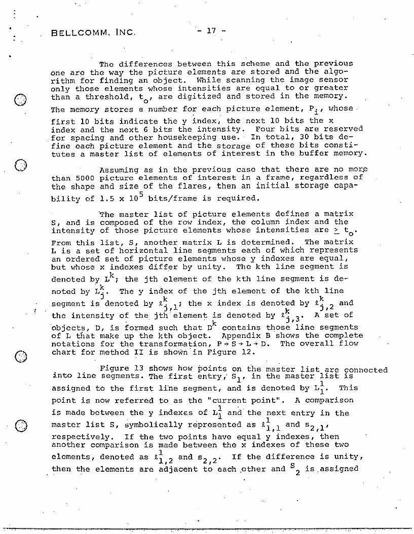
The differences between this scheme and the previous one are the way the picture elements are stored and the algorithm for finding an object. While scanning the image sensor only those elements whose intensities are equal to or greater

CZJ than a threshold, to' are digitized and stored in the memory.

0"', , '

The memory stores a number for each picture element, P., whose, . , ~

first 10 bits indicate the y index, the next 10 bits the x index and the next 6 bits the intensity. Four bits are reserved

,for spacing and other housekeeping use.' In total, 30 bits define each picture element and the storage of these bits constitutes a master list of elements of interest in the buffer memory.

Assuming as in the previous case that there are no mor~ than 5000 picture elements of interest in a frame, regardless of the shape and size of the flares, then an initial storage capa-

bility of 1.5 x 105 bits/frame is r~quired.

'The master list of picture elements defines a matrix S, and is composed of the row index, the column index and the intensity of those picture elements whose intensities are> t .

- 0 From this list, S, another matrix L is determined. The matrix L is a set of horizontal line segments each of which represents an ordered set of picture elements whose y indexes are equal, but whose x indexes differ by unity. The kth line segment is

denoted by Lk i the jth e'lement of the kth line segment is de

noted by L~. The y index of the jth element of the kth line

segment isJdenoted by £~,li the x index is denoted by £~,2 and

the intensity o~ the, jth'elemen~ is denot~d by £~,3. A set of

'objects, 0, is formed such that ok contains those line segments of L that make up the kth object. Appendix B shows the complete notations for the transformation, P ~ S ~ L ~ o. The overall flow

C;) chart for method II is shown'in Figure 12.

0"'" . ,

: i', ~.r

Figure 13 shows how points on ihe master list are connected into line segments. The first entry,' Sl' in the master list is

1 assigned to the first line segment, and is denoted by Ll • This

point is now referred to as the "current point". A comparison

is made between the y indeXeS of Li and' the next entry in the

master list S, symbolically represented as £i,l and s2,1'

respectively. If the two points have equal y indexes, then another comparison is made between the x indexes of these two

1 elements, denoted as £1,2 and s2,2. If the difference is unity,

then the elements are adjacent to each .other and S2 is .assigned

, .

•

,

(7) V

Q, " '~,

• :'1'


to Ll and this becomes the new current point, L~. A new line

segment is initiated tally adjacent to the until all elements of ments.

whenever the next point is not horizoncurrent point. Th~ procedure is continued S are redefined in terms of the line seg-

The next' process is to define objects, composed of the previously defined line segments. The general procedure is shown in Figure 14(a) and 14(b) ~ .and the detailed one in, Figure 15. The main idea is ,to ,find a connected set ,of line segments. The line segment which is compared, against the next segment in the list is called the "current line,"* denoted by

D~. Initially the first line of the L list is assigned as the

"current line".

There could exist three situations while comparing the y index of the current line and that of the next line in the list; 1) the difference is zero, which means 'that the two line seg~ents are in the same row; 2) the difference is unity, which means that the two lines are in adjacent rows and there exists a possibility of connection between them; and 3) the difference is more than unity, in which case, there is no possibility of the present line or any others further, down on list L belonging to the current object, and the process is repeated for a new object.

In the first case, when the y indexes are equal, an index 'Y' is incremented and this keeps incrementing until the y indexes of the current line and a subsequent line in the master ,list differ by unity. The number 'y' indicates that there are Y line segments to the right of and on the same y as the current line. This number is retained so that when there exists a next current line, which must be below the 'y' line segments,' a search is conducted for a possible connection between that current line and line segments corresponding to the number Y.

In the second case, when a unit difference exists between the y index of two lines, the ne.xt step is to find

whether any portion of o~e line (Li) is directly under the

other (D~). The test is performed by taking the difference J

of the x indexes of the first points of the two lines. This

d 'ff nk nl. 'd d b lid" 'd ld l. erence, j,2 - hl,2' l.S enote y . Agal.n, wou

have one of three values: 1) d=O, 2) d<O, or 3) d>O.

*From here on IIline ll and 1I1ine segment ll will be used interchangeably.

•

r>. ~jI

0,··,' ...

',' "

BELLCOMM. INC. - 19 -I I

For d=O, the first point of'Li lies directly'under

the first point' of the line D~, the current line. This indi

cates that the line Li belongs to the object Dk. The line Li is k now assigned as the new current line, D., and the entire process J

is repeated for the next line in the master list L.

k For d<O, and also if Idl is < n(D.), the number of

elements in the current line D~, then ~ poriion of the line Li

lies under D~. Hence Li belon~s to the kth object and is

assigned as fhe new current 'line. ' If Idl is > n(D~)' then no

part of Li is directly or diagonally under D~. This situation . J

indicates that the line L1 lies entirely'to the right of the

current line D~, and, therefore, the lines further right than . J ' k '

L1 and whose y's are the same as Dj would not have any connec-

ti vi ty wi th D~'.

i If d>O,and the value of Idl is < n(L) the number of

elements of line Li , 'then some portion of Li is directly or diagonal~y under the current line, and, therefore, the line

segment Li belongs to the current object. The line Li is now

assigned as the new "currerit line", D~. In case Idl > n(Li ),

th l · i h ... h J k ' . d d d b e 1ne L as no connect1v1ty W1t D., an 1n ex enote y J .

'a' is incremented and the process is repeated for the next line segment. It is necessary to keep information (the index a) on

the lines which do not show any connectivity with D~ so that J '

they can be checked later to find connectivity with future current lines.

After the next current line is found, the value of 'a' is transferred to a temporary storage register E but only if this register is empty. The purpose of this step is to allow a to be reset to zero before the next row is processed. If E is not empty, it means that the previous current line had lines horizontally adjacent to its left, i.e., above and to the left of 'the current line. These lines are then checked for connectivity with the current line. They are marked and placed on the secondary list if they ar~ connected.. After all lines corresponding to the contents of E have been checked, the current value of a is transferred to E.

, . ' 4 '>, p '., , .. ' /' ~

".

•

o

0" , .

;j,

BELLCOMM, INC. - 20 -

Next, the value of Y is checked and if y > 0, then there are lines above and to the right of the current line. They a're then checked with the current line for connectivity, and are marked'and placed on the secondary list if they are connected. The above process can be clarified by referring to the example in Appendix c.

By the above procedures, some of the lines are assigned outright to the current object and some are placed on a secondary list as po'tentia1 starting points for additional

'branches of the object. Once the difference of y indexes between the current line and the next line is more than unity, the program jumps to pick up marked lines from the secondary list. The first marked line in the secondary list is assigned as the current line. A test is performed to find if there is any other unassigned line in the master list of line segments that lie above or below the current line. In the latter case, the program follows the same procedure described above; but in the forme~ case, the program has to move upwards over the master list. The right hand portion of the flow chart, Figure 15, shows the procedure. The difference for upward movement is that "a" represents the lines to the right of the current line and "y" represents the lines to the left. Since the program is moving upwards in the list, the line index will be decreasing, i.e.,' i= (i-1) in each step, and when i= Ois reached, tile program again goes over to the secondary list and picks up another current line, provided that the line was not assigned in the previous process.

'When the secondary list has no more marked lines, the program has defined the current object. The total number of elements contained in the object is the summation 'of the number ,of elements in the lines belonging to the' object, and this also gives the area of the object. The area thus obtained is the observed or the apparent area of the object, and needs correc.tion for the geometric forE?shortening.

Once all objects of the fram~"are defined, the next

step is to compute their centroids (:X ~ y 1. The flow chart to implement this is shown in Figure 16. Once the centroid is known, the distance 'r' between the center of the Sun and the centroid of the object can be determined by simple calculations. Then, the corrected area "of the object, can be computed by the use of a formula such as that given on page 6. The next step is to determine'the maximum arid average intensities of each object in the frame. These two parameters are determined by the procedure shown in Figure 17.

',~ ,';:',~, ,

:' ~ ":' /, .

! r '~' ":'; ,. ", . ~ , ," I

•

-..

O~, , ,

- 21 -

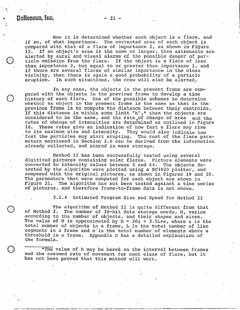
Now it is determined whether each object is a flare, and if 'so, of what importance. The corrected area of each object is compared with that of a flare of importance 2, as shown in Figure, 12. If an object's area is the same or la~ger, then astronauts are alerted by aural and visual alarms of the possible danger of particle emission from the flare. If the object is a flare of less than importance 2, but equal to or greater than importance 1, and if there are several flares of similar importance in the close vicinity, then there is again a good probability of a particle eruption. In such situations, the drew will also be alerte~.

In any case, the objects in the present frame are compared with the objects in the previous frame to develop a time history of each flare. One of the possible schemes to determine whether an object in the present frame is the same as that in the previous frame is to compute the distance betvleen their centroids. If this distance is within some limit "h",* then the objects are considered to be the same, and the rate~of change of area and the rates of change of intensities are determined as outlined in Figure 18. These rates give an indication of how fast a flare may rise to its maximum size and intensity. They would also indicate how

'fast the particles may start erupting. The rest of the flare parameters mentioned in Section 2.6 can be derived from the information already collected, and stored in mass storage.

Method II has been successfully tested using several digitized pictures containing solar flares. Picture elements were converted to intensity values between 0 and 64. The objects detected by the algorithm were plotted us~ng a SC4020 plotter, and compared with the original pictures, as shown in Figures 19 and,20. The parameters that were computed for each object are shown in Figure 21,. The algorithm has not been tested against a time series of pictures, and therefore frame-to-frame data is not shown.

3.2.4 Estimated Program Size and Speed for Method II

The algorithm of Method II is quite diffe~ent from that of Method I'. The number of 30-bi t data storage words, M, varies according to the number of objects, and their shapes and sizes. The value of M ~s approximated by M = 20~ + 3.5L+e, where ~ is the total number of objects in a frame, L is ,the total number of line segments in a frame and e'is the total number of elements above a threshold in a frame. Appendix D has a detailed explanation of the formula.'

*The value of h may be based on the interval between frames and the assumed rate of movement for each class of flare, but it has not been proved that this method will work.

o

0_', ',," ~ ,J'

. '

Bellcomm, Inc. 22

/

Figure 22 shows plots of the number of flares/frame against M. For 90mputation purposes, it, is assumed that a f~are has a square or rectangular configuration, and its overall area- is taken as an upper bound of 'a flare importance range given in Table'l. The plots of Figure 22 show ~emory data storage requirements for flares of importance I , 1,2,3, and 4. If a data storage estimate is desired for a variety of flares occurring simultaneously, then the number of data \vords can be approximated by adding the values of M obtained separately from Figure 22 for each importance class. Considering the same example as in Method I (one flare of importance 4, one of importance 2, two of importance 1, and five subflares), the number of data storage words required is 5786 (M=2733+l066+942+1045).

, Based on actual coding of Method II in Fortran V on a Univac 1108, the overall instructions should require <, 2000 woras. Thus, in the above example, the total memory requirement is < 7.8 X 10 3 , 30-bit words.

In order to show the effect of flare shapes on the data storage, Appendix D contains two formulas, one for elongation of a rectangular flare along the y direction and the other in the x direction. Table 4 contains correction factors based on these formulas for a single flare per frame. A correction for multiple flares can be obtained by.multiplying the correction factors of Table 4 by the number of flares in a frame. In general,

a memory of 1 x 10 4 , 30-bit words capacity is sufficient and can handle most likely combinat~ons of flares occurring silnultaneously.

The number of operations/sec. required to process a complete frame also depends on the size, the number and the shape of the objects. A conservative estimate can be made by again considering the example in Hethod 1. It is conservatively as-sumed that On an average each line segment is 5 elements long. Hence, the total number of lines in the example frame would be 1000.

e) Since this method works from the list of points in a _ frame, the first job for the computer is to connect the points . into line segments. This is a simple operation of comparison of the x and y' coordinates of each point and would not take more than 45 operations/point on an average. The next operation is to connect the set of line' segments into objects. This is the most complicated step and is a function of the size, shape, and number of objects in the frame. 'A conservative estimate is an CD average of 600 operations/line segment.* Once an object has

*All speed estimates here are based on the program written in Fortran V without special attention to making it run fast. On a modern spaceborne computer with an' ove-r 50 :,instruction reperto.ire, the program could be written to use less operations. '

n v

0, . ' ,

BELLCOMM, INC. 23 -

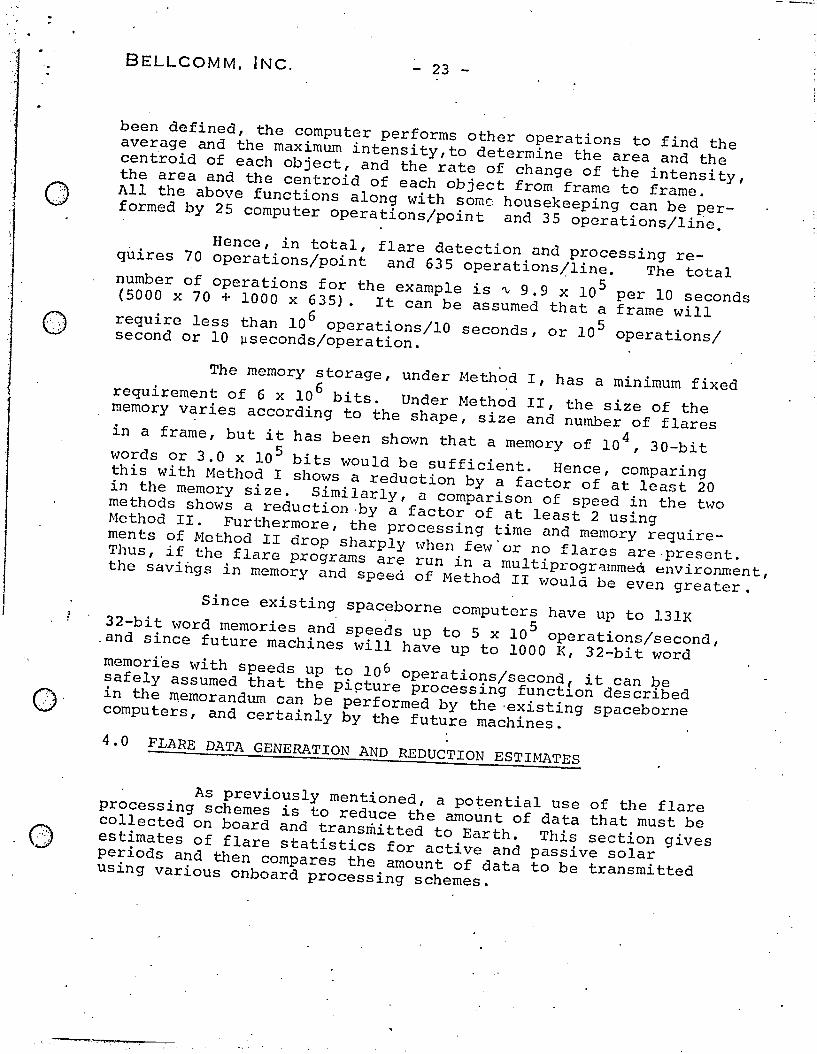
been defined, the computer performs other operations to find the average and the maximum intensity,to determine the area and the cent'roid of each object, and the rate of change of the intensity, the area and the centroid of each object from frame to frame. All the above functions along with some housekeeping can be performed by 25 computer operations/point and 35 operations/line.

Hence, in total, flare detection and processing requires 70 operations/point and 635 operations/line. The total number of operations for the example is ~ 9.9 x 105 per 10 seconds (5000 x 70 + 1000 x 635). It can be assumed that a frame will require less than 10 6 operations/IO seconds, or 105 operations/ second or 10 ~seconds/operation.

The memory storage, under Method I, has a minimum fixed requirement of 6 x 10 6 bits. Under Method II, the size of the memory varies according to the shape, size and number of flares in a frame, but it has been shown that a memory of 10 4

, 3D-bit words or 3.0 x 105 bits would be sufficient. Hence, comparing this with Method I shows a reduction by a factor of at least 20 in the memory size. Similarly, a comparison of speed in the blO methods shows a reduction ,by a factor of at least 2 using Method II. Furthermore, the processing time and memory requirements of Method II drop sharply when few'or no flares are ,present. Thus, if the flare programs are run in a multiprogr"lmmeci environment, the savings in memory and speed of Method II would be even greater.

Since existing spaceborne computers have up to l31K 32-bit word memories an~ spee~s up to 5 x 105 operations/second, ,and since future machines will have up to 1000 K, 32-bit word memori~s with speeds up to 10 6 operations/second, it can be safely assumed that the pi~ture processing functlon described in the memorandum can be performed by the 'existing spaceborne computers, and certainly by the future machines .

4.0 FLARE DATA GENERATION AND REDUCTION ESTIMATES

As previously mentioned, a potential use of the flare processing schemes is to reduce the amount of data that must be collected on board and transmitted to Earth. This section gives estimates of flare statistics for active and passive solar periods and then compares the amount of data to be transmitted using various onboard processing schemes.

0', , "

, '

o

/2:t V

BELLCOMM. INC. 24

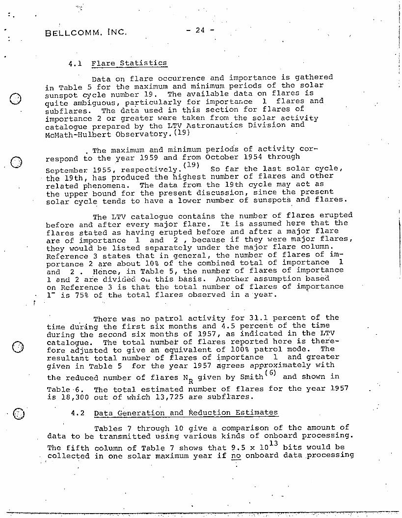
4.1 Flare Statistics

Data on flare occurrence and importance is gathered in Table 5 for the maximum and minimum periods of the solar sunspot cycle number 19. The available data on flares is qui te ambiguous, pa;r-ticularly for importar!ce 1 flares and subflares. The data used in this section for flares of importance 2 or greater were taken from the solar activity catalogue prepared by the LTV Astronautics Division and McMath-Hulbert Observatory~ (19) ,

. The maximum and minimum periods of activity correspond to the year 1959 and from October 1954 through

September 1955,' respectively'. (19) So far the last solar cycle, the 19th, has produced the highest number of flares and other related phenomena. The data ,from the 19th cycle may act as the upper bound for the present discussion, since the present solar cycl~ tends to have a lower number of sunspots and flares.

The LTV catalogue contains the number of flares erupted before and after every major flare. It is assumed here that the flares stated as having erupted before and after a major flare are of importance 1 and 2, because if they were major flares, they would be listed separately under the major flare column. Reference 3 states that in general, the number of flares of importance 2 are about 10% of the combined to'ta1 of importance 1 and 2. Hence, in Table 5, the number of flares of importance 1 and 2 are divic:iea Ou this basis. Another assumption based on Reference 3 is that the total number of flares of importance 1- is 7S% of the total flares observed in a year. '

. There was no patrol activity for 31.1 percent of the time during the first six months and 4.5 percerit of the time during the second six months of 1957, as indicated in the LTV catalogue. The total number of flares reported here is ther'efore adjusted to give an equivalent of 100% patrol mode. The resultant total number of flares of ~mportance 1 and greater given in Table 5 for the year 1957 agrees approximately with

the reduced number of flares NR given by Smith(6) and shown in

Table 'G. The total estimated number of flares for the year 1957 is 18,300 out of which 13,725 are subfl'ares.

4.2 Data Generation and Reduction Estimates

Tables 7 through 10 give a comparison of the amount of data to be transmitted using various kinds of onboard processing.

The fifth column of Table 7 shows that 9.5 x 1013 bits would be collected in one solar maximum year if ~ onboard data ,processing

. -.

0), V

o

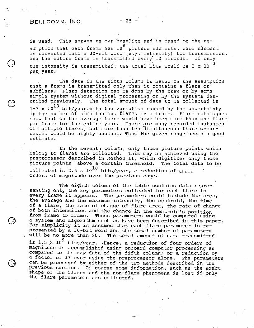
BELLCOMM, INC. - 25 -

is used. This serves as our baseline and is based on the as

sumption that each 'frame has 10 6 picture elements, each element is converted into a 3D-bit word (x,y, intensity) for transmission, and the entire frame is transmitted everi 10 seconds. If only

. 13 the intensity is transmitted, the total bits would be 2 x 10 per. year.

The data in the sixth column is based on the assumption that a frame is transmitted only when it contains a flare or subflare. Flare detection can be done by the crew or by some simple system without digital processing or by the systems described previously. The total amount of data to be collected is

1-7 x 1013 bit/year,with the variation caused by the uncertainty in the number of simultaneous flares in a frame. Flare catalogues show that.on the average there would have been more than one flare per frame for the entire year. There are many recorded instances of multiple flares, but more than ten iimultaneous· flare occurrences would be highly unusual. Thus the given range seems a good estimate.

In the seventh column, only those picture points which belong to flares are collected. This may be achieved using the preprocessor described in Method II, which digitizes only those picture points above a certain threshold. The total data to be

collected is 2.6 x 1010 bits/year, a reduction of three orders of magnitude over the previous ca~e.

The eighth column of the ~able contains data representing only the key parameters collected for each flare in every frame it appears. The parameters could include the area, the average and the maximum intensity, the centroid, the time of a flare, the rate of charige of flare area, the rate of change of both intensities and the change in the centroid's position from frame to frame. These parameters would be computed using a system and algorithm such as have been described.in this paper. For simplicity it is assumed that each flare parameter is represented by a 3D-bit word and the total number of parameters will be no more than 20. The total amount of data transmitted

is 1.5.x 109

bits/year. ·Hence, a.reducf~on of four orders of magnitude is accomplished using onboard computer processing as compared to the raw data of the fifth column; or a reduction by a factor of 17 over using the preprocessor alone. The parameters can be processed by either of the two methods described in the previous section. Of course some information, such as the exact shape of the flares and the non-flare phenomena is lost if only the flare parameters are collected.

. ' ",

Q" ~, " ,

0,,' "

0', " ,

Belh::omm,! Inc. - 26 -;

If flare shapes are desired then an additional amount of data is required. Using the first method, described in Section 3.0, the boundary points of a flare along with the data on the flare parameters of the eighth column are collected.

This combined data is 5.9 x 10 9 bits/year, given in the ninth column. This shows a reduction by four orders of magnitude compared to the raw data. . ,

Using the second method, only the first point and length of each line segment belonging to a flare are collected in order to reconstruct the flare shape. The total data col-

lected in this case i~ 3.8 x 10 9 '- 1.2 x 1010 bits/year as given in'the last column of Table 6. The lower range is based on square flare configurations while the upper is based on t'he previous assumption of five elements to.a line segment. These two assumptions give a different number of line segments in a frame. This still shows a reduction by three to four orders of magnitude compared to the raw data.

A similar analysis is given in Tables 8 and 9 for the most active month and day of the solar cycle number nineteen. Column seven of these tables again shows a reduction of four orders of magnitude compared to the' raw data of column five. The data reduction is of the same order of magnitude for the most active day, month and year of the solar cycle.

Table 10 indicates'the amount of data that can be generated during the minimum phase of the 'solar cycle. It is assumed here that there are no multiple occurrences of flares, that is, a single flare per frame. A reduction of six orders, bf magnitude is indicated when the data of the seventh column where only flare parameters are collected, is compared with the raw data shown in the fifth column.

5.0 APPLICATION OF THE SYSTEM TO OTHER PHENOMENA OF THE SUN

A similar scheme to the one described for flare detection could be applied to detect and observe plages. It could be done either by interrupting flare processing every 10 minutes, automa~ically changing the 'Ha filter to the CaII-K filter, and

".

processing plages for 10 seconds, (one frame time); or by using separate plage and flare sensors within a multi-barrel telescope.

<=) The importance of plage observations can b~ broken down into two categories: '(1) scientific study of the plages phenomenon itself, and (2) correlation between plages and flare eruption. The area, brightness and luminosity changes of a calcium plage region are the basis for flar,e prediction in the presence of bipolar or , more complex magnetic regions. A statistical method based on these

!

BELLCOMM. INC, ~ 27

parameters has been developed by which large flares can be pre

dicted from 21 to 35 days in advance. (20) The chromospheric brightening in CaII-K' line is also a stable optical indication (J) of the formation of an active region.

0", " :

During 1957-69, out·of 984 flares, 75% of 'the flares were associated with regions that had at least one previous disk passage. Flares associated with a newly formed p1age ,region can be predicted from the behavio'r of the magnetically active regions, which are observable before the appearance of p1ages.

Another phenomenon of interest, which has a correlation with solar flares is sunspots. Observations of sunspots can also be conducted by the solid state image sensor. Since the sunspots does not change in intensity and shape as violently as flares do, it is possible to read the sunspots data every 5 to 10 minutes and process the information in a single frame time. Again, sunspot detection can be integrated into the flare detection system just as p1age detection mentioned earlier; or a separate sensor can be used with its own small processor. The correlation of flares with sunspots and p1ages may permit good flare prediction.

6.0 SUMMARY AND CONCLUSIONS

A spaceborne system has been proposed that will automatica11y'detect solar"flares. The system contains a telescope equipped with monochromatic filters, a solid state imaging ,tube, and an onboard digital computer. ,The solid state sensor contains

10 6 photodiodes in an area array and is scanned by an electron beam as is done in a vidicon .. The output'of the image sensor after oig1tizing is fed 1nto an onboard digital computer for extracting flare information such as the area, the maximum and average intensities and the rate of change of the area and the intensities. The proposed 'system can also detect other phenomenona of the Sun such as sunspots and pl~ges.

Two different methods have'been shown for processing flare information. ' In the first method, a search for a boundary point of a flare is conducted. Once a point over an intensity threshold is located (a boundary point) the onboard processor defines the boundary of the flare. Then the area and maximum and average intemsi ties are ca,lculated.

In the second method, the processing is performed on a selected list of points which are over an intensity threshold. These points are connected into horizontal line segments and then the line segments are connected to define flares.

· . '.

o


The memory requirement for the first method is

> 6 x 10 6 bits whiie for the second method it will not exceed

3 x 10 5 bits. The number of operations required to process a

frame in the first method is > 2 x 10 5 operations/second and

for the second method the number is < 10 5 operations/second. Thus, automated flare detection is a feasible function for. spaceborne computers to perform, and crew man-hours may be saved.

It has also been shown that tremendous data reduction ratios are possible using preprocessing and computer analysis of solar images. The reduction can be as much as three to four orders of magnitude in the active year and six orders of magnitude in the passive years of a solar cycle.

Tbere are many problems relating to flare detection that have not been discussed. For example, the detection algorithms can furnish enough information to discriminate flares from noise, but experimentation with actual hardware and more flare data is needed to prove this. There are other techniques, such as averaging two frames, that may be more efficient as noise suppressors if noise turns out to be bothersome;

Another untreated problem is the motion of the sun's image on the sensor. There would be sufficient information to determine the position of a flare relative to the sun rather than the sensor, but again the details'have not been worked out in this study.

, Nevertheless, the study has demonstrated the general feasibility of the approach and the potential for reducing crew time, data storage, and data transmission requirements. This should provide. the incentive to further examine solar flare

~ detection and other experiments for their potential use of V spaceborne computers.

7.0 ACKNOWLEDGEMENT

The author wishes to th,ank Mes·srs. D. O. Baechler, A. N. DeGaston, R. H. Hilberg, J. J. Rocchio, P. S. Schaenman, and D. B. Wood of Bellcomm, Inc.; Mr. P. Higgins of MSCi and Dr. H. Glaser of NASA Headquarters, for many helpful discussions; Mr. R. R. Singers of Bellcomm, Inc., for ,analysis, programming and simulation of flare processing using Method IIi and Mr. P. E. Tallent of Sacramento Peak Observatory, Air Force Cambridge Research Laboratories, Sunspot, New Mexico for an

, ,

· !

0'" , I."

r:'\ ~

()

r':\ V

"BELLCOMM, INC. - 29 -" ,

interesting discussion and for providing the photographs of the Sun used in this memorandum.

l031~RKA-szm

Q k· [~\i1I'P )1.v{l,~i R. 'K.- AgaVwal ,

Attachments

"

".

BELLCOMM. INC.

REFERENCES

@ 1." A Solar Flare' Videometer," Paul E. Tallent, Sacramento Peak Observatory, U. S. Air Force Service (l1AC) USAF, July 1967.

o

o

2. "A Solar Flare Measuring System Using Video Techniques," Olin L.Graham, National Telemetering Conference, p. 169, April 1968.

3. IIHandbook of Geophysics and Space Environrnents," Edited by Shea L. Val~ey, McGraw Hill, 1965.

4. "The Sun," G. Abetti, 1962 Edition, Faber and Faber.

5. "The P'hysics of Solar Flares," AAS-NASA Symposium, SP-50, Goddard Space Flight Center, October 28, 1963.

6. "Solar Flares," Henry J. Smith and Elska V.P. Smith, MacMillian Company, 1963.

7. "Geophysics and Space Data Bulletin," Volume II-No.1, First Quarter, 1965.

8. "statistical Evaluation of Proton Radiation From Solar Flares," Final Tech. Report, JPL Contract 951293, North American Aviation Inc., 29 July 1966.

9." "Solid State Imaging," Special Issue, "IEEE Transaction on El~ctron Devices, Vol. ED-IS, No.4, April 1968~

10. "A Camera Tube with a Silicon Dio~e Array Target," M. H. Crowell, T. M. Buck, E. F. Labuda, J. V. Dalton and E. J. Walsh, The Bell System Technical Journal, Vol. 4, p. 491, February 1967.

11. "An Electron Beam-Accessed Image-Sensing Silicon-Diode Array with Visible Response," M. H. Crowell, T. M. Buck, E. F. Labuda, J. V. Dalton and E. J. Walsh - International Solid State Circuit Conference, p." '128, February 1967.

12. "The Silicon Diode Array Camera Tube," M. H. Crowell, E. J. Labuda, The Bell System Technical Journal, MayJune 1969.

! . , . • BELLCOMM. INC .

I I

BIBLIOGRAPHY

This bibliography cites significant documents which have been consulted in the preparation of this memorandum. Each of the following parts corresponds to a particular section in the report.

Solar Physics - Flares, Plages, and Sunspots

"Astrophysical Quantities," C.W. Allen, University of London Press.

~I Solar System Astrophysics," Brandt and Hodge, (McGraw-Hill).

liThe Solar Spectrum," Astrophysics and Space Science Library, edited by C. deJager, D. Reidel Publishing Company.

I

"Tlw Solar System, If Astrophysics III, Handback Der Physik, Vol. LII.

"statistical Evaluation of Proton Radiation from Solar Flares," Final Tech Report, JPL Contract '951293, North American Aviation, Inc., July 29,1966 ..

"Significant Achievements in Solar Physics, 1958-64," NASA-SP-IOO.

"Interplanetary Craft for Advanced Research in in the Vicinity of the Sun," (ICARUS), N67':"14203, Aug. 1966.

"Preliminarv Study of Prediction Aspects of Solar Cosmic Ray Events," K. A,. Anderson, NASA TND-700, ,April 1961.

"Solar Longitude Distributions of Proto~ Flares, Meter Bursts, and Sunspots," Marion W. Haurwitz Inst. of Teleconununication Science and Aeronomy, ESS Administration, Boulder, Colorado.

"A Daily Index of Solar Flare Activity," Constance B. Sawer, J. of Geophysical R~search, Vol. 72, No.1, p. 385, Jan. 1, 1967.

-.

"Thermal Instabilities in the Solar Chromosphere," James H. Hunter, Jr., ICARUS 5, p. 321, 1966.

"Scientific Considerations of an Early Dccoupled ATM Mission at an Inclination of 50°," Case 630, D. B'. Wood, Bellcomm Memorandum. for File, June 5, 1968" '." . ," . .

"Variations of Interplanetary Solar Cosmic Ray Radiation Hazard with Solar Cycle," A. N. CleGaston, Bel~comm Memorandum for File, October 25, 1966 •

. ."

o

0, :,,'

o

0' " ". -. ';".

BeUcomm, Inc. - 2 -

"Flare Prediction from Solar Limb Obser'vations," Lorne Avery and Donald E. Billings, Astro-Geophysical Memorandum No. 163 May 5, 1964, High Altitude Observatory, Boulder, Colorado.

"Basic Solar Research," o. C. Mohler, Michigan University, October 1965, N66-l9427.

"Joint Discussion ot' Solar Flar,es," Transactions of International Astronomical Union, Vol. 648, p. 648, 1957.

"Sol~r syste~ Radio Astronomy," Lectures Presented at the NATO Advanced Study Institute of the National Observatory of Athens, Cape Sounion, Greece, 1964. Edited by Jules Aarons, (Plenum Press) •

"Optical Characteristics of Cosmic Ray and Proton Flares," Anton Bruzek, Journal of Geophysical Research, Vol. 69, No. 11, p. 2386, June 1, 1964.

"Theory of X-Ray Emission of the Sun" - G. Elwert, Journal of Geophysical Research, Vol. 66, No.3, p. 391, February 1961.

"Solar Interplanetary Study," Final Report, NASA-N67-37283, August 1967.

"Geophysical and Space Bulletin," Vol. II, No.1, 1st Quarter 65, AD62l3l4.

"System for Solar Flare Prediction," D.E. Billing, Colorado University, Boulder, June 1965, N66-l~673.

~High-Resolution Photography of the Solar Chromosphere III: The Fine Structure of a Class I ~lare," R • .E. Loughhead, Solar Physics, Vol. 4, No.4, p. 422, August 1968.

'Solid State Sensors and Their Applications

"A Charge-Storage Diode Vidicon Camera Tube," P. H. Wendland, IEEE Trans. on Electron Devices, Vol. Ed-14, No.6, p. 285. June 1967.

"A Possible Electron Image Information Store," A. D. Berg and.R. W. Smith, Imperial College of Science and Technology, London, N67-l3066.

"Charge Storage ),ights the Way ,for Solid State Image Sensors," Gene P. Weckler, Electronics, p. 75, May 1, 1967.

"New Dimensions for Interferometer," R. E. Brooks, Electronics, 88, May 1, 1967.

'.! ~,) ,Pi , -, ", ,.' F

A V

0, "

o V

. BeUcomm, Inc. 3 -

"Image Converter Camera for 0.5 to 10,000 Microsecond Photographs" - H. L. Miller, Plasma Physics Laboratory, Princeton University, N. Y., American Inst. of Aeronautics and Astronautics.'

"A Daylight Astro Tracker for Supersonic Transport Navigation," Joel Greene, J. of the Inst. of Navigation, Vol. II, No.3, p. 228, Autumn 1964.

"Photoelectric Telescope Observations," U. G. Fresenkov, 1965, N66-l775l.

"Resolution criteria for Optical and Photographic System," F. Oharek, Naval Training Device Center, Florida, October 1967, AD-660680.

"Remote Sensing of Natural Resources," by Robert N. Colwell. Scientific American, p. 54, January 1968.

"A Precision' Flying Spot Film Digitizer ,"71 Jerome A. 'G. Russell, December 1963, N64-l729l.

'"Optical Spot Size Study for Data Extracticin from a Trans, parency, " L. L. Izzo, et al., September 1965, AD-:-628588.

- "Scanner to Examine Chromosome Changes,1I Roderick D. Hibben, Aviation Week and Space Technology, p. 95, December 6, 1966.

liThe Surveyor Lunar Landing Television Systems,lI Donald R. Montgomery, IEEE Spectrum, p. 54, August, 1966.

Picture Proce3sing and Pattern Recogriition

"Pictorial Pattern Recognition," edited by George C. Cheng, 1968 (Thompson).

"Picture Processing by Computer,1I Azrie1 Rosenfeld, Computer Science Center, University of Maryland, Technical Report No. 68-71, June 1968.

"A Transformatio!l for Extracting New Descriptors of Shape," Harry Blum, Symposium Proceeding, Models :eor the Perception of Speech and Visual Form,' edited by Wei~nt Wathem-Dunn, p. 362, November 11, 1964 •

. 0 "A Survey of Pictorial Data Processing Techniques and Equipments,1I Andrias Van Dam, August 1965, AD-626155.

"Research of the utilization of Pattern Recognition Techniques to Identify and Classify Objects in Video Data," Tech. Progress Report No.2, October 1965 through May·1996, Douglas Aircraft, N66-39924. '

".

I

0:· ..

0'· .. .,.11"

0" ,", • ,;,,>

- 4 -

. I

"A Digital/Approach to Photographic Image Quality Evaluation," Gene A. Markel, e~ al., HRB-Surveyor, May 1967, AD-653084.

"A Study of Discrete p~ogation-~ased Models for Pictorial . Pattern Analysis," A. Rosenfeld, J. L. Pfaltz and H. Kafafean, Final Report, June 1967, AD-659l58.

"Sequential Operations in Digital Picture Processing," Azriel Rosenfeld and John L. Pfaltz, J. of ACM, Vol. 13, No.4, pp. 471-494, October 1966.

"Labeling Schematic and Syntactic Descriptions of Pictures," R. Varasinham, Information and Control, Vol. 7, pp. 151-179, 1964 •

"An Adaptive Pattern Recognition Machine Using Bi-Polar Threshold Logic Devices," W. C. Lin and K. S. Fu, Purdue University, Proc. Nat. Ele. Conf., pp. 535-540, 65,.

"Visual Pattern Recognition by Moment Invariants," Ming-Kuei Hu, IEEE Trans. on Information Theory, p. 179, February 1962.

"Automatic Target Recognition: Some Considerations," S. F. Smillie, IEEE Transection of ~erospace and Electronic Systems, Vol. AES-2, No.2, p. 187,- March 1966.

. . "In-Flight Decision Systems,lI Final Report, The Bendix Corp., February 1966, AD-477959.

"An Abstract Model for the Pattern Recognition Process,1I Ceroley Electronic Laboratory, April 196 , AD-6l2037.

IIPattern Recognition,' Functionals and Entropy,~ H. J. Bremermann, August 1967, AD-659197. .

"A System of Pattern Recognition Independent of Displacement Scale and Orientation," A. K. Edger, November 1966, N-67-38443.

IIDevelopments of Machine Translation and Information Processing (No. 132)," Translation from Russian Language, 'September 1964, TT-G3-31172.

"A Model for the Random Vide'o Process," L. E. Franks, The Bell System Technical Journal, p. 609, April 1966.

IIPattern Recognition by Linear Programming," Malcolm· S. Taylor, July 1967, AD~656928.

, i" t •

-.

"",

o

o

J

- 5 -

Data Gathering and Processing

"Optimization of Instrumentation of Space Experiments from the Standpoint of Data Processing-Part III," Space Research VI, Proc. of the Sixth International Space Science Symposium, edited by R. L. Smith, (MacMillan & Company), Mar Del Plata, Argentina, May 11-19, 1965. .

The following three papers are most pertinent to this study:

"Processing of Telemetering Data Generated by Sensors Moving in a Varying Field," D. J. Pakinson, Dept. of Electrical Engineering, University of California, Berkeley, California.

"On-Board Data Processing in Spacecraft as an Aid to Optimizing the Design of Experiment," A. P. Willmore, Phy. Dept. University Coll~ge, London.

"Parallel Decoding and Optimization of Data P~ucesslng of Space Experiments," B. S. Fleisman, Academy of Science, Moscow, USSR.

,

0,;': ''''(

"

o

o

0:',: ,,'

,'; ; ,J '. f " .. ,

~Ependix A

Image Sensor's Resolution

Sensor dimensions = l"xl" (Optic:'lal)

Density of the sensor = 106 diodes (or picture elements)! . 2 l.n •

Solar Diameter = 1.38 x 106 km.

Chromospheric thickness ~ 10 4 km.

Solar apparent diameter'~ 1.39 x 106 krn. , (used in all calculations in the memorandum)

Considering that the image of~the sun is focused on a square array, the sensor's resolution =

= 1. 93xl06km2 / (1. 39X106)2

10 3 . ;' , picture element

or in terms of heliographic equatorial square degrees*

1 deg 2 ~ 77 picture elements.

*units of heliographic equatorial squa~e degrees:

2 8 2 -6 1 deg = l.48xlO km = 48.5xlO of the solar hemisphere.

! .. ~ I

·~---------- -

. #

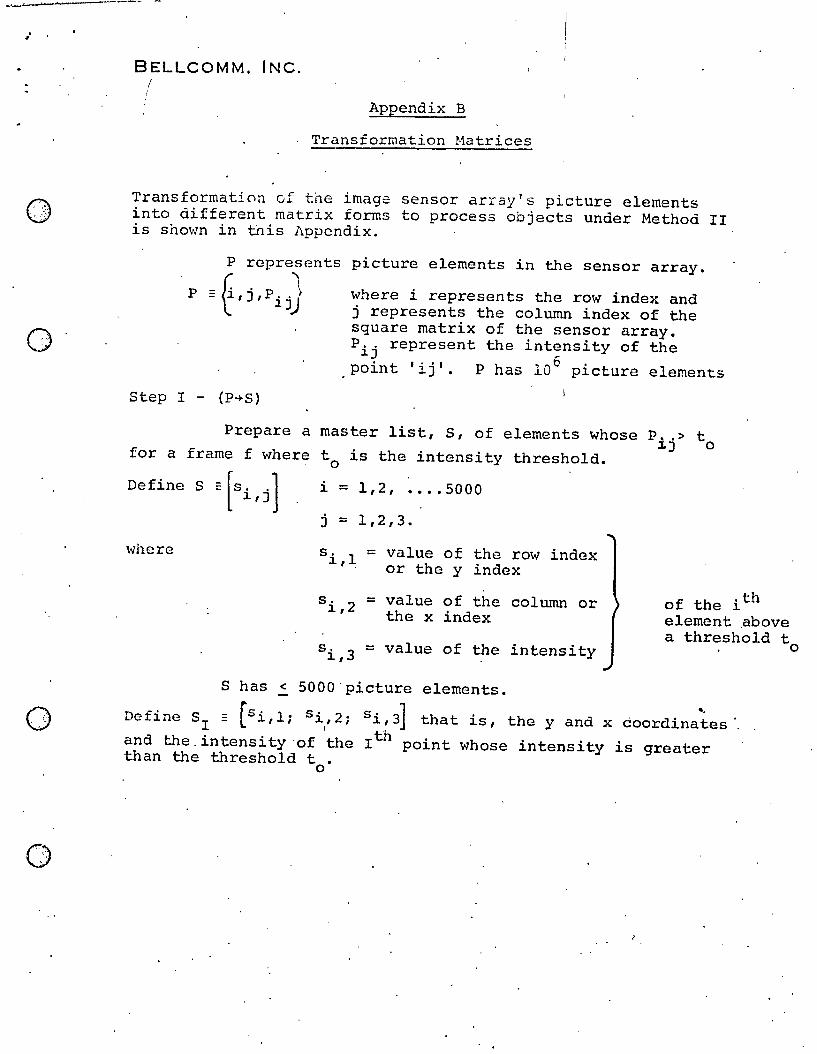
0 ', ' '.

o

o

BELLCOMM. INC. I

Appendix B

Transformation Matrices

Transformation of the image sensor array's picture elements into different matrix forms to process objects under Method II is shown in this Appendix.

P represents

- [;. ~ P = l",J,Pijj

picture elements in the sensor array.

where i represents the rot.; index and j represents the column index of the square matrix of the sensor array. P .. represent the intensity of the ~J '

point lijl. P has 10 0 picture elements

Step I - (P-+S)

Prepare a master list, S, of elements whose Pij > to

for a frame f where to is the intensity threshold.

Define S =[s .. J i = 1,2, •••• 5000 ~,J

j = 1,2,3.

' .... here s. 1 ~, ,

s. 2 ~,

s. 3 ~,

= value of the row index or the y index

= value of the column or the x index

= value of the intensity

S has < SOOO'picture elements.

of the ith element ,above a threshold t

D f · S [s. 1 s· 2 e ~ne I - ~,; ~/ ;

and the. intensity 'of the than the threshold t .

Si,3] that is, the y and x coordina~es·. Ith point whose intensity is greater

o

o

,

0,: 'e, i I,,'

0",'" .'

0 ,.',>

BELLCOMM. INC.

,Appendix B (Contd.) - .2

Step II (S+L)

L defines a set of

{L~. E L -

\lThere LK = r~j is

LK I - [ K 'i,l;

K ,. 1 = row index 1.,

K t. 2 - column index 1.,

"K = intensity i,3

horizontal line sogxr..ents.

{Ll, 2 m} L, ---L

the R t~l line' segment

t~ 1.,2; tt3 ] = Some SJ

'of the i th' point

in the K'th line

segment

The Kth line sigment, LK, will be made up of some set of consecuti,ve SI's, say (SI; SI+l; SI+2J where sI,l = SI+l!l 0 sI+2,1. However, the only'parameters that need to be stored are the x and y indexes of the 1st point in each line segment and the number of points in that segment.

Step III - (L+O)

L. D defines a set of objects made by linking members of '

Therefore 0 is defined as:

. 0 E~K) E (01 , 0 2 , ___ o"') . "There ol~.::, [d~.'. :] or oK = [o~]

. 1.J 1.J ,J

,where oj. = some LI = jth line segment in the }tth object.

' K index d. 1 = row 1., _

K d L2 " = column index of the i th point

K intensity in the Kth object dit3 " =

j q II .;: !)" , ~-

0" , , ~i.!

, ,

o

0<:: ','

Bellcomm, hee. l

Appendix C

I· I

Example of Connecting Line Segments to Form Objects Under Method II

The image processing scheme given under Method II can be clarified by the example shown in the figure at the end of the appendix. The number at the beginning of each line in the

figure indicates the "i" index of line segment Li. . 1 '

The first line segment L is assigned as a current

. line that belongs to the first object and is denoted by Di. A

comparison between D~,l and 1~,1 indic~tes the ~ifference'of unity. Nm'l, the different d between 01,2 and 1 1 ,2 1 is deter

mined. Referring to the accompanying table again, d = 0 which indicates line 2 is directly under the current line and belongs

to the current object. Now, the line L2 is assigned as the cur-l rent line D2 •

The y indices of D~ and L3 are the same. At this

stage, an index Iyl is increme~ted, and 1f, is checked against

the x index of the previous current line, D1~' The.value of 1 3 .

d = Dl ,2 - 11 ,2 = -8 and the value of n(D1) ~.7; therefore

Idl,> n(Dl ). Hence L3 is not designated as a member of the

first object, although it· may be by some later discovered con

nection. The program moves to test line L4, and a similar test

shows that it has no connection with the line Di. The 'y' is incremented again and now contains a n~ber 12 I.. Similar ".

tests on the next line, LS, show adjacency with current line

D~, hence, is belongs to the current object and is assigned as

the new current line D~.

At this point a check is made on the values E and y. The value of E is zero but the value of y ls g:r;eater than zero. The y represents lines to the right of the previous

current line D~, and has to be checked against the current line 1

D3 • The line corresponding to index 'b' of 'y' is given by .

i'+b il 1 L ,where L corresponds to the previous current line D. 1"

J-

; . , . ; ~" ~ : 'A. i } • .!. . '

. Bolh:ornm, hu:.

0,',' , ','

0'''-",

If,,) V

Appendix C (Contd.) - 2 -

, , 2 In, the present example L~ = L and for b=l, the present line

on which a test has to be performed is'L3 . The difference d

between D13 2 and 113 2' is S. BU~ n{D3

l ) = S; hence Idl is equal . l' 3' ' 1 3

to n{D3

) and L is diagonally connected to D3 • ~ow, L is

marked as belonging to the current object"indicated by ® in the accompanying figure, and is put away in the secondary list for further processing later. Next, the value of b=2 repre-sents the line L4 and the test'shows no connectivity with D~. When b = y, the register which contains y is ready for the next row.

The next line L6 has the same y value as the current

line D~. Its connectivity with the previous current line D~ is checked and shows no connectivity. The next line,L7 ,

, , 1 ' when compared w~th D3 , has the same y value and has no con-

nectivity with the previous current line D~. In each of these two tests, y is incremented and now is equal to '2' indicating two lines to the right of the current line.

In the next row, LS is compared against D~. The y

index test shows that LS is adjacent to D~. The difference d, . 1 9 rbetwcen D3 ,2 = 13 and 11 ,2 ~ 4, is 9 and the number of elements in,the Sth line, n{L8), is 4. Hence, neLS) is less than Idl; therefore', L S has no connectivity with the current lin'e D~. A

register is incremented in order to find a possible connection

between LS and the future cur~ent line of the following row; the contents of the register are denoted by"a'. The test is

performed on the next line L9 , which sliows no connectivity with D~. The value of a is again incremented. A test on line LIO

h' t' 't 'th 1 h 10 , 'd h sows a connec ~v~ y w~ D3 ; BLce, L, ~s ass~gne as t e new

current line D!. ~L'he value of a is now equal to 2.

Again a check on 'E' and 'y' shows that the value of E = 0 and since a > 0, a transfer of a to E is performed. Next a test shews the value of y is 2, which represents the 6th and 7th lines. Tests on these lines, similar to the previous rows, inI dicate a connectivity of the 6th line wi t,h the current line, D 4"

, ,

o

01 ',.'

BELLCOMM. INC.

Appendix C (Contd.) - 3 .:.

The 6th line is marked, as indicated,by @ in the accompanying figure, and is put away in the secondary list. The line

L7 has no connectivity with the current line and y is reset to zero.

continuing the program shows anothet line L lIon the

same row as o! and the value of 'y' is increased by on~. At the same time, a test shOiV's no connectivity of Lll with pre

vious curr~nt line o~. The value of y at thi's instant is retained and the program is ready to process the next row.

The line L 12, \'lhose y index is 5, is compared ''lith , 1 ';j} ,

the current line 0 4 and shows a difference of unity in the y

indexes. Next, the value of d, the difference between' ti~2 and o! 2' is determined and /d/ is co'mpared \-lith n(L12 ) = 4.

The te~t indicated that line L12 does not belong to the current

object and the value of a is increased by one. The next line L13 1 shows a connectivity with 0 4 ; hence,' it is assigned as the nm'1

current line o~.

Now a check shows 'E', and 'y' are both greater than zero. ~he processing is performed first on the lines represented by 'E', the lines that lie to the left of the previous current line 01

4, These lines are represented by Li'~e, wnere~e ., 1

is an index for 'E', and L~ = D. l' the previous current line. i' 10 J- i'-e 9 The line L is L in this case and for e = 1, L = L •

The difference d between 0~,2 and ti,2,iS 2. The number of elements in L9 , n(L9), is 2. Hence, the line L9 is marked as belonging to the current object and ,.is put a''lay in the secondary

., 2 list. Similarly', the 8th line which represents L~ - is checked

against o~ and indicates no conne'ctivi ty. If the 9th line had

no further connectivity, the program would not check any line further left of the 9th line. Before any further processing is done, a transfer of a to 'E' is performed., The program nOiV' runs a test on the lines whioh are represented by 'y'. The remaining process is similar to the above examples, the program returns to process next row, and con,tinues similar processing

until all'rows are processed. ~t this point, 0 11

3 90rresponds, 33 -', ' .

to the line L and the main program,h~s ended.

, .

0, . ,.' ~

0·" 'T"

~ j I

B,ELLCOMM. INC. - 4 -

Appendix C '(Contd.)

Now the program picks up the first line from the

secondary list. The first line in this case is L3 , marked as ~ in the figure. Automatically L3 becomes a current l~ne if it

is not already assigned. Checks are made on L4 and LS , and

the line LS showed a connectivity but it has already been

assigned. Tests performed on the next line L6 also marked as ~ , show a connectivity with the current line. Hence, the current

line is assigned ~o the object Dl and L6 becomes the new current line. The processing progresses as in the main program and it assig'ns lines belonging to the current object. Once' the program

h' 46 h' 1 d h 11" 1 h 9 reac es L ,w 1Cl correspon ~ to t e current 1ne D32 , t en L

from the secondary list,marked as ® in the figure,becomes the

new current line D~3. Since ~ has alr~ady been assigned, there

is no other unassigned line below or above D~3.

The program once a~ain ,picks up the next' line in the secondary list, marked as ~ in the figure, that becomes the new

current line D~4. Here again lines below D~4' are already

assigned, thus the program moves upward. The line L8 is now

marked as D~8. It marks the end of the present chain process •

. Now, the, program picks L S which is marked (5). It becomes a ne\<l

current ,line D~9 and 'picks up the only line below it, L7, als~ marked as @ in the secondary list. Next the program picks ~ from the secondary list and assigns it to the current object.

Since D!l has no lines above or below it, the program picks $, the last marked line in the secondary list, and.L4S becomes

1 D42 , the current line. The program 'moves upwards and assigns

,all the rest of the lines to the current object. Since all lines

of the current object Dl are assigned, the program moves to define the next object. After 'all objects in the frame are defined, the program \o7ai ts for the next frame.

. \'

·' .

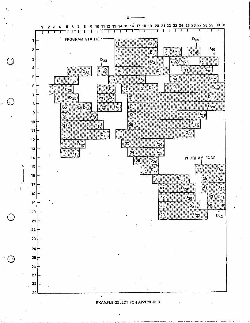
0 .. ' ..

o

0'"" , "

11-

2r-.

x ,.

1 2 3 4 5 6 7 8 9 10 1112 13 14 15 16 17 18 19 20 21 22 23 24 25 26 27 28 29 30 31 J I I I I I I I I I I I I I I I I I I I I I I I I I I I I I

EXAMPLE OBJECT FOR APPENDIX C

- .. '''"'''''''~----'',.., ·~~·'~"':!"'~''''''r_~''''---.-'''I,.,.-~ .... -..... ..-.-........... , •. J''~.'~_'''''-''-'''''''_'''''''''"7'~ ..... __ .~ .. ~_ ...

....

o

0·/ , '~,-'~

BELLCOMM. INC.

Appendix D

Data Storage Estimates for Method II

An analysis on \<lhich memory data storage requirements are based is given here. The symbols used are ~, the n~er of objacts in a frame; L, the number of lines in a frame; e, the number of elements or points of interest in a frame; LK, the

numbar of lines per object.

The number of storage words required to store a master list of points is equal to the number of points of interest in

i=</> a frame, that is MI = e = L

. i=l (area of object i) •

The list of line segments, prepared from the master list,of points, contains the x and y coordinate of the first point of each line and its total length. Two words per line segment would be sufficient to store the information. Hence, the number' of storage words required 'is equal to twice'the number of lines in a frame,or M2 = 2~.

In the process of defining an object, it is required to keep a list of lines belonging to an object. The data storage is then equal to the number lines ,per object or

K=4> L

K=l

. Also while defining an object, the program stores lines in a secondary list. This is a temporary list and once an object is completely defined, it is no longer required. The amount of storage required vari~~ with the shape of an object but should not take more than half the number of lines in the object with the most lines, or M4 = 0.5 (max. LK). For

simplici ty, ~. t is conservatively assur..ed that this function will take no more than half the number of lines in a frame; M4 = O.SL.

.,

I

Bellcomm, Inc. Appendix D (Contd.) 2 -

~ Once the object is defined the memory would store \;3) about 20 parameters, each occupying one data storage word.

o

0 " , "

o

The total number 'of data words is simply twenty times the number of objects in a frame, or M~ = 20</>.

Hence, the total data storage requirements for a frame is the sum total of all the above numbers:

5 M = [. M. = e + 2L + L + O. 5L + 20· </>

i=l ~

= e + 3.5L +20·</>,

Let AI = area of flares of importance I. If we assume

that flares have square configuration~ then we can approximate the number lines per object, LK, as vAl. If all flares in a , frame have the same importance, then x

But

So

The the

M = e + 3.5</>/AI + 20·</>

e = </>AI

M = </>AI +,3.5</>/AI + 20·</>

= (AI + 3.5 IAI + 20)</>

formula can be adapted for rectangular shape flares by following:

a. For a flare elongated vertically: Let y = px, where p is a positive iiteger. the number of lines per flare is ~ AlP and

Then

M = (AI + 3.5 IAI + 20)'</> + 3.5</> (/p-l) IAI

Y

-. x,

y

.. .

. .

o

0, , ,

o

Belh::omm, Inc . Appendix D (Contd.) - 3 -

or

b.

or

For Let the

a flare elongated horizontally: x = qy where q is a positive int~er. Then . x number of lines per flare is '" (gr and T"'"[-------""'1]y

M = (Ar + 3.5 /Ar + 20)~ - 3.5~ (1 - ~) /Ar

Ici

M = (Ar + 3.5 /Ar + 20)~ ;q

Table 4 contains some of the computation based on the above fo~mulation as to how the memory requirements change with the change in the flare's shape. This change is computed for a single flare but can be adapted to any number of flares by simply multiplying the correction factor by the total number of flares in a frame.

, >, , (', ' , . ,I .,. \ ~,

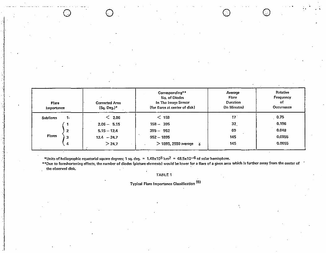
1

J ;,1

·C\ V o

Flare Corrected Area Importance (Sq. Deg.)·

Subflares 1- < 2.06

g 2.06 - 5.15

5.15-12.4 Flares 12.4 - 24.7

>24.7 , -- -----

Corresponding·· No. of Diodes

In The Image Sensor (for flares at center of disk)

<158

158 - 395

395 - 952

952 -1895

> 1895, 2550 average ~

0. V

Average Flare

Duration (In Minutes)

17

32

69

145

145

*Units of heliographic equatorial square degrees; 1 sq. deg. = 1.48x108 km2 = 48.5x10-6 of solar hemisphere.

o v

Relative Frequency

of Occurrence

0.75

0.196

0.048

0.0055

0.0055

**Due to foreshortening effects, the number of diodes (picture elements) would be lower for a flare of a given area which is further away from the center of the observed disk.

TABLE 1

Typical Flare Importance Classification (6)

, . . \

/ !

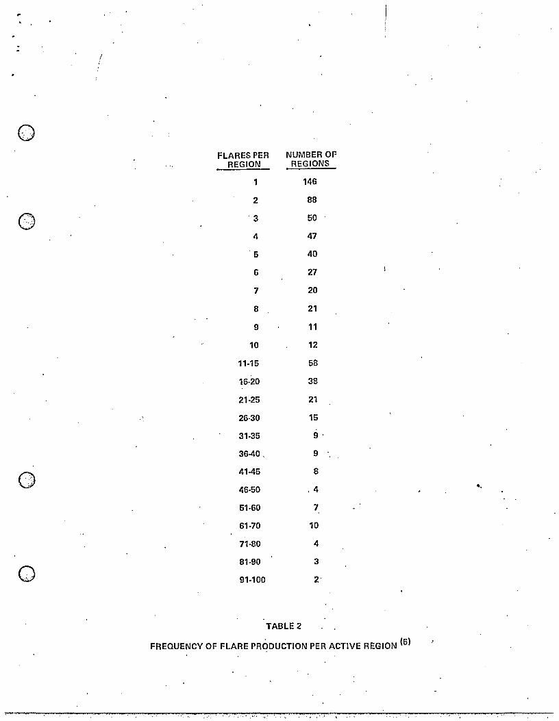
0 ' ..

FLARES PER NUMBER OF REGION REGIONS

1 146

2 88

0 '3 50

4 47

5 40

6 27

7 20

8 21

9 11

10 12

11·15 58

16·20 38

21·25 21

26·30 15

31·35 9'

36·40, 9

0 41·45 8

'" ". 46·50 ,4 ".

51·60 7

61·70 10

71·80 4

81·90 3

0 91·100 2'

TABLE 2

FREQUENCY OF flARE PRODUCTION PER ACTIVE REGION (6)

,@," t ., 'J

"

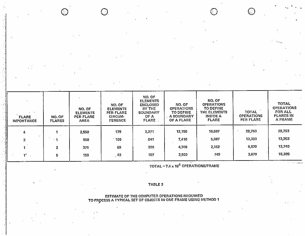
FLARE IMPORTANCE

",

.' 4

2

1 ,

1-

~

I

.

A V

NO. OF FLARES

1

. 1

2

5

.

NO. OF ELEMENTS

PER FLARE AREA

2,550

950

375

150

' " o

NO. OF ELEMENTS PER FLARE

CIRCUM-FERENCE

179

. 109

69

43

NO.OF ELEMENTS ENCLOSED

BYTHE BOUNDARY

OFA FLARE.

2,371

841

306

107

NO.OF OPERATIONS TO DEFINE

. ABOUNDARY OF A FLARE

12,156

7,416

4,708

2,930

tf'\ V

NO. OF OPERATIONS TO DEFINE

THE ELEMENTS INSIDE A FLARE

16,597

5,887

2,162

749

TOTAL = 7 ~4 x 104 OPERATIONS/FRAME

TABLE 3

ESTIMATE OF THE COMPUTER OPERATIONS REQUIRED TO PR9CESS A TYPICAL SET OF OBJECTS IN ONE FRAME USING METHOD 1 . .

~ V

TOTAL OPERATIONS PER FLARE

28,763,

13,303

6,870

3,679

..

TOTAL OPERATIONS

FOR ALL FLARES IN A FRAME

28,753

13,303

13,740

18,395

"'-

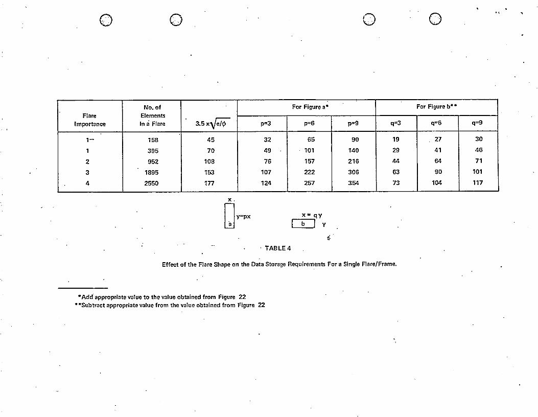
o o o

No. of For Figure a* Flare Elements

Importance In a Flare 3.5 x.y;ii" p=3 p=6 p=9 q=3

1- 158 45 32 65 90 19

1 395 70 49 101 140 29

2 952 108 76 157 216 44

3 1895 153 107 222 306 63

4 2550 177 124 257 354 73 -

x.

Dv-ox x= qy

b ] Y

({,

. tABLE 4

Effect of the Flare Shape on the Data Storage Requirements For a Single Flare/Frame.

"Add- appropriate value to the value obtained from Figure 22 **Subtract appropriate value from the value obtained from Figure 22

0,----'-

., "

For Figure b**

q=6 q=9

27 30

41 46 I I

64 71 I

90 101

104 117

C\ V o

FOR ACTIVE PERIOD (1957)

NO.OF NO.OF NO.OF FLARE FLARES FLARES FLARES

IMPORTANCE PER YEAR PER MONTH PER DAY

4 13 2 1

3 84 17 1

2+ 26 5 1

2 445 118 22

1 4,007 1,067 200

1- 13,725 3,627 675 -

TOTAL 18,300 4,826 900

----- --- --- -- ---

TABLE 5

Ft:ARE STATISTICAL DATA OF THE SOLAR CYCLE NO. 19

0,·-- o ..

---

- FOR PASSIVE I PERIOD ,

(OCT. 1954 ' THROUGH

SEPT. 1955)

NO.OF FLARES

PER YEAR

4

38

126

168

-- --

'.

1 'J 1

o 0,

\ ~ ; ...

YEAR F\ N NR

1954 4.4 16 42

1955 J38.0 294 ' 544

1956 141.7 2,020 3,003

1957 190.2 3,436 14,226 1 1958 184.8 ,3,361 3,536

1959 159.0 3,704 3,924

1960 112.3 2,207 2,386 ..

R '= SUNSPOT NUMBER

N = OBSERVED NUMBER OF FLARES

NR = REDUCED NUMBER OF FLARES

I = AVERAGE OBSERVED FLARE INCIDENCE PER HOUR

1* = CORRECTED FLARE INCIDENCE PER HOUR

TABLE 6

FLARE INCIDENCE (6)

o 0',' ,~-..

'.

I 1*

.017 .005

.062 .047

.343 .294

.481 .440

.403 .391

.447 .433 -

I .272 .263

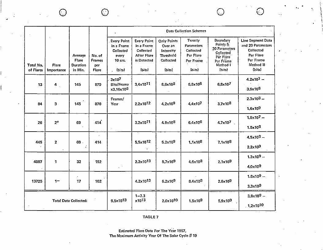
o ~l

-

Averasg Flare

Total.No. Flare Duration of Flares Importance in Min.

13 4 145

84 3 145

26 2+ 69

445 2 69·

4007 1 32

13725 1- 17

Total Data Collected:

0\ V

No. of Frames

per Flare

. Every Point in a Frame Collected

every 10 sec.

(bits)

Every Point in a Frame Collected

After Flare is Detected

(bits)

Data Collection Schemes

Only Points Twenty

Over an Parameters Intensity Collected

Threshold Per Flare Collected Per Frame .

-

(bits) (bits)

_ 3x107

870 Bits/Frame 3.4x1011 8.6x103 6.8x106

x3.16x106

Frames/ 870 Year 2.2x1012 4.2x109 4.4x107

414 3.2x1011 4.8x108 6.4x106

414 5.5x1012 5.2."(109 1.1xloS

192 2.3x1013 8.7x109 4.6x108

102 4.2x1013 6.2x109 8.4x103

1-7.3 9.5x1013 x1013 2.6x101O 1.5x109

TABLE 7

Estil1'.ated Flare Data For The Year 1957, The MJximum Activit'! Year Of The Solar Cycle # 19

o

Boundary Points &

20 Parameters - Collected

Per 'F/are-Per Fr"1ime Method I

(bits)

6.8x107

3.7x108

4.7x107 .

7.1x108

2.1x109

2.6x109

5.9x109

o v

Line Segment D<lta and 20 ParOl meters

Collected Per Flare Per Frame iVtllthod II

(bits)·

4.2x101-

3.6x108

2.3x108 -

1.6x109

1.8x107 -

1.Sx10S

4.5x108 -

2.2x109

1.3x109 -

4.0x109

1.8x109 -

3.3x109

3.8)(109 -

. 1.2x101O .-

"

I I

r ~ ~

~ t \

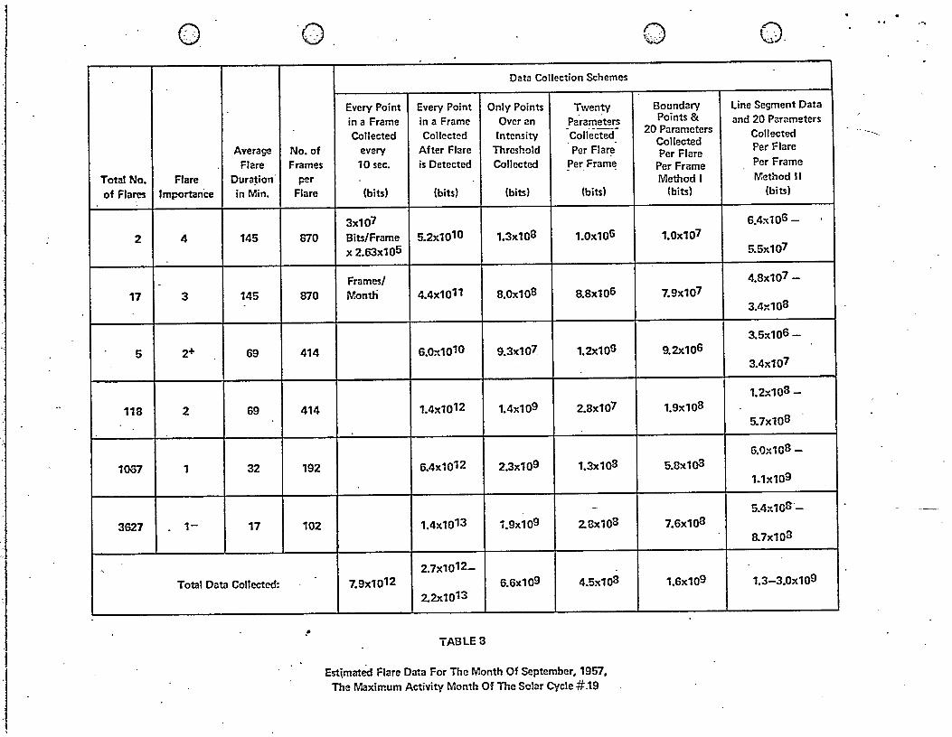
o.

Average Flare

Total No. Flare Duration of Flares Importance in Min.

2 4 145

17 3 145

5 2+ 69

118 2 - 69

1057 1 32

3627 . 1- 17

~

Total Data Collected:

o. Data Collection Schemes

Every Point Every Point Only Points Twenty in a Frame in a Frame Over an Parameters

- 0 __ -

Collected Collected Intensity Collected No. of every After Flare Threshold Per Flare Frames 10 sec. is Detected Collected Per Frame

per Flare (bits) (bits) (bits) (bits)

3x107

870 Bits/Frame 5.2x101O 1.3x108 1.0x106

x 2.63x105

Frames/ 870 lV.ontfl 4.4x1011 8.0x108 8.8x106

414 6.0x101O 9.3x107. 1.2x106

414 1.4x1012 1.4x109 2.8x107

192 6.4x1012 2.3x109 1.3x1oS

-102 1.4x1013 1.9x109 2.8x108

2.7x1012-7.9x1012 6.6x109 4.5x108

2.2x1013

,. TABLES

Esttmated Flare Data For The Month Of September, 1957, The Maximum Activity Month Of The Solar Cycle # .19

Q o. .-.

Boundary Line Segment Data Points & and 20 Par<lmetcrs

20 Parameters Collected

Collected

Per Flare Per Flare ........

Per Frame Per Frame

Method I lV'.cthod II (bits) (bits)

6.4x106 -!

1.0x107

5.5x107

4.8x107 -7.9x107

3.4x108

3.5:<106 -9.2x106

3.4x107

1.2x108 -1.9)(108

5.7x108

6.0x108 -5.8x103

1.1x109

5.4::108 .-7.6x108

8.7x108

1.6x109 1.3-3.0:<109

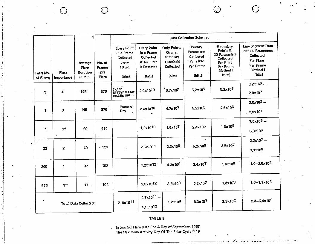
o 0', , ,

Avera£9 No. of Flare Frames

Tot::J I\~. Flare Durlrtion per of F1aro, I mport.."'nCe in Min. _ Flare

1 4 145 870

1 3 145 870

1 z+ 69 414

22 2 69 ·414

200 1 32 192

675 1- 17 102

. Total Data Collected:


Every Point Every Point Only Points Twenty in a Frame in a Frame Over an Parameters Collected Collected Intensity Collected

every After FI<lre Threshold . Per Flare

10!:ec. is Detected Collected Per Frame

(bits) (bits) (bits) (bits)

3x107

BITS/FRAME 2.Gx101O 6.7x107 5.2x105 x8.65x103

Frames! :Day 2.6x101O 4.7x107 5.2x105 . -

-1.2x1010 1.9xl07 2.4x105

2.6,,1011 2.6x108 5.2x1 OS

1.2x1012 4.3;(108 2.4x107

2.6x1012 3.5x108 5.2x107

4.7x1011 -2.6x1011 1.2x109 8.3x107

4.1x1012

TABLE 9

Estimated Flare Data For A Day of ~p~mber. 1957 The Maximum Activity Day Of The Solar Cycle # 19

r:\ V

Boundary Points &

20 Parameters Collected Per Flare Per Frame Mathod I

(bits)

5.2x1 oS

4.6x105

1.9x10-5

3.5x107

1.4x103

1.4x108

2.9x103

--------

A V

line Segment Data and 20 Pllrametcrs

. Collected

Per Flare -----Per Frame Method II

'bits}

3.2x10G -

2.8x107

2.Bx10S -

. 2.O:t107

7.0x105 -

6.8x106

2.2x107 -

1.1x103

1.0-2.0x108

1.0-1.7x103

2.4-5.4x103

I

-.- ----- -------

. . -, -"'- ~ .... ", •• -- --~ ~-.""", , """,,,."~' ".- ,"," ......... -"';:-~~-?- '~"""'''''''':''''--;-:'''> ~"" -: .......

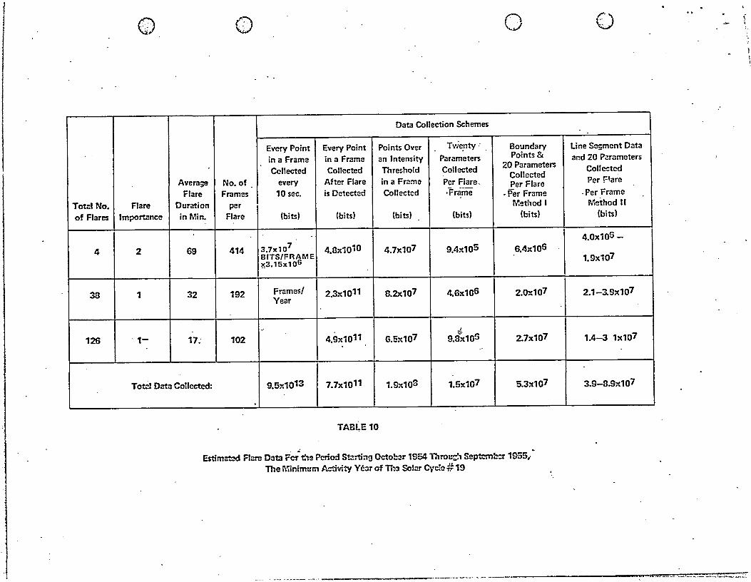
I Q>. ,'"" -" o o o


Every Point Every Point Points Over Twe.nty· , Boundary line Segment Data in a Frame in a Frame an Intensity Parameters Points & and 20 Pzrameters ecllected Collected rnreshold Collected 20 Parameters Collected

Average No. of After Flare in a Frame Collected

Per f-lare every Per Flare. Per Flare Flare Frames 10 sec. is Detected Collected .Frame • Per Frame .Per Frame

Total No. Flare Duration per Method I lV'oethod II of Flares Importance in Min. Flare (bits) (bits) (bits) (bits) (bits) (bits)

4.0xl0S - I 4 2 69 414 3.7x107

4.l3x101O . 4.7x107 9.4x105 6.4x106 I

BITS/FRAME 1.9x107 x.3.15x106 i

38 1 32 192 Frames! Year

2.3x1011 8.2x1 07 4.6x1n5 2.Ox107 2.1-3.9x107

J t{

126 ' 1- 17: 102 4.9xl011 6.5x107 9.8x105 2.7x107 1.4-3 1x107 -

Totcl Data Co-Ucctcd: 9.5x1013 7.7x1011 1.Sx103 1.5x107 5.3x107 3.9-3.9x107

-- - .~- ~

TAB~E10

Estima1ed flare Dati Fc-i t!1e Period St:!rting October 1954 Throu~ ~pt::mb 1955,: The Minimum A...'"tivity Year of Ti~ Sclnf Cycle # 19

'j • ______________ . ________ .• _- u = .. , _ .... _ ..... 5. _

I

O· .. ' ~.

o

(FILAfV1ENT)

0,,>·· "

N

REGION OF NUCLEAR ENERGY REACTION:·

H~He

CONVECTION LAYER

". FIGURE 1 • THE SUN AND ITS MAIN FEATURES

(TAKEN FROM THE "HANDBOOK OF GEOPHYSICS AND SPACE ENVIRONMENTS" AIR FORCE CAMBRIDGE RESEARCH LABORATORIES)

.. !,

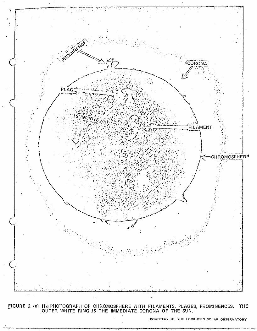
C" "

c'

;'J

fiGURE 2 (a)

~ . "," . \ , .',

'.'

,,<' I

'. r, ,. " Jf

, J, ~ .. '. 'r

" .

.',..,

: ~.,','..,~.<.),;(:~.<~/ '.;' II ,

'"

'" "' .... , , ~'

, -t,

'.) .J "'-

,., . ,

~'c;:!l CH ~9~9.~lE R E

','

, , , ,

( :

H CI. PHOTOGRAPH OF CHROMOSPHERE WITH FILAMENTS, PLAGES, PROMINENCES. ,OUTER WHITE RING IS THE IMMEDIATE CORONA OF THE SUN.

THE , '

COURTESY OF THE LOCKHEED SOLAR OBSERVATORY

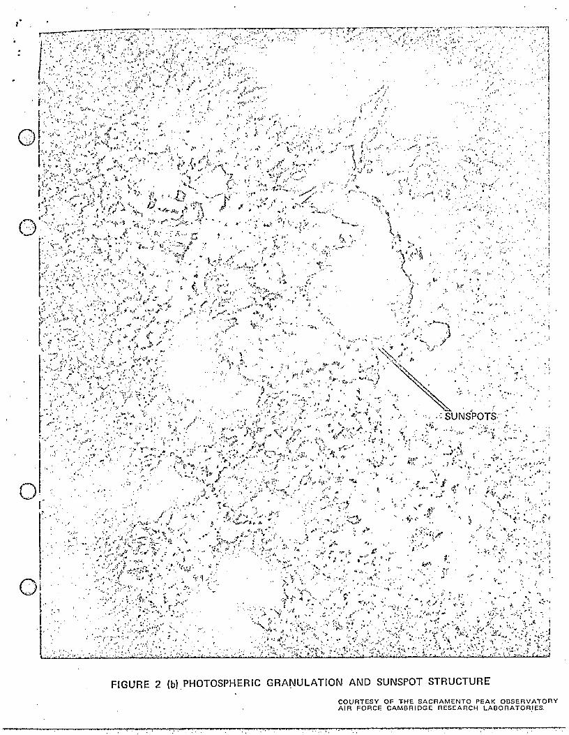
r or L

':~" • r - '.

'. -. " ,,':': ..-.~.' ":": .:.';".,.;l",. ",' ,;'-' ..... ,~, ... ' .:~~ • .:.,' ,-' .;.i<.l":""""

.~ . .,: r" ;: .. ' .... ~ 'f ,:' -'"

, i \ , .

.'" j .. ( . /

" " .' , ');'

.' , ,';

.. j' ..... ,"

" '1

" ,.,,'>

"

i

'. " ."

, "

"

FIGURE 2 (b) PHOTOSPHERIC GRANULATION AND SUNSPOT STRUCTURE , '

~, e ,_ I, , ," ~ I

COURTESY OF ,HE SACRAMENTO PEAK OElSERVATORY AIR FORCE CAMBRIDGE RESEARCH LABORATOR,IES,

,I,¢ ." ,k

o

o

o

" '

".

FIGURE 3 (a) Ha PHOTOGRAPH 'OF THE SOLAR FLARE, PLAGES, AND FILAMENTS

COURTESY OF ThE SAChAMENTO PEAK OBSERVATORY AIR FORCE CAMBRIDGE RESEARCH LABORATORIES

.. , ,

0',' " '

o

o

.,,' , ",,'/

,r ;(A"~::~f': ,;

I,ft' ,

..:.' . :

'" ',.-

" r',':- ~ ":.,:

~ ~ . \ . ',::; "'~. ,':',':-;' ,:.,:-,/ ... ,

( '# ,.-t·'

FIGURE 3 (b) H (J. PHOTOGRAPH OF A LARGE FLARE

COCJRTESY OF THE SACRAMENTO PEAK vBSERVATORY AIR FORCE CAMBRIDGE RESEARCH LABORATORIES

, I, \. ,p

I I

1

r '·1

.1

1 I

0. -",:

EARTH'S MAGNETIC

FIELD

GALACTIC COSMIC RADIO' NOISE SIGNAL'

STRENGTH

GALACTIC COSMIC RAY

INTENSITY

SOLAR PROTON.

INTENSITY:

LOW-FREQ. SOLAR RADIO

EMISSION'

HIGH-FREQ. SOLAR RADIO

EMISSION .

. FLARE LIGHT, . ULTRA-VIOLET

AND X-RAY

Q :;:'

SUDDEN. COMMENCEMENT

0 , - 0 - ,

AURORAE ~ .,.

r---------~----------------------------------C --------------~ . POLAR CAP AURORAL RADIO BLACKOUT' ABSORBTION ;,--' __ ------,

~ ~~r -

--------- C

10-30% . 1 .DECRE~~E~

FLUX OVER POLAR CAPS. ---- FLUX AT FORBIDDEN LATITUDES

MAY BE 1000- TIMES', .,

., G.C.R. FLUX ",

'.

2 4 6 8 10 12 14 16 18 20 22 24 26 28 30 32 34 36 38 40

TIME (HOURS)

FIGURE 4 (a) - TIME SEQUENCE OF MOST OF THE IMPORTANT CHROMOSPHERIC FLARE EFFECTS OBSERVABLE AT THE EARTH

(TAl<EN FROM NASA TN -700)

. -.

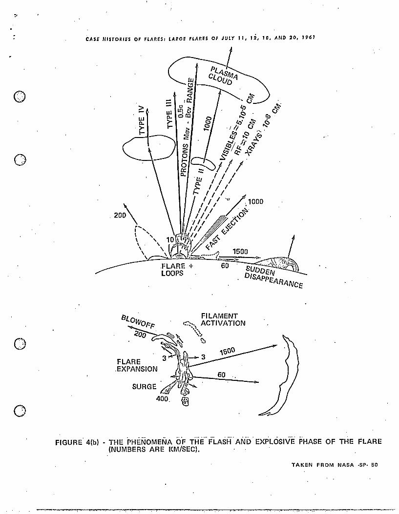
0> "

0,' <,

O~ J,'

CASE HISTORIES OF flARES: LARGE FLAr.ES OF JULY Jr, 12, HI, MID 20, '96'

20~

::: w 0.

,. ... I ,

\ " \ , \. ,

--

\ \ \ \

\

.FLARE + LOOPS

8L . FILAMENT

~OWOf:f: ' c~:. ACTIVATION

.\ . <00 ' ~~ \~,

60 "

FIGURE' 4(b) • THE PHENOMENA OF THE'- FLASH-' AI\fD' EXPLOSIVE PHASE OF n-iE FLARE (NUMBERS ARE J<M/SEC). .

TAKEN FROM NASA ~p. 50

0,',) , '

()

_-'-"""~~:-:"!C-7"'7"-:--:''''::' 'c' ""''T''''~' op-:;r--:'.-~; ~'''''''',i:':-r>"",,; ... ,,-, -'''''''~'~'' ,c:":., , ~,~,!~~~~;,r~>:,,~""'~. , ,,', , "

..... ,

FIGURE 5 (a)

. ~ ': ."'~ I .... ,"" .. ,,~ •

-'

O'H., .. • • • _

"

~ , \,A' '{

'A'f iii 0/./' ! I ,.""",Jl::.,,

H ct PHOTOGRAPH OF THE CHROMOSPHERE SHOWS PLAGES AND BLACK FILAMENTS. ' , " , ..

COURTESY OF THE SACRAMENTO PEAK 'oBSERVATORY AIR FORCE CAMElRIDGE RESEARCH LABORATORIES

. . '

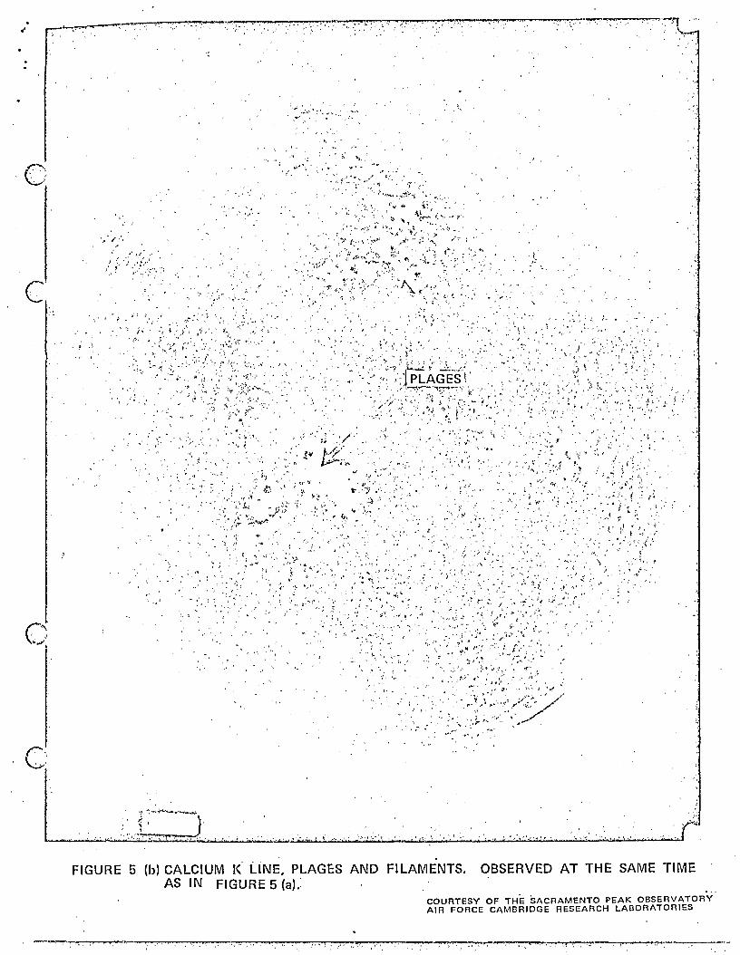
C"· , " ~1

c

r·\ \..:..v,

" ,

, ,J

,. . " "1 ;.:

, t:.,

, '\'

- '~~> ~ ... "t _:: ;"',

.,:. '

"J ":-~-r-................. .....i

.... ~ ..... _ ............ ~~."' .. :;.;,.:.:.: ... ~:.., ~ .. 'W::.·" ) .. ,.

'.'-'

, ~l • : __

. /,' , .'

;",

, ,,'

" ,~ :.. '\'1.

~.,~ ".., , \ I

',' ,

,1('

\ t~ ~ :, "' . '). . ;

-. ~. ":1"': ~I. ~ 'I'"

". ', .. ~ .:

" ,

.. '

.' J.'

;', .~

. ~ ,

. ,..' ..

" ,'.: '.'

. i ~. I' "

, "

.;

"

FIGURE 5 (b) CALCIUM I< LiNE, PLAG£:S AND FILAMENTS. OBSERVED AT THE SAME TIME AS IN FIGURE 5 (a).:

COURTESY OF THE SACRAMENTO PEAK OBSERVATORY AIR FORCE CAMBRIDGE RESEARCH LABORATORIES

\ <~

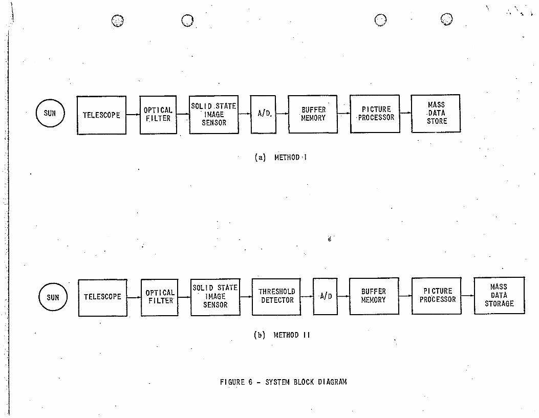
8

8

q ~@

TELESCOPE

TELESCOPE

OPTICAL I--

~~LTER

OPTICAL I-- FI LTER·

o

SOLI D . ST ATE A/D. BUFFER f- . IMAGE I-- f-- I-:-

SENSOR MEMORY

(a) METHOD, I

@,

SOLI D STATE THRESHOLD ·A/D . IMAGE .- f-I-- f- -DETECTOR

SENSOR

(b) METHOD"

FIGURE 6 - SYSTEM BLOCK DIAGRAM

o

P.ICTURE I"-. PROCESSOR

BUFFER f-.

MEMORY

n ~,J

MASS ·DATA STORE

PICTURE PRO"cESSOR

\ \ • \ "'.10.

I

NASS I-- DATA

STORAGE

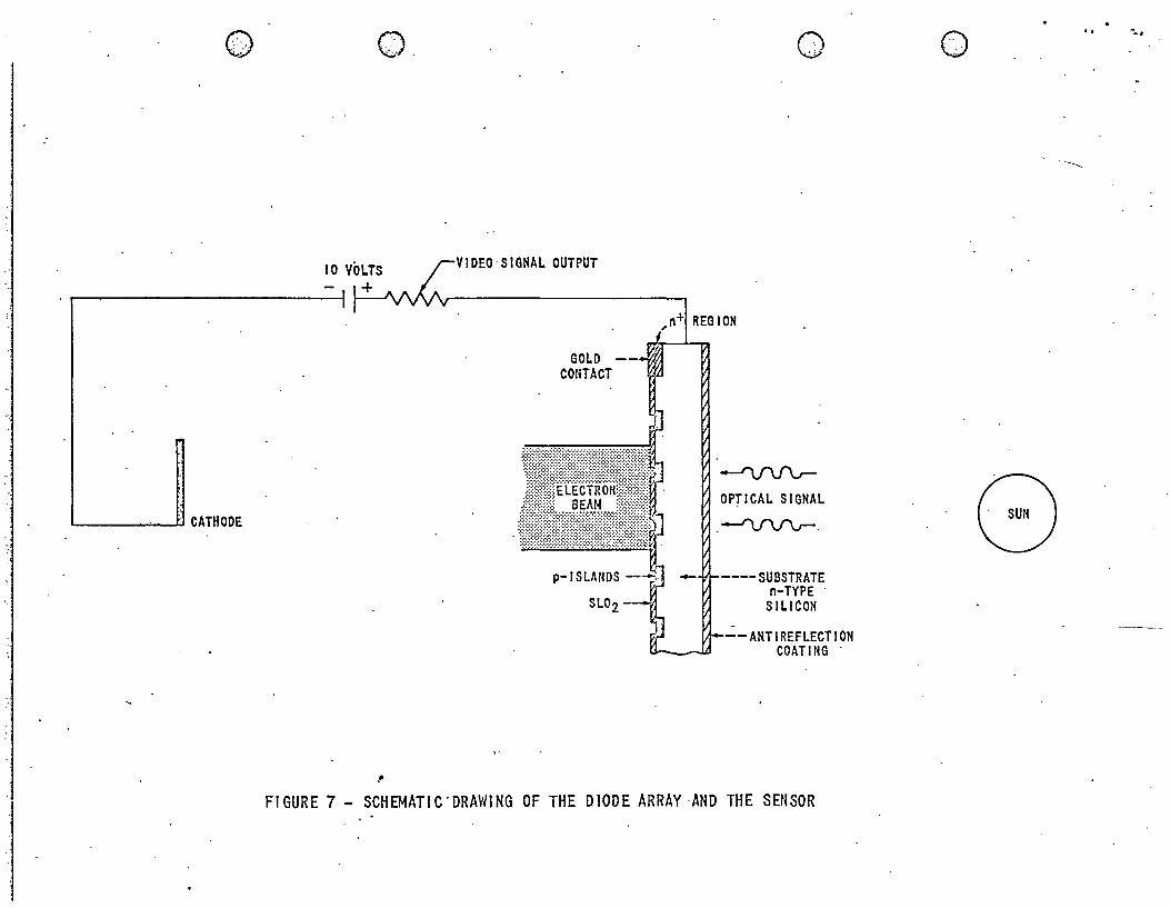
(0 v...y

L..-_____ .i.J'I CATHODE

(7\ \6,) .

..

IDEO'SIGNAL OUTPUT

GOLD COnTACT

o

REGION

-'VV\.rOPTICAL SIGNAL

--rvv\r--

_-wl----- SUBSTRATE n-TYPE .

SILICON --- ANTI REFLECTION

COATING .

FIGURE 7 - SCHEMATIC·DRAWING OF THE DIODE ARRAY ·AND THE SENSOR

o II

-~

0)

~.

~. ~

.::t 2

> !:: > t-en 2 w en

1.0

.0.8 0.6

0.4

0.2

0.1

0.08 0.06

0.04

0.02

o v o

UNITY COLLECTION EFFICIENCY

SILICON TUBE LOW "S" SURFACE

VIDICON 8134

---- EYE RESPONSE ----

o 0'·' -~ :,

-,

0.01 " 0.4' 0.5 0.6 0.7: 0.8 0.9

WAVELENGTH,.A., IN MICRONS

HCJ1 = 0.6563 CA II. I< =' 0.3934 (13)

FIGURE 8 - COMPARISON OF 1 MIL SILICON TARGET WITH ANTIMONY TRISULFIDE TARGET'

...

1.0

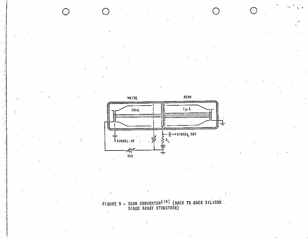
o o

-l-

o

WRiTE READ

." IOnA I IJ..L A" ~rr"WK,r1i1;;WMti0~.L. ~4--. I

TS,GNAL.,N . ..It Pf-'SIGHA" OUT

-------~~.t' 1-2kV -i

FIGURE 9 - SCAN CONVERTER(16) (BACK TO-BACK SI~ICO~ , DIODE ARRAY STRUCTURE)

0""" ",'

.. "-

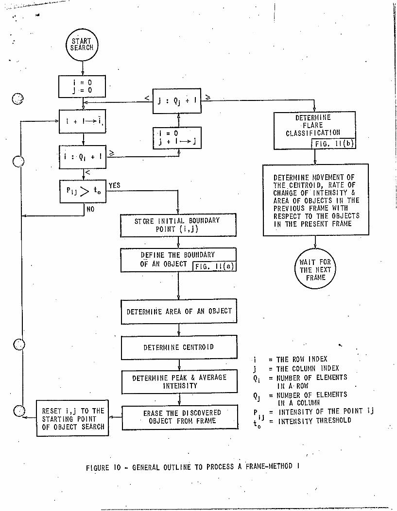
START SEARCH

i = 0 j .= 0 n v t<------<-t j : QJ + I J-;i:::.~-":""---------...., t

I ~

i + I~i ,

J (. i : . Qi + I ~

!< PiJ> to

YES

I NO

~ RESET i ,j TO THE ~ STARTING POINT iq.

OF OBJECT SEARCH

STORE INITIAL BOUNDARY POINT (i,j)

DEFINE THE BOUNDARY OF AN OBJECT I FIG. II (a)

DETERI,1I t~ E AREA OF AN OBJ ECT

DETERMINE CENTROID

DETERM I tI E PEAK & AVERAG E INTEUSITY

ERASE THE DISCOVERED OBJECT FROM FRAME

DETERMINE . FLARE

CLASSIFICATION IFIG.II(b)

DETERMINE MOVEMENT OF THE.CEtlTROID, RATE OF CHANGE OF' INTENSITY & AREA OF OBJECTS IN THE PREVIOUS FRAME WITH RESPECT TO THE OBJECTS IN THE PRESENT FRAME

..l

(~'/AIT FOR THE NEXT

FRA~1E

. j = THE ROW INDEX

to •

j = THE COLUMN 1UDEX Qi = NUMBER OF ELEMENTS

IN A·RO\'! QJ = HUMBER OF ELEMENTS

IN A COLm~H P

iJ = INTENSITY OF THE POINT ij

to = I KTEHS ITY THRESHOLD

FIGURE 10 - GENERAL OUTLIN~ TO PROCESS A ~RAME-METHOD

------------------------------------~-----.~ .. ~~.

~. j

.' .

'\

)

~)

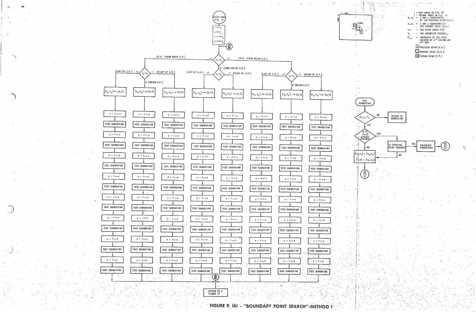
\ J

._-/

~~

(LEFT OF C.P.)

(X" Y,)':" (X, y)

(P.P. ISROW ABOVE C.P.)

(R I uHT OF C. P. ) (LEFT OF C.P.)

(x"Y,) _ (X,y) (x"y,) _ (X,y)

"

''''. ~ i :~~ .. " ! ~{,

y.r~X~---== ______________ ~

j-X , I-I-Y ,

-I (P.P. IS ROW BELOW C.P.)

-I (RIGHT OF C.P.) (LEFTOrc.p.) .1 i

..,:'

.t

-I (RIGHT or c.p.). i

(x,'Y') _ (X,y)

-! ~

FIGURE 11 (A) IIBOUNDARY' POINT SEARCH".:;METHOD 1 '.' 'r-_'

.~. X,1 •

I

~I i j 1

I , 1

i

I I

! I, I

- _ ,r i r I

¥: I,

t'. I . : .'

i . !

>1 f.

t 1 .. c_; ,

"

I t >

" ~ i

1 I

·1 , ! I

~!.. ~ - -?

...::.. ~

-~- ,

'." --~:-

Xp .Yp

Xc I Yc

x,l

to P '.1

: ROW INDEX IN FIG. Ie : COLUMN I NDEX IN FI G. ;0

x AND y COOROINATES OF THE PREVIOUS PGIHT'??,.;

x AND y COORDINATE C, THE CURRENT POIH (C.P.; THE POINT UN"ER TESI

THE INTENSITY THl,"SH~_j

INTENSITY OF THE POI~T LOCATED AT x" CO:'~'llI ..... ; ,'

0 ROW

9PREVIOUS POINT(P.P.)

OCURRENT POINT (C.P.)

mn FUTURE POINT (F.P.)

,.

1,

'- ,t

i '. I f f i I

<w

:

0 ,;:.,

\ /'-....., «, )

"-t)'

0 ' .. "

0 . "

I

YES

ENTER

( FROM I

FI G. 10

< i = 0

i + I __ i

IS THE ,AREA OF THE OBJECT i ~ AREA OF ,A FLARE OF IMPORTANCE 2

NO <,

I S THE AREA OF THE OBJECT' i ~ AREA OF A' SUB-FLARE OF IMPORTANCE 1-

NO

I S THERE ANY CLUSTER FORMATION OF FLARES OF IMPORTANCE I

NO

IS THERE ANY OBJECT LEFT

YES

YES

YES' 'FLARE ALERT' TURNS ON

NO I \

~/GURE //(b) - TO DETERMINE FLARE CLASSIFICATioN-METHOD ,I ','

-RETURN )

TO FIG. 10

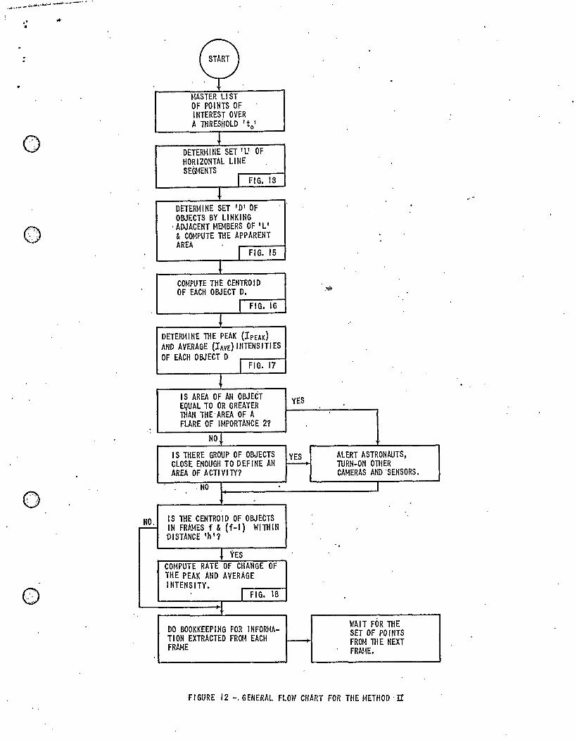
.t ,.,

«

e . MASTER LIST OF POINTS OF INTEREST OVER A TIlRESi-JOLD 'to'

o ~ DETERM !tIE SET 'L' OF HOR I ZONTAL LI HE SE~ENTS

I FIG. 13

J DETERM!tlE SET '0' OF . OBJECTS BY LINKING

, ADJACENT MEMBERS OF 'L' & COMPUTE TIlE APPAREHT AREA I FIG. 15

~ COMPUTE THE CENTROID OF EACH OBJECT D. :~

I FIG. 16

~ DETERMltiE lllE PEAK (IPEAd AND AVERAGE (rAVE) ItlTENS JTI ES OF EACH OBJECT 0 I FIG. 17

J I S AREA OF AN OBJECT YES EQUAL TO OR GREATER THAN THE' AREA OF A FLARE OF IMPORTANCE 2?

Not

IS lllERE GROUP OF OBJECTS ~

ALERT ASTRONAUTS, CLOSE ENOUGH TO DEFINE AN TURN-ON OTHER AREA OF ACTIVITY? CAMERAS AND 'SENSORS.

110 I t ,

~ IS TIlE CENTROID OF OBJECTS IN FRAMES f & (f-I) WlllllN I

"DISTMICE 'h'?

. ~ YES COMPUTE RATE OF CHANGE OF THE PEAK MID AVERAGE I NTEIISITY.

I FIG. 18

t

DO BOOKKEEPING FOR IHFORHA- WAIT FOR THE SET OF POlrlTS TION EXTRACTED FROM EACH r---- FROM THE HEXT FRAME FRAHE.

FIGURE 12 -. GENERAL FLOW CHART FOR THE METHOD,'II

,. ,.,

EtHER MASTER LI ST

OF POINTS

N = TOTAL NO. OF POINTS IN THE MASTER LIST

i,j,k =·ltlDEX·ES

'Lk = j.th ELEMENT OF kth LItlE J ! SEGMENT

£ L , I = Y CO 0 R D I tI AT E,

€J j '= I

.eL 2 = x COORD I NATE AND

tL 3 = IrHENSI TY OF Lt

o

O· . " j .-.

k = I

j = I

Sj'= jth ENTRY IN THE MASTER LIST

5 I ,I;15' j ,2 = Y·AND ;t.COORDINATE OF Sj

J '= DENOTE THE TOTAL NUMBER OF . k ELEMENTS IN THE kth LINE SEGMENT

___ N __ ~j_:_O~~<~----~ ___ j-+ __ J_K_'~~ !~

. t ~ , 1 : s 1 , I I-::I=.L.-.. ________ ~

j--.J K k + I~k

Ak II. s =I=-L J ,2+' 1,2 't-=------otJot

I FIGURE 13, - TO DEFINE LINE SEGMENTS - METHOD IT

"

,..

-......" ~

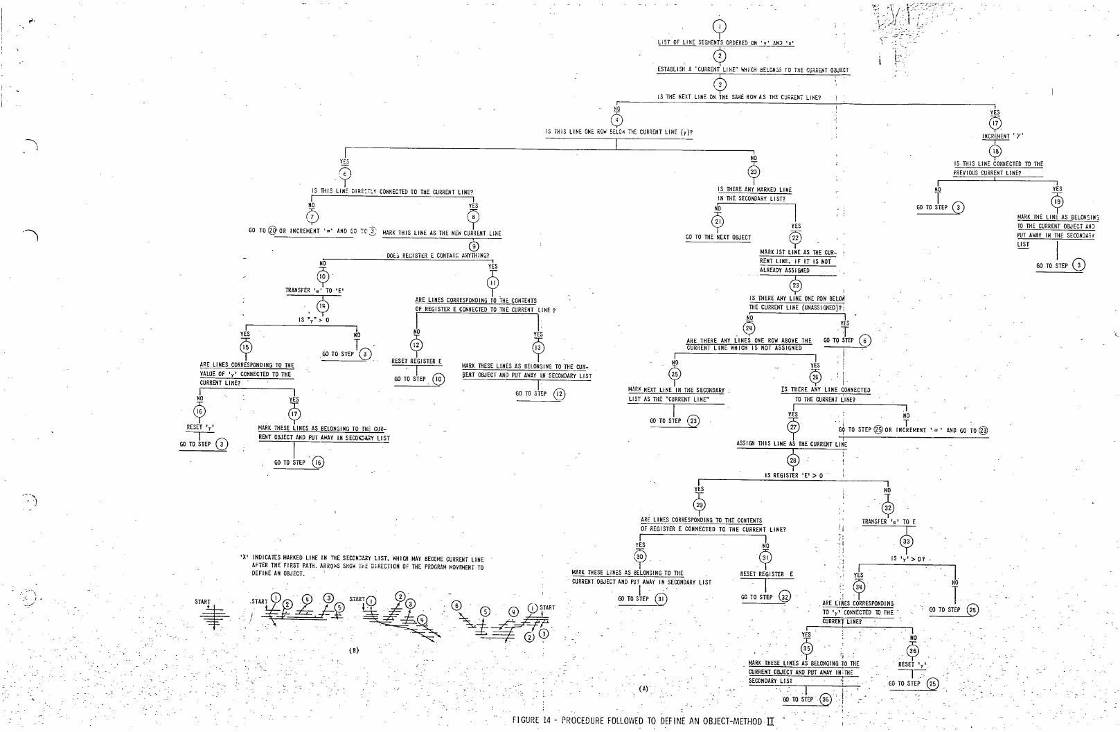
'1

~-", . )

_ i ", , I --~~

Q II ST OF II NE SEGI~E($ORDERED ON 'y' AN) 'x'

ESTABLISH A "CURRENT LINE" ~1iICH BELCN~S TO THE CUilRENT OBJECT

4) IS THE NEXT LINE ON THE SAME ROW AS THE CUi\RENT LINE?

~; '\";' i/-;'C"'-'-'" '\;);·~'.(::-:~r·'= - . .;-'

t - .' t::~_~- -l~r_

r I 1

0' 0 IS THIS LINE ONE ROW 5ELO~ THE CURRENT LINE (y)? INCREJ.1ENT 'Y'

------ ---- -I T , ~

@ ~ IS THIS LINE COh."lECTED TO THE

, '~ IS THERE ANY MARKED LINE

PREY I OUS CURRENT II NE? T

I'

T ~ IS THIS LINE DIRE:TcY CONNECTED TO THE CURRENT LINE? IN THE SECONDARY LIST? I I r'-------------, o _ ~ ~ YES

GO TO STEP CD Y MARK THE LINE AS BELONSIHS

TO THE CURRENT OBJECT AN)

GO TO @ OR INCREMENT 'a' AND GO TC' ~ MARK THIS LINE AS THE NEW CU~RENT LINE GO TO THE NEXT OBJECT Cif5 o MARK 1ST II NE AS THE CUR-

DOE:'; REGIST~R E CONTAI:: A:~YTHING? '-"

,~, ~ TRANSFER 'a' TO 'E' y,

ARE LI HES CORRESPOND I NG TO THE

<$> ARE LINES CORRESPONDING TO THE CONTENTS III OF REGISTER E CONNECTED TO THE CURRENT LINE?

IS"y">O I 1: yJs Jo ~NO ~YE5 ~ T· 12 13 Y ,Go TO STEP 0)

, , RESET REG I STER E MARK THESE LINES AS BELONGI NG TO THE CUR-

'I r.;:;'\ ~ENT OBJECT AND PUT AWAY IN SECONDARY LI ST GO TO STEP, ~ , '

GO TO STEP ® VAWE OF 'y' CONNECTED TO THE

CURRENT LI NE? ' I - I

KcNI LINt. IF IT IS NOT

ALREADY ASSI GHED

~ 1

I S THERE ANY LINE ONE ROW BELOIf

THE CURRENT LINE (UNASSI GNED)?;

N'O I ~ YES

,~ 'r ARE THERE ANY LI NES ONE ROW ABOVE THE GO TO STEP 0 CURRENT LINE WHICH IS NOT ASSIGNED

I I

~ ® I MAR~ NEXT LINE IN THE SECONDARY IS THERE ANY LINE CONNECTED

LI ST AS TIlE "CURRENT LI NE" TO THE CURRENT LI NE? r- ,I Y~ , : M ~, ,~

RESET 'y' MARK THESE LI NES AS BELONG I NG TO TIlE CUR-

GO TO STEP @ C? ' ~t TO STEP @ OR INJEMENT 'a' AND GO TO @

~ GO TO STEP 0

".

RENT OBJECT AND PUT AWAY IN SECOIOl.Al' II ST I ' GO TO STEP '@

'X' INDICATES MARKED LINE IH THE SECOH)4l' LIST, WHIC/f MAY BECOME CURRENT LINE AFTER THE FIRST PATH. AR~O""S SHOo Tr.::: DiRECTION OF THE PROGRAM MOVEMENT TO OEF I NE AN OBJ ECl.

I 'G) CD STA?T(j) ,20 , ' ;""lflk.k~ . lCls#~ - CD START @-py~ \..~00

(B)

ASSIClI THIS LINE AS THE CURRENT LINE

$: IS REGISTER 'E' > 0

1 I YES NO

~ ,,~ ARE LINES CORRESPONDING TO THE CONTENTS I TRANSFER 'a' TO E

OF REGISTER E CONNECTED TO THE CURRENT lIHE?: ~ '~

I I;' "y ~,~ ":' IS'y'>O?

yy '.1 I I MARK THESE lIHES AS BELONGING TO THE RESET RE,GISTER E • ~YES. NO CURRENT OBJECT AND PUT AWAY I N SECONDARY II ST

I GO TO STEP ®

(A)'

:, 3q T GO TO STEP GY ' ! ' . -----:--= ,ARE (IUs CORRESPONDING

TO 'yl CONNECTED TO THE'

CURRENT II NE? ' ,n 1

~';. ~' 9,,} -y MARK THESE lIHES AS BELONGING TO THE . RESET 'y',

GO TO STEP

CURRENT OBJECT AND PUT AWAY IN:THE '~ SECONDARY LIST . ,1 ' ,GO TO STEP' @ n

I ., .1,

GO TO STEP@ :..1' ,-,

FIGURE 14 - PROCEDURE FOLLOWED TO DEFINE AN OBJECT-METHOD·II -

@

--'.

PUT AWAY IN THE SECONDARf

LIST

I GO TO STEP CD

'-

, -.!I

-J r

"

.r

YES

-;-)

-~) 1

-I -L '- / \ - / t ;1

I -FIGURE 15 ~~_FLOWCHARTTO DEFINE AN ~'OBJECT"

-- . -- . "-. METHOD n--

,I Ij

ABOVE TO LEtT

'r ,<

- ~ , ,

1 ' I

, -! 1-

, i

,

Q

ll' = Ok r'

"'~ark Lt

,0

nlll , nlO>

N '" ninll)

p

\ ~

,\(~

, !

.- -.-:,..-'

-::/

IVJ=X OF LINE SEGMENTS. LI

.",C:::X OF A~ ASSIGNED LltliE SEGMENT OR CURREN, LINE Of A..' OBJECT Ok

T07AL t-tUM3ER OF LINE SEGMENTS IN A FRAME

··.,JEX OF A REGISTER THAT INCREMENTS WHEN THERE IS:"

lI~E ONE ROW BELOW AND TO THE lEFT OF THE CURRENT LINE

I-\OEX OF A REGISTER THAT INCREMENTS IF T~ERE IS ANY

Ul'oE TO THE RIGHT OF AND WITH THE SAME y INDEX AS THE CURRENT LINE

THE LINE SEGMENT WHICH CORRESPONDS TO THE PR~VIOUS

CURRENT LINE

"' ... fANS Li IS PARr OF Kth OBJECT AND IS PUT AWAY IN THE

SECO~DARY LIST FOR fURTHER PROCESSING.

THE INTEGER FOR INDEXING REGISTERS. e HAS UPPEA

U\fIT aAND b HAS.., AS AN UPPER LIMIT.

THE NUMBER OF POINTS IN THE LINE L' OR D~. THE CURRENT

LINE --

NUM3ER OF POINTS IN AN OBJECT K_

AN I~DEX THAT INCREMENTS EVERY TIME A LINE IS MARKED_

INDEX OF MARKED LINE IN THE SECONDARY LIST AT M.V

PARTICULAR TIME OF THE PROGRAM p CORRESPONDS TO

SOME LIIN THE MASTER lIST_ t

P NUMBER OF OBJECTS IN A FRAME_

,-

!.. :-:.-

, -..... ~ ---' ~'

~;

~

"

~_ l.

I i .

.' ,. .

..

o

0-, "

~ V

EUTER FRO~1

FIG. 15

.I K = I I ~

i = 0 , XK = 0 yK = 0

i + I-+-i

. ~(D~)\[2D~. 2 + {n(D~) -IC~oO-Xf

~

ot.\ x n(D~rF~,yf ~.

m-i:O ..... :<~----J~

XK!n(DK') t XK -

yK/n(D.K) I . yK

~ N() . I . YES '- K + I~K, K ..:.: Cl>.! 0 . f-"-P-J

. "------' GO TO FIG. 17

"

i, k = INDEX FOR LItlE SEGMENTS AND OBJECTS I U A FRAME.

m = TOTAL NUMBER OF LI tlE SEG-. MEtlTS I It AN 0 BJ ECT.

Cl> = TOTAL NUMBER OF OBJECTS 1 U A FRAME

D~ = REPRESEUTS THE' FIRST ELE-I ~1Eln OF THE i 1h LI NE SE(l;IEtlT.

n(D~) = TOTAL HUMBER OF EL8~EtITS W THE i th LI tiE SEGl,lEtlT.

-K -K X., Y = 'COORDI NATES FOR THE CEtl-

TROID OF THE Kth OBJECT.

FIGURE 16 TO DETERMINE CENTROID-METHOD n

----------------~

.' ,.-..

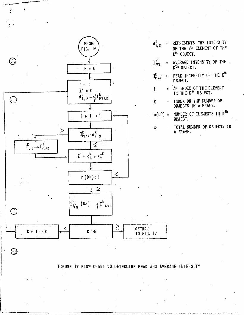
-FRm~ K

d· 3 : FIG. 16

I, = REPRESEIITS THE I ~ITEnS IlY

OF THE jth ELEMENT OF THE J<th OBJECT.

@ K . j',;~,>~ lAVE

K = 0 = AVERAGE HlTENS IlY OF TH E .

Kth OBJECT.

~ ~EAK' i = I

= PEAK I tlTEUS IlY OF, THE Kth OBJECT.

rK = 0 i k .. --' ik

0 dl,3~IPEAK K

= AN INDEX OF THE ELEMENT IN THE Kth OBJECT.

= ItWEX ON THE Nut~BER OF

~ ,

"

OBJECTS I N A FRA~lE.

i + I-+i n(DK) = tlUMBER OF ELEMEtlTS IN Kih OBJECT.

1 <l> > K K i IpEAK:d i, 3

= TOTAL NUMBER OF OBJECTS IN A FRAME.

K K J< . d i, 3 --.-IpEAK

.

I K K f I + di,3~

~ n(OK):i <

~

. 'l ~ k

(Dk) irk AVE r., 0 ' n

~ < > RETURN '- K + I--K .~ K:<l> -

TO FI G. 12

FIGURE 17 FLOW CHART TO. DETERMINE PEAK AND ,AVERAGE-INTENSITY

.' ,

!

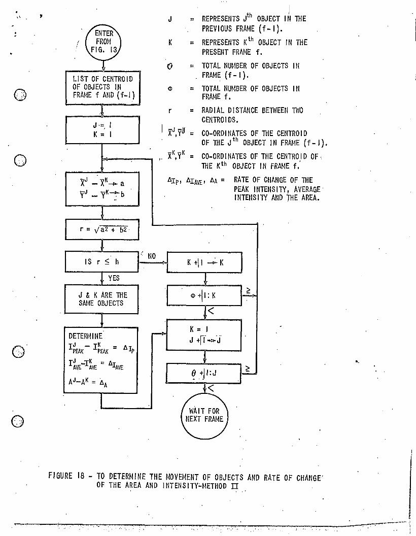
0 .' It\.

0 " .

G , '

0 . ,

I J = REPRESENTS Jth OBJECT I N TIlE

ENTER PREVIOUS FRAME (f - I).

REPRESENTS K th 0 ! FROM K = BJECT IN THE FIG. 13 PRESENT FRAME f.

<9 = TOTAL Nut.1BER OF OBJECTS III

LI ST OF CENTRO I D . FRAME (f - I).

OF OBJECTS I.N ct> = TOTAL NU~mER OF OBJECTS I tI FRM·1E f AND (f-I ) FRAME f •

.1 r = RADIAL DISTANCE BElWEEU TWO

J.=, I CENTROI DS.

I -J -8 CO-ORDINATES OF TIlE CENTRO I D K = I X ,Y = OF TIlE J th OBJE CT J N FRAt·1E (f - I ) •

}(K -K CO-ORDINATES OF TUE CENTRO I D OF. ,,, ,Y = , TIlE Kth OBJECT I N FRA~1E f.

-J 'XK Alp, AIAYE' AA = RATE OF CHAtiGE OF TIlE X - --Jb- a PEAK IN TENSITY, AVERAGE' V" _ yK~b ItITEtlS I TY AND THE AREA. -

r = va2 + b2·

~ IS r $ h

( NO K +\1 ~ I<

YES ! ct> +11 : K

> J & K ARE lliE i--=-> SAt~E OBJ ECTS

!< K = I

~ DETERI~INE J {f~"j" IJ - IK = AIp PEAK PEAK

~ rJ _rK = AI AVE AVE AVE

~ +) I:J > ~

AJ-AK = AA ~

( WAIT FOR ) NEXT FRAME

I -

FI GURE 18 - TO DETERM I tlE THE t~OYEMENT OF OBJECTS AND RATE OF CHANGE" OF THE AREA AND I NTEtiS ITY~HETHOD 11

".

;' ,

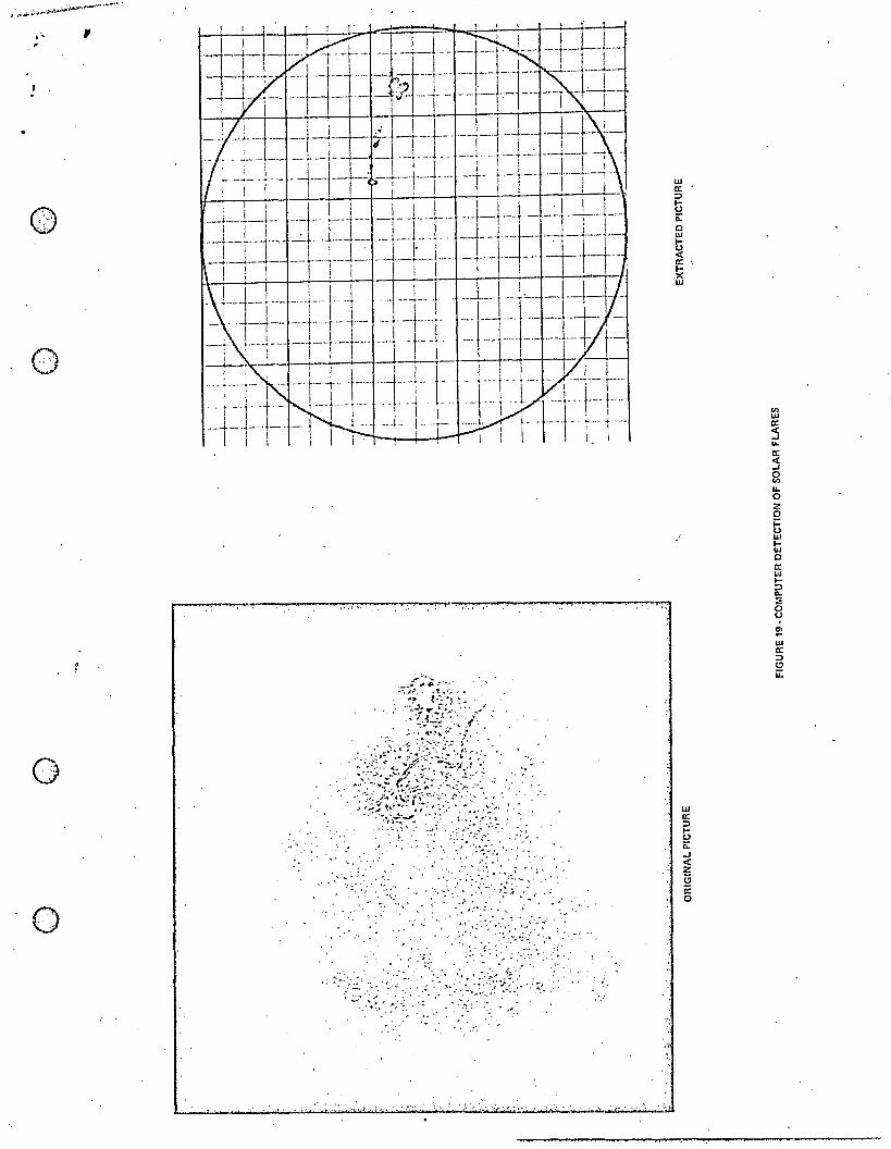
o

o

'0" .'

. ..,-~~~----~'_I~" • ~ft;",j4~ , ' ' . "',r',' i; • 1 ,. 4\f! •

-- -

... ;"~"""

- . "

.,\ ~.

'" -. ~ ,:

" . ,'-'~. ~ ; ~'

. . ....,' .' .,:L; ;d::: .... .' .... ;:":~;~;,;:,',:' .

': ~~>: - . .. : .. ;-.~.:.' . ,Y..t·;·:: ,<.: .. ~ ..

': c>.::~~.:~~:.::.·:.~:~~ .. ~~·:'{;~:_:AY·~~~:~-:;::· ,'. '" ~ .J'

\.,',,,,' I, '."'.,'" '

. , .. ,

w a:

t ii: c w

~ a:1

E

II> W

~ oJ LL

a: :J g LL o Z o ~ w tu c a: w ~ ~ "~ o Co)

"

, , 0,

()

, ~t

( ..

,', '" ", .. f-.... · " .. ' "°"1" ...... ;y I ... ' .,' •. '.' ...... .

-.

.~

w CC

~ c: o w

~ CC

S

w cc :> t; c: ..J <t: z c; a: o

!3 CC

S "a: S g "o 2: o ti w Iii o a: w

5 .... ::;: 8 ~ w cc :> Cl u::

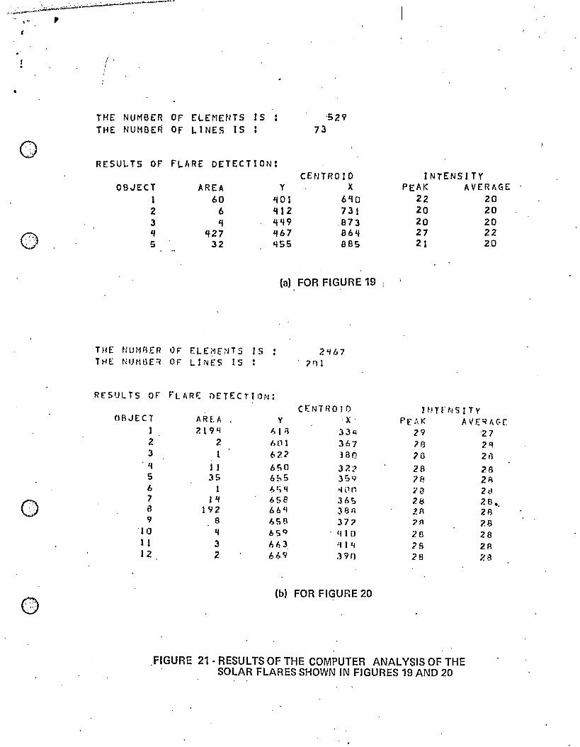
t

•

Q

0·', " . '.I

0 ~ -,'

0 <,"

I . r

THE NUMBER or ELEMENTS IS THE NUMBER OF LINES IS

RESULTS or FLARE DETECTION:

OBJECT AREA Y 1 60 'f01 2 6 'f12 3 'f 'f'f9 'f , ... 27 'f67 S 32 'iSS

529 73

CENTROID X

6ttO 731

,873 86q BSS

(a) FOR FIGURE 19

THE NUMBER 0F ELEMOJT5 IS 2'167 THE NUMoE1 OF" LINES I S "Ill

RES'.)L r5 OF FLARF.: nETECTIOf.J: CfNTHOl1)

ORJECT AREA Y ,X'

1 7.19LJ ~1i3 3311 2 2 hOI )67 3 1 622 )80

''1 J 1 b~O 37.<, 5 35 6SS -,\Sr.;>

6 1 6'; if of ('11

7 J '* 658 36; 8 192 bbif 38A 9 a /:,s~ 37-;

'10 'I 65 Q ' lj 1 ()

1 1 3 ,.,,, 3, "f 1 tj 12 2 bb9 .)9f)

(b) FOR FIGUBE 20

INTENSITY PEAK AVERAGE

22 20 20 20 20 20 27 22 21 20

I ~! T F to] 5 I T y p r..\ K AVF:.~f,r-[

29 '27 70 2q 70 211

28 28 78 2A 2~ 2d 28 28., .?A 2A ;>A 7.8 28 28 ;>5 2R 28 28

FIGURE 21 • RESULTS OF THE COMPUTER ANALYSIS OF THE SOLAR FLARES SHOWN IN FIGURES 19 AND 20

0 ..

:E en 0 ex: 0 ~ UJ Cl c:x: ex: 0 .... (/)

c:x:

~ '0 LL. 0 ex: UJ OJ :E ::> z

o ' .

0,

, " :

104

103

- SQUARE FLARE CONFIGURATION

--- RECTANGULAR FLARE CONFIGURATION (5 ELEMENTS PER LINE)

102 ~ __ ~ __ ~ __ ~~ __ ~ __ ~ __ ~ ____ L-__ ~ __ ~ ____ ~ __ ~ __ ~ __ ~~~

1 2 3 4 5 6 7. 8 9 10 11 12 13 14 15

NUMBER OF FLARES/FRAME

FIGURE 22 . DATA STORAGE REQUIREMENTS·METHOD \I

I i

I I !

i J

'I '1 I

! I :

)rib C;-!/J!7.3' NO:m~ · TlTLE-Automatic Spaceborne Solar Flare ... Bell Telephone Laboratories....

Documents

Transcript of )rib C;-!/J!7.3' NO:m~ · TlTLE-Automatic Spaceborne Solar Flare ... Bell Telephone Laboratories....