Rheology and structure of ceramic suspensions under · PDF fileij Di usion tensor used in...
120
UNIVERSIT ´ E DE LIMOGES ´ Ecole Doctorale Sciences et Ing´ eniere en Mat´ eriaux, M´ ecanique Energ´ etique et A´ eronautique Facult´ e des Sciences et Techniques Laboratoire de Science des Proc´ ed´ es C´ eramique et de Traitements de Surface UNIVERSITA DEGLI STUDI DI GENOVA Scuola di Dottorato Scienze e Tecnologie per l’Informazione e la Conoscenza (XXVI ciclo) Dipartimento Di Fisica Thesis [XX/2015] Dissertation under joint supervision with European Doctorate Certificate of the requirements for the degrees of: DOCTEUR DE L’UNIVERSIT ´ E DE LIMOGES Sp´ ecialit´ e: Mat´ eriaux C´ eramiques et Traitements de Surface and DOTTORE DI RICERCA IN FISICA della Scuola di Dottorato Scienze e Tecnologie per l’Informazione e la Conoscenza (XXVI ciclo) presented and defended by Aleena Maria LAGANAPAN November 26, 2015 Rheology and structure of ceramic suspensions under constraints: a computational study Thesis supervisors: Arnaud Videcoq, Riccardo Ferrando and Marguerite Bienia COMMITTEE : Tapio ALA-NISSILA Professor, Aalto University Reviewer Paul BOWEN Professor, ´ Ecole Polytechnique F´ ed´ erale de Lausanne Reviewer Christophe MARTIN Directeur de Recherche CNRS (HDR), Universit´ e de Grenoble Alpes Examiner Riccardo FERRANDO Professor, Universita degli Studi di Genova Examiner Arnaud VIDECOQ Maˆ ıtre de Conf´ erence (HDR), SPCTS Examiner Marguerite BIENIA Maˆ ıtre de Conf´ erence, SPCTS Examiner
-
Upload
nguyenlien -
Category
Documents
-
view
223 -
download
3
Transcript of Rheology and structure of ceramic suspensions under · PDF fileij Di usion tensor used in...
UNIVERSITE DE LIMOGES
Ecole Doctorale
Sciences et Ingeniere en Materiaux,
Mecanique Energetique et Aeronautique
Faculte des Sciences et Techniques
Laboratoire de Science des Procedes
Ceramique et de Traitements de Surface
UNIVERSITA DEGLI STUDI
DI GENOVA
Scuola di Dottorato
Scienze e Tecnologie
per l’Informazione e la Conoscenza
(XXVI ciclo)
Dipartimento Di Fisica
Thesis [XX/2015]
Dissertation under joint supervision with European DoctorateCertificate of the requirements for the degrees of:
DOCTEUR DE L’UNIVERSITE DE LIMOGES
Specialite: Materiaux Ceramiques et Traitements de Surface
and
DOTTORE DI RICERCA IN FISICA
della Scuola di Dottorato Scienze e Tecnologie per l’Informazione e laConoscenza (XXVI ciclo)
presented and defended by
Aleena Maria LAGANAPAN
November 26, 2015
Rheology and structure of ceramicsuspensions under constraints: a
computational study
Thesis supervisors:
Arnaud Videcoq, Riccardo Ferrando and Marguerite Bienia
COMMITTEE :
Tapio ALA-NISSILA Professor, Aalto University Reviewer
Paul BOWEN Professor, Ecole Polytechnique Federale de Lausanne ReviewerChristophe MARTIN Directeur de Recherche CNRS (HDR), Universite de Grenoble Alpes ExaminerRiccardo FERRANDO Professor, Universita degli Studi di Genova ExaminerArnaud VIDECOQ Maıtre de Conference (HDR), SPCTS ExaminerMarguerite BIENIA Maıtre de Conference, SPCTS Examiner


Table of contents
Contents
Rheology and structure of ceramic suspensions under constraints Page 1

Table of contents
Nomenclature . . . . . . . . . . . . . . . . . . . . . . . . . . . . . . . . . 4
List of figures . . . . . . . . . . . . . . . . . . . . . . . . . . . . . . . . . 10
List of tables . . . . . . . . . . . . . . . . . . . . . . . . . . . . . . . . . . 13
Summary . . . . . . . . . . . . . . . . . . . . . . . . . . . . . . . . . . . 15
Resume . . . . . . . . . . . . . . . . . . . . . . . . . . . . . . . . . . . . 17
Riassunto . . . . . . . . . . . . . . . . . . . . . . . . . . . . . . . . . . . 20
Introduction . . . . . . . . . . . . . . . . . . . . . . . . . . . . . . . . 22
Chapter 1 : Simulation Techniques . . . . . . . . . . . . . 271.1 Scale separation . . . . . . . . . . . . . . . . . . . . . . . . . . . . . . . . . 281.2 Molecular Dynamics . . . . . . . . . . . . . . . . . . . . . . . . . . . . . . 301.3 Brownian Dynamics . . . . . . . . . . . . . . . . . . . . . . . . . . . . . . . 311.4 Other Mesoscale Methods . . . . . . . . . . . . . . . . . . . . . . . . . . . 33
1.4.1 Dissipative Particle Dynamics . . . . . . . . . . . . . . . . . . . . . 331.4.2 Lattice-Boltzmann . . . . . . . . . . . . . . . . . . . . . . . . . . . 33
1.5 Stochastic Rotation Dynamics . . . . . . . . . . . . . . . . . . . . . . . . . 341.5.1 Sheared SRD fluid . . . . . . . . . . . . . . . . . . . . . . . . . . . 361.5.2 Thermostats . . . . . . . . . . . . . . . . . . . . . . . . . . . . . . . 39
1.5.2.1 Simple Scaling Thermostat . . . . . . . . . . . . . . . . . 401.5.2.2 Monte-Carlo Thermostat . . . . . . . . . . . . . . . . . . . 40
1.5.3 Coupling SRD with MD . . . . . . . . . . . . . . . . . . . . . . . . 411.6 Mapping between physical and SRD-MD time scales . . . . . . . . . . . . . 441.7 Summary . . . . . . . . . . . . . . . . . . . . . . . . . . . . . . . . . . . . 46
Chapter 2 : Shear Viscosity . . . . . . . . . . . . . . . . . . . 482.1 System . . . . . . . . . . . . . . . . . . . . . . . . . . . . . . . . . . . . . . 492.2 Shear viscosity of pure fluids . . . . . . . . . . . . . . . . . . . . . . . . . . 51
2.2.1 Equilibrium approach . . . . . . . . . . . . . . . . . . . . . . . . . . 512.2.2 Non-equilibrium approach . . . . . . . . . . . . . . . . . . . . . . . 522.2.3 Winkler’s formulation . . . . . . . . . . . . . . . . . . . . . . . . . 54
2.2.3.1 Equilibrium case . . . . . . . . . . . . . . . . . . . . . . . 542.2.3.2 Non-equilibrium case . . . . . . . . . . . . . . . . . . . . . 56
2.3 Embedded colloids . . . . . . . . . . . . . . . . . . . . . . . . . . . . . . . 582.3.1 Analytical method . . . . . . . . . . . . . . . . . . . . . . . . . . . 582.3.2 Numerical method . . . . . . . . . . . . . . . . . . . . . . . . . . . 592.3.3 Stress Tensors . . . . . . . . . . . . . . . . . . . . . . . . . . . . . . 61
2.4 Shear Viscosity . . . . . . . . . . . . . . . . . . . . . . . . . . . . . . . . . 622.5 Conclusions . . . . . . . . . . . . . . . . . . . . . . . . . . . . . . . . . . . 66
Rheology and structure of ceramic suspensions under constraints Page 2

Table of contents
Chapter 3 : Percolation threshold . . . . . . . . . . . . . 683.1 Yield stress model . . . . . . . . . . . . . . . . . . . . . . . . . . . . . . . . 703.2 On hydrodynamic effects . . . . . . . . . . . . . . . . . . . . . . . . . . . . 713.3 Mapping from physical values to simulation parameters . . . . . . . . . . . 723.4 Time scales . . . . . . . . . . . . . . . . . . . . . . . . . . . . . . . . . . . 743.5 Parameters for aggregate analysis . . . . . . . . . . . . . . . . . . . . . . . 75
3.5.1 Number of aggregates vs time (NA vs t) . . . . . . . . . . . . . . . 753.5.2 Parameters PD and φc . . . . . . . . . . . . . . . . . . . . . . . . . 763.5.3 Number of nearest neighbors . . . . . . . . . . . . . . . . . . . . . . 77
3.6 Results . . . . . . . . . . . . . . . . . . . . . . . . . . . . . . . . . . . . . . 773.6.1 Dissociation times . . . . . . . . . . . . . . . . . . . . . . . . . . . . 773.6.2 Influence of the colloid-colloid attraction strength . . . . . . . . . . 783.6.3 Influence of HIs . . . . . . . . . . . . . . . . . . . . . . . . . . . . . 813.6.4 Percolation threshold measurements . . . . . . . . . . . . . . . . . . 82
3.7 Conclusions . . . . . . . . . . . . . . . . . . . . . . . . . . . . . . . . . . . 84
Chapter 4 : Attractive Walls and Shaking . . . . . . 864.1 Attractive Walls . . . . . . . . . . . . . . . . . . . . . . . . . . . . . . . . . 874.2 System: suspension with attractive walls . . . . . . . . . . . . . . . . . . . 884.3 Parameters for Aggregate Analysis . . . . . . . . . . . . . . . . . . . . . . 924.4 Results . . . . . . . . . . . . . . . . . . . . . . . . . . . . . . . . . . . . . . 92
4.4.1 NaCl vs CsCl . . . . . . . . . . . . . . . . . . . . . . . . . . . . . . 924.4.2 Strength of the wall (εWall) vs. inverse range of interaction (κa) . . . 944.4.3 CsCl formation starts from the wall . . . . . . . . . . . . . . . . . . 954.4.4 Number of colloids per layer and interaction energy with the wall . 97
4.5 Shaken Aggregates . . . . . . . . . . . . . . . . . . . . . . . . . . . . . . . 994.6 System: Modeling oscillatory flows . . . . . . . . . . . . . . . . . . . . . . 1014.7 Results for Shaken Aggregates . . . . . . . . . . . . . . . . . . . . . . . . . 1024.8 Conclusions . . . . . . . . . . . . . . . . . . . . . . . . . . . . . . . . . . . 104
Conclusions . . . . . . . . . . . . . . . . . . . . . . . . . . . . . . . . . 106
Bibliography . . . . . . . . . . . . . . . . . . . . . . . . . . . . . . . . . . . 109
Rheology and structure of ceramic suspensions under constraints Page 3

Nomenclature
Rheology and structure of ceramic suspensions under constraints Page 4

Nomenclature
Nomenclature
Rheology and structure of ceramic suspensions under constraints Page 5

Nomenclature
α Rotation angle
∆tBD Time step for BD simulations
∆tLB Time step for LB simulations
∆tMD Time step for MD simulations
∆tSRD Time step for SRD simulations
∆vy Shear velocity
δij Kronecker delta.
γ Shear rate
εWall Interaction parameter for LJ 9-3 potential
εwall Interaction parameter between the wall and the fluid particles
εcc Interaction parameter between the colloids
εcf Interaction parameter between the colloids and the fluid
η Viscosity of water (10−3 Pa · s)
γ Average number of fluid particles in each cell
rij Unit vector in the direction of rij
λ Dimensionless mean free path
T Instantaneous temperature
ν Kinematic viscosity
φc Percolation threshold
φmax Maximum packing fraction
ρf Mass density of the SRD fluid
σWall Interaction parameter for LJ 9-3 potential
σwall Interaction parameter between the wall and the fluid particles
σcc Interaction potential between the colloids
σcf Interaction potential between the colloids and the fluid
τ Yield stress
τB Brownian relaxation time
τD Colloid diffusion time
Rheology and structure of ceramic suspensions under constraints Page 6

Nomenclature
τf Fluid relaxation time
τν Kinematic time
τFP Fokker-Planck time
εWall Attraction strength between the colloids and the wall
ς Strength of stochastic forces in DPD simulations
ζ Friction coefficient of the solvent
ζE Enskog friction coefficient
ζS Stokes friction coefficient
A Acceptance probability in the Monte-Carlo thermostat
a Colloid radius
a0 cell size
Bij Parameter for the hard-wall potential
c Thermostat strength
Cij Parameter for the hard-wall potential
D0 Diffusion coefficient of an isolated colloid
DSRD Diffusion coefficient in the SRD simulations
Dij Parameter for the hard-wall potential
I Identity tensor
kB Boltzmann constant
L Side length of the simulation box
l Dimension of the simulation box in terms of the number of cells
M Mass of the colloid
m1 Yield stress factor
NA Number of aggregates
Nc Number of embedded colloids
Nf Number of fluid particles in a simulation box
ni(r, t) Represents the fluid density in LB simulations
neqi (r, t) Represents the equilibrium value of the fluid density in LB simulations
Rheology and structure of ceramic suspensions under constraints Page 7

Nomenclature
P2D Structural parameter that determines between NaCl and CsCl lattice types
P3D Structural parameter that determines between NaCl and CsCl lattice types
rcc Cut-off radius in the colloid-colloid interaction
rcf Cut-off radius in the colloid-fluid interactions
S Thermostat scaling factor
T Average temperature of the system
T0 Reference temperature
TSRD Average temperature of the system in SRD simulations
tSRD SRD time scale
UWall Potential describing the attractive wall
Ucc Interaction potential between the colloids
Ucf Interaction potential between the colloids and the fluid
UHWij Hard-wall potential
V Volume of the simulation box
Vf Free volume accessible to the fluid particles inside the simulation box
Vwf Interaction potential between the wall and the fluid particles
Yi Uncorrelated Gaussian variables used in BD simulations.
Z Colloid charge
Γi(t) Represents the random forces received by the colloids from the fluid in a BDsimulation
Ξi(t) Represents the frictional forces in a BD simulation
ai Acceleration of the ith particle
ci Represents the velocity of the lattice sites in LB simulations
Dij Diffusion tensor used in BD-YRP
Fcij Represents interparticle forces in DPD simulations
Fdij Represents the velocity-dependent forces in DPD simulations
Ffij Represents the stochastic forces in DPD simulations
Fi Total force between particles i and j
R Rotation matrix
Rheology and structure of ceramic suspensions under constraints Page 8

Nomenclature
ri Position of the ith particle
vi Velocity of the ith particle
vcm Center of mass velocity inside the simulation box
Uij Interaction potential between particles i and j
HIs Hydrodynamic interactions
IP Inverse power potential
LEBC Lees Edwards boundary conditions
Rheology and structure of ceramic suspensions under constraints Page 9

List of figures
List of Figures
Rheology and structure of ceramic suspensions under constraints Page 10

List of figures
1.1 Schematic Diagram of a 2-D SRD system . . . . . . . . . . . . . . . . . . . 361.2 Schematic diagram of Lees-Edwards boundary conditions implementation . 381.3 Thermostat strength (c) vs Temperature . . . . . . . . . . . . . . . . . . . 411.4 The two kinds of SRD-MD coupling . . . . . . . . . . . . . . . . . . . . . . 432.1 Shear viscosity of pure fluid using Winkler’s approach . . . . . . . . . . . . 572.2 Time evolution of velocity profile . . . . . . . . . . . . . . . . . . . . . . . 592.3 Shear Viscosity vs. σcf . . . . . . . . . . . . . . . . . . . . . . . . . . . . . 602.4 Sample stress tensor for
mf
Vv′iyvix component . . . . . . . . . . . . . . . . . 63
2.5 Sample stress tensor for Mc
Vv′iyvix component . . . . . . . . . . . . . . . . . 63
2.6 Shear viscosity contribution from colloids . . . . . . . . . . . . . . . . . . . 642.7 Shear viscosity contribution from the SRD fluid . . . . . . . . . . . . . . . 642.8 Suspension’s shear viscosity vs. volume fraction . . . . . . . . . . . . . . . 653.1 Schematic diagram of percolating and non-percolating 2D clusters . . . . . 693.2 DLVO potential . . . . . . . . . . . . . . . . . . . . . . . . . . . . . . . . . 743.3 Schematic diagram of nearest neighbors . . . . . . . . . . . . . . . . . . . . 763.4 Degree of ordering: Diffusion time scale vs. Dissociation time scale . . . . 783.5 NA vs t for the percolation study . . . . . . . . . . . . . . . . . . . . . . . 793.6 PD vs. φ for systems without HIs . . . . . . . . . . . . . . . . . . . . . . . 803.7 PD vs. φ for sytems with and without HIs . . . . . . . . . . . . . . . . . . 813.8 Sample aggregate shapes when HIs are absent/present . . . . . . . . . . . . 823.9 Order parameter for sytems with 5kBT potential well . . . . . . . . . . . . 833.10 Summary: Phase space diagram for percolation threshold . . . . . . . . . . 844.1 NaCl and CsCl primitive cells . . . . . . . . . . . . . . . . . . . . . . . . . 874.2 Schematic diagram of the walled system . . . . . . . . . . . . . . . . . . . 894.3 Yukawa potential . . . . . . . . . . . . . . . . . . . . . . . . . . . . . . . . 914.4 Snapshots for NaCl → CsCl lattice transformation . . . . . . . . . . . . . . 934.5 P3D measurement for κa = 2.55 and U0 = 9kBT . . . . . . . . . . . . . . . 944.6 P3D plot used to determine CsCl seeding . . . . . . . . . . . . . . . . . . . 964.7 CsCl component of P3D . . . . . . . . . . . . . . . . . . . . . . . . . . . . . 964.8 CsCl (101) plane vs. NaCl (100) plane . . . . . . . . . . . . . . . . . . . . 974.9 P2D parameter for the system with κa = 1.5. . . . . . . . . . . . . . . . . . 984.10 Number of colloids vs. the distance from the wall . . . . . . . . . . . . . . 994.11 The influence of L on the parameter P3D . . . . . . . . . . . . . . . . . . . 1004.12 Total energies of NaCl vs. CsCl structures . . . . . . . . . . . . . . . . . . 1004.13 Odering of an equilibrium suspension vs. shaken suspensions . . . . . . . . 1024.14 Ordering of shaken suspensions vs. BD equilibrium suspensions . . . . . . 1034.15 NA vs. t for shaken suspensions . . . . . . . . . . . . . . . . . . . . . . . . 103
Rheology and structure of ceramic suspensions under constraints Page 11

List of figures
Rheology and structure of ceramic suspensions under constraints Page 12

List of tables
List of Tables
Rheology and structure of ceramic suspensions under constraints Page 13

List of tables
1.1 Hierarchy of time scales . . . . . . . . . . . . . . . . . . . . . . . . . . . . 301.2 Summary of mesoscopic simulation techniques . . . . . . . . . . . . . . . . 472.1 SRD parameters for the shear viscosity of pure fluids . . . . . . . . . . . . 502.2 Corresponding Nc and Nf values for every φ . . . . . . . . . . . . . . . . . 603.1 Corresponding Nf values for every φ . . . . . . . . . . . . . . . . . . . . . 723.2 Parameters for the percolation study . . . . . . . . . . . . . . . . . . . . . 733.3 Hierarchy of time scales for the percolation study . . . . . . . . . . . . . . 753.4 SRD parameters used in the study of percolation threshold. . . . . . . . . 753.5 Dissociation times for BD and SRD-MD. . . . . . . . . . . . . . . . . . . . 784.1 Parameters for system with attractive walls . . . . . . . . . . . . . . . . . 894.2 εWall (kBT ) and εWall(kBT ) . . . . . . . . . . . . . . . . . . . . . . . . . . . 914.3 Structures formed for κa = 2.55, 3 . . . . . . . . . . . . . . . . . . . . . . 934.4 Structures formed for κa = 1.5 . . . . . . . . . . . . . . . . . . . . . . . . . 954.5 Number of colloids in the first layer . . . . . . . . . . . . . . . . . . . . . . 98
Rheology and structure of ceramic suspensions under constraints Page 14

Summary
Summary
The numerical study of colloidal suspensions is an integral part of several ceramic
and biological processes. The main challenge of this thesis is to understand and predict
the structural and rheological behaviours of the colloids when complexities such as (1)
hydrodynamic interactions (HIs) and (2) external forces are incorporated in the system.
These factors are difficult to model because of the disparity in size between the colloids
and the fluid particles. Hence there is a clear separation of length and time scales between
the physics of the colloids and the fluid.
A convenient way to address this problem is to average-out the effects of the fluid so
that the modeling of the colloidal suspension is more maneagable. In this regard, this
thesis employs two of the fastest numerical techniques available in literature: standard
Brownian Dynamics (BD), for systems where HIs can be ignored; and hybrid Stochastic
Rotation Dynamics - Molecular Dynamics (SRD-MD), for systems where HIs need to
be incorporated. The two types of external forces explored in this thesis are shear and
attractive walls. Suspensions under shear are simulated using SRD-MD, while the system
with attractive walls is simulated using BD. BD and SRD-MD are also simultaneously
applied when the effects of HIs need to be isolated and analyzed.
We study three different systems of colloidal suspensions. The first is a system of
hard spheres under shear, where we verify that the modeling of HIs in SRD-MD can
accurately reproduce the relation between shear viscosity and volume fraction. Since
SRD-MD is a relatively recent technique, its potential as a simulation method is not
yet fully-explored. We develop SRD-MD by incorporating shear, with a Monte-Carlo
thermostat, in MD-coupled sytems. From this model, we can apply the non-equilibrium
approach for the calculation of shear and derive a stress tensor for dilute and concentrated
systems. The shear viscosity results are in agreement with known analytical, numerical
and experimental data. We also show that the shear viscosity of the suspension can
be divided into components: one is shear viscosity contributions from the fluid and
colloid components; and the other is shear viscosity contributions from the streaming
and collisional components. Hence our method of calculation allows for a more in-depth
characterization of the viscosity of the suspension. In this study, we establish that SRD-
MD fully captures the required hydrodynamic effects in sheared suspensions thus making
SRD-MD a valuable tool for modeling an interesting range of systems under shear.
The second system consists of aqueaous alumina suspensions described by the
Derjaguin-Landau-Verwey-Overbeek (DLVO) potential. We analyze the percolation
behaviour of the system by employing BD and SRD-MD methods. The percolation
phenomenon is characterized by the formation of an infinite network of colloidal aggregates
that spans through space. The parameters that influence the percolation threshold (φc)
Rheology and structure of ceramic suspensions under constraints Page 15

Summary
are colloid-colloid attraction strength and HIs. The simulations show that φc decreases
with increasing colloid-colloid attraction strength since this can lead to more elongated
structures. Moreover, we observe that systems with HIs tend to have more elongated
structures during the aggregation process than systems without HIs. This results to a
sizable decrease in φc when the colloid-colloid attraction is not too strong. On the other
hand, the effects of HIs tend to become negligible with increasing attraction strength. Our
φc values are in good agreement with those estimated by the yield stress model (YODEL)
by Flatt and Bowen. This work can be useful, alongside YODEL, in predicting the yield
stress magnitude of ceramic materials.
The third sytem consists of binary colloids described by a Yukawa potential. The
binary system is placed under the influence of an attractive wall that is described by
a Lennard Jones 9-3 potential. We evolve the system using BD and demonstrate that
the presence of an attractive wall can modify the expected equilibrium structures of the
colloids. In particular, the attractive wall can alter the lattice structure of the aggregates
on the surface such that CsCl-type lattices are formed instead of metastable NaCl-type
lattices. We also examine the parameters that lead to this kind of lattice transformation:
the colloid-wall attraction strength (εWall), the colloid-colloid attraction strength (U0),
and the inverse range of interaction (κa). The variables κ and a denote the inverse of
Debye screening length and the radius of the colloids respectively, and the values of κa
are restricted in the following range: κa ∈ [1, 3]. The results show that the probability of
obtaining a CsCl structure increases when the force of attraction from the wall exceeds
the inter-colloid attraction (εWall > U0). In addition to this, the likelihood of obtaining
CsCl increases and when κa is relatively small (longer range of repulsion). Consequently,
for systems with εWall < U0, the aggregates tend to remain as NaCl. The reason why
CsCl structure is more favored is because it has a more compact formation at the surface.
Moreover, the total energy, between the colloidal structure and the surface, is smaller in
the CsCl-cases than in the NaCl-cases. This study can have implications on researches
that invlove surface-grown ceramics and protein adsorption.
Finally, we perform preliminary investigations on shaken suspensions by SRD-MD. The
system is the same as the percolating alumina system described above. The difference
is that the colloidal suspension is now placed under an oscillating shear with a shear
rate of 10 s−1 and a frequency of 20 s−1. We demonstrate that when the oscillating
motion of the suspension occurs simultaneously with the aggregation process of the
colloids, more compact structures are formed. Moreover, it seems that the suspensions
undergoing oscillatory motion reorganize at a faster rate than suspensions in equilibrium.
This technique of agitating the suspensions can be used to artificially manipulate the
dissociation and association rates of the colloids thus promoting more ordered structures.
Rheology and structure of ceramic suspensions under constraints Page 16

Summary - Resume
Resume
L’etude numerique des suspensions colloıdales fait partie integrante de differents
procedes ceramiques et biologiques. L’enjeu principal de cette these est de comprendre
et predire les proprietes structurales et rheologiques de suspensions colloıdales en tenant
compte d’elements complexes tels que (1) les interactions hydrodynamiques (IHs) et/ou
(2) des forces exterieures. La simulation numerique d’une suspension colloıdale est difficile
du fait des tailles tres differentes des colloıdes et des molecules de liquide. Il y a par
consequent une separation importante entre les echelles de longueur et de temps associees
a la physique des colloıdes et a la physique du fluide.
Un moyen de parvenir a simuler une suspension colloıdale est de moyenner les effets
du fluide. De ce point de vue, nous employons dans cette these deux des techniques
numeriques les plus rapides de la litterature: la dynamique brownienne standart (BD),
pour les systemes ou les IHs peuvent etre ignorees; et la technique hybride ”stochastic
rotatoin dynamics - molecular dynamics” (SRD-MD), pour les systemes ou les IHs doivent
etre incorporees. Les deux types de forces exterieures explorees dans cette these sont le
cisaillement et la presence d’un mur attractif. Les suspensions soumises au cisaillement
sont simulees par SRD-MD, alors que le systeme avec le mur attractif est simule par BD.
BD et SRD-MD sont aussi employees simultanement lorsqu’il s’agit d’isoler et d’analyser
les effets des IHs.
Trois systemes colloıdaux differents ont ete etudies. Le premier est un systeme de
spheres dures soumis a un cisaillement, ou le but a ete de verifier que l’introduction des
IHs dans la SRD-MD peut correctement reproduire la relation entre la viscosite et la
fraction volumique. Du fait que la SRD-MD est une technique relativement recente, son
potentiel en tant que methode de simulation n’est pas encore totalement explore. Nous
avons developpe la SRD-MD en incorporant le cisaillement, avec un thermostat Monte-
Carlo. Nous avons applique l’approche hors equilibre pour le calcul du cisaillement et
derive un tenseur des contraintes pour les systemes dilues et concentres. Les resultats de
viscosite sont en accord avec les resultats connus, qu’ils soient analytiques, numeriques
et experimentaux. Nous montrons egalement que la viscosite de la suspension peut-
etre decomposee en differentes contributions: celles du fluide et des colloıdes; puis celles
des etapes d’ecoulement et des collisions. Cette etude permet donc une caracterisation
detaillee de la viscosite des suspensions, ou nous montrons que la SRD-MD decrit bien les
effets hydrodynamiques dans les suspensions cisaillees, ce qui en fait un outil interessant
pour simuler les systemes sous cisaillement.
Le second systeme consiste en une suspension d’alumine, pour laquelle les interactions
sont decrites par la theorie DLVO (Derjaguin-Landau-Verwey-Overbeek). Une etude de la
percolation a ete realisee par les methodes BD et SRD-MD. La percolation est caracterisee
Rheology and structure of ceramic suspensions under constraints Page 17
Summary - Resume
par la formation d’un reseau d’agregats qui traverse la boıte de simulation d’un bout a
l’autre. Les parametres dont nous avons etudie les effets sur le seuil de percolation (φc)
sont la profondeur du puits de potentiel caracterisant l’attraction entre les colloıdes et les
IHs. Les simulations montrent que φc diminue lorsque la profondeur du puits de potentiel
augmente, car les agregats formes sont plus allongees. De plus, nous observons que la prise
en compte des IHs tend a former des structures plus allongees egalement, par rapport aux
structures obtenues sans les IHs. Ceci se traduit par une diminution de φc lorsque le
puits de potentiel n’est pas trop profond. D’autre part, l’effet des IHs devient negligeable
lorsque la profondeur du puits de potentiel augmente. Les valeurs de φc obtenues dans les
simulations sont en bon accord avec celles estimees par le modele de la contrainte seuil
(YODEL) etabli par Flatt et Bowen. Ce travail peut etre utile, de facon complementaire
a YODEL, pour predire la contrainte seuil de suspensions ceramiques.
Le troisieme systeme comporte deux types de colloıdes qui interagissent par un
potentiel de Yukawa. Ce systeme binaire est soumis a l’influence d’un mur attractif
dont l’interaction avec les colloıdes est decrite par un potentiel de Lennard-Jones 9-3.
L’agregation des colloıdes dans ce systeme est simulee par BD et nous montrons que
la presence d’un mur attractif peut modifier les structures d’equilibre attendues. En
particulier, le mur attractif peut alterer la structure cristalline des agregats a la surface
telle qu’une structure de type CsCl qui se forme au lieu de la structure metastable de
type NaCl. Nous avons etudie les parametres qui conduisent a ce type de changement de
configuration: la profondeur du puits de potentiel colloıde-mur (εWall), celle du puits de
potentiel colloıde-colloıde (U0), et l’inverse de la portee des interactions colloıde-colloıde
(κa). Les variables κ et a sont respectivement l’inverse de la longueur d’ecrantage de
Debye et le rayon des colloıdes. Le domaine de variation de κa etudie ici est: κa ∈ [1, 3].
Les resultats montrent que la probabilite d’obtenir une structure CsCl augmente quand
l’attraction colloıde-mur excede l’attraction colloıde-colloıde (εWall > U0). De plus, la
tendance a la formation de la structure CsCl augmente lorsque κa est relativement faible
(interactions colloıde-colloıde de plus longue portee). En consequence, pour les systemes
ou εWall < U0, les agregats tendent a rester dans la structure NaCl. La raison pour laquelle
la structure CsCl est plus favorable vient du fait qu’elle est plus compacte a la surface.
L’energie totale, entre la structure colloıdale et la surface est plus faible dans le cas d’une
structure CsCl que dans le cas d’une structure NaCl. Cette etude montre l’importance
des interactions avec les parois environnantes sur les structures colloıdales qui peuvent se
former.
Finalement, nous avons realise une etude preliminaire par SRD-MD de suspensions
soumises a un cisaillement oscillant. Le systeme est le meme que celui de l’etude sur la
percolation. Le taux de cisaillement est de 10 s−1 et la frequence de 20 s−1. Nous montrons
que lorsque la suspension est soumise au cisaillement oscillant en meme temps que
Rheology and structure of ceramic suspensions under constraints Page 18
Summary - Resume
l’agregation se produit, des structures plus compactes se forment. Il semble que dans les
suspensions soumises au cisaillement oscillant les colloıdes se reorganisent plus rapidement
que dans les suspensions a l’equilibre. Cette technique d’agitation des suspensions pourrait
etre utilisee pour modifier artificiellement les taux d’association-dissociation des colloıdes
pour favoriser la formation de structures plus ordonnees.
Rheology and structure of ceramic suspensions under constraints Page 19

Summary - Riassunto
Riassunto
Lo studio numerico delle sospensioni colloidali e molto importante in numerosi campi
della fisica, della chimica e della scienza dei materiali. In particolare, le sospensioni
colloidali hanno un ruolo sempre piu importante nei processi relativi alla formazione dei
materiali ceramici.
Lo scopo principale di questa tesi e quello di capire e prevedere i comportamenti
strutturali e reologici delle sospensioni colloidali tenendo conto di fattori complessi quali
gli effetti idrodinamici e/o di campi di forze esterni applicati ai colloidi. Questi fattori sono
difficili da studiare dal punto di vista teorico/computazionale, principalmente a causa delle
grandi differenze di taglia fra i colloidi e le molecole del solvente, che si riflettono anche in
grandi differenze fra le scale di tempi caratteristiche dei loro moti. Questo impedisce la
simulazione atomistica delle sospensioni colloidali, in quanto si dovrebbe tenere in conto
esplicitamente di un numero enorme di gradi di liberta.
D’altra parte la separazione di scale di lunghezza e di tempi permette lo sviluppo
di modelli di tipo “coarse grained”, in cui vengono introdotti gradi di liberta efficaci
che raggruppano un grande numero di gradi di liberta microscopici. Il modello piu
semplice di questo tipo e la dinamica Browniana, in cui il solvente diviene un continuo
indifferenziato che fornisce una forza viscosa proporzionale alla velocita dei colloidi e
un rumore bianco dovuto agli urti delle molecole di solvente sui colloidi. La dinamica
Browniana non tiene conto del trasferimento di quantita di moto fra colloidi e solvente
e quindi trascura completamente gli effetti idrodinamici. Un vantaggio della dinamica
Browniana e costituito dalla semplicita e velocita nel calcolo numerico, che permette di
esplorare scale di tempi assai lunghe anche per sistemi contenenti centinaia di colloidi.
In questa Tesi, la dinamica Browniana e usata per simulare l’aggregazione di colloidi
binari (che portano cariche opposte) in presenza di una parete attrattiva. Queste
simulazioni necessitano di scale di tempi molto lunghe e di un gran numero di colloidi e
quindi la dinamica Browniana e l’unica che ne consente uno studio appropriato. In questa
tesi si dimostra che la presenza della parete induce la formazione di cristalli colloidali con
la struttura del cloruro di cesio in molti casi in cui l’aggregazione lontano dalla parete
darebbe strutture del tipo del cloruro di sodio.
In molti casi, l’approssimazione di trascurare gli effetti idrodinamici non e appropriata.
Ad esempio, nello studio della dipendenza della viscosita della sospensione al variare della
frazione volumica occupata dai colloidi, le interazioni fra collodi e solvente indotte dagli
effetti idrodinamici sono molto importanti. Questi effetti idrodinamici sono stati studiati
per mezzo di una tecnica simulativa ibrida, la Stochastic Rotation Dynamics - Molecular
Dynamics (SRD-MD). In questa tecnica, il solvente e trattato esplicitamente introducendo
particelle efficaci che hanno massa molto piu grande di quella delle molecole di solvente,
Rheology and structure of ceramic suspensions under constraints Page 20
Summary - Riassunto
ma massa molto piu piccola di quella dei colloidi. Il calcolo della viscosita con la SRD-
MD ha richiesto lo sviluppo di una metodologia originale, che ha permesso di calcolare la
viscosita di una sospensione contenente colloidi di tipo simile alla sfera dura fino a densita
elevate, in ottimo accordo con precedenti risultati analitici e simulativi. Questo lavoro ha
dimostrato che la SRD-MD puo essere la tecnica piu efficiente per il calcolo della viscosita
in sistemi con interazioni idrodinamiche.
La SRD-MD e stata usata anche per simulare sospensioni sottoposte a scuotimento,
al fine di verificare se questo tipo di procedura puo portare alla formazione di aggragati
piu compatti.
Infine, SRD-MD e dinamica Browniana sono state utilizzate per studiare la
percolazione nella aggregazione in sospensioni acquose di allumina. Il confronto delle
due tecniche ha permesso di determinare l’influenza dell’idrodinamica sulle soglie di
percolazione. Si e dimostrato che gli effetti idrodinamici sono pie importanti quando
l’attrazione fra i colloidi e relativamente debole, mentre divengono trascurabili per forti
attrazioni che sopprimono i riarrangiamenti interni agli aggregati. Quando le forse
attrattive non sono troppo forti, gli effetti idrodinamici velocizzano l’aggregazione e
rallentano il riarrangiamento interno agli aggregati, causando la formazione di aggregati
meno compatti e l’abbassamento della soglia di percolazione.
Rheology and structure of ceramic suspensions under constraints Page 21

Introduction
Introduction
Rheology and structure of ceramic suspensions under constraints Page 22

Introduction
Significance of this study
Colloidal suspensions are integral to ceramic processing. In fact, most modern
ceramic processing techniques follow a colloidal route: from coagulation casting and gel
casting [11]; to solid free form fabrication such as fused deposition [12], robocasting [13],
stereolithography [14] and 3-D printing [15]. The high potential to yield reliable products
through careful control over the evolution process of ceramics is the main motivation for
employing a colloid-based approach. Aside from ceramic science, colloidal suspensions are
also widely studied because they exhibit the same phase behavior as atoms and molecules
with the advantage of the direct space observation [16].
Over the years, significant achievements have been made in this field. Much is owed to
the well-known DLVO theory, developed by Derjaguin and Landau [17] and Verwey and
Overbeek [18], which have laid the ground work for modern colloidal science [19]. The
realization that the interparticle potential can be tailored to achieve the desired stability
has been beneficial to an extensive array of technical applications [20]. Material defects
are also minimized, if not eliminated, since most detrimental heterogeneities such as
inhomogeneous phase distribution, presence of large agglomerates and contaminants, are
derived from the properties of the suspension itself and can be corrected correspondingly
[21, 22].
However, the fine tuning of the interparticle potential is just the first step. Due to
the demand for new and more sophisticated materials, special attention is devoted to the
evolution of colloidal suspensions. In particular, the ability to predict the structure and
rheology directly from interparticle forces and perturbations is not yet fully developed
[19]. For example, the effects of shearing forces on the structure and flow behavior of
suspensions still require a profound understanding. Moreover, the study on the physical
and chemical mechanisms that dictate phase transformations [16], crystallization and
gelation [23] of colloids is still an active field.
Because there are certain limitations in experimental and analytical approaches,
especially for sheared and dense suspensions, simulations play an increasingly important
role in the study of colloidal suspensions. Numerical methods can be used to isolate and
analyze the effects of microstructure, composition, geometry and external perturbation
that otherwise cannot be accessed by standard experiments [24]. Simulations can also
offer a more viable way to introduce perturbations in systems, an undertaking that
can be laborious via analytical approaches [20]. While numerical studies have brought
significant contributions to our understanding of flow behavior and dynamics of colloidal
suspensions, the quantitative prediction of rheological coefficients from a microscopic
standpoint remains an arduous task. Clearly, there is a huge demand for better models and
characterization tools that can properly examine the underlying dynamics that dictates
Rheology and structure of ceramic suspensions under constraints Page 23

Introduction
the behavior of colloidal suspensions.
The challenges that need to be addressed are as follows. The first challenge is the
separation of time and length scales. A characteristic feature of colloidal suspensions is
that they belong to a class of complex fluids where the phenomena of interest occur on
a mesoscopic scale but are derived from molecular-level information. This hierarchy of
time and length scales introduces mathematical complexities so that analytical models
are limited to highly idealized and simplified systems. Moreover, while the typically used
temporal (order of milliseconds) and spatial (micrometers) observables can be measured,
probing other smaller, yet equally relevant time and length scales is seldom experimentally
feasible.
The second challenge is the many-body nature of these interactions. A unifying theory
on the collective many-body effects induced by the interaction between the particles is
still lacking. Specifically, one needs a more in-depth understanding of the influence of
hydrodynamic interactions (HIs) on the rheological properties of colloidal suspensions.
Finally, confining geometries and outside forces have to be factored in. In this work,
these are represented by attractive walls and mechanical shear. In reality, colloidal
suspensions are always exposed to environmental constraints. In fact, the presence of
external perturbations in nature is so pervasive that it is not an exception but a rule. A
working knowledge of their effects can serve as foundations for new theories and can be
used to design the properties of new materials.
Due to the complexity of the system and the problem, it is not surprising that colloidal
suspensions have been extensively analyzed by numerical models. The contribution of
numerical methods to the understanding of complex sytems is substantial. Simulations
have answered problems in statistical mechanics that does not have an exact analytical
solution. The Navier-Stokes equation is a typical example of an equation where the
solution is obtained numerically. Moreover, in contrast to experiments where a limited
control over environmental factors is always present, simulations can also provide an
artificial system that is easier to monitor; where the variables are simpler, more defined
and easily isolated. The role of numerical methods have also gone beyond the tests of
theories and complementing experimental results. They are also used as independent and
predictive tools for material science research. The rapid growth of computer technology
has also jolted the role of simulations in the field of complex systems. However,
computational power is just one aspect. Of equal importance is the development of
optimized programs that can tackle the problem we have today with the technology that
is currently available.
Rheology and structure of ceramic suspensions under constraints Page 24

Introduction
Overview and Main Objectives
The general goal of this thesis is to provide advanced numerical models that can be
used to understand the effects of external forces in colloidal suspensions. Two simulation
techniques are used: Brownian Dynamics (BD) and the hybrid Stochastic Rotation
Dynamics - Molecular Dynamics (SRD-MD). BD is a traditional method used in the
study of colloidal systems that does not account for HIs. On the other hand, SRD-MD
is one of the well-known techniques that can be used to reproduce short and long-range
HIs successfully [25].
In Chapter 1, the objective is to familiarize the reader with the different mesoscale
techniques available in literature. Since SRD-MD is relatively new in comparison with
other simulation methods, and because a considerable part of this thesis is focused on
developing this technique, most of the chapter is dedicated to introducing SRD-MD.
In Chapter 2, the first type of perturbation in the form of shear is introduced. Since
shear is synonymous to HIs, it is imperative to properly account for hydrodynamic effects
and hence SRD-MD is employed. The dependence of the shear viscosity of hard spheres
on volume fraction has never been quantitatively verified for dense cases. Moreover, the
calculation of shear viscosity can serve as a model problem, not only for verifying the
proper modeling of HIs, but also for the inclusion of shear forces. Hence the objective
of Chapter 2 is to develop SRD-MD so that it can be used as a tool to calculate and
characterize the shear viscosity of both dilute and concentrated systems.
The calculation of shear viscosity in Chapter 2 serves as a framework that gives way to
the study of other rheological properties of more sophisticated systems. Chapter 3 focuses
on the percolation behavior of alumina suspensions by computer simulations. There are no
external forces introduced in this chapter. However, the determination of the percolation
threshold of real systems (with HIs) can be useful for the prediction of the yield stress
magnitude. This study is performed to identify the key factors that affect the magnitude
of percolation threshold: the strength of colloid-colloid attractions and the presence of
HIs. BD and SRD-MD simulations are used to isolate the effects of HIs. The results are
also compared with the yield stress study presented in Refs. [21, 26]
Finally, Chapter 4 explores the possible alterations to the structures of the colloids
when an attractive surface or an oscillating shear is introduced. For the case of the
attractive wall, a binary colloidal suspension described by a Yukawa potential is used.
The potential applications of this work can range from surface deposition of colloids, to
polymer and protein adsorption. For now, the effects of HIs are ignored. Hence this
part of the thesis is studied by BD simulations only. The goal of this chapter is to see
how an attractive wall can alter the predicted equilibrium structure of an aggregate.
The parameters that influence the modifications in the structure are also analyzed. For
Rheology and structure of ceramic suspensions under constraints Page 25

Introduction
the case of an oscillating shear, the same system used in Chapter 3 is employed. This
method of agitating the suspension can induce some reorganization, which is otherwise
difficult to achieve when the system remains in equilibrium or by merely changing its static
properties. The main objective is to determine if the ordering of colloidal structures can
improve when the aggregation process is hindered, to some extent, by an oscillatory force.
Rheology and structure of ceramic suspensions under constraints Page 26

Chapter 1 : Simulation Techniques
Chapter 1 :
Simulation Techniques
Rheology and structure of ceramic suspensions under constraints Page 27

Chapter 1 : Simulation Techniques
1.1 Scale separation
The motion of colloids in a suspension is rather a complex phenomenon. Its stochastic
aspects can be captured by a Brownian motion description [27] but this in itself is often
insufficient. Hydrodynamic interactions (HIs), which describe the momentum transfer
through the fluid [24], is another aspect of the motion of colloids in a suspension that
is usually more computationally intensive. For dilute suspensions, the HIs decay fast
with the distance between the colloids hence HIs can be ignored in many dilute Brownian
systems. However, HIs are enhanced as the concentration of the suspension increases
and must be incorporated accordingly [28]. Moreover, in cases where external shearing
is present, HIs also lead to a non-Newtonian behavior. Clearly, the inclusion of HIs in
simulations is a crucial tool in the study of colloidal science.
The main challenge in modeling HIs in colloidal suspensions lies in addressing the issue
of scale separation, a characteristic feature of mesoscopic systems which is also present in
systems such as polymers, liquid crystals, vesicles, viscoelastic fluids, red blood cells and
fluid mixtures [29]. To illustrate, a typical colloid with diameter of 10−6 m can displace
up to 1010 water molecules. And since the length scale of the colloid is coupled to its time
scales, there exists a spectrum of time scales that governs the physics of a colloid that is
embedded in the fluid. For example, the time it takes for Brownian motion to emerge is
different from the time it takes for hydrodynamic effects to set in, and both are different
from the time scale of interest.
The response to the problem of huge size difference between the colloids and the solvent
molecules: a coarse-grained representation of the system. The first step is a model, which
treats the collisions between the colloids and the solvent molecules as completely random.
This is the Brownian description, in which the interaction is described by white noise and
the frictional coefficients. The two terms are related to each other at thermal equilibrium
by the fluctuation-dissipation theorem. Then, to account for the momentum exchange
with the fluid and all subsequent correlations, the HIs must also be represented.
To deal with the complications caused by scale separation, it is important to
understand the different time scales of the system under study. The relevant time scales
used in this work, together with their brief descriptions, are listed below.
The largest among them is the Diffusion time scale, which is the time it takes for a
colloid to diffuse over its diameter. This is also the time scale implemented in this thesis
since the properties of interest are best observed in the diffusion regime. Mathematically,
this is defined as:
τD =2a2
D0
, (1.1)
where D0 = kBT/ζ is the diffusion coefficient of an isolated colloid, a is the radius of the
colloid, ζ = 6πηa is the friction coefficient, and η is the viscosity of the fluid.
Rheology and structure of ceramic suspensions under constraints Page 28

Chapter 1 : Simulation Techniques
Following the diffusion time is the Brownian time scale τB, which is a measure of the
time needed for a colloid to lose memory of its velocity. From Ref. [30, 31], this is given
by
τB =M
ζ, (1.2)
where M is the mass of the colloid. To reproduce the correct diffusive properties of the
fluid, the velocity correlation should decay to zero before it has diffused or convected over
its own radius so that τB << τD [30].
The time scale for Brownian motion is known as the Fokker-Planck time scale given by
τFP , above which, the kicks coming from the interaction with the fluid become randomly
distributed. On the other hand, the time scale needed for hydrodynamic effects to emerge
is known as the Kinematic time scale. This is the time required for the fluid momentum
to diffuse one colloidal diameter:
τν = 2a2
ν, (1.3)
where ν = η/ρf is the kinematic viscosity and ρf is the density of the fluid. Among
the smallest fluid time scale is the Fluid relaxation time scale τf , with typical values
of 10−14 s to 10−13 s for water. This is the time it takes for the velocity correlations
of the fluid to decay. This should be smaller than the other colloid relaxation times.
Moreover, to properly model Brownian motion and HIs, they should be ordered so that
τf , τFP << τν << τD [30].
Table 1.1 shows an example hierarchy of the relevant time scales for a colloid with a
radius 255 nm in water. In this example, the time scales can differ by up to 13 orders
of magnitude. Even the two most relevant time scales for the calculation of transport
coefficients, i.e. diffusion time scale for diffusivity and kinematic time scale for viscosity
[30], are separated by 6 orders of magnitude. The goal of mesoscale modeling is to
overcome these vastly separated scales by “averaging-out” less important effects and
retaining only those that are essential to the problem under study. A shortlist of desirable
qualities of a successful simulation technique are provided by Allen and Tildesely [27]: (1)
it has to be fast and requires a little memory; (2) it has to permit the use of a long time
step in order to measure experimental values; (3) it has to duplicate classical trajectory as
close as possible; (4) it should satisfy known conservation laws for energy and momentum;
(5) and it has to be simple in form and easy to program.
At present, there is a wide selection of numerical models to choose from. As a starting
point, the interested reader is referred to Ref. [32]. Some of the models mentioned in this
work includes Brownian Dynamics (BD), Brownian Dynamics with Yamakawa-Rotne-
Prager Tensors (BD-YRP), Dissipative Particle Dynamics (DPD), Lattice Boltzmann
(LB) technique and Stochastic Rotations Dynamics (SRD). These models can be classified
into continuum-based (BD and BD-YRP), lattice-based (LB) and particle-based (DPD
Rheology and structure of ceramic suspensions under constraints Page 29

Chapter 1 : Simulation Techniques
Table 1.1: Hierarchy of time scales for a 255-nm alumina colloid suspended in water
Diffusion time τD 1.5×10⁻¹ s
Kinematic time τν 1.3×10⁻⁷ s
Brownian time τB 5.7×10⁻⁸ s
Fluid relaxation time τf 10−14 − 10−13 s
and SRD) approaches. With a proper understanding of the capabilities and limitations of
the models, one can decide the approach that is most effective for the intended application.
The remainder of the chapter is therefore dedicated to understanding how some
mesoscale models work. Sec. 1.2 is about Molecular Dynamics (MD) since it is the
foundation of most particle-based techniques. Secs. 1.3 and 1.4 describe BD, BD-
YRP, DPD and LB methods respectively. Finally, Secs. 1.5 and 1.6 are devoted to
understanding how SRD-MD is developed and implemented in this thesis.
1.2 Molecular Dynamics
Molecular Dynamics (MD) is among the pioneers in the numerical study of fluids and
solids [33, 34, 35]. The implementation of MD is rather straight-forward. In its standard
formulation, the Newtonian equations of motion of the particles in a fixed simulation box
of volume V , are solved numerically:
dridt
= vi and midvidt
= Fi. (1.4)
where mi, ri and vi are the mass, position and velocity of the ith particle respectively
and Fij =∑
i6=j Fij is the total interaction force between particles i and j. Fij can be
evaluated from the interaction potential Uij using:
Fij = −∇Uij. (1.5)
The trajectories of the particles are obtained by allowing the Eq. (1.4) to evolve at discrete
time intervals ∆tMD. To integrate the equations of motion, one can employ the Velocity
Verlet algorithm. In this method, the position and velocity of each of the particles are
updated according to [27]:
ri(t+ ∆tMD) = ri(t) + vi(t)∆tMD +1
2ai(t)(∆tMD)2; and (1.6)
vi(t+ ∆tMD) = vi(t) +1
2[ai(t) + ai(t+ ∆tMD)] (∆tMD); (1.7)
Rheology and structure of ceramic suspensions under constraints Page 30
Chapter 1 : Simulation Techniques
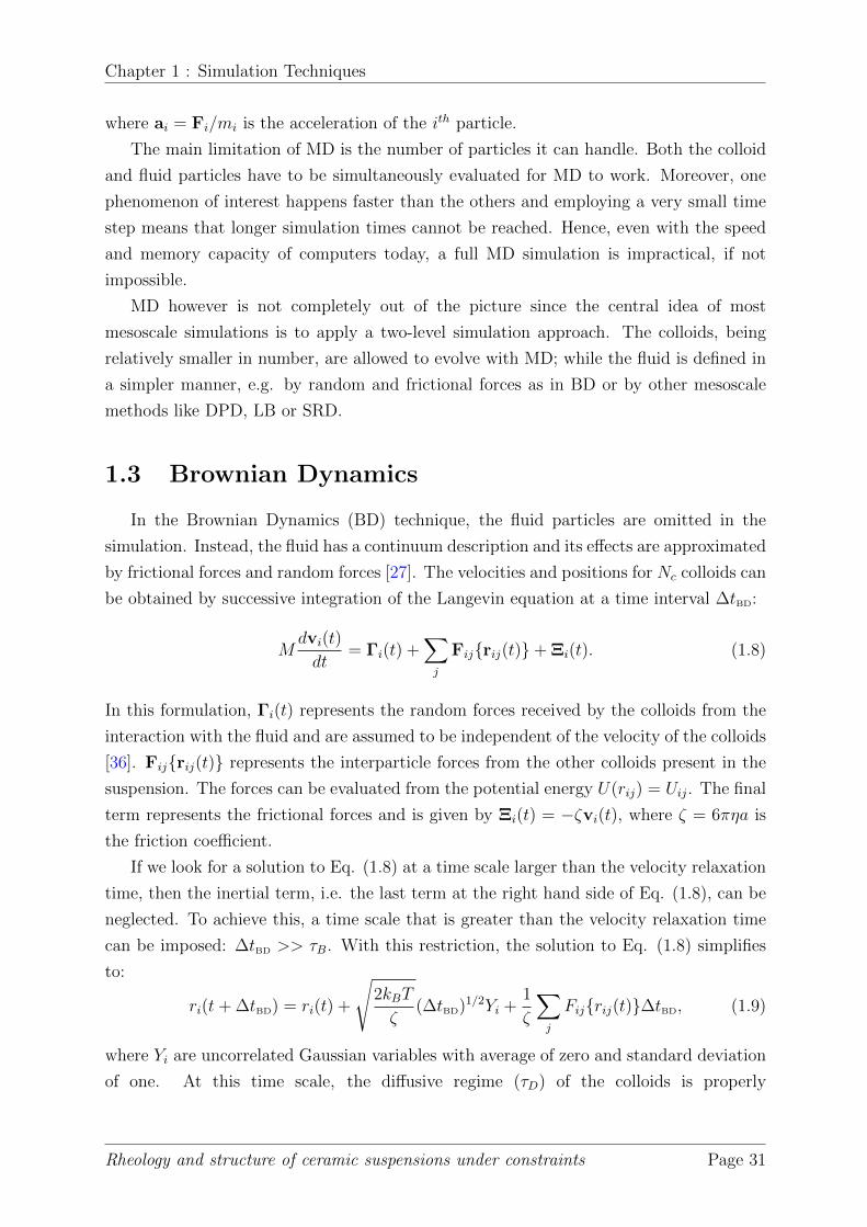
where ai = Fi/mi is the acceleration of the ith particle.
The main limitation of MD is the number of particles it can handle. Both the colloid
and fluid particles have to be simultaneously evaluated for MD to work. Moreover, one
phenomenon of interest happens faster than the others and employing a very small time
step means that longer simulation times cannot be reached. Hence, even with the speed
and memory capacity of computers today, a full MD simulation is impractical, if not
impossible.
MD however is not completely out of the picture since the central idea of most
mesoscale simulations is to apply a two-level simulation approach. The colloids, being
relatively smaller in number, are allowed to evolve with MD; while the fluid is defined in
a simpler manner, e.g. by random and frictional forces as in BD or by other mesoscale
methods like DPD, LB or SRD.
1.3 Brownian Dynamics
In the Brownian Dynamics (BD) technique, the fluid particles are omitted in the
simulation. Instead, the fluid has a continuum description and its effects are approximated
by frictional forces and random forces [27]. The velocities and positions for Nc colloids can
be obtained by successive integration of the Langevin equation at a time interval ∆tBD:
Mdvi(t)
dt= Γi(t) +
∑j
Fij{rij(t)}+ Ξi(t). (1.8)
In this formulation, Γi(t) represents the random forces received by the colloids from the
interaction with the fluid and are assumed to be independent of the velocity of the colloids
[36]. Fij{rij(t)} represents the interparticle forces from the other colloids present in the
suspension. The forces can be evaluated from the potential energy U(rij) = Uij. The final
term represents the frictional forces and is given by Ξi(t) = −ζvi(t), where ζ = 6πηa is
the friction coefficient.
If we look for a solution to Eq. (1.8) at a time scale larger than the velocity relaxation
time, then the inertial term, i.e. the last term at the right hand side of Eq. (1.8), can be
neglected. To achieve this, a time scale that is greater than the velocity relaxation time
can be imposed: ∆tBD >> τB. With this restriction, the solution to Eq. (1.8) simplifies
to:
ri(t+ ∆tBD) = ri(t) +
√2kBT
ζ(∆tBD)1/2Yi +
1
ζ
∑j
Fij{rij(t)}∆tBD, (1.9)
where Yi are uncorrelated Gaussian variables with average of zero and standard deviation
of one. At this time scale, the diffusive regime (τD) of the colloids is properly
Rheology and structure of ceramic suspensions under constraints Page 31

Chapter 1 : Simulation Techniques
reproduced. Moreover, since the velocity correlations decay more rapidly than the time
scale considered, only the positions of the colloids are followed [36].
Among the major consequences of removing the fluid in BD is that HIs are ignored.
On one hand, the elimination of HIs greatly simplifies the computation. This is also the
main reason why the standard BD presented above is extensively utilized and have been
very successful in problems where hydrodynamic effects are negligible [37, 38, 39]. On the
other hand, HIs are omnipresent in nature so that there is also wide range of problems
that require models that correctly account for hydrodynamic effects.
Therefore, it comes as no surprise that BD has been extended to incorporate HIs
[40, 41, 36]. In general this is achieved by making the diffusion coefficient dependent on
the position of the colloids. The incorporation of HIs is usually carried out by employing
diffusion tensors, which represent both the diffusive and frictional effects occuring in
the system. One of the widely used formulation is the Yamakawa-Rotne-Prager (YRP)
diffusion tensor:
Dij = δijkBT
6πηaI +
kBT
8πηrij
(I +
rijrTij
r2ij
)− kBT
8πηr3ij
(2a2)
(rijr
Tij
r2ij
− 1
3I
), (1.10)
when rij > 2a; and
Dij =kBT
8πηa2
[(4a
3− 3rij
8
)I +
rij8
rijrTij
r2ij
], (1.11)
when rij ≤ 2a. The term I is the identity tensor while δij is the Kronecker delta. While
BD-YRP is an improvement from standard BD, this approach is still computationally
intensive and imposes serious limitations on the size of the system that can be studied.
First, one of the most important approximations used to derive this tensor is to consider
that HIs are pairwise additive. This means that the total potential of the system must be
represented as the sum of all two-body interactions, which can be memory consuming. In
addition to this, it does not model short range HIs but only long range HIs. Therefore, this
tensor is generally appropriate for systems with relatively low colloid volume fractions.
Second, from the point of view of computation efficiency, the computational cost increases
drastically with increasing number of Brownian particles Nc since BD-YRP requires tensor
evaluation that scales as O(N2c ) and diagonalization that scales as O(N3
c ).
Rheology and structure of ceramic suspensions under constraints Page 32

Chapter 1 : Simulation Techniques
1.4 Other Mesoscale Methods
1.4.1 Dissipative Particle Dynamics
Dissipative Particle Dynamics (DPD) is developed by Hoogerbrugge and Koelman
in 1992 [5, 4] to address the computational limitations of MD and BD. Moreover, they
showed that DPD mimics the behavior of a Navier-Stokes flow [5]. The DPD particles
can be viewed as static “clumps” of fluid molecules interacting with very soft interparticle
potentials [24, 30]. Since it is an extension of standard MD, the dynamical variables are
evolved similar to Eq. (1.4) where the forces are defined by particle pairs. In general, the
total force is given by[24, 42]:
Fij = Fcij + Fd
ij + Ffij. (1.12)
The term Fcij represents the interparticle forces and Fd
ij represents the velocity-dependent
frictional forces given by
Fdij = −
∑j
ζ(rij) [(vi − vj) · rij] rij (1.13)
where ζ(rij) is the relative friction coefficient for particle pairs and rij is the unit vector
in the direction of rij. The stochastic forces also act along the line of centers:
Ffij =
∑j
ς(rij)ηij rij, (1.14)
where ηij is the noise term and ς(rij) determines the strength of the stochastic force
applied to the particle pair [24]. The advantages of DPD over standard MD and BD are:
(a) it allows a longer time step because of the larger size of DPD particles and the softer
interactions between them; and (b) the DPD particles also interact by velocity dependent
frictional forces which automatically accounts for HIs [24]. There are also several proposed
refinements to the original formulation, which include a mechanism where the solvent can
transfer shear forces to the solute [43, 42]. Similar to BD-YRP however, DPD is still
computationally demanding due to the pairwise forces that require evaluation every time
step.
1.4.2 Lattice-Boltzmann
The Lattice Boltzmann (LB) method is another prominently featured simulation
technique for soft matter systems. LB originated from lattice gas automata, a discrete
particle kinetics utilizing discrete lattices and discrete times. LB has a huge and rich
Rheology and structure of ceramic suspensions under constraints Page 33

Chapter 1 : Simulation Techniques
background starting from the Broadwell model in 1964 [44], which can be viewed as a
one-dimensional lattice Boltzmann equation [45]. In LB, the fluid density at a lattice site
r with velocity ci just prior to the collision is represented by ni(r, t). The discrete time
interval is given by ∆tLB. The system is evolved by using a linearized and preaveraged
Boltzmann equation that is discretized and solved on a lattice:
ni(r + ∆tLBci, t+ ∆tLB) = ni(ri, t)−∆tLB
τLB
[ni(ri, t)− neqi (r, t)] (1.15)
where neqi (r, t) is the local equilibrium value with a time scale τLB that is related to the fluid
viscosity [46]. From the moments of ni(r, t), relevant quantities such as hydrodynamic
field, mass density, momentum density and momentum flux can be obtained. Through the
appropriate constraining of the equilibrium distribution function and using a Chapman-
Enskog expansion, the Navier-Stokes equation is obtained from the linearized Boltzmann
equation.
This described implementation of LB is computationally efficient. While the thermal
fluctuations are not included in its original formulation [47] and the incorporation of
thermal fluctuations was relatively recent and is coined as the Fluctuating Lattice
Boltzmann (FLB) [46] approach, this new development in LB made it a versatile
simulation tool that can be used when thermal fluctuations need to be isolated or added.
1.5 Stochastic Rotation Dynamics
Stochastic Rotation Dynamics (SRD), also known as Multiparticle Collision Dynamics
(MPCD) is first developed by Malevanets and Kapral in 1999 [25, 48, 49]. SRD is a
particle-based approach, where the fluid is represented by Nf point particles. The number
of fluid particles is significantly smaller compared to the number of particles that MD
requires. Moreover, it has a larger length scale than real fluid molecules hence allowing
simulation of longer time scales. SRD can be interpreted as a Navier-Stokes solver that
includes thermal noise [30], where the SRD fluid serves as a convenient way to coarse-grain
the properties of the real fluid. The algorithm is a two-step process: the streaming step
and the collision step that are implemented at regular time intervals ∆tSRD. During each
streaming step, the positions are updated according to the equation:
ri(t+ ∆tSRD) = ri(t) + vi(t)∆tSRD, (1.16)
where ri and vi are the ith particle’s position and velocity respectively.
Unlike the previous mesoscale simulations, the SRD fluid particles are sorted in even
more manageable groups before the collision rule is implemented. This approach of
Rheology and structure of ceramic suspensions under constraints Page 34

Chapter 1 : Simulation Techniques
coarse-graining the fluid significantly simplifies the process. The particles are placed
into “collision cells” of side length a0, where random rotation of velocities takes place.
The choice of a0 is based on colloid size and is set to a/2 in this work. The volume of the
simulation box can be defined such that V = Lx×Ly×Lz = (lx× ly× lz)×a30, where lx, ly
and lz are integers and a30 is the cell volume. Each cell contains an average of γ = 5 fluid
particles. This is the typical value applied in most simulation studies [1, 2, 50] mainly
because it balances computational efficiency and resolution. Particle exchanges between
cells are allowed but the number of fluid particles in the simulation box is conserved and
kept at Nf . The collision per cell is performed by rotating the velocities of the particles
relative to the center of mass velocity vcm according to the equation:
vi(t+ ∆tSRD) = vcm + R(α) [vi(t)− vcm] , (1.17)
where R is a rotation matrix [51]. In three dimensions, the rotation is fixed at an angle α
about a randomly chosen axis. The value of α can range from 0◦ to 180◦. The rotations
by −α need not be considered since this is equivalent to a rotation by α about an axis
with the opposite direction. However, the simplest rotation algorithm is when α is set to
90◦.
The dimensionless mean free path λ is the average fraction of a cell travelled by a fluid
particle during a streaming step. This is given by
λ =∆tSRD
a0
√kBT
mf
, (1.18)
where mf is the mass of the fluid,
mf =a3
0ρfγ
, (1.19)
and ρf is the mass density. If between each collisions, the particles travel a distance
that is smaller that the cell size i.e. λ/a0 << 1, then even after several time steps, the
same particles remain in a given cell and their motion become correlated. This leads to
a breakdown in molecular chaos assumption and Galilean invariance is destroyed. One
way to go around this problem is to choose λ/a0 > 0.5. However this choice of λ would
model a fluid that is “gas-like” rather than “liquid-like” [30]. For a gas, the momentum
transport is dominated by mass diffusion through the streaming of particles; while for
a liquid, momentum transport is governed by interparticle collisions. Hence simulating
a liquid-like behavior would require λ/a0 << 0.5. Following previous studies by Refs.
[1, 2, 30], λ is set to a value of 0.1, which should suffice for the representation of the
hydrodynamics of a liquid.
To restore Galilean invariance assumptions, a grid-shift procedure is employed [1].
Rheology and structure of ceramic suspensions under constraints Page 35

Chapter 1 : Simulation Techniques
Figure 1.1: Schematic diagram of a sample 2-D SRD system with cell size a0, γ = 5 andsimulation box length of L = 4× a0.
This is done by constructing a new cell-grid that is randomly translated at a certain
distance before each collision step. Collisions are performed in the shifted cells thus
allowing exchange of particles. Particles are then reverted back to the original cells and
the SRD process is continued.
The described process conserves linear momentum and mass and is sufficient to ensure
that in the macrsocopic limit, the SRD process recovers the continuity and Navier-Stokes
equations. A schematic diagram of a sample SRD system is shown in Fig. 1.1. By
carefully choosing the values of the SRD parameters (α, a0γ, λ,mf and T ), one can adjust
the properties of the fluid to fit the system being modeled.
1.5.1 Sheared SRD fluid
In this section, the method of implementing shear on particles is discussed. As a
starting point, the shearing of a pure SRD fluid, i.e. without embedded colloids, is
illustrated. In fact, the original formulation of SRD by Malevanets and Kapral [25, 48]
used an equilibrium system so that the introduction of shear by Kikuchi et al. [2] served
as a development of the previous model. This is because shear provides a new numerical
approach for studying the flow behavior of a fluid that can be extended over different
shear magnitudes [2]. A more useful application of shear modeling is geared towards the
understanding of the effects of shearing on the behavior of the embedded particles in the
fluid. From here, one can extend the range of applications of SRD-MD in the study of
rheology of colloidal suspensions. Example cases include shear thinning [31, 52] and other
flow-induced properties [53, 28]. Moreover there are different possibilities of extending
the study of sheared suspensions since the presence of an external force such as shear is
already very common in nature [54].
One of the common approaches used to introduce shear is to confine the fluid particles
in a channel by placing a wall at the top and bottom surfaces of the simulation box and
exposing the SRD-fluid to a constant external force that yields a parabolic flow profile
Rheology and structure of ceramic suspensions under constraints Page 36

Chapter 1 : Simulation Techniques
[53, 55, 56]. In Ref. [53] for example, the walls are considered as consisting of an immobile
monolayer of interaction sites with homogeneous density. The walls are placed at rx = 0
and rx = Lx and are defined by an effective interaction potential given by:
Vwf =
23πεwall
[215
(σwall
rx
)9
−(σwall
rx
)3
+√
103
]rx ≤ (2/5)
16σwall
0 rx > (2/5)16σwall,
(1.20)
where σwall is the interaction parameter between the fluid particles and the wall particles,23πεwall is the effective potential well depth and rx is the distance of the fluid particle from
the wall. Eq. (1.20) is repulsive and only varies perpendicular to the plane defining the
wall. The external force applied is given by:
vz(rx) =g
2ν(Lx − rx)rx, (1.21)
where g is the acceleration constant of the flow, ν = η/ρ is the kinematic viscosity of the
fluid. Hence the shear rate is given by:
γ(rx) =g
2ν(Lx − 2rx). (1.22)
However, this kind of wall representation can lead to wall effects [57] like solid-
fluid boundary conditions and the introduction of pseudo-particles [50]. As an alternate
approach, shear can be introduced by simply modifying the periodic boundary conditions.
This method was proposed by Lees and Edwards [58] for molecular fluids in 1972 and can
easily be adapted for SRD fluids. Unlike the representation of actual walls, Lees-Edwards
boundary conditions (LEBC) do not have these kinds of numerical instabilities since the
simulation of shear is done by merely shifting the simulation boxes. The LEBC work by
updating the positions and velocities of the particles with the usual periodic boundary
conditions for y and z directions. However, when a particle crosses the upper or lower
boundaries of the simulation box i.e. at rx = 0 and rx = Lx, its position and velocity are
updated with a different rule to sustain the shear. Particles crossing the upper boundary
will have an additional velocity of +γLx and a position shift of +γLxt, where t is the total
elapsed time. In contrast, particles crossing the lower boundary will have an additional
velocity of −γLx and a position shift of −γLxt. A planar Couette flow profile is set-up
with a shear rate of
γ =∆vy∆rx
(1.23)
Rheology and structure of ceramic suspensions under constraints Page 37

Chapter 1 : Simulation Techniques
Figure 1.2: Schematic diagram on how LEBC is implemented. Please refer to the textfor more details.
where ∆vy is the shear velocity given by
∆vy =∆ry∆t
(1.24)
Fig. 1.2 shows how LEBC is implemented step by step. At time t = 0, the simulation
boxes are aligned obeying the usual periodic boundary conditions. When there is no
shear, the simulation boxes are stationary and the evolution of the particle position is
only dictated by the inter-particle dynamics. This is illustrated in Fig. 1.2a, where the
change of position only goes from the black circle to the open circle. However when
the shear is applied, aside from the displacement defined by the inter-particle dynamics,
there is also the displacement due to shear. In the example shown in Fig. 1.2b, the
top simulation boxes will move to the right at a distance of ∆ry after the first time step
t = ∆t. Hence the particle will first move from the black circle to the open circle due
to the interparticle dynamics; then the particle will move from the open circle to the
gray circle by a distance ∆ry due to the shear. The gray circle represents the final ry
coordinate of the particle. The shifted distance of the particle depends on the total time
elapsed t = n∆t, where n is an integer, and the shear velocity ∆vy (see Figs. 1.2c and
1.2d). The same algorithm is applied on the simulation boxes at the bottom, only that
the boxes move in the opposite direction. For reference, a sample fortran code is shown
below.
The value DELVY corresponds to the shear velocity ∆vy while totaltime and
Rheology and structure of ceramic suspensions under constraints Page 38

Chapter 1 : Simulation Techniques
ashift = DELVY * totaltime
dely = ashift - anint(INVLENGY * ashift) * LENGY
corx = anint(INVLENGX * x - 0.5)
y = y - corx * dely
vy = vy - corx * DELVY
y = y - LENGY * anint(INVLENGY * y - 0.5)
x = x - LENGX * anint(INVLENGX * x - 0.5)
z = z - LENGZ * anint(INVLENGZ * z - 0.5)
dely store the total time and distance traveled by the simulation boxes respectively.
Moreover since LEBC can maintain a linear velocity profile, the shear vicosity can be
measured once the system reached a steady-state condition.
Further probing of rheological behavior can be obtained by changing the motion of
the walls. Oscillatory walls for example can be used to measure the zero-shear viscosity
limit or in the case employed in this thesis, to determine the self-assembly of the colloids
within the aggregate. To simulate an oscillating motion for the walls, one simply needs
to replace DELVY by a time-dependent velocity dvy given by:
dvy = DELVY * cos ( 2 * pi * totaltime * FREQ )
In this formulation, DELVY now describes the amplitude of oscillation while
FREQ dictates the frequency of oscillation of the system. With this algorithm of
introducing shear, the modulation of shear forces can easily be achieved.
1.5.2 Thermostats
Following the introduction of shear in the system is the use of a thermostat. The SRD
fluid used in this work samples a microcanonical ensemble i.e. the energy of the system
must be constant in time. A thermostat is a modification of the original simulation
algorithm with the motivation of generating a microcanonical ensemble. Thermostats are
usually employed to match the experimental conditions, to study temperature-dependent
processes, to avoid energy drifts caused by the accumulation of numerical instabilities and
for the purposes of this work, to dissipate heat in non-equilibrium conditions and ensure
a steady-state condition [59]. Over the years, most of the thermostats developed are for
MD [60, 61, 62]. However, since SRD is also a particle-based technique, some of these
thermostats can be adapted to suit the SRD fluid [52].
To begin the understanding of the thermostat algorithm, there are several
temperatures to be defined. First is the reference temperature T0, to which the
temperature of the sytem is driven. This value is set to T0 = 293 K in this work so that
the systems studied are at room temperature. Next is the instantaneous temperature
Rheology and structure of ceramic suspensions under constraints Page 39

Chapter 1 : Simulation Techniques
given by
T =2
3kBNK, (1.25)
where K is the kinetic energy:
K =1
2
N∑i
mi(v2i − v2
cm). (1.26)
According to Hunenberger [59], temperature fluctuations characterize the rate of energy
transfer from the heat bath to the system. The spread of this fluctuations is given by
σT =√〈T 2〉NV T − 〈T 〉2NV T = 2NT. (1.27)
Finally, T is the average temperature of the system that is checked every time step.
1.5.2.1 Simple Scaling Thermostat
One of the commonly used thermostats is the simple scaling thermostat. In this
method, the scaling factor S is chosen such that
S =
√3NfkBT0
2∑Nf
i mi(v2i − v2
cm). (1.28)
This kind of thermostat can be used for fluids in equilibrium and was employed in Ref. [63]
for the calculation of diffusion coefficient. However, it tends to show instabilities for fluids
under external shear. In most equilibrium systems, the simple scaling of temperature
should suffice. However, one needs to note that the energy fluctuations are incompatible
with an isothermal ensemble so that the distribution of velocities in a collision cell is
no longer Maxwellian [52]. The smearing of velocity distribution profiles can have a
huge effect in the calculation of viscosity, hence a good thermostat is an integral part of
modeling suspensions under shear.
1.5.2.2 Monte-Carlo Thermostat
Thermostats permitting fluctuations are more likely to represent the correct dynamics
of the systems than the simple scaling thermostat. To answer the requirements of the
system at hand, an alternative cell-level thermostat is used. The Monte-Carlo thermostat
is a computationally efficient thermostat for SRD that accounts for the coarse-graining
by collision cells. The original formulation was by Heyes [64] for molecular fluids and was
adapted in Ref. [31, 65] for SRD-MD. This method also conserves the linear momentum
and temperature of the system without smearing out the velocity profile, or changing the
Rheology and structure of ceramic suspensions under constraints Page 40

Chapter 1 : Simulation Techniques
Figure 1.3: The effect of varying the thermostat strength c on the system temperature.
viscosity of the fluid [29]. Ref. [29] outlined the algorithm as follows.
First, the strength c of the thermostat is dictated. A higher c corresponds to a stronger
thermostat. Second, a number is randomly chosen in the range ψ ∈ [1, 1 + c] and the
scaling factor is given a value of either S = ψ or S = ψ−1, each having a probability of
1/2. Third, another random number is chosen in the range ξ ∈ [0, 1]. If ξ is less than the
acceptance probability that is given by pA = min(1, A), where
A = S3(γ−1) exp
[− mf
2kBT0
∑i=1
(vi − vcm)2{S2 − 1
}], (1.29)
then the velocities are rescaled by scaling the rotation matrix SR in Eq. (1.17). Otherwise,
the rotation matrix is kept at R. This thermostat produces a Maxwellian velocity
distribution and does not change the viscosity of the fluid. Moreover, the collision rule
can be varied as long as the correct macroscopic conservation laws, such as mass, number
density and momentum are conserved [66]. The use of the thermostat means that the
energy is not conserved in the original implementation of SRD, however it is retained in
the statistical sense. To demonstrate how the the thermostat works, Fig. 1.3 shows how
thermalization occurs in a system for various thermostat strengths. A high magnitude of
c can drive the temperature to a lower value faster than a c with a relatively smaller
magnitude. The value of c can be adjusted until the correct system temperature is
achieved. Therefore, several time steps are required before proceeding with the actual
measurements to ensure that the temperature is at the desired value.
1.5.3 Coupling SRD with MD
After treating SRD and MD separately (Secs. 1.2 and 1.5), one can proceed with the
SRD-MD model wherein the fluid-fluid interactions are treated using SRD as described
Rheology and structure of ceramic suspensions under constraints Page 41

Chapter 1 : Simulation Techniques
above and the colloid-colloid interactions are treated by MD. For the MD part, the choice
of interaction potential in Eq. 1.5 depends on the system in question. In the simplest
case, one can use the inverse-power (IP) potential of the form:
Ucc =
εcc(σccr
)12(r < rcc)
0 (r > rcc),
(1.30)
where εcc = 2.5kBT and rcc = 2.5σcc. The variable σcc is the colloid interaction parameter
set to σcc = d = 2a.
On the other hand, the colloid-fluid dynamics can be described either by SRD as
in Refs. [31, 65, 67], where the colloids are treated as point particles from the point
of view of the fluid particles; or by MD, where the colloids have a non-vanishing size.
A schematic diagram is shown in Fig. 1.4. Ref. [68] explored the differences between
the two coupling schemes and found that the effects of HI’s on diffusion coefficient and
conductivity are more pronounced when MD is used. Since shear viscosity is more sensitive
to hydrodynamic effects than diffusion and conductivity, an MD coupling scheme is more
suitable for its calculation.
The MD coupling proceeds by summing the three different types of interactions present
in the colloidal suspension: interactions between colloids that occur at MD time-scale
(∆tMD), interactions between fluid particles that occur at SRD time-scale (∆tSRD), and
interactions between colloids and fluid particles that occur at MD time-scale. The fluid-
fluid interaction potential Vff is set to zero. Hence the interactions among fluid particles
are solely described by SRD. For the dynamics between colloids and fluids we use an IP
potential which is similar in form as in Eq. 1.30 but with the parameters corresponding
to colloid-fluid interactions:
Ucf =
{εcf(σcf
r
)12(r < rcf )
0 (r > rcf ),(1.31)
where εcf = 2.5kBT and rcf = 2.5σcf . Unlike σcc, the choice of σcf is not as straight-
forward since the colloids are viewed as solid interfaces moving with respect to the fluid.
To determine the appropriate value for σcf , the following considerations must be made.
The colloid-fluid boundary can be categorized to stick, slip or mixed boundary
conditions [69]. The stick boundary condition is also known as no-slip boundary condition.
This is the case where the tangential component of the fluid velocity vanishes at the
interface. The corresponding frictional coefficient is ζ = 6πηa. Both the linear and
angular momentum are conserved in this set-up. On the other hand, in the slip boundary
conditions, the tangential component of the fluid is unaffected by the presence of the
Rheology and structure of ceramic suspensions under constraints Page 42

Chapter 1 : Simulation Techniques
Figure 1.4: The two kinds of coupling for SRD-MD. On the left is by SRD where thecolloids are treated as point particles from the point of view of the fluid and on the rightis by MD where the colloids are treated as spheres with volume 4πσ3
cf/3
interface. This set-up conserves the linear momentum but does not transfer angular
momentum. The corresponding frictional coefficient is ζ = 4πηa. Despite the absence
of angular momentum conservation however, the shear viscosity of the pure fluids can
still be accurately obtained [69]. Note however that physical systems resembles partial
slip boundary conditions that lies in between the stick and slip definitions. In the mixed
boundary conditions, the relative tangential velocity of the fluid is diminished near the
surface but remains zero [69].
The MD-coupling scheme that is employed in this work leads to an effective slip
boundary conditions, hence the friction coeffcient ζ = 4πηa is used. The consequences of
this manner of coupling are as follows. First, it is important to choose σcf to be slightly
less than the colloid radius a to avoid unphysical depletion attraction between colloids.
Depletion forces are due to spurious interactions that arise from the coarse-grained nature
of the fluid when colloids approach each other at short distances [30, 70]. In this work,
σcf = 0.8a is implemented. Subsequently, the fluid particles can slightly penetrate the
surface of the colloids. Even when the colloids are in contact, the fluid particles can slide
between the colloids thus adding lubrication to colloid-colloid interactions. Second, the
free volume accessible to the fluid particles is now dictated by σcf rather than a. This is
defined by
Vf = (32a0)3 −Nc4
3πσ3
cf (1.32)
where Nc is the number of embedded colloids. In addition, we know from Ref. [63] that the
Schmidt number (Sc) of the fluid increases with increasing number of colloids. To keep
Sc constant with increasing volume fraction, the number of fluid particles is decreased
according to Vf i.e.
Nf = 323γ −Nc4
3π
(σcfa0
)3
γ. (1.33)
Finally, if the SRD-coupling is used, the colloids directly undergo the thermostat
algorithm with the fluid particles during the rotation steps. For the MD-coupling on the
Rheology and structure of ceramic suspensions under constraints Page 43

Chapter 1 : Simulation Techniques
other hand, there is no actual thermostat algorithm that is applied to the colloids but
the interactions between the colloids and the fluid during the MD steps allow both colloid
and fluid particles to be thermally coupled.
1.6 Mapping between physical and SRD-MD time
scales
We have seen that the system consisting of colloids embedded in the fluid has several
parameters that can be adjusted to provide the desired properties for the model. This
section focuses on determing the values of these parameters in order to map the simulation
scales to physical scales.
As mentioned in Sec. 1.1, the mesoscopic nature of colloidal suspensions results to
a wide range of time scales. SRD-MD compresses this hierarchy of times scales so that
only one time scale can be accurately reproduced. There are two significant time scales
to which the mapping is usually done: the diffusion time scale τD and the kinematic
time scale τν . SRD-MD gives the liberty of selecting the fastest time scale to optimize
the simulation. This contraction has the consequence that some physical quantities take
values that are far from the actual experimental values. For example, a system mapped
to the diffusion time scale will give the wrong magnitude of shear viscosity but the correct
magnitude of the diffusion coefficient. However, a system mapped in kinematic time scale
will give a wrong magnitude for diffusion coefficient but a correct magnitude for shear
viscosity. As mentioned in Ref. [30], the quantitative value is not important as long as
the correct regime of the hydrodynamic numbers is obtained and the different time scales
are well separated. The diffusion time scale is used in this study because it significantly
reduces the computation time by allowing the use of bigger time steps. Hence longer times
scales can be reached at faster rates. Nevertheless, it is important to account for these
changes in magnitude and determine the appropriate time scale for a specific system.
To map to the diffusion time scale, one first needs to calculate the physical diffusivity
of a colloid in water. This is given by
D0 =kBT
(6πηH2Oa). (1.34)
Notice that in Eq. 1.34, the friction coefficient is the one that correponds to stick boundary
conditions. Since slip boundary conditions are applied in the simulated systems, the
friction coefficient used in Eq. (1.34) is equated to the simulated friction coefficient.
To solve for the corresponding diffusion coefficient in the SRD-MD simulations (DSRD),
it is important to note that the friction coefficient of the SRD fluid in the simulations
Rheology and structure of ceramic suspensions under constraints Page 44

Chapter 1 : Simulation Techniques
has two components [30]. The first one comes from the Brownian collisions and can be
calculated by a simplified Enskog-Boltzmann-type kinetic theory that is adapted for slip
boundary conditions. This is given by
ζE =8
3
(2πkBTMcmf
Mc +mf
)1/2
nfσ2cf , (1.35)
where nf = γ/a30. Since a0λ/(∆tSRD) =
√kBT/mf , Eq. (1.35) can be written as
ζE =8
3
(2π
Mc
Mc +mf
)1/2
γ
(σcfa0
)2mfλ
∆tSRD
= ξEmfλ
∆tSRD
, (1.36)
where
ξE =8
3
(2π
Mc
Mc +mf
)1/2
γ
(σcfa0
)2
. (1.37)
The other contribution comes from Stokes friction that derives from integrating the Stokes
solution to the hydrodynamic field over the surface of the particle at r = σcf [30]. The
Stokes friction can be written as
ζS =4πησcff(σcf/L)
, (1.38)
where f is the correction factor that accounts for finite size effects. The factor f scales as
f(σcf/L) ≈ 1− 2.837σcfL. (1.39)
Another way to express the Stokes friction coefficient is to use the analytical definition of
viscosity given by η = νγmf/a30 and to neglect the correction factor. This gives
ζS = 4π
(νkin + νcol
ν0
)γσcfa0
mfλ
∆tSRD
= ξSmfλ
∆tSRD
, (1.40)
where
ξS = 4π
(νkin + νcol
ν0
)γσcfa0
. (1.41)
From Eqs. 1.37 and 1.41, the friction coefficient of the SRD fluid can be written as
ζSRD =
(1
ξS+
1
ξE
)−1mfλ
∆tSRD
. (1.42)
Thus, the diffusion coefficient for a single colloid can now be written as
DSRD =kBT
ζ=
1
ξ
a20
t0, (1.43)
Rheology and structure of ceramic suspensions under constraints Page 45

Chapter 1 : Simulation Techniques
where ξ = (1/ξS + 1/ξE)−1. From the expression of diffusion, one has
τD =a2
DSRD
≈σ2cf
DSRD
= ξ
(σcfa0
)2∆tSRD
λ. (1.44)
Finally, from τD, the corresponding ∆tSRD time step can be obtained using the equation:
∆tSRD =λτDξ
(a0
σcf
)2
. (1.45)
A similar technique can be applied to map to other time scales. An example mapping to
kinematic time scale is discussed in Ref. [30].
Since the length and times scales are rescaled in SRD-MD, other variables such as the
temperature and energy are also rescaled. Similar to the transport coefficients, the actual
temperature is mapped from experimental scale to SRD scale and vice versa. A system
temperature of T0 = 293 K is equivalent to an SRD temperature of
TSRD =a2
0mf
kBt20. (1.46)
Consequently, the unit of energy is given by kBTSRD.
1.7 Summary
A brief summary of the different methods discussed in this chapter is given in Table 1.2.
While each of these techniques have their own merits, the efficiency of a simulation method
greatly depends on the problem in question. In most of the colloidal systems studied
numerically, the two most relevant suspension properties that need proper modeling are
Brownian motion and HIs. In this regard, it is important to note that BD is the fastest
numerical tool available for systems where HIs can be ignored. In the same manner, SRD-
MD remains as the simplest simulation technique for systems where HIs are significant.
Moreover, the two methods can be simultaneously used to isolate the effects of HIs.
The next chapter deals with the calculation of the viscosity of sheared colloidal
suspensions, which will serve as a validation of the effectiveness of the SRD-MD model
described in this chapter.
Rheology and structure of ceramic suspensions under constraints Page 46

Chapter 2: Shear Viscosity
Table 1.2: Brief summary of mesoscopic simulation techniques
Model Brownian motion HIs Typestandard BD 3 7 continuum-basedBD-YRP 3 3 continuum-basedDPD 3 3 particle-basedstandard LB 7 3 lattice-basedFLB 3 3 lattice-basedSRD 3 3 particle-based
Rheology and structure of ceramic suspensions under constraints Page 47

Chapter 2: Shear Viscosity
Chapter 2 :
Shear Viscosity
Rheology and structure of ceramic suspensions under constraints Page 48

Chapter 2: Shear Viscosity
Calculating the shear viscosity of a suspension is a model problem for studying the
rheological behaviour of mesoscopic systems [71, 72]. Specifically, there have been plenty
of studies of suspension viscosity as a function of the particle concentration. It is a key
parameter for investigating several experimental phenomena such as phase transitions
and yield stress. Moreover, theoretical models for the behaviour of shear viscosity as a
function of concentration are relatively well-known [9, 10, 73, 74] so that it can be used
as a benchmark to validate an evolving numerical model. Once validated, one can easily
shift to analyze the dependence of shear viscosity on other relevant variables such as shear
rate, particle structure, Peclet number (Pe) and Reynolds number (Re).
The system used in the calculation of shear viscosity is based on hard-sphere colloids
mainly because their properties are theoretically and numerically well-known as compared
to systems with more complex interactions. While it has been shown in Ref. [31]
that SRD-MD can be used to calculate viscosity using a DLVO description for colloid-
colloid interactions, it is important to justify that the computation of shear viscosity
using SRD-MD agrees with existing theoretical predictions and can reproduce results
that are comparable with other simulation techniques. Every good numerical method
should correctly reproduce the behaviour of the shear viscosity as a function of volume
fraction. To do this, employing a hard-sphere description of the colloids is sufficient and
more practical.
The objective of this chapter is to provide a quantitative test on the ability of SRD-
MD to model HI’s on colloidal suspensions by calculating its shear viscosity. Specifically,
this chapter will demonstrate that SRD-MD can be used for both dilute and concentrated
cases. The first step in doing this is to understand that there are two ways to calculate
shear viscosity: the equilibrium approach and the non-equilbrium approach. From the
name itself, the equilibrium approach is suited for liquids in equilibrium while the non-
equilibrium approach is for liquids under shear. Both approaches require an expression for
the stress tensor of the liquid, the main ingredient for the calculation of shear viscosity.
The stress tensors and shear viscosities of pure fluids in equilibrium and non-equilibrium
are presented first. The idea is then developed to accommodate the calculation of viscosity
when there are embedded colloids. The calculated results are compared with known
numerical results, theoretical predictions and experimental data.
2.1 System
The colloids to be modeled are silica particles with radius of a = 300 nm, density of
ρc = 2200 kg·m−3 and mass of M = 2.49×10⁻¹⁶ kg. From these given colloidal properties
and from the information provided in Secs. 1.5 and 1.6, the corresponding parameters of
the SRD fluid are derived. The SRD parameters used in this chapter are listed in Table
Rheology and structure of ceramic suspensions under constraints Page 49

Chapter 2: Shear Viscosity
Table 2.1: Parameters used in the calculation of shear viscosity for the pure fluid case
a 300 nm mf 6.75× 10⁻¹⁹ kga0 150 nm ∆tSRD 7.37× 10⁻⁵ sα 90◦ TSRD 2.02× 10⁻³ Kλ 0.1 L 32a0
γ 5 γ 100 s−1
2.1.
The mass and size of alumina colloids are used here only to set the scale of these
quantities. However, since the objective is to compare the calculated results with known
results for hard spheres, the colloids will not interact by the DLVO potential for alumina
in water, but by a potential which resembles a hard-sphere interaction. For a purely
repulsive system, the inverse power potential (IP-12) that appears in Eqs. 1.30 and 1.31
is utilized:
Uij(r) =
{ε(σr
)12for r ≤ 2.5σ;
0 for r > 2.5σ,(2.1)
where ε = εcc = εcf = 2.5kBT , σcc = 2a and σcf = 0.8a.
Note that the diffusion time τD = a2/D0 = 0.12 s is used. The corresponding time step
is ∆tSRD = 7.37×10⁻⁵ s. This is obtained by using the viscosity of water ηH2O = 0.001 Pa·sand the diffusion coefficient of a colloid in water D0 = kBT/(6πηH2Oa) = 7.15× 10⁻¹³ m2
s−1. If instead the kinetic time scale is used, the resulting unit of time is ∆tSRD = 1.12×10⁻⁹ s. Hence the option to map in diffusion time significantly reduces the computation
time by up to 104.
The initial velocities of the particles obey a Maxwell-Boltzmann distribution and are
allowed to evolve using SRD and MD algorithms. When shear is applied however, the
infinite periodic system is subjected to a uniform shear in the xy plane using LEBC. Shear
is applied in the y direction and the gradient is along the x direction. The shear rate is
defined as
γ =∆vy∆x
, (2.2)
where ∆vy is the shear velocity.
For the molecular dynamics part, the value of ∆tMD is smaller than ∆tSRD and generally
depends on the steepness of the potential. It was found that ∆tMD = ∆tSRD/8 is sufficient
to resolve the correct Newtonian dynamics for the IP potential used in this chapter.
Moreover, similar ∆tMD is used in Refs. [63, 75].
Rheology and structure of ceramic suspensions under constraints Page 50
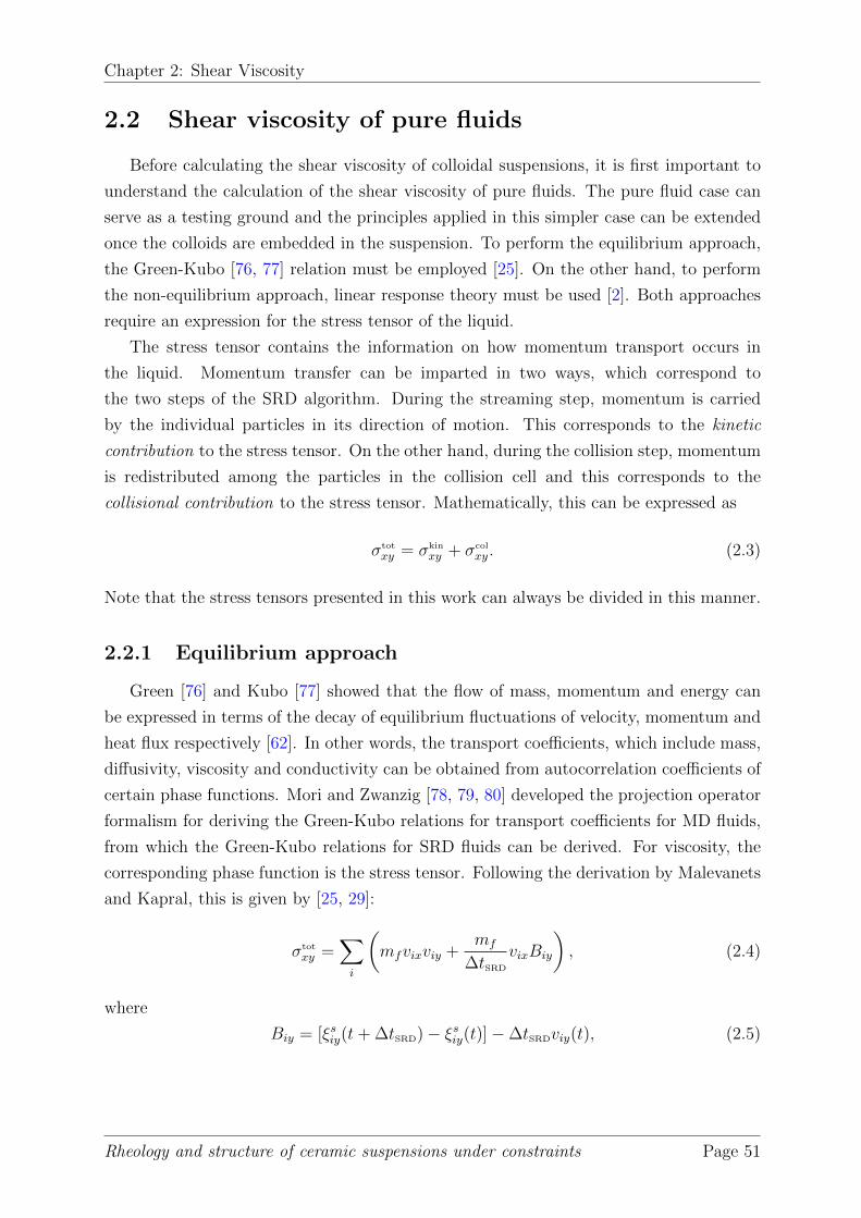
Chapter 2: Shear Viscosity
2.2 Shear viscosity of pure fluids
Before calculating the shear viscosity of colloidal suspensions, it is first important to
understand the calculation of the shear viscosity of pure fluids. The pure fluid case can
serve as a testing ground and the principles applied in this simpler case can be extended
once the colloids are embedded in the suspension. To perform the equilibrium approach,
the Green-Kubo [76, 77] relation must be employed [25]. On the other hand, to perform
the non-equilibrium approach, linear response theory must be used [2]. Both approaches
require an expression for the stress tensor of the liquid.
The stress tensor contains the information on how momentum transport occurs in
the liquid. Momentum transfer can be imparted in two ways, which correspond to
the two steps of the SRD algorithm. During the streaming step, momentum is carried
by the individual particles in its direction of motion. This corresponds to the kinetic
contribution to the stress tensor. On the other hand, during the collision step, momentum
is redistributed among the particles in the collision cell and this corresponds to the
collisional contribution to the stress tensor. Mathematically, this can be expressed as
σtot
xy = σkin
xy + σcol
xy . (2.3)
Note that the stress tensors presented in this work can always be divided in this manner.
2.2.1 Equilibrium approach
Green [76] and Kubo [77] showed that the flow of mass, momentum and energy can
be expressed in terms of the decay of equilibrium fluctuations of velocity, momentum and
heat flux respectively [62]. In other words, the transport coefficients, which include mass,
diffusivity, viscosity and conductivity can be obtained from autocorrelation coefficients of
certain phase functions. Mori and Zwanzig [78, 79, 80] developed the projection operator
formalism for deriving the Green-Kubo relations for transport coefficients for MD fluids,
from which the Green-Kubo relations for SRD fluids can be derived. For viscosity, the
corresponding phase function is the stress tensor. Following the derivation by Malevanets
and Kapral, this is given by [25, 29]:
σtot
xy =∑i
(mfvixviy +
mf
∆tSRD
vixBiy
), (2.4)
where
Biy = [ξsiy(t+ ∆tSRD)− ξsiy(t)]−∆tSRDviy(t), (2.5)
Rheology and structure of ceramic suspensions under constraints Page 51

Chapter 2: Shear Viscosity
and ξsiy is the shifted cell coordinate due to the grid-shift procedure. Eq. (2.5)
represents the difference between the shifted cell coordinate of particle i from ξsiy(t) to
ξsiy(t+ ∆tSRD) during one streaming step and the actual distance traveled by the particle
∆tSRDvjy(t). The Green-Kubo relations for SRD are different from the MD versions
because of the underlying cell structure and multiparticle interactions. For comparison,
the corresponding stress tensor for molecular fluids is given by [27, 29]
σtot
xy =∑i
δ(r− ri)
(mvixviy +
1
2
∑j 6=i
rijxFijy(rij)
). (2.6)
For both Eqs. 2.4 and 2.6, the first terms are the kinetic contributions while the second
terms are the collisional contributions. It can be noticed that the kinetic part is the
same but the collisional part is different. This is because unlike the force definition of
molecular fluid i.e. Fijy(rij) , the force in the SRD fluid is mvix/∆tSRD, which corresponds
to a non-local force at the cellular-level that only acts at discrete time intervals ∆tSRD.
The numerical calculation of shear viscosity can therefore be obtained by integrating
the autocorrelation function of Eq. (2.4). An example formulation is given in Ref. [27]:
η0 = limt→∞
V
kBT
∫ t
0
dt′〈σtot
xy (t′)σtot
xy (0)〉. (2.7)
Malevanets and Kapral also calculated an analytical expression for the shear viscosity
of a pure fluid. This was achieved by using Chapman-Enskog expansion to map the
simulation equations onto the Navier-Stokes equation. By using the following values
α = 90◦, λ = 1 and ∆tSRD = 1 for the rotation angle, dimensionless mean-free path and
time step respectively, the resulting equation presented in Ref. [25] has the form:
η0 =γkBT
6
3(1− e−γ) + 2γ
[e−γ − (1− γ)], (2.8)
where η0 is the shear viscosity of the SRD fluid. This equation shows the dependence of
shear viscosity on the density of fluid particles per cell γ. Note that in general, the shear
viscosity of the SRD fluid depends on the SRD parameters, which will be more apparent
in the succeeding sections.
2.2.2 Non-equilibrium approach
While the use of Green-Kubo relation is more common for pure fluids and is the original
approach used by Malevanets and Kapral [25], the non-equilibrium approach by Kikuchi
et al. [2] is an alternative method that allows the study over a wide parameter range
of shear magnitudes. Moreover, the equilibrium approach is prone to fluctuations and
Rheology and structure of ceramic suspensions under constraints Page 52

Chapter 2: Shear Viscosity
has poor statistics so that long simulation times and averaging over several independent
simulations are required for accurate shear viscosity calculations [27]. It is important to
note these fluctuation effects since they could lead to even longer computation times once
colloids are embedded in the fluid. The stress autocorrelation function can be defined as:
σxy = η0γ. (2.9)
So that obtaining η0 is straight-forward once an expression for σxy is known. The applied
shear γ results to a shear gradient of ∂ux/∂y. Kikuchi et al. have shown that the stress
tensor can be derived and has the form:
σxy =mfγ
a30
(γ∆tSRD
2〈v2y〉 − 〈vxvy〉
), (2.10)
where the averaging is done over the steady-state velocity probability distribution function
of the fluid particles P (vx, vy). It is also important to emphasize that P is not Maxwellian
since in the non-equilibrium steady state, shear induces correlations between vx and vy
[29]. Hence the autocorrelation function does not decay to zero.
Eq. (2.10) can be evaluated by separating the effects of the kinetic and collision part.
For the kinetic part, it can be shown that after the streaming step, the second term
reduces to
〈vxvy〉after = 〈vxvy〉 − γ∆tSRD〈v2y〉. (2.11)
For the collision part, the momentum is redistributed among the particles and the
averaging is done over the rotation matrix. The corresponding term is
〈vxvy〉after = f〈vxvy〉before, (2.12)
where f is given by
f =
{1− γ − 1 + e−γ
γ[1− cos(2α)]
}. (2.13)
Combining Eqs. 2.12 and 2.13 yields:
(〈vxvy〉 − γ∆tSRD〈v2
y〉)f = 〈vxvy〉 (2.14)
〈vxvy〉 = γ∆tSRD〈vy〉2f
1− f. (2.15)
Using Eq. (2.10) and assuming equipartition of energy 〈vy〉2 = kBT/mf , the total stress
tensor can be expressed as:
σtot
xy =γγ∆tSRDkBT
mf
(1
2+
f
1− f
). (2.16)
Rheology and structure of ceramic suspensions under constraints Page 53

Chapter 2: Shear Viscosity
In 2D, the kinetic component of the shear viscosity from Eq. (2.16) reduces to Eq. (2.8)
for α = 90◦ and ∆tSRD = 1. Hence the analytical results of both the equilibrium [25] and
non-equilibrium [2] approach are consistent.
Since these results are for the pure fluid case, the measured viscosity is independent
of the shear rate. However, for very low shear rates, there can be some deviations due
to statistical errors since the applied perturbation is small. On the other end, high shear
rates can lead to finite size effects. This happens when the distance traveled by the walls
in the LEBC approach the size of the system [2].
For “gas-like” systems i.e. λ > a0/2, the collisional contribution of the viscosity is
negligible and the shear viscosity is dominated by the kinetic contribution. Inversely, for
“liquid-like” systems i.e. λ << a0/2, the shear viscosity is dominated by the collisional
contribution and the kinetic part is very small.
2.2.3 Winkler’s formulation
2.2.3.1 Equilibrium case
Winkler and Huang in Ref. [50] have independently derived the stress tensor for SRD-
MD, both for the equilibrium and non-equilibrium cases. This is briefly described in this
section. Starting with Newton’s equation of motion:
mf∂2ri∂t2
= Fi, (2.17)
where ri is the position of the particle in an infinite system without accounting for the
mirror images. If a shear velocity along the y axis and a gradient along the x axis are
used, multiplying Eq. (2.17) by ri and summing over all fluid particles Nf yields,
d
dt
Nf∑i=1
mfviyrix =
Nf∑i=1
mfviyvix +
Nf∑i=1
Fiyrix. (2.18)
When averaged over time, Eq. (2.18) leads to⟨Nf∑i=1
mfviyvix
⟩+
⟨Nf∑i=1
Fiyrix
⟩= 0. (2.19)
Expanding the second term in Eq. (2.19),
〈Fiyrix〉 = limt→∞
1
t
∫ t
0
Fiy(t′)rix(t
′)dt′. (2.20)
Rheology and structure of ceramic suspensions under constraints Page 54

Chapter 2: Shear Viscosity
where t is the total elapsed time. As mentioned in Sec 2.2.1, the collision algorithm
results to a pseudo-force, which is obtained from the change in the momentum during the
collision step at discrete time intervals. This can be rewritten as
Fi(t) =∞∑q=0
mf∆viy(t)δ(t− tq). (2.21)
Using the definition for the time average:
〈...〉T = limN→∞
〈...〉N = limN→∞
1
N
N∑q=1
, (2.22)
Eq. (2.20) can now be written as
〈Fiyrix〉 = limN→∞
1
N
N∑q=1
1
∆tSRD
∫ tq
tq−∆tSRD
mf∆viy(t′)rix(t
′)δ(t′ − tq)dt′
= limN→∞
mf
N∆tSRD
N∑q=1
∆viy(tq)rix(tq), (2.23)
where N is the total number of time steps. When periodic boundary conditions are taken
into account, the positions ri is written as
ri(t) = r′i(t) +Ri(t), (2.24)
where r′i is the mirror image of ri and Ri is the lattice vector at time t. Incorporating
this expansion in Eq. (2.23), one obtains:
〈Fiyrix〉 = limN→∞
mf
N∆tSRD
N∑q=1
[∆viy(tq)r′ix(tq) + ∆viy(tq)Rix(tq)] (2.25)
=mf
∆tSRD
〈∆viy(tq)r′ix(tq) + ∆viy(tq)Rix(tq)〉T . (2.26)
Now that the forces of the system are properly represented, the stress tensor can be
obtained by using the mechanical definition of stress
σxy =FyAx
(2.27)
where Fy is the total force in the direction y across a surface Ax that is normal to the
x direction. Notice that Eq. (2.25) has two parts. The first term is the instantaneous
internal stress tensor and the second term is the instantaneous external stress tensor. The
Rheology and structure of ceramic suspensions under constraints Page 55

Chapter 2: Shear Viscosity
derivation provided in Ref. [50] showed that these two terms can be reduced to:
σintxy = −mf
V
Nf∑i=1
vixviy −mf
V∆tSRD
Nf∑i=1
∆viyr′ix, (2.28)
and
σextxy =mf
V∆tSRD
Nf∑i=1
∆vixRix, (2.29)
respectively. Moreover, the time averages of Eqs. 2.28 and 2.29 are shown to be equal:
σextxy = σintxy in Ref. [50]. In this work, the internal stress tensor is used for the system
since its expression is more complete i.e. it consists of both the kinetic and collisional
parts [50].
2.2.3.2 Non-equilibrium case
The derivation of the stress tensor for systems in equilibrium can be extended to
incorporate LEBC. When shear is imposed, an additional term d(γrix)/dt = γvix is added
on both sides of Eq. (2.18). Hence
d
dt
Nf∑i=1
mf (viy − γrix)rix =
Nf∑i=1
mf (viy − γrix)vix +
Nf∑i=1
Fiyrix − γNf∑i=1
mfvixrix. (2.30)
Similar to the periodic boundary conditions, the time average of the derivative on the left
hand side reduces to zero. Following the same procedures as above, the time average of
the remaining terms can be written as
〈(viy − γrix)vix〉T = 〈vixv′iy〉T +γ∆tSRD
2〈vix〉T . (2.31)
The internal stress tensor is given by
σintxy = −mf
V
Nf∑i=1
v′ixviy −mf
V∆tSRD
Nf∑i=1
∆viyr′ix −
γmf∆tSRD
2V
Nf∑i=1
v2ix (2.32)
where the (′) symbol correponds to quantities that are measured after LEBC are imposed,
vα = vα(t − ∆t) and ∆viy = (viy − viy) are also used. By separating the kinetic and
Rheology and structure of ceramic suspensions under constraints Page 56

Chapter2:ShearViscosity
0
5e-09
1e-08
1.5e-08
2e-08
2.5e-08
3e-08
0 20 40 60 80 100 120 140 160 180
η (Pa • s)
α (degrees)
ηkinηcol
Figure2.1: Simulatedkinetic(ηkin)andcollisional(ηcol)viscositiesforthepure-fluidcaseasafunctionoftheSRDangleαsuperimposedagainstEqs.(2.35)and(2.36).
collisionalcontributions,oneobtains:
σkin,yx = −mfV
Nf
i=1
viyvix−mfγ∆tSRD2V
Nf
i=1
v2ixand (2.33)
σcol,yx = −mfV∆tSRD
Nf
i=1
∆viyrix, (2.34)
Notethatrixismeasuredafterthegrid-shiftingalgorithmisimposed.FromEq.(2.34),
numericalvaluesofshearviscositycanthereforebeobtainedbysimplyusingη0= σtotxy /γ.
Theresultspresentedby WinklerandHuangwerealsoshowntoagreewithKikuchi’s
previousresults[50].Amoredetailedderivationoftheanalyticalresultsisshowninthe
paper.TheshearviscosityforpurefluidisdefinedasafunctionofSRDparametersand
isgivenby:
ηkin =5γ2k1
(γ−1+e−γ)(4−2cosα−2cos2α)−1
2γk1 , (2.35)
ηcol = k2(1−cosα)(γ−1+e−γ), (2.36)
wherek1=kBT∆tSRD/a30,k2=m/(12a∆tSRD)andη0=ηkin+ηcol.
Theresultsobtainedusing Winkler’sformulationareshowninFig.2.1.Sinceasmall
valueforλ=0.1isused,theviscosityisdominatedbythemomentumtransferfrom
particlecollisionsandnotfromthestreamingofthefluid.ThisissimilartoMalevanets
andKikuchi’sresults.Fig.2.1alsovalidatestheuseofdiffusiontimescaleformapping
sincethesameagreementshouldbeobtainedforanytimescaleused. Atα=90◦,the
Rheologyandstructureofceramicsuspensionsunderconstraints Page57

Chapter 2: Shear Viscosity
viscosity is 1.5 × 10⁻⁸ Pa · s. The same value of shear viscosity is obtained using the
approaches of Malevanets and Kapral [25] and Kikuchi and Huang [2]. The viscosity
remains constant between 50 s−1 and 100 s−1. Note that if the SRD parameters are
mapped to the kinematic time scale τν instead of the diffusion time scale τD, then the
actual viscosity of water η = 0.001 Pa · s will be reproduced.
A small deviation from the theoretical values is seen at higher angles (120◦-150◦). A
similar observation is also found when the method proposed in Ref. [2] is used. This
small deviation may be due to (1) the increase in the number of degrees of freedom and
(2) the small effect of the coarse-grained temperature (2.02× 10⁻³ K). This may lead to
a small loss of molecular chaos at low temperatures (see Ref. [2]).
2.3 Embedded colloids
2.3.1 Analytical method
The volume fraction of the colloids can be divided into three different regimes [81].
• Dilute regime that is below φ ≈ 0.10 [82, 83, 84]. In this regime HIs are negligible
and the shear viscosity is linear. For this regime, Einstein’s equation [9, 10] given
by
ηr = 1 + 2.5φ for φ→ 0, (2.37)
is used to describe the shear viscosity.
• Semi-dilute regime that is below φ ≈ 0.25 where the shear viscosity is still
approximately linear but starts to exhibit a higher dependence on φ. For this
regime, a polynomial expansion is used to approximate the shear viscosity:
ηr = 1 + 2.5φ+B1φ2 (2.38)
where B1 is between 7.35 and 14.1 [85, 86, 87]. In this regime, the fitting with
experimental results are often poor because Eq. (2.38) predicts a finite value of
shear viscosity as φ → 1, while in actual systems, the viscosity becomes infinite
when approaching the maximum packing fraction of φm = 0.74 [81].
• Concentrated regime usually starts at φ > 0.25 and a rapid power law deviation
from the the linear expression (Eq. (2.37)) is observed. For this regime, Krieger’s
semi-empirical equation is used.
ηr =
(1− φ
φm
)−pfor φ→ φm, (2.39)
Rheology and structure of ceramic suspensions under constraints Page 58

Chapter 2: Shear Viscosity
where p is a parameter that depends on φm and the shear. The deviation from
the linear approximation is due to the increase of the probability of collisions and
because HIs become more significant at higher volume fractions [72].
2.3.2 Numerical method
When a shear rate of γ = 100 s−1 is introduced, the Peclet number of the sytem
becomes Pe = 12.6. Viscosity is measured when the velocity profile is already linear. Fig.
2.2 shows the velocity profile inside a simulation box for a suspension with γ = 100 s−1
and φ = 0.1534. It can be observed that the system starts with a flat velocity profile that
corresponds to the initial Maxwell-Boltzmann distribution and then it gradually increases
until a planar Couette flow is modeled.
An equilibration part consisting of 2000− 6000 SRD steps is first carried out. This is
the part where T is slowly driven to the desired TSRD. This approach is needed to ensure
that the viscosities are measured with the correct linear velocity profile and at the correct
system temperature.
When colloids are embedded in the the fluid, the volume fraction occupied by the
colloid can be defined as
φ =Nc
L3
4
3πrH
3 (2.40)
where Nc is the number of embedded colloids and rH is the hydrodynamic radius. This
is equal to the hard-sphere radius ahs only in the ideal case when there is no explicit
fluid present. Table 2.2 summarizes the number of colloids and fluid particles used for
each volume fraction. Analytical approaches to calculate viscosity often deal with ideal
-0.0003
-0.0002
-0.0001
0
0.0001
0.0002
0.0003
0 5 10 15 20 25 30
vy
[m/s
]
x [a0]
t=0st=0.0007st=0.03st=0.1st=0.2s
Figure 2.2: Velocity profile for φ = 0.1534 and a shear rate of γ = 100 s−1. A linearprofile is observed at 0.2 s.
Rheology and structure of ceramic suspensions under constraints Page 59

Chapter2:ShearViscosity
Table2.2: NumberofcolloidsNcandfluidparticlesNfcorrespondingtoeachvolumefractionsusedinthesimulation.TheseareobtainedwithL=32a0andahs=σcf=0.8ainEq.(2.40).
φ Nc Nf φ Nc Nf0.0513 98 155433 0.2356 450 1252360.1026 196 147026 0.2618 500 1209470.1534 293 138705 0.2880 550 1166570.1791 342 134501 0.3142 600 1123680.2053 392 130212 0.3388 647 108336
systems,whereahsiswelldefined. However,definingrH isdifficultinsimulationsand
experiments.Ahard-sphereapproximationrequiresaninverse-powerpotentialwithn→
∞ inEq.(1.31)insteadofn=12. Hencealargernwillrequireasmaller∆tSRD,
whichwillresulttoamoreexpensivecalculation. Moreover,theeffectiverHforSRD-MD
isdependentonseveralfactorsincludinglengthscaleandshear. Thisisdiscussedin
Refs.[30,88]forslipboundaryconditionsatthecolloid-fluidinterface. Experimental
measurementsofφarenotsimpleeither.Ref.[89]providesanextensivereviewonthe
difficultiesencounteredwhenmeasuringφinhard-spherecolloidsandtheunavoidable
uncertaintiesassociatedwithitsreportedvalue. Tothispoint,therearetwodefined
radiiintheimplementationofSRD-MD:σcc/2=aforthecolloid-colloidinteractionand
σcf=0.8aforthecolloid-fluidinteraction.Inthisstudy,Eq.(2.40)isevaluatedusingσcf
becauseitisthebestrHapproximationforthesimulations[30
1.2
1.25
1.3
1.35
1.4
0.65 0.7 0.75 0.8 0.85 0.9 0.95 1 1.05
ηr
σcf/a
SRD-MD
Einstein
].Thetreatmentofvolume
Figure2.3: DependenceofshearviscosityηrontheinteractionparameterσcfforNc=98. Asσcf→ a,theviscosityapproachesthetheoreticalvaluepredictedbytheEinsteinequation(ηr=1.25),exceptveryclosetoa,wheredepletionattractioncausesanincreasingdeviation.Thelineisaguidetotheeyes.
Rheologyandstructureofceramicsuspensionsunderconstraints Page60

Chapter 2: Shear Viscosity
fraction is similar to the definition used in Ref. [88] for colloid sedimentation viscosity,
where the volume fraction is defined using rH instead of σcc. This is equivalent to viewing
the volume fraction from the fluid particle’s point of view instead of the colloid’s point
of view. Fig. 2.3 shows how shear viscosity increases with increasing value of σcf . The
predicted value using Eq. (2.37) is also shown for comparison. As σcf approaches ac,
the calculated shear viscosity moves closer to the analytical result. However, in the limit
σcf → a depletion attraction starts to occur and the calculated viscosity in this region
(v 0.95a) is no longer valid. Cluster formation caused by the depletion attraction is
observed when σcf = a but are eliminated when σcf = 0.8a. The result of Fig. 2.3
justifies the choice of using σcf as the hydrodynamic radius in Eq. (2.40).
2.3.3 Stress Tensors
Since the simulations of the pure fluid case are in good agreement with analytical
equations, the above approach can be generalized to obtain the shear viscosity of colloidal
suspensions. The equivalent stress tensor for the embedded colloids is given by [90]
σcolloid
yx = −Mc
V
Nc∑i=1
v′iyvix −Mcγ∆tSRD
2V
Nc∑i=1
v2ix
− 1
V
Nc∑i=1
Fiyr′ix. (2.41)
Since the coupling method used in this paper is MD, the colloid forces are explicitly
defined. Using Eq. (1.31), Fiy is obtained directly from ∂ (Vcc,i + Vcf,i) /∂ry instead of
the pseudo force ∆vi,y used in Eq.(2.34). The total stress tensor of the suspension is
calculated from the sum of the contributions from the embedded colloids and suspending
fluid:
σsyx = σfluid
yx + σcolloid
yx , (2.42)
which is also individually divided into the kinetic and collisional contributions. For the
contribution of the embedded colloids, the stress tensor is divided as follows.
σkin
yx = −Mc
V
Nc∑i=1
v′iyvix −Mcγ∆tSRD
2V
Nc∑i=1
v2ix (2.43)
σcol
yx = − 1
V
Nc∑i=1
Fiyr′ix. (2.44)
An example stress tensor is provided in Figs. 2.4 and 2.5. The behavior is similar to
the one presented by Winkler and Huang i.e. huge fluctuations occur at the beginning
Rheology and structure of ceramic suspensions under constraints Page 61

Chapter 2: Shear Viscosity
until steady-state is achieved. Similar to the stress tensors derived by Kikuchi [2], the
steady state values of the stress tensors derived in this section do not decay to zero.
2.4 Shear Viscosity
An advantage of the stress tensor utilized in this work is that it can be divided into
components thus allowing better characterization. The total viscosity is given by
ηtotal = ηcolloid + ηfluid, (2.45)
where each component has a virial form i.e. they are divided into kinetic and collisional
parts. The shear viscosity of the colloids (ηcolloid) can also be divided into components
owing to the different contributions to the stress tensor. The collisional part, described
by Eq. (2.44) and represented by blue diamonds in Fig. 2.6, increases because of the
increase in the probability of collisions among other colloids when the volume fraction
increases. It is also the most dominant contribution to the overall viscosity. The kinetic
contribution, described by Eq. (2.43), is represented by red squares in Fig. 2.6. It
represents the pressure exerted by the colloids on a surface. As expected, it increases
with increasing volume fraction. However, it is smaller in comparison to the contribution
from the colloid-colloid interactions. The shear viscosity from the colloid is therefore
dominated by the momentum exchanges from inter-particle interactions rather than from
streaming.
The same treatment is used to analyze what is happening to the shear viscosity of the
SRD fluid (ηfluid) as the volume fraction increases (see Fig. 2.7). The total shear viscosity
(black circles) is comprised of the kinetic part (red squares) and collisional part (blue
diamonds). For the collisional contribution, which describes the collisions among fluid
particles, no significant change can be observed. In contrast, the kinetic contribution,
which describes the streaming of the fluid particles, increases by ∆ = 2.7 × 10⁻⁹ Pa·swhen colloids are present. This is due to the additional momentum imparted by the
fluid-colloid interactions when streaming.
Finally, by summing all the shear viscosity components, a comparison of the suspension
viscosity with other known results is produced. The SRD-MD data points are represented
by the blue circles in Fig. 2.8. For the experimental part, we compared with the data
by Segre [6] and van der Werff [7], where they used undeformable, sterically stabilized
spheres. The volume fraction is approximated using the maximum packing fraction of the
system, φm = 0.494 for Segre [6] and φm = 0.63 for van der Werff [7]. It can be observed
that our numerical results lie a little below the experimental data of Refs. [6, 7], which
are represented by pink triangles and asterisks respectively. This can be due to finite
Rheology and structure of ceramic suspensions under constraints Page 62

Chapter 2: Shear Viscosity
1e-7
2e-7
3e-7
4e-7
0 500 1000 1500 2000
σxy
i [Pa]
Time steps
Figure 2.4:mf
Vv′iyvix component of the internal stress tensor for φ = 3.14% and γ = 100s−1
from five different initial configurations.
-1.5e-07
-1e-07
-5e-08
0
5e-08
1e-07
1.5e-07
2e-07
2.5e-07
0 500 1000 1500 2000
σxy
i [Pa]
Time steps
Figure 2.5: Mc
Vv′iyvix component of the internal stress tensor for φ = 3.14% and γ = 100s−1
from five different initial configurations.
Rheology and structure of ceramic suspensions under constraints Page 63
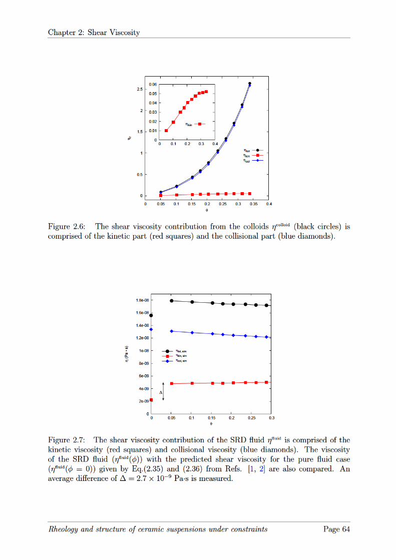
Chapter2:ShearViscosity
0
0.5
1
1.5
2
2.5
0 0.05 0.1 0.15 0.2 0.25 0.3 0.35 0.4
ηr
φ
ηtotηkinηcol
0
0.01
0.02
0.03
0.04
0.05
0.06
0 0.1 0.2 0.3 0.4
ηkin
Figure2.6: Theshearviscositycontributionfromthecolloidsηcolloid
0
2e-09
4e-09
6e-09
8e-09
1e-08
1.2e-08
1.4e-08
1.6e-08
1.8e-08
0 0.05 0.1 0.15 0.2 0.25 0.3
η (Pa • s)
φ
ηtot, simηkin, sim
ηcol, sim
∆
(blackcircles)iscomprisedofthekineticpart(redsquares)andthecollisionalpart(bluediamonds).
Figure2.7: TheshearviscositycontributionoftheSRDfluidηfluidiscomprisedofthekineticviscosity(redsquares)andcollisionalviscosity(bluediamonds). TheviscosityoftheSRDfluid(ηfluid(φ))withthepredictedshearviscosityforthepurefluidcase(ηfluid(φ=0))givenbyEq.(2.35)and(2.36)fromRefs.[1,2]arealsocompared. Anaveragedifferenceof∆=2.7×10⁻⁹Pa·sismeasured.
Rheologyandstructureofceramicsuspensionsunderconstraints Page64

Chapter2:ShearViscosity
sizeeffectsthatmaketheshearratehigherthantheexpectedvalue,thusdecreasingthe
magnitudeofviscosity[31].
TheresultsshownarecomparablewiththoseofKoelmanandHoogerbrugge[4,5],
wheretheysimulatedhard-spheresuspensionsundershearflowusingDPD.Theseare
representedbythehollowtriangles.Thehard-spherecaseisimposedbyusingthemoment
ofinertiaandEuler’sequationofmotionforrigidbodies[5].
Thebehaviourofhard-spheresuspensionsintheabsenceofHIswasanalyzedusing
BDinRef.[3]. TheBDdatapointsarerepresentedbythegreendiamonds.Inorder
toremovePeandvolumefractiondependenciesoftheshearviscosity,Ref.[3]employed
analgorithm,inwhichaftertheBrownianpositionupdates,theoverlapsarechecked
andsuccessivelyremoved[91
0.5
1
1.5
2
2.5
3
3.5
4
4.5
0 0.05 0.1 0.15 0.2 0.25 0.3 0.35 0.4
ηr
φ
SRD-MD (numerical)
BD (numerical)
DPD (numerical)
Segre (experimental)
van der Werff (experimental)
Krieger (analytical)
Einstein (analytical)
]. Bycomparingthebehaviourofthetwosystems,HI’s
increasetheviscosityofthesuspension.IncontrasttotheBDsimulations,wherethe
effectsoffluidparticlesarerepresentedbythefrictionalandstochasticterms,thefluid
descriptioninSRD-MDismoreexplicit.Itisobservedthattheoverallcontributionof
thefluiddecreaseswithincreasingvolumefractionsincethenumberoffluidparticles
decreaseswithincreasingconcentrationtomaintainaconstantScforthefluid. Even
so,thetreatmentofthefluidbySRD-MDprovideslubricationbetweencolloidparticles
becausethefluidcanslidebetweenthem.Thisincreasesthechancesofcollisionsamong
colloidsandtheoverallfrictionofthesystem.
Fromthetheoreticalstandpoint,theresultsfollowEq.(2.37)(greensolidline)forlow
Figure2.8: Relativeshearviscosityofthecolloidalsuspensionasafunctionofvolumefractioncomparedwithothernumerical[3,4,5],experimental[6,7]andanalyticalstudies[8,9,10].
Rheologyandstructureofceramicsuspensionsunderconstraints Page65

Chapter 2: Shear Viscosity
volume fractions and start to diverge near φ = 0.15. For Eq. (2.39) (blue dashed line),
a fitting parameter of φm ∼ 0.74 is used because the highest packing achievable in our
simulation box is hexagonal close packing. Previous theoretical works have shown that
p = 2 for a variety of situations [92, 93] so that Eq. (2.39) reduces to ηr = (1− φ/0.74)−2.
2.5 Conclusions
This chapter has demonstrated that SRD-MD can be used to simulate the shear
viscosity of colloidal suspensions. The mapping between physical and simulated values
can be done by SRD-MD without loosing relevant information. The use of the diffusion
time scale for computation significantly decreases the simulation time. Shear can also be
applied to systems that use MD as a coupling scheme. A Monte Carlo scaling thermostat
is necessary to maintain the correct thermodynamic properties of the fluid.
The choice of σcf = 0.8a in defining the volume fraction also gives the correct viscosity
values because a small σcf allows more fluid particles to perturb the flow field surrounding
the colloid.
The use of stress tensors for viscosity evaluation provides a better characterization
tool than what was previously available as in Ref. [31]. It was observed that the
main contribution to the shear viscosity of the suspension comes from the inter-particle
collisions rather than streaming. The contribution of the fluid particles to the stress
tensor decreases with increasing concentration. This is a consequence of the coupling
scheme used and is necessary in order to preserve the Sc of the fluid. However, their
role in facilitating lubrication between colloidal particles aids in the increase of kinetic
and collisional viscosities of the colloidal suspension, which is not seen in simulations
where hydrodynamics are ignored. The presented results are also comparable with other
experimental and theoretical studies. While results for hard-sphere suspensions employing
other methods, like DPD, have been compared to Eq. (2.37) and (2.39), this is the first
time that the relation between shear viscosity and volume fraction is reproduced with
SRD-MD. Hence this work serves as a final test on the ability of SRD-MD to predict
transport coefficients and rheological parameters where HI’s are significant. Moreover,
in comparison to DPD, the SRD treatment of the system is computationally faster
especially at intermediate and high-volume fractions. This is because it does not rely
on the computation of pair-wise potentials hence the computational cost associated with
additional colloids does not increase significantly. Moreover, since the value of Nf is
reduced at higher concentrations, the number of fluid particles needed to be evaluated is
lowered. SRD-MD is also a practical tool for studying the rheology of dense suspensions,
an important aspect for studying yield-stress and other phenomena that are occurring in
the non-Newtonian regime.
Rheology and structure of ceramic suspensions under constraints Page 66

Chapter 2: Shear Viscosity
This chapter benchmarks SRD-MD in the modeling of HIs in colloidal suspensions.
In the next chapter, SRD-MD is used to determine the effects of HIs in real percolating
alumina systems.
Rheology and structure of ceramic suspensions under constraints Page 67

Chapter 3: Percolation Threshold
Chapter 3 :
Percolation threshold
Rheology and structure of ceramic suspensions under constraints Page 68

Chapter 3: Percolation Threshold
Figure 3.1: Schematic diagram of colloidal clusters in representative simulation boxesthat are (a) not percolating and (b) percolating in 2D.
In this chapter, the percolation phenomenon is modeled using BD and SRD-MD
simulations. Schematic diagrams of non-percolating and percolating systems are shown
in Fig. 3.1. In this figure, colloids are placed in a simulation box with mirror images
to illustrate how percolation is characterized i.e. when the clusters of colloids form a
continuous network that spans through space.
Percolation is a common occurrence in nature and its onset, known as percolation
threshold φc, covers a vast number of fundamental problems in the study of phase
behaviour, structural stability and rheology of complex fluids [94, 95]. Percolation
threshold appears in models concerning gelation [96], glass and phase transition [97, 98]
and conductivity [99] and is therefore of great significance to various industrial and
biological systems. The focus of this chapter is the role of percolation threshold on yield
stress, which will be introduced in the next section. This study is motivated by the fact
that φc appears as a parameter in the mathematical definition of yield stress [22] and is
difficult to evaluate experimentally. To this end, a simulation study can be very helpful.
The range of application of yield stress can start from materials at home like toothpaste
and butter spreads to industry such as paper making, the concrete used for construction
and biological materials including mucus and other relevant problems in biolocomotion
and beyond [98]. Yield stress is also an archetypal rheological property of colloidal
suspensions that is of great importance to several ceramic processes. The goals of this
chapter are as follows: (1) to offer an alternative approach of measuring φc, especially for
systems where experimental methods are limited or difficult to apply; (2) to investigate
the key variables that affect the value of φc namely, attraction strength and hydrodynamic
interactions (HIs); and (3) to compare the results with the yield stress study presented in
Refs. [21, 26].
Rheology and structure of ceramic suspensions under constraints Page 69

Chapter 3: Percolation Threshold
3.1 Yield stress model
For most viscoelastic fluids, yield stress is described as the transition from solid to
fluid behavior. For ceramic suspensions, yield stress is the amount of stress needed to
deform and induce flow to an otherwise mechanically rigid colloidal network [100]. Hence
from the yield stress point of view, one can define the percolation threshold as the point
at which a continuous network of colloids is formed leading to a mechanical resistance to
deformation. The strength of the network dictates the magnitude of yield stress, hence
among the obvious candidates in determining its value are: the density of network of
bonds and the strength interparticle attractions. Since the knowledge of yield stress is
highly beneficial [101, 102, 103], several models have attempted to provide a quantitative
definition of yield stress as a function of these key factors e.g. interparticle forces and
microstructural information [104, 105, 100]. However, the limitation in these models is
that they are often idealized i.e. they lack a clear representation of other important
variables that also contribute to yield stress. This chapter focuses on one important
parameter that is often overlooked in these models i.e. percolation threshold φc.
In their work, Zhou et al. [100] have found that yield stress is dominated by
interparticle forces when φ > φc, and by structural effects of weak links when φ < φc.
While this observation is only qualitative, it explains the deviation of previous theoretical
models from experimental data [100]. This finding clearly indicates that φc needs to be
included in the prediction of yield stress.
Quite recently, a more complete yield stress model (YODEL) that incorporates φc
quantitatively was proposed by Flatt and Bowen [22, 21]. The yield stress τ is given by
τ = m1φ(φ− φc)2
φmax(φmax − φ), (3.1)
where φmax is the maximum packing fraction and m1 is a factor that accounts for particle
size, particle size distribution and interparticle forces. While YODEL shows a good
agreement with experiments, it still uses φc as a fitting parameter.
This drawback mainly stems from the absence of a straightforward experimental
approach that can accurately determine φc. Moreover, the phenomenon itself, despite
its common occurrence, is still poorly understood. To this end, numerical methods can
serve as convenient tool for determining φc and can provide a more detailed investigation
on the variables that may influence its value.
Rheology and structure of ceramic suspensions under constraints Page 70

Chapter 3: Percolation Threshold
3.2 On hydrodynamic effects
HIs are omnipresent in nature and additional insights into the role of HIs in the
aggregation kinetics of colloids have been observed [106, 107, 108]. Hence, even if the
system presented in this chapter is in equilibrium, the presence of HIs can influence the
value of φc. For example, Tanaka and Araki [107] have presented strong indications that
HIs influence the transient gel formation of 2D colloidal particles. One of the reasons is
that a pair of colloids induces a flow field that can rotate another pair of colloids, which
lead to the formation of elongated structures. The other reason is that HIs decrease the
approaching speeds of colloids significantly, which again promotes the formation of open
and chainlike structures.
In constrast, Yamamoto et al. [109] have demonstrated that hydrodynamic effects
have a minor quantitative difference on 3D systems. From their results, hydrodynamic
effects are more noticeable on 2D systems due to finite size effects. However, we note that
their measurements are performed after quenching the system to zero temperature, where
HIs are expected to be negligible [110].
There are other works that supports the preliminary investigations of Tanaka and
Araki for 3D systems. Whitmer and Luijten [110] have studied formation of clusters
at different attraction strengths and have found that, indeed, more elongated clusters
are formed if HIs are considered. However, hydrodynamic effects are outweighed by
interparticle forces when the attraction is strong. Their results have also provided
an additional insight that the effects of hydrodynamics on φc should be investigated
in different regimes of attraction strength. On the other hand, Tomilov et al. [75]
analyzed the aggregation kinetics of colloids by varying the volume fraction and the type
of simulation method. The results provided a new role of HIs i.e. they increase the
diffusion coefficient for aggregates with respect to the value given by Brownian dynamics.
Hence there is a faster cluster-cluster coalescence that impedes the reorganization process
within the aggregate and less compact structures are formed.
While the results from these studies suggest that φc is expected to be lower for a system
with HIs than for that without, the results in Refs. [107, 110, 75] concern 2D systems,
small systems and simple potentials respectively so that the supposed HIs effects on φc
have never been independently verified.
In this chapter, larger 3D systems are used. Derjaguin-Landau-Verwey-Overbeek
(DLVO) theory is also employed and the experimental variables are directly mapped
to simulation parameters thus providing the closest representation of the actual system.
A summary of the work presented in this chapter is published in Ref. [111].
Rheology and structure of ceramic suspensions under constraints Page 71

Chapter 3: Percolation Threshold
3.3 Mapping from physical values to simulation
parameters
The experimental system presented in Ref. [21, 26], where Stuer and Bowen applied
YODEL for doped alumina suspensions, is simulated. The number of spherical colloids
that are suspended in water is fixed to Nc = 500. The density and viscosity of water
is ρf = 1000 kg·m3 and η = 10−3 Pa·s respectively. The system is equilibrated at room
temperature (293 K) using the Monte Carlo thermostat presented in Section 1.5.2. The
colloids have a radius of a = 255 nm. The density of alumina 3300 kg·m3 is so that an
alumina colloid has corresponding mass of M = 2.76×10⁻¹⁶ kg. The suspension is placed
in a simulation box of side length L and periodic boundary conditions are imposed to
model a large percolating system. The value of L is adjusted depending on the volume
fraction φ being studied:
L = 3√
4Ncπa3/(3φ). (3.2)
As in the previous chapter, the number of fluid particles used are decreased for every
volume fraction according to Eq. (1.33). A summary of the volume fractions and of the
corresponding Nf and φ values are shown in Table 3.1.
Table 3.1: Corresponding side length of simulation box (L) and number of fluid particles(Nf ) in terms of colloid radius a for different volume fractions (φ).
φ(%) 6 7 8 9 10L/a0 65 62 59 57 55Nf 1330232 1148747 984002 883072 788982
φ(%) 11 12 13 14 15L/a0 53 52 51 49 48Nf 701492 660147 620362 545352 510067
The colloid-fluid is modeled by the IP potential presented in the previous chapter (Eq.
1.31). For the colloid-colloid interaction, the DLVO theory is utilized because it is the
closest approximation to real colloidal systems. The DLVO theory, which was developed
in the 1940’s by Derjaguin and Landau [17] and Verwey and Overbeek [18], has been
featured prominently in several studies. Its ability to predict the stability of the colloids
suspended in fluid has been crucial for the advancement of colloidal science. In the DLVO
theory formulation, the total interaction is the sum of two contributions: the attraction
due to van der Waals forces U vdWij ; and electrostatic repulsion U el
ij due to the double layers
formed by surface charges:
UDLVO
ij = U vdW
ij + U el
ij. (3.3)
The interaction strength depends on the dielectric properties of both the colloids and the
Rheology and structure of ceramic suspensions under constraints Page 72

Chapter 3: Percolation Threshold
fluid. The van der Waals term is always attractive and follows a power-law dependence.
For particles of the same radius a, this is given by:
U vdW
ij = −A6
{2a2
r2ij − (2a)2
+2a2
r2ij
+ ln
[r2ij − (2a)2
r2ij
]}. (3.4)
Here, rij is the center-to-center distance between particles i and j and A = 4.76× 10⁻²⁰ J
is the Hamaker constant for alumina in water [37, 112]. For the electrostatic repulsion
part, the Hogg-Healy-Fuerstenau equation is used:
U el
ij = πεaψ2
{ln
[1 + e−κd
1− e−κd
]+ ln
[1− e−2κd
]}, (3.5)
where d = rij − 2a, ε = 81ε0 is the dielectric constant of water, ε0 is the permittivity of
free space, ψ = 100 mV is the surface potential and κ is the inverse of the Debye screening
length given by
κ =
√e2
εkBT
∑k
nkz2k, (3.6)
where e is the elementary electronic charge; and nk and zk are the volume density and
valency of ion k respectively. A summary of the parameters used is listed in Table 3.2.
Table 3.2: Parameters used in the study of Percolation.
M 2.76× 10⁻¹⁶ kg a 255 nm ψ 100 mVA 4.76× 10⁻²⁰ J ε 81ε0 T 293 K
One of the points raised in Ref. [21] is the effect of κ on φc:
κ =
√e2
εkBT
∑k
nkz2k, (3.7)
where e is the elementary electronic charge; and nk and zk are the volume density and
valency of ion k respectively.
The values of κ that are used in this work are shown in Fig. 3.2. Modifying κ effectively
changes the attraction strength between the alumina particles. It is important to note
that in this system, the aggregation is not caused by the first deep minimum since the
colloids would have to overcome a very high potential barrier (≈ 1200kBT ) to reach that
first minimum (see Fig. 3.2 ). Instead, the aggregation is caused by the trapping in the
secondary minimum, whose depth can be modulated by varying κ (see inset of Fig. 3.2).
BD simulations for different values of κ corresponding to potential well depths of 10kBT ,
7kBT , 5kBT and 4kBT are performed. In the case of SRD-MD simulations, well depths of
10kBT and 5kBT are considered. These well depths of the secondary minima are typical
Rheology and structure of ceramic suspensions under constraints Page 73

Chapter3:PercolationThreshold
0
200
400
600
800
1000
1200
1400
510 520 530 540 550
UijDLVO ( kBT )
rij ( nm )
-10
-5
0
5
10
520 560 600 640
κ = 0.2803 nm-1
κ = 0.3195 nm-1
κ = 0.3924 nm-1
κ = 0.4932 nm-1
Figure3.2: TheDLVOpotentialfordifferentvaluesofinverseDebyescreeninglengthκ.Inset:theattractionstrengthbetweenthecolloidsvarywiththewelldepthofthesecondaryminimum.
forthealuminasystemstudiedinRef.[21,26]forionicconcentrationsofbetween2-5
mMforMgandYnitrates. Thesearetypicalconcentrationsfordopantlevelsof250-
500ppmtypicallyusedintheproductionofpolycrystallinealuminas[26].
Togetacompleteunderstandingofφc,anaccuraterepresentationofHIsinpercolating
systemsisnecessary.ThechallengeonthecomputationalcostofmodelingHIsremains.
Sincemostpercolatingsystemsarelargesystems,computationalefficiencyisvital. To
thisendSRD-MDishighlysuitableforthestudyofpercolation.Hydrodynamiceffects
areisolatedbycomparingthesimulationresultsofSRD-MDwiththeBDresults.
3.4 Timescales
FollowingtherecipesofRef. [31]instudyingcolloidalsuspensionswithDLVO
potential,thetimescalesarecheckedfor255-nmaluminacolloids. Thephysicaltime
scalesandthecorrespondingcoarsegrainedtimescalesareshowninTable3.3. The
variableτ0correspondstotheoscillationfrequencyatthebottomofthesecondminimum
[65]. Notethattheorderingofthetimescalesi.e.τD >τ0>τv>τB inthephysical
regimeisthesameastheorderingoftimescalesintheSRD-MDregime. Thismeans
thatthephysicalbehaviourofthecolloidsispreservedwhenobservingatthediffusion
timescale[31,30].
ThetimestepusedforBDis∆tBD =2×10⁻⁷s.FortheSRD-MDsimulations,the
sameframeworkasdiscussedinChapter3isused.ThetimescaleforSRD-MDischosen
Rheologyandstructureofceramicsuspensionsunderconstraints Page74

Chapter 3: Percolation Threshold
Table 3.3: Hierarchy of time scales for a 255-nm alumina colloid suspended in water andits corresponding coarse grained values for SRD-MD.
τD τ0 τν τBPhysical 1.5× 10⁻¹ 2.5× 10⁻⁴ 1.3× 10⁻⁷ 5.7× 10⁻⁸
SRD-MD 1.5× 10⁻¹ 8.9× 10⁻² 9.2× 10⁻³ 7.1× 10⁻³
Table 3.4: SRD parameters used in the study of percolation threshold.
α 90◦ σ 204 nmγ 5 TSRD 0.002 Kλ 0.1 ∆tSRD 4.53× 10⁻⁵ sa0 127.5 nm mf 4.145× 10⁻¹⁹ kg
so that the most relevant time scale for percolation analysis, i.e. the colloid diffusion time
τD, is accurately reproduced. The experimental value of τD is 1.5 × 10⁻¹ s. For the MD
part, an MD time step of ∆tMD = 18∆tSRD = 5.67 × 10⁻⁶s is chosen. Consequently, the
SRD temperature becomes TSRD = 0.002 K and the units of energy and viscosity of the
simulation changes to kBTSRD = 2.8×10⁻²⁶ and ηSRD = 1.76×10⁻⁸ Pa·s respectively. The
value of ηSRD is computed using the analytical equation for fluid viscosity that is presented
in Sec. 2.2.3. The SRD parameters employed in this study are summarized in Table 3.4.
3.5 Parameters for aggregate analysis
One can describe a percolating system as being made up of aggregated colloids, where
the largest aggregate spans an infinitely large space. Hence the first step into quantifying
the aggregation kinetics is to provide a definition of an aggregate. In the simulations, an
aggregate is an assembly of two or more connected colloids. Two colloids are considered as
being connected when their mutual distance rij ≤ δr, where δr/2 = 1.2a = 306 nm. The
value of δr corresponds to the first-neighbor distance obtained from the radial distribution
function of the aggregated system. A schematic diagram is shown in Fig. 3.3
3.5.1 Number of aggregates vs time (NA vs t)
From Ref. [75], it has been shown that the aggregation process can be divided into
three regimes. The first is dimer formation, where solitary colloids pair up with other
colloids. The second is aggregate coalescence, where aggregates come together to form
larger clusters. The final step, which is reorganization, happens when the attraction
strength permits detachment and re-attachment within the aggregate that promotes
ordering. These regimes can be observed by monitoring the number of aggregates NA as a
function of time. The result of the time evolution NA can also determine the appropriate
Rheology and structure of ceramic suspensions under constraints Page 75

Chapter 3: Percolation Threshold
Figure 3.3: The value of δr dictates whether the nearest colloid is a considered asneighbor or not.
time interval for the measurement of φc.
3.5.2 Parameters PD and φc
To numerically pinpoint φc, the same process used in Ref. [38] is employed. From the
original simulation box of side length L, seven other mirror images are produced in the
x, y and z directions, resulting to a larger box with size of 2L× 2L× 2L. Once the new
box is formed, the largest aggregate traversing the enlarged box is singled out and its
linear extensions (Dx, Dy, Dz) along the three directions are measured. If the components
of D satisfy the condition:
Di ∈ [2L− δr, 2L], where i = x, y, z (3.8)
then the aggregate is counted as percolating in the ith direction. To characterize the
type of percolation in a system i.e. in 1 direction, in 2 directions or in all 3 directions,
the number of times Eq. (3.8) is satisfied is recorded for a given volume fraction. This
dimensionless parameter is called PD. The results reported here are averaged over 5
independent simulations so that PD can have non-integer values between 0 and 3. For
example, if for a given volume fraction, 3 simulations percolate in 3 directions and the
other two simulations percolate in 1 direction, then the resulting PD is 2.2. The value of
PD also represents the probability of observing percolation in 3 directions.
To characterize φc and to account for the statistics of 5 different simulations, a
threshold for PD is set. Specifically, φc is determined by the conditions that for
φ = φc, PD > 2 and for all φ > φc, PD ≥ 2. If PD ≥ 2 the average percolation is in
at least 2 directions. This means that at least one of the simulations fully percolates in 3
directions. Choosing a lower threshold for PD would not change the qualitative trends of
the results, while somewhat decreasing the values of φc, especially for the cases of weaker
Rheology and structure of ceramic suspensions under constraints Page 76

Chapter 3: Percolation Threshold
attraction. It is also important to note that if PD = 1 is chosen instead of PD = 2,
the results would be noisier because they are related on average to system with fewer
particles.
3.5.3 Number of nearest neighbors
Systems with elongated aggregates tend to have higher values of PD. Consequently,
the values of φc for these systems are expected to be low. Hence the values of PD and
φc can already characterize the systems between having elongated aggregates or compact
aggregates. However, a different method of quantifying the ordering of an aggregate can
also be performed independently. This is done by counting the percentage of colloids
having 12 nearest neighbors [113]. Since compactness is correlated to the degree of
organization, it is expected that compact aggregates have higher percentages of nearest
neighbors than their elongated counterparts.
3.6 Results
3.6.1 Dissociation times
The reorganization process is a consequence of the dissociation and association of the
colloids within an aggregate. The frequencies of dissociation and association of colloids
dictate the amount of ordering an aggregate can achieve, which can affect the value of φc.
The challenge in SRD-MD is that only one time scale can be accurately reproduced during
the mapping procedure. The rest of the time scales will have values that are different from
the experimental values. As mentioned in Ref. [30], the correct physics is still reproduced
as long as the ordering of the time scales is preserved (see Table 3.3). However, it still
important to check the dissociation time scale of the percolating system presented in this
chapter to ensure that the reorganization of the colloids is not affected by the mapping
procedure of SRD-MD. Note that a similar problem is not present in the BD simulations.
The dissociation time is tested using the DLVO potential with a well depth of 7kBT .
This value was chosen because it lies in the middle of 10kBT and 5kBT . Moreover, a
simulation for a 10kBT potential well depth is time consuming while a simulation for a
5kBT potential well depth is too fast so that it is prone to statistical errors. To determine
an average dissociation time, two colloids are placed in a simulation box (L = 32a0)
at an equilibrium distance r0 = 5.29264 × 10⁻⁷ m and are allowed to evolve until they
dissociate at time τdissoc. The calculated values are shown in Table 3.5. The reported values
are averaged over 200 independent simulations. The results show that the dissociation
time for SRD-MD is longer than the dissociation time for BD. This is expected because by
Rheology and structure of ceramic suspensions under constraints Page 77

Chapter 3: Percolation Threshold
Table 3.5: Dissociation times for BD and SRD-MD.BD SRD-MD
∆t (s) 2.0× 10⁻⁷ 4.53× 10⁻⁵
τdissoc (s) 0.22 0.68
0
1
2
3
4
5
0 1 2 3 4 5
% o
f col
loid
s w
ith 1
2 ne
ares
t nei
gbor
s
Time (s)
Diffusion timeDissociation time
Figure 3.4: The degree of ordering for a 5kBT well, measured by the percentage ofcolloids having 12 nearest neighbours. This is a comparison between the diffusion timescale (∆tSRD = 4.53×10⁻⁵ s) and dissociation time scale (∆tSRD = 2×10⁻⁵ s). The systemconsists of 200 colloids in a dilute environment of φ = 5%. The results are averaged over5 simulations.
mapping to the diffusion time scale, the rest of the time scales, including the dissociation
time scale, will have values that are different from the experimental or BD values.
Hence to see if the difference in dissociation times affects the reorganization of the
aggregate, two types of simulations are performed: one mapped to the diffusion time scale
(∆tSRD = 4.53×10⁻⁵ s); and the other map to the dissociation time scale (∆tSRD = 2×10⁻⁵
s). The system used consists of 200 colloids in a dilute environment (φ = 5%). A well
depth of 5kBT is used because the ordering for the 7kBT and 10kBT systems are not
recognizable for the simulation time that is achievable (≈ 5 s). The results in Fig 3.4
show that the difference between the reorganization of the clusters is not significant even
if the dissociation times are different. Therefore, even with the mapping procedure used
in SRD-MD, the ordering of the colloids is properly reproduced.
3.6.2 Influence of the colloid-colloid attraction strength
Before analyzing the simulation results, a preliminary check of the appropriate time
interval needed to obtain a stationary state is necessary. This is important because
Rheology and structure of ceramic suspensions under constraints Page 78

Chapter 3: Percolation Threshold
1
10
100
NA
5 kBT w/ HIs
5 kBT w/o HIs
1
10
100
1 2 3 4 5
NA
t (s)
10 kBT w/ HIs
1 2 3 4 5t (s)
10 kBT w/o HIs
15%14%13%
12%11%10%
9%8%7%
Figure 3.5: Semi-logarithmic plot of the number of aggregates NA vs time t for potentialwell depths 5kBT and 10kBT for different volume fractions.
Rheology and structure of ceramic suspensions under constraints Page 79

Chapter3:PercolationThreshold
aggregatecoalescenceisslowerintheabsenceofHIs[75]anditisimportanttohave
approximatelythesamesizesofaggregateswhendeterminingφc.Sampleresultsofthe
temporalevolutionofthenumberofaggregatesNAfor5kBTand10kBTcasesareshown
inFig.3.5.Sincetheformationofalargeaggregate,theoneresponsibleforpercolation,is
fasterwithHIs,thePDoftheaggregatesformedat5swhenHIsarepresentarecompared
tothePDoftheaggregatesformedat5sand20swhenHIsareabsent.At20s,theNA
valuesarealmostthesamebetweenthetwosimulations.
ForthesystemswithoutHIs,themeasuredPD valuesfordifferentvolumefractions
areshowninFigs.3.6.Byimposingthelimitthattheonsetofpercolationhappenswhen
PD>2,thefollowingφcforthedifferentwelldepthsareobtained:15%for4kBT,12%for
5kBT,9%for7kBTand8%for10kBT.Sincetherearenosignificantdifferencesbetween
thevaluesofPD measuredat5sand20s,theφc
0
1
2
3
PD
(a) after 5s
0
1
2
3
6 7 8 9 10 11 12 13 14 15 16
PD
φ (%)
(b) after 20s
4 kBT 5 kBT 7 kBT 10 kBT
valuesdonotchangebetweenthetwo
timeintervals.Itisnotablefromtheseresultsthatthepercolationthresholdisgreatly
Figure3.6: ThenumberofdirectionsthesystemispercolatingPDisplottedagainstthevolumefractionφforsytemswithoutHIs. Therearenosignificantdifferencesbetweenthemeasurementsdoneafter5sand20s.
Rheologyandstructureofceramicsuspensionsunderconstraints Page80
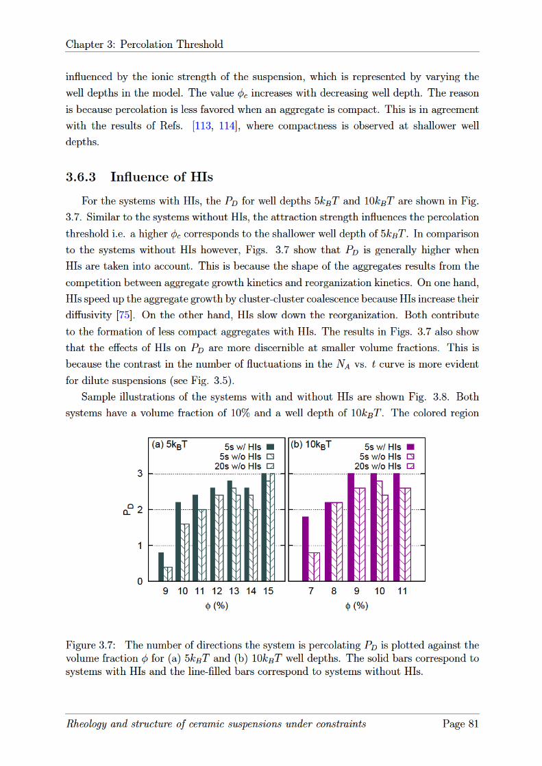
Chapter3:PercolationThreshold
influencedbytheionicstrengthofthesuspension,whichisrepresentedbyvaryingthe
welldepthsinthemodel.Thevalueφcincreaseswithdecreasingwelldepth.Thereason
isbecausepercolationislessfavoredwhenanaggregateiscompact.Thisisinagreement
withtheresultsofRefs.[113,114],wherecompactnessisobservedatshallowerwell
depths.
3.6.3 InfluenceofHIs
ForthesystemswithHIs,thePD forwelldepths5kBTand10kBTareshowninFig.
3.7.SimilartothesystemswithoutHIs,theattractionstrengthinfluencesthepercolation
thresholdi.e.ahigherφccorrespondstotheshallowerwelldepthof5kBT.Incomparison
tothesystemswithoutHIshowever,Figs.3.7showthatPD isgenerallyhigherwhen
HIsaretakenintoaccount.Thisisbecausetheshapeoftheaggregatesresultsfromthe
competitionbetweenaggregategrowthkineticsandreorganizationkinetics.Ononehand,
HIsspeeduptheaggregategrowthbycluster-clustercoalescencebecauseHIsincreasetheir
diffusivity[75]. Ontheotherhand,HIsslowdownthereorganization.Bothcontribute
totheformationoflesscompactaggregateswithHIs.TheresultsinFigs.3.7alsoshow
thattheeffectsofHIsonPD aremorediscernibleatsmallervolumefractions. Thisis
becausethecontrastinthenumberoffluctuationsintheNAvs.tcurveismoreevident
fordilutesuspensions(seeFig.3.5).
SampleillustrationsofthesystemswithandwithoutHIsareshownFig.3.8.Both
systemshaveavolumefractionof10%andawelldepthof10kBT
0
1
2
3
9 101112131415
PD
φ (%)
(a) 5kBT 5s w/ HIs5s w/o HIs20s w/o HIs
7 8 9 10 11
φ (%)
(b) 10kBT 5s w/ HIs5s w/o HIs20s w/o HIs
.Thecoloredregion
Figure3.7: ThenumberofdirectionsthesystemispercolatingPDisplottedagainstthevolumefractionφfor(a)5kBTand(b)10kBTwelldepths.ThesolidbarscorrespondtosystemswithHIsandtheline-filledbarscorrespondtosystemswithoutHIs.
Rheologyandstructureofceramicsuspensionsunderconstraints Page81

Chapter 3: Percolation Threshold
represents the largest aggregates formed. In the case shown here, it is apparent that the
largest aggregate in the system with HIs is more elongated. The biggest aggregate, when
there are no HIs present, is percolating in only 1 direction; while the biggest aggregate,
when HIs are present, is percolating in all 3 directions.
Figure 3.8: A system without HIs simulated using BD (left) vs. a system with HIssimulated using SRD-MD (right). The colored region represents the largest aggregateformed. By comparison, the aggregate simulated with HIs is more elongated and has ahigher probability of percolating than the aggregate simulated without HIs.
3.6.4 Percolation threshold measurements
Here, the PD > 2 condition is considered as a criterion to define the onset of
percolation. The observed elongation of aggregates induces some decrease in the measured
φc. This decrease is more evident when the potential well is shallow. In fact, φc = 8%
is obtained for the 10kBT potential well, regardless of HIs effects, even though the result
for φ = 7% with HIs is very close to verify the PD > 2 condition. On the other hand,
φc = 10% with HIs and φc = 12% without HIs for the 5kBT potential well.
The fluctuations of NA during the aggregation process help in understanding whether
hydrodynamic effects are more important at shallower well depths. The results are
presented in Fig. 3.5. The fluctuations in the curve correspond to the association and
dissociation of aggregates that promotes reorganization. Indeed the fluctuations are more
prevalent without HIs and this difference is more recognizable in the 5kBT case than in
the 10kBT case.
To further verify the compactness of the system, the number of neighbors is used as an
order parameter. Fig. 3.9 shows the percentage of colloids having 12 nearest neighbors as
Rheology and structure of ceramic suspensions under constraints Page 82

Chapter 3: Percolation Threshold
a function of time for the 5kBT well. The corresponding plots for the 10kBT systems are
essentially zero and are not shown here. Note that the variations of the order parameter
as a function of volume fraction are within statistical errors. Hence only the average
differences between systems with and without HIs are considered. Since the percentage
of colloids having 12 nearest neighbors is lower with HIs, this justifies that the structures
obtained after 5 s are more elongated when HIs are accounted for.
0
1
2
3
4
5
6
7
8
0 1 2 3 4 5
% o
f col
loid
s w
/ 12
near
est n
eigh
bors
t (s)
w/ HIs9%
10%11%12%13%14%15%
0 1 2 3 4 5t (s)
w/o HIs9%
10%11%12%13%14%15%
Figure 3.9: The rate of ordering for 5kBT measured by counting the number of colloidswith 12 nearest neighbours. The system without HIs shows a higher degree of ordering incomparison to the system with HIs. For 10kBT , this order parameter is essentially zero.
These observations suggest that for high ionic strengths, the attraction strength
dictates the value of φc since it dominates over the effects of HIs. However, for low
ionic strengths, HIs influence φc by lowering its value. The kinetics plays a crucial role in
dictating φc. Aggregation is a three-part process: dimer formation, aggregate coalescence,
reorganization. The first two stages are studied in Ref. [75]. However, it is worth noting
that there is an overlap in the aggregate coalescence and reorganization stages. The
combination of the fast aggregate coalescence with the slow reorganization due to HIs
both affect φc.
The results of the simulations are summarized in Fig. 3.10. The solid line dividing the
two regions is an approximate φc value when HIs are not present. The shaded region
corresponds to a higher probability of observing percolation in 3D. The red squares
represent φc values measured when HIs are included. When comparing the simulation
results with the results of the yield stress modeling in Refs. [21, 26], a good correspondence
with BD simulations is found for the higher ionic strengths of 0.0044 M (Y 3+), where the
Rheology and structure of ceramic suspensions under constraints Page 83

Chapter 3: Percolation Threshold
6
7
8
9
10
11
12
13
14
15
4 5 6 7 8 9 10
Vol
ume
Frac
tion
(%)
Potential well depth (kBT)
w/ HIs (SRD-MD)w/o HIs (BD)
Y3+ 0.0044 M (YODEL)Mg2+ 0.0078 M (YODEL)Mg2+ 0.0044 M (YODEL)
Figure 3.10: The summary of percolation threshold for systems with and without HIspresented as a relation between potential well depth and volume fraction.
well depth was around 6.4kBT and φc = 10%. On the other hand, the estimated φc are
12% and 14% for the shallower well depths of 4.67kBT and 3.6kBT respectively. These
values are lower than the ones predicted by BD. However, this is still in good agreement
with the simulation results since a shift to smaller values is expected for shallower well
depths as a consequence of introducing HIs. Moreover, in Refs. [21, 26] the estimate of
φc follows from a fitting procedure within the YODEL model.
3.7 Conclusions
In conclusion, the results show that stronger interparticle attractions decrease the
magnitude of the percolation threshold φc. In addition to this, higher PD values
are observed when HIs are present due to the more elongated structures formed.
Correspondingly, an effect of HIs on the percolation threshold is seen. This effect is
evident for shallow potential wells (φc = 10% with HIs and φc = 12% without HIs for a
well depth of 5kBT ), and tends to become smaller and smaller with increasing well depth.
It is important to note that the simulation measurements are performed at specific time
intervals. The transient aggregates observed may evolve to stable low-energy structures
[109] or arrested structures [115, 23, 116, 117]. But the time scale to which this may occur
and the final state of the aggregate is difficult to predict. Despite this, a good qualitative
agreement between simulations and experiments is observed.
Finally, the results of this chapter can also be used to determine the most convenient
Rheology and structure of ceramic suspensions under constraints Page 84

Chapter 3: Percolation Threshold
simulation method for studying percolation in colloidal aggregates. A good indicator for
determining the most appropriate method is the attraction strength between the colloids.
When the attraction is strong (well depths of 10kBT or more), the rearrangement is
very slow due to the high energy barriers hindering the motion of colloids inside the
aggregates. This is the dominating factor for determining the percolation threshold,
while hydrodynamic effects tend to be negligible. In this case, BD simulations, which are
considerably faster than any other method with HIs, should suffice. These general trends
are also in good agreement with estimates of the percolation threshold for the deeper well
depths from yield stress modeling using YODEL. On the other hand, for weaker colloid-
colloid attraction, hydrodynamic effects on percolation can be sizable, so that methods
which include HIs should be used. In this case, it is worth noting that SRD-MD is still
the fastest technique available that can model HIs in percolating networks.
In the next chapter, BD simulations are performed to investigate the aggregation
of colloidal suspensions on attractive walls. BD simulations are used because they are
simpler and relatively well-known for the system being modeled. Additionally, an initial
study for shaken colloidal suspensions is performed. The same alumina system discussed
in this chapter in placed under an oscillating shear force to determine whether it can
enhance the ordering of the aggregates.
Rheology and structure of ceramic suspensions under constraints Page 85

Chapter 4: Attractive Walls and Shaking
Chapter 4 :
Attractive Walls and Shaking
Rheology and structure of ceramic suspensions under constraints Page 86

Chapter 4: Attractive Walls and Shaking
The ability to tune the interaction between particles in the presence of external forces
is a quintessential problem in colloidal science [118, 119, 120]. The presence of a solid
surface and/or external shear are more common in experiments than the occurrence of
a perfect system without any external perturbation. From a theoretical point of view,
this type of problem is also interesting because it can provide additional insights not just
about the actual motion of colloids in the fluid, but also about the mechanisms that rule
colloid aggregation with external forces. Moreover, this work can be potentially useful
in designing experimental procedures that can be used to obtain crystals with desired
structures and properties.
4.1 Attractive Walls
Particular attention has been given to the numerical modeling of the aggregation of
colloids [19, 16]. As mentioned, the primary reason is because colloids display the same
phase behavior as atoms and molecules, but with the mesoscopic size advantage thus
allowing direct obervation in real space [121, 122]. Another reason is because colloids
serve as excellent models in the understanding of protein adsorption on surfaces since
both systems are subject to the same thermodynamics, but with the colloids having the
benefit of simpler length scales [119, 123]. Therefore, whether the problem is on protein
adsorption [124] or the efficacy of deposition in implant materials [125], a predictive
model that can explain the behavior and properties of colloids can be used to increase
our understanding of the aggregation kinetics of the colloidal particles.
In this chapter, binary colloidal suspensions are used. These are systems consisting of
two types of particles, which can acquire opposite charges in the suspension and interact
mainly through screened electrostatic forces. Binary systems have been prominently
Figure 4.1: Sample primitive cells for NaCl-type lattices (left) and CsCl-type lattices(right). For the NaCl lattice, an atom is surrounded by 6 first nearest neighbors of adifferent kind. For the CsCl lattice, an atom is surrounded by 8 first nearest neighbors ofa different kind.
Rheology and structure of ceramic suspensions under constraints Page 87
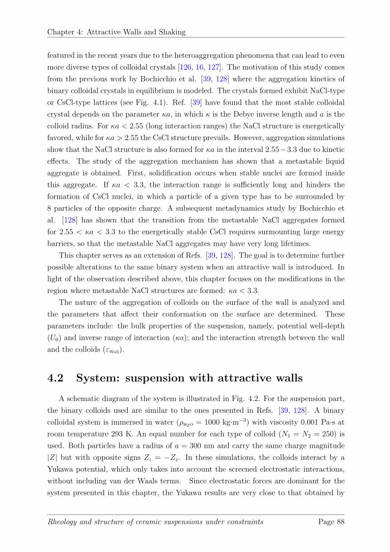
Chapter 4: Attractive Walls and Shaking
featured in the recent years due to the heteroaggregation phenomena that can lead to even
more diverse types of colloidal crystals [126, 16, 127]. The motivation of this study comes
from the previous work by Bochicchio et al. [39, 128] where the aggregation kinetics of
binary colloidal crystals in equilibrium is modeled. The crystals formed exhibit NaCl-type
or CsCl-type lattices (see Fig. 4.1). Ref. [39] have found that the most stable colloidal
crystal depends on the parameter κa, in which κ is the Debye inverse length and a is the
colloid radius. For κa < 2.55 (long interaction ranges) the NaCl structure is energetically
favored, while for κa > 2.55 the CsCl structure prevails. However, aggregation simulations
show that the NaCl structure is also formed for κa in the interval 2.55−3.3 due to kinetic
effects. The study of the aggregation mechanism has shown that a metastable liquid
aggregate is obtained. First, solidification occurs when stable nuclei are formed inside
this aggregate. If κa < 3.3, the interaction range is sufficiently long and hinders the
formation of CsCl nuclei, in which a particle of a given type has to be surrounded by
8 particles of the opposite charge. A subsequent metadynamics study by Bochicchio et
al. [128] has shown that the transition from the metastable NaCl aggregates formed
for 2.55 < κa < 3.3 to the energetically stable CsCl requires surmounting large energy
barriers, so that the metastable NaCl aggregates may have very long lifetimes.
This chapter serves as an extension of Refs. [39, 128]. The goal is to determine further
possible alterations to the same binary system when an attractive wall is introduced. In
light of the observation described above, this chapter focuses on the modifications in the
region where metastable NaCl structures are formed: κa < 3.3.
The nature of the aggregation of colloids on the surface of the wall is analyzed and
the parameters that affect their conformation on the surface are determined. These
parameters include: the bulk properties of the suspension, namely, potential well-depth
(U0) and inverse range of interaction (κa); and the interaction strength between the wall
and the colloids (εWall).
4.2 System: suspension with attractive walls
A schematic diagram of the system is illustrated in Fig. 4.2. For the suspension part,
the binary colloids used are similar to the ones presented in Refs. [39, 128]. A binary
colloidal system is immersed in water (ρH2O = 1000 kg·m−3) with viscosity 0.001 Pa·s at
room temperature 293 K. An equal number for each type of colloid (N1 = N2 = 250) is
used. Both particles have a radius of a = 300 nm and carry the same charge magnitude
|Z| but with opposite signs Z1 = −Z2. In these simulations, the colloids interact by a
Yukawa potential, which only takes into account the screened electrostatic interactions,
without including van der Waals terms. Since electrostatic forces are dominant for the
system presented in this chapter, the Yukawa results are very close to that obtained by
Rheology and structure of ceramic suspensions under constraints Page 88

Chapter 4: Attractive Walls and Shaking
Figure 4.2: Schematic diagram of the walled system. The attractive wall with varyingwell-depth is placed at rz = 0 and a neutral wall is placed at rz = L to avoid particlesfrom reaching heights that are very far from the attractive wall.
Table 4.1: Parameters for system with attractive walls
Nc 500a 300 nmε 81ε0∆tBD 2× 10⁻⁷ sTBD 293 K
Rheology and structure of ceramic suspensions under constraints Page 89

Chapter 4: Attractive Walls and Shaking
the more sophisticated DLVO potential. For particles with equal radii a, the Yukawa
potential is given by
UYij =
ZiZj(1 + κa)2
e2
4πε
e−κ(rij−d)
rij(4.1)
where Zi and Zj are the charges of particles i and j respectively, e is the elementary
electron charge, rij is the center to center distance between particles i and j, and d =
2a = 600 nm. The dielectric constant of water is ε = 81ε0, where ε0 is the permittivity
of free space. The term κa is an important physical parameter that describes the length
scale of electrostatic interactions relative to the particle radius. A lower κa value means a
longer range of repulsion while a higher κa value means a shorter range of repulsion. Since
it was found in Ref. [39] that NaCl structures are formed when κa < 3.3, the focus of this
work is in this region of interaction ranges. The following values of κa = 3, 2.55, 1.5 and
1 are tested against the strength of interaction with the attractive wall. Fig. 4.3 shows
an example of Yukawa potential interaction colloids in the suspension. In this example,
the inverse Debye screening length used has a value of κ = 0.00831 nm−1 and the charges
used have a magnitude of |Z| = |251|.The interactions between oppositely charged colloids are attractive and diverge as
rij → 2a. To avoid numerical instabilities associated with this asymptotic behavior, the
hard-wall potential given by
UHWij =
(rij − 2Bija
Cij
)4
−Dij (4.2)
is connected to the Yukawa potential. Dij has units of energy and regulates the depth of
the well. The parameters Bij and Cij are dimensionless parameters that can be chosen
such that:
Bij =1
2a
{r′ − 4
[Uij(r) +Dij
dUij(r)/dr
]}(4.3)
Cij = 4[Uij(r) +Dij]
3/4
dUij(r)/dr(4.4)
where r′ is the point of connection. Another alternative is to use a linear function that
directly cuts the DLVO or Yukawa potential at a desired distance. However Eq. (4.2)
gives a continuous function for the equations of the potential and the force thus allowing
smooth transition between the attractive and repulsive part. A continuous first and second
derivative means that instabilities in the simulation can also be avoided. For the example
shown in Fig. 4.3, the cut-off distance for the attractive interactions is set to 1.072d while
the cut-off distance for the repulsive interactions is set to 1.02d [128].
To describe the attractive surface, a simple potential in the form of the Lennard-Jones
Rheology and structure of ceramic suspensions under constraints Page 90

Chapter 4: Attractive Walls and Shaking
-20
-15
-10
-5
0
5
10
15
20
1 1.1 1.2 1.3 1.4 1.5 1.6 1.7 1.8
UijY
uk (
k BT
)
rij/a
AttractiveRepulsive
Figure 4.3: The interaction between alumina and silica colloids in the suspension isdescribed by a Yukawa potential with parameters listed in Table 4.1.
Table 4.2: The well-depth values of the LJ 9-3 potential that used to define the interactionof the colloids with the wall. The effective potential well-depth is given by εWall.
εWall (kBT ) εWall(kBT )8 0.099509 0.11200
10 0.1244011 0.1368012 0.1499015 0.18700
(LJ) 9-3 potential is used:
UWall(r) =2
3πρWallσ
3wallεWall
(2
5
σ9Wall
r9z
− σ3Wall
r3z
), (4.5)
where ρWall = 5 and σWall = 4a. Note that simulations with σWall = 1.2a are also checked
and similar results to σWall = 4a are obtained. The value of εWall is varied to modulate the
strength of attraction between the walls and the colloids. The effective potential well is
given by the terms outside the parentheses: εWall = 23πρσ3εWall. A list of the values used
are shown in Table 4.2.
The surface of the wall is at rz = 0 and the first layer of colloids are formed around
3.1 < rz < 3.5. A neutral wall is placed at rz = L to avoid particles from reaching
heights far from the attractive surface. Hence the system is periodic only in the x and y
directions.
Rheology and structure of ceramic suspensions under constraints Page 91

Chapter 4: Attractive Walls and Shaking
The suspensions are relatively dilute with a volume fraction of φ = 20% so that HIs
are expected to be significantly small. The simulations are performed using the Brownian
Dynamics algorithm in GROMACS [129] with a time step of ∆tBD = 2× 10⁻⁷ s.
4.3 Parameters for Aggregate Analysis
P3D is a parameter that can be used to discriminate the formation of either NaCl-type
or CsCl-type lattices. This is defined as follows [39]:
P3D =1
Nc
∑i6=j
[1
12exp
(rij − rNaCl
2σ2NaCl
)− 1
6exp
(rij − rCsCl
2σ2CsCl
)]. (4.6)
The first term corresponds to the probability of finding a particle with 12 second nearest
neighbors (SNN) around a cut-off radius of rNaCl = 895 nm. The second term corresponds
to the probability of finding a particle with 6 SNN around a cutoff radius of rCsCl = 737
nm. The values of rNaCl, rCsCl and their corresponding standard deviations σNaCl = 20
nm and σCsCl = 20 nm are obtained from the radial distribution function of the colloids
[27]. As a further verification step, a two-dimensional version of Eq. (4.6) is used. It was
observed that the first layer of CsCl and NaCl attached to the surface of the wall can be
differentiated. A CsCl structure will have its (101) plane attached to the surface of the
wall while an NaCl structure will have its (100) plane attached to the surface wall. The
(101) CsCl-plane leads to a rectangular lattice with one side having rCsCl while the (100)
NaCl-plane leads to a square lattice with rNaCl. In 2D, the SNN for CsCl with rCsCl is 2;
while the SNN for NaCl with rNaCl is 4. Taking this into consideration, the parameter P2D
is defined as follows:
P2D =1
Ns
∑i6=j
[1
4exp
(rij − rNaCl
2σ2NaCl
)− 1
2exp
(rij − rCsCl
2σ2CsCl
)], (4.7)
where Ns is the total number of colloids on the surface.
4.4 Results
4.4.1 NaCl vs CsCl
First, the effect of the wall on a suspension is analyzed. For this part, a system
with U0 = 9kBT and κa = 2.55 is used as an example. In an infinite system, the
expected final structure for this suspension is NaCl. Fig. 4.4 shows what happens to
the suspension when a wall with εWall = 10kBT is introduced. In the beginning of the
Rheology and structure of ceramic suspensions under constraints Page 92

Chapter 4: Attractive Walls and Shaking
Figure 4.4: Snapshot of the suspension with U0 = 9kBT , κa = 2.55 and ε = 10kBT att = 1.25 s (left) and at t = 80 s (right). The radii of the colloids are scaled for clarity. Inthe beginning, a few NaCl seeds are formed at a distance far from the range of attractionof the wall. At the end of the simulation, only CsCl structures are observed.
Table 4.3: Different structures formed on the wall with varying εWall. The suspensionsused have U0 = 9kBT and 7kBT respectively.
U0 = 9kBT U0 = 7kBTκa = 2.55 κa = 3
εWall NaCl CsCl Mixed εWall NaCl CsCl Mixed7kBT 3 0 2 5kBT 4 1 08kBT 2 1 5 6kBT 2 2 19kBT 3 2 3 7kBT 3 1 1
10kBT 1 1 3 8kBT 1 3 112kBT 0 5 0 9kBT 1 3 115kBT 0 3 2 10kBT 2 3 0
simulation (t = 1.25 s), NaCl seeds are observed outside the attraction range of the wall
(rz > 4a). One representative seed is shown in the left hand side of Fig. 4.4. However,
towards the end of the simulation, when all of the colloids are attached to the surface, the
NaCl seeds disappeared and only CsCl structures are left. This means that the wall can
alter the colloidal structure by forming CsCl lattices instead of metastable NaCl lattices.
To measure the extent of this effect, the strength of the colloid-wall interaction (εWall) is
varied.
Fig. 4.5 shows a sample P3D measurement when εWall is varied. The values of εWall
used are 7kBT, 9kBT and 10kBT while U0 is kept constant at 9kBT . A positive P3D
corresponds to a structure with dominant NaCl lattices while a negative P3D corresponds
to a structure with dominant CsCl lattices. For P3D < |0.05|, the structure is considered
Rheology and structure of ceramic suspensions under constraints Page 93

Chapter4:Attractive WallsandShaking
-0.4
-0.3
-0.2
-0.1
0
0.1
0.2
0.3
0.4
0 10 20 30 40 50 60 70 80
P3D
Time (s)
to CsCl
to NaCl
U0 = 9kBT,ε = 7kBTU0 = 9kBT,ε = 9kBTU0 = 9kBT,ε = 12kBT
Figure4.5: DifferentstructuresformedonthewallwithvaryingεWall.Thesuspensionusedhasκa=2.55andU0=9kBT.
eitherasamixtureofbothlatticetypesorremainsdisordered.ItappearsfromFig.
4.5thatthetransformationtoCsCloccurswhenεWall >U0.Tocheckthisobservation,
therangeofεWall iswidenedand5-8simulationsareperformedforsuspensionswith
U0=9kBT,κa=2.55andU0=7kBT,κa=3. Thefinalstructuresaretabulated
inTable4.3. TheresultsconfirmthatthereisahigherprobabilityofobtainingCsCl
structureswhenεWall >U0. Ontheotherhand,whenU0<εWall,thestructurestendto
remainasNaCl.
BetweentheresultspresentedinthischapterandthoseofRef.[39],itappearsthat
processofundergoingametastableNaClformationcanbeskippedwhenanattractive
wallisintroduced.Additionally,thestrengthrequiredtoovercometheNaClphaseoccurs
whenεWall isaroundthevalueofU0.
4.4.2 Strengthofthewall(εWall)vs.inverserangeofinteraction
(κa)
Toseeiftheinverserangeofinteractioncanalsoaffectthestructureofthecolloids,
anadditionalsystemwithκa=1.5andU0=9kBTistestedagainstthesystemwith
κa=2.55andU0=9kBT.TheresultsarepresentedinTable4.4.First,asimilartrend,
i.e.theformationofCsClishigherwhenεWall >U0,isobserved.However,theprobability
ofobtainingCsClisevenhigherinsuspensionswithκa=1.5thanκa=2.55(compare
Table4.4withTable4.3). Apossibleexplanationforthisisbecausetheaggregation
Rheologyandstructureofceramicsuspensionsunderconstraints Page94

Chapter 4: Attractive Walls and Shaking
of a bulk suspension with a longer range of repulsion (κa = 1.5) is more difficult than
the aggregation of a suspension with κa = 2.55. Hence when the wall is introduced, the
system with κa = 1.5 is more flexible to changes.
To verify this assumption, a repulsion range of κa = 1 is also tested and it was
observed that only one colloidal layer can be formed on the surface while the remaining
colloids remain unattached and behave like a fluid. Moreover, the measured P3D and P2D
for κa = 1 are always negative (CsCl) regardless of the value of εWall used. Therefore the
systems, in which aggregation is more difficult, are more susceptible to the restructuring
induced by the wall.
Table 4.4: Different structures formed on the wall with varying εWall. The suspensionused have U0 = 9kBT and κa = 1.5.
εWall κa = 1.5NaCl CsCl Mixed
7kBT 1 4 08kBT 2 6 09kBT 2 4 2
10kBT 0 5 012kBT 0 5 015kBT 0 5 0
4.4.3 CsCl formation starts from the wall
To establish that the formation of CsCl structures is due to the nucleation occurring
at the surface of the wall, the P3D parameter is measured per layer. This is illustrated in
Fig. 4.6. First, in the system that forms CsCl, it can be noticed that the first layer goes
to the negative direction first, followed by the second layer and so on. This confirms that
the nucleation starts at the bottom layers.
On the contrary, in the system that forms NaCl, there are no significant NaCl seeds
formed in the first layers since the P3D values simply go to the positive region at the same
time. This behavior is expected because the NaCl seeds are presumed to form inside the
aggregates without specific prefences for the layer if rz > 4a. This can be analyzed more
closely by looking at the process of NaCl formation. For this part, the CsCl component of
P3D is plotted and is shown in Fig. 4.7. When the strength of the wall is not sufficiently
high (εWall = 8kBT vs. U0 = 9kBT ), the wall still attempts to form CsCl seeds in the
first layers but these are eventually supressed by the predominant NaCl seeds in the
suspension. Towards the end of the simulation, the CsCl seeds gradually disappear and
the structure becomes NaCl.
Additionally, it was observed that the arrangement of the colloids on the surface of
Rheology and structure of ceramic suspensions under constraints Page 95
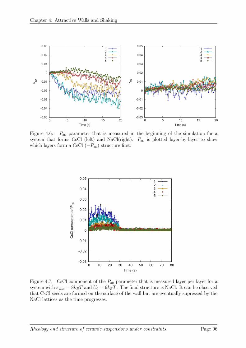
Chapter 4: Attractive Walls and Shaking
-0.05
-0.04
-0.03
-0.02
-0.01
0
0.01
0.02
0.03
0 5 10 15 20
P3D
Time (s)
12345
-0.03
-0.02
-0.01
0
0.01
0.02
0.03
0.04
0.05
0 5 10 15 20
P3D
Time (s)
12345
Figure 4.6: P3D parameter that is measured in the beginning of the simulation for asystem that forms CsCl (left) and NaCl(right). P3D is plotted layer-by-layer to showwhich layers form a CsCl (−P3D) structure first.
-0.03
-0.02
-0.01
0
0.01
0.02
0.03
0.04
0.05
0 10 20 30 40 50 60 70 80
CsC
l com
pone
nt o
f P3D
Time (s)
12345
Figure 4.7: CsCl component of the P3D parameter that is measured layer per layer for asystem with εWall = 8kBT and U0 = 9kBT . The final structure is NaCl. It can be observedthat CsCl seeds are formed on the surface of the wall but are eventually supressed by theNaCl lattices as the time progresses.
Rheology and structure of ceramic suspensions under constraints Page 96
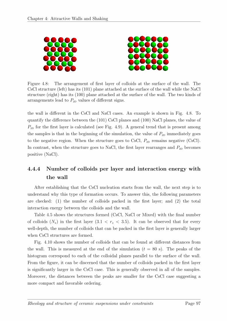
Chapter 4: Attractive Walls and Shaking
Figure 4.8: The arrangement of first layer of colloids at the surface of the wall. TheCsCl structure (left) has its (101) plane attached at the surface of the wall while the NaClstructure (right) has its (100) plane attached at the surface of the wall. The two kinds ofarrangements lead to P2D values of different signs.
the wall is different in the CsCl and NaCl cases. An example is shown in Fig. 4.8. To
quantify the difference between the (101) CsCl planes and (100) NaCl planes, the value of
P2D for the first layer is calculated (see Fig. 4.9). A general trend that is present among
the samples is that in the beginning of the simulation, the value of P2D immediately goes
to the negative region. When the structure goes to CsCl, P2D remains negative (CsCl).
In contrast, when the structure goes to NaCl, the first layer rearranges and P2D becomes
positive (NaCl).
4.4.4 Number of colloids per layer and interaction energy with
the wall
After establishing that the CsCl nucleation starts from the wall, the next step is to
understand why this type of formation occurs. To answer this, the following parameters
are checked: (1) the number of colloids packed in the first layer; and (2) the total
interaction energy between the colloids and the wall.
Table 4.5 shows the structures formed (CsCl, NaCl or Mixed) with the final number
of colloids (Ns) in the first layer (3.1 < rz < 3.5). It can be observed that for every
well-depth, the number of colloids that can be packed in the first layer is generally larger
when CsCl structures are formed.
Fig. 4.10 shows the number of colloids that can be found at different distances from
the wall. This is measured at the end of the simulation (t = 80 s). The peaks of the
histogram correspond to each of the colloidal planes parallel to the surface of the wall.
From the figure, it can be discerned that the number of colloids packed in the first layer
is significantly larger in the CsCl case. This is generally observed in all of the samples.
Moreover, the distances between the peaks are smaller for the CsCl case suggesting a
more compact and favorable ordering.
Rheology and structure of ceramic suspensions under constraints Page 97

Chapter 4: Attractive Walls and Shaking
-0.003
-0.002
-0.001
0
0.001
0.002
0.003
0 10 20 30 40 50 60 70 80
P2D
Time (s)
9kBT15kBT
Figure 4.9: P2D parameter for the system with κa = 1.5.
Table 4.5: Final number of colloids in the first layer with the corresponding structure.
κa = 1.5 Sample 1 Sample 2 Sample 3 Sample 4 Sample 57kBT 101 (CsCl) 89 (CsCl) 87 (CsCl) 89 (CsCl) 88 (CsCl)8kBT 81 (NaCl) 94 (CsCl) 88 (NaCl) 87 (NaCl) 96 (CsCl)9kBT 91 (NaCl) 94 (CsCl) 80 (Mixed) 76 (Mixed) 97 (CsCl)10kBT 90 (CsCl) 91 (CsCl) 91 (CsCl) 104 (CsCl) 99 (CsCl)κa = 2.55 Sample 1 Sample 2 Sample 3 Sample 4 Sample 57kBT 93 (NaCl) 74 (NaCl) 76 (Mixed) 56 (Mixed) 76 (NaCl)8kBT 86 (NaCl) 76 (Mixed) 77 (Mixed) 73 (Mixed) 73 (Mixed)9kBT 95 (NaCl) 75 (Mixed) 87 (NaCl) 82 (Mixed) 82 (CsCl)10kBT 79 (Mixed) 96 (NaCl) 105 (CsCl) 84 (Mixed) 86 (Mixed)
Rheology and structure of ceramic suspensions under constraints Page 98
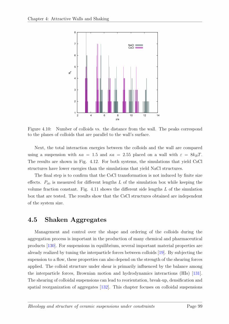
Chapter 4: Attractive Walls and Shaking
1
2
3
4
5
6
7
8
2 4 6 8 10 12 14
Ns
z/a
NaClCsCl
Figure 4.10: Number of colloids vs. the distance from the wall. The peaks correspondto the planes of colloids that are parallel to the wall’s surface.
Next, the total interaction energies between the colloids and the wall are compared
using a suspension with κa = 1.5 and κa = 2.55 placed on a wall with ε = 8kBT .
The results are shown in Fig. 4.12. For both systems, the simulations that yield CsCl
structures have lower energies than the simulations that yield NaCl structures.
The final step is to confirm that the CsCl transformation is not induced by finite size
effects. P3D is measured for different lengths L of the simulation box while keeping the
volume fraction constant. Fig. 4.11 shows the different side lengths L of the simulation
box that are tested. The results show that the CsCl structures obtained are independent
of the system size.
4.5 Shaken Aggregates
Management and control over the shape and ordering of the colloids during the
aggregation process is important in the production of many chemical and pharmaceutical
products [130]. For suspensions in equilibrium, several important material properties are
already realized by tuning the interparticle forces between colloids [19]. By subjecting the
supension to a flow, these properties can also depend on the strength of the shearing forces
applied. The colloid structure under shear is primarily influenced by the balance among
the interparticle forces, Brownian motion and hydrodynamics interactions (HIs) [131].
The shearing of colloidal suspensions can lead to reorientation, break-up, densification and
spatial reorganization of aggregates [132]. This chapter focuses on colloidal suspensions
Rheology and structure of ceramic suspensions under constraints Page 99

Chapter4:Attractive WallsandShaking
-0.3
-0.25
-0.2
-0.15
-0.1
-0.05
0
0.05
0 10 20 30 40 50 60 70 80
P3D
Time (s)
22a22.5a22.75a23a26a
Figure4.11: TheinfluenceofLontheparameterP3D
-2600
-2400
-2200
-2000
-1800
-1600
0 10 20 30 40 50 60 70 80
Energy (J)
Time (s)
NaCl (κ a = 1.5)CsCl (κ a = 1.5)NaCl (κ a = 2.55)CsCl (κ a = 2.55)
. TheresultsprovethattheformationofCsClstructuresisnotinducedbyfinitesizeeffects.
Figure4.12: Comparingthecolloid-wallinteractionenergiesforNaClvs.CsClstructures.Thestrengthofthewallusedin8kBTforbothκa=1.5and2.55interactionranges.
Rheologyandstructureofceramicsuspensionsunderconstraints Page100

Chapter 4: Attractive Walls and Shaking
subjected to oscillating flow.
In the work by Penkova et al., it was experimentally observed that shear flow may
strongly affect the nucleation in suspensions [120]. Morever in some systems, there is an
optimal flow velocity that can lead to the fastest nucleation [120, 133]. This rationale is
backed-up by Refs. [132, 134] where it was found that a small amount of shear can speed
up the crystallization process of colloids and enhances the quality of the growing crystal.
They also found that moderate shear rates can prevent or destroy ordering in the sytem.
However, the numerical studies mentioned above do not include a full treatment of
HIs. This can be problematic since the modeling of sheared suspensions without proper
HIs inclusion are known to induce colloid ordering [135]. The objective of this chapter
is to model aggregates under oscillatory flows using SRD-MD. Moreover, it attempts to
understand how the microstructure accomodates the applied shearing forces. The results
should provide qualitative insights onto the effects of shear and HIs on the crystallization
process of colloidal suspensions.
4.6 System: Modeling oscillatory flows
In Sec. 1.5.1, the way in which shear is introduced in the colloidal system is discussed.
Oscillatory motion is simulated by using the following line in the LEBC:
dvy = DELVY * cos ( 2 * pi * totaltime * FREQ )
The factor dvy is the shear velocity, DELVY describes the amplitude of oscillation,
while FREQ dictates the oscillation frequency of the system. The thermostat applied is
the Monte-Carlo thermostat discussed in Sec. 1.5.2.2.
The system used is the same the system described in Chapter 3 to facilitate
comparisons between the systems when the oscillating shear is removed. The colloids
have a radius of a = 255 nm and mass of 2.76 × 10⁻¹⁶. They are evolved using a DLVO
potential with the secondary minimum having a well-depth of 10kBT . Nc = 500 colloids
are placed in a simulation box of side length L = 55a0, where a0 = 127.5. The resulting
volume fraction is 10%.
The shear rate is set to 10 s−1 and the frequency of oscillations used is 20 s−1.
The equilibration is the part where the system, starting from a Maxwell-Boltzmann
distribution, starts receiving shearing forces until it reaches a steady state. Finding the
appropriate thermostat strength c for oscillatory flow proves to be more challenging and
time consuming than the one-directional flow presented in Chapter 2. It was found that
the equilibration part requires a stronger thermostat strength. However it also stabilizes to
a temperature lower than the required temperature (T < 293 K). Hence for the preliminary
investigations made in this chapter, the value of c used during the equilibration part is
Rheology and structure of ceramic suspensions under constraints Page 101

Chapter 4: Attractive Walls and Shaking
0
0.2
0.4
0.6
0.8
1
1.2
0 0.5 1 1.5 2 2.5 3
% o
f col
loid
s w
ith 1
2 ne
ares
t nei
ghbo
rs
Time (s)
c = 0.02 w/ shaking c = 0.01 w/ shakingc = 0.005 w/ shakingw/o shaking
Figure 4.13: Percentage of colloids with 12 nearest neighbors vs. time. The ordering ofthe shaken aggregates is generally larger than the ordering of the aggregates in equilibrium.
c = 0.02. Values of c < 0.02 are too small for the equilibration procedure and lead to
anomalous behavior. Once the temperature T stabilizes, the value of c is varied. In this
work, c = 0.02, 0.01 and 0.005 are used.
4.7 Results for Shaken Aggregates
First, the SRD-MD simulations of shaken aggregates are compared with the SRD
simulations in equilibrium. The results are shown in Fig. 4.14. Despite the different
temperatures in the three systems, a general trend can be observed. That is, the ordering
for the shaken aggregates is larger and faster than the ordering of the aggregates in
equilibrium.
Second, the SRD-MD simulations of shaken aggregates with c = 0.02 are compared
with SRD-MD and BD simulations of aggregates in equilibrium. The results are shown
in Fig. 4.13. The shaken aggregates are more ordered than its SRD-MD equilibrium
counterpart while also achieving the same ordering as the BD simulations. Overall, the
oscillatory flow promotes faster ordering within the aggregate.
The aggregate formation are also checked by plotting NA vs time. This is shown in
Fig. 4.15. It seems that when the aggregates undergo an oscillating shear, the cluster-
cluster coalescence is slower. If we follow the same logic as in Chapter 3, i.e. the slow
cluster-cluster coalescence promotes ordering within the aggregate, then the shaking may
provide the colloids enough time to reorganize within the small clusters.
Rheology and structure of ceramic suspensions under constraints Page 102

Chapter 4: Attractive Walls and Shaking
0
0.2
0.4
0.6
0.8
1
1.2
0 0.5 1 1.5 2 2.5 3
% o
f col
loid
s w
ith 1
2 ne
ares
t nei
ghbo
rs
Time (s)
SRD w/ shakingSRD w/o shakingBD w/o shaking
Figure 4.14: Percentage of colloids with 12 nearest neighbors vs. time for SRD and BDsimulations.
1
10
100
1000
0.01 0.1 1
NA
Time (s)
SRD w/ shakingSRD w/o shakingBD w/o shaking
Figure 4.15: Number of Aggregates (NA) vs time for systems with and without shaking.
Rheology and structure of ceramic suspensions under constraints Page 103

Chapter 4: Attractive Walls and Shaking
4.8 Conclusions
First, this chapter has demonstrated that by using Brownian Dynamics simulations
and by introducing an attractive wall to a binary system of colloids, the expected
equilibrium lattice structure can be reordered. The extent of lattice transformation
depends on the properties of the suspension and the characteristics of the walls.
Specifically, when the strength of attraction of the wall supersedes the strength of
attraction between the colloids (εWall > U0), the probability of forming a CsCl structure is
higher than its metastable NaCl-counterpart. However, when εWall < U0, most aggragates
are formed with NaCl structures as in the absence of the wall.
Additionally, the suspensions with κa = 1.5 are more susceptible to change than
suspensions with κa = 2.55 and κa = 3. This is because aggregation is more difficult
for κa = 1.5 thus making it more adaptable to the phase transformation caused by the
attractive wall.
It was also observed that CsCl-seeds start forming at the bottom of the wall and slowly
build up to the top most layers. CsCl formation is more favorable because it allows the
colloids to be more closely packed at the surface. In addition to this, it was observed that
the interaction energy, between the colloids and the walls, is also lower for CsCl structures
than for NaCl structures.
From the results presented, it appears that the process of undergoing metastable NaCl
formation can be skipped when a sufficiently strong wall is introduced to the original
system. Moreover, for κa < 2.55, CsCl structures would be metastable in absence of the
wall.
However, it is important to note that hydrodynamic effects are ignored in this chapter
for the following reasons: (1) the study serves as a preliminary analysis on the effects of
attractive walls on colloids, (2) the suspensions are still relatively dilute, (3) HIs are found
to be negligible in the aggregation of the bulk system presented in Ref. [39]. Nevertheless,
the incorporation of HIs can serve as a possible extension on the study of colloid adsorption
on surfaces.
Finally, this chapter also provides preliminary investigations concerning aggregates
under oscillatory flow. It was found that in general, when aggregates are subjected to an
oscillating shear, the ordering of the colloids increases. In addition to this, the rate of
ordering is faster. While several tests and samplings have to be performed, we argue that
the results provided can give a good qualitative insight into the effects of oscillatory flows
in shaken aggregates, especially since the system requires proper HIs modeling.
A better thermostat that fits the shaken aggregates is also needed. While the Monte-
Carlo thermostat can still be applied in the system presented in this chapter, finding the
required c value proves to be time and memory consuming. A good extension of this work
Rheology and structure of ceramic suspensions under constraints Page 104

Chapter 4: Attractive Walls and Shaking
is to generate an SRD-MD-appropriate thermostat that can accomodate different shear
forces.
Rheology and structure of ceramic suspensions under constraints Page 105

Conclusions
Conclusions
Rheology and structure of ceramic suspensions under constraints Page 106

Conclusions
In this thesis, two of the main challenges in the computational study of colloidal
suspensions are addressed: incorporation of hydrodynamic interactions (HIs) and the
modeling of external constraints in the forms of shear and attractive wall.
First, the hybrid Stochastic Rotation Dynamics - Molecular Dynamics (SRD-MD)
method was developed. In contrast to previous works, the method presented in this
thesis was able to calculate for the shear viscosity vs. volume fraction relation of a system
that resembles a hard-sphere interaction. This was achieved by implementing the Lees-
Edwards boundary conditions (LEBC) for a system with an MD-type coupling. Since the
addition of shear generates energy drifts, a Monte-Carlo thermostat was also employed.
The steady state condition generated by the LEBC and Monte-Carlo algorithms was
described by stress tensors, from which the shear viscosity was evaluated. The presented
non-equilibrium approach of obtaining the shear viscosity can be applied to both dense and
concentrated cases. Moreover, it can be used to analyze the components of shear viscosity
and the characterization can be done in two ways: one is by examining the kinetic and
collision contributions, and the other is by examining the fluid and colloid contributions.
The SRD-MD results are also comparable with known numerical, experimental and
theoretical data
At this stage, SRD-MD has been verified and can be used alongside Brownian
Dynamics (BD) to determine the percolation threshold (φc) of alumina suspensions
described by the Derjaguin-Landau-Verwey-Overbeek potential. The BD simulations
successfully provided a phase-space diagram (volume fraction vs. colloid-colloid attraction
strength) that gives an approximation of the region where percolation in 3 directions can
be observed. Moreover, the phase-space diagram shows that φc decreases with increasing
colloid-colloid attraction strength. Additional information regarding the effects of HIs on
φc were found using SRD-MD. Specifically, systems with HIs tend to have more elongated
structures during the aggregation process than systems without HIs. There is a significant
decrease in φc when the colloid-colloid attraction is not too strong (for a well depth of
5kBT , φc = 10% with HIs and φc = 12% without HIs). On the other hand, the effects
of HIs tend to become negligible when the colloid-colloid attraction increases (for a well
depth of 10kBT , φc = 8% with or without HIs). These observations have also huge
implications in solving the problem of long computation times that are often required
in modeling percolating systems. A good indicator for determining the most appropriate
simulation technique is the colloid-colloid attraction strength. For systems with attraction
strengths greater than 10kBT , the rearrangement process is very slow hence BD should
suffice. In contrast, for systems with attraction strengths less than 10kBT , SRD-MD is
among the fastest approach available that can properly account for HIs. The φc values
calculated in this thesis are in also in good agreement with those estimated by the yield
stress model (YODEL) by Flatt and Bowen. This work can be useful, alongside YODEL,
Rheology and structure of ceramic suspensions under constraints Page 107

Conclusions
in predicting the yield stress magnitude of ceramic materials.
Another type of external force introduced in this thesis is in the form of an attractive
wall. A binary system of colloids described by the Yukawa potential was placed in a
simulation box with one attractive surface and is modeled using BD. The behaviour of the
binary system in equilibrium is already known from previous studies: for suspensions with
a well depth of 9kBT , NaCl-type lattices are energetically stable when κa < 2.55, where
κa describes the inverse range of interaction; and CsCl-type lattices are energetically
stable when κa > 2.55. This behaviour is altered with the introduction of the wall.
It was established that when the wall’s attraction strength surpasses the colloid-colloid
attraction strength, the NaCl lattices tend to transform to CsCl. The probability of
this lattice modification is even higher as the attraction strength of the wall increases.
Aside from the wall’s attraction strength, the effect of changing the value of κa was also
investigated. The results show that smaller values of κa, e.g. κa = 1.5 and 1, are more
susceptible to lattice changes than higher values of κa, e.g. κa = 3 and 2.55. This is
because aggregation is more difficult to achieve for κa ≤ 1.5. By looking at the final
structures, it can be seen that the CsCl lattice formation is more favored when the wall
is sufficiently strong because it allows for a more compact configuration. In addition to
this, it was found that the total energy between the wall and the structure is also lower
for the CsCl case than the NaCl case.
Finally, preliminary investigations on shaken suspensions by SRD-MD were conducted.
The 10kBT -case alumina system, which does not attain proper reorganization, was
placed under an oscillating shear with a rate of 10 s−1 and a frequency of 20 s−1.
This is to check if the ordering of the structure improves. The results show that the
suspensions undergoing oscillatory motion reorganize at a faster rate than the suspensions
in equilibrium. This technique of agitating the suspension can have a high potential in
promoting crystallization and requires a more in-depth study.
Rheology and structure of ceramic suspensions under constraints Page 108

Bibliography
Bibliography
Rheology and structure of ceramic suspensions under constraints Page 109

Bibliography
[1] T. Ihle and D. M. Kroll, Phys. Rev. E., vol. 67, p. 066705, 2003.
[2] N. Kikuchi, M. Pooley, J. F. Ryder, and J. M. Yeomans, J. Chem. Phys., vol. 119,
p. 6388, 2003.
[3] D. R. Foss and J. F. Brady, J. Rheology, vol. 44, p. 629, 2000.
[4] J. M. Koelman and P. J. Hoogerbrugge, Europhys. Lett., vol. 21, pp. 363–368, 1993.
[5] P. J. Hoogerbrugge and J. M. V. A. Koelman, Europhys. Lett., vol. 19, pp. 155–160,
1992.
[6] P. N. Segre, S. P. Meeker, P. N. Pusey, and W. C. K. Poon, Phys. Rev. Lett., vol. 75,
no. 5, p. 958, 1995.
[7] J. van der Werff and C. de Kruif, J. Rheology, vol. 33, p. 421, 1989.
[8] I. M. Krieger and T. J. Dougherty, Trans. Soc. Rheol. III, vol. 1959, p. 137, 1959.
[9] A. Einstein, Ann. Phys., vol. 19, p. 289, 1906.
[10] ——, Ann. Phys., vol. 34, p. 591, 1911.
[11] O. O. Omatete, M. A. Janney, and R. A. Strehlow, Am. Ceram. Soc. Bull., vol. 70,
pp. 1641–1649, 1991.
[12] M. Agarwala, A. Bandyopadhyay, and R. van Weerwn, Am. Ceram. Soc. Bull.,
vol. 75, pp. 60–66, 1996.
[13] J. Cesarano, R. Segalman, and P. Calvert, Ceram. Ind., pp. 94–102, 1998.
[14] M. L. Griffith and J. W. Halloran, J. Am. Ceram. Soc, vol. 79, pp. 2601–2608, 1996.
[15] E. Sachs, M. Cima, and P. Williams, J. Eng. Ind., vol. 114, pp. 481–488, 1992.
[16] M. E. Leunissen, C. Christova, A. P. Hynninen, C. P. Royall, A. I. Campbell,
A. Imhof, M. Dijkstra, R. van Roij, and A. van Blaaderen, Nature, vol. 437, p. 235,
2005.
[17] B. V. Derjaguin and L. D. Landau, Acta Physicochim. URSS, vol. 14, p. 63352,
1941.
[18] E. . J. W. Verwey and J. T. G. Overbeek, Theory of Stability of Lyophobic Colloids.
The Netherlands: Elsevier, 1948.
[19] J. A. Lewis, J. Am. Ceram. Soc., vol. 83, pp. 2341–59, 2000.
Rheology and structure of ceramic suspensions under constraints Page 110
Bibliography
[20] C. N. Likos, Physics Reports, vol. 348, pp. 267–439, 2001.
[21] M. Stuer and P. Bowen, Adv. Appl. Ceramics, vol. 11, pp. 254–261, 2012.
[22] R. Flatt and P. Bowen, J. Am. Cream. Soc., vol. 89, pp. 1244–1256, 2006.
[23] P. Lu, E. Zaccarelli, F. Ciulla, A. Schofield, F. Sciortino, and D. A. Weitz, Nature,
vol. 453, pp. 499–503, 2008.
[24] B. D’unweg and A. J. C. Ladd, Advance computer simulation approaches for soft
matter sciences III, 1st ed. Berlin: Springer, 2009, vol. 3, ch. 2, pp. 90–166.
[25] A. Malevanets and R. Kapral, J. Chem. Phys., vol. 1999, p. 8605, 110.
[26] M. Stuer, Z. Zhao, U. Aschauer, and P. Bowen, J. Eur. Ceram. Soc., vol. 30, pp.
1335–1343, 2010.
[27] M. P. Allen and D. J. Tildesley, Classical Mechanics 2nd ed. Oxford UK: Addison
Wesley, 1980.
[28] Y. Li, Y. Huo, and Y. Zhang, Colloid Polym. Sci., pp. 1–9, 2015.
[29] G. Gompper, T. Ihle, D. M. Kroll, and R. G. Winkler, Advance computer simulation
approaches for soft matter sciences III, 1st ed. Berlin: Springer, 2009, vol. 3, ch. 1,
pp. 1–88.
[30] J. T. Padding and A. A. Louis, Phys. Rev. E., vol. 74, p. 031402, 2006.
[31] M. Hecht, J. Harting, M. Bier, J. Reinshagen, and H. Herrmann, Phys. Rev. E.,
vol. 74, p. 021403, 2006.
[32] C. Holm and K. Kremer, Eds., Advance computer simulation approaches for soft
matter sciences III, 1st ed. Berlin: Springer, 2009, vol. 3.
[33] B. J. Alder and T. E. Wainwright, J. Chem. Phys., vol. 31, p. 459, 1959.
[34] ——, J. Chem. Phys., vol. 33, p. 1439, 1960.
[35] B. J. Alder, D. M. Gass, and T. E. Wainwright, J. Chem. Phys., vol. 53, p. 3813,
1970.
[36] D. L. Ermak and A. J. McCammon, J. Chem. Phys., vol. 69, pp. 1352–1360, 1978.
[37] M. Cerbelaud, A. Videcoq, P. Abelard, C. Pagnoux, F. Rossignol, and R. Ferrando,
Langmuir, vol. 24, pp. 3001–3008, 2008.
Rheology and structure of ceramic suspensions under constraints Page 111

Bibliography
[38] M. A. Piechowiak, A. Videcoq, R. Ferrando, D. Bochicchio, C. Pagnoux, and
F. Rossignol, Phys. Chem. Chem. Phys., vol. 14, pp. 1431–1439, 2012.
[39] D. Bochicchio, A. Videcoq, and R. Ferrrando, Phys. Rev. E., vol. 87, p. 022304,
2013.
[40] J. Rotne and S. Prager, J. Chem. Phys., vol. 50, p. 4831, 1969.
[41] H. Yamakawa, J. Chem. Phys., vol. 53, pp. 436–443, 1970.
[42] V. Pryamitsyn and V. Ganesan, J. Chem. Phys., vol. 122, p. 104906, 2005.
[43] P. Espanol and P. Warren, Euro. Phys. Lett., vol. 30, pp. 191–196, 1995.
[44] J. E. Broadwell, J. Fluid Mech., vol. 19, pp. 401–414, 1964.
[45] S. Chen and G. D. Doolen, Annu. Rev. Fluid Mech., vol. 30, pp. 329–364, 1998.
[46] S. Ollila, C. Denniston, M. Karttunen, and T. Ala-Nissila, J. Chem. Phys., vol. 134,
p. 064902, 2011.
[47] A. J. C. Ladd, J. Fluid Mech, vol. 271, p. 285, 1994.
[48] A. Malevanets and R. Kapral, J. Chem. Phys., vol. 112, p. 7260, 2000.
[49] R. Kapral, Adv. Chem. Phys., vol. 140, p. 89, 2008.
[50] R. G. Winkler and C. C. Huang, J. Chem. Phys., vol. 130, p. 074907, 2009.
[51] H. Goldstein, C. Poole, and J. Safko, Classical Mechanics. Oxford UK: Oxford
University Press, 1987.
[52] C. C. Huang, A. Chatterji, G. Sutmann, G. Gompper, and R. G. Winkler, J. Comp.
Phys., vol. 229, pp. 168–177, 2010.
[53] A. Nikoubashman, N. A. Mahynski, A. H. Pirayandeh, and A. Z. Panagiotopoulos,
J. Chem. Phys., vol. 140, p. 094903, 2014.
[54] H. Lowen, Phys. Rev. E., vol. 53, p. R29, 1996.
[55] E. Allahyarov and G. Gommper, Phys. Rev. E., vol. 66, p. 036702, 2002.
[56] A. Lamura, G. Gommper, T. Ihle, and D. M. Kroll, Europhys. Lett., vol. 73, p. 664,
2001.
[57] J. K. Whitmer and E. Luijten, J. Phys.: Condens. Matt., vol. 22, p. 104106, 2010.
Rheology and structure of ceramic suspensions under constraints Page 112

Bibliography
[58] A. W. Lees and S. F. Edwards, J. Phys. C: Solid State Phys., vol. 5, pp. 1921–1929,
1972.
[59] P. H. Hunenberger, Adv. Polym. Sci., vol. 173, pp. 105–149, 2005.
[60] H. C. Andersen, J. Chem. Phys., vol. 72, pp. 2384–2393, 1980.
[61] S. Nose, J. Chem. Phys., vol. 81, p. 511, 1984.
[62] W. G. Hoover, D. J. Evans, R. B. Hickman, A. J. C. Ladd, W. T. Ashurst, and
B. Moran, Physical Review A, vol. 22, pp. 1690–1697, 1980.
[63] A. Tomilov, A. Videcoq, T. Chartier, T. Ala-Nissila, and I. Vattulainen, J. Chem.
Phys., vol. 137, p. 014503, 2012.
[64] D. M. Heyes, Chem. Phys., vol. 82, pp. 285–301, 1983.
[65] M. Hecht, J. Harting, T. Ihle, and H. Herrmann, Phys. Rev. E., vol. 72, p. 011408,
2005.
[66] H. Noguchi and G. Gompper, Phys. Rev. E, vol. 78, p. 016706, 2008.
[67] C. M. Pooley and J. M. Yeomans, J. Phys. Chem. B, vol. 109, p. 65015, 2005.
[68] G. Batot, V. Dahirel, G. Meriguet, A. Louis, and M. Jardat, Phys. Rev. E., vol. 88,
p. 043304, 2013.
[69] J. K. Whitmer and E. Luijten, J. Phys.: Condens. Matter, vol. 22, p. 104106, 2010.
[70] A. A. Louis, E. Allahyarov, H. Lowen, and R. Roth, Phys. Rev. E., vol. 65, p.
061407, 2002.
[71] J. M. Brader, J. Phys., vol. 22, p. 363101, 2010.
[72] D. B. Genovese, Advances in Colloid and Interface Science, vol. 171-172, pp. 1–16,
2012.
[73] R. A. Lionberger and W. B. Russel, J. Chem. Phys., vol. 106, p. 402, 1997.
[74] G. K. Batchelor and J. Green, J. Fluid Mech., vol. 56, p. 401, 1972.
[75] A. Tomilov, A. Videcoq, M. Cerbelaud, M. A. Piechowiak, T. Chartier, T. Ala-
Nissila, D. Bochicchio, and R. Ferrando, J. Phys. Chem. B, vol. 117, p. 14509,
2013.
[76] M. S. Green, J. Chem. Phys., vol. 22, p. 398, 1954.
Rheology and structure of ceramic suspensions under constraints Page 113

Bibliography
[77] R. Kubo, J. Phys. Soc. Japan, vol. 12, pp. 570–586, 1957.
[78] H. Mori, Prog. Theor. Phys., vol. 33, p. 423, 1965.
[79] ——, Prog. Theor. Phys., vol. 34, p. 399, 1965.
[80] R. Zwanzig, Lectures in Theoretical Physics. New York: Wiley, 1961, vol. 3.
[81] S. Mueller, E. W. Llewellin, and H. M. Mader, Proc. R. Soc. A., vol. 466, pp.
1201–1228, 2010.
[82] D. G. Thomas, J. Colloid Sci., vol. 20, pp. 267–277, 1965.
[83] I. R. Rutgers, Rheol. Acta, vol. 2, pp. 202–210, 1962.
[84] ——, Rheol. Acta, vol. 2, pp. 305–348, 1962.
[85] E. Guth and O. Gold, Phys. Rev., vol. 53, p. 322, 1938.
[86] V. Vand, J. Phys. Colloid Chem., vol. 52, pp. 277–299, 1948.
[87] R. S. J. Manley and S. G. Mason, Can J. Chem., vol. 33, pp. 733–763, 1955.
[88] J. T. Padding and A. A. Louis, Phys. Rev. Lett., vol. 93, p. 220601, 2004.
[89] W. K. Poon, E. R. Weeks, and C. P. Royall, Soft Matter, vol. 8, pp. 21–30, 2012.
[90] A. Laganapan, A. Videcoq, M. Bienia, T. Ala-Nissila, D. Bochicchio, and
R. Ferrando, J. Chem. Phys., vol. 142, p. 144101, 2015.
[91] D. M. Heyes and J. R. Melrose, J. Non-Newtonian Fluid Mech., vol. 46, pp. 1–28,
1993.
[92] J. F. Brady and J. F. Morris, J. Fluid Mech., vol. 348, pp. 103–139, 1997.
[93] D. Quemada and C. Berli, Adv. Colloid and Interface Sci., vol. 98, pp. 51–85, 2002.
[94] F. Y. Castillo, R. Socher, B. Krause, R. Headrick, B. P. Grady, R. Prada-Silvy, and
P. Potschke, Polymer, vol. 52, pp. 3835–3845, 2011.
[95] A. Coniglio, L. D. Arcangelis, E. D. Gado, A. Fierro, and N. Sator, J. Phys.:
Condens. Matt., vol. 16, pp. 4831–4839, 2004.
[96] M. E. Helgeson, Y. Gao, S. E. Moran, J. Lee, M. Godfrin, A. Tripathi, A. Bose,
and P. S. Doyle, Soft Matter, vol. 17, pp. 3122–33, 2014.
[97] J. Bergenholtz and M. Fuchs, Phys. Rev. E., vol. 59, pp. 5706–5715, 1999.
Rheology and structure of ceramic suspensions under constraints Page 114

Bibliography
[98] A. Coniglio, J. J. Arenzon, A. Fierro, and M. Sellito, Eur. Phys. J. Special Topics,
vol. 223, pp. 2297–2306, 2014.
[99] S. R. Broadbent and J. M. Hammersley, Proc. Camb. Philos. Soc., vol. 53, pp.
629–641, 1957.
[100] Z. Zhou, M. J. Solomon, P. J. Scales, and D. V. Boger, J. Rheology, vol. 43, pp.
651–671, 1999.
[101] I. Lesov, S. Tcholakova, and N. Denkov, J. Colloid and Interface Science, vol. 426,
pp. 9–21, 2014.
[102] R. M. Guillermic, A. Salonen, J. Emile, and A. Saint-Jalmes, Soft Matter, vol. 5,
pp. 4975–4982, 2009.
[103] M. Strauss, T. Ring, A. Bleier, and H. K. Bowen, J. App. Phys., vol. 58, p. 3871,
1985.
[104] P. C. Kapur, P. J. Scales, D. V. Boger, and T. W. Healy, AIChe. J., vol. 43, pp.
1171–1179, 1997.
[105] P. J. Scales, T. W. H. S. B. Johnson, and P. C. Kapur, AIChe. J., vol. 44, pp.
538–544, 1998.
[106] A. Moncho-Jorda, A. A. Louis, and J. T. Padding, Phys. Rev. Lett., vol. 104, p.
068301, 2010.
[107] H. Tanaka and T. Araki, Phys. Rev. Lett., vol. 85, pp. 1338–1341, 2000.
[108] I. M. Janosi, T. Tel, D. E. Wolf, and J. A. C. Gallas, Phys. Rev. E., vol. 56, pp.
2858–2867, 1997.
[109] R. Yamamoto, K. Kim, Y. Nakayama, K. Miyazaki, and D. Reichman, J. Phys. Soc.
Japan, vol. 77, p. 084804, 2008.
[110] J. Whitmer and E. Luijten, J. Phys. Chem. B, vol. 115, pp. 7294–7300, 2011.
[111] A. Laganapan, M. Mouas, A. Videcoq, M. Cerbelaud, M. Bienia, P. Bowen, and
R. Ferrando, J. Colloids and Interface Science, vol. 458, pp. 241–246, 2015.
[112] L. Bergstrom, Adv. Colloid Interface Sci, vol. 70, p. 125, 1997.
[113] D. Bochicchio, A. Videcoq, A. R. Studart, and R. Ferrrando, J. Colloid Interface
Sci., vol. 440, pp. 198–203, 2015.
Rheology and structure of ceramic suspensions under constraints Page 115

Bibliography
[114] M. Cerbelaud, R. Ferrando, and A. Videcoq, J. Chem. Phys., vol. 132, p. 084701,
2010.
[115] A. Larsen and D. Grier, Nature, vol. 385, pp. 230–233, 1997.
[116] M. Buerger, Phase Transformations in Solids. New York: Wiley, 1951.
[117] D. Zahn, O. Hochrein, and S. Leoni, Phys. Rev. B, vol. 72, p. 094106, 2005.
[118] P. Gonzales-Mozuelos, M. Medina-Noyola, B. D’Aguanno, J. M. Mendez-Alcaraz,
and R. Klein, J. Chem. Phys., vol. 95, p. 3, 1991.
[119] M. Oberholzer, N. J. Wagner, and A. M. Lenhoff, J. Chem. Phys., vol. 107, p. 9157,
1997.
[120] A. Penkova, W. Pan, F. Hodjaoglu, and P. G. Vekilov, Ann. N. Y. Acad. Sci., vol.
214, p. 1077, 2006.
[121] A. Yethiraj and A. A. van Blaaderen, Nature, vol. 421, pp. 513–517, 2003.
[122] W. K. Kegel and A. van Blaaderen, Science, vol. 287, pp. 290–293, 2000.
[123] M. Malmsten, J. Colloid and Interface Sci., vol. 207, pp. 186–199, 1998.
[124] C. A. Haynes and W. Norde, Colloids Surf., vol. 2, p. 517, 1994.
[125] Y. F. Missirlis and W. Lemm, Modern Aspects of Protein Adsorption on
Biomaterials. Boston: Kluwer Academic, 1991.
[126] K. P. Velikov, C. G. Christova, R. P. A. Dullens, and A. van Blaanderen, Science,
vol. 296, pp. 106–109, 2002.
[127] E. C. M. Vermolen, A. Kuijk, L. C. Filion, M. Hermes, J. H. J. Thijssen, M. Dijkstra,
and A. van Blaaderen, Proc Natl Acad Sci U S A, vol. 106, pp. 16 063–16 067, 2009.
[128] D. Bochicchio, A. Videcoq, and R. Ferrrando, J. Chem. Phys., vol. 140, p. 024911,
2014.
[129] D. van der Spoel, E. Lindahl, B. Hess, G. Groenhof, A. E. Mark, and H. J. C.
Berendsen, J. Comput. Chem, vol. 26, p. 1701, 2005.
[130] D. Li and R. B. Kaner, J. Am. Chem. Soc., vol. 128, pp. 968–975, 2005.
[131] J. Vermant and M. J. Solomon, J. Phys.: Condens. Matter, vol. 17, pp. R187–R216,
2005.
Rheology and structure of ceramic suspensions under constraints Page 116

Bibliography
[132] J. J. Cerda, T. Cintes, C. Holm, C. M. Sorensen, and A. Chakrabali, Phys. Rev. E.,
vol. 78, p. 031403, 2008.
[133] P. Vekilov, B. R. Thomas, and F. Rosenberger, J. Phys. Chem., vol. 102, pp. 5208–
5216, 1998.
[134] A. Mokshin and J. L. Barrat, Phys. Rev. E., vol. 82, p. 021505, 2010.
[135] J. F. Brady, Chem. Eng. Sci., vol. 56, pp. 2921–2926, 2001.
Rheology and structure of ceramic suspensions under constraints Page 117