© 2020 SCTE•ISBE and NCTA. All rights reserved. 1

RF Testing Applications for Software-Defined Radio

Using SDR for Impairment Generation

A Technical Paper prepared for SCTE•ISBE by

Robert M. Lund Principal Engineer

Next Generation Access Networks Comcast

720-512-3691 Robert_Lund@comcast.com

Kathryn Sanders

Intern / UIUC Undergraduate Student Sanders RF Consulting LLC

Kgs5@illinois.edu

© 2020 SCTE•ISBE and NCTA. All rights reserved. 2

Table of Contents Title Page Number

1. Introduction .................................................................................................................................... 3 2. Software-Defined Radio General Architecture ................................................................................ 3 3. SDR Software: GNU Radio ............................................................................................................ 5 4. Sampling Theory ............................................................................................................................ 6 5. The Discrete Fourier Transform or DFT .......................................................................................... 8 6. Introduction to Profile Management Application ............................................................................ 10 7. Practical Application Example #1– Capturing LTE Signals For Replay as an Impairment Source

.................................................................................................................................................... 12 8. Practical Application Example #2 – How SDR Has Aided Profile Management Application (PMA)

Testing ......................................................................................................................................... 15 9. Equipment Used .......................................................................................................................... 22 10. Conclusion ................................................................................................................................... 23

Abbreviations......................................................................................................................................... 24

Bibliography & References .................................................................................................................... 25

List of Figures Title Page Number Figure 1 – SDR Architecture Block Diagram ............................................................................................. 4 Figure 2 - GNU Radio Flowgraph Example .............................................................................................. 6 Figure 3 – Aliasing Due to Undersampling ............................................................................................... 7 Figure 4 – Square Wave Construction From Sine Waves ......................................................................... 8 Figure 5 – The Profile Management Application System ........................................................................ 11 Figure 6 – PMA In Action: Building Custom OFDM Profiles .................................................................... 11 Figure 7 - Finding LTE Band In Use on iPhone ...................................................................................... 12 Figure 8 - Real Time Spectrum Analyzers for IQ Capture (clockwise): osmocom_fft, uhd_fft, gqrx SDR

...................................................................................................................................................... 14 Figure 9 - Combining of Noise Sources in Laboratory Environment ........................................................ 14 Figure 10 - GRC Flowgraph to Contruct and Transmit Custom Impairment Waveform ............................ 17 Figure 11 - Graph of RxMER Data Generated by Embedded Python Block ............................................ 18 Figure 12 - Qt GUI Frequency Sink Visualization of Impairment Signal ................................................... 19 Figure 13 - Qt Fosphor Sink Visualization of Impairment Signal ............................................................. 19 Figure 14 - Bandwith Monitor of IQ Data Stream .................................................................................... 20 Figure 15 - Impairment Signal on Spectrum Analyzer ............................................................................. 21 Figure 16 - OFDM Profile for SDR Generated Impairment Signal ........................................................... 21

List of Tables Title Page Number Table 1 – LTE Frequency Bands (3) ...................................................................................................... 13 Table 2 – RxMER TFTP File Format (4) ................................................................................................. 16

© 2020 SCTE•ISBE and NCTA. All rights reserved. 3

1. Introduction Recent advances in digital communications algorithms and artificial intelligence, coupled with the exponential growth of personal computing power, have positioned software-defined radio (SDR) technology as a viable tool for RF signal capture and playback, simulation, and testing. Popular applications for modern SDR designs include:

• Cellular handsets with programmable digital signal processing (DSP) • University research / teaching aids • Military and satellite communications platforms that make use of programmable cores for

intermediate frequency (IF) and baseband signal processing • Cognitive radio – a “smart” radio mesh that can adapt to interference adjusting frequency

or power for example • Amateur radio

The goal of this paper is to outline the general architecture and capabilities of a software-defined radio, followed by some basic principles of digital signal processing. A familiarity with sampling theory and the discrete Fourier transform, for example, will be very helpful for anyone looking to get started with SDR. Finally, two lab applications of software-defined radio will be detailed. Both of these applications were used in testing a profile management application implementation, so a section on PMA is introduced. After familiarization with PMA, the first test example uses SDR to capture long term evolution (LTE) signals, then re-play them back into the RF plant to be subsequently detected by pattern recognition software that is a function of PMA. The second case recreates plant conditions from a cable modem’s perspective by translating its reported receive modulation error ratio (RxMER) values into a waveform to be used as an impairment profile applied to an orthogonal frequency division multiplexing (OFDM) channel. Again, this impairment can then be analyzed by the analytics engine of PMA, and a custom OFDM profile recommendation can be verified. 2. Software-Defined Radio General Architecture A software-defined radio is a radio that replaces traditional hardware components such as mixers, filters, and modulator/demodulators with software implementations, typically running on personal computers and driving a minimalistic hardware set. The Wireless Innovation Forum and IEEE P1900.1 working group has further simplified the definition down to: "Radio in which some or all of the physical layer functions are software defined" (1) There are many advantages to software-defined radio designs. Potentially first among these is the low cost. Devices can range from $10 USB-powered dongles, up to $10,000 high performance units with multiple transmit/receive (TX/RX) channels, higher maximum sampling rates, and greater usable bandwidth. Another primary advantage is flexibility. SDRs are not hardware limited to any particular specification standard, modulation type, or operating frequency range,

© 2020 SCTE•ISBE and NCTA. All rights reserved. 4

for example. The ability to test new designs in software also aids in the rapid prototyping of communication systems. Conceptually, an ideal software-defined radio would eliminate any analog signal processing stages, aside from an antenna, power amplifier, and input/output (I/O) sink or source such as a speaker or microphone. In reality, today’s SDRs use an analog frequency conversion stage at the receiver, with all signal processing thereafter being digital. Similarly at the transmitter, the digital-to-analog conversion stage is followed by local oscillator/mixer for transmit frequency conversion along with power amplification. To illustrate a typical SDR design, the block diagram in Figure 1 outlines the functional components. This was the hardware used in the two practical example sections to follow.

Figure 1 – SDR Architecture Block Diagram

The key features of this design include:

• Xilinx Zynq-7100 FPGA SoC • Dual-core ARM A9 800 MHz CPU • Two RX, two TX in half-wide RU form factor • 3 MHz to 6 GHz frequency range • Up to 200 MHz of instantaneous bandwidth per channel • Sub-octave RX, TX filter bank • 14 bit ADC, 16 bit DAC • Configurable sample rates: 200, 245.76, 250 MS/s • Two SFP+ ports (1 GbE, 10 GbE, Aurora, White Rabbit) • One QSFP+ port ( 2x 10 Gb / Aurora ) • RJ45 (1 GbE) • 10 MHz clock reference • PPS time reference

© 2020 SCTE•ISBE and NCTA. All rights reserved. 5

• External RX, TX LO input ports • Built-in GPSDO

One of the main factors to consider in selecting a radio is usable bandwidth. The specification above lists 200 MHz of available bandwidth that will allow us to simulate or impair a full OFDM block with 190 MHz of modulated spectrum. Another point to consider is sampling rate. Radios range from fixed, to selectable, to fully configurable sampling rates, with the fully configurable ones being the most flexible, because in some cases they can eliminate the need for additional resampling functions. Many designs use open-source Verilog code for the FPGA that can be modified for high performance applications. 3. SDR Software: GNU Radio GNU Radio is a free open-source development project that implements signal processing blocks in software for waveform creation, sampling, and analysis, that supports a variety of software-defined radio hardware. It is used extensively in academic and commercial environments for wireless communications research and real-world radio systems. GNU Radio consists of software-based signal processing blocks used in conjunction with hardware drivers to build applications capable of transmitting or receiving digital data streams. These streams can be directed to disk and saved in different file formats, or to a software-defined radio sink. GNU Radio resource blocks include equalizers, filters, modulators/demodulators, filters, and other common radio elements. These blocks’ inputs and outputs are then connected in software to build an end-to-end flow. Being software based, GNU Radio operates on digital data. It uses complex baseband samples as input for receivers and as the output data type for transmitters. Analog mixing hardware can then shift the signal to the proper frequency. One of the biggest advantages to working with GNU Radio is that it is primarily written using the Python programming language, with the computationally intensive operations written in C++. GNU Radio also incorporates a graphical user interface – creatively named GNU Radio Companion – that offers drag-and-drop software blocks to construct flowgraph applications. These GRC flowgraphs present an intuitive approach to thinking about the discrete signal processing stages. Once a flowgraph contains a source and sink, the file can be saved and executed, and Python code is automatically generated. At this point there is no need to run the flow from within GNU Radio Companion, as the Python code can be executed directly from the command line or Python shell. The GRC flowgraph shown in Figure 2 is an example of how a fast Fourier transform (FFT) block can be used to reproduce the same output as another GRC provided block: the Qt GUI frequency sink. The only difference is that Qt GUI frequency sink has the FFT, stream-to-vector, magnitude, and log functions built in.

© 2020 SCTE•ISBE and NCTA. All rights reserved. 6

Figure 2 - GNU Radio Flowgraph Example

In my experience, it is best to compile GNU Radio, SDR drivers, and associated software from source code for your specific operating system. GNU Radio can compile on Windows, Mac OS, and Linux. Ubuntu 20.04 has been used for the testing contained herein.

4. Sampling Theory When beginning to work with software-defined radio, it may be helpful to review some basic principles of signal processing.

© 2020 SCTE•ISBE and NCTA. All rights reserved. 7

In digital signal processing, sampling of a continuous-time input signal is performed in an analog-to-digital converter (ADC). The output of the converter is a series of data points that sample the instantaneous value of the input signal, and are taken at a given sampling rate. These discrete samples may be used to perform filtering or other processing in the digital domain using a digital signal processor, and then converted back to the analog domain using a digital to analog converter (DAC) as needed. Key to the sampling process is the sampling rate, or the number of samples taken per second (measured in Hz). Different sampling rates are specified for different purposes. For example, 44.1 kHz is the standard sampling rate used in CDs, and 48 kHz is the recommended sampling rate for many other applications, including audio in digital video recordings. If the signal is sampled properly, the original analog signal may be reconstructed perfectly from the digital samples. In order to choose the sampling rate for a specific application, the concept of aliasing is important to consider. Aliasing refers to the phenomenon that results in an imperfectly reconstructed analog signal from digital samples created when the sampling rate is too low. As we can see in the illustration in Figure 3, the blue signal has been reconstructed erroneously from the red signal due to the inadequate number of samples taken.

Figure 3 – Aliasing Due to Undersampling

In order to avoid aliasing and accurately reconstruct a signal from its samples, the Nyquist condition must be satisfied. This condition requires that the sampling frequency must be greater than or equal to two times the frequency bandwidth of the input signal :

As long as the Nyquist criterion is met, it is theoretically possible to exactly reconstruct

from its discrete samples , where

The samples of are spaced at time , where is the sampling interval . Under the Nyquist sampling condition, can be reconstructed from its discrete samples by using the reconstruction formula:

© 2020 SCTE•ISBE and NCTA. All rights reserved. 8

The sinc function, is also known as the interpolating function. 5. The Discrete Fourier Transform or DFT Mathematically, the Fourier series is used to represent any periodic function as a sum of sine and

cosine functions. If we have any with period , then the Fourier series is

with the Fourier coefficients

where Euler’s formula is used to give us our sinusoids:

where represents frequency, represents time, and represents the imaginary number

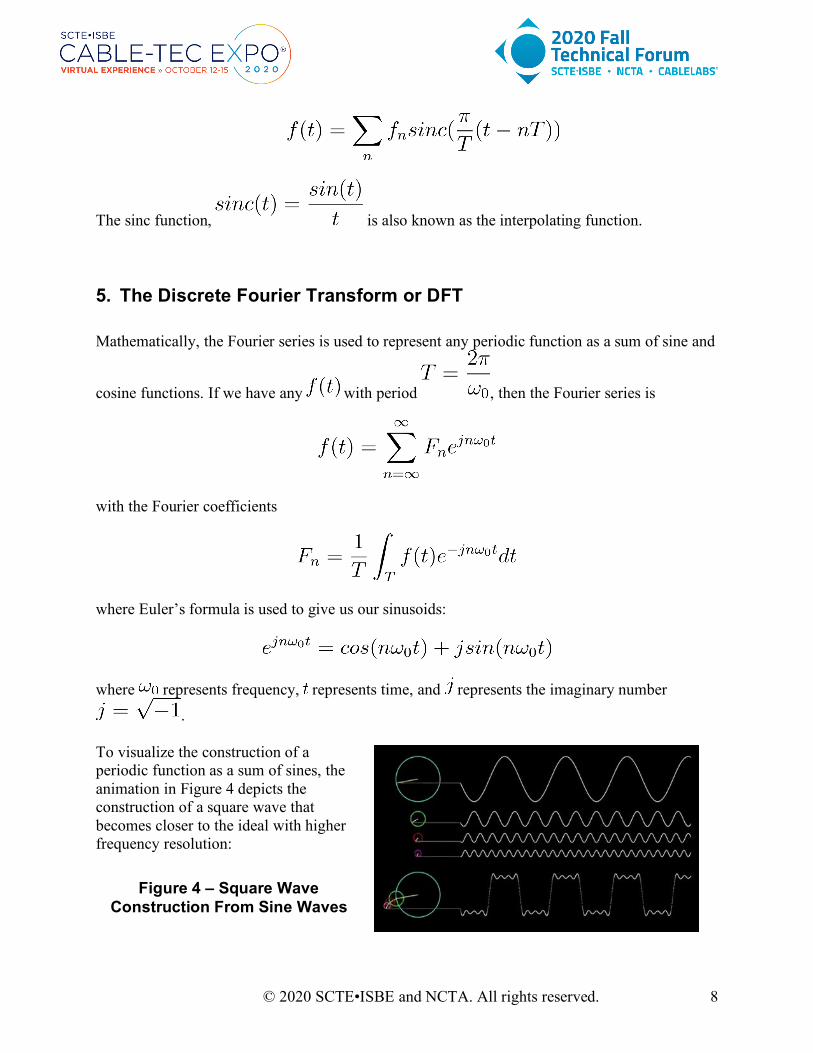
. To visualize the construction of a periodic function as a sum of sines, the animation in Figure 4 depicts the construction of a square wave that becomes closer to the ideal with higher frequency resolution:

Figure 4 – Square Wave Construction From Sine Waves

© 2020 SCTE•ISBE and NCTA. All rights reserved. 9

If a function is aperiodic, it can still be represented as a sum of sinusoids, but the frequencies of the sinusoids are no longer simply harmonics of a fundamental . A general aperiodic signal consists of a continuous spectrum of frequencies, so rather than integrating over a single period of as is the case with Fourier series coefficients, we must integrate over all time to derive the exact Fourier transform, which is the equivalent to the Fourier series coefficients but

in a continuous frequency range. In the limit as the period approaches infinity in an aperiodic signal, then the fundamental frequency approaches 0, and so we must integrate over the entire period of an aperiodic signal, which in other words, means we integrate over all time:

In analog signal processing, the Fourier transform is used to determine the characteristics of the signal in the frequency domain. We can determine the frequencies or spectral content present in using the Fourier transform, and manipulate or filter the signal as needed in the frequency domain. Then, we can use an inverse Fourier transform to go back to the original time domain function from the frequency domain:

Similarly, in digital signal processing, the discrete-time Fourier transform (DTFT) is used in order to convert a continuous discrete-time signal (input sequence) into its counterpart in the continuous frequency domain. It is modeled by the equation

where represents a discrete-time input signal, and is an integer. The inverse DTFT is given by

© 2020 SCTE•ISBE and NCTA. All rights reserved. 10

Finally, the discrete Fourier transform (DFT) is simply a “sampling” of the DTFT in the frequency domain – a finite version of the DTFT taken over a specified interval or number of samples. It is modeled by the equation

where N represents the total number of samples. And we can also define the inverse DFT by:

The DFT is a mainstay in the digital signal processing toolbox. It allows us to determine the spectral components of a sampled signal and to determine the frequency response of a system given the impulse response of the system in a completely digital manner. It uses a finite number of samples which can be easily used in computations of all kinds. The FFT, or fast Fourier transform, is an algorithm that is used to calculate the DFT in a mathematically efficient manner. The FFT is employed by mathematicians, engineers, musicians, and scientists to rapidly analyze, modify, or utilize sampled signals in the frequency domain for myriad applications. 6. Introduction to Profile Management Application The next two sections of this paper provide examples of using SDR to generate impairments for profile management application testing. A brief overview of PMA will demonstrate how highly customizable impairment profiles can aid in OFDM profile management testing. A profile management application system builds an optimized set of OFDM channel modulation profiles based on current plant conditions. It does this by collecting receive modulation error ratio data from cable modems, analyzing this data to sort modems into impairment groups, and finally building the modulation profiles and applying them on the CMTS (see Figure 5). The modulation profiles themselves typically contain variable bit-loaded regions ranging from excluded regions (0-QAM) for highly impaired subcarriers, to 4096-QAM in the low noise areas of the OFDM channel. In this way, the PMA algorithm is able to maximize overall channel capacity while maintaining robust profiles that are noise-tolerant.

© 2020 SCTE•ISBE and NCTA. All rights reserved. 11

Figure 5 – The Profile Management Application System

Laboratory RF environments are often very clean, with short cable runs, limited ingress, and few taps or active elements such as amplifiers or line extenders. To test profile recommendations generated by the PMA algorithm (Figure 6) we will need to introduce impairments with variable power levels, widths, and durations. The following sections demonstrate how software-defined radio can be used to create these impairments.

Figure 6 – PMA In Action: Building Custom OFDM Profiles

© 2020 SCTE•ISBE and NCTA. All rights reserved. 12

7. Practical Application Example #1– Capturing LTE Signals For

Replay as an Impairment Source Problem Statement: How can we capture LTE signals and introduce them as ingress interference in a laboratory environment? SDR Solution Outline:

1. Using a cellular telephone as a signal source, find the LTE band currently in use 2. Prepare the SDR to capture at the LTE uplink frequency 3. Start a speed test on the UE to generate traffic 4. Observe/capture the LTE signal on the SDR 5. Combine SDR TX into the lab RF plant and playback capture file 6. Observe effect in the cable modem’s downstream OFDM channel and verify PMA

OFDM channel profile recommendation

Detailed Steps: 1. Most modern UE devices include hidden service menu interfaces that can be accessed by

dialing certain sequences. For example: a. Apple iPhone (all): *3001#12345#* b. Samsung (Android): *#*#197328640#*#*or *#0011# c. Sony (Android): *#*#*386#*#* or *#*#*585*0000#*#* d. HTC (Android): *#*#7262626#*#*

Figure 7 - Finding LTE Band In Use on iPhone

From the above example, we can determine what uplink frequencies are assigned to Band 66:

© 2020 SCTE•ISBE and NCTA. All rights reserved. 13

Table 1 – LTE Frequency Bands (3)

2. Osmocom_fft is a simple spectrum analyzer and capture tool that can be used to write sampled data directly to a file. Using a command such as: osmocom_fft -f 1.89e9 -s 40.96e6 will launch the application and tune to 1.89 GHz. If the Osmocom utilities are not available, a GNU Radio Companion flowgraph can be created to output the data from a UHD:USRP source to a file sink block. The RX port of the SDR should be fitted with an antenna capable of receiving the LTE frequencies, such as a mini GSM/cellular quad-band antenna with 2 dBi of gain and 50 ohm impedance.

3. Install Speed test on the UE LTE source, disable Wi-Fi, and begin a speed test. Most testing includes a downlink and an uplink speed test portion. If the energy is not seen at the expected frequency, the downlink test may not have completed or the UE may have changed bands or moved to a neighboring macro cell.

4. The LTE signal should now be see on the analyzer. For live, raw IQ capture, Gqrx is a free open-source software-defined radio receiver that supports many popular radios including Airspy, rtl-sdr, HackRF, and USRP devices.

© 2020 SCTE•ISBE and NCTA. All rights reserved. 14

Figure 8 - Real Time Spectrum Analyzers for IQ Capture (clockwise):

osmocom_fft, uhd_fft, gqrx SDR

5. Combine the SDR TX Port 1 into the laboratory RF plant as needed to impact the desired

set of modems. For example:

Figure 9 - Combining of Noise Sources in Laboratory Environment

© 2020 SCTE•ISBE and NCTA. All rights reserved. 15

7. Through the splitting and combining network, different interference groups can be created. In this way the k-means based clustering algorithm that the PMA analytics engine implements can be fully tested, as multiple, custom OFDM channel profiles are supported.

8. Practical Application Example #2 – How SDR Has Aided Profile Management Application (PMA) Testing

Problem Statement: How can we re-create an OFDM channel impairment profile using a cable modem’s reported RxMER values? SDR Solution Outline:

1. Read in cable modem RxMER data file 2. Convert the data from ¼ dB values to dB 3. To create the impairment profile, set all values that are within a threshold (say 6-10 dB)

of the maximum value to zero. We will be using the values outside of this “good” range to create our impairment.

4. Convert the RxMER value from a ratio of power values to output voltage for the DAC 5. Normalize the voltage value vector 6. Use GNU Radio to stream out the data to an inverse fast Fourier transform block to

convert from frequency to time domain 7. Stream the data to either a file to use for later playback, or directly to the software-

defined radio sink 8. Inject this RF impairment into the lab environment physical plant to re-create the

impairment seen at the customer premises

Detailed Steps: 1. The cable modem RxMER values can be obtained either directly from CMTS CLI or via

TFTP download. The values are reported in quarter-dB, for example:

0x0000 00000000 00000000 00000000 00000000 00000000 00000000 00000000 00000000 0x0020 00000000 00000000 00000000 00000000 00000000 00000000 00000000 00000000 0x0040 00000000 00000000 00000000 00000000 00000000 00000000 00000000 00000000 0x0060 00000000 00000000 00000000 00000000 00000000 00000000 00000000 00000000

.

.

. 0x0400 00000000 00000000 00000000 00000000 00000000 00000000 00000000 00000000 0x0420 00000000 00000000 00000000 00000000 00000000 00000000 00000000 00000000 0x0440 00000000 00000000 00000000 00000000 00000000 00000000 00000000 00000000 0x0460 00000000 0000B6B7 B9B6BCB6 B5BABAB4 B6B3B4B5 BAB3B8B3 BAB6B8B5 B5BBBBB6 0x0480 B6BAB5B9 B9B7BBB7 BCB4B4BA B4B6B7B9 B6B8B3BD B7B7B8B5 B8B8B8B6 B7B8B7B9 0x04A0 BAB3B8B5 B6B7B8B8 BCB7B8BB B8BAB4B8 B7B6B9B3 B6B9B9B8 B7B9B9B9 B4BCBAB5 0x04C0 B6B8B4B7 B7BAB8B8 B3B8B7B4 B8B6B7B9 B9B4B8B5 B9BAB6B9 B4B6B4B9 B4B6B9BA 0x04E0 B6B9B3B7 BAB2B5B6 B5B5B4B6 B4B7B7BA B9B7B5BA B9B6B9B4 B6B7B7B7 BDBAB6B3 0x0500 B6B6B4B7 B6BABBBC B3B8B5B7 B7B7B5BB B6B6B6B8 B7B7B6BA B4B6B8B9 B7B5B8B7 0x0520 B9B6B5B8 B3B9B7B6 B6BBB7B5 B8B9B4B7 B8B7B4B7 B7B7B8BA B8B7B5B4 B4B4B9B3

.

.

. 0x0F40 00000000 00000000 00000000 00000000 00000000 00000000 00000000 00000000 0x0F60 00000000 00000000 00000000 00000000 00000000 00000000 00000000 00000000

© 2020 SCTE•ISBE and NCTA. All rights reserved. 16

0x0F80 00000000 00000000 00000000 00000000 00000000 00000000 00000000 00000000 0x0FA0 00000000 00000000 00000000 00000000 00000000 00000000 00000000 00000000 0x0FC0 00000000 00000000 00000000 00000000 00000000 00000000 00000000 00000000 0x0FE0 00000000 00000000 00000000 00000000 00000000 00000000 00000000 00000000

If using the values from the TFTP downloaded RxMER file, the RxMER per subcarrier data follows after a header using the specified format:

Table 2 – RxMER TFTP File Format (4)

The other data such as the subcarrier zero frequency, first active subcarrier index, subcarrier spacing, and length in bytes of the RxMER data will all be used to fully describe the OFDM channel impairment profile.

2. The RxMER data itself is defined as the ratio of the average power of the ideal QAM constellation to the average error-vector power. The error vector is the difference between the equalized received pilot or preamble value and the known correct pilot value or preamble value. The reported values are represented in hexadecimal values of ¼ dB. Multiple each value in the array by ¼ to properly scale.

3. In this step we discard (set to zero) all values that are within a configurable threshold of the maximum reported RxMER value. Only the low RxMER values will be used to construct the impairment vector. This example used a value of 10 dB.

4. Convert every value in the impairment array to an output voltage value for the DAC using the formula: V = 10 (dB/20)

5. Divide every voltage value by the sum of values (new values will all sum to 1) to avoid overloading the SDR output stage.

6. The processing of the RxMER data, along with the streaming to either file or directly to the software-define radio sink was achieved through the creation of a GNU Radio Companion flowgraph (Figure 10).

© 2020 SCTE•ISBE and NCTA. All rights reserved. 17

Figure 10 - GRC Flowgraph to Contruct and Transmit Custom Impairment

Waveform

Flowgraph Details: Embedded Python Module- The previous six steps were all done in the embedded Python Module block. GNU Radio companion allows you to create and use custom Python code within your flowgraph. In this example, all the RxMER data manipulation and plot generation was done within the embedded Python block. After reading in the modem’s RxMER data, the values are written to disk as a Matplotlib Pyplot (Figure 11):

© 2020 SCTE•ISBE and NCTA. All rights reserved. 18

Figure 11 - Graph of RxMER Data Generated by Embedded Python Block

Vector Source Block - This flowgraph begins with the vector source block. This block streams items based on the input vector, which in this case is the output of a Python method in our embedded Python block. Throttle Block - This stream feeds a throttle block. This block will be set to “bypass” when using the real SDR hardware which will set its own sampling rate. It is used in combination with the software sinks or file output, when the sampling rate would only be determined by the host’s CPU clock. Stream to Vector Block – This block converts the stream of items into a stream of vectors containing N number of items. In this case the number of items will be the FFT size (4096). The stream-to-vector and vector-to-stream blocks are special in that the input and output types differ by a decimation or interpolation factor. In our example, the stream-to-vector block produces one output vector for every 4096 input samples. FFT Block – The complex valued output vector from the previous stage feeds the fast Fourier transform block. The key parameters of the FFT block are: FFT size (number of samples used in each FFT calculation), direction (forward for FFT, reverse for inverse FFT), window, shift (puts DC – 0 Hz – in the center of the FFT block for complex input type), and number of threads. Vector to Stream Block – The output of the FFT block will always be complex-valued. This block will convert a stream of vectors from the FFT block to a stream of items that can be fed directly to an output file, the

© 2020 SCTE•ISBE and NCTA. All rights reserved. 19

SDR hardware, a GUI frequency sink that offers spectrum analyzer functionality, or a Fosphor or Waterfall sink for more real-time spectrum analyzer-like output.

Figure 12 - Qt GUI Frequency Sink Visualization of Impairment Signal

Figure 13 - Qt Fosphor Sink Visualization of Impairment Signal

© 2020 SCTE•ISBE and NCTA. All rights reserved. 20

Rational Resampler Block – If trying to stream a file that has been sampled at a rate that is not supported by the SDR hardware, the rational resampler block allows us to change the sampling rate (e.g., from the DOCSIS standard 204.8 MHz). In this example the default hardware sampling rate is 245.76 MHz so we could set the interpolation factor to 6 and the decimation factor to 5 to upsample to 245.76 MHz.

7. If the output is sent to a file, we can replay directly to the SDR sink without continuously performing the IFFT calculation repeatedly. The act of streaming 32 bit IQ data at 245.76 MHz is very I/O intensive and requires a powerful host computer with a 10 gigabit interface. As seen in Figure 14 this stream from the host to the SDR hardware averages around ~7.8 Gbps:

Figure 14 - Bandwith Monitor of IQ Data Stream

8. The SDR TX output can then be combined into the laboratory plant, and the effect can then be observed in the OFDM channel RxMER data (Figure 15).

© 2020 SCTE•ISBE and NCTA. All rights reserved. 21

Figure 15 - Impairment Signal on Spectrum Analyzer

In this case we were testing the response of our profile management application (a.k.a. Octave) to verify that proper bitloading values were being set for the impacted frequency ranges. For an example OFDM profile, see Figure 16.

DS DS Low-High Freq Bits/Symbol/ MaxRate S/C/CH Prof Edge (MHz.KHz) Mod Subcarrier Mb/sec

9/0/48 0 -default- 256qam 8.00 584 9/0/48 1 -default- 4096qam 11.73 856 9/0/48 1 702.000-708.000 2048qam - - 9/0/48 1 735.000-737.000 2048qam - - 9/0/48 1 738.000-744.000 2048qam - - 9/0/48 1 745.000-756.000 2048qam - - 9/0/48 2 -default- 4096qam 10.75 785 9/0/48 2 795.000-801.000 1024qam - - 9/0/48 2 802.000-813.000 512qam - - 9/0/48 2 816.000-828.000 512qam - - 9/0/48 2 831.000-832.000 2048qam - -

.

.

.

Figure 16 - OFDM Profile for SDR Generated Impairment Signal

© 2020 SCTE•ISBE and NCTA. All rights reserved. 22

9. Equipment Used Software-Defined Radio Hardware:

1. Ettus Research USRP N320 2. Ettus Research USRP B210 Mini 3. Great Scott Gadgets HackRF One 4. 75 MHz to 1 GHz telescoping antenna 5. SMA Make Right Angle antenna (850/900/1800/1900/2100 MHz, 2 dBi gain, 50 ohm) 6. 10 Gb direct-attach copper cables

Software-Define Radio Software:

1. GNU Radio v3.8.1.0 2. Ettus Research UHD drivers UHD_3.15.0.HEAD-0-gaea0e2de 3. GNU C++ v9.3.0 4. Python 3.8.2 5. Various libraries including libosmodsr-dev, libhackrf-dev, gr-osmosdr, gr-fosphor,

SDR Controller Host Computer:

• CPU - AMD Ryzen Threadripper 3970X • Motherboard - Asus ROG Zenith II Extreme Alpha • RAM – 32 GB Corsair DDR4 3600 • Storage – Samsung 970 EVO M.2 1 TB (x2) • GPU - EVGA GeForce RTX 2080 Ti Xc Hybrid 11 Gb DDR6 • Network – Asus XG-C100C 10G Network Adapter PCI-E x4 • Power – Thermaltake 1200 W 80+ Platinum

OS Software:

1. Ubuntu 20.04 LTS 2. Windows 10

Spectrum Analyzer:

• Siglent SSA 3021X Plus (9 kHz to 2.1 GHz)

© 2020 SCTE•ISBE and NCTA. All rights reserved. 23

10. Conclusion In this paper, we have explored what software-defined radio is and what it offers to engineers, students, and designers. We presented a general architecture as well as some needed background information on sampling theory and the discrete Fourier transform. Finally, the hardware, software, and drivers used to implement real data flows to sample and/or generate signals were detailed, along with two laboratory use cases. With the abundance of open-source community supported software and low cost hardware, software-defined radio is proving be a valuable laboratory and field testing tool. By abstracting the functionality from a specific piece of physical hardware, we can transmit and receive various modulation methods, perform signal processing and filtering, and customize routines though Python extensions all within a common software framework. These advantages, combined with the ability to embed Python code for customized signal processing routines, positions software-defined radio as a valuable laboratory and field testing tool.

© 2020 SCTE•ISBE and NCTA. All rights reserved. 24

Abbreviations

ADC analog-to-digital converter AWS advanced wireless service bps bits per second CLI command line interface CMTS cable modem termination system CPU central processing unit DAC digital-to-analog converter dB decibel dBi decibel isotropic DC direct current DFT discrete Fourier transform DSP digital signal processing DTFT discrete time Fourier transform FDD frequency division duplex (or duplexing) FFT fast Fourier transform FPGA field programmable gate array GB gigabyte GbE gigabit Ethernet Gbps gigabits per second GHz gigahertz GPSDO Global Positioning System disciplined oscillator GRC GNU Radio Companion GSM global system for mobile communications (originally groupe spécial

mobile) GUI graphical user interface Hz hertz IEEE Institute of Electrical and Electronics Engineers IF intermediate frequency IFFT inverse fast Fourier transform I/O input/output IQ in-phase/quadrature ISBE International Society of Broadband Experts kHz kilohertz LO local oscillator LTE long term evolution MHz megahertz MS/s megasamples per second OFDM orthogonal frequency division multiplexing OS operating system PCS personal communications service PMA profile management application PPS pulse per second

© 2020 SCTE•ISBE and NCTA. All rights reserved. 25

QAM quadrature amplitude modulation QSFP+ quad small form-factor pluggable plus RAM random access memory RF radio frequency RU rack unit RX receive (or receiver) RxMER receive modulation error ratio SCTE Society of Cable Telecommunications Engineers SDR software-defined radio SFP+ enhanced small form-factor pluggable SMA subminiature version A [connector] SoC system on a chip TFTP Trivial File Transport Protocol TX transmit (or transmitter) UE user equipment UHD USRP hardware driver USB universal serial bus USRP universal software radio peripheral

Bibliography & References

1. SDRF-06-R-0011-V1.0.0: SDRF Cognitive Radio Definitions 2. https://www.testandmeasurementtipe.com/temporal-spatioa-aliasing-signal-processing 3. ETSI TS 136 508 V15.5.0 LTE; Evolved Universal Terrestrial Radio Access (E-UTRA)

and Evolved Packet Core (EPC); Common test environments for User Equipment (UE) conformance testing

4. Cable Modem Operations Support System Interface Specification CM-SP-CM-OSSIv3.1-I17-200610