
RF COIL DESIGN FOR MULTI-FREQUENCY ... - Texas A&M...
87
RF COIL DESIGN FOR MULTI-FREQUENCY MAGNETIC RESONANCE IMAGING AND SPECTROSCOPY A Thesis by ARASH DABIRZADEH Submitted to the Office of Graduate Studies of Texas A&M University in partial fulfillment of the requirements for the degree of MASTER OF SCIENCE December 2008 Major Subject: Electrical Engineering
Transcript of RF COIL DESIGN FOR MULTI-FREQUENCY ... - Texas A&M...
RF COIL DESIGN FOR MULTI-FREQUENCY MAGNETIC RESONANCE
IMAGING AND SPECTROSCOPY
A Thesis
by
ARASH DABIRZADEH
Submitted to the Office of Graduate Studies of Texas A&M University
in partial fulfillment of the requirements for the degree of
MASTER OF SCIENCE
December 2008
Major Subject: Electrical Engineering

RF COIL DESIGN FOR MULTI-FREQUENCY MAGNETIC RESONANCE
IMAGING AND SPECTROSCOPY
A Thesis
by
ARASH DABIRZADEH
Submitted to the Office of Graduate Studies of Texas A&M University
in partial fulfillment of the requirements for the degree of
MASTER OF SCIENCE
Approved by:
Chair of Committee, Mary Preston McDougall Committee Members, Steven M. Wright Chin B. Su Melissa A. Grunlan Head of Department, Costas Georghiades
December 2008
Major Subject: Electrical Engineering
iii
ABSTRACT
RF Coil Design for Multi-Frequency Magnetic Resonance Imaging and Spectroscopy.
(December 2008)
Arash Dabirzadeh, B.Sc., Amirkabir University of Technology (Tehran Polytechnic)
Chair of Advisory Committee: Dr. Mary Preston McDougall
Magnetic Resonance Spectroscopy is known as a valuable diagnostic tool for
physicians as well as a research tool for biochemists. In addition to hydrogen (which is
the most abundant atom with nuclear magnetic resonance capability), other species (such
as 31P or 13C) are used as well, to obtain certain information such as metabolite
concentrations in neural or muscular tissues. However, this requires nuclear magnetic
resonance (NMR) transmitter/receivers (coils) capable of operating at multiple
frequencies, while maintaining a good performance at each frequency. The objective of
this work is to discuss various design approaches used for second-nuclei RF (radio
frequency) coils, and to analyze the performance of a particular design, which includes
using inductor-capacitor (LC) trap circuits on a 31P coil. The method can be easily
applied to other nuclei. The main advantage of this trapping method is the enabling
design of second-nuclei coils that are insertable into standard proton coils, maintaining a
near-optimum performance for both nuclei. This capability is particularly applicable as
MRI field strengths increase and the use of specialized proton coils becomes more
prevalent. A thorough performance analysis shows the benefit of this method over other

iv
designs, which usually impose a significant signal-to-noise (SNR) sacrifice on one of the
nuclei.
A methodology based on a modular coil configuration was implemented, which
allowed for optimization of LC trap decoupling as well as performance analysis. The 31P
coil was used in conjunction with various standard 1H coil configurations
(surface/volume/array), using the trap design to overcome the coupling problem
(degraded SNR performance) mentioned above. An analytical model was developed and
guidelines on trap design were provided to help optimize sensitivity. The performance
was analyzed with respect to the untrapped case, using RF bench measurements as well
as data obtained from the NMR scanner. Insertability of this coil design was then
verified by using it with general-purpose proton coils available. Phantoms were built to
mimic the phosphorus content normally found in biologic tissues in order to verify
applicability of this coil for in vivo studies. The contribution of this work lies in the
quantification of general design parameters to enable “insertable” second-nuclei coils, in
terms of the effects on SNR and resonance frequency of a given proton coil.
v
ACKNOWLEDGEMENTS
I would like to thank all my teachers, professors, and mentors who have helped
form my understanding of science and engineering throughout the years. Special thanks
to all my committee members; my committee chair, Dr. Mary McDougall, who is an
inspiration of hard work and maintaining high standards, Dr. Steve Wright, who has
dedicated his knowledge and expertise to the business of saving lives. Thanks to the
personnel of Philips Invivo Corp. especially Dr. Charles Saylor and Dr. Arne
Reykowski. Also I would like to acknowledge my labmates, for their companionship
during long days.
Thanks also go to all my friends for making the last couple of years a great
experience. Last, but not the least, thanks to my parents who have dedicated their lives to
culture and education and to my older brother whose never-ending support and
encouragement got me where I am standing today.

vi
TABLE OF CONTENTS
Page
ABSTRACT .............................................................................................................. iii
ACKNOWLEDGEMENTS ...................................................................................... v
TABLE OF CONTENTS .......................................................................................... vi
LIST OF FIGURES ................................................................................................... viii
LIST OF TABLES .................................................................................................... xi
CHAPTER
I INTRODUCTION ................................................................................ 1 I.1 NMR Spectroscopy ................................................................... 1 I.2 NMR Physics ............................................................................ 2 I.3 RF Coils .................................................................................... 5 I.4 Multi-frequency Applications and Motivation ......................... 8 I.5 Multiple-frequency RF Coils .................................................... 10 I.6 Importance of Insertability ........................................................ 11 II METHODS FOR DUAL-TUNING COILS ........................................ 13 II.1 Single-Coil Approach .............................................................. 13 II.1.1 Dual-tuning a Coil Using Lumped-element Traps ...... 13 II.1.2 Dual-tuning a Coil Using Isolation Filters .................. 19 II.2 Dual Coil Approach ................................................................ 24
III USING TRAPS IN DUAL-COIL DESIGNS ...................................... 30 III.1 Tank Circuits .......................................................................... 30 III.2 Coil Implementation ............................................................... 32 III.3 Coupling Effects ..................................................................... 34 III.3.1 Initially Tuned Degenerate ......................................... 35 III.3.2 Initially Tuned to Separate Frequencies ..................... 36 III.4 Bench Measurement Results .................................................. 38 III.5 SNR Model ............................................................................. 45 III.5.1 B1 Magnitude .............................................................. 45

vii
CHAPTER Page
III.5.2 Noise Level ................................................................ 50 IV MRI/MRS TESTING ........................................................................... 54 IV.1 Spectroscopy Using the Varian Inova System ....................... 54 IV.1.1 System Modifications ................................................ 54 IV.1.2 Shimming ................................................................... 55 IV.1.3 Effect of Averaging (transients) ................................. 60 IV.1.4 Exponential Line-broadening (apodization) Filters ... 61 IV.2 Trap Analysis ......................................................................... 62 IV.2.1 Comparison Methodology .......................................... 62 IV.2.2 Results: Spectra .......................................................... 64 IV.2.3 Results: Proton Imaging ............................................. 65 IV.3 Insertability ............................................................................ 66 V CONCLUSIONS AND FUTURE WORK .......................................... 71 REFERENCES .......................................................................................................... 73
VITA ......................................................................................................................... 76
viii
LIST OF FIGURES
Page Figure I-1 Magnetic field on the axis of a circular loop ................................ 7 Figure I-2 Effect of proton decoupling on phosphorus spectrum .................. 9 Figure I-3 Two examples of concentric coil design ....................................... 11 Figure II-1 Impedance model for a RF coil ..................................................... 14 Figure II-2 Resonance model for a dual-tuned coil ......................................... 14 Figure II-3 Reactance of a single-tuned coil and a trap .................................. 16 Figure II-4 Single-input dual-tuned coil .......................................................... 18 Figure II-5 Dual-tuned single-coil with two input ports ................................. 19 Figure II-6 Dual-tuned single coil with two isolated inputs ............................ 21 Figure II-7 Dual-tuned single coil for 13C and 1H ........................................... 22 Figure II-8 Lumped-element shunt isolation filters ........................................ 23 Figure II-9 Equivalent circuit for two loss-less coupled coils ........................ 25 Figure II-10 Two coil designs producing a magnetic field parallel to their plane ............................................................ 27 Figure II-11 Half-volume quadrature dual-tuned coil design ........................... 29 Figure III-1 Non-ideal LC trap circuit .............................................................. 31 Figure III-2 Real and imaginary parts of non-ideal trap impedance ................ 32 Figure III-3 Concentric surface coil structure .................................................. 33 Figure III-4 Equivalent circuit diagram of two degenerate coils placed near each other ........................................ 35
ix
Page Figure III-5 Effect of coil coupling between 1H coil and 31P coil at 4.7T, manifesting itself as a shift in the desired resonance frequency ......................................................... 38 Figure III-6 Screenshot from Agilent 5071 network analyzer showing the effect of the 31P coil on 1H resonance frequency(shift of 8 MHz) ......... 39 Figure III-7 Effect of 31P coil on 1H field intensity .......................................... 41 Figure III-8 Proton field magnitude across the coil .......................................... 43 Figure III-9 Q factor of the inductor (22nH) used to make the trap ................. 44 Figure III-10 Coupled dual-tuned resonators ..................................................... 45 Figure III-11 Effect of 31P coupling in 1H coil field strength along the axis .... 47 Figure III-12 Coupled dual-tuned resonators with a trap included .................... 48 Figure III-13 Effect of the trap Q on proton field magnitude ............................. 49 Figure III-14 Effect of the trap inductor value on coil performance .................. 52 Figure III-15 Effect of the trap Q value on coil performance ............................ 53 Figure IV-1 1H spectra obtained to measure linewidth after shimming ........... 56 Figure IV-2 The three-chamber phantom used for spectroscopy ..................... 57 Figure IV-3 Sample spectra obtained from the physiological phosphorus phantom .............................................. 57 Figure IV-4 Effect of power on spectra obtained from an inhomogeneous phantom ......................................................... 59 Figure IV-5 Maximum signal over pulsewidths ranging from 20 to 400 µs used for 90 degree pulsewidth calibration ...... 60 Figure IV-6 Effect of averaging on spectra ...................................................... 61 Figure IV-7 Effect of time-domain filtering on spectra .................................... 62
x
Page Figure IV-8 31P spectra obtained with Left: no trap in place Right: with trap in place ................................................................ 65 Figure IV-9 Images obtained from (a): proton coil with no 31P coil present. (b): proton coil with untrapped 31P coil present. (c) proton coil after adding the trap on the 31P coil .............................................. 66 Figure IV-10 The surface phosphorus coil being used with a proton volume coil .................................................... 67 Figure IV-11 Images obtained from a proton volume coil. (a) no 31P coil present (b) untrapped 31P coil present, showing reduced sensitivity (c) trapped 31P coil present ............................................................ 68 Figure IV-12 Three-element phased-array proton coil structure ........................ 69

xi
LIST OF TABLES
Page
Table 1 NMR properties for some common nuclei ................................... 3
Table 2 Resonance frequency and distributed capacitor values used in each coil ................................................. 34
Table 3 Relative SNR obtained at different configurations ....................... 68
Table 4 Effect of the 31P coil on element coupling for the proton array coil ................................................................ 70
1
CHAPTER I
INTRODUCTION1
I.1. NMR Spectroscopy
Nuclear magnetic resonance (NMR) spectroscopy has long been used in
chemistry and more recently in molecular/metabolic medicine. With the increasing
availability of whole-body high field-strength magnets for magnetic resonance imaging
(MRI), non-proton spectroscopy is finding new promise as a diagnostic tool. Among
nuclei with NMR capability, 13C and 31P have been of particular interest. 13C found in
organic compounds is used extensively in metabolic studies such as glucose labeling,
and proton-decoupled magnetic resonance spectroscopy (MRS) of 31P (which comprises
100% of phosphorus content), has diagnostic importance in ischemic cardiac
myopathy[1] [2], a variety of brain disease[3], and also in monitoring effectiveness of
cancer treatment procedures[4] [5]. Phosphorus metabolites, such as adenosine
triphosphate (ATP) and phosphocreatine (PCr), are involved in reactions regulating
energy delivery to the cells, as it is the equilibrium between the two that responds to a
sudden rise in energy demand in muscular tissues. Advances in the design of
spectrometers and MRI scanners are enabling in vivo interrogation of biological samples
in animal and human studies.
This thesis follows the style of Journal of Magnetic Resonance.
2
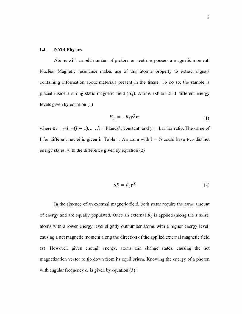
I.2. NMR Physics
Atoms with an odd number of protons or neutrons possess a magnetic moment.
Nuclear Magnetic resonance makes use of this atomic property to extract signals
containing information about materials present in the tissue. To do so, the sample is
placed inside a strong static magnetic field ( ). Atoms exhibit 2I+1 different energy
levels given by equation (1)
(1)
where , 1 , … , Planck’s constant and Larmor ratio. The value of
I for different nuclei is given in Table 1. An atom with I = ½ could have two distinct
energy states, with the difference given by equation (2)
∆ (2)
In the absence of an external magnetic field, both states require the same amount
of energy and are equally populated. Once an external is applied (along the z axis),
atoms with a lower energy level slightly outnumber atoms with a higher energy level,
causing a net magnetic moment along the direction of the applied external magnetic field
(z). However, given enough energy, atoms can change states, causing the net
magnetization vector to tip down from its equilibrium. Knowing the energy of a photon
with angular frequency is given by equation (3) :
3
(3)
The frequency of a time-varying electromagnetic field required to cause the energy level
transition is given by equation (4)
(4)
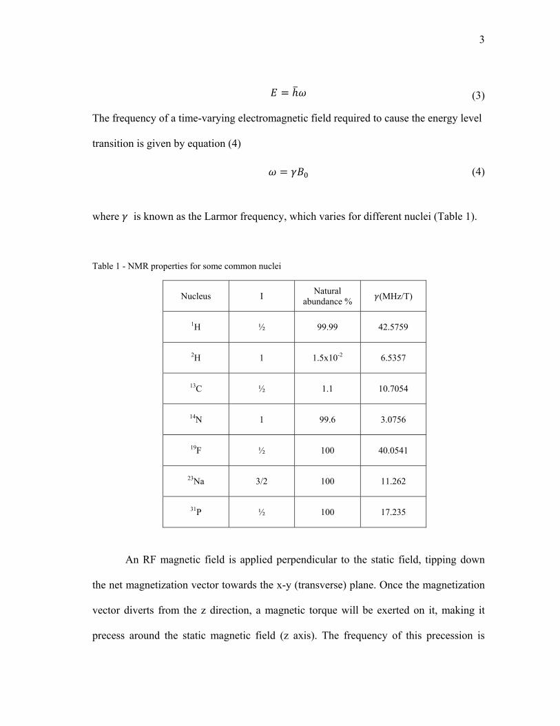
where is known as the Larmor frequency, which varies for different nuclei (Table 1).
Table 1 - NMR properties for some common nuclei
Nucleus I Natural abundance % (MHz/T)
1H ½ 99.99 42.5759
2H 1 1.5x10⁻² 6.5357
13C ½ 1.1 10.7054
14N 1 99.6 3.0756
19F ½ 100 40.0541
23Na 3/2 100 11.262
31P ½ 100 17.235
An RF magnetic field is applied perpendicular to the static field, tipping down
the net magnetization vector towards the x-y (transverse) plane. Once the magnetization
vector diverts from the z direction, a magnetic torque will be exerted on it, making it
precess around the static magnetic field (z axis). The frequency of this precession is
4
known to be the same as Larmor frequency. Once the magnetization, or some portion of
it, reaches the x-y plane, the RF field is cut off, allowing the magnetization to relax back
to the z direction, releasing the RF energy that was just applied to it. The frequency of
this RF signal is the same as the precession frequency, and the amplitude of this RF
signal is proportional to the magnitude of the transverse portion of the magnetization
vector.
NMR imaging uses space-varying static magnetic fields, known as gradient fields
to frequency encode the spatial information into the resultant RF signal. Remember that
the Larmor frequency is proportional to the static field . So if we have a different
magnetic field at each location, spins in different locations will precess at different
frequencies. Because of the superposition principle, signals from different locations add
up to the resultant RF signal, the frequency content of which corresponds to the extent of
the sample. By taking the Fourier transform of this signal, we can find signal amplitude
at each location, i.e. a projection image.
When this spatial localization is not implemented, the basic principle in use are
those of NMR spectroscopy, used by chemists to identify unknown materials or
concentration of certain compounds present in a sample. Different chemical compounds
within the sample have slightly different values than reference nuclei, (because of
bonds to other atoms in the molecular structure), so they will precess at different
frequencies. Frequency offset from the reference frequency is known as chemical shift,
defined as:

5
The Fourier transform of the detected signal will give us the spectrum, showing peaks at
certain frequencies. By mapping these to the table of chemical shifts, chemists can
identify compounds present in the sample.
Molecular bonds not only change the Larmor frequency of the atom, they might
also cause it to split into two frequencies; known as spin coupling. In this case, the
resonance frequency of an atom will be dependent on the energy state of the
neighboring, coupled atoms. This is especially true for bonds to hydrogen, in carbon and
phosphorus compounds. Because of the low abundance of 13C and phosphorus, splitting
can further attenuate the signal, making it difficult to read. In order to overcome this
problem, we need to “decouple” the hydrogen magnetization from our nuclei of interest
(carbon or phosphorus). This is usually done via a saturation pulse. A high-power RF
pulse at the hydrogen frequency is applied for a long time, usually on the order of 1 s,
until the average hydrogen magnetization disappears. Then, the original signal of interest
is read out. In this manner, hydrogen atoms will no longer affect carbon or phosphorus
resonance frequencies.
I.3. RF Coils
Transmission of an oscillating magnetic field, and detection of the resultant RF
signal, is done via RF coils, or resonators. In transmit mode, a high-power RF amplifier
is applied to the coil terminals, forming a current distribution on the coil conductors.
This current generates a magnetic field ( ) oscillating at the RF input frequency.
6
In receive mode, the magnetization vector within the sample is precessing,
causing a flux change through the coil, inducing an electro-motive force (EMF) in the
coil (Faraday induction). By amplifying this signal and taking the FFT, we have our
spectrum.
Surface coils are the simplest form of RF coils used to produce/detect magnetic
field. They usually provide better SNR than volume coils; since a smaller portion of the
sample contributes to the received noise level; however the magnetic field
inhomogeneity of surface coils can be a disadvantage.
The Biot-Savart law is commonly used as an analytical model to describe the
magnetic field produced by an electric current. If we define a differential element of
steady current (using the standard prime notation to mark the source variables) as
and integrate over the current path, the vector magnetic potential [5] is found using
equation (5) :
4 (5)
and the magnetic field will be
4 (6)
where is the unit displacement vector between the current element (source) and the
observation point, and is the distance between the two. The electric field can be found
using equation (7)
7
(7)
where is the electric potential, contributing as a conservative electric field. Note that in
this model (known as the quasi-static model), effect of the time-varying electric field on
the magnetic field is ignored.
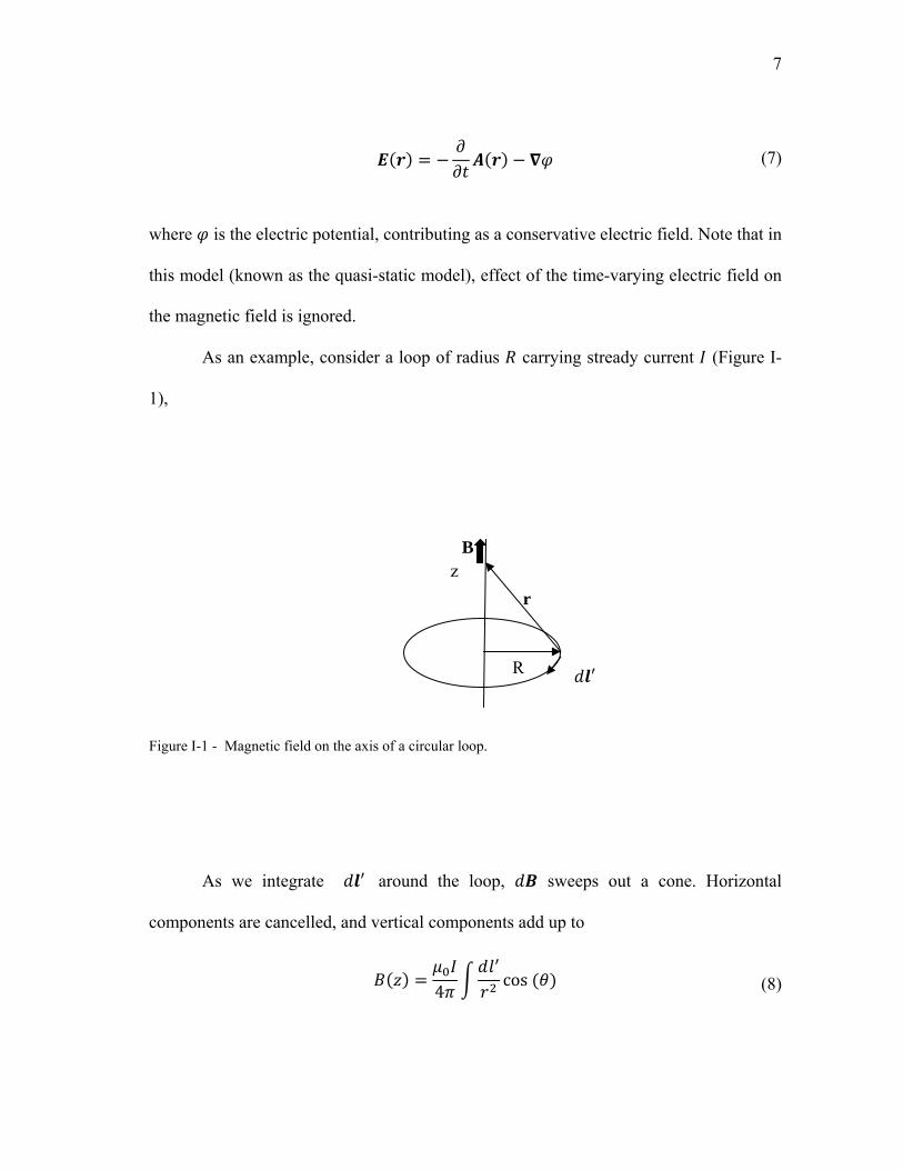
As an example, consider a loop of radius carrying stready current (Figure I-
1),
As we integrate around the loop, sweeps out a cone. Horizontal
components are cancelled, and vertical components add up to
4 cos (8)
r
R
B
z
Figure I-1 - Magnetic field on the axis of a circular loop.
8
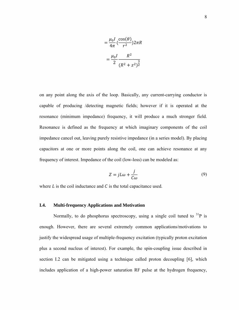
4cos
2
2
on any point along the axis of the loop. Basically, any current-carrying conductor is
capable of producing /detecting magnetic fields; however if it is operated at the
resonance (minimum impedance) frequency, it will produce a much stronger field.
Resonance is defined as the frequency at which imaginary components of the coil
impedance cancel out, leaving purely resistive impedance (in a series model). By placing
capacitors at one or more points along the coil, one can achieve resonance at any
frequency of interest. Impedance of the coil (low-loss) can be modeled as:
(9)
where is the coil inductance and is the total capacitance used.
I.4. Multi-frequency Applications and Motivation
Normally, to do phosphorus spectroscopy, using a single coil tuned to 31P is
enough. However, there are several extremely common applications/motivations to
justify the widespread usage of multiple-frequency excitation (typically proton excitation
plus a second nucleus of interest). For example, the spin-coupling issue described in
section I.2 can be mitigated using a technique called proton decoupling [6], which
includes application of a high-power saturation RF pulse at the hydrogen frequency,
9
applied long enough for proton magnetization to disappear, thus removing its splitting
effect on phosphorus resonances. For some molecules, phosphorus spectra are of little
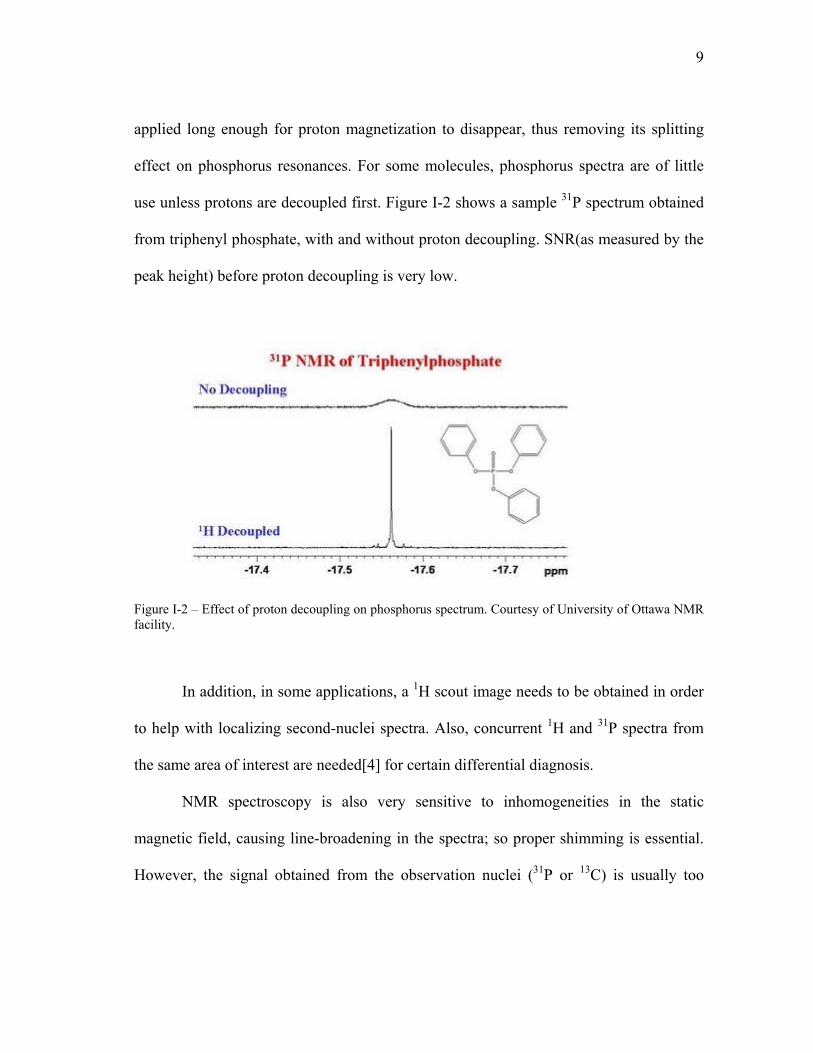
use unless protons are decoupled first. Figure I-2 shows a sample 31P spectrum obtained
from triphenyl phosphate, with and without proton decoupling. SNR(as measured by the
peak height) before proton decoupling is very low.
Figure I-2 – Effect of proton decoupling on phosphorus spectrum. Courtesy of University of Ottawa NMR facility.
In addition, in some applications, a 1H scout image needs to be obtained in order
to help with localizing second-nuclei spectra. Also, concurrent 1H and 31P spectra from
the same area of interest are needed[4] for certain differential diagnosis.
NMR spectroscopy is also very sensitive to inhomogeneities in the static
magnetic field, causing line-broadening in the spectra; so proper shimming is essential.
However, the signal obtained from the observation nuclei (31P or 13C) is usually too
10
weak for shimming. A proton channel is therefore usually used to shim the static
magnetic field in the region of interest.
In the case of low-abundant nuclei (such as 13C), a technique based on the
Nuclear Overhauser Effect has been used to polarize proton spins and then transfer it to
carbon spin population[7].
All of these applications require some way of exciting spins at two frequencies
over the same region of interest.
I.5. Multiple-frequency RF Coils
Because of this need for multi-frequency excitation (described in section I.4), it
is worthwhile to examine the various possible design approaches for this task. In multi-
nuclear applications, two nuclear species are interrogated; such as 1H and 31P. The coil
system needs to generate/detect RF magnetic field at two different frequencies; namely
200.23 MHz and 81.05 MHz for the case of 1H and 31P at 4.7 T. One method, a single-
coil approach, uses inherently multiple-mode resonant structures.
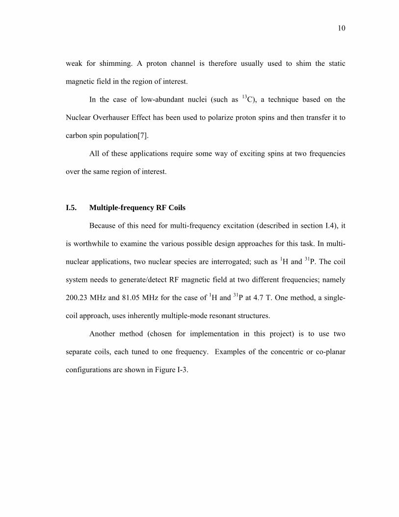
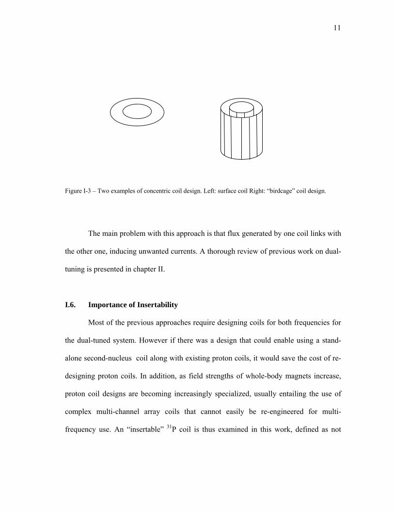
Another method (chosen for implementation in this project) is to use two
separate coils, each tuned to one frequency. Examples of the concentric or co-planar
configurations are shown in Figure I-3.
11
The main problem with this approach is that flux generated by one coil links with
the other one, inducing unwanted currents. A thorough review of previous work on dual-
tuning is presented in chapter II.
I.6. Importance of Insertability
Most of the previous approaches require designing coils for both frequencies for
the dual-tuned system. However if there was a design that could enable using a stand-
alone second-nucleus coil along with existing proton coils, it would save the cost of re-
designing proton coils. In addition, as field strengths of whole-body magnets increase,
proton coil designs are becoming increasingly specialized, usually entailing the use of
complex multi-channel array coils that cannot easily be re-engineered for multi-
frequency use. An “insertable” 31P coil is thus examined in this work, defined as not
Figure I-3 – Two examples of concentric coil design. Left: surface coil Right: “birdcage” coil design.
12
affecting SNR and resonance frequency of a given 1H coil; a methodology that can be
straightforwardly applied to other nuclei of interest.
13
CHAPTER II
METHODS FOR DUAL-TUNING COILS
The growing demand for NMR spectroscopy along with a proton channel for
localization, shimming, and proton decoupling, require dual-tuned MR probes that
perform with high sensitivity. Even though optimal sensitivity cannot be achieved for
both nuclei, some methods provide much better overall performance than others. In this
chapter, the most common methods for dual-tuning are described.
II.1. Single-Coil Approach
In this approach, the same conductor (resonant at two frequencies) is used for
both nuclei.
II.1.1 Dual-tuning a Coil Using Lumped-element Traps
One approach for dual-tuning a coil is using parallel LC traps in series with
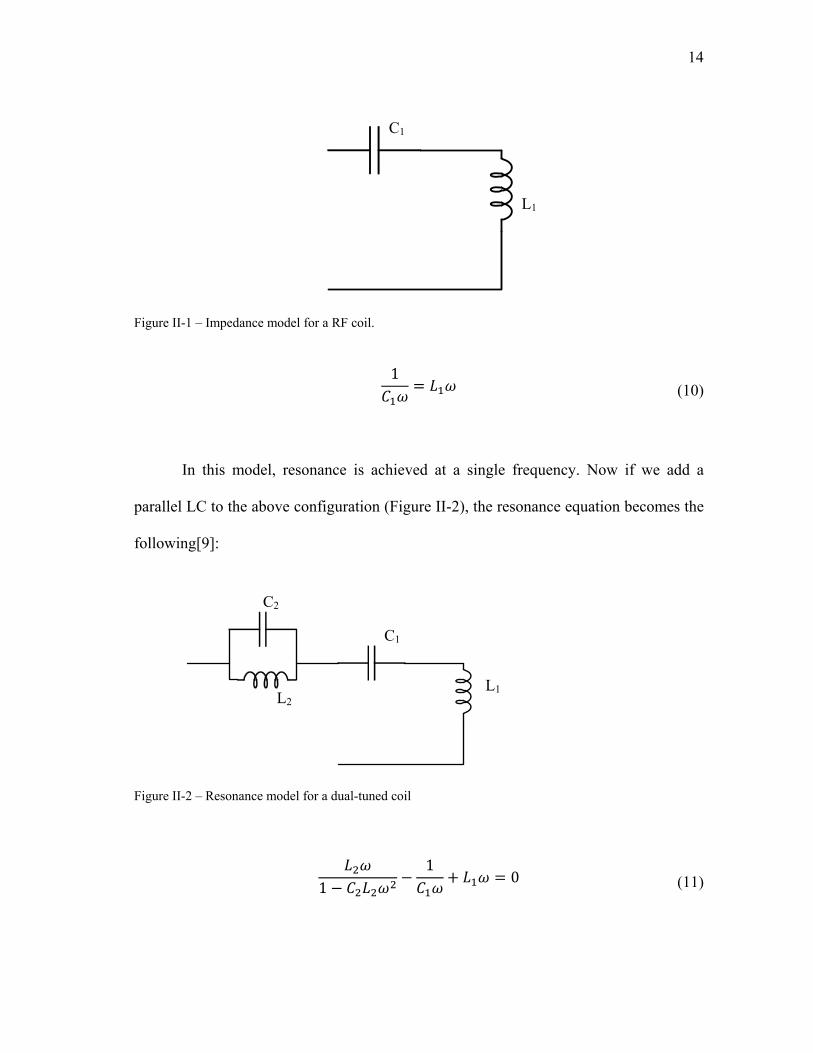
resonant elements[8]. Normally, in single-tuned coils (Figure II-1), a capacitor is used in
series12 with coil inductance to cancel-out the reactive impedance (series model is
normally used [9] to study dual-tuned resonance behavior and SNR)
1A series LC circuit resonates (zero impedance) at the same frequency as it would as a parallel resonator (infinite impedance). Matching/tuning strategy is merely a matter of transmission line characteristic impedance or the impedance required to noise-match a preamplifier and does not affect coil SNR and resonance frequency.
14
Figure II-1 – Impedance model for a RF coil.
1
(10)
In this model, resonance is achieved at a single frequency. Now if we add a
parallel LC to the above configuration (Figure II-2), the resonance equation becomes the
following[9]:
Figure II-2 – Resonance model for a dual-tuned coil
11
0 (11)
L2
C2
C1
L1
L1
C1

15
Or
1
1
11 0 (12)
where is the resonant frequency of the single-tuned coil and is the resonance
frequency of the trap.
There will be two frequencies (two modes) that satisfy the above equation and
can be used to operate the coil at minimum impedance required for effective
transmission and reception. Figure II-3 shows the reactance of a single-tuned coil
(dashed line) along with a parallel LC trap, generated using equation (12). Putting the
two in series will introduce two new resonant modes, corresponding to the intersections
of two graphs. Note that the trap has positive reactance at the lower frequency
(equivalent to an inductor) and negative reactance at the higher frequency (equivalent to
a capacitor). The lower mode will be close to the single-tuned coil resonance (thus
mostly governed by C1), and the higher mode will be close to the trap resonance (thus
mostly governed by C2 and L2).
At the higher-frequency mode, the current in the trap inductance is out-of-phase
with the current in the coil inductance; while at the lower-frequency mode, the current in
both inductors are in-phase.

16
Figure II-3 – Reactance of a single-tuned coil and a trap. The two intersections mark the two resonant modes of the trap in series with the coil.
The efficiency of this coil at the two frequencies might not be equal. Defining the
efficiency as the ratio of the power delivered to the load to the power dissipated in the
trap, it is shown[8] that at the higher frequency:
/
(13)
while at the lower frequency:
0
Frequency
trap reactance-(single-tuned reactance)
fL
fH
ω1ω2

17
/
(14)
At the higher frequency, we are operating close to the resonance mode of the trap circuit;
so a large trap inductance causes a higher circulating current in the tank circuit, and
higher noise contribution. So in order to minimize the effective trap loss at the higher
frequency, trap inductance needs to be chosen to be relatively higher than coil
inductance; while at the lower frequency (which is usually more critical because of low-
abundance nuclei) we are operating far lower than the trap resonance, so the current
running in the trap inductance L2 is approximately equal to the current running in the
coil inductance L1; so the effective trap loss will be proportional to the trap inductance
(assuming a fixed inductor Q). So it is necessary to choose L2 to be small compared to
L1. This tends to be one of the main disadvantages of the single-coil design, since a
major compromise needs to be made: if the design is optimized for the lower-frequency
nuclei, proton performance will be typically reduced by half [8].
In order to use this coil, impedance needs to be matched to 50 ohms. Dual-tuned
coils can have either a single input, where both modes are excited through a single port,
or two inputs. In sequential applications where simultaneous operation of the two modes
is not required, a single input coil can be used, along with a single-channel RF amplifier.
However in applications where two modes are operated at the same time (such as proton
decoupling), two separate inputs to the coil are required.
18
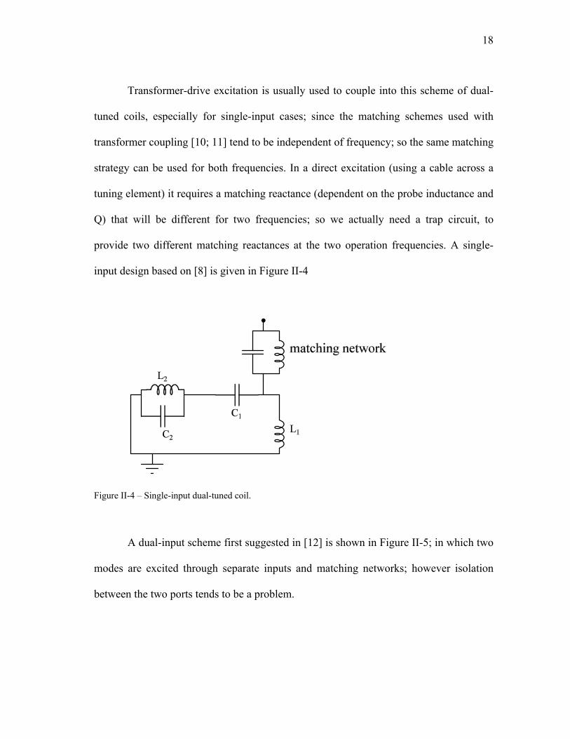
Transformer-drive excitation is usually used to couple into this scheme of dual-
tuned coils, especially for single-input cases; since the matching schemes used with
transformer coupling [10; 11] tend to be independent of frequency; so the same matching
strategy can be used for both frequencies. In a direct excitation (using a cable across a
tuning element) it requires a matching reactance (dependent on the probe inductance and
Q) that will be different for two frequencies; so we actually need a trap circuit, to
provide two different matching reactances at the two operation frequencies. A single-
input design based on [8] is given in Figure II-4
Figure II-4 – Single-input dual-tuned coil.
A dual-input scheme first suggested in [12] is shown in Figure II-5; in which two
modes are excited through separate inputs and matching networks; however isolation
between the two ports tends to be a problem.
19
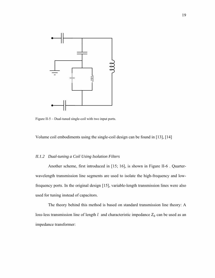
Figure II-5 – Dual-tuned single-coil with two input ports.
Volume coil embodiments using the single-coil design can be found in [13], [14]
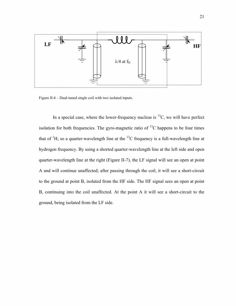
II.1.2 Dual-tuning a Coil Using Isolation Filters
Another scheme, first introduced in [15; 16], is shown in Figure II-6 . Quarter-
wavelength transmission line segments are used to isolate the high-frequency and low-
frequency ports. In the original design [15], variable-length transmission lines were also
used for tuning instead of capacitors.
The theory behind this method is based on standard transmission line theory: A
loss-less transmission line of length and characteristic impedance can be used as an
impedance transformer:
20
coscos (15)
where is the propagation constant equal to 2 / . With /4:
4 (16)
Therefore, An open-circuited quarter-wavelength ( ∞) will look like a short circuit,
and a short-circuited quarter-wavelength will look like an open circuit.
In Figure II-6, it can be seen that at the high frequency, the open-circuited line
on the left will look like a short circuit, blocking the high-frequency signal from getting
into the low-frequency part; while the short-circuited line on the right will look like an
open circuit, leaving the high-frequency signal unaffected.
The reason that line segments are designed at the high-frequency nuclei is that in
proton decoupling, the proton coil (high frequency) is transmitting large amounts of
power into the coil while the observation nuclei(low-frequency circuit) is receiving; so it
is crucial to isolate the high-power proton signal from low-frequency circuitry and
preamplifiers.
21
Figure II-6 – Dual-tuned single coil with two isolated inputs.
In a special case, where the lower-frequency nucleus is 13C, we will have perfect
isolation for both frequencies. The gyro-magnetic ratio of 13C happens to be four times
that of 1H; so a quarter-wavelength line at the 13C frequency is a full-wavelength line at
hydrogen frequency. By using a shorted quarter-wavelength line at the left side and open
quarter-wavelength line at the right (Figure II-7), the LF signal will see an open at point
A and will continue unaffected; after passing through the coil, it will see a short-circuit
to the ground at point B, isolated from the HF side. The HF signal sees an open at point
B, continuing into the coil unaffected. At the point A it will see a short-circuit to the
ground, being isolated from the LF side.
λ/4 at fH
HFLF

22
Lumped-element equivalents are suggested in [17] for an isolating filter which is
open at a desired frequency and short at a second one, generalizing this perfect isolation
to other nuclei pairs. The circuit in Figure II-8 (a), can act as an open at the higher
frequency and as a short at the lower frequency, so it is suitable for the HF side of the
dual-tuned coil (such as hydrogen). The design formulas are[17]:
1 (17)
1
(18)
A B HFLF
λ/4 at fL
Figure II-7 - Dual-tuned single coil for 13C and 1H.
23
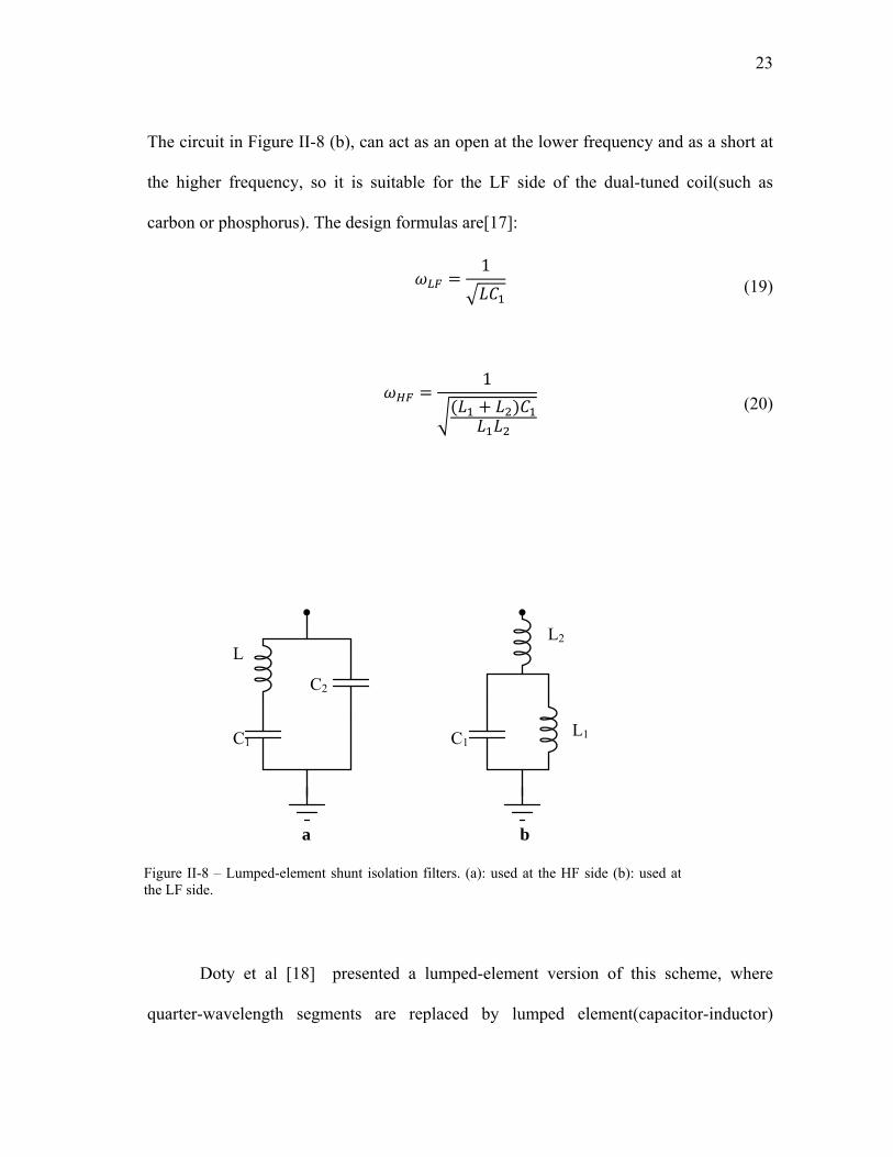
The circuit in Figure II-8 (b), can act as an open at the lower frequency and as a short at
the higher frequency, so it is suitable for the LF side of the dual-tuned coil(such as
carbon or phosphorus). The design formulas are[17]:
1 (19)
1 (20)
Doty et al [18] presented a lumped-element version of this scheme, where
quarter-wavelength segments are replaced by lumped element(capacitor-inductor)
L
C1
C2
L2
L1 C1
a b
Figure II-8 – Lumped-element shunt isolation filters. (a): used at the HF side (b): used atthe LF side.
24
equivalents for better efficiency. It is shown that by changing the ratio of the coil
inductor to the filter inductor, one can adjust the efficiency of the system and reach the
desired compromise between LF and HF efficiency, as well as a wide tuning range for
each.
II.2. Dual Coil Approach
While dual-tuned single coils(described in the previous section) have been used
in the past (especially in chemistry, where coils are small compared to the wavelength),
it is usually more advantageous to separate the two modes into two coils. With this
approach, each coil can be individually optimized for the application, and isolation
between the two is easier to achieve. Also, if using a phosphorus coil with existing
proton coils is desired, a two-coil design is obviously the method of choice.
Whenever two coils are placed in proximity of each other, the magnetic flux
generated by one is linked to the other coil(unless they are orthogonal to each other).
Using Faraday’s induction law for a RF magnetic field linked to a coil of surface Σ :
· (21)
This EMF produces an induced current on the second coil, which can be modeled
as a circuit with mutual inductance (Figure II-9).
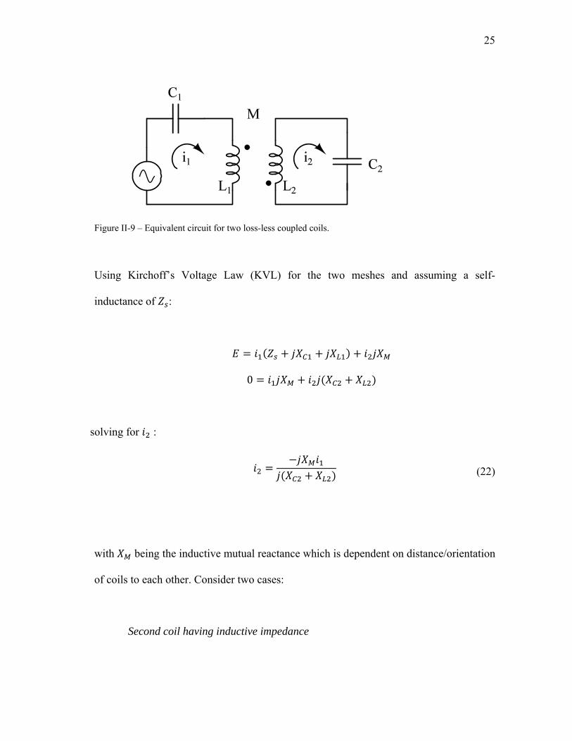
25
Figure II-9 – Equivalent circuit for two loss-less coupled coils.
Using Kirchoff’s Voltage Law (KVL) for the two meshes and assuming a self-
inductance of :
0
solving for :
(22)
with being the inductive mutual reactance which is dependent on distance/orientation
of coils to each other. Consider two cases:
Second coil having inductive impedance
26
In this case, will be positive, and using equation (22):
, i.e. current induced in the second coil will be 180 degrees out of phase
with the excitation current in the main coil.
Second coil having capacitive impedance
In this case, will be negative, and using equation (22): , i.e.
current induced in the second coil will be in phase with the excitation current in the main
coil.
A series LC resonator operated above its resonance frequency will have inductive
reactance; thus supporting an induced current counter-rotating from the excitation
current. Similarly, a resonator operated below its resonance frequency will have
capacitive reactance supporting an induced current co-rotating with the excitation
current.
Therefore, when we are operating the system at the hydrogen frequency, the
phosphorus coil will act as an inductor; while at the phosphorus frequency, hydrogen
coil will act as a capacitor. Fitzsimmons et al. [19; 20] showed this phenomenon by
PSpice™ simulation of current phase responses. Depending on orientation of the two
27
coils to each other, the counter-rotating currents can cause significant loss in magnetic
field intensity.
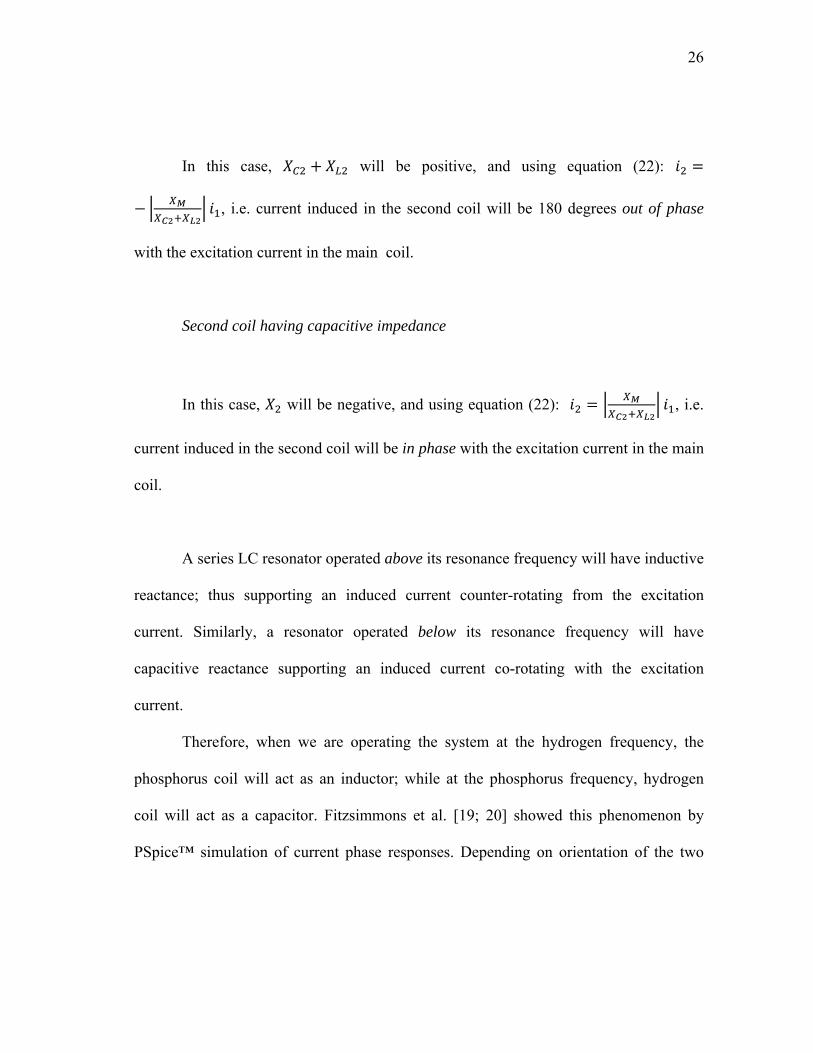
Geometric decoupling is one method used in the past to fix this problem of
counter-productive current generation. If we can produce a proton magnetic field
perfectly parallel to the phosphorus coil plane, there will be no flux linked with the
phosphorus coil, and there will be no induced currents. A figure-8 shaped, or butterfly
coil[21] (shown in Figure II-10-b) provides a magnetic field parallel to the coil plane (in
the middle), significantly reducing the coupling to the normal 31P field. Another design,
known as co-planar dual-loop surface coil[22], consists of a center-fed loop, producing
counter-rotating currents in the half-loops, which will create a magnetic field parallel to
the plane. (Figure II-10-a)
Although these designs provide good decoupling between the proton coil and
phosphorus coil, the parallel magnetic field intensity produced by the proton coil tends
to fall off very quickly as we move away from the coil plane; so if the region of interest
Figure II-10 – Two coil designs producing a magnetic field parallel to their plane. Current and magnetic field directions are shown. At the middle of the coil, magnetic field is parallel to the plane. (a) Butterfly or figure-8 coil design and (b) co-planar dual loop design.
a b

28
is located at deeper distances, this design will not provide sufficient proton performance.
A more recent design [23] is shown in Figure II-11. Two proton surface coils are
wrapped around a half-cylinder formation, to produce orthogonal magnetic field in the
center. Using the fact that the magnetization in the material is also circularly polarized,
this method provides a significant gain compared to a linearly-polarized magnetic field.
If the two coils are fed with a signal and its 90 degree phased-shifted version, it
will produce a RF magnetic field with circular polarization. Effective transverse coil
sensitivity is defined as:
· (23)
where √
. For a linearly-polarized coil:
, | | ·1
√21
√2| | (24)
If we use a 3 dB, 90 degree phase-shift power divider (known as a quadrature hybrid
combiner) to divide the power by 2 (divide the field magnitude by √2) and feed the in-
phase signal to one coil and quadrature-phase signal to the orthogonal coil, it will
produce a circularly-polarized field
, | |1
√21
√2·
1√2
| | (25)
which is equivalent to a sensitivity gain by a factor of √2 and transmitted power gain by
a factor of 2.

29
By placing the lower-frequency coil at a distance from the protons, the blocking
field problem is reportedly [23] solved (as shown in Figure II-11 ), providing -20 dB
isolation between the 31C coil and 1H coils. Isolation between two quadrature proton
coils is achieved by overlapping the two, providing a shared flux area that cancels out
the direct flux linkage between the two.
This chapter has reviewed the basic design options for dual-frequency NMR
excitation coils. An emphasis has been placed on dual-coil design methods, as this
provides a direct route towards developing “insertability” capabilities for second nuclei
coils. The following chapter presents the primary design consideration to enable this
insertability.
1H 1H 31P
1Hq 1HI
Figure II-11 – Half-volume quadrature dual-tuned coil design.

30
CHAPTER III
USING TRAPS IN DUAL-COIL DESIGN
Various design approaches to the dual-tuning problem were discussed in the
previous chapter. A particular design, using a trap circuit tuned to the 1H frequency on
the 31P coil was chosen, implemented, and thoroughly analyzed in this project, using
bench measurements as well as imaging/spectroscopy tests. An analytical model is
developed and guidelines on trap design are provided to help optimize performance.
The main advantage of this method is enabling the design of second-nuclei coils that are
insertable into standard proton coils, maintaining a near-optimum performance for both
nuclei.
III.1. Tank Circuits
LC traps are tank circuits composed of an inductor and capacitor in parallel,
providing very high impedance at the tank resonance frequency. The first example of
usage in NMR coils appears in [24], where a trap is used as an external filter, along the
dual-tuned receiver chain, in order to isolate the two frequencies in a dual-tuned TEM
(transverse electromagnetic) coil.
Ideal traps have no loss; and provide infinite impedance at their resonance.
Unfortunately inductors have a resistance associated with them(typical inductor Q is
below 300, while for capacitors it is usually above 1000); thus particularly limiting
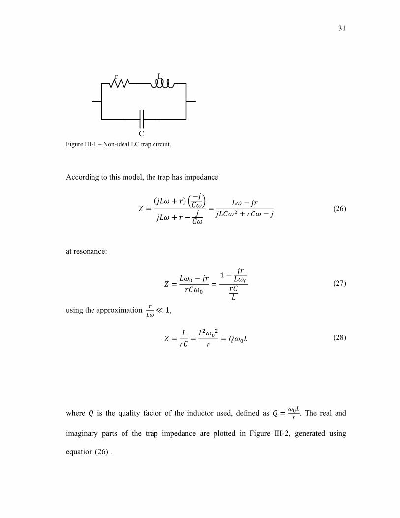
performance. A model of this non-ideal trap circuit is diagrammed in Figure III-1.
31
Figure III-1 – Non-ideal LC trap circuit.
According to this model, the trap has impedance
(26)
at resonance:
1 (27)
using the approximation 1,
(28)
where is the quality factor of the inductor used, defined as 0 . The real and
imaginary parts of the trap impedance are plotted in Figure III-2, generated using
equation (26) .
L r
C
32
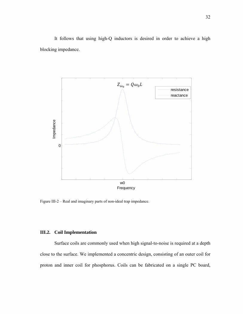
It follows that using high-Q inductors is desired in order to achieve a high
blocking impedance.
Figure III-2 – Real and imaginary parts of non-ideal trap impedance.
III.2. Coil Implementation
Surface coils are commonly used when high signal-to-noise is required at a depth
close to the surface. We implemented a concentric design, consisting of an outer coil for
proton and inner coil for phosphorus. Coils can be fabricated on a single PC board,
w0
0
Frequency
Impe
danc
e
resistancereactance

33
however we will show later that a modular, separable design is essential for optimization
of the trap as well as application flexibility (potential of having a stand-alone 31P coil,
insertable into proton coils). Two loops were cut(12.44 cm and 7.1 cm diameter, 1 cm
wide) from a FR-4 PCB (which is known to provide good Q) using in-house protoboard
machine (LPKF C30, Wilsonville, OR). In anticipation of high-field surface coil design,
a shield was included to limit radiation loss. The coil configuration is shown in Figure
III-3.
Figure III-3 – Concentric surface coil structure.
In a standard surface coil fashion, four equally spaced gaps were cut to place
tuning elements and ensure in-phase current at different locations along the loop, despite
the high operation frequency. Resonance was achieved by placing surface-mount
34
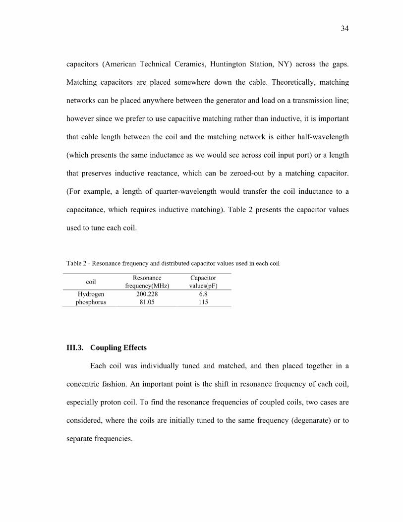
capacitors (American Technical Ceramics, Huntington Station, NY) across the gaps.
Matching capacitors are placed somewhere down the cable. Theoretically, matching
networks can be placed anywhere between the generator and load on a transmission line;
however since we prefer to use capacitive matching rather than inductive, it is important
that cable length between the coil and the matching network is either half-wavelength
(which presents the same inductance as we would see across coil input port) or a length
that preserves inductive reactance, which can be zeroed-out by a matching capacitor.
(For example, a length of quarter-wavelength would transfer the coil inductance to a
capacitance, which requires inductive matching). Table 2 presents the capacitor values
used to tune each coil.
Table 2 - Resonance frequency and distributed capacitor values used in each coil
coil Resonance frequency(MHz)
Capacitor values(pF)
Hydrogen 200.228 6.8 phosphorus 81.05 115
III.3. Coupling Effects
Each coil was individually tuned and matched, and then placed together in a
concentric fashion. An important point is the shift in resonance frequency of each coil,
especially proton coil. To find the resonance frequencies of coupled coils, two cases are
considered, where the coils are initially tuned to the same frequency (degenarate) or to
separate frequencies.
35
III.3.1 Initially Tuned Degenerate
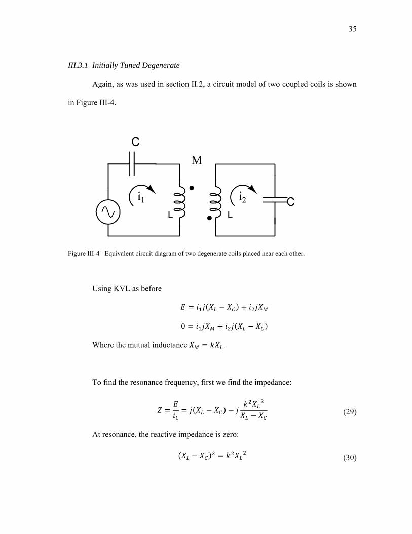
Again, as was used in section II.2, a circuit model of two coupled coils is shown
in Figure III-4.
Figure III-4 –Equivalent circuit diagram of two degenerate coils placed near each other.
Using KVL as before
0
Where the mutual inductance .
To find the resonance frequency, first we find the impedance:
(29)
At resonance, the reactive impedance is zero:
(30)

36
After expansion and division by :
1 2 1 (31)
Knowing that coils are individually tuned to :
Substituting into (31):
1 2 1 0
1 1 11
11 (32)
Knowing that 1 , it is shown that coupling causes the resonance frequency to
split apart into two frequencies.
III.3.2 Initially Tuned to Separate Frequencies
This is the case with multi-nuclear coils; since each one is tuned to the nucleus
of interest. Equation (30) becomes
After expansion and division by :
37
1 1 · (33)
Knowing the fact that coil 1 is tuned to and coil 2 is tuned to :
,
Substituting into (33) :
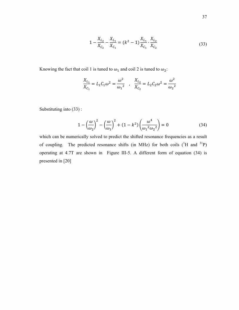
1 1 0 (34)
which can be numerically solved to predict the shifted resonance frequencies as a result
of coupling. The predicted resonance shifts (in MHz) for both coils (1H and 31P)
operating at 4.7T are shown in Figure III-5. A different form of equation (34) is
presented in [20]

38
Figure III-5 – Effect of coil coupling between 1H coil and 31P coil at 4.7T, manifesting itself as a shift in the desired resonance frequency.
III.4. Bench Measurement Results
In case of our concentric coils, coupling caused the proton resonance frequency
to move up to 208 MHz and phosphorus resonance frequency down to 80.05MHz.
Figure III-6 depicts a screenshot from Agilent 5071 network analyzer showing this
resonant shift.
0 0.1 0.2 0.3 0.4 0.5 0.6 0.7 0.8
81.05100
150
200.23
250
300
350
Coupling Constant k
Res
onan
ce F
requ
ency
(MH
z)
Proton Mode
Phosphorus Mode
39
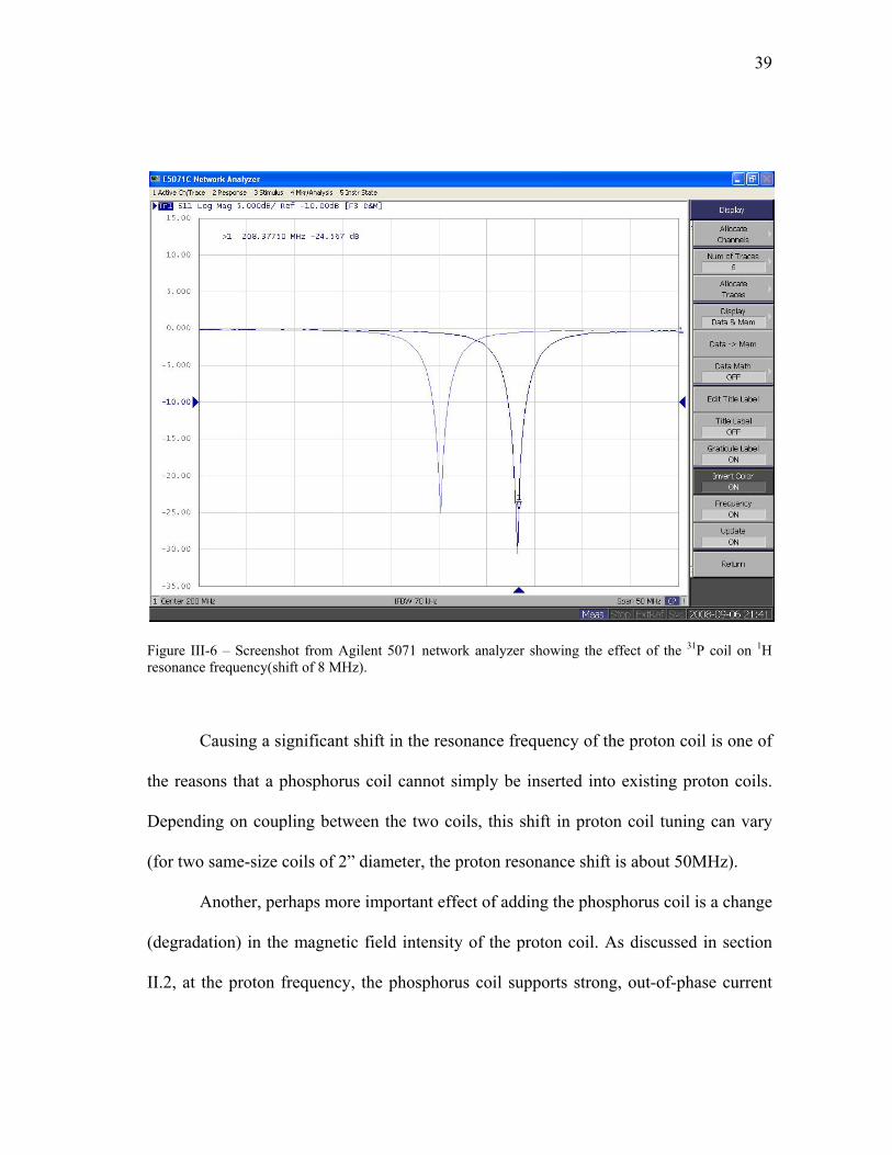
Figure III-6 – Screenshot from Agilent 5071 network analyzer showing the effect of the 31P coil on 1H resonance frequency(shift of 8 MHz).
Causing a significant shift in the resonance frequency of the proton coil is one of
the reasons that a phosphorus coil cannot simply be inserted into existing proton coils.
Depending on coupling between the two coils, this shift in proton coil tuning can vary
(for two same-size coils of 2” diameter, the proton resonance shift is about 50MHz).
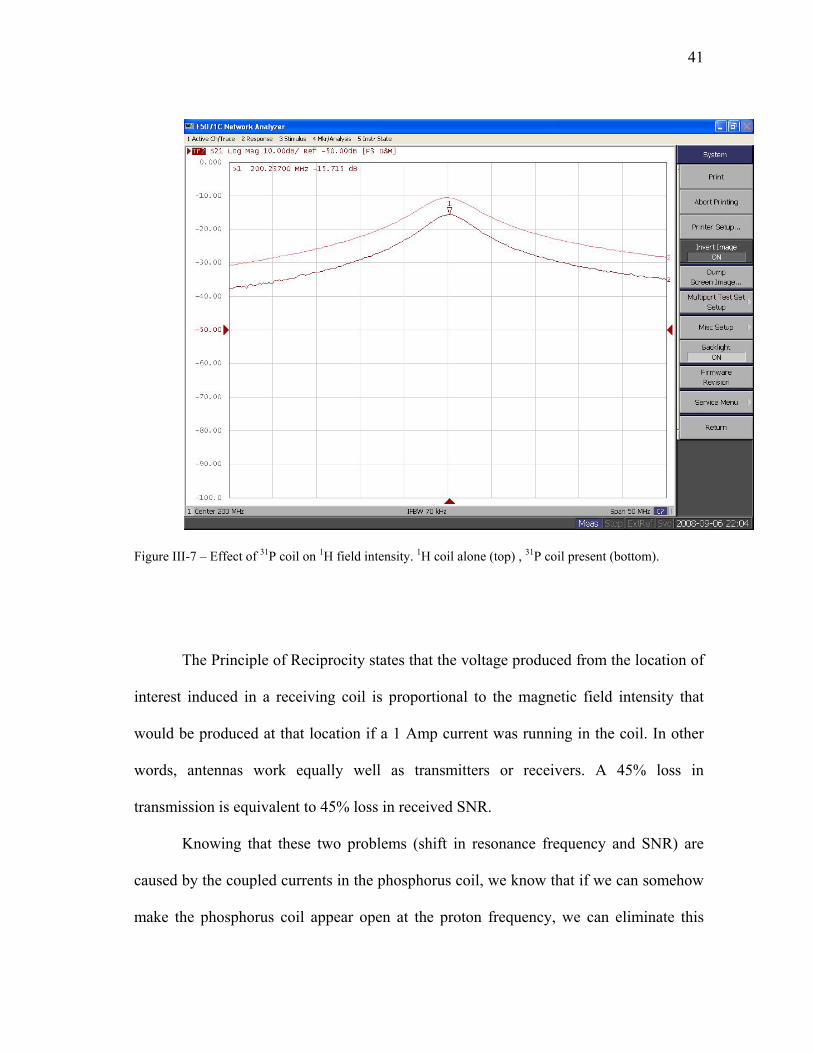
Another, perhaps more important effect of adding the phosphorus coil is a change
(degradation) in the magnetic field intensity of the proton coil. As discussed in section
II.2, at the proton frequency, the phosphorus coil supports strong, out-of-phase current

40
that effectively blocks the magnetic field produced by the proton coil in the center. This
effect is shown in Figure III-7. The standard method to estimate field intensity and SNR
of a coil is to excite a matched coil using a cable and receive the signal by a field probe
(known as “pick-up loop”). Using a network analyzer, this can be done using an S21
measurement. It is important to maintain the tune/match when using this method to
compare different coils. One can also use a loop (dual pick-up loop consists of two
decoupled small loops, one for excitation and one for detection. It is also used to find
resonance frequency and Q of a resonator) in order to inductively excite the coil instead
of using a 50 ohm cable; making the measurement less prone to change in matching
conditions. In Figure III-7, the magnetic field is measured on the axis, at 2.5 cm (1/3 coil
width) above the coil surface. The top curve is for the proton coil alone, and the bottom
curve is after putting on the phosphorus coil and retuning/rematching. 4.7 dB loss in the
on-axis magnetic field intensity is observed, corresponding to about 45% loss in
magnetic field intensity generated by the proton coil.
41
Figure III-7 – Effect of 31P coil on 1H field intensity. 1H coil alone (top) , 31P coil present (bottom).
The Principle of Reciprocity states that the voltage produced from the location of
interest induced in a receiving coil is proportional to the magnetic field intensity that
would be produced at that location if a 1 Amp current was running in the coil. In other
words, antennas work equally well as transmitters or receivers. A 45% loss in
transmission is equivalent to 45% loss in received SNR.
Knowing that these two problems (shift in resonance frequency and SNR) are
caused by the coupled currents in the phosphorus coil, we know that if we can somehow
make the phosphorus coil appear open at the proton frequency, we can eliminate this
42
current. Alecci et al[25] used LC traps, tuned to proton frequency, on their Na coil. In
order to tune this trap properly, one can start with designed values; however the
capacitor is usually chosen variable to make fine-tuning easier. Once the right
capacitance was found, it can be switched with a fixed capacitor. The first step is to tune
and match the proton coil to the right frequency (200.228MHz). Then, the phosphorus
coil is placed in the center, and the variable capacitor of the trap is tuned, such that
proton coil resonance (S11 or S21 as measured by a pick-up loop) goes back to where it
was before adding the phosphorus coil; i.e. phosphorus coil should be invisible to the
proton coil, at the proton frequency. Having two coils present from the beginning and
tuning the trap to get the desired resonance frequency will be incorrect; since the
obtained tuning might be a result of unresolved coupling. It is notable that this process of
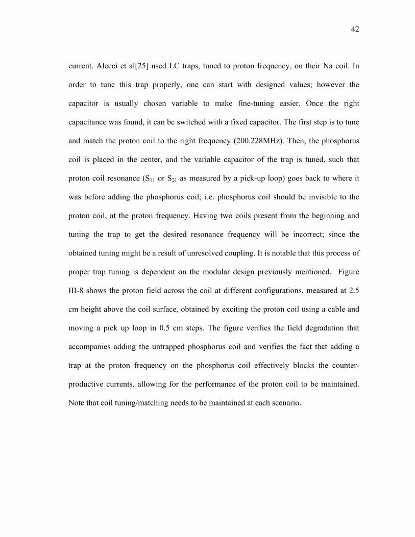
proper trap tuning is dependent on the modular design previously mentioned. Figure
III-8 shows the proton field across the coil at different configurations, measured at 2.5
cm height above the coil surface, obtained by exciting the proton coil using a cable and
moving a pick up loop in 0.5 cm steps. The figure verifies the field degradation that
accompanies adding the untrapped phosphorus coil and verifies the fact that adding a
trap at the proton frequency on the phosphorus coil effectively blocks the counter-
productive currents, allowing for the performance of the proton coil to be maintained.
Note that coil tuning/matching needs to be maintained at each scenario.
43
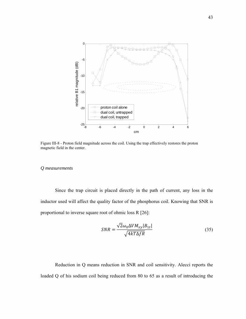
Figure III-8 - Proton field magnitude across the coil. Using the trap effectively restores the proton magnetic field in the center.
Q measurements
Since the trap circuit is placed directly in the path of current, any loss in the
inductor used will affect the quality factor of the phosphorus coil. Knowing that SNR is
proportional to inverse square root of ohmic loss R [26]:
√2 ∆ | |
4 ∆ (35)
Reduction in Q means reduction in SNR and coil sensitivity. Alecci reports the
loaded Q of his sodium coil being reduced from 80 to 65 as a result of introducing the
-8 -6 -4 -2 0 2 4 6-25
-20
-15
-10
-5
0
cm
rela
tive
B1
mag
nitu
de (d
B)
proton coil alonedual coil, untrappeddual coil, trapped

44
trap (implying a proportional loss in SNR). Capacitors are high-Q components, so the
inductor used in the trap is indeed the Q bottleneck.We used an air-core, six turn 22nH
inductor (Coilcraft, Cary, IL) which provides a high Q ( datasheet specifications are
shown in Figure III-9).
Figure III-9 – Q factor of the inductor (22nH) used to make the trap. Courtesy of Coilcraft, Inc.
To measure the Q of the coil, the cables were removed (since cable loss would be
fixed in either case, and to eliminate any radiation losses) and dual pick-up loops were
used at about 2cm above the coil. The unloaded to loaded Q was measured as 105/60,
and it did not change after introducing the trap. This means the trap loss is negligible
compared to the coil/sample loss in this case. We believe that this is due primarily to the

45
use of high-quality components. No change in loaded Q ensures that there will be no
SNR drop due to trap circuit losses.
III.5. SNR Model
III.5.1 B1 Magnitude
Again considering two coupled loops (Figure III-10), with the first one tuned to
1H and the second one tuned to 31P, the induced current in the phosphorus coil can be
calculated as:
Figure III-10 – Coupled dual-tuned resonators.

46
1 (36)
(37)
with being the resonance frequency of the second loop, i.e. phosphorus in our case, in
absence of coupling (81.45 MHz at 4.7T). As previously discussed, considering the
higher frequency mode (proton), will be negative, indicating an induced
current at -180 degrees from the excitation current, which will oppose the proton
magnetic field. The total magnetic field at the distance on the axis will thus be [27]
. 2 / . / (38)
according to Biot-Savart, where = radius of the 1H (outer) coil and = radius of the
31P (inner) coil.
The mutual inductance between two circular loops can be approximated as [28]
√2
1 2 ,4
(39)

47
where and are complete elliptic integrals of the first and second kind
(respectively), and is equal to distance between two planes, which is zero in co-planar
design. By measuring the L2=155nH, we can plot the total magnetic field intensity on the
axis (Figure III-11).
Figure III-11 - Effect of 31P coupling in 1H coil field strength along the axis. Coil diameters are 7.1 cm for 31P and 12.44cm for 1H.
0 1 2 3 4 5 6 7 8 9 101
2
3
4
5
6
7
8
9
10
11x 10-6
cm
Tesl
a/A
mp
proton coil alonephosphorus coil present

48
In order to model the trap effect on the proton B1 magnitude, we can find the
effective impedance of a non-ideal trap using equation (28), which is dependent on the
frequency, the quality factor (Q), and inductor value (L). Using a low-Q inductor
reduces the effective trap impedance. Considering a fixed Q (Figure III-9), the trap
impedance will be proportional to the inductor value (however this will introduce loss in
the 31P coil; see Section III.5.2). To model the Q effect on blocking effectiveness of the
trap, we can modify the equivalent circuit used earlier to include the trap impedance
(Figure III-12).
Figure III-12 – Coupled dual-tuned resonators with a trap included.
The current ratio will then be
where .
Total magnetic field magnitude on the axis will then be
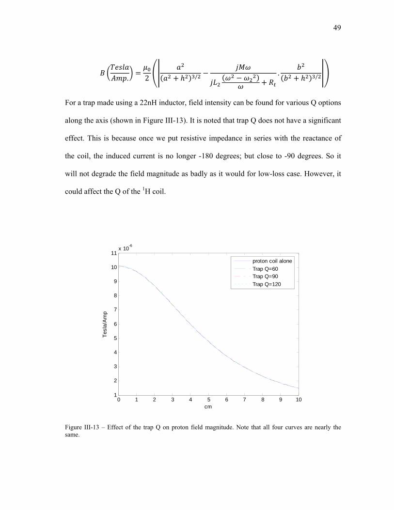
49
. 2 / . /
For a trap made using a 22nH inductor, field intensity can be found for various Q options
along the axis (shown in Figure III-13). It is noted that trap Q does not have a significant
effect. This is because once we put resistive impedance in series with the reactance of
the coil, the induced current is no longer -180 degrees; but close to -90 degrees. So it
will not degrade the field magnitude as badly as it would for low-loss case. However, it
could affect the Q of the 1H coil.
Figure III-13 – Effect of the trap Q on proton field magnitude. Note that all four curves are nearly the same.
0 1 2 3 4 5 6 7 8 9 101
2
3
4
5
6
7
8
9
10
11x 10-6
cm
Tesl
a/A
mp
proton coil aloneTrap Q=60Trap Q=90Trap Q=120

50
III.5.2 Noise Level
Inductors are usually considered to be lossy elements. Adding lossy elements to
the coil resonator introduces thermal noise, which degrades coil sensitivity or SNR.
Considering the per unit current to be equal in both cases, sensitivity ratio, defined as
SNR of the untrapped coil divided by SNR of the trapped coil, will be
1
1 (40)
where is the resistance of the coil conductor and is the effective trap resistance
being added to the system.
At the 31P frequency, using equation (26), the effective trap resistance
appearing in series with the coil resistance will be equal to the actual trap inductor
resistance (with a very good approximation; since the trap is far away from resonance).
Equation (40) becomes
1
· 1 (41)
where is the inductor value used in the trap, is the Q of the trap, is the 31P coil
inductance, and is the loaded 31P coil Q, before introduction of the trap.
51
At the 1H frequency, using equation (29) to transform the resonant trap resistance
to the proton side of the circuit, effective trap resistance can be found as:
(42)
where is the mutual reactance at 1H frequency, and is the reactance of the 31P coil
at 1H frequency. Assuming :
(43)
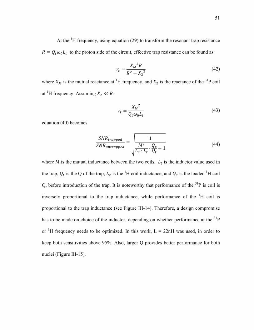
equation (40) becomes
1
· · 1 (44)
where is the mutual inductance between the two coils, is the inductor value used in
the trap, is the Q of the trap, is the 1H coil inductance, and is the loaded 1H coil
Q, before introduction of the trap. It is noteworthy that performance of the 31P is coil is
inversely proportional to the trap inductance, while performance of the 1H coil is
proportional to the trap inductance (see Figure III-14). Therefore, a design compromise
has to be made on choice of the inductor, depending on whether performance at the 31P
or 1H frequency needs to be optimized. In this work, L = 22nH was used, in order to
keep both sensitivities above 95%. Also, larger Q provides better performance for both
nuclei (Figure III-15).

52
Figure III-14 – Effect of the trap inductor value on coil performance. A quality factor Q=150 is assumed.
10 15 20 25 30 35 40 450.89
0.9
0.91
0.92
0.93
0.94
0.95
0.96
0.97
0.98
0.99
trap inductor value (nH)
trapp
ed S
NR
/unt
rapp
ed S
NR
proton coilphosphorus coil
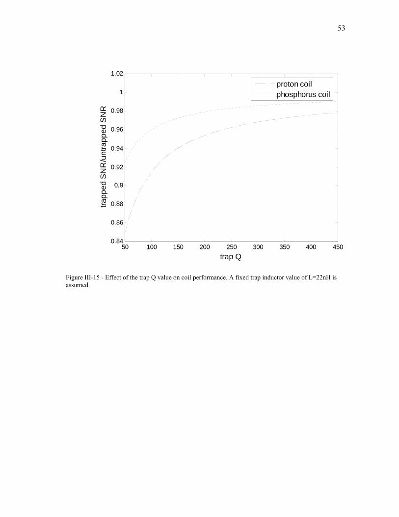
53
Figure III-15 - Effect of the trap Q value on coil performance. A fixed trap inductor value of L=22nH is assumed.
50 100 150 200 250 300 350 400 4500.84
0.86
0.88
0.9
0.92
0.94
0.96
0.98
1
1.02
trap Q
trapp
ed S
NR
/unt
rapp
ed S
NR
proton coilphosphorus coil

54
CHAPTER IV
MRI/MRS TESTING
In this chapter, we examine use of MR images and spectra as indices for coil
performance, and discuss the methodology of performing spectroscopy on the laboratory
Varian Inova system
IV.1. Spectroscopy Using the Varian Inova System
A 4.7 Tesla, 33 cm Varian Inova MR system located in the Magnetic Resonance
Lab at Texas A&M University was used for all data acquisition.
IV.1.1 System Modifications
Pulsed spectroscopy is performed in a similar fashion to imaging; however
certain system modifications need to be done. There are certain hardware components
(besides the RF coil, obviously) that are frequency-selective; for example, to operate the
same coil in both transmit and receive mode, a T/R switch is used, containing a quarter-
wavelength transmission line segment, keeping the transmit power from getting into
receive circuitry. For each nucleus being interrogated, the quarter-wavelength needs to
be adjusted based on the Larmor frequency of that nucleus. For example, the 25 cm RG-
58 cable normally used for 1H (200MHz at 4.7T) needs to be switched with a 62 cm one
for 31P(81.05MHz at 4.7 T). The 200MHz balun in line to the transceiver needs to be
bypassed. Also, a bandpass filter is used at the input to the RF amplifier to minimize

55
unwanted tones. Normally a Mini-Circuits (Brooklyn, NY) low-pass 0-200 MHz filter is
used for proton; it was switched with a SIF-70 bandpass filter for phosphorus.
IV.1.2 Shimming
Inhomogeneity in B0 results in added frequency components in the received free-
induction-decay (FID) signal. When imaging, those shifts are usually powered by the
gradients, however in spectroscopy, small shifts will show up next to the main peak,
broadening its line, reducing the peak value (since the signal is divided over a range of
frequencies) and hiding spectral information. Therefore proper shimming of the static B
field is essential prior to spectroscopy.
For in-vivo experiments on brain and liver tissues, shimming to less than 0.1 ppm
is required[29]; however for phantom studies where chemical shifts are several ppms
apart, about 1 ppm resolution is sufficient. Since the signal intensity acquired from
phosphorus atoms is much weaker than hydrogen, one can do the shimming on water
first (using the 1H coil), and then switch the coils without moving the phantom. This is
indeed one of the benefits of having a dual-tuned coil with two inputs. In our
experiments, shimming was accomplished to less than 50 Hz FWHM (see Figure IV-1).

56
Figure IV-1 – 1H spectra obtained to measure linewidth after shimming. For acquiring phosphorus spectra, the linewidth was shimmed to less than 50Hz (0.62ppm).
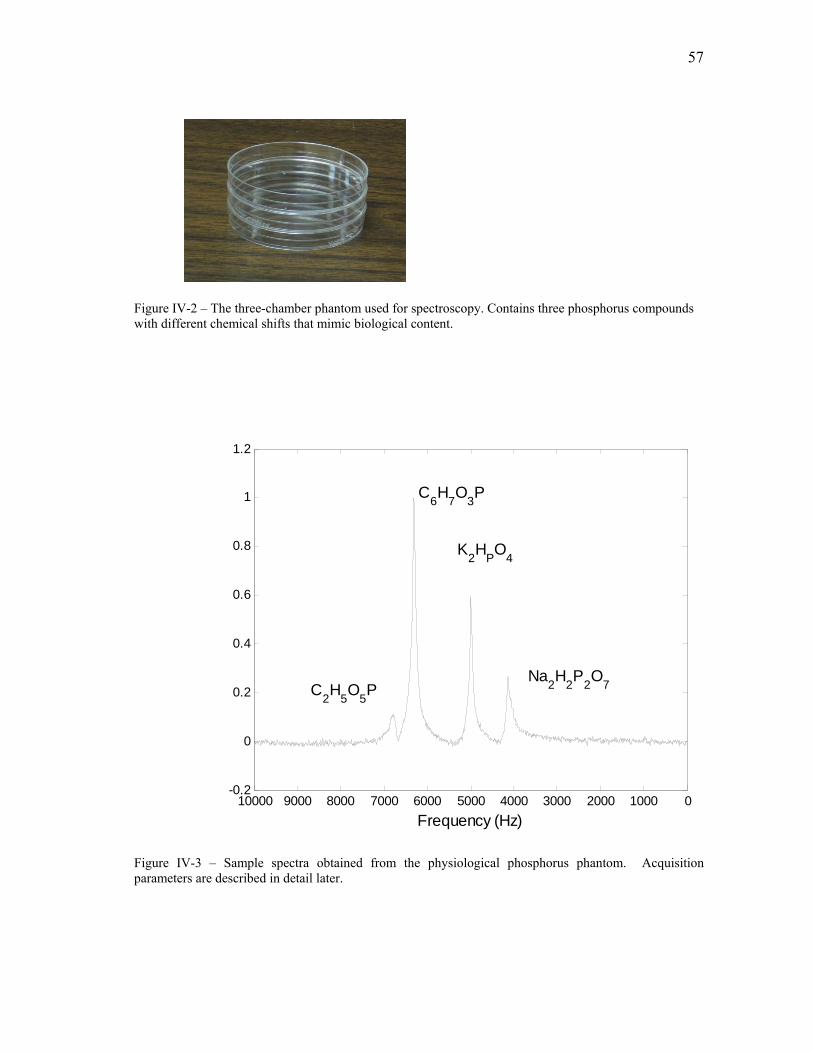
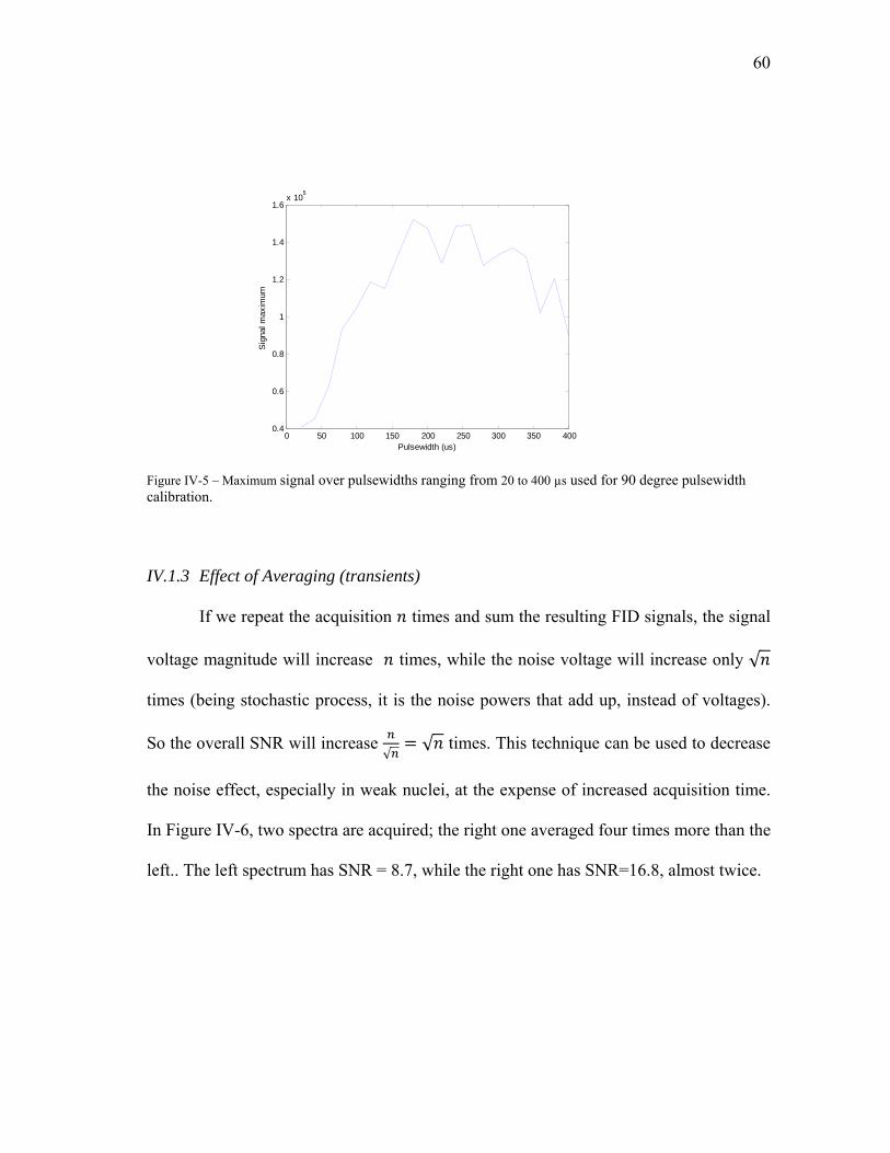
A phantom composed of three isolated chambers containing three phosphorus
compounds with different chemical shifts, mimicking those of common biological
phosphorus content [30], was used to acquire test spectra (Figure IV-2). Each chamber is
58 mm wide and 8 mm deep. From bottom to top, the chambers contain 1 M phenyl
phosphonic acid (C6H7O3P), 0.5M potassium phosphate (K2HPO4), 0.5M disodium
pyrophosphate (Na2H2P2O7). A test tube containing 1.5M phosphoacetic acid (C2H5O5P)
was also placed underneath the coil. (It is sometimes used for in vivo studies as a
chemical shift reference, in a small capillary). Figure IV-3 shows sample spectra
obtained for 10 kHz spectral width. Other parameters will be described in detail later.
0 1000 2000 3000 4000 5000 6000 7000 8000 9000 100000
1
2
3
4
5
6
7
8
9x 10⁶
Hz
57
Figure IV-2 – The three-chamber phantom used for spectroscopy. Contains three phosphorus compounds with different chemical shifts that mimic biological content.
Figure IV-3 – Sample spectra obtained from the physiological phosphorus phantom. Acquisition parameters are described in detail later.
010002000300040005000600070008000900010000-0.2
0
0.2
0.4
0.6
0.8
1
1.2
Frequency (Hz)
C2H5O5P
K2HPO4
C6H7O3P
Na2H2P2O7

58
Effects of pulse width/power
Among the parameters that need to be set are the duration of the pulsewidth and
transmitted power required to obtain a 90 tip angle. During application of a RF pulse, the
rotational frequency of the net magnetization vector is given by
Ω (45)
where is the effective field for the polarization being used. The tipped angle
following seconds of radiation is given by
(46)
which is proportional to pulse power and duration. In our experiment (using a typical
spin echo sequence), since the surface coil field has different field sensitivity at different
heights, some chambers might be under-tipped or over-tipped. Adiabatic plane-rotation
pulse sequences such as BIR-4 [31] can be used to get homogeneous field at different
heights, providing 90 degree tip for the entire sensitive volume of the surface coil.
However, using regular rectangular pulses, different peaks on the spectra obtained from
an inhomogeneous phantom will be affected by B1 magnitude at that chamber. In Figure
IV-4 (a), the first chamber has the tallest peak (closest tip angle to 90), however by
doubling the pulsewidth, the second chamber yields the maximum signal, while the first

59
one over-tips, reducing signal strength during readout. In our acquisitions, pulsewidth
was optimized for the first chamber.
One can calibrate the pulsewidth to get maximum signal. To do so, first we
needed to narrow the spectral width down to a single peak (first chamber; second peak
from the left). Then, set an array of pulsewidths ranging from 20 to 400 µs, and then
manually compared the array of signals. Figure IV-5 shows the maximum signal
occurring at about 200 µs.
Figure IV-4 – Effect of power on spectra obtained from an inhomogeneous phantom. (a): pulsewidth optimized for the first chamber. (b): pulsewidth optimized for the second chamber.
a b 0 500 1000 1500 2000 2500 3000 3500 4000 4500
0
0.5
1
1.5
2
2.5
3
3.5x 10
6
0 500 1000 1500 2000 2500 3000 3500 4000 45000
0.5
1
1.5
2
2.5
3
3.5x 10
6
60
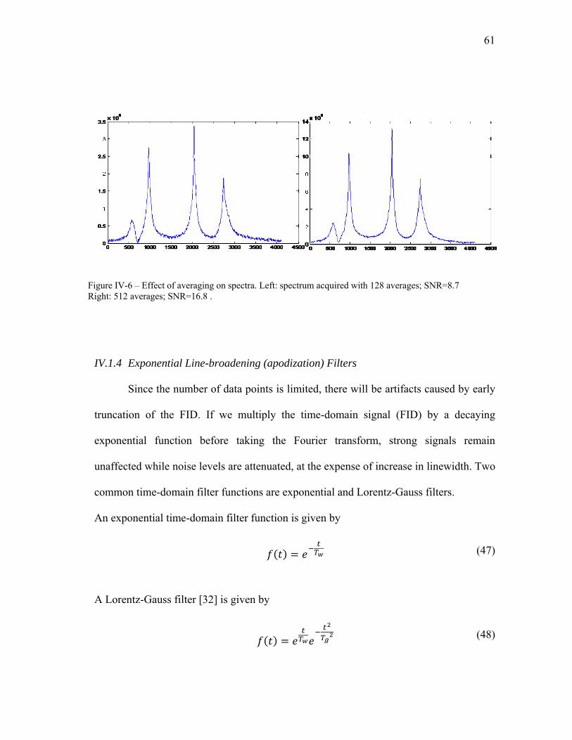
IV.1.3 Effect of Averaging (transients)
If we repeat the acquisition times and sum the resulting FID signals, the signal
voltage magnitude will increase times, while the noise voltage will increase only √
times (being stochastic process, it is the noise powers that add up, instead of voltages).
So the overall SNR will increase √
√ times. This technique can be used to decrease
the noise effect, especially in weak nuclei, at the expense of increased acquisition time.
In Figure IV-6, two spectra are acquired; the right one averaged four times more than the
left.. The left spectrum has SNR = 8.7, while the right one has SNR=16.8, almost twice.
Figure IV-5 – Maximum signal over pulsewidths ranging from 20 to 400 µs used for 90 degree pulsewidth calibration.
0 50 100 150 200 250 300 350 4000.4
0.6
0.8
1
1.2
1.4
1.6x 10⁵
Pulsewidth (us)
Sig
nal m
axim
um
61
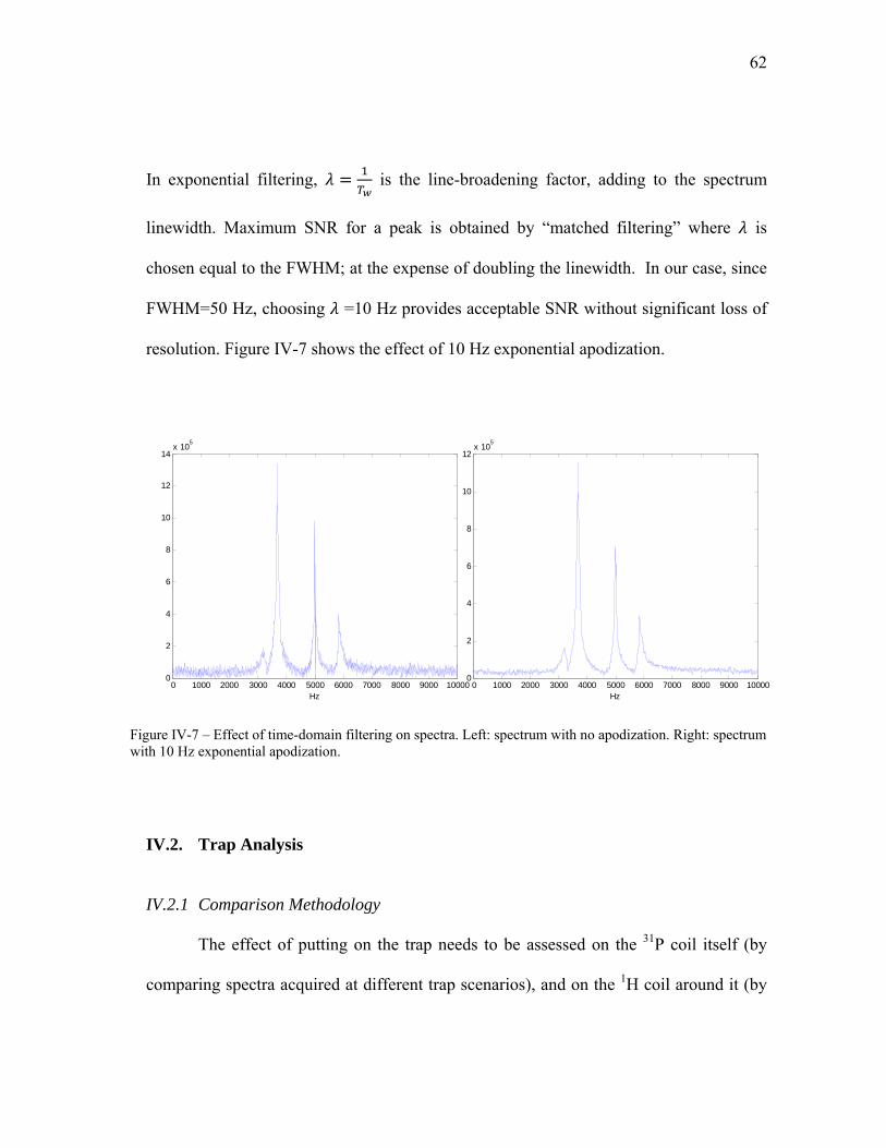
IV.1.4 Exponential Line-broadening (apodization) Filters
Since the number of data points is limited, there will be artifacts caused by early
truncation of the FID. If we multiply the time-domain signal (FID) by a decaying
exponential function before taking the Fourier transform, strong signals remain
unaffected while noise levels are attenuated, at the expense of increase in linewidth. Two
common time-domain filter functions are exponential and Lorentz-Gauss filters.
An exponential time-domain filter function is given by
(47)
A Lorentz-Gauss filter [32] is given by
(48)
Figure IV-6 – Effect of averaging on spectra. Left: spectrum acquired with 128 averages; SNR=8.7 Right: 512 averages; SNR=16.8 .
62
In exponential filtering, is the line-broadening factor, adding to the spectrum
linewidth. Maximum SNR for a peak is obtained by “matched filtering” where is
chosen equal to the FWHM; at the expense of doubling the linewidth. In our case, since
FWHM=50 Hz, choosing =10 Hz provides acceptable SNR without significant loss of
resolution. Figure IV-7 shows the effect of 10 Hz exponential apodization.
IV.2. Trap Analysis
IV.2.1 Comparison Methodology
The effect of putting on the trap needs to be assessed on the 31P coil itself (by
comparing spectra acquired at different trap scenarios), and on the 1H coil around it (by
0 1000 2000 3000 4000 5000 6000 7000 8000 9000 100000
2
4
6
8
10
12
14x 105
Hz0 1000 2000 3000 4000 5000 6000 7000 8000 9000 10000
0
2
4
6
8
10
12x 105
Hz
Figure IV-7 – Effect of time-domain filtering on spectra. Left: spectrum with no apodization. Right: spectrum with 10 Hz exponential apodization.

63
comparing proton field map images acquired at different trap scenarios). The following
set of data were thus acquired:
1. Proton coil with no phosphorus coil present (as the control experiment).
Shimming is performed; transmitted 90/180 pulse power is optimized (to provide enough
penetration without over-tipping), and kept constant for the next scenarios.
2. The next step was to add the phosphorus coil with no trap in place, and acquire
a proton image and phosphorus spectra. Note that in this case, since the two coils are
coupled, they will not tune independently. However since the effect of coupling on
resonance frequency shift is much higher at the 1H mode than 31P, the 31P coil was re-
tuned first, and then 1H coil.
There was a jumper placed across the trap, to enable shorting it out without
moving the setup. A plug-in 68pF capacitor across one of the gaps also needed to be
removed, to enable restoring the tune on the 31P coil with the trap in place. It is important
that change of trap is done without moving the setup, in order to preserve the shim and
make the results comparable.
3. After removing the jumper and enabling the trap, images and spectra were
acquired with the same parameters as step 1 and 2 (41/47 dB transmitter power). Note
that it is essential to keep the power fixed for all 3 scenarios; since re-optimizing power
could mask the SNR loss we are investigating.
The results from these experiments are divided into (proton) image results and
phosphorus spectra results. The findings are detailed below, but in summary conclude
that:

64
1. The trap can be added to the phosphorus coil without significantly affecting
its performance
2. An untrapped phosphorus coil used in conjunction with a proton coil
significantly affects the field pattern of the proton coil and
3. A trapped coil used in conjunction with a proton coil maintains the expected
proton coil performance.
IV.2.2 Results: Spectra
Figure IV-8 shows the two spectra obtained without and with the trap in place.
The spectra were obtained from the same 3-chamber phantom, but without the reference
compound previously included (the first peak on the left in the previous figures). In
addition, an SNR issue with the system T/R switch was corrected, providing superior
SNR to the previous spectra. The parameters input into the ‘spuls’ imaging sequence on
the Varian were as follows: sw = 10kHz, na= 16, tr=20, tpwr=34. To compare SNR,
first the dc component was removed, and then peak value was divided by noise RMS
value, to provide a measure for SNR (only valid if the two spectra are equally shimmed;
in this case, one spectra has FWHM=47Hz, while the other one has FWHM=52 Hz,
almost equal). Untrapped spectra had SNR=325, while trapped spectra had SNR=307;
about 5% lower, indicating that the trap has a minimal impact on the phosphorus coil
performance.
65
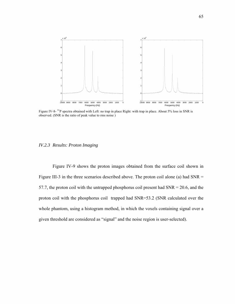
Figure IV-8- 31P spectra obtained with Left: no trap in place Right: with trap in place. About 5% loss in SNR is observed. (SNR is the ratio of peak value to rms noise )
IV.2.3 Results: Proton Imaging
Figure IV-9 shows the proton images obtained from the surface coil shown in
Figure III-3 in the three scenarios described above. The proton coil alone (a) had SNR =
57.7, the proton coil with the untrapped phosphorus coil present had SNR = 20.6, and the
proton coil with the phosphorus coil trapped had SNR=53.2 (SNR calculated over the
whole phantom, using a histogram method, in which the voxels containing signal over a
given threshold are considered as “signal” and the noise region is user-selected).
010002000300040005000600070008000900010000-1
0
1
2
3
4
5
6
7x 10⁶
Frequency (Hz)010002000300040005000600070008000900010000
-1
0
1
2
3
4
5
6
7x 10⁶
Frequency (Hz)
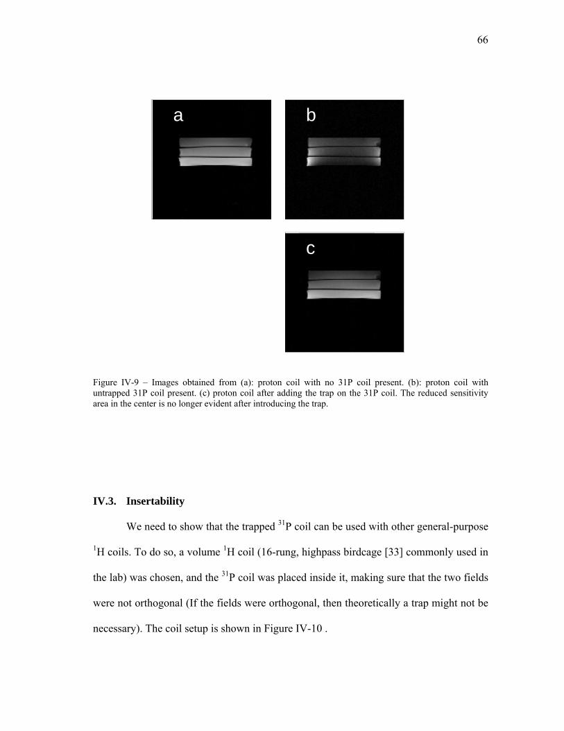
66
Figure IV-9 – Images obtained from (a): proton coil with no 31P coil present. (b): proton coil with untrapped 31P coil present. (c) proton coil after adding the trap on the 31P coil. The reduced sensitivity area in the center is no longer evident after introducing the trap.
IV.3. Insertability
We need to show that the trapped 31P coil can be used with other general-purpose
1H coils. To do so, a volume 1H coil (16-rung, highpass birdcage [33] commonly used in
the lab) was chosen, and the 31P coil was placed inside it, making sure that the two fields
were not orthogonal (If the fields were orthogonal, then theoretically a trap might not be
necessary). The coil setup is shown in Figure IV-10 .
a b
c
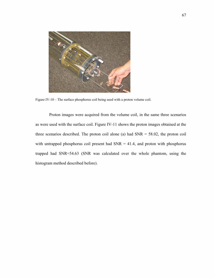
67
Figure IV-10 – The surface phosphorus coil being used with a proton volume coil.
Proton images were acquired from the volume coil, in the same three scenarios
as were used with the surface coil. Figure IV-11 shows the proton images obtained at the
three scenarios described. The proton coil alone (a) had SNR = 58.02, the proton coil
with untrapped phosphorus coil present had SNR = 41.4, and proton with phosphorus
trapped had SNR=54.63 (SNR was calculated over the whole phantom, using the
histogram method described before).

68
Table 3 summarizes the effect of the trap on the SNR of each coil.
Table 3 – Relative SNR obtained at different configurations
Configuration Normalized SNR Surface Proton Coil
Single coil 1.0 Dual coil, no trap 0.36 Dual coil, trapped 0.93
Volume Proton Coil
Single coil 1.0 Dual coil, no trap 0.71 Dual coil, trapped 0.95
Phosphorus Coil
No trap 1.0 With trap 0.95
Figure IV-11 - Images obtained from a proton volume coil. (a) no 31P coil present (b) untrapped 31P coil present, showing reduced sensitivity (c) trapped 31P coil present.
a b
c
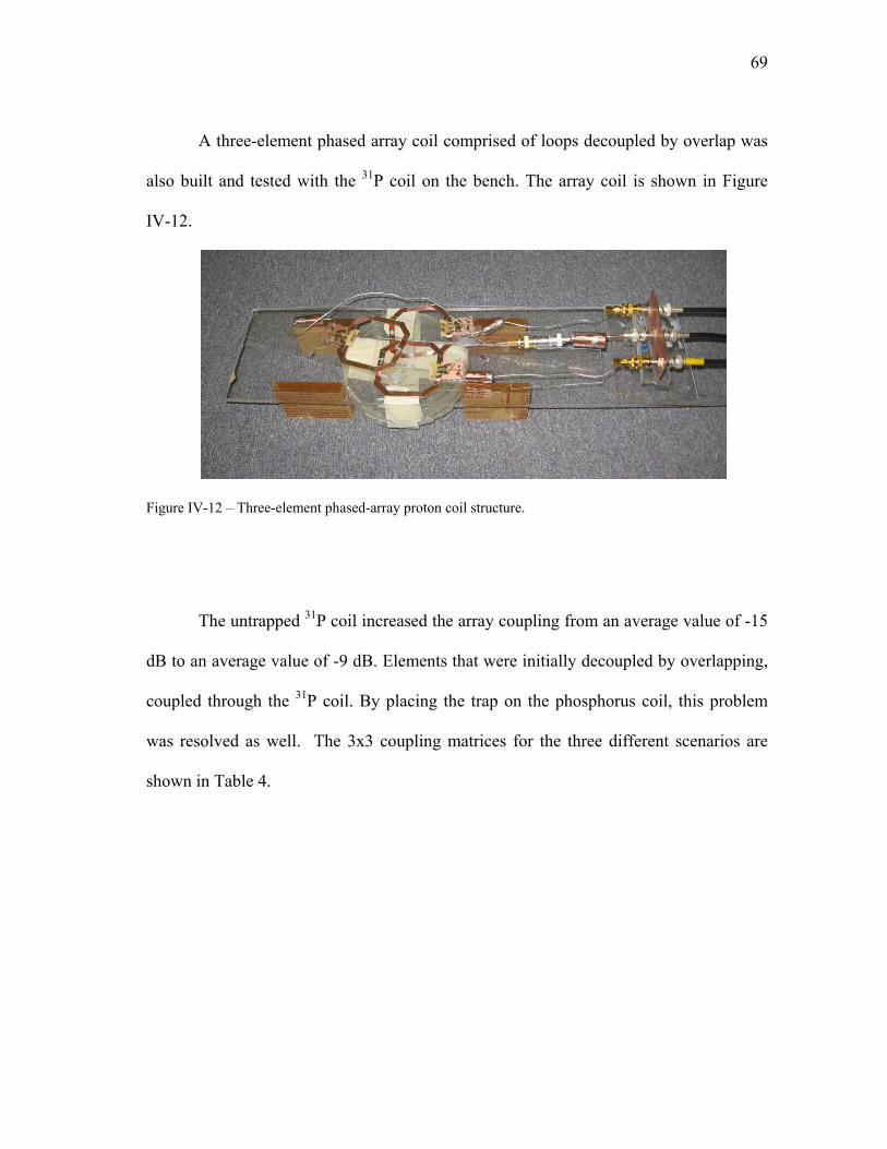
69
A three-element phased array coil comprised of loops decoupled by overlap was
also built and tested with the 31P coil on the bench. The array coil is shown in Figure
IV-12.
Figure IV-12 – Three-element phased-array proton coil structure.
The untrapped 31P coil increased the array coupling from an average value of -15
dB to an average value of -9 dB. Elements that were initially decoupled by overlapping,
coupled through the 31P coil. By placing the trap on the phosphorus coil, this problem
was resolved as well. The 3x3 coupling matrices for the three different scenarios are
shown in Table 4.
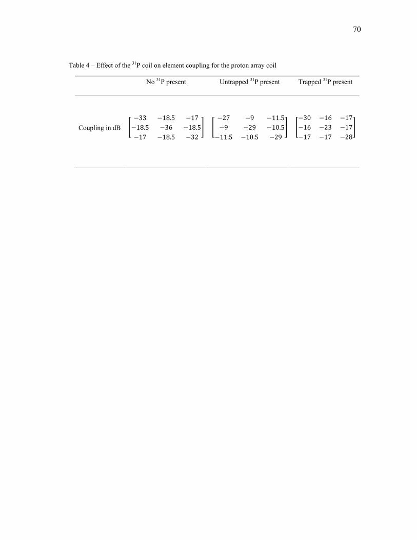
70
Table 4 – Effect of the 31P coil on element coupling for the proton array coil
No 31P present Untrapped 31P present Trapped 31P present
Coupling in dB 33 18.5 17
18.5 36 18.517 18.5 32
27 9 11.59 29 10.5
11.5 10.5 29
30 16 1716 23 1717 17 28
71
CHAPTER V
CONCLUSIONS AND FUTURE WORK
Multi-nuclear MRI and MRS are becoming more prevalent, particularly as MRI
field strengths increase, and with it, the promise of clinical spectroscopy. This will
demand high-performance, versatile multi-frequency probes. In addition, as field
strengths of whole-body magnets increase, proton coil designs are becoming
increasingly specialized, usually entailing the use of complex multi-channel array coils
that cannot easily be re-engineered for multi-frequency use. In this work, a particular
design for a second-nuclei coil using LC traps was implemented and thoroughly
examined. A model was developed to analyze the effect of the trap on resonance
frequency and SNR of both channels. Experimental MR data was obtained to investigate
the performance of this method compared to untrapped cases. The results, which showed
a significant degraded sensitivity of the proton coil when an untrapped phosphorus coil
was present, explain why untrapped, concentric designs for proton decoupling usually
fail to achieve FDA limits for SAR, as the power input to the proton coil is increased in
order to compensate for the decreased sensitivity. Also, applicability of the trap method
was examined to enable using second-nuclei coils in conjunction with existing proton
coils, saving the cost of designing specialized proton coils. Guidelines are provided for
trap design, in order to further enhance the performance and insertability.
In general, when migrating from a single-tuned to dual-tuned coil system,
performance loss for at least one of the nuclei is unavoidable (regardless of the dual-

72
tuning scheme used). Methods used in the past usually provide guidelines to optimize
the design in favor of the observation channel (less-abundant nuclei), imposing a
significant loss (on the order of 50%) on the proton channel. We showed that by using
the trap design, performance at both nuclear frequencies can be maintained above 90%
of their single-tuned counterparts. Our lab is known for its work in parallel imaging –
both multichannel receive and transmit hardware and methodology. The insertability of a
second-nuclei coil enabled by the use of a trap should allow for more straightforward
incorporation of spectroscopy studies into our lab’s existing array coil studies, opening
the way for a variety of future work, such as in vivo 31P magnetic resonance
spectroscopy. Also, this method is applicable in higher frequency RF coil designs, of
particular interest with the increasing availability of higher field magnets.

73
REFERENCES
[1] T. Toyooka, K. Nagayama, J. Suzuki, and T. Sugimoto, Noninvasive assessment of
cardiomyopathy development with simultaneous measurement of topical H-1 and P-31 magnetic resonance spectroscopy. Circulation 86 (1992) 295-301.
[2] P.A. Bottomley, and R.G. Weiss, Non-invasive magnetic-resonance detection of
creatine depletion in non-viable infarcted myocardium. Lancet 351 (1998) 714-718.
[3] J.W. Hugg, G.B. Matson, D.B. Twieg, A.A. Maudsley, D. Sappeymarinier, and
M.W. Weiner, P-31 MR spectroscopic imaging (MRSI) of normal and pathological human brains. Magnetic Resonance Imaging 10 (1992) 227-243.
[4] W. Negendank, Studies of human tumors by MRS - a review. NMR in Biomedicine
5 (1992) 303-324. [5] D.J. Griffiths, Introduction to electrodynamics, Prentice Hall, Upper Saddle River,
NJ, 1999. [6] A.J. Shaka, J. Keeler, T. Frenkiel, and R. Freeman, An improved sequence for
broad-band decoupling - Waltz-16. Journal of Magnetic Resonance 52 (1983) 335-338.
[7] H. Bomsdorf, P. Roschmann, and J. Wieland, Sensitivity enhancement in whole-
body natural abundance C-13 spectroscopy ssing C-13/H-1 double-resonance techniques at 4-Tesla. Magnetic Resonance in Medicine 22 (1991) 10-22.
[8] M.D. Schnall, V.H. Subramanian, J.S. Leigh, and B. Chance, A new double-tuned
probe for concurrent H-1 and P-31 NMR. Journal of Magnetic Resonance 65 (1985) 122-129.
[9] M. Schnall, NMR, basic principles and progress. Edited by Diehl, P, Springer-
Verlag, Berlin, 1992. [10] M. Decorps, P. Blondet, H. Reutenauer, J.P. Albrand, and C. Remy, An Inductively
coupled, series-tuned NMR probe. Journal of Magnetic Resonance 65 (1985) 100-109.
[11] D.I. Hoult, and B. Tomanek, Use of mutually inductive coupling in probe design.
Concepts in Magnetic Resonance 15 (2002) 262-285.

74
[12] D.I. Hoult, The NMR receiver: A description and analysis of design. Progress in Nuclear Magnetic Resonance Spectroscopy 12 (1978) 41-77.
[13] G.B. Matson, P. Vermathen, and T.C. Hill, A practical double-tuned H-1/P-31
quadrature birdcage headcoil optimized for P-31 operation. Magnetic Resonance in Medicine 42 (1999) 173-182.
[14] J. Murphyboesch, R. Srinivasan, L. Carvajal, and T.R. Brown, Two configurations
of the four-ring birdcage coil for 1H imaging and 1H-decoupled 31P spectroscopy of the human head. Journal of Magnetic Resonance, Series B 103 (1994) 103-114.
[15] V.R. Cross, R.K. Hester, and J.S. Waugh, Single coil probe with transmission-line
tuning for nuclear magnetic double-resonance. Review of Scientific Instruments 47 (1976) 1486-1488.
[16] M.E. Stoll, A.J. Vega, and R.W. Vaughan, Simple single-coil double-resonance
NMR probe for solid-state studies. Review of Scientific Instruments 48 (1977) 800-803.
[17] G. Annaert, A. Barel, R. Luypaert, M. Osteaux, and J. Renneboog, A low-lossy
double tuned resonator for concurrent 1H and 31P nuclear magnetic resonance, Instrumentation and Measurement Technology Conference, 1989. IMTC-89. Conference Record., 6th IEEE, 1989, pp. 190-193.
[18] F.D. Doty, R.R. Inners, and P.D. Ellis, A multi-nuclear double-tuned probe for
applications with solids or liquids utilizing lumped tuning elements. Journal of Magnetic Resonance 43 (1981) 399-416.
[19] J.R. Fitzsimmons, H.R. Brooker, and B. Beck, A transformer-coupled double-
resonant probe for NMR imaging and spectroscopy. Magnetic Resonance in Medicine 5 (1987) 471-477.
[20] J.R. Fitzsimmons, B.L. Beck, and H.R. Brooker, Double resonant quadrature
birdcage. Magnetic Resonance in Medicine 30 (1993) 107-114. [21] P.A. Bottomley, C.J. Hardy, P.B. Roemer, and O.M. Mueller, Proton-decoupled,
Overhauser-enhanced, spatially-localized C-13 spectroscopy in humans. Magnetic Resonance in Medicine 12 (1989) 348-363.
[22] H. Merkle, H.R. Wei, M. Garwood, and K. Ugurbil, B1-insensitive heteronuclear
adiabatic polarization transfer for signal enhancement. Journal of Magnetic Resonance 99 (1992) 480-494.
75
[23] G. Adriany, and R. Gruetter, A half-volume coil for efficient proton decoupling in humans at 4 Tesla. Journal of Magnetic Resonance 125 (1997) 178-184.
[24] W. Durr, and S. Rauch, A dual-frequency circularly polarizing whole-body MR
antenna for 69/170 MHz. Magnetic Resonance in Medicine 19 (1991) 446-455. [25] M. Alecci, S. Romanzetti, J. Kaffanke, A. Celik, H.P. Wegener, and N.J. Shah,
Practical design of a 4 Tesla double-tuned RF surface coil for interleaved H-1 and Na-23 MRI of rat brain. Journal of Magnetic Resonance 181 (2006) 203-211.
[26] S.M. Wright, and L.L. Wald, Theory and application of array coils in MR
spectroscopy. Nmr in Biomedicine 10 (1997) 394-410. [27] J. Mispelter, B. Tiffon, E. Quiniou, and J.M. Lhoste, Optimization of C-13-(H-1)
double coplanar surface-coil design for the waltz-16 decoupling sequence. Journal of Magnetic Resonance 82 (1989) 622-628.
[28] F.W. Grover, Inductance calculations, working formulas and tables, D. Van
Nostrand company, inc., New York, 1946. [29] G.B. Peter R. Luyten, Frenk M. Sloff, Jan W. A. H. Vermeulen, Jan I. Van Der
Heijden, Jan A. Den Hollander, Arend Heerschap, Broadband proton decoupling in human 31P NMR spectroscopy. NMR in Biomedicine 1 (1989) 177-183.
[30] K. Hendrich, H.Y. Liu, H. Merkle, J. Zhang, and K. Ugurbil, B1 voxel shifting of
phase-modulated spectroscopic localization techniques. Journal of Magnetic Resonance 97 (1992) 486-497.
[31] M. Garwood, and K. Yong, Symmetrical pulses to induce arbitrary flip angles with
compensation for RF inhomogeneity and resonance offsets. Journal of Magnetic Resonance 94 (1991) 511-525.
[32] R.A. De Graaf, In vivo NMR spectroscopy : principles and techniques, Wiley,
Chichester ; New York, 1998. [33] M.P. McDougall, D.G. Brown, D.K. Spence, and S.M. Wright, A low-pass
trombone birdcage coil with broad tuning range, Proc. Intl. Soc. Mag. Reson. Med, 2001, pp. 1092.
76
VITA
Arash Dabirzadeh was born in Esfahan, Iran in 1982. He received his Bachelor of
Science degree with honors in Electrical Engineering from Amirkabir University of
Technology (Tehran Polytechnic) in 2005 and Master of Science degree in Electrical
Engineering from Texas A&M University in 2008. His research/career interests include
RF/microwave circuit/coil design for medical imaging.
Mr. Dabirzadeh may be reached at the Department of Electrical and Computer
Engineering, 111A Zachry Engineering Building, College Station, TX 77843-3128 or
via email at [email protected].


