RF Channel & Modulation Fundamentals - Wirelesswireless.ictp.it/wp-content/uploads/2012/02/1... ·...

RF Channel & Modulation Fundamentals

Prof. Ryszard Struzak National Institute of Telecommunications, Poland

r.struzakATieee.org

The Abdus Salam International Centre for Theoretical Physics ICTP-ITU/BDT School on Sustainable Wireless ICT Solutions for Environmental Monitoring

6 – 22 February 2012, ICTP, Miramare-Trieste, Italy

(CC) R Struzak <[email protected]> 2

Objective

•  Review of basic physical processes involved in modern communication systems that may be needed to understand better the further training/teaching activities at ICTP


Topics for discussion

•  Radio transmission •  Modulation schemes •  Constellation diagrams •  Modulation spectra


http://ursi.org/files/RSBissues/RSB_339_2011_12.pdf

(CC) R Struzak <[email protected]> 5 Source: URSI RSB No 339 Dec. 2011


Source: URSI RSB No 339 Dec. 2011


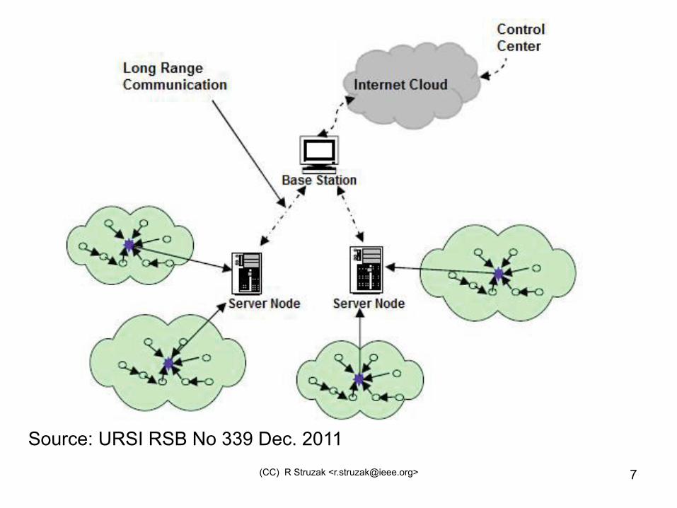
Radio Transmission System •  A message, from a source of messages, is delivered to a

distant destination via radio communication channel using energy of radio waves

»  Message in its most general meaning is the object of communication. Depending on the context, the term may apply to both the information contents and its actual presentation, or signal.

»  The baseband signal usually consist of a finite set of symbols. E.g. text message is composed of words that belong to a finite vocabulary of the language used. Each word in turn is composed by letters of a (finite) alphabet. (Analog-to-digital conversion)

»  The channel consists of a transmitter node, radio propagation path and receiver node.

•  The radio propagation process distorts the signal »  Predictable vs unpredictable distortions

•  The transmitter & receiver pair process the signal to repair the signal distortions following common communication protocol and communication policy


Volume of information transmitted by isolated communication channel

C = B*log2{1 + [S/(No*B)]}

Bandwidth, Hz

Noise power density, W/Hz Received signal power, W

Capacity (maximum throughput), bit-per-second • The capacity to transfer error-free information is enhanced

with increased bandwidth B, even though the signal-to-noise ratio is decreased because of the increased bandwidth.

• C/B (bps/Hz) → bandwidth efficiency

•  The actual throughput can only approach the channel capacity using an extremely complicated encoder. –  The statistical properties of the signal approach those

of Gaussian noise and the coding time increases indefinitely.

–  Rice (1950) has shown that in order to achieve a data rate which is 96 percent of the channel capacity with S/NoB = 10 and an error probability of 10-5 the number of block encoded channel signals required is 210,000. This is just as impractical as theinfinite coding delay required.

•  Source: R. F. Linfield: Radio Channel Capacity Limitations; ITS NTIA



Time division headers; interactive & real-time applications that require acknowledgment!

V

Freq

uenc

y sl

ot B

Time slot T

V = B*T*log2{1 + [S/(No*B)]}

Frequency division


FDD radio links •  Two stations can talk and listen to each other at the

same time (time-sharing). •  This requires separate synchronized frequency channels

– a technique known as Frequency Division Duplex (FDD)

Station 1 Station 2

FrequencyChannel 1

Frequency Channel 2 TX RX

TX RX


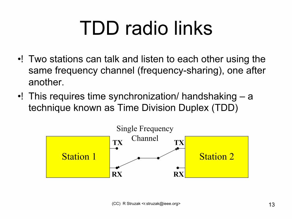
TDD radio links •  Two stations can talk and listen to each other using the

same frequency channel (frequency-sharing), one after another.

•  This requires time synchronization/ handshaking – a technique known as Time Division Duplex (TDD)

Station 1 Station 2

Single Frequency Channel TX

RX

TX

RX


Broadband (INTEL: 100+ Mbps)

INTEL opinion: 100 Mbps necessary! Ch. Legutko (Intel Corp. Wireless Standards & Regulations Mngr): „Regulatory & Spectrum”; presentation, Broadband Forum, Warsaw, July 2006


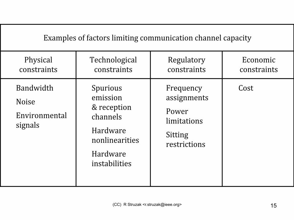
!"#$%&'()*+)+#,-*.()&/$/-/01),*$$20/,#-/*0),3#00'&),#%#,/-4))

534(/,#&)),*0(-.#/0-()

6',30*&*1/,#&),*0(-.#/0-()

7'12&#-*.4),*0(-.#/0-()

!,*0*$/,)))))),*0(-.#/0-()

8#09:/9-3);*/(')!0</.*0$'0-#&)(/10#&()

=%2./*2()'$/((/*0))>).','%-/*0),3#00'&()?#.9:#.')0*0&/0'#./-/'()?#.9:#.')/0(-#@/&/-/'())

A.'B2'0,4)#((/10$'0-()5*:'.)&/$/-#-/*0()=/--/01).'(-./,-/*0()

C*(-))

)

•  The fundamental physical limitations are bandwidth and noise.

•  The bandwidth limits the number of signaling elements or symbols which can be transmitted per unit time.

•  The noise limits the number of distinguishable features on each symbol.

•  The combined effects limit the capacity of a communication system.



Envi

ronm

ent

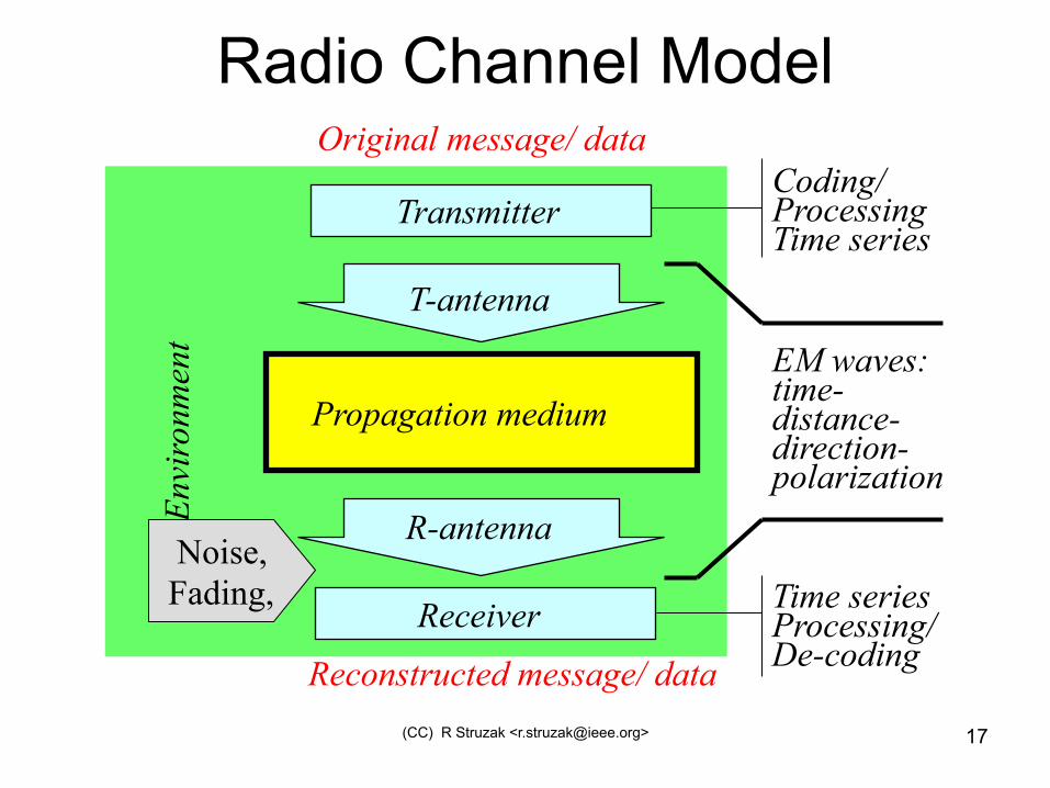
Radio Channel Model

T-antenna

Propagation medium

R-antenna Noise, Fading,

Original message/ data

Reconstructed message/ data

EM waves: time- distance- direction- polarization

Receiver Time series Processing/ De-coding

Transmitter Coding/ Processing Time series


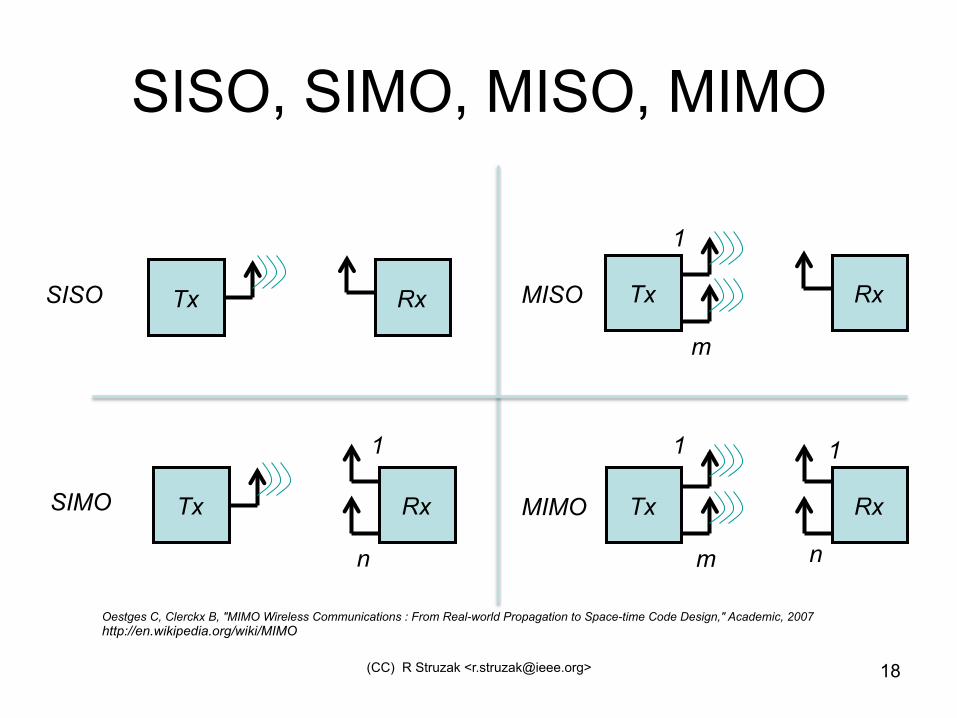
SISO, SIMO, MISO, MIMO

Tx Rx SISO

Tx Rx SIMO

1

n

Tx Rx

1

m

MISO

Tx Rx

n

1 1

m

MIMO

Oestges C, Clerckx B, "MIMO Wireless Communications : From Real-world Propagation to Space-time Code Design," Academic, 2007 http://en.wikipedia.org/wiki/MIMO


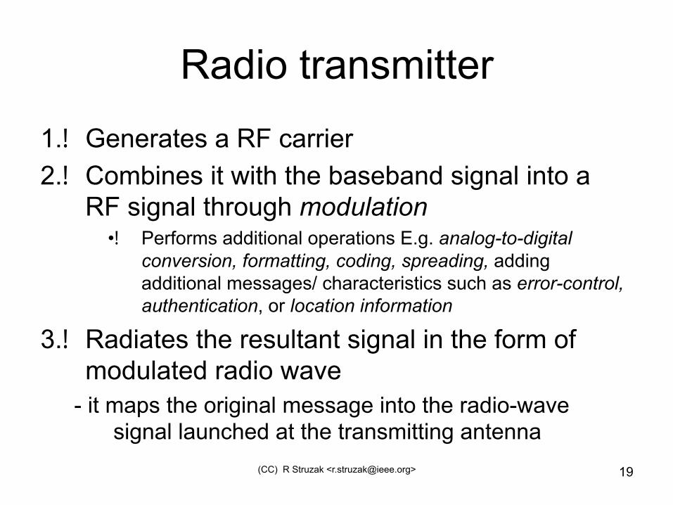
Radio transmitter

1.  Generates a RF carrier 2.  Combines it with the baseband signal into a

RF signal through modulation •  Performs additional operations E.g. analog-to-digital

conversion, formatting, coding, spreading, adding additional messages/ characteristics such as error-control, authentication, or location information

3.  Radiates the resultant signal in the form of modulated radio wave

- it maps the original message into the radio-wave signal launched at the transmitting antenna


Propagation process

•  Transforms (maps) the radio-wave launched by the transmitter into the incident radio wave at the receiver antenna

•  Depends on extra variables (e.g. distance), additional radio waves (e.g. reflected wave, environmental waves), random uncertainty additive (noise), multiplicative (fading), etc.

•  A separate talk


Radio receiver: 1.  Extracts the wanted signal from the

incident radio waves (a solid “window” in the signal hyperspace)

2.  Recovers the original message through •  reversing the transmitter operations

(demodulation, decoding, de-spreading, etc.),

•  compensating propagation transformations, and

•  correcting transmission distortions

•  Maps the incident signals into the recovered message

•  Coexistence - Separate talk!

Receiver +

Wanted signal

Unwanted signals

Noise

Unwanted signals and nonlinearities are often ignored!


Modulation & Demodulation

•  Modulation - translation the baseband message signal to radio frequencies

•  Demodulation -- the reverse process) – Single carrier:

•  continuous (sinusoidal), •  Walsh functions (http://mathworld.wolfram.com/WalshFunction.html)

•  Random carriers (http://en.wikipedia.org/wiki/Category:Radio_modulation_modes) – Multiple carriers (e.g. OFDM)


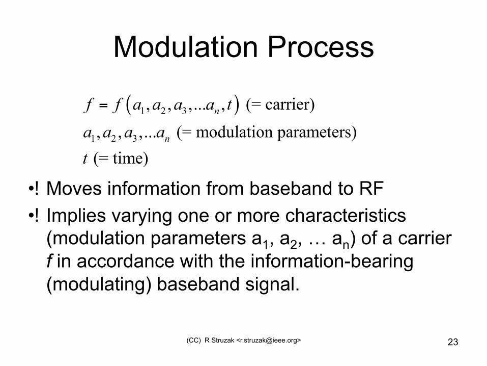
Modulation Process

•  Moves information from baseband to RF •  Implies varying one or more characteristics

(modulation parameters a1, a2, … an) of a carrier f in accordance with the information-bearing (modulating) baseband signal.

( )1 2 3

1 2 3

, , ,... , (= carrier), , ,... (= modulation parameters)

(= time)

n

n

f f a a a a ta a a at

=


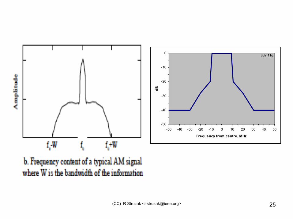
Frequency translation

•  Signal "at baseband" comprises all frequency components carrying information. Modulation shifts the signal up to RF frequencies to allow for radio transmission. Usually, the process increases the signal bandwidth. Steps are often taken to reduce this effect, such as filtering the RF signal prior to transmission.

Signal's baseband bandwidth is its bandwidth before modulation and multiplexing, or after demultiplexing and demodulation


-50

-40

-30

-20

-10

0

-50 -40 -30 -20 -10 0 10 20 30 40 50

Frequency from centre, MHz

dB

802.11g


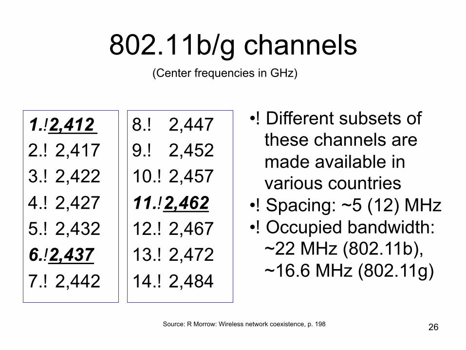
802.11b/g channels

1.  2,412 2.  2,417 3.  2,422 4.  2,427 5.  2,432 6.  2,437 7.  2,442

8.  2,447 9.  2,452 10.  2,457 11.  2,462 12.  2,467 13.  2,472 14.  2,484

•  Different subsets of these channels are made available in various countries •  Spacing: ~5 (12) MHz •  Occupied bandwidth: ~22 MHz (802.11b), ~16.6 MHz (802.11g)

(Center frequencies in GHz)

Source: R Morrow: Wireless network coexistence, p. 198


Why translation?

•  Effective radiation of EM energy requires antenna dimensions to be comparable with the wavelength: – 3 kHz: wavelength 100 km – 3 GHz: wavelength 10 cm

•  Allows shared use of the radio transmission medium


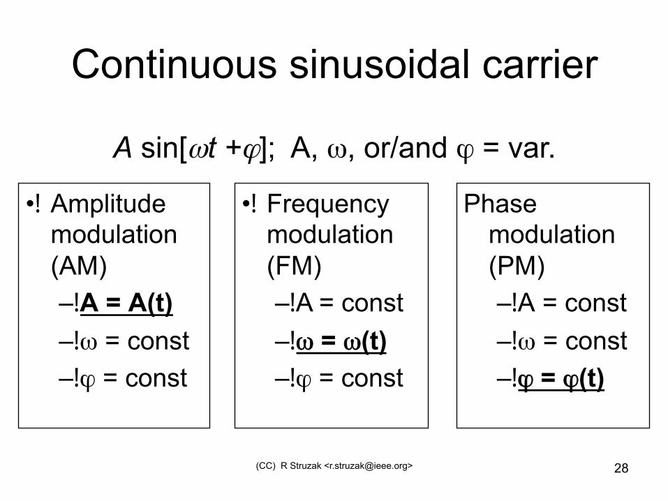
Continuous sinusoidal carrier

•  Amplitude modulation (AM) – A = A(t) – ω = const – ϕ = const

Phase modulation (PM) – A = const – ω = const – ϕ = ϕ(t)

A sin[ωt +ϕ]; A, ω, or/and ϕ = var.

•  Frequency modulation (FM) – A = const – ω = ω(t) – ϕ = const


AM, FM, PM

The modulating signal superimposed on the carrier wave & the resulting modulated signal. [wikipedia]

Java simulation: http://www.home.agilent.com/upload/cmc_upload/All/Amplitude_Modulation.htm?cmpid=zzfindnw_amplitudemod


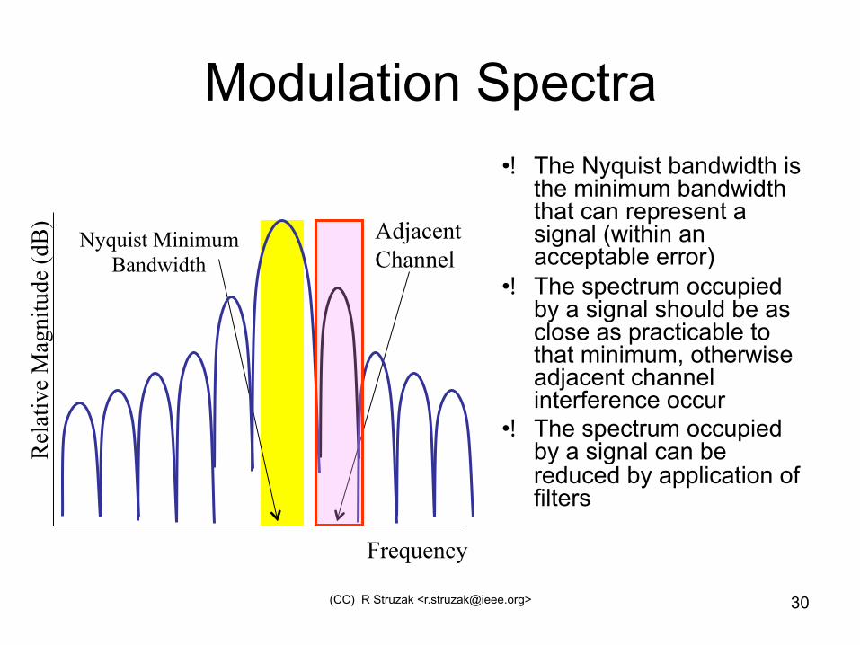
Modulation Spectra •  The Nyquist bandwidth is

the minimum bandwidth that can represent a signal (within an acceptable error)

•  The spectrum occupied by a signal should be as close as practicable to that minimum, otherwise adjacent channel interference occur

•  The spectrum occupied by a signal can be reduced by application of filters

Nyquist Minimum Bandwidth

Frequency

Rel

ativ

e M

agni

tude

(dB

) Adjacent Channel


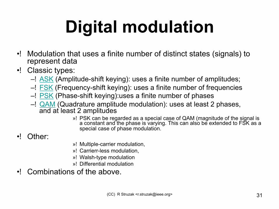
Digital modulation •  Modulation that uses a finite number of distinct states (signals) to

represent data •  Classic types:

–  ASK (Amplitude-shift keying): uses a finite number of amplitudes; –  FSK (Frequency-shift keying): uses a finite number of frequencies –  PSK (Phase-shift keying):uses a finite number of phases –  QAM (Quadrature amplitude modulation): uses at least 2 phases,

and at least 2 amplitudes »  PSK can be regarded as a special case of QAM (magnitude of the signal is

a constant and the phase is varying. This can also be extended to FSK as a special case of phase modulation.

•  Other: »  Multiple-carrier modulation, »  Carrierr-less modulation, »  Walsh-type modulation »  Differential modulation

•  Combinations of the above.


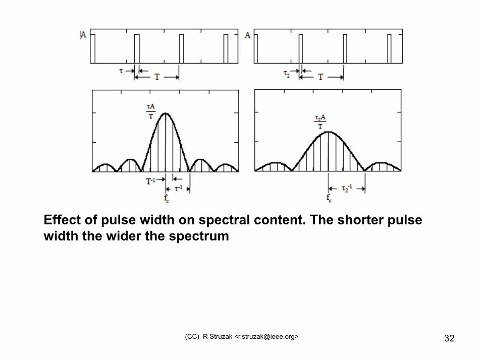
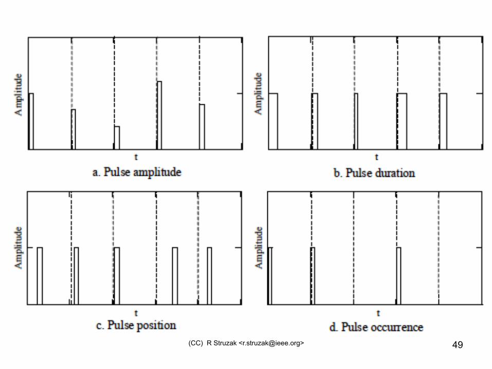
Effect of pulse width on spectral content. The shorter pulse width the wider the spectrum


Differential Modulation •  At transmitter: each symbol is modulated

relative to the previous symbol and modulating data

•  DPSK (Differential Phase-Shift Keying) example: 0 = no change; 1 = change phase by +1800

•  At receiver: the current symbol is reproduced using the previous symbol as reference.

•  The previous symbol serves as an estimate of the channel. A no-change condition causes the modulated signal to remain at the same 0 or 1 state as the previous symbol.

•  Differential modulation has 2 sources of error: •  a corrupted current symbol, and corrupted reference (the

previous symbol)


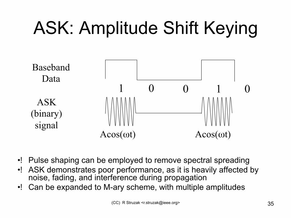
ASK: Amplitude Shift Keying

•  Pulse shaping can be employed to remove spectral spreading •  ASK demonstrates poor performance, as it is heavily affected by

noise, fading, and interference during propagation •  Can be expanded to M-ary scheme, with multiple amplitudes

Baseband Data

ASK (binary) signal

1 1 0 0 0

Acos(ωt) Acos(ωt)


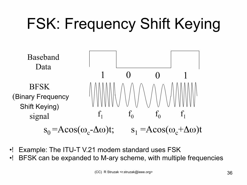
FSK: Frequency Shift Keying

•  Example: The ITU-T V.21 modem standard uses FSK •  BFSK can be expanded to M-ary scheme, with multiple frequencies

Baseband Data

BFSK (Binary Frequency

Shift Keying) signal

1 1 0 0

s0 =Acos(ωc-Δω)t; s1 =Acos(ωc+Δω)t

f0 f0 f1 f1


PSK: Phase Shift Keying

•  BPSK – better performance than ASK and BFSK •  Drawback: rapid amplitude change between symbols due to phase

discontinuity requires infinite bandwidth. •  BPSK can be expanded to M-ary scheme, with multiple phases

Baseband Data

BPSK (Binary Phase Shift Keying)

signal

1 1 0 0

s0 =-Acos(ωct); s1 =Acos(ωct) s0 s0 s1 s1


•  Phase Shift Keying (PSK) is often used as it provides efficient use of RF spectrum. π/4 QPSK (Quadrature PSK) reduces the envelope variation of the signal.

•  High level M-array schemes (such as 64-QAM) are bandwidth-efficient but susceptible to noise and require linear amplification

•  Constant envelope schemes (e.g. GMSK) allow for non-linear power-efficient amplifiers

•  Coherent reception provides better performance but requires a more complex receiver


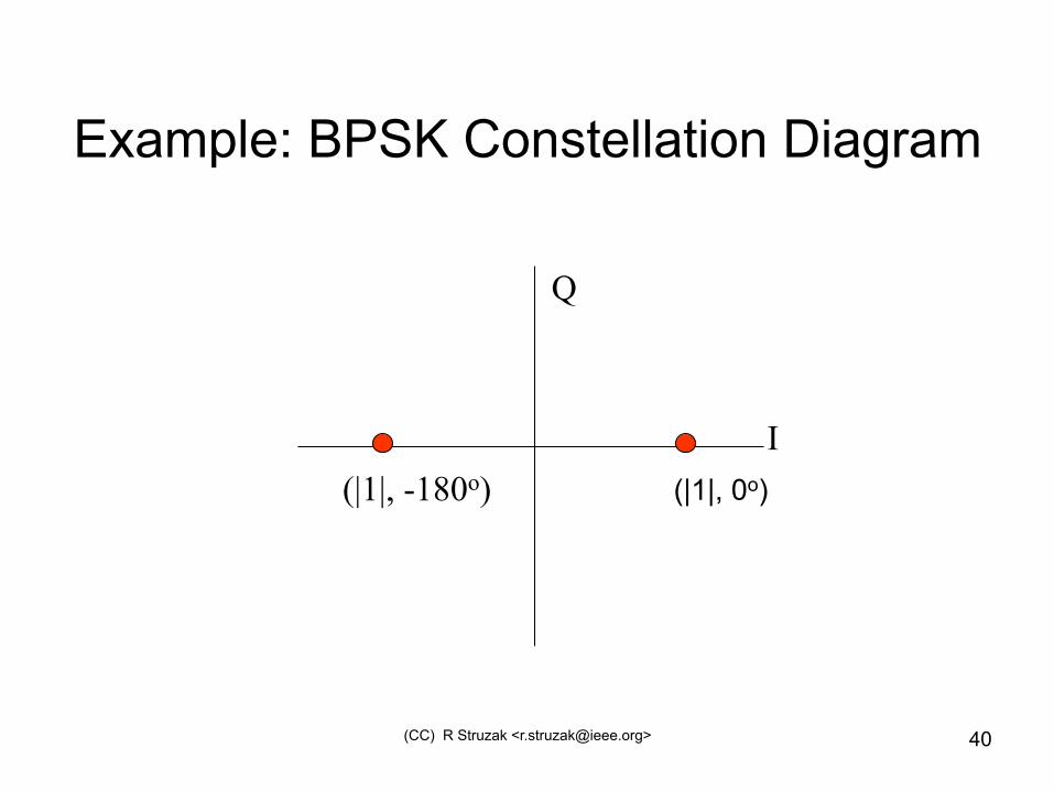
Constellation diagram

= graphical representation of the amplitude and phase of each possible symbol state in time domain – The x-axis represents the in-phase

component and the y-axis the quadrature component of the complex envelope

– The distance between signal states on a constellation diagram indicates

•  how different the modulation waveforms are •  how easily a receiver can differentiate between

them.


Example: BPSK Constellation Diagram

(|1|, -180o)

Q

I (|1|, 0o)


QPSK

•  Quadrature Phase Shift Keying (QPSK) can be interpreted as two independent BPSK systems (one on the I-channel and one on Q), and thus the same performance but twice the bandwidth efficiency

•  Large envelope variations occur due to abrupt phase transitions, thus requiring linear amplification


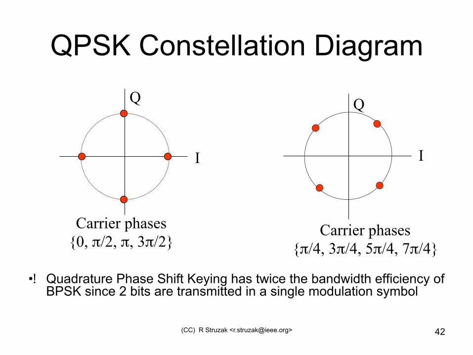
QPSK Constellation Diagram

•  Quadrature Phase Shift Keying has twice the bandwidth efficiency of BPSK since 2 bits are transmitted in a single modulation symbol

Carrier phases {0, π/2, π, 3π/2}

Carrier phases {π/4, 3π/4, 5π/4, 7π/4}

Q

I I

Q


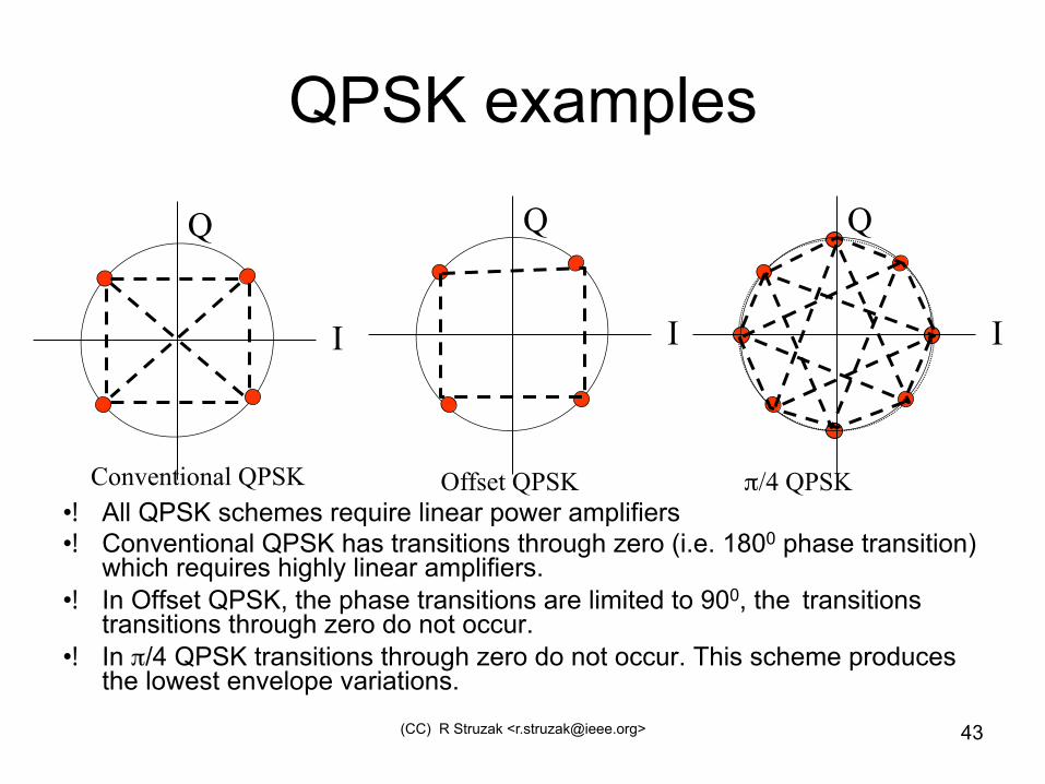
QPSK examples

•  All QPSK schemes require linear power amplifiers •  Conventional QPSK has transitions through zero (i.e. 1800 phase transition)

which requires highly linear amplifiers. •  In Offset QPSK, the phase transitions are limited to 900, the transitions

transitions through zero do not occur. •  In π/4 QPSK transitions through zero do not occur. This scheme produces

the lowest envelope variations.

I

Q

I

Q

I

Q

Conventional QPSK π/4 QPSK Offset QPSK


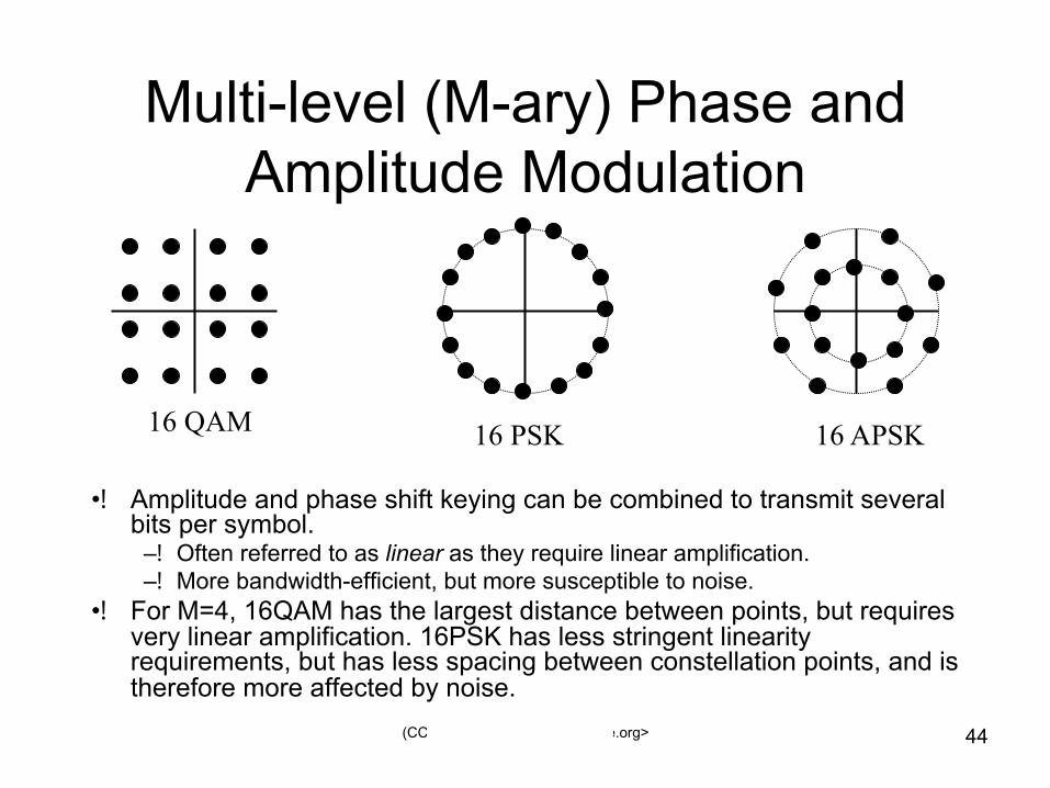
Multi-level (M-ary) Phase and Amplitude Modulation

•  Amplitude and phase shift keying can be combined to transmit several bits per symbol.

–  Often referred to as linear as they require linear amplification. –  More bandwidth-efficient, but more susceptible to noise.

•  For M=4, 16QAM has the largest distance between points, but requires very linear amplification. 16PSK has less stringent linearity requirements, but has less spacing between constellation points, and is therefore more affected by noise.

16 QAM 16 APSK 16 PSK


•  Animations:

•  http://www.home.agilent.com/upload/cmc_upload/All/IQ_Modulation.htm?cmpid=zzfindnw_iqmod

•  http://www.home.agilent.com/agilent/editorial.jspx?cc=PL&lc=eng&ckey=1756523&nid=-34944.0&id=1756523


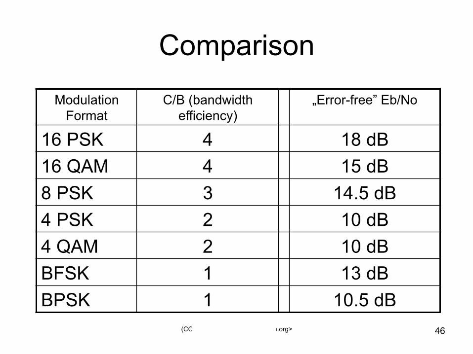
Comparison

Modulation Format

C/B (bandwidth efficiency)

„Error-free” Eb/No

16 PSK 4 18 dB 16 QAM 4 15 dB 8 PSK 3 14.5 dB 4 PSK 2 10 dB 4 QAM 2 10 dB BFSK 1 13 dB BPSK 1 10.5 dB


Distortions

Perfect channel White noise Phase jitter


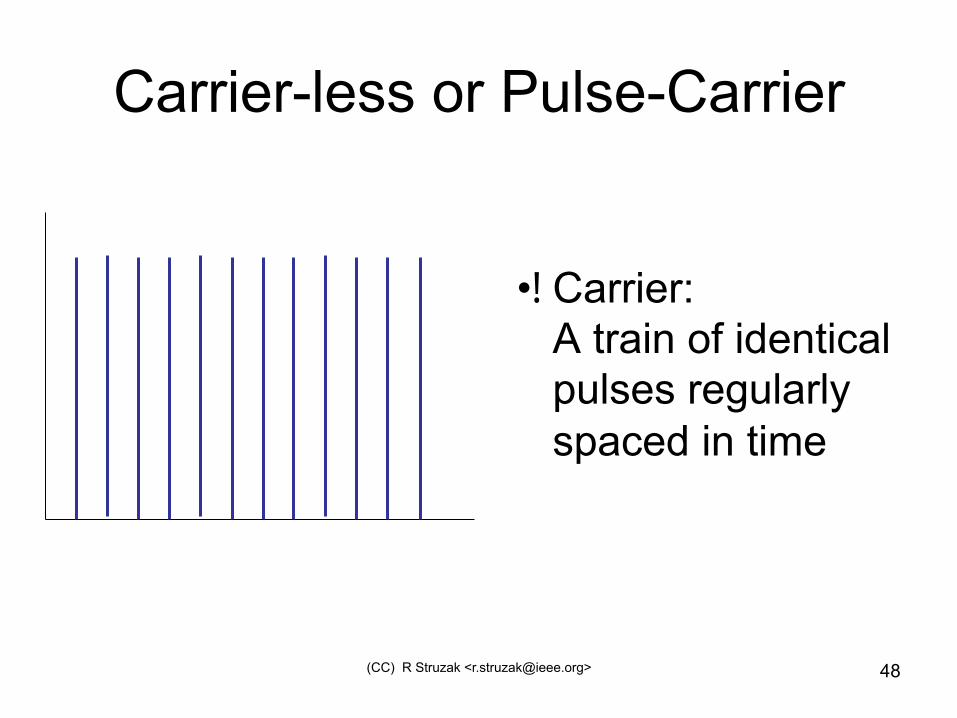
Carrier-less or Pulse-Carrier

•  Carrier: A train of identical pulses regularly spaced in time


Ultra-Wideband (UWB) Systems •  Radio systems that use time-domain processing

(e.g., pulse-position modulation) for communications, or sensing applications. –  e.g. short-range radar; –  Also called carrier-less or impulse systems; –  Occupy frequency bandwidth >25% of the center

frequency or >1.5 GHz. –  Use narrow pulses

•  Of the order of 1 to 10 nanoseconds.


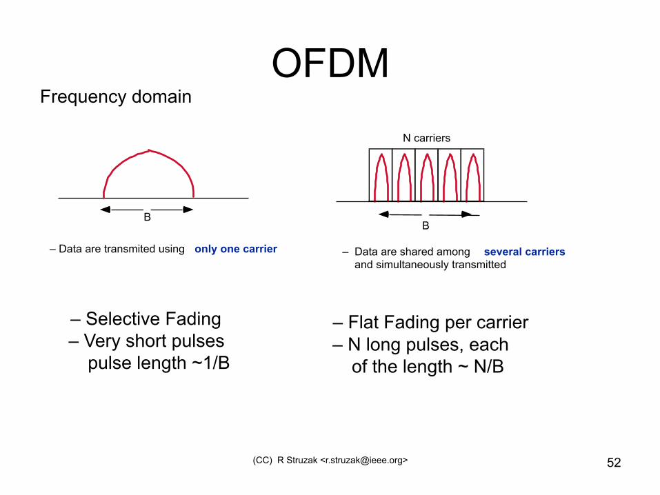
Multiple-carrier systems example •  OFDM = Orthogonal Frequency Division Multiplex •  Basic idea:

–  Using a large number of parallel narrow-band sub-carriers instead of a single wide-band carrier to transport information

•  Advantages –  Efficient in dealing with multi-path and selective fading –  Robust again narrow-band interference

•  Disadvantages –  Sensitive to frequency offset and phase noise –  Peak-to-average problem reduces the power efficiency of RF

amplifier at the transmitter •  Adopted for various standards

•  DSL, 802.11a, DAB, DVB


OFDM

– Selective Fading – Very short pulses

pulse length ~1/B

– Flat Fading per carrier – N long pulses, each

of the length ~ N/B

N carriers

B

– Data are shared among several carriers and simultaneously transmitted

B

– Data are transmited using only one carrier

Frequency domain


OFDM 2 Inverse Fourier

Transform IFFT

Parallel To Serial converter

Serial to Parallel

converter

Fourier Transform

FFT Transmission

Data coded in frequency domain one symbol at a time

Data in time domain one symbol at a time

Transmit time-domain samples of one symbol

Decode each

frequency bin

independently

More information: http://www.iss.rwth-aachen.de/Projekte/Theo/OFDM/node2.html


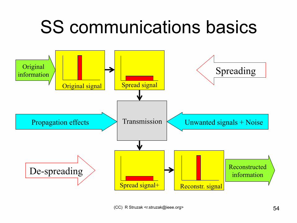
SS communications basics

Original information

Propagation effects Transmission

Reconstructed information

Original signal Spread signal

Spread signal+ Reconstr. signal

Spreading

De-spreading

Unwanted signals + Noise


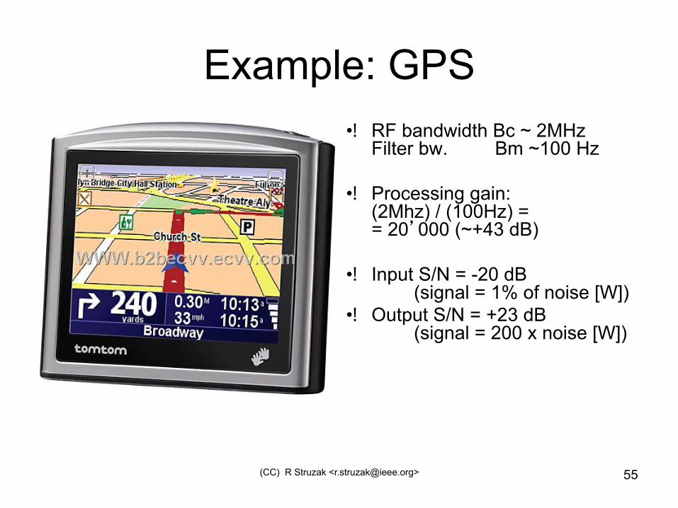
Example: GPS •  RF bandwidth Bc ~ 2MHz

Filter bw. Bm ~100 Hz

•  Processing gain: (2Mhz) / (100Hz) = = 20’000 (~+43 dB)

•  Input S/N = -20 dB (signal = 1% of noise [W])

•  Output S/N = +23 dB (signal = 200 x noise [W])


SS techniques

•  FH: frequency hoping (frequency synthesizer controlled by pseudo-random sequence of numbers)

•  DS: direct sequence (pseudo-random sequence of pulses used for spreading)

•  TH: time hoping (spreading achieved by randomly spacing transmitted pulses)

•  Random noise as carrier •  Other techniques (radar and other applications)

•  Combination of the above


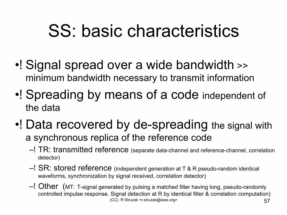
SS: basic characteristics

•  Signal spread over a wide bandwidth >> minimum bandwidth necessary to transmit information

•  Spreading by means of a code independent of the data

•  Data recovered by de-spreading the signal with a synchronous replica of the reference code –  TR: transmitted reference (separate data-channel and reference-channel, correlation

detector)

–  SR: stored reference (independent generation at T & R pseudo-random identical waveforms, synchronization by signal received, correlation detector)

–  Other (MT: T-signal generated by pulsing a matched filter having long, pseudo-randomly controlled impulse response. Signal detection at R by identical filter & correlation computation)


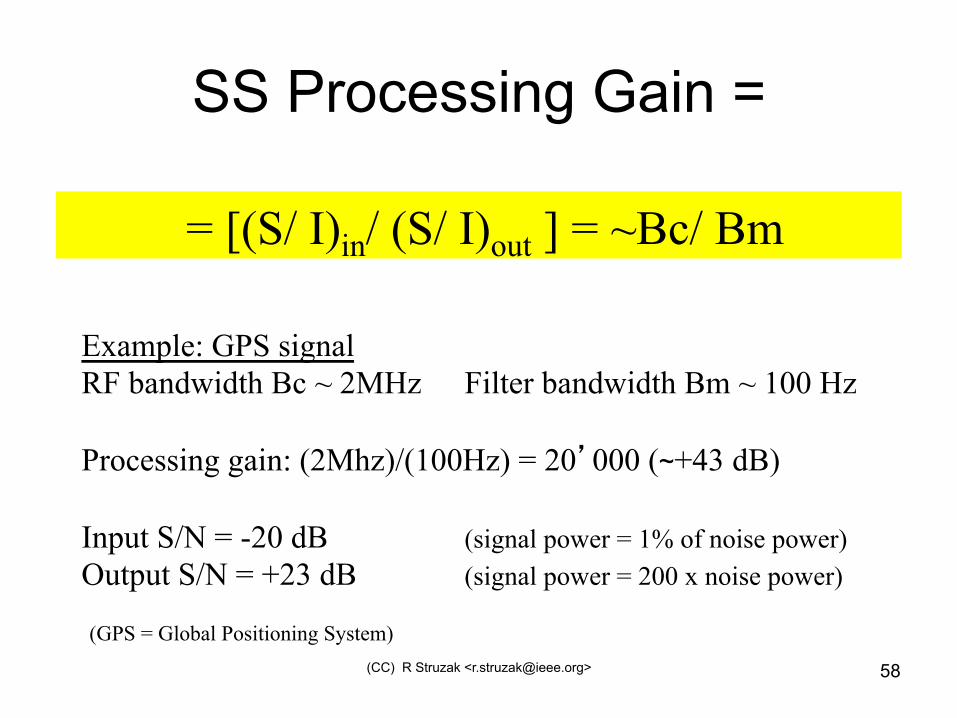
SS Processing Gain =

= [(S/ I)in/ (S/ I)out ] = ~Bc/ Bm

Example: GPS signal RF bandwidth Bc ~ 2MHz Filter bandwidth Bm ~ 100 Hz Processing gain: (2Mhz)/(100Hz) = 20’000 (~+43 dB) Input S/N = -20 dB (signal power = 1% of noise power) Output S/N = +23 dB (signal power = 200 x noise power) (GPS = Global Positioning System)

(CC) R Struzak <r.struzakATieee.org> 59

•  Beware of misprints!!! These materials are preliminary notes intended for my lectures only and may contain misprints. Feedback is welcome. If you notice serious faults, or you have an improvement suggestion, please describe it exactly and I will try to modify the materials.

•  This work is licensed under the Creative Commons Attribution License (http://creativecommons.org/ licenbses/by/1.0) and may be used freely for individual study, research, and education in not-for-profit applications. Any other use requires the written author’s permission. If you cite these materials, please credit the author, title, and place.

•  These materials and any part of them may not be published, copied to or issued from another Web server without the author's written permission.

•  Copyright © 2012 Ryszard Struzak.


Thank you

RF Channel & Modulation Fundamentals - Wirelesswireless.ictp.it/wp-content/uploads/2012/02/1... ·...

Documents

Transcript of RF Channel & Modulation Fundamentals - Wirelesswireless.ictp.it/wp-content/uploads/2012/02/1... ·...