Reward and Punishment in a Regime Change Game1

Stephen Morris2 Mehdi Shadmehr3

May, 2017

1We are grateful for comments of Nemanja Antic, Dan Bernhardt, Raphael Boleslavsky, GeorgyEgorov, Alex Jakobsen, Dimitri Migrow, Konstantin Sonin, seminar participants at the 2016Columbia conference on Political Economy, 2017 North American Summer Meeting of the Econo-metric Society, University of Miami and Queen’s University, and the discussion of Alex Debs atthe Columbia conference. We have received excellent research assistance from Elia Sartori.

2Department of Economics, Princeton University, Julis Romo Rabinowitz Building, Princeton,NJ 08544. Email: smorris@princeton.edu.

3Department of Economics, University of Calgary, 2500 University Dr., Calgary, AB, T2N1N4. E-mail: mehdi.shadmehr@ucalgary.ca.

Abstract

We characterize how a leader should allocate rewards to different levels of citizen participa-tion to maximize the likelihood of regime change. Regime change occurs when the aggregaterevolutionary effort from all citizens exceeds the uncertain regime’s strength, about whichcitizens have private information. Citizens face a coordination problem in which each cit-izen has a private (endogenous) belief about the likelihood of regime change. Becauseoptimistic citizens are easier to motivate, the leader faces a screening problem: assigninghigher rewards to a level of participation can induce more activity in some citizens, but lessin others. We analyze this continuous action global game with screening that arises fromthe strategic interactions between a leader and citizens. An optimal reward scheme givesrise to a distinct group akin to revolutionary vanguards: a group of more optimistic citizenswho all engage in the (endogenous) maximum level of revolutionary activity. Activity levelamong less optimistic citizens falls smoothly with their level of pessimism.

1 Introduction

Consider the problem of a revolutionary leader who wishes to induce citizen participationin a revolutionary movement. The revolutionary leader must decide what level of par-ticipation to solicit, e.g., peaceful demonstration or engaging in violence. In particular,the leader must decide how to allocate psychological (or other) rewards to different levelsof participation. The leader’s optimal choice depends on the punishments chosen by theexisting regime. This paper identifies a leader’s optimal reward scheme in this context.We discuss in turn our modeling of this problem, the optimal reward scheme and how ourmodeling choices and the resulting optimal reward scheme capture evidence on leadership,citizen motivation and participation levels in revolutionary movements.

We analyze a coordination game model of regime change, where there are a continuumof ex-ante identical players (citizens) and a continuum of actions (effort, capturing the levelof participation). The revolution succeeds (regime change) if the aggregate effort, summingacross citizens, exceeds a critical level, with the critical level depending on the state of theworld. Any given effort level gives rise to a punishment (the cost). The leader must choosea reward (the benefit) for each effort level. The benefits are enjoyed only if there is regimechange. There is an upper bound on the level of benefits that the leader can induce for anylevel of effort. We study this problem in a global game model (Carlsson and van Damme1993) of regime change (Morris and Shin 1998), where the state is observed with a smallamount of noise, so that perfect coordination is not possible.

Two forces drive our results. First, there is strategic uncertainty. At states wherethere is regime change, citizens observe heterogeneous signals giving rise to endogenousheterogeneity in the population’s beliefs about the likelihood of regime change. Second,there is screening. The leader cannot distinguish more pessimistic from more optimisticcitizens, and more optimistic citizens are easier to motivate. In particular, if the leaderincreases the benefit for a given level of effort, it induces higher effort from those who wouldotherwise have chosen lower levels of effort. But it also induces lower effort from those whowould otherwise have chosen higher levels of effort, since they can get the reward at lowercost. The optimal reward scheme trades off these countervailing effects.

The optimal reward scheme has two regions. First, there is an endogenous maximumeffort level such that citizens receive the maximum benefit only if they choose that maximumeffort (or higher). Second, below the maximum effort level, benefits depend continuously onthe level of effort, converging to zero as effort goes to zero and converging to the maximumbenefit as effort goes to the maximum level. A mass of more optimistic citizens pool on themaximum effort. A mass of more pessimistic citizens choose zero effort. For intermediatelevels of optimism, citizens separate, choosing intermediate effort levels. The result reflectsthe fact that inducing more effort from the most optimistic citizens (who already exert moreeffort than others) is very costly in terms of the amount of effort that can be induced fromless optimistic citizens; and inducing effort from the most pessimistic citizens generatessecond order gains for the leader at the expense of first order costs.

There are two key modeling choices. What induces citizens to participate in revolu-tionary activity? Wood (2003) argues that participation is not based on citizens having

1

the unreasonable belief that their probability of being pivotal compensates for the cost ofparticipation. Nor is citizens’ participation expressive—a psychic benefit that they receiveindependent of the likelihood of success. Rather, participation is driven by pleasure inagency : a psychological benefit that depends on the likelihood of success, but does not de-pend on the ability to influence that likelihood. Benefits in our model correspond exactlyto such pleasure in agency payoffs. But pleasure in agency is not exogenous. If pleasurein agency drives willingness to participate, a key role of leadership is to inspire pleasure inagency. Our model of leadership assumes that a leader influences how much participationis required for a given pleasure in agency, subject to a constraint on the maximum possiblepleasure in agency. Through a variety of channels such as speeches, writings, and meetings,the leader creates or manipulates different amounts of pleasure in agency for different lev-els of anti-regime activities. Our key finding is that there are three distinct groups: a setof professional revolutionaries engaging in the (endogenous) maximum level of effort andreceiving the maximum level of pleasure in agency; a set of part-time revolutionaries whoparticipate at varying levels with corresponding variation in pleasure in agency; and a setof non-participants. The first group corresponds to the vanguard in Lenin’s treatise, WhatIs to be Done? Section 4 provides a detailed discussion of pleasure in agency, participationlevels, leadership and revolutionary organization.

We now describe our results in more detail, before discussing additional results that wecould attain with our approach, highlighting novel theoretical contributions and discussingthe relation to the literature.

We start by analyzing the regime change model with exogenous benefits as well asexogenous costs. The state, or strength of the regime, is the (minimum) total amountof citizens’ efforts that gives rise to regime change. We show that if the cost function isincreasing, optimal effort is increasing in the probability p that a citizen assigns to regimechange. This is true whatever the shape of the benefit function. Thus, an optimal effortfunction will have a minimum effort level emin (when p = 0) and a maximum effort levelemax (when p = 1). When there is common knowledge of the state, there is an equilibriumwhere all citizens exert effort emax as long as the state is less than emax; and there is anequilibrium where all citizens exert effort level emin as long as the state is more than emin.Thus, both equilibria exist at states between emin and emax.

Now suppose that there is incomplete information about the state. We focus on thecase where the state is uniformly distributed and citizens observe noisy signals of the state(as is well known in the global game literature, the results extend to any smooth prior aslong as citizens’ signals are sufficiently accurate). We exploit a key statistical property thatwe call uniform threshold belief. For a given threshold state, a citizen’s threshold belief isthe probability that he assigns to the true state being below that threshold. At any giventhreshold state, there will be a realized distribution of threshold beliefs in the population.Guimaraes and Morris (2007) showed that this threshold belief distribution is uniform. Anintuition for this surprising result is the following. At any given threshold state and for anygiven citizen, we can identify the citizen’s rank in the threshold belief distribution, i.e., theproportion of citizens with higher signals. This rank is necessarily uniformly distributed:Since a citizen does not know his rank, his belief about whether the true state is below the

2

threshold state is uniform.We consider monotone strategy profiles of the incomplete information game, where each

citizen’s effort is (weakly) decreasing in his signal. Any such strategy profile gives rise toa unique regime change threshold, such that there will be regime change if the true stateis below that threshold. Using the uniform threshold belief property, we show that in amonotone equilibrium, the total effort at the regime change threshold is the integral of theoptimal effort function between p = 0 and p = 1 (the uniform threshold). This implies thatthere is a unique monotone equilibrium where the regime changes only when the state isabove this uniform threshold.

Having established results for the case of exogenous benefit and cost functions, we thenconsider the problem of the leader choosing the benefit function, subject to the constraintthat there is a maximum possible level of benefit. What benefit function would he chooseand what would be the implications for the level and distribution of effort choices in thepopulation? Using the equilibrium characterization described above, we show that thisproblem reduces to finding the benefit function that maximizes the uniform threshold.But this in turn reduces to a screening problem, where the leader chooses effort levels tomaximize the threshold, subject to the constraint that the effort levels can be induced inan incentive compatible way using the benefit function. Our main result corresponds tothe solution of that screening problem.

This paper makes multiple methodological contributions, each of which is of independentinterest, and could be used to study further questions of methodological and substantiveinterest. One contribution is to solve a coordination game of regime change with con-tinuous actions and exogenous payoffs and characterize the essentially unique monotoneequilibrium. The equilibrium characterization can be used in a wide range of economicapplications that have been modelled as global games with regime change (almost alwayswith binary actions). We could study a variety of other comparative statics questions usingthis characterization. What would happen if we endogenized the costs chosen by the exist-ing regime (instead of the benefits chosen by the revolutionary leader)? What if both werechosen endogenously? How would our analysis with exogenous costs and benefits change ifwe replaced our continuous action assumption with binary actions, the case usually studiedin the global games literature and a natural assumption in some contexts? How is theoptimal reward scheme changed if the leader is restricted to binary participation levels?A second contribution is to analyze a setting where coordination and screening are inter-twined; in other words, a screening problem arises only because of the citizen heterogeneityintroduced by strategic uncertainty, and despite the fact that citizens are ex ante identical.What would happen in other settings where this interaction naturally occurred? Finally, asan ingredient to our solution, we solve a particular screening problem. What happens in anenvironment without transfers where a principal can choose a reward scheme with no costand only constrained by the requirement that rewards belong to a closed interval? Suchscreening problems will naturally arise with exogenous agent heterogeneity independentof any strategic component. Among many contexts where this principal agent problemmight arise is one where the principal is a fundraiser choosing recognition for donors ofunknown types making heterogeneous contributions. All these alternative directions are

3

left for future work.Our paper builds on a literature on global games in general, and applications in political

economy in particular (Bueno de Mesquita 2010; Edmond 2013; Chen and Suen 2016;Quigley and Toscani 2016; Tyson and Smith 2016; Egorov and Sonin 2017; Shadmehr2017). A distinctive aspect of this paper is that players can choose continuous actions.This case has been studied in an abstract setting by Frankel, Morris and Pauzner (2003).Guimaraes and Morris (2007) identify the uniform threshold belief property and use it toprovide a tractable solution (their application is to currency attacks). Our work buildsheavily on this insight. They study a supermodular payoff setting where there is a uniqueequilibrium that is also dominance solvable. Our problem does not have supermodularpayoffs, but it gives rise to monotonic strategies in equilibrium and we end up with theircharacterization, although we can establish only a weaker uniqueness result (among allmonotone equilibria).1 Our analysis of the screening problem exploits classic argumentsfrom the screening literature. Guesnerie and Laffont (1984) is a key early reference on arich class of screening problems that embeds monopoly problems of choosing quality (Mussaand Rosen 1978) or quantity (Maskin and Riley 1984) and the government’s regulation ofa monopolist (Baron and Myerson 1982). In our problem, a principal gives “benefits” toan agent in exchange for “effort”. Our screening problem is non-standard because agentutility is not linear in effort and the principal’s “budget” of rewards is not “smooth”, i.e.,that rewards up to a level are free to the principal, but higher rewards have infinite costs.

Mookherjee and Png (1994) study the problem of choosing the optimal likelihood ofdetection and optimal punishment schedule by an authority. Their key result is that themarginal punishment should remain lower than marginal harms of crime for low crimelevels; In fact, if monitoring is sufficiently costly, then a range of less harmful acts shouldbe legalized—bunching at the bottom. We solve a problem where strategic global gamesanalysis is combined with screening, and focus on the design of benefits. Absent coordi-nation problem among citizens (agents), their analysis is related to the design of costs inour setting. However, when designing costs, our regime (principal) would aim to minimizethe aggregate actions, while their authority aims to maximize social welfare consisting ofthe criminal’s benefits from crime minus the crime’s exogenous harm and the costs of lawenforcement. Recent work of Shen and Zou (2016) also addresses an interaction betweenstrategic behavior and screening. They consider a binary action coordination game butallow players to receive a stimulus by self-selection. This contingent policy interventionallows coordination on a desirable outcome at minimal cost. Laffont and Robert’s (1996)and Hartline’s (2016, Ch. 8) analysis of optimal auction with financial constraints featuresbunching at the top. In their settings, because no buyer can bid above a known budget(e.g., due to an exogenous liquidity constraint), the seller cannot separate eager buyers.

We describe and solve the exogenous benefits case in Section 2, describe and solve theoptimal reward problem in Section 3, and motivate our model and results in Section 4.

1Assuming that an optimal benefit scheme is increasing in effort is sufficient for supermodularity andhence uniqueness among all equilibria. However, when designing the benefits, benefit schemes are endoge-nous, and such an assumption is ex-ante restrictive.

4

2 Exogenous Rewards and Punishments

2.1 Model

There is a continuum of citizens, indexed by i ∈ [0, 1], who must decide how much efforte ≥ 0 to contribute to regime change. Exerting effort e costs C(e), independent of whetherthere is regime change, and gives a benefit B(e) only if there is regime change. Thus, if acitizen thinks that the regime change occurs with probability p, his expected payoff fromchoosing effort e is

pB (e)− C (e) .

Regime change occurs if and only if the total contribution´eidi is greater than or equal

to the regime’s strength θ ∈ R. Thus, if citizens choose effort levels (ej)j∈[0,1], the payoff toa citizen from effort level ei is

B (ei) I´ ejdj≥θ − C (ei) .

The regime’s strength θ is uncertain, and citizens have an improper common prior that θ isdistributed uniformly on R. In addition, each citizen i ∈ [0, 1] receives a noisy private signalxi = θ + νi about θ, where θ and the νi’s are independently distributed with νi ∼ f(·).2

2.2 A Key Statistical Property: Uniform Threshold Belief

Fix any state θ. A citizen’s threshold belief about θ is the probability that he assigns tothe event that θ ≤ θ. The threshold belief distribution at θ is the distribution of thresholdbeliefs about θ in the population when the true state is θ. We will show that the thresholdbelief distribution is always uniform, regardless of the state θ and the distribution of noise.

To state the uniform threshold belief property formally, write H(.|θ)

for the cdf of

the threshold belief distribution at θ. Thus, the proportion of citizens with threshold

belief about θ below p when the true state is θ is H(p|θ)

. The key to establishing the

result is the observation that, because θ is distributed uniformly so that there is no priorinformation about θ, one can consider θ as a signal of xi, writing θ = xi − νi. So thethreshold belief about θ for a citizen observing xi is simply the probability that xi− νi≤ θ,or 1 − F (xi − θ). Thus, a citizen observing xi has a threshold belief less than or equal top if 1 − F (xi − θ) ≤ p, or xi ≥ θ + F−1 (1− p). But if the true state is θ, the proportionof citizens observing a signal greater than or equal to x will be the proportion of citizens

with θ + νi ≥ x, or 1− F(x− θ

). Combining these observations, we have that H

(p|θ)

=

2The assumption of an improper common prior is standard in this literature. At the cost of furthernotation, one can replace this assumption with a prior that is uniformly distributed on a sufficientlylarge bounded interval. More importantly, results proved under the uniform prior assumption can alsobe reproduced with an arbitrary smooth prior when the noise is sufficiently small: see Carlsson and vanDamme (1993), Morris and Shin (2003) and Frankel, Morris and Pauzner (2003). All our results thus holdwith general priors in the limit as noise goes to zero.

5

1− F(x− θ

)where x = θ + F−1 (1− p). Substituting for x, we have

H(p|θ)

= 1− F(x− θ

)= 1− F

(F−1 (1− p)

)= 1− (1− p) = p.

We have shown the uniform threshold belief property:

Lemma 1. (Guimaraes and Morris (2007)) The threshold beliefs distribution is al-

ways uniform on [0, 1], so that H(p|θ)

= p for all p ∈ [0, 1] and θ ∈ R.

To gain intuition for the result, suppose that noise itself was uniformly distributed on

the interval [0, 1]. Now if the true state was θ, a citizen observing xi in the interval[θ, θ + 1

]would have threshold belief θ + 1 − xi and we would have uniform threshold belief. Butnow if the noise had some arbitrary distribution, we could do a change of variable replacingthe level of a citizen’s signal with its percentile in the distribution. Because citizens do notknow their own percentiles, the same argument then goes through.

2.3 Equilibrium

Our results will depend crucially on how citizens would behave if they assigned a fixedprobability to the success of the revolution. It is convenient to state our results firstdepending only on the monotonicity and continuity of the solution to this problem, andonly then identify conditions on the exogenous cost function C (·) and the exogenous (in thissection) or endogenous (in the next section) benefit function B (·) that imply monotonicityand continuity.

Definition 1. The optimal effort correspondence is

e∗(p) = arg maxe≥0

pB(e)− C(e);

we writeemin = min (e∗(0)) and emax = max (e∗(1)) .

We maintain the assumption that the maximum and minimum exist (and are finite).

Definition 2. The optimal effort correspondence is weakly increasing if p2 > p1 and ei ∈e∗(pi), i ∈ {1, 2}, imply e2 ≥ e1.

That is, a citizen who is strictly more optimistic about the likelihood of success thananother will put in at least as much effort as him. Note that if e∗ is weakly increasing, itis almost everywhere single-valued. We first consider the complete information case wherethere is common knowledge of θ.

6

Proposition 1. Suppose that the optimal effort correspondence is weakly increasing andthat there is complete information. There is an equilibrium with regime change if θ ≤ emax,e.g., with all players choosing effort level emax ; and there is an equilibrium without regimechange if θ > emin, e.g., with all players choosing effort level emin. Thus, there are threecases: if θ ≤ emin, there are only equilibria with regime change; if θ > emax, there are onlyequilibria without regime change; and if emin < θ ≤ emax, then there are equilibria withregime change and equilibria without regime change.

Proof. If there is regime change in equilibrium, all citizens must choose e ∈ e∗(1); this cangive rise to regime change only if emax ≥ θ. If there is no regime change in equilibrium, allcitizens must choose e ∈ e∗(0); this can give rise to no regime change only if emin < θ.

We now consider the incomplete information game where a citizen’s only information isthe signal that he receives, maintaining the assumption that the optimal effort correspon-dence is weakly increasing. Recall that because e∗(p) is a weakly increasing correspondence,it is single valued almost everywhere. A strategy for a citizen i is a mapping si : R→ R+,where si (xi) is the effort level of citizen i when he observes signal xi. Each strategy profile(si)i∈[0,1] will give rise to aggregate behavior

s (θ) =

1ˆ

i=0

∞

νi=−∞

si (θ + νi) f(νi)dνi

di.

If all citizens follow weakly decreasing strategies, then s is weakly decreasing, and there isa unique threshold θ∗ such that s (θ∗) = θ∗. Then, s (θ) ≥ θ and there will be a regimechange if and only if θ ≤ θ∗. Thus, a citizen observing a signal xi will assign probabilityG(θ∗|xi) to the event that θ ≤ θ∗ and thus to regime change. We conclude that each citizenmust be following the strategy with

s∗(xi) = e∗ (G(θ∗|xi)) .

Letting p = G(θ∗|xi), and recalling that H(p|θ∗) is the cdf of G(θ∗|xi) conditional on θ∗,this implies that the aggregate effort of citizens when the true state is θ∗ is

s (θ∗) =

1ˆ

p=0

e∗ (p) dH(p|θ∗).

By Lemma 1, we know that H(p|θ∗) is a uniform distribution. We also know that θ∗ =s (θ∗). Thus,

θ∗ = s (θ∗) =

1ˆ

p=0

e∗ (p) dp.

Summarizing this analysis, we have:

7

Lemma 2. If the optimal effort correspondence e∗ is weakly increasing, then there is aunique monotonic equilibrium where all citizens follow the essentially unique common strat-egy

s∗(xi) = e∗ (1− F (xi − θe∗)) . (1)

In this equilibrium, there is regime change whenever θ ≤ θe∗ , where the regime changethreshold θe∗ is given by

θe∗ =

1ˆ

p=0

e∗ (p) dp. (2)

Guimaraes and Morris (2007) proved the stronger result that the corresponding equi-librium was unique among all equilibria, but under assumptions implying supermodularpayoffs. The above proposition holds under weaker assumptions, requiring only that e∗ (p)is increasing in p. We have proved uniqueness within the class of monotonic equilibria, butleave open the question of whether non-monotonic equilibria exist.

We can provide a clean characterization of the regime change threshold if e∗ is single-valued and continuous. Note that, under these assumptions, e∗ (0) = {emin} and e∗ (1) ={emax}.

Lemma 3. If the optimal effort correspondence e∗ is single-valued, continuous and weaklyincreasing, and emin = 0, then the regime threshold in the unique monotonic equilibrium isgiven by

θe∗ =

ˆ emax

e=0

(1− C ′(e)

B′(e)

)de. (3)

Proof. By assumption, e∗(p) is a weakly increasing function. Whenever e∗(p) is strictlyincreasing, we have pB′(e∗ (p)) = C ′(e∗ (p)). Let [p1, p2] be an interval on which e∗ isstrictly increasing—and continuous. In this case,

p2ˆ

p=p1

e∗ (p) dp = [p e∗ (p)]p2p=p1 −p2ˆ

p=p1

p [e∗]′ (p) dp

= p2 e∗ (p2)− p1 e

∗ (p1)−e∗(p2)ˆ

e=e∗(p1)

C ′(e)

B′(e)de,

where the last inequality uses the change of variables e = e∗ (p), and the derivative of B′(e)

at e∗ (p2) is the left derivative and at at e∗ (p1) is the right derivative.Now let [p2, p3] be an interval on which e∗ is constant. In this case,

p3ˆ

p=p2

e∗ (p) dp = (p3 − p2) e∗ (p3)

= p3e∗ (p3)− p2e

∗ (p2) .

8

We conclude that

p3ˆ

p=p1

e∗ (p) dp = p3e∗ (p3)− p1e

∗ (p1)−e∗(p2)ˆ

e=e∗(p1)

C ′(e)

B′(e)de.

Now, consider a partition of [0, 1], and suppose that e∗(p) is strictly increasing on theintervals [p1, p2],[p3, p4],...,[p2n−1, p2n], where p1 < p2 < ... < p2n. Then,

1ˆ

p=0

e∗ (p) dp = emax −n∑

m=1

e∗(p2m)ˆ

e=e∗(p2m−1)

C ′(e)

B′(e)de

= emax −

emaxˆ

e=0

C ′(e)

B′(e)de

=

emaxˆ

e=0

(1− C ′(e)

B′(e)

)de.

We will use this characterization of the regime change threshold in our main result.

2.4 Optimal Effort

Having shown the existence and characterizations of a unique monotonic equilibrium fora given monotonic optimal effort correspondence, we now identify sufficient conditions onthe exogenous cost function C (·) for the existence of such a monotonic optimal effortcorrespondence. We first present a weak sufficient condition for monotonicity, and thenreport standard sufficient conditions for continuity as well as monotonicity.

First suppose that punishments are increasing in effort, so that C (e) is increasing.

Proposition 2. If C(e) is strictly increasing in e, then any selection from optimal effortcorrespondence is weakly increasing. Thus the unique monotone equilibrium has regimechange threshold given by equation (2) of Lemma 2.

Proof. Let p2 > p1 > 0, ei ∈ e∗(pi) = arg maxe≥0 piB(e) − C(e), i ∈ {1, 2}. We establishthat e2 ≥ e1, by way of contradiction. Suppose not, so that e2 < e1. First, from theoptimality of e1 and e2, we have:

p2 B(e2)− C(e2) ≥ p2 B(e1)− C(e1) ⇔ p2 [B(e2)−B(e1)] ≥ C(e2)− C(e1) (4)

p1 B(e1)− C(e1) ≥ p1 B(e2)− C(e2) ⇔ C(e2)− C(e1) ≥ p1 [B(e2)−B(e1)] (5)

9

Because C(e) is strictly increasing, e2 < e1 implies C(e2) < C(e1). Thus, from (5):

0 > C(e2)− C(e1) ≥ p1 [B(e2)−B(e1)] ⇒ B(e2)−B(e1) < 0,

and hence:p1 [B(e2)−B(e1)] > p2 [B(e2)−B(e1)]. (6)

However, combining (4) and (5), we have:

p1 [B(e2)−B(e1)] ≤ C(e2)− C(e1) ≤ p2 [B(e2)−B(e1)]. (7)

Hence, (6) and (7) contradict each other, and hence our assumption that e2 < e1 must befalse. The proposition is then implied by Lemma 2.

Proposition 2 will be used to establish the existence and characterization of a monotoneequilibrium for any reward scheme B.

We can also give completely standard conditions for continuity:

Proposition 3. Suppose that costs and benefits are (1) twice continuously differentiable, (2)zero with zero effort (C (0) = B (0) = 0), (3) strictly increasing (C ′ (e) > 0 and B′ (e) > 0for all e) and (4) convex and strictly concave respectively (C ′′ (e) ≥ 0 and B′′ (e) < 0 forall e). Then e∗ is a continuous and increasing function with e∗(0) = 0. Thus the uniquemonotone equilibrium has the regime change threshold given by equation (3) of Lemma 3.

Proof. By standard arguments, e∗ is continuous, weakly increasing, and single-valued. Min-imum effort emin = 0 since 0 is the unique maximizer of −C(e). The proposition is thenimplied by Lemma 3.

Clearly, one could give weaker conditions for continuity. The endogenous optimal rewardscheme identified in the next section will not satisfy the restrictions on the exogenous rewardscheme of Proposition 3. Nonetheless, we will show that the equilibrium effort function iscontinuous and we will appeal to the characterization of the equilibrium regime thresholdof equation (3).

This section provides an analysis of equilibrium with exogenous rewards and punish-ments. This characterization could be used to address many positive and policy questions.This paper will focus on one: optimal reward schemes.

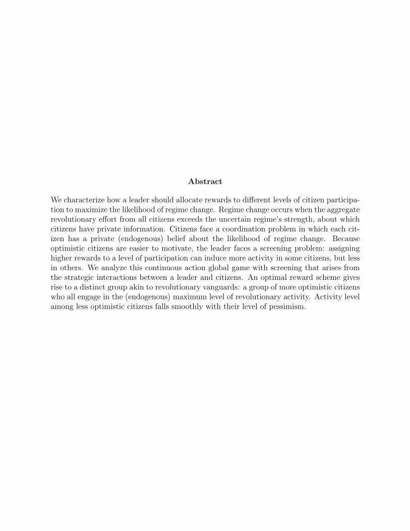
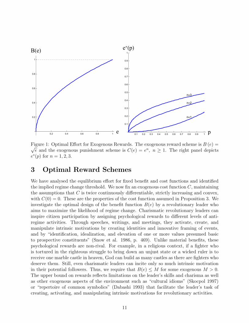
We conclude this section by reporting a class of examples. Suppose that the exogenousreward scheme is B (e) =

√e and the punishment scheme is C(e) = en, n ≥ 1. In this

case, we have from Proposition 3 that e∗(p) = ( p2n

)2

2n−1 and

θe∗ =2n− 1

2n+ 1(2n)

21−2n .

Figure 1 illustrates.

10

0.2 0.4 0.6 0.8 1 e

0.2

0.4

0.6

0.8

1

B(e)

n=1

n=2

n=3

0.1 0.2 0.3 0.4 0.5 0.6 0.7 0.8 0.9 1 p

0.1

0.2

0.3

0.4

0.5

0.6

0.7

0.8

0.9

1

e*(p)

Figure 1: Optimal Effort for Exogenous Rewards. The exogenous reward scheme is B (e) =√e and the exogenous punishment scheme is C(e) = en, n ≥ 1. The right panel depicts

e∗(p) for n = 1, 2, 3.

3 Optimal Reward Schemes

We have analysed the equilibrium effort for fixed benefit and cost functions and identifiedthe implied regime change threshold. We now fix an exogenous cost function C, maintainingthe assumptions that C is twice continuously differentiable, strictly increasing and convex,with C(0) = 0. These are the properties of the cost function assumed in Proposition 3. Weinvestigate the optimal design of the benefit function B(e) by a revolutionary leader whoaims to maximize the likelihood of regime change. Charismatic revolutionary leaders caninspire citizen participation by assigning psychological rewards to different levels of anti-regime activities. Through speeches, writings, and meetings, they activate, create, andmanipulate intrinsic motivations by creating identities and innovative framing of events,and by “identification, idealization, and elevation of one or more values presumed basicto prospective constituents” (Snow et al. 1986, p. 469). Unlike material benefits, thesepsychological rewards are non-rival. For example, in a religious context, if a fighter whois tortured in the righteous struggle to bring down an unjust state or a wicked ruler is toreceive one marble castle in heaven, God can build as many castles as there are fighters whodeserve them. Still, even charismatic leaders can incite only so much intrinsic motivationin their potential followers. Thus, we require that B(e) ≤ M for some exogenous M > 0.The upper bound on rewards reflects limitations on the leader’s skills and charisma as wellas other exogenous aspects of the environment such as “cultural idioms” (Skocpol 1997)or “repertoire of common symbolics” (Dabashi 1993) that facilitate the leader’s task ofcreating, activating, and manipulating intrinsic motivations for revolutionary activities.

11

Proposition 2 implies that e∗(p) is weakly increasing (recall that this proposition didnot impose any assumptions on the benefit function). By Proposition 2, we then knowthat—for any choice of B (·)—there will be a unique equilibrium in which regime change

occurs when θ ≤ θe∗ =´ 1

p=0e∗(p)dp. Thus the leader’s optimization problem reduces to

choosing reward scheme B(e) to maximize the regime change threshold

ˆ 1

p=0

e∗(p)dp (8)

subject to the optimality of the effort function

e∗(p) ∈ arg maxe≥0

p B(e)− C(e),

and the feasibility of the reward scheme

B(e) ∈ [0,M ] for all e. (9)

A reward scheme B∗ that maximizes this problem is an optimal reward scheme (therewill be some indeterminacy in optimal reward schemes). An effort function e∗ arising inthis problem is an optimal effort function (there will be an essentially unique optimal effortfunction). The regime change threshold θ∗ that results from the optimal effort functionis the (essentially unique) optimal regime change threshold. To provide intuition and asa benchmark, we first present the analysis with linear costs, and then present our mainresult.

3.1 Linear Costs

Proposition 4. Suppose costs are linear, with constant marginal cost c. An optimal rewardscheme B∗ is the step function

B∗(e) =

{0 ; e < M/2c

M ; e ≥M/2c.(10)

The optimal effort function e∗ is the step function

e∗(p) =

{0 ; p < 1/2

M/2c ; p ≥ 1/2.(11)

And the optimal regime change threshold is

θe∗ = M/4c.

Any reward scheme giving rise to the optimal effort function is optimal. Thus, it isenough, for example, that B∗(0) = 0, B∗(M/2c) = M and B∗(e) ≤ 2ce for e ≤M/2c.

12

To prove the proposition, first assume the optimal reward scheme is a step function,where citizens get the maximum benefit M if they exert at least effort e; otherwise they getno benefit. In this case, citizens either do not participate (i.e., choose effort 0) or partici-pate with effort e. A citizen with optimism (probability of regime change) p participateswhenever pM ≥ ce, i.e., p ≥ ce/M . Thus, the total effort is (1− ce/M) e. This is maxi-mized by setting e = M/2c. Thus we have a proof of the proposition if we could establishthat the optimal reward schemes would be a step function.

To complete the proof, we show we can restrict attention to step functions. To dothis, we show that this problem reduces to the monopoly pricing problem. Consider amonopolist selling a single unit to buyers whose valuations are uniformly distributed onthe interval [0,M/c]. The monopolist could sell using a posted price mechanism. At aposted price of e, buyers with valuations above e would buy and pay e, and buyers withvaluations below e would not buy. However, the monopolist could also sell using a morecomplicated mechanism, offering a price schedule for probabilities of being allocated theobject. By the revelation principle, we can restrict attention to direct mechanisms. Ifa type-p buyer has valuation pM/c, a direct mechanism is described by a payment e∗(p)that buyer p will make to the seller and a probability B (e∗(p)) /M of receiving the object.

The seller’s revenue will now be´ 1

p=0e∗(p)dp and incentive compatibility will require that

e∗(p)∈ arg maxe≥0 p B(e)/c − e. The revenue is the maximand of our problem and theincentive compatibility condition is the incentive compatibility condition of our problem.But Riley and Zackhauser (1983) established that the optimal mechanism in this problemis a posted price mechanism (see Borgers (2015, Ch. 2) for a modern textbook treatment),and simple calculations show that the optimal price is M/2c. This proves Proposition 4.

Our main result establishes that if the cost function is strictly convex, this step functionis “smoothed”: it remains optimal for a mass of the most optimistic citizens to choose amaximum effort level and receive the maximum reward. And it remains optimal (undersome conditions) for a mass of the least optimistic citizens to not participate, i.e., choose0 and receive no benefit. However, in between there are strictly increasing benefits andeffort.

We conclude our analysis of the linear case by discussing why bunching at the top startsexactly when p = 1/2. Recall that our strategic problem delivers a particular distributionover levels of optimism p: the uniform distribution. In the monopoly problem, this isequivalent to considering a linear demand curve. It is useful to consider what would havehappened in the screening problem if p was not uniformly distributed, but distributedaccording to density f and corresponding cdf F . Under standard assumptions,3 the problemreduces to solving for the critical effort level e to receive the (maximum) benefit. As before,the citizen will participate at this critical effort level if p ≥ ce/M . But now total effortwould be (1− F (ce/M)) e. Letting e∗ be the optimal e, the first order condition implies

e∗ =1− F (ce∗/M)

f (ce∗/M)

M

c,

3In particular, f should satisfy the standard regularity condition that 1−F (·)f(·) is decreasing (decreasing

marginal revenue in the monopoly case).

13

and the corresponding critical optimism level is

p∗ = ce∗/M =1− F (ce∗/M)

f (ce∗/M).

When p is distributed uniformly, the above equation implies that ce∗/M = 1/2. Thus,p∗ = 1/2 arises as critical optimism because p is uniformly distributed.

3.2 Strictly Convex Costs and Main Result

Proposition 5. Suppose costs are strictly convex.

• For some “maximum effort” e > 0, the optimal reward scheme is continuous, strictlyincreasing and strictly convex on the interval [0, e] with B (0) = 0 and B (e) = M .Moreover, the marginal benefit of effort B′(e) is strictly greater than the marginalcost of effort C ′ (e) whenever the marginal benefit is non-zero

• The optimal effort function is continuous and weakly increasing; it is strictly increas-ing on an interval

[p, 1/2

], equal to 0 when p ≤ p, and equal to e when p ≥ 1/2.

• The critical level of optimism p is strictly greater than 0 if and only if the marginalcost is strictly positive at zero effort (C ′(0) > 0).

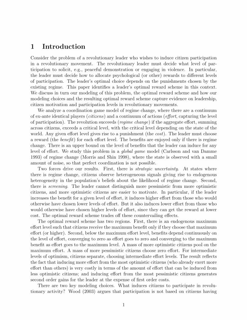
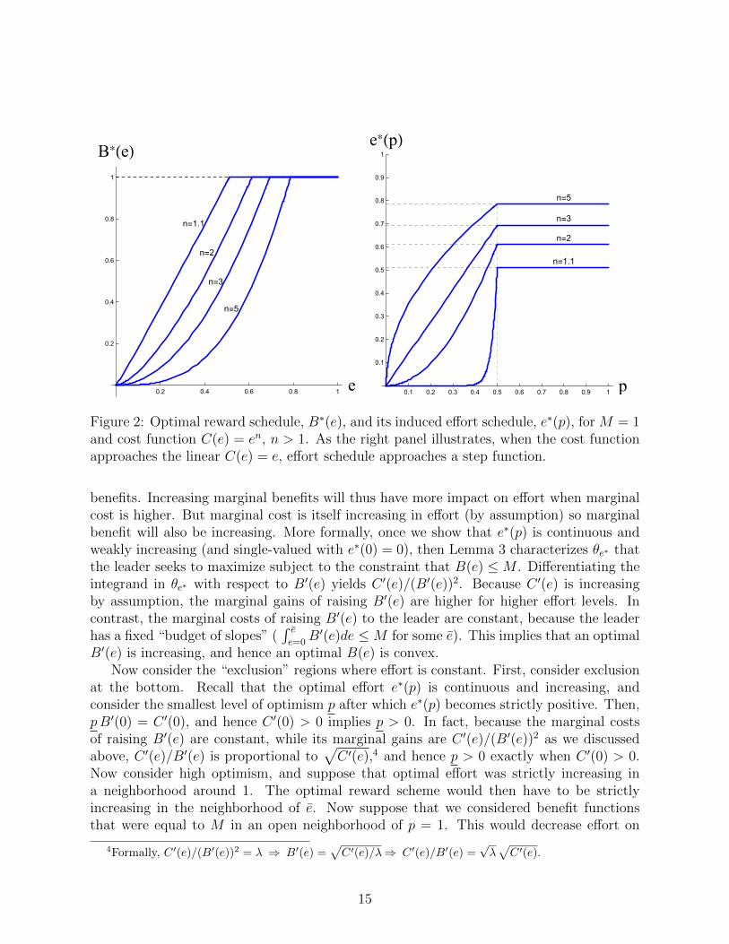
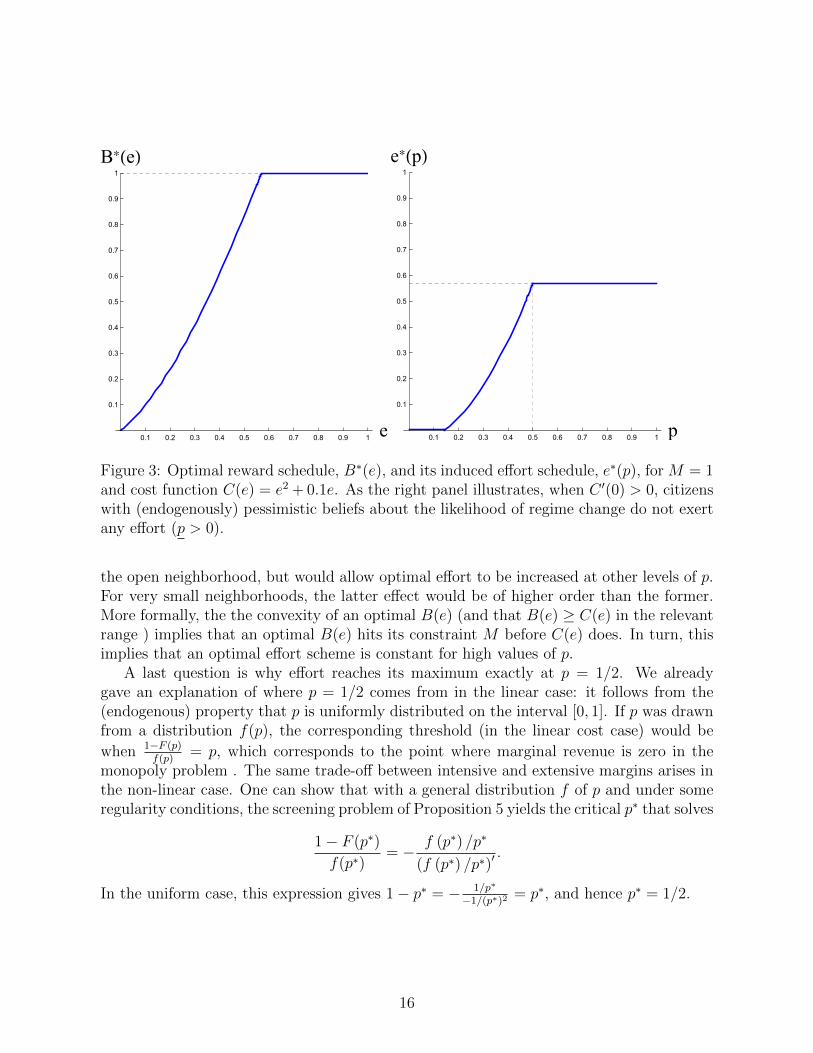
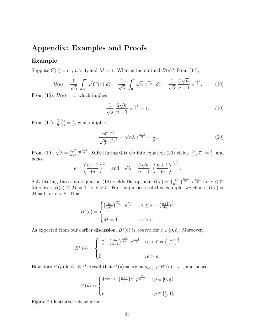
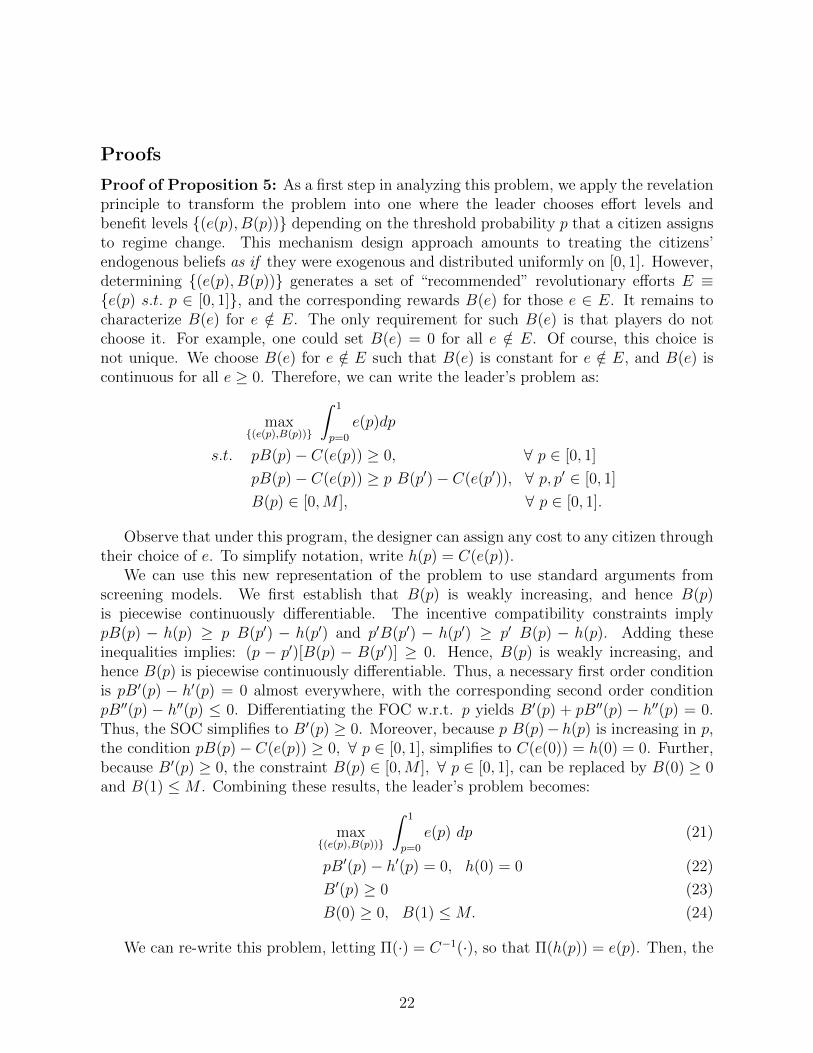
To illustrate the proposition, we graph the optimal reward scheme and optimal effort func-tion for some examples. First, suppose C(e) = en, n > 1, and M = 1. Figure 2 illustratesthe optimal reward and optimal effort schemes in this case for different values of n. Thederivation is reported in the appendix. Note that as n approaches 1, we approach thelinear case described above (as noted earlier, there is an indeterminacy in the optimal re-ward scheme, and this limit is piece-wise linear, rather than the step function reportedin Proposition 4). This class of examples has C ′(0) = 0. Figure 3 illustrates an examplewhere C(e) = e2 + 0.1e, so that the marginal cost at 0 is strictly positive, C ′(0) = 0.1.

Further details about the optimal reward scheme and the optimal effort function, as wellas an algorithm for calculating them, are reported below in the proof of the proposition.

The basic features of the optimal reward scheme and optimal effort function are intu-itive: both are weakly increasing and continuous, with optimal benefit strictly increasingand ranging from 0 to the maximum. Before presenting a proof, we provide an intuitionfor further properties. First, consider the shape of the optimal reward scheme when it isstrictly increasing. In this case, marginal benefit exceeds the marginal cost. If the marginalcost did exceed the marginal benefit at some effort level, then any effort in the neighbor-hood of that level could not arise in equilibrium. But then it would be possible to replacethe reward scheme with one that was constant in that neighborhood and increasing fasterelsewhere, in a way that would increase the overall effort. More mechanically, the first ordercondition that pB′(e∗(p)) = C ′(e∗(p)) implies that B′(e∗(p)) > C ′(e∗(p)) when p < 1. Toshow strict convexity, observe that effort depends on the ratio of marginal costs to marginal

14

n=1.1

n=2

n=3

n=5

0.2 0.4 0.6 0.8 1 e

0.2

0.4

0.6

0.8

1

B*(e)

n=1.1

n=2

n=3

n=5

0.1 0.2 0.3 0.4 0.5 0.6 0.7 0.8 0.9 1 p

0.1

0.2

0.3

0.4

0.5

0.6

0.7

0.8

0.9

1

e*(p)

Figure 2: Optimal reward schedule, B∗(e), and its induced effort schedule, e∗(p), for M = 1and cost function C(e) = en, n > 1. As the right panel illustrates, when the cost functionapproaches the linear C(e) = e, effort schedule approaches a step function.

benefits. Increasing marginal benefits will thus have more impact on effort when marginalcost is higher. But marginal cost is itself increasing in effort (by assumption) so marginalbenefit will also be increasing. More formally, once we show that e∗(p) is continuous andweakly increasing (and single-valued with e∗(0) = 0), then Lemma 3 characterizes θe∗ thatthe leader seeks to maximize subject to the constraint that B(e) ≤M . Differentiating theintegrand in θe∗ with respect to B′(e) yields C ′(e)/(B′(e))2. Because C ′(e) is increasingby assumption, the marginal gains of raising B′(e) are higher for higher effort levels. Incontrast, the marginal costs of raising B′(e) to the leader are constant, because the leaderhas a fixed “budget of slopes” (

´ ee=0

B′(e)de ≤M for some e). This implies that an optimalB′(e) is increasing, and hence an optimal B(e) is convex.

Now consider the “exclusion” regions where effort is constant. First, consider exclusionat the bottom. Recall that the optimal effort e∗(p) is continuous and increasing, andconsider the smallest level of optimism p after which e∗(p) becomes strictly positive. Then,pB′(0) = C ′(0), and hence C ′(0) > 0 implies p > 0. In fact, because the marginal costsof raising B′(e) are constant, while its marginal gains are C ′(e)/(B′(e))2 as we discussedabove, C ′(e)/B′(e) is proportional to

√C ′(e),4 and hence p > 0 exactly when C ′(0) > 0.

Now consider high optimism, and suppose that optimal effort was strictly increasing ina neighborhood around 1. The optimal reward scheme would then have to be strictlyincreasing in the neighborhood of e. Now suppose that we considered benefit functionsthat were equal to M in an open neighborhood of p = 1. This would decrease effort on

4Formally, C ′(e)/(B′(e))2 = λ ⇒ B′(e) =√C ′(e)/λ⇒ C ′(e)/B′(e) =

√λ√C ′(e).

15

0.1 0.2 0.3 0.4 0.5 0.6 0.7 0.8 0.9 1 e

0.1

0.2

0.3

0.4

0.5

0.6

0.7

0.8

0.9

1

B*(e)

0.1 0.2 0.3 0.4 0.5 0.6 0.7 0.8 0.9 1 p

0.1

0.2

0.3

0.4

0.5

0.6

0.7

0.8

0.9

1

e*(p)

Figure 3: Optimal reward schedule, B∗(e), and its induced effort schedule, e∗(p), for M = 1and cost function C(e) = e2 + 0.1e. As the right panel illustrates, when C ′(0) > 0, citizenswith (endogenously) pessimistic beliefs about the likelihood of regime change do not exertany effort (p > 0).

the open neighborhood, but would allow optimal effort to be increased at other levels of p.For very small neighborhoods, the latter effect would be of higher order than the former.More formally, the the convexity of an optimal B(e) (and that B(e) ≥ C(e) in the relevantrange ) implies that an optimal B(e) hits its constraint M before C(e) does. In turn, thisimplies that an optimal effort scheme is constant for high values of p.

A last question is why effort reaches its maximum exactly at p = 1/2. We alreadygave an explanation of where p = 1/2 comes from in the linear case: it follows from the(endogenous) property that p is uniformly distributed on the interval [0, 1]. If p was drawnfrom a distribution f(p), the corresponding threshold (in the linear cost case) would be

when 1−F (p)f(p)

= p, which corresponds to the point where marginal revenue is zero in themonopoly problem . The same trade-off between intensive and extensive margins arises inthe non-linear case. One can show that with a general distribution f of p and under someregularity conditions, the screening problem of Proposition 5 yields the critical p∗ that solves

1− F (p∗)

f(p∗)= − f (p∗) /p∗

(f (p∗) /p∗)′.

In the uniform case, this expression gives 1− p∗ = − 1/p∗

−1/(p∗)2= p∗, and hence p∗ = 1/2.

16

3.3 Proof

We now present the proof of Proposition 5, formalizing the earlier intuitions. We defermore technical steps to the appendix, where we formalize the leader’s problem as a mech-anism design problem, and prove that an optimal reward function e∗(p) is continuous andincreasing with e∗(0) = 0. Then, using Lemma 3, we show that the leader’s problem is tochoose (e, B′) to maximize

ˆ e

0

(1− C ′(e)

B′(e)

)de

subject to the marginal benefit constraint that5

B (e) =

ˆ e

e=0

B′(e)de = M.

This shows that one can think of the leader’s problem as him deciding a maximum level ofeffort e ≥ 0 to induce, and then deciding how to allocate a fixed supply of marginal benefitto different effort levels B′ : [0, e]→ R.

Thus, the leader’s problem becomes a constrained point-wise optimization. The La-grangian is

L =

ˆ e

0

(1− C ′(e)

B′(e)

)de+ λ

(M −

ˆ e

e=0

B′(e)de

)=

ˆ e

0

(1− C ′(e)

B′(e)− λ B′(e)

)de+ λ M.

Optimal B′(e) simplifies to a point-wise maximization

∂L

∂B′(e)

(1− C ′(e)

B′(e)− λ B′(e)

)=

C ′(e)

[B′(e)]2− λ = 0. (12)

This shows that at the optimum, the marginal gain of raising B′(e), i.e., C ′(e)/[B′(e)]2,equals its marginal cost λ. Thus,

B′(x) =1√λ

√C ′(x), (13)

and

B(e) =

ˆ e

0

B′(x)dx =1√λ

ˆ e

0

√C ′(x) dx. (14)

5There are two other constraints: e ≥ 0 and B′(e) ≥ C ′(e). However, as it will be clear from thesolution, these two constraints are automatically satisfied.

17

Combining this with the constraint yields

B(e) =1√λ

ˆ e

0

√C ′(x) dx = M. (15)

Moreover, optimal e also satisfies the first order condition

∂L

∂e= 1− C ′(e)

B′(e)− λ B′(e) = 0 ⇒ 1− C ′(e)

B′(e)= λ B′(e). (16)

Substituting for λ from (12) into (16) yields

1− C ′(e)

B′(e)=C ′(e)

B′(e)⇒ C ′(e)

B′(e)=

1

2. (17)

So if e and λ are the solution to equations (15) and (17), we have solved for B.

From equation (13), we have C′(e)B′(e)

=√λC ′(e) > 0. This has two implications: (1)

because C(e) is strictly convex, B(e) is strictly convex for 0 < e < e; and C′(e)B′(e)

is strictly

increasing. Thus, C′(e)B′(e)

= 12

implies that B′(e) ≥ C ′(e). (2) e∗(p) is strictly increasing

between p =√λ√C ′(0) and p = 1/2; it is equal to 0 for p ≤ p and equal to e for p ≥ 1/2.

4 Discussion: Inspiring Revolutionary Activities

4.1 Pleasure in Agency

What motivates citizens to participate in revolutions, civil wars, or other anti-regime collec-tive actions, where individual effects are minimal, risks are high, and the fruits of successare public? This question is the essence of Tullock’s (1971) “Paradox of Revolution,”which specialized Olson’s (1965) Logic of Collective Action to revolution settings. Onepossible answer is that participants somehow receive selective material rewards. However,as Blattman and Miguel (2010) argue in their review of the civil war literature, even insuch risky environments, “non-material incentives are thought to be common [even] withinarmed groups. Several studies argue that a leader’s charisma, group ideology, or a citizen’ssatisfaction in pursuit of justice (or vengeance) can also help solve the problem of collectiveaction in rebellion” (p. 15). Similarly, in the broader context of protests and revolutions,researchers have persistently pointed to the critical role of non-material incentives amongthe participants. For example, based partly on his field work in Eastern Europe, Petersen(2001) argues that non-material status rewards and the feelings of self-respect were essentialcomponents of the insurgents’ motives; and Pearlman (2016) highlights the role of “moralidentity” (e.g., self-respect and “joy of agency”) in Syrian protests.

What exactly is the nature of these non-material incentives? In this paper, we focuson the notion of “pleasure in agency.” Wood (2003) develops the notion of “pleasure inagency” to capture individuals’ motives for participating in contentious collective actions.

18

Pleasure in agency is “the positive effect associated with self-determination, autonomy, self-esteem, efficacy, and pride that come from the successful assertion of intention” (p. 235).It is “a frequency-based motivation: it depends on the likelihood of success, which in turnincreases with the number participating (Schelling 1978; Hardin 1982). Yet the pleasure inagency is undiminished by the fact that one’s own contribution to the likelihood of victoryis vanishingly small” (p. 235-6). For example, in her interviews with insurgents duringand after the El Salvadoran civil war, she found that insurgents “repeatedly asserted theirpride in their wartime activities and consistently claimed authorship of the changes thatthey identified as their work” (p. 231). “They took pride, indeed pleasure, in the successfulassertion of their interests and identity...motivated in part by the value they put on beingpart of the making of history” (p. 18-9).

4.2 The Role of Leaders

Although many scholars agree that “an account of participation in insurgency requires aconsideration of the moral and emotional dimensions of participation” (Wood 2003, p. 225),they typically consider these intrinsic motivations as the natural and automatic result ofpast experiences or the interactions with the regime in periods of contention. We argue thatleaders can maximize the likelihood of regime change by strategically creating, activating,or manipulating such feelings and emotions to design an optimal scheme of “pleasure inagency” as the function of citizens’ level of anti-regime activities.

In his review of the literature on revolutions, Goldstone (2001) identifies two distincttypes of revolutionary leaders: people-oriented and task-oriented. “People-oriented leadersare those who inspire people, give them a sense of identity and power, and provide a visionof a new and just order” (p. 157). These are leaders who can create, amplify, or transformpeople’s feelings and identities, e.g., by innovative framing of events and experiences andtheir personality traits such as their charisma (Snow et al. 1986). In the terminologyof the management science organizational behavior, they are “transformational leaders”who have the ability to create inspirational motivations through a variety of psychologicalmechanisms (Burns 1978, 2003; Bass 1985). In contrast to people-oriented leaders, in Gold-stone (2001), “task-oriented leaders are those who can plot a strategy suitable to resourcesand circumstances” (p. 157), including the repressive capacity of the state and availablerevolutionary skills, to effectively transform anti-regime sentiments into concrete actions.Combining these separate branches of the literature, we show how a“people-oriented” leadercan optimally create and manipulate “pleasure in agency” feelings among potential revo-lutionaries to maximize the likelihood of regime change. That even the design of optimal“pleasure in agency schemes” requires “a strategy suitable to resources and circumstances”merges the seemingly separate categories of people-oriented and task-oriented leadership.

4.3 Levels of Participation

Charles Tilly defines Contentious Performances (Tilly 2008) to be political, collective claim-making actions that fall outside routine social interactions. Such contentious actions take

19

various forms. Examples include machine-breaking, petitioning, arson (e.g., common inthe Swing Rebellion), cattle maiming (e.g., in Tithe War in Ireland), sit-ins in foreignembassies (e.g., in the 1905-07 Iranian Constitutional Revolution), noise-making throughcacerolazo (banging on pots and pans, e.g., in 1989 Caracazo in Venezuela), shouting slogansfrom the roof tops at night (e.g., in the 1979 Iranian Revolution), occupation of a publicspace or a government building, writing open letters, wearing a particular color (e.g., greenwristbands in the 2009 Iranian green movement, orange ribbons in the Ukrainian OrangeRevolution, or yellow ribbons in the Yellow Revolution in the Philippines), public meetings,boycotts (e.g., in the American Revolution), parades (e.g., women suffrage movement inthe early 20th century), strikes, marches, demonstrations, freedom rides, street blockades,self-immolation, suicide bombing, assassination, hijacking, and guerrilla war.

Some contentious actions require more effort and taking more risks than others. For ex-ample, taking up arms against a regime takes far more effort and is far more dangerous thanparticipating in a demonstration, which in turn is typically more costly than participating ina boycott campaign (Shadmehr 2015). That is, different levels of anti-regime activities cor-respond to different contentious performances. Our analysis shows how a “people-oriented”revolutionary leader, for a given repression structure, C(e), should strategically create andmanipulate pleasure in agency, B(e), that citizens obtain from different contentious perfor-mances, e, to maximize the likelihood of regime change.

4.4 Professional Revolutionaries

Our main result (Proposition 5) implies that, no matter what the leader’s ability M , theleader’s optimal design of (pleasure in agency) rewards leads to the emergence of a group ofcitizens who engage in maximum level of anti-regime activities. The creation of this “cadre”is consistent with the notion of professional revolutionaries in Lenin’s treatise, What Is tobe Done? 6 Although this group is distinct from other citizens contributing to the cause,there is little difference among the magnitude of duties and the levels of revolutionaryactivities among the members of the group. Contrasting the organization of workers, whoengage in various degrees of contentious activities, with the organization of “revolutionarysocial-democratic party,” Lenin insisted that “the organization of the revolutionaries mustconsist first and foremost of people who make revolutionary activity their profession.... Inview of this common characteristic of the members of such an organization, all distinctionsas between workers and intellectuals, not to speak of distinctions of trade and profession,in both categories, must be effaced” (p. 71). Of course, the members of this group are notidentical; some have stronger beliefs in the likelihood of regime change p than others, forexample, as a result of their different interpretations of Marxist theory, or differences inmapping from the real world into the theory. However, despite these differences in theirbeliefs, they constitute a distinct group that exert maximum effort into the revolution—inthis sense, they are professional revolutionaries.

6It also resonates with the notion of “combat groups” in Mao’s On Guerrilla Warfare.

20

Appendix: Examples and Proofs

Example

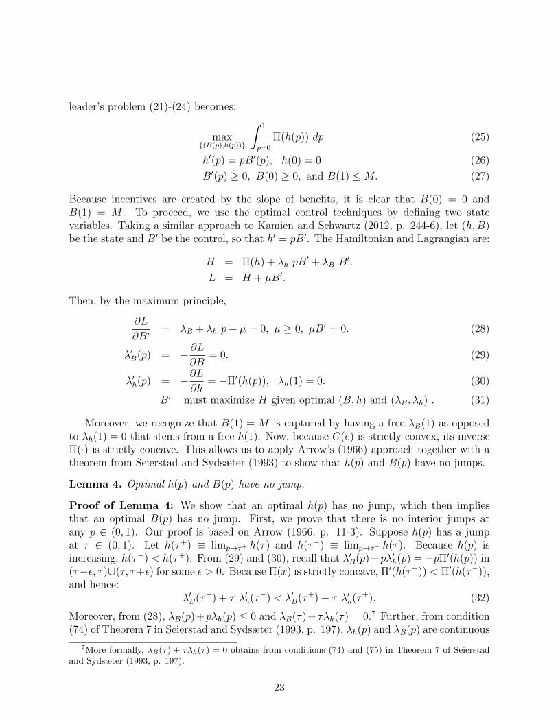
Suppose C(e) = en, n > 1, and M = 1. What is the optimal B(e)? From (14),

B(e) =1√λ

ˆ e

0

√C ′(x) dx =

1√λ

ˆ e

0

√n x

n−12 dx =

1√λ

2√n

n+ 1e

n+12 . (18)

From (15), B(e) = 1, which implies

1√λ

2√n

n+ 1e

n+12 = 1. (19)

From (17), C′(e)B′(e)

= 12, which implies

nen−1√nλe

n−12

=√nλ e

n−12 =

1

2. (20)

From (19),√λ = 2

√n

n+1e

n+12 . Substituting this

√λ into equation (20) yields 2n

n+1en = 1

2, and

hence

e =

(n+ 1

4n

) 1n

and√λ =

2√n

n+ 1

(n+ 1

4n

)n+12n

.

Substituting these into equation (18) yields the optimal B(e) =(

4nn+1

)n+12n e

n+12 for e ≤ e.

Moreover, B(e) ≤ M = 1 for e > e. For the purposes of this example, we choose B(e) =M = 1 for e > e. Thus,

B∗(e) =

(

4nn+1

)n+12n e

n+12 ; e ≤ e =

(n+14n

) 1n

M = 1 ; e > e.

As expected from our earlier discussion, B∗(e) is convex for e ∈ [0, e]. Moreover,

B∗′(e) =

n+1

2

(4nn+1

)n+12n e

n−12 ; e < e =

(n+14n

) 1n

0 ; e > e.

How does e∗(p) look like? Recall that e∗(p) = arg maxe≥0 p B∗(e)− en, and hence

e∗(p) =

4

1n(n−1)

(n+1n

) 1n p

2n−1 ; p ∈ [0, 1

2)

e ; p ∈ [12, 1].

Figure 2 illustrated this solution.

21

Proofs

Proof of Proposition 5: As a first step in analyzing this problem, we apply the revelationprinciple to transform the problem into one where the leader chooses effort levels andbenefit levels {(e(p), B(p))} depending on the threshold probability p that a citizen assignsto regime change. This mechanism design approach amounts to treating the citizens’endogenous beliefs as if they were exogenous and distributed uniformly on [0, 1]. However,determining {(e(p), B(p))} generates a set of “recommended” revolutionary efforts E ≡{e(p) s.t. p ∈ [0, 1]}, and the corresponding rewards B(e) for those e ∈ E. It remains tocharacterize B(e) for e /∈ E. The only requirement for such B(e) is that players do notchoose it. For example, one could set B(e) = 0 for all e /∈ E. Of course, this choice isnot unique. We choose B(e) for e /∈ E such that B(e) is constant for e /∈ E, and B(e) iscontinuous for all e ≥ 0. Therefore, we can write the leader’s problem as:

max{(e(p),B(p))}

ˆ 1

p=0

e(p)dp

s.t. pB(p)− C(e(p)) ≥ 0, ∀ p ∈ [0, 1]

pB(p)− C(e(p)) ≥ p B(p′)− C(e(p′)), ∀ p, p′ ∈ [0, 1]

B(p) ∈ [0,M ], ∀ p ∈ [0, 1].

Observe that under this program, the designer can assign any cost to any citizen throughtheir choice of e. To simplify notation, write h(p) = C(e(p)).

We can use this new representation of the problem to use standard arguments fromscreening models. We first establish that B(p) is weakly increasing, and hence B(p)is piecewise continuously differentiable. The incentive compatibility constraints implypB(p) − h(p) ≥ p B(p′) − h(p′) and p′B(p′) − h(p′) ≥ p′ B(p) − h(p). Adding theseinequalities implies: (p − p′)[B(p) − B(p′)] ≥ 0. Hence, B(p) is weakly increasing, andhence B(p) is piecewise continuously differentiable. Thus, a necessary first order conditionis pB′(p) − h′(p) = 0 almost everywhere, with the corresponding second order conditionpB′′(p) − h′′(p) ≤ 0. Differentiating the FOC w.r.t. p yields B′(p) + pB′′(p) − h′′(p) = 0.Thus, the SOC simplifies to B′(p) ≥ 0. Moreover, because p B(p)− h(p) is increasing in p,the condition pB(p)− C(e(p)) ≥ 0, ∀ p ∈ [0, 1], simplifies to C(e(0)) = h(0) = 0. Further,because B′(p) ≥ 0, the constraint B(p) ∈ [0,M ], ∀ p ∈ [0, 1], can be replaced by B(0) ≥ 0and B(1) ≤M . Combining these results, the leader’s problem becomes:

max{(e(p),B(p))}

ˆ 1

p=0

e(p) dp (21)

pB′(p)− h′(p) = 0, h(0) = 0 (22)

B′(p) ≥ 0 (23)

B(0) ≥ 0, B(1) ≤M. (24)

We can re-write this problem, letting Π(·) = C−1(·), so that Π(h(p)) = e(p). Then, the

22

leader’s problem (21)-(24) becomes:

max{(B(p),h(p))}

ˆ 1

p=0

Π(h(p)) dp (25)

h′(p) = pB′(p), h(0) = 0 (26)

B′(p) ≥ 0, B(0) ≥ 0, and B(1) ≤M. (27)

Because incentives are created by the slope of benefits, it is clear that B(0) = 0 andB(1) = M . To proceed, we use the optimal control techniques by defining two statevariables. Taking a similar approach to Kamien and Schwartz (2012, p. 244-6), let (h,B)be the state and B′ be the control, so that h′ = pB′. The Hamiltonian and Lagrangian are:

H = Π(h) + λh pB′ + λB B′.

L = H + µB′.

Then, by the maximum principle,

∂L

∂B′= λB + λh p+ µ = 0, µ ≥ 0, µB′ = 0. (28)

λ′B(p) = − ∂L∂B

= 0. (29)

λ′h(p) = −∂L∂h

= −Π′(h(p)), λh(1) = 0. (30)

B′ must maximize H given optimal (B, h) and (λB, λh) . (31)

Moreover, we recognize that B(1) = M is captured by having a free λB(1) as opposedto λh(1) = 0 that stems from a free h(1). Now, because C(e) is strictly convex, its inverseΠ(·) is strictly concave. This allows us to apply Arrow’s (1966) approach together with atheorem from Seierstad and Sydsæter (1993) to show that h(p) and B(p) have no jumps.

Lemma 4. Optimal h(p) and B(p) have no jump.

Proof of Lemma 4: We show that an optimal h(p) has no jump, which then impliesthat an optimal B(p) has no jump. First, we prove that there is no interior jumps atany p ∈ (0, 1). Our proof is based on Arrow (1966, p. 11-3). Suppose h(p) has a jumpat τ ∈ (0, 1). Let h(τ+) ≡ limp→τ+ h(τ) and h(τ−) ≡ limp→τ− h(τ). Because h(p) isincreasing, h(τ−) < h(τ+). From (29) and (30), recall that λ′B(p)+pλ′h(p) = −pΠ′(h(p)) in(τ−ε, τ)∪(τ, τ+ε) for some ε > 0. Because Π(x) is strictly concave, Π′(h(τ+)) < Π′(h(τ−)),and hence:

λ′B(τ−) + τ λ′h(τ−) < λ′B(τ+) + τ λ′h(τ

+). (32)

Moreover, from (28), λB(p)+pλh(p) ≤ 0 and λB(τ)+ τλh(τ) = 0.7 Further, from condition(74) of Theorem 7 in Seierstad and Sydsæter (1993, p. 197), λh(p) and λB(p) are continuous

7More formally, λB(τ) + τλh(τ) = 0 obtains from conditions (74) and (75) in Theorem 7 of Seierstadand Sydsæter (1993, p. 197).

23

at τ . Thus, in a right neighborhood of τ , we have λ′B(p) + pλ′h(p) +λh(p) ≤ 0, and in a leftneighborhood of τ , we have λ′B(p) + pλ′h(p) + λh(p) ≥ 0. But this contradicts (32).

Next, we prove that there is no jump at p = 0 or p = 1. From (29), λB(p) = constant ≡λ on p ∈ (0, 1). Moreover, λB(p) is continuous (Seierstad and Sydsæter 1993, p. 197).Thus, λB(p) = λ, for p ∈ [0, 1]. From conditions (74) and (75) in Theorem 7 of Seierstadand Sydsæter (1993, p. 197), λB(τ) + τλh(τ) = 0. Combining this with λB(p) = λ and

(30), λ + τ´ 1

x=τΠ′(h(x))dx = 0. In particular, if τ = 0 or τ = 1, then λ = 0. But from

(28), λ+λh p ≤ 0 and λh(p) =´ 1

x=pΠ′(h(x))dx is positive for some p ∈ (0, 1). Thus, λ < 0.

A contradiction. �

From (29) and (30),

λB(p) = constant = λ and λh(p) = −ˆ 1

x=p

λ′h(x)dx =

ˆ 1

x=p

Π′(h(x))dx. (33)

Moreover, from (28), λ+ p λh(p) ≤ 0. Because at p ∈ (0, 1), p λh(p) = p´ 1

x=pΠ′(h(x))dx >

0, we must have λ < 0.

Lemma 5. There is no interior bunching. That is, there is no 0 < p1 < p2 < 1 suchthat h′(p) = 0 for p ∈ (p1, p2), with h′(p) > 0 in a left neighborhood of p1 and in a rightneighborhood of p2 .

Proof of Lemma 5: Suppose not. Let h(p) = h for p ∈ [p1, p2]. Because h(p) and henceB(p) must be strictly increasing in a left neighborhood of p1 and in a right neighborhoodof p2, µ = 0 in those neighborhoods. Moreover, λB(p) and λh(p) are continuous. Therefore,(28) implies that λB(p1)+p1λh(p1) = 0 = λB(p2)+p2λh(p2). Because λB(p) = λ from (33),we have,

p1λh(p1) = p2λh(p2). (34)

Further, from (33),

λh(p1) =

ˆ p2

p1

Π′(h(x))dx+

ˆ 1

p2

Π′(h(x))dx = (p2 − p1) Π′(h) + λh(p2). (35)

Combining equations (34) and (35) yields:

p1 Π′(h) = λh(p2). (36)

Next, consider p3 ∈ (p1, p2). From (28), λB(p3) + p3λh(p3) ≤ 0 = λB(p2) + p2λh(p2).Hence,

p3λh(p3) ≤ p2λh(p2). (37)

Mirroring the calculations of equation (35), we have:

λh(p3) = (p2 − p3) Π′(h) + λh(p2). (38)

24

Combining equations (37) and (38) yields:

p3 Π′(h) ≤ λh(p2). (39)

From equations (36) and (39), p3 Π′(h) ≤ p1 Π′(h). However, because p3 > p1 andΠ′(h) > 0, we must have p3 Π′(h) > p1 Π′(h), a contradiction. �

Next, we solve the problem ignoring the constraint B′(p) ≥ 0, and subsequently checkwhether and when this constraint binds. Without B′(p) ≥ 0, µ = 0, and hence from (28)and (33),

p

ˆ 1

x=p

Π′(h(x))dx+ λ = 0, and henced

dp

{p

ˆ 1

x=p

Π′(h(x))dx+ λ

}= 0 (40)

Differentiating (40) with respect to p yields Π′(h(p)) = − λp2

, and hence

h(p) = Π′−1

(− λp2

). (41)

Moreover, Because Π(h) is strictly concave, h(p) is strictly increasing, and hence B(p) isstrictly increasing as far as the constraints B(0) = 0 and B(1) = M are satisfied. Therefore,an optimal B(p) takes the following form:

B(p) =

0 ; p ∈ [0, p1]

strictly increasing function ; p ∈ [p1, p2]

M ; p ∈ [p2, 1],

for 0 ≤ p1 < p2 ≤ 1. This, in turn, implies a similar form for h(p), and hence for optimaleffort schedule:

e∗(p) =

0 ; p ∈ [0, p]

strictly increasing and satisfies the first order condition ; p ∈ [p, p]

e ; p ∈ [p, 1],

(42)

for some 0 ≤ p < p ≤ 1 and e > 0.Equation (42) together with Lemma 3 allows us to write the leader’s objective function

as:

θ∗ =

ˆ e

e=0

(1− C ′(e)

B′(e)

)de,

where we recognize that e∗(p) satisfying the first order condition implies B′(e) ≥ C ′(e),

and that p = C′(0)B′(0)

and p = C′(e)B′(e)

. Thus, we can formulate the leader’s problem as:

maxB′, e

ˆ e

0

(1− C ′(e)

B′(e)

)de

(43)

s.t. B(e) = M, B(0) = 0, B′(e) ≥ C ′(e), e ≥ 0,

25

Writing B(e) as B(e) =´ ee=0

B′(e)de, (43) can be written as:

maxB′, e

ˆ e

0

(1− C ′(e)

B′(e)

)de

s.t.

ˆ e

e=0

B′(e)de = M, B(0) = 0, B′(e) ≥ C ′(e), e ≥ 0.

This is the maximization problem that we analyze in Section 3.3 of the text. The rest ofthe proof is in the text. �

5 References

Arrow, Kenneth. 1966. “Optimal Capital Policy with Irreversible Investment.” Institutefor Mathematical Studies in Social Science, Stanford University.Baron, David, and Roger Myerson. 1982. “Regulating a Monopolist with Unknown Costs.”Econometrica 50 (4): 911-30.Bass, Bernard. 1985. Leadership and Performance Beyond Expectations. NY: Free Press.Blattman, Christopher, and Edward Miguel. 2010. “Civil War.” Journal of EconomicLiterature 48: 3-57.Borgers, Tilman. 2015. An Introduction to the Theory of Mechanism Design. New York:Oxford University Press.Bueno de Mesquita, Ethan. 2010. “Regime Change and Revolutionary Entrepreneurs.”AmericanPolitical Science Review 104 (3): 446-66.Burns, James MacGregor. 1978. Leadership. New York: Harper & Row Publishers.Burns, James MacGregor. 2003. Transforming Leadership: A New Pursuit of Happiness.New York: Grove Press.Chen, Heng, and Wing Suen. 2016. “Falling Dominoes: A Theory of Rare Events andCrisis Contagion.” American Economic Journal: Microeconomics 8: 1-29.Dabashi, Hamid. 1993. Theology of Discontent: The Ideological Foundation of the IslamicRevolution in Iran. New York: New York University Press.Edmond, Chris. 2013. “Information Manipulation, Coordination and Regime Change.”Review of Economic Studies 80: 1422-58.Egorov, Georgy, and Konstantin Sonin. 2017. “Elections in Non-Democracies.” Mimeo.Frankel, David, Ady Pauzner and Stephen Morris.2003. “Equilibrium Selection in GlobalGames with Strategic Complementarities,” Journal of Economic Theory 108: 1-44.Goldstone, Jack A. 2001. “Toward a Forth Generation of Revolutionary Theory.” AnnualReview of Political Science 4: 139-87.Guesnerie, Roger, and Jean-Jacques Laffont. 1984. “A Complete Solution to a Class ofPrincipal-Agent Problems with an Application in the Control of a Self-Managed Firm.”Journal of Public Economics 25: 329-69.Guimaraes, Bernardo, and Stephen Morris. 2007. “Risk and Wealth in a Model of Self-fulfilling Currency Attack.” Journal of Monetary Economics 54: 2205-30.

26

Hardin, Russell. 1982. Collective Action. Baltimore, MD: Johns Hopkins University Press.Hartline, Jason D. 2016. Mechanism Design and Approximation. Online Manuscript.Kamien, Morton, and Nancy Schwartz. 2012. Dynamic Optimization: The Calculus ofVariations and Optimal Control in Economics and Management (2nd Edition). Dover.Laffont, Jean-Jacques, and Jacques Robert. 1996. “Optimal Auction with FinanciallyConstrained Buyers.” Economics Letters 52: 181-86.Maskin, Eric, and John Riley. 1984. “Monopoly with Incomplete Information.” RANDJournal of Economics 15 (2): 171-96.Mookherjee, Dilip, and I. P. L. Png. 1994. “Marginal Deterrence in Enforcement of Law.”Journal of Political Economy 102 (5): 1039-66.Morris, Stephen, and Hyun Song Shin. 2003. “Global Games: Theory and Applica-tion.” In Advances in Economics and Econometrics, Theory and Applications, EighthWorld Congress, Volume I, edited by M. Dewatripont, L. P. Hansen, and S. J. Turnovsky.New York: Cambridge University Press.Mussa, Michael, and Sherwin Rosen. 1978. “Monopoly and Product Quality.” Journal ofEconomic Theory 18: 301-17.Olson, Mancur. 1965. The Logic of Collective Action: Public Goods and the Theory ofGroups. Cambridge, MA: Harvard University Press.Pearlman, Wendy. 2016. “Moral Identity and Protest Cascades in Syria.” British Journalof Political Science. Forthcoming.Petersen, Roger D. 2001. Resistance and Rebellion: Lessons from Eastern Europe. NewYork: Cambridge University Press.Quigley, Daniel, and Frederik Toscani. 2016. “The roles of transparency in regime change:Striking when the iron’s gone cold.” Mimeo.Riley, John, and Richard Zackhauser. 1983. “Optimal Selling Strategies: When to Haggle,When to Hold Firm.” Quarterly Journal of Economic 98 (2): 267-289.Schelling, Thomas C. 1978. Micromotives and Macrobehavior. New York: Norton.Seierstad, Atle, and Knut Sydsæter. 1993. Optimal Control Theory with Economic Appli-cations. Amsterdam, The Netherlands: Elsevier.Shadmehr, Mehdi. 2015. “Extremism in Revolutionary Movements.” Games and Eco-nomic Behavior 94: 97-121.Shadmehr, Mehdi. 2017. “Capitalists in Revolution.” Mimeo.Shen, Lin, and Junyuan Zou. 2016. “Intervention with Voluntary Participation in GlobalGames.” Mimeo.Skocpol, Theda. 1997. “Cultural Idioms and Political Ideologies in the RevolutionaryReconstruction of State Power: A Rejoinder to Sewell.” In Social Revolutions in the ModernWorld. Ed. by Theda Skocpol. New York: Cambridge University Press.Snow, David, Burke Rochford, Jr., Steven Worden, and Robert Benford. 1986. “BeliefAlignment Processes, Micromobilization, and Movement Participation.” American Socio-logical Review 51: 464-81.Tilly, Charles. 2008. Contentious Performances. New York: Cambridge University Press.Tullock, Gordon. 1971. “The Paradox of Revolution.” Public Choice 11: 89-99.

27

Tyson, Scott, and Alastair Smith. 2016. “Two-Sided Coordination: Competition in Col-lective Action.” Journal of Politics. Forthcoming.Wood, Elisabeth J. 2003. Insurgent Collective Action and Civil War in El Salvador. NewYork, NY: Cambridge University Press.

28