Revista de Geodezie, Cartografie ú i Cadastru Journal of ... · p p D t dp t t 1 ( ) ( 0) (2)...

Revista de Geodezie, Cartografie i Cadastru

Journal of Geodesy,

Cartography and Cadastre

Nr. 8

Bucure ti 2018

Journal of Geodesy, Cartography and Cadastre

2


3

Editorial Board

Prof. PhD. Habil. Eng. Ana-Cornelia BADEA - President Assoc. Prof. PhD. Eng. Adrian SAVU - Editor in chief

Headings coordinators: Assoc. Prof. PhD. Eng. Caius DIDULESCU Assoc. Prof. PhD. Eng. Octavian B DESCU PhD. Ioan STOIAN PhD. Vasile NACU

Editorial secretary Assist. Prof. PhD. Paul DUMITRU

Scientific Committee

Prof. PhD. Eng. Petre Iuliu DRAGOMIR

Prof. PhD. Eng. Dumitru ONOSE

Prof. PhD. Eng. Iohan NEUNER

Prof. PhD. Eng. Constantin CO ARC

Prof. PhD. Habil. Eng. Gheorghe BADEA

Prof. PhD. Eng. Maricel PALAMARIU

Prof. PhD. Habil. Eng. Carmen GRECEA

Prof. PhD. Eng. Cornel P UNESCU

Prof. PhD. Habil. Eng. Sorin HERBAN

Assoc. Prof. PhD. Eng. Livia NISTOR

Assoc. Prof. PhD. Eng. Constantin BOFU

Assoc. Prof. PhD. Eng. Constantin CHIRIL


4


5

Table of Contents

Table of Contents ....................................................................................................................................................... 5 Geo-gravimetric Quasi-geoid Determination over Romania Ileana Spiroiu, Radu-Dan-Nicolae Cri an, C t lin Erhan, Neculai Avramiuc, Milu Fluiera ................................ 6 Smart Managing Aeronautical Data Sabina Pl vicheanu, Florin Nache, Petre Iuliu Dragomir ................................................................................. 12 The use of VGI in noise mapping Efthimios Bakogiannis, Charalampos Kyriakidis, Maria Siti, Nikolaos Kougioumtzidis, Chryssy Potsiou ..................................................................................................................................................................... 16 Monitoring the vertical and horizontal displacements of the Poiana M rului dam St nescu Roxana Augustina, Nache Florin, P unescu Cornel ................................................................................. 26 Determination of altitudes by the trigonometric levelling with different refraction coefficients P unescu Cornel, Nache Florin, St nescu Roxana Augustina ................................................................................. 32 Using methods for collecting data in the benefit of the local community Andreea-M d lina Geman, Andreea Luicianu, Mihaela Olteanu, Ana-Cornelia Badea ......................................... 38


6

Geo-gravimetric Quasi-geoid Determination over Romania Ileana SPIROIU1, Radu-Dan-Nicolae CRI AN2, C t lin ERHAN3, Neculai AVRAMIUC4, Milu FLUERA 5

Received: April 2016 / Accepted: September 2016 / Published: December 2017 © Revista de Geodezie, Cartografie i Cadastru/ UGR

Abstract

The project of modelling a quasigeoid for the area of Romania will run in stages, based on the relative gravimetric measurements made on the area of every county, in gravimetric points from the 0, 1st and 2nd order gravimetric network, GNSS and precision leveling measured checkpoints and also new designed points (determined with GNSS/RTK). Remove-compute-restore algorithm will be used for compiling the geo-gravimetric quasigeoid, used prior in the pilot project of modelling a quasigeoid for Bucharest area and also the method of collocation/minimum curvature for generating the anomalies grid. In this article are presented the main activities that took place in the period 2016-2017 for creating the projects in the first counties of Romania and the results obtained till now as well as the perspective for the next years. Keywords gravimetric measurements, gravimetric network, modeling, quasigeoid

1 Phd. eng. I. Spiroiu

National Centre of Cartography 2 Phd. eng. R. D. N. Cri an

National Centre of Cartography 3 Eng. C. Erhan

National Centre of Cartography 4 Phd. eng. N. Avramiuc

National Centre of Cartography 5 Eng. M. Fluera

National Centre of Cartography

Bulevardul Expozi iei 1A, Bucure ti, România E-mail: [email protected]


7

Introduction For accomplishing the HB.13 measure about the rehabilitation and modernization of the National Geodetic Network (RNG) of the precision leveling by determining a quasi-geoid for Romania’s area, part of the Institutional Strategic Plan approved by Order no. 763/ 05.16.2014 of the Minister of Regional Development and Public Administration according the strategy of the National Agency for Cadaster and Land Registration (NACLR), regarding the recommendations of the subcommittee EUREF of the International Association of Geodesy on improving European quasigeoid EGG2008 by gravimetric determination, geometric leveling and GNSS, the National Center of Cartography (NCC) will achieve in the next years the execution of the project "The determination of a quasigeoid for Romania’s area". The project will be gradually developed, on the territory of each county, generally, aiming to provide the necessary elements for generating the quasigeoid determined on the territory of the whole country, by implementing and using the geo-gravimetric new technologies which will stand as the basis of it. In the project, the NCC will take relative gravimetric measurements on the gravimetric points of order 0, 1 and 2 for the transmission of gravity to the new determined points, on the checkpoints and control points in which geometric leveling determinations have been done and GNSS determinations within the project “Rehabilitation of the leveling precision network order I-II through recognition and GPS determinations in specific points”, consistent with national geodetic network (NGN) class D” or the NGN class B and C, also on new designed points developed to provide a uniform density and distribution of these points in order to generate the model of a gravimetric quasi-geoid. The project aims to improve the grid of transformation on altitudes and to improve the digital elevation model and orthophotomap through which the topographical plan of Romania’s reference TOPRO 5 is updated – support for the implementation of the National Programme for Cadaster and Land Book and for carrying the acceptance of works for registration of real estates in the land book. An accurate 3D geospatial network will provide support and control of the implementation of advanced technologies in order to get the cadastral plans in cities / municipalities prescribed within the project LAKI II, by LIDAR flying and digital photogrammetric restitution.

1. The design of gravimetric works During 2016-2017 there were developed gravimetric works in the form of projects which are carried out on the counties of Bihor, Arad, Hunedoara, Alba and Cluj, each project having some features based on the location of gravimetric points and their inclusion in the measurement loops, considering the relief of area of interest, the road network to reach gravimetric points etc. For Bihor county, it was established that the layout of the gravimetric points will be achieved in a grid of squares with sides of about 8 Km per 8 Km. The method of measuring is that of the loops closed on starting point with checking readings in specific points. In the image below, an excerpt from the gravimetric points’ layout map from the pilot-project in Bihor county is shown.

Fig. 1 The layout of the gravimetric points in the pilot project from

Bihor County 2. Performing measurements For making the gravimetric measurements, the following conditions have been taken into consideration:

a work session (called loop composed) closes the point of departure over at about 6 hours; compulsory checking of the drift every three hours (simple loops); for each point 7 series of successive determinations (cycles) will be done, each of the lasting 60 seconds.

In order to get the measurement’s accuracy and the control of the measurements at least two links of the current loop with neighboring loops have been provided. For performing measurements during the projects were used Scintrex relative gravimeters - Autograv CG5 with 1 microGal reading resolution.


8

The image below presents a sequence of gravimetric measurements in a new point of a loop from the pilot- project in Bihor County.

Fig. 2 Performing gravimetric measurements in a new point

of a loop GNSS measurements were carried out for the new designed points and for the checkpoints were also carried out measurements of precision leveling. 3. Performing measurements

Pre-processing of gravity data involved removing erroneous measurements, the calculation of the averages of the raw readings, and applying the corrections to reduce the readings. For the accurate tidal corrections the ETGTAB, H.-G. Wenzel algorithm was used. To reduce the gravity value from the observation elevation to the top of the benchmark, free air correction was applied. To compensate long-periodic effects due to the deviations of the instantaneous pole from the Conventional International Origin, the reduction due to polar motion was applied. 4. Adjustment of relative gravity measurements

Reduced gravimetric data were placed in a functional model comprising independent readings and the form of the following equation

)()()( 0 tDzFNgvtl (1) in which: - t - time measurement; - l: reading low value of the instrument; - v: correction; - g: gravity value of the station; - N0: a constant bias; - F: (z) calibration function; - z: reading gravimeter; - D(t): function gravimeter drift

Gravimeter drift function was modeled with a polynomial form a

p

pp ttdtD

10 )()( (2)

where: - t0 is the initial epoch; - a is the degree of the polynomial. The advantage of using reduced gravity readings from functional model (1) up against the model with gravity differences in successive readings of the first model consists in the fact that the observations are uncorrelated. Assuming that there are n number of measurements, observation equations of the form (1) are written in the form of a matrix

AXVLb , with the weighting matrix P (3) where: - Lb: a vector containing the relative gravity measurements; - V: a vector containing corrections; - A: matrix coefficients; - X: a vector containing the unknowns. Using least-squares adjustment, it obtains the estimates of unknowns

bTT PLAPA)AX 1(ˆ (4)

and the a posteriori covariance matrix of X̂

120ˆ (ˆˆ PA)A T

X (5)

In order to statistically test the relevance of the adopted parameters, Student test has been used, and in order to calculate a posteriori variant test 2 has been used. To test the existence of gross errors, test (Alan J. Pope, 1976) and the matrix of the cofactors corrections Qvv have been used. An excerpt from the file with the results of the gravimetric network compensation from Bihor County is presented in the table below.

Table 1. The results of the gravimetric network compensation from Bihor county

--- Fixed stations --- No. Stat. no. g [miliGals] Weight Station name 1 6020019 980820.4730 0.0200 1.000 BH-G2-0019 2 6020020 980795.6190 0.0200 1.000 BH-G2-0020 3 6020031 980753.0040 0.0200 1.000 BH-G2-0031

... --- Adjusted results and standard deviations ---

No. Stat. no. g [miliGals] Station name 1 6018604 980779.8986 0.0066 BH-G1-0004AF 2 6028731 980753.1504 0.0062 BH-G2-0031MO 3 6030001 980826.1773 0.0108 BH-G3-0001 4 6030002 980819.3397 0.0102 BH-G3-0002 5 6030003 980817.7988 0.0099 BH-G3-0003

...


9

5. The implementation of gravimetric quasi-

geoid model

The new gravimetric quasi-geoid model for Romania will be done using the remove - compute – restore algorithm. The following flowchart summarise the strategy of processing the data for the generation of the new gravimetric geoid model

Fig. 3 Logical flowchart of a quasigeoid model

The following are the most important steps of data processing to achieve quasi-geoid in Bihor according to the procedure mentioned above.

a) Preparation of digital terrain models for the calculation of the relief corrections and indirect effect

In the process of calculating the corrections were used two digital models:

- A more detailed model with a higher resolution, which is used for the nearest area of the calculated point (Fig. 4);

- A less detailed model with lower resolution, which is used for the farthest area of the calculated point (SRTM3 DEM).

Fig. 4 Detailed digital terrain model

b) Calculation of free-air anomalies, terrain corrections

and Bouguer anomalies in gravimetric points To calculate the terrain effects on gravity anomalies disturbance), were used homogeneous rectangular prisms method (Forsberg, R. 1985):

(6)

c) Generating refined Bouguer anomalies grid To generate the grid, were used the principles of

collocation method combined with minimum curvature method.

d) Reconstitution of topographic effects at the grid points to get a grid of Faye gravity anomalies

e) Determination of long wavelength components in grid points using global geopotential coefficients model GGM

f) The calculation of residual gravity anomalies in the grid nodes

GGM gravity anomalies were subtracted from free-air gravity anomalies resulting residual Faye anomalies in the grid nodes (Fig. 4):

gFAYE = gFA - gGM . (7)


10

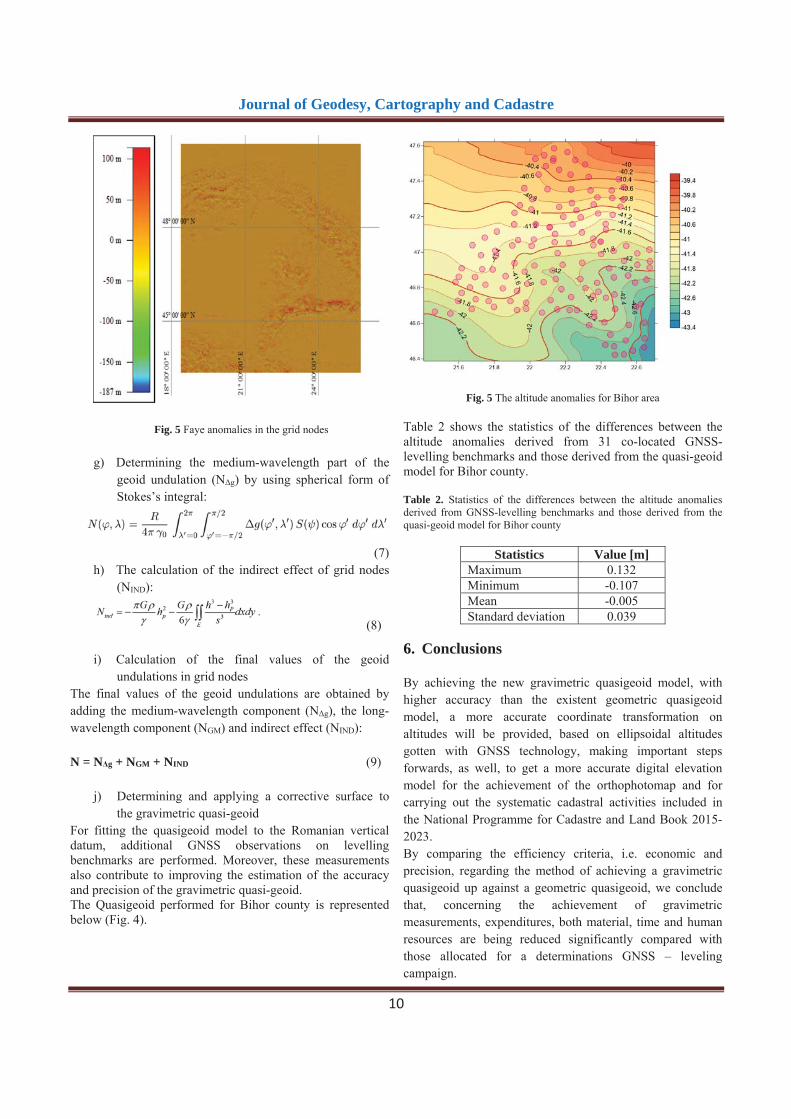
Fig. 5 Faye anomalies in the grid nodes g) Determining the medium-wavelength part of the

geoid undulation (N g) by using spherical form of Stokes’s integral:

(7)

h) The calculation of the indirect effect of grid nodes (NIND):

(8)

i) Calculation of the final values of the geoid undulations in grid nodes

The final values of the geoid undulations are obtained by adding the medium-wavelength component (N g), the long-wavelength component (NGM) and indirect effect (NIND): N = N g + NGM + NIND (9)

j) Determining and applying a corrective surface to

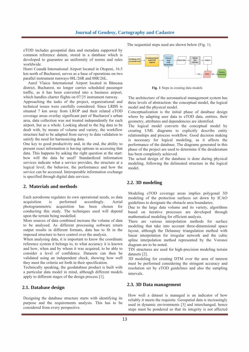
the gravimetric quasi-geoid For fitting the quasigeoid model to the Romanian vertical datum, additional GNSS observations on levelling benchmarks are performed. Moreover, these measurements also contribute to improving the estimation of the accuracy and precision of the gravimetric quasi-geoid. The Quasigeoid performed for Bihor county is represented below (Fig. 4).

Fig. 5 The altitude anomalies for Bihor area Table 2 shows the statistics of the differences between the altitude anomalies derived from 31 co-located GNSS-levelling benchmarks and those derived from the quasi-geoid model for Bihor county. Table 2. Statistics of the differences between the altitude anomalies derived from GNSS-levelling benchmarks and those derived from the quasi-geoid model for Bihor county

Statistics Value [m] Maximum 0.132 Minimum -0.107 Mean -0.005 Standard deviation 0.039

6. Conclusions

By achieving the new gravimetric quasigeoid model, with higher accuracy than the existent geometric quasigeoid model, a more accurate coordinate transformation on altitudes will be provided, based on ellipsoidal altitudes gotten with GNSS technology, making important steps forwards, as well, to get a more accurate digital elevation model for the achievement of the orthophotomap and for carrying out the systematic cadastral activities included in the National Programme for Cadastre and Land Book 2015-2023. By comparing the efficiency criteria, i.e. economic and precision, regarding the method of achieving a gravimetric quasigeoid up against a geometric quasigeoid, we conclude that, concerning the achievement of gravimetric measurements, expenditures, both material, time and human resources are being reduced significantly compared with those allocated for a determinations GNSS – leveling campaign.


11

The new quasigeoid model and its applications will have implications in most areas of investment and achievement of national projects including those relating to agricultural work, the water management, studies concerning hydro and hydropower accumulation, transport, air navigation, satellite remote sensing, achieving of GIS specialized sites, environmental issues and ecology, seismic and geodynamic phenomena, achieving hazard and risk maps etc. References

[1] Andersen, O. B., Forsberg, R. - Danish precision gravity

reference network. KMS, Ser. 4, Vol. 4, Denmark, 1996 [2] Avramiuc, N., SC WEBSOFT SOLUTIONS SRL -

Raport de activitate privind prestarea serviciilor de dezvoltare a pachetului software TransDatRO - Realizarea modelului de cvasigeoid gravimetric pentru zona municipiului Bucure ti, 2012

[3] Bernhard Hofmann-Wellenhof, Helmut Moritz - Physical Geodesy, Wien, 2005

[4] Cunderl´Ik, R., Tenzer, R., Abdalla, A., Mikula, K. - The quasigeoid modelling in New Zealand using the boundary element method, Contributions to Geophysics and Geodesy Vol. 40/4, (283–297), 2010

[5] Forsberg, R., Tscherning, C.C. - The use of Height Data in Gravity Field Approximation by Collocation. J.Geophys.Res., Vol. 86, No. B9, pp. 7843-7854, 1981

[6] Ghi u, D. - Geodezie i gravimetrie geodezic , Bucure ti, 1983

[7] Hwang, Cheinway, Cheng-Gi Wang, Li-Hua Lee - Adjustment of relative gravity measurements using weighted and datum-free constraints, Department of Civil Engineering, National Chiao Tung University,

Taiwan, Computers & Geosciences 28, 1005 - 1015, 2002

[8] Marinescu, M., Tomoioag , T. – Tem de cercetare tiin ific dezvoltat în cadrul Agen iei de Cercetare

pentru Tehnic i Tehnologii Militare, beneficiar Direc ia Topografic Militar – ”Geoid pentru teritoriul României, determinat pe baza modelului geopoten ial global EGM96 i a re elei gravimetrice militare”, Bucure ti, 1998

[9] Moldoveanu, C. - Geodezie, Bucure ti, 2002 [10] Oja, T. - New solution for the Estonian gravity

network GV-EST95, 7th International Conference Environmental Engineering (1409 - 1414), Vilnius: VGTU Press "Technika", 2008

[11] Sans`o, F., Sideris, M. G. - Geoid Determination. Theory and Methods., London, 2013

[12] Sorta, V. – Tez de doctorat - Contribu ii la determinarea cvasigeoidului pe teritoriul României, Bucure ti, 2013

[13] Spiroiu, I. – Tez de doctorat – Contribu ii la elaborarea metodelor de determinare cu o rezolu ie superioar a ondula iilor geoidului în re elele geodezice tridimensionale, Bucure ti, 2005

[14] Tomoiag , T. S. – Tez de doctorat – Contribu ii privind determinarea ondula iilor geoidului folosind modelele geopoten iale globale i date gravimetrice locale, Bucure ti, 2007

[15] Torge, W. - Geodesy, Berlin, New York, 2001 [1] Weikko A. Heiskanen, Helmut Moritz, Physical

Geodesy, Graz, 1993 [2] www.roadsbridges.com/bridges (Aug. 2017) [3] www.iptana.ro (Aug. 2017)


12

Smart Managing Aeronautical Data

Sabina Pl vicheanu1, Florin Nache2, Petre Iuliu Dragomir3

Received: April 2016 / Accepted: September 2016 / Published: December 2017 © Revista de Geodezie, Cartografie i Cadastru/ UGR Abstract This research study focuses on the individuality and complexity of aeronautical data, considering both acquisition and processing methods to be customized to this field. Aeronautical information is integrated into GIS environment that is designed for the needs of this industry, where standardization and interoperability are the key elements, data quality requirements are higher and accurate coordinates are essential for aeronautical safety. The goal is to design efficient database management systems, able to store, analyse, validate and manipulate spatial data, according to the applicable aeronautical regulations. Keywords Aeronautical data, GIS, Obstacle assessment, Interoperability

1. Introduction In order to improve the accuracy and safety of air traffic in a coordinated and structured manner, each ICAO signatory

country adheres to standardizing data exchange. While meeting the international standards, some countries (e.g. United Kingdom, United States of America, United Arab Emirates, etc.) have issued their own modified versions of ICAO specifications to fulfill local conditions. Two of the main international airports in Romania, Henri Coand International Airport (LROP) and Aurel Vlaicu International Airport (LRBS), which are managed by Bucharest Airports National Company, have recently implemented eTOD (electronic Terrain and Obstacle Data) complying to ICAO requirements, providing precise and reliable digital information to underpin vital operations for Civil Aviation Authorities, airport authorities and airlines.

1 PhD. Student, Eng. Sabina Pl vicheanu

Technical University of Civil Engineering of Bucharest, Faculty of Geodesy,Romania, E-mail: [email protected] 2 PhD. Student, Eng. Florin Nache

University of Bucharest, Faculty of Geology and Geophysics, Romania, E-mail: [email protected] 3 Prof. PhD. Eng. Petre Iuliu Dragomir

Technical University of Civil Engineering of Bucharest, Faculty of Geodesy,Romania, E-mail: [email protected]


13

eTOD includes geospatial data and metadata supported by common reference datum, stored in a database which is developed to guarantee an uniformity of norms and rules worldwide. Henri Coand International Airport located in Otopeni, 16.5 km north of Bucharest, serves as a base of operations on two parallel instrument runways 08L/26R and 08R/26L.

Aurel Vlaicu International Airport located in B neasa district, Bucharest, no longer carries scheduled passenger traffic, as it has been converted into a business airport, which handles charter flights on 07/25 instrument runway. Approaching the tasks of the project, organizational and technical issues were carefully considered. Since LRBS is situated 7 km away from LROP and their related eTOD coverage areas overlay significant part of Bucharest’s urban area, data collection was not treated independently for each airport, but as a whole. Looking ahead to the big data to be dealt with, by means of volume and variety, the workflow structure had to be adapted from survey to data validation to satisfy the need for harmonizing data. One key to good productivity and, in the end, the ability to present exact information is having options in accessing that data. This happens by asking the right question at the start: how will the data be used? Standardized information services indicate what a service provides, the structure at a logical level, the behavior, the performance and how the service can be accessed. Interoperable information exchange is specified through digital data services. 2. Materials and methods Each aerodrome regulates its own operational needs, so data acquisition is performed accordingly. Aerial photogrammetric acquisition has been chosen for conducting this study. The techniques used will depend upon the terrain being modelled. More sources of data combined increase the volume of data to be analysed. As different processing software return output results in different formats, data has to fit in the imposed structure to have control over the analysis. When analysing data, it is important to know the coordinate reference system it belongs to, to what accuracy it is known and how, when and by whom it was acquired, to be able to consider a level of confidence. Datasets can then be validated using an independent check, showing how well they meet the criteria set forth in their specification. Technically speaking, the geodatabase product is built with a particular data model in mind, although different models apply to different stages of the design process [1]. 2.1. Database design Designing the database structure starts with identifying its purpose and the requirements analysis. This has to be considered from every perspective.

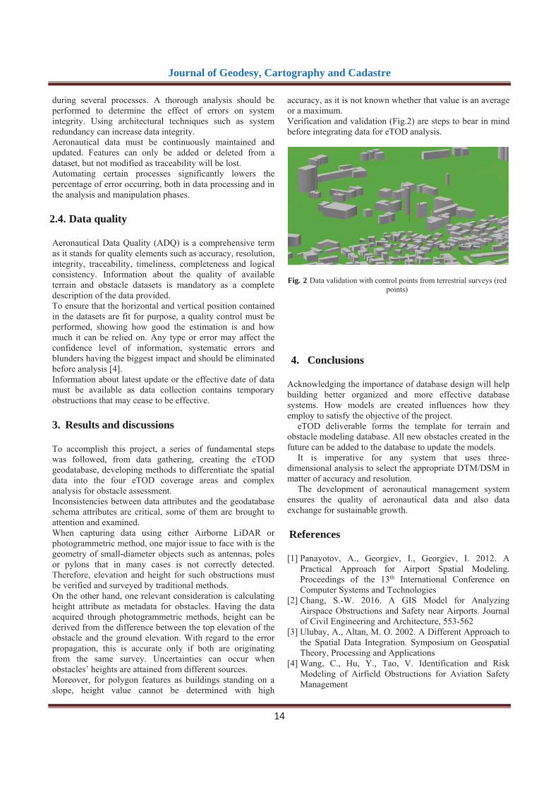
The sequential steps used are shown below (Fig. 1).

Fig. 1 Steps in creating data models

The architecture of the aeronautical management system has three levels of abstraction: the conceptual model, the logical model and the physical model. Conceptualization is the initial phase of database design where by adapting user data to eTOD data, entities, their geometry, attributes and dependencies are identified. The logical model converts the conceptual model by creating UML diagrams to explicitly describe entity relationships and process workflow. Good decision making is necessary for logical modeling, as it affects the performance of the database. The diagrams generated in this phase of the project are used to determine if the desideratum has been completely achieved. The actual design of the database is done during physical modeling, following the delineated structure in the logical model. 2.2. 3D modeling

Modeling eTOD coverage areas implies polygonal 3D modeling of the protection surfaces set down by ICAO guidelines to designate the obstacle area boundaries. Due to the large data volume and its variety, algorithms based on iterative processes are developed through mathematical modeling for efficient analysis. There are various interpolation methods for surface modeling that take into account three-dimensional space layout, although the Delaunay triangulation method with linear interpolation for irregular network and the cubic spline interpolation method represented by the Voronoi diagram are to be noted. TIN structures are used for high-precision modeling terrain datasets [2]. 3D modeling for creating DTM over the area of interest must be performed considering the stringent accuracy and resolution set by eTOD guidelines and also the sampling intervals.

2.3. 3D Data management

How well a dataset is managed is an indicator of how reliably it meets the requisite. Geospatial data is increasingly used in dynamic environments [3] and interchanged, hence steps must be pondered so that its integrity is not affected


14

during several processes. A thorough analysis should be performed to determine the effect of errors on system integrity. Using architectural techniques such as system redundancy can increase data integrity. Aeronautical data must be continuously maintained and updated. Features can only be added or deleted from a dataset, but not modified as traceability will be lost. Automating certain processes significantly lowers the percentage of error occurring, both in data processing and in the analysis and manipulation phases.

2.4. Data quality

Aeronautical Data Quality (ADQ) is a comprehensive term as it stands for quality elements such as accuracy, resolution, integrity, traceability, timeliness, completeness and logical consistency. Information about the quality of available terrain and obstacle datasets is mandatory as a complete description of the data provided. To ensure that the horizontal and vertical position contained in the datasets are fit for purpose, a quality control must be performed, showing how good the estimation is and how much it can be relied on. Any type or error may affect the confidence level of information, systematic errors and blunders having the biggest impact and should be eliminated before analysis [4]. Information about latest update or the effective date of data must be available as data collection contains temporary obstructions that may cease to be effective. 3. Results and discussions To accomplish this project, a series of fundamental steps was followed, from data gathering, creating the eTOD geodatabase, developing methods to differentiate the spatial data into the four eTOD coverage areas and complex analysis for obstacle assessment. Inconsistencies between data attributes and the geodatabase schema attributes are critical, some of them are brought to attention and examined. When capturing data using either Airborne LiDAR or photogrammetric method, one major issue to face with is the geometry of small-diameter objects such as antennas, poles or pylons that in many cases is not correctly detected. Therefore, elevation and height for such obstructions must be verified and surveyed by traditional methods. On the other hand, one relevant consideration is calculating height attribute as metadata for obstacles. Having the data acquired through photogrammetric methods, height can be derived from the difference between the top elevation of the obstacle and the ground elevation. With regard to the error propagation, this is accurate only if both are originating from the same survey. Uncertainties can occur when obstacles’ heights are attained from different sources. Moreover, for polygon features as buildings standing on a slope, height value cannot be determined with high

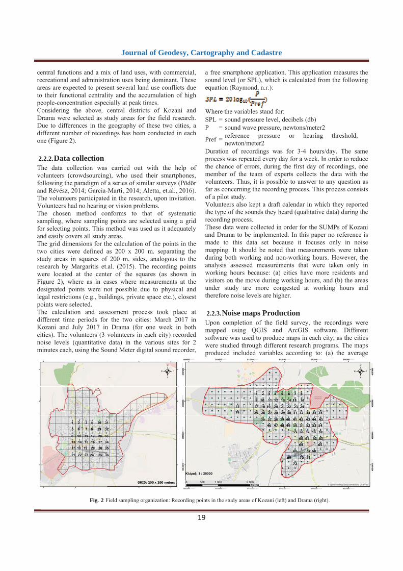
accuracy, as it is not known whether that value is an average or a maximum. Verification and validation (Fig.2) are steps to bear in mind before integrating data for eTOD analysis.

Fig. 2 Data validation with control points from terrestrial surveys (red

points)

4. Conclusions

Acknowledging the importance of database design will help building better organized and more effective database systems. How models are created influences how they employ to satisfy the objective of the project.

eTOD deliverable forms the template for terrain and obstacle modeling database. All new obstacles created in the future can be added to the database to update the models.

It is imperative for any system that uses three-dimensional analysis to select the appropriate DTM/DSM in matter of accuracy and resolution.

The development of aeronautical management system ensures the quality of aeronautical data and also data exchange for sustainable growth. References

[1] Panayotov, A., Georgiev, I., Georgiev, I. 2012. A

Practical Approach for Airport Spatial Modeling.Proceedings of the 13th International Conference on Computer Systems and Technologies

[2] Chang, S.-W. 2016. A GIS Model for Analyzing Airspace Obstructions and Safety near Airports. Journal of Civil Engineering and Architecture, 553-562

[3] Ulubay, A., Altan, M. O. 2002. A Different Approach to the Spatial Data Integration. Symposium on Geospatial Theory, Processing and Applications

[4] Wang, C., Hu, Y., Tao, V. Identification and Risk Modeling of Airfield Obstructions for Aviation Safety Management


16

The use of VGI in noise mapping Efthimios Bakogiannis1, Charalampos Kyriakidis2, Maria Siti3, Nikolaos Kougioumtzidis4 and Chryssy Potsiou5

Received: April 2016 / Accepted: September 2016 / Published: December 2017 © Revista de Geodezie, Cartografie i Cadastru/ UGR

Abstract The quality of the soundscape in urban spaces is significant for the total environment of a sustainable city. However, limited attention has been given to the acoustic environment of a city by planners. In Greece, research on this issue and its representation at the city scale has been conducted only in a limited number of large cities whereas in most of the cities and towns there is no available data. The aim of this paper is to present an overview of a research about the monitoring of the urban acoustic environment affordably and reliably, and investigating the potential of VGI for such applications for typical medium-sized cities. This research is conducted as part of the ongoing Sustainable Urban Mobility Plans project (SUMPs), aiming to improve the urban landscape, increase quality of life and transform cities into more compact urban cores. 1 Dr. E. Bakogiannis

Department of Geography and Regional Planning/School of Rural and Surveying Engineering/National Technical University of Athens 9, Iroon Polytechniou, Zografou Campus 15780, Athens Greece. E-mail: [email protected]

2 c. Ph.D. C. Kyriakidis Department of Geography and Regional Planning/School of Rural and Surveying Engineering/National Technical University of Athens 9, Iroon Polytechniou, Zografou Campus 15780, Athens Greece. E-mail: [email protected]

3.c. Ph.D. M. Siti Department of Geography and Regional Planning/School of Rural and Surveying Engineering/National Technical University of Athens 9, Iroon Polytechniou, Zografou Campus 15780, Athens Greece. E-mail: [email protected]

4.Und. Student N. Kougioumtzidis School of Rural and Surveying Engineering/National Technical University of Athens 9, Iroon Polytechniou, Zografou Campus 15780, Athens Greece. E-mail: [email protected]

5.Prof. Chryssy Potsiou Department of Topography/School of Rural and Surveying Engineering/National Technical University of Athens 9, Iroon Polytechniou, Zografou Campus 15780, Athens Greece.

E-mail: [email protected]

Once the urban design characteristics are listed by the experts, audio recordings are collected through crowdsourcing (using smart phones and apps) in several city spots, according to a grid-based sampling methodology. Then, a sound map is created using an Ordinary Kriging technique in GIS, while finally the collected noise data are imported in OpenStreetMap (OSM) by the volunteers. The methodology was tested in two Greek medium-sized city centers (Kozani, and Drama). The soundscape data were then assessed by taking into consideration the European and national legislation about the urban acoustic environment as well as the various characteristics of each case-study area. As expected, results show that residents are exposed to high sound levels during the day. However, sound levels in car-free zones are considerably lower except from specific streets where motorcycles enter illegally (for delivery or freight purposes). In overall, this research proved that there is a p[potential of using crowdsourcing technique to collect noise data and monitor the soundscape reliably and affordably. It is crucial for the municipalities to activate citizens in participating to urban renewal projects in main streets as well as in vulnerable city areas (i.e. neighborhoods, school zones) in order to raise awareness about noise maps and create a better acoustic environment. Through these case studies, this paper points out that crowdsourced noise mapping may be utilized as a reliable tool for participatory planning. The paper provides considerations about how the proposed methodology may be further tested and improved. Keywords Sustainable mobility, urban planning, acoustic environment, soundscape mapping, ordinary kriging method, Open Street Map, VGI, crowdsourcing.


17

1. Considering new technologies for the recording of the sonic environment of the cities Over 50 years have passed since Murray Schafer studied the influence of the sonic environment on people. However, the term “soundscape”, which was used to explain the relation presented above (Rodriguez-Manzo, et.al., 2015 · Schulte-Fortkamp and Jordan, 2016), is still up-to-date. Another up-to-date issue has to do with the transformations of the soundscape. In contrast with the natural and urban environment where the differentiations could be easily understandable through aerial photography techniques of remote sensing and mapping tools, the investigation of the changes that occur in the soundscape (Schaffer, 1993) is not easy due to the fact that, in many areas, mappings of the soundscape are not carried out although they constitute usefulness for the evaluation of buildings and urban areas (Schulte-Fortkamp and Jordan, 2016). The view of Maffei, et.al. (2012) and Margaritis, et.al.(2015) that the sonic environment did not consist of a significant parameter in the urban planning practice is well-founded even in Greece where the only official mapping of the soundscape has been carried out between 2012-2016 only in specific cities based on the 13586/724/2006 Joint Ministerial Decision (FEK B’ 384) that harmonizes the European Directive 2002/49/ C (Vogiatzis and Remy,2017), aimed at confronting high levels of noise in cities using common ways for all the country members (Stoter, et.al., 2008 · Licitra and Memoli, 2008). However, these mapping projects do not constitute a complete representation of the sonic environment but only of the environmental noise [Strategic Noise Maps (S.N.M) and Noise Action Plans(N.A.P.)] (Directive 2002/49/EC), which is only a parameter of the sonic environment according to Rodriguez-Manzo et.al.(2015). The reason for interest in noise has to do with the fact that noise pollution is an essential problem in urban areas (Schweizer, et.al., 2011 · Pödör and Révész, 2014 · Pödör, et.al., 2015 · Rodriguez-Manzo, et.al., 2015 · Poslon ec-Petri , et.al., 2016 · Pödör and Zentai, 2017). Indeed, Vasilev (2017) points out that increase of the levels of noise (0,5-1,0 dBA) in the cities is a reality. Regarding the measurement and monitoring of noise levels, different methodologies have been occasionally suggested. Such methodologies are noise recordings, population surveys and interviews, soundwalks and noise mapping (Rodriguez-Manzo, et.al., 2015 · Schulte-Fortkamp and Jordan, 2016). Even for individual procedures, different techniques have been proposed. In noise mapping, for instance, different methods and tools could be used (Bennett et al.,2010-Schulte-Fortkamp and Jordan,2016) for data collection and representation. Indeed, according to Schulte-Fortkamp and Jordan (2016), the natural conditions of a soundscape can be measured by using binaural recording devices or microphone arrays. Maps can be created by algorithms that produce maps based on estimations or by using measured data (Cho, et.al., 2007 ·

Stoter, et.al., 2008). In practice, due to high cost (Schweizer, et.al., 2011), local authorities choose to monitor soundscape by placing sensors in specific indicative points, that usually do not cover the total surface of a city. According to Aiello, et.al. (2016), this particular method is a result of the European Directive 2002/49/ C which requires European countries to monitor noise levels that were produced by specific sources (road traffic, railways, airports and industry). The same researchers (Aiello, et.al., 2016) point out that, due to many deficiencies observed, epidemiological models are occasionally used for estimating noise levels. These models are based on samples of small population or data derived from smartphones or social media, in order to decrease the cost of such researches. The researches of Podor and Revesz (2014), Podor et al. (2015) and Podor and Zentai (2017) converge to the same opinion and argue that is fundamental to use data derived from crowdsensoring and crowdsourcing for monitoring noise levels. That is why, according to the European Directive 2002/49/ C, noise maps must be renewed every 5 years something not easy taking into consideration the economic conditions of certain countries such as Hungary, to which these researches are referred, if the methods used are conventional. During recent years, the European Commission has financed projects that are based on crowdsourcing in which people have been used as “sensors” (Podor, et.al., 2015). In these projects, people carry their smartphones that are personal devices equipped with applications that provide data without cost (Schweizer, et.al., 2011). According to Schweizer, et.al., 2011 the smartphones constitute ideal platforms for environmental data measurements because, beyond sound levels that are recorded by the microphone which is incorporated in the device, they are also equipped with GPS providing spatial information, at the same time. The advantages of smartphones can be used in order for researchers to achieve goals like: (a) low-cost data collection process, (b) citizen’s participation for improving the quality of urban environment and (c) constant monitoring of the soundscape, when people use applications providing real time data. From the above, it can be concluded that the participation of people consists of a significant process on which this paper focuses. The reasons are: (a) volunteered participation is a necessary parameter in order to collect data with low-cost budget(Schulte-Fortkamp and Jordan, 2016), (b) volunteered participation has a great additional value as it constitutes a process that increases the geospatial maturity of the society to understand the design procedures and various planning matters (Athanasopoulos and Stratigea, 2015 · Bakogiannis, et.al., 2017) and (c) the participation of people is an example of direct democracy that seals the transparency and the social consensus through a structured dialogue procedure and interaction (Kyriakidis, 2012). Based on the above, in this paper a methodology is proposed for noise data collection by volunteers who used a specific application in their smartphones. In the next unit, the testing of the proposed method for Kozani and Drama, Greece, is presented, in detail.


18

Fig. 1 Block diagram of the proposed methodology

2. Methodology

2.1. Aim and Objectives Considering that noise mapping is required only for major cities of each EU member country, and considering the lack of financial resources of some EU states (e.g., Greece) to meet this requirement and to expand this practice to other cities (e.g., mid-sized cities), it is worthwhile questioning to what extent crowdsourcing technique could help to create noise maps for mid-sized cities. Thus, the aim of this paper is to develop a methodology for noise monitoring. This methodology should be easily applicable, reliable and cost-effective. These case studies presented here are for Greece where Sustainable Urban Mobility Plans (SUMP) are implemented. The above research question is well-founded given the fact that the soundscape is essential for the promotion of well-combined urban and transport planning (e.g., reduction of noise levels in areas where it is particularly intense). Moreover, it could be used as an indicator for the SUMP by comparing the previous to the subsequent noise levels. The main objectives of this study are to: Examine if the results of surveys carried out by mobile equipment are satisfactory. Promote the concept of open noise data as far as concerning the cities under study, by uploading them in the Open Street Map (OSM).

2.2. Proposed Methodology In the literature (Rodriguez-Manzo, et.al., 2015 · Schulte-Fortkamp and Jordan, 2016), there are presented many ways for recording and mapping the cities’ soundscape. Such examples are soundwalks, sound recordings and interviews with experts and locals. However, according to current research, participation of citizens consists of a usual process in smart cities’ projects (Poslon ec-Petri , et.al., 2016). This trend is related to the time-consuming process of traditional noise mapping as well as to the cost of its implementation. Indeed, the methodology which is normally used for producing strategic noise maps includes the existence of data-sets such as 3D digital ground models, city traffic models, train traffic models (in case a train station is located in the city under study) and the use of an ideal software for mapping the sound levels (Garai and Fattori, 2009). In many cities of Europe (e.g., most of the Greek cities) there are no available data of such type and their collection is costly. According to the Report “Best Practice in Strategic Noise Mapping” which was drawn up by the subgroup END noise mapping of the CEDR Project Group Road Noise 2 (2013), the cost of noise mapping is significant; an approximate estimation of the average total cost for noise mapping per km mapped is € 604. In this research which was conducted on Kozani and Drama, a new methodology was used in order for mapping the noise in these two cities. The new methodology is graphically presented in Figure 1. Although this methodology differs from the one that is usually preferred, however, it could be an easily applicable and cost-effective alternative for monitoring noise, mainly in small and mid-sized cities. It is also important that through importing data into OSM it is possible to create an interactive noise map. The next step in this research will be to put in place a dynamic map in which the data collected by the residents through their smartphones will be presented simultaneously on the map. In that way, noise will be constantly monitored. For the research in Kozani and Drama, the methodology was organized as presented below. 2.2.1.Study areas selection The cities chosen for this research are medium-sized cities of Greece. Kozani is located in the Region of West Macedonia, Greece; and its population (2011 census) is 41.066 residents. Drama is located in the Region of Eastern Macedonia, Greece and Thrace; and its population (2011 census) is 44.823 residents. They were selected for this paper due to their common characteristics (e.g. they have almost the same population; their central districts have been developed without plan over the centuries; important roads are crossing at their central districts; their central districts mainly display analogous land use dispersion and clustering; Neither S.N.M. nor N.A.P. has been conducted for Kozani and Drama as they are medium-sized cities and there is no obligation to implement them, according to Dir. 2002/49/EC). The study areas in these two cities involve a number of


19

central functions and a mix of land uses, with commercial, recreational and administration uses being dominant. These areas are expected to present several land use conflicts due to their functional centrality and the accumulation of high people-concentration especially at peak times. Considering the above, central districts of Kozani and Drama were selected as study areas for the field research. Due to differences in the geography of these two cities, a different number of recordings has been conducted in each one (Figure 2). 2.2.2.Data collection The data collection was carried out with the help of volunteers (crowdsourcing), who used their smartphones, following the paradigm of a series of similar surveys (Pödör and Révész, 2014; Garcia-Marti, 2014; Aletta, et.al., 2016). The volunteers participated in the research, upon invitation. Volunteers had no hearing or vision problems. The chosen method conforms to that of systematic sampling, where sampling points are selected using a grid for selecting points. This method was used as it adequately and easily covers all study areas. The grid dimensions for the calculation of the points in the two cities were defined as 200 x 200 m. separating the study areas in squares of 200 m. sides, analogous to the research by Margaritis et.al. (2015). The recording points were located at the center of the squares (as shown in Figure 2), where as in cases where measurements at the designated points were not possible due to physical and legal restrictions (e.g., buildings, private space etc.), closest points were selected. The calculation and assessment process took place at different time periods for the two cities: March 2017 in Kozani and July 2017 in Drama (for one week in both cities). The volunteers (3 volunteers in each city) recorded noise levels (quantitative data) in the various sites for 2 minutes each, using the Sound Meter digital sound recorder,

a free smartphone application. This application measures the sound level (or SPL), which is calculated from the following equation (Raymond, n.r.):

Where the variables stand for: SPL = sound pressure level, decibels (db) P = sound wave pressure, newtons/meter2

Pref = reference pressure or hearing threshold, newton/meter2

Duration of recordings was for 3-4 hours/day. The same process was repeated every day for a week. In order to reduce the chance of errors, during the first day of recordings, one member of the team of experts collects the data with the volunteers. Thus, it is possible to answer to any question as far as concerning the recording process. This process consists of a pilot study. Volunteers also kept a draft calendar in which they reported the type of the sounds they heard (qualitative data) during the recording process. These data were collected in order for the SUMPs of Kozani and Drama to be implemented. In this paper no reference is made to this data set because it focuses only in noise mapping. It should be noted that measurements were taken during both working and non-working hours. However, the analysis assessed measurements that were taken only in working hours because: (a) cities have more residents and visitors on the move during working hours, and (b) the areas under study are more congested at working hours and therefore noise levels are higher. 2.2.3.Noise maps Production Upon completion of the field survey, the recordings were mapped using QGIS and ArcGIS software. Different software was used to produce maps in each city, as the cities were studied through different research programs. The maps produced included variables according to: (a) the average

Fig. 2 Field sampling organization: Recording points in the study areas of Kozani (left) and Drama (right).


20

value of the recorded noise levels; (b) the minimum values; and (c) the peak values for the working hours. The mapping process is usually implemented by using various interpolation techniques (Margaritis, et.al., 2015). Li and Heap (2008) present 26 interpolation techniques that are quite similar and can be performed for mapping processes. Geymen and Bostanci (2012) support that Inverse Distance Wight Method (IDW), Ordinary Kriging Method (OK) and Redial Basis Functions Method (RBF) are three useful methods for noise mapping, as they have selected these techniques for representation of noise values. Margaritis et.al. (2015) underline that Kriging and IDW techniques are the most widely known in the field of noise mapping. However, through literature review (Geymen and Bostanci, 2012 · Aletta and Kang, 2015 · Margaritis, et.al., 2015), it was concluded that the Kriging technique is a powerful method that is most often used. That was the reason why Kriging methodology was selected for mapping in this study. The 2D raster surfaces were created based on the OK Method considering all the points of each study area. Adobe Photoshop CC14 was also used for improving the aesthetic of the maps. The analysis and mapping process presented above was conducted by the team of experts who were coordinating the data collection process. Finally, the maps were uploaded by volunteers in the Open Street Map platform in order to provide free access information for anyone interested. Due to the fact that volunteers were people with some technical skills, not much special training was necessary. However, in case volunteers need to be trained, a short training session could be organized in the initial stage of the field research. In this session instructions about the recording process should be given. 2.2.4. Limitations Research limitations are mainly related to the time frame of the research. The field research has been conducted at different times for each city because each research was a part of SUMPs the time frames and the deadlines of which were different. As for risk management, a moving vehicle could cause bodily injury and property damage to volunteers and researchers. Moreover, the volunteers had to conduct the research during spring and summer when the temperature is high and they had to be exposed in the sun for many hours a day. 3. Analysis and Results

Although the derived noise data were collected over a one week period in 2017 by volunteers who recorded noise at the street level, they gave us quite rational noise maps, as expected. On that basis, it could be supported that they are reliable enough to draw the conclusions presented below.

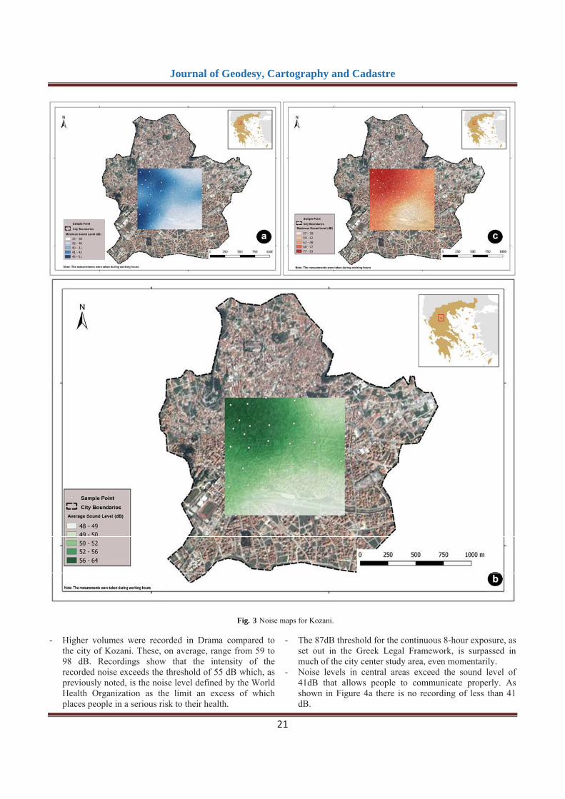
Using QGIS and ArcGIS, collected data were presented as a point feature layer. In order to realize where there is a spatial relationship among the values (minimum, maximum and mid values) represented by each point feature, the OK method was used. Figures 3 and 4 depict noise maps for each city studied (Kozani and Drama). The noise maps that were created by taking into account the mid values are the most important because they capture a more in-depth analysis by excluding extreme (min and max) values. The results for Kozani could be concluded in these points:

- High intensity noise was noticed in Kozani averaging from 39 to 64 dB. As seen in Figure 3b, sounds recorded in a large part of the study area are higher than 55 Db; the noise level defined by the World Health Organization as the limit at which people are at serious health risk.

- Higher intensity sounds were recorded at the northwest region of the study area, due to the following facts: (a) the existence of crucial streets (i.e. Dimokratias Str., Fon Kozani Str., Paulou Mela Str., M. Alexandrou Str.), (b) the concentration of a large number of commercial/ recreation stores and (c) administrative uses and points of high interest.

- Values higher than 84dB (Figure 3c) -sometimes ephemeral- were recorded in a large part of the city. This is a worrying fact, considering that the 87 dB threshold is the limit set by the Greek law (Presidential Decree 149/2006) for a maximum fixed exposure value for a worker in an 8-hour work day.

- Noise levels are relatively high, even in the case of the minimum values (30dB) recorded (Figure 3a), given the fact that levels higher than 23 dB can cause problems in the understanding of speech and thus the communication of people (Anon, n.r.). The intensity of the recorded sounds is higher in the northwest side of the study area, where the concentration of commercial/ recreational land uses is higher, and therefore the higher number of daily discussions is held, especially during working days and hours.

- The north-western part of the study area shows small fluctuations, as shown in Figures 3a-3c. Recorded sounds are mostly high during working hours (Figures 3a-3c). Minor fluctuations in sound intensity are also recorded in areas located in the east of the study area. St. George’s area, the University of West Macedonia campus area and spaces around OSE (inactive train station) are the quietest areas throughout the study area.

- Noise levels are the significant result of the urban environment. In the case of Kozani this is quite evident while observing the noise maps for the semi- pedestrianized city center where the smallest range of peak sound levels is observed, as opposed to the areas near major streets where larger peak sound levels are observed.

Similarly, the results for Drama can be concluded by the following key points:


21

- Higher volumes were recorded in Drama compared to the city of Kozani. These, on average, range from 59 to 98 dB. Recordings show that the intensity of the recorded noise exceeds the threshold of 55 dB which, as previously noted, is the noise level defined by the World Health Organization as the limit an excess of which places people in a serious risk to their health.

- The 87dB threshold for the continuous 8-hour exposure, as set out in the Greek Legal Framework, is surpassed in much of the city center study area, even momentarily.

- Noise levels in central areas exceed the sound level of 41dB that allows people to communicate properly. As shown in Figure 4a there is no recording of less than 41 dB.

Fig. 3 Noise maps for Kozani.


22

- Highest noise levels were recorded in central areas close to main streets that attract large numbers of motorized vehicles.

- The area around the OSE (inactive train station) appears to have low noise levels, although adverse results were expected. The local maximum levels are lower than those recorded at the center, while the overall highest in the area are relatively low. Overall there are small fluctuations observed in the area.

- As previously noted, the urban environment is significantly associated with noise levels. This is quite obvious in the case of Agia Varvara park, which seems

to function as a sound fence for its surroundings. The recorded average high and low sound levels in the vicinity of the park are significantly lower than those recorded throughout the city.

Summarizing the above, both cities encounter issues in terms of noise pollution. Pollution is higher in the city of Drama although there are larger green areas and measurements were taken in the summer period. The greater extent of urban morphology in Kozani, along with the latest pedestrianization projects in the city center, appear to be the two key elements contributing to the maintenance of lower noise levels.

Fig. 4 oise maps for Drama.


23

Fig. 4 Noise recordings in Kozani presented in OSM.

Fig. 5 Noise recordings in Drama presented in OSM As mentioned before, noise information for these two cities is now available through OSM. Figures 5 and 6 present a part of each city map in OSM, where the noise recordings are presented. Data were digitized by the volunteers who were not trained due to the fact that they were already familiar with the OSM. Instructions about the recording process have been given and a pilot study was also implemented. It should be mentioned that in case volunteers need to be trained, a short training session could be organized, as Figure 1 presents. 4. Conclusions Noise mapping is a strategy established for monitoring noise levels and protecting human health. Indeed, the European Directive 2002/49/EC proposed plans and maps which had to be implemented for specific cities and transport infrastructures. Through this Directive, a detailed methodology is proposed in which specific indicators should be used. Although the results of this method are accurate, however, this is a time-consuming and costly method. Thus, it is not possible to be applied in medium and small cities for which the compilation of noise studies is not compulsory by the law. In these cases, citizen participation may help in the collection and publishing of the data.

The aim of this paper is to develop a new methodology for noise mapping. This methodology should be easily applicable and cost-effective. Its rationale is based on community engagement and volunteering. The following steps outline a simple and effective strategy for mapping the noise levels in a city: Organizing the field systematic sampling. Preparing the volunteers who are responsible for collecting the data and digitizing them in the OSM. Pilot study. Collecting the data. Creating the maps while simultaneously the volunteers are uploading the data in the OSM. Publishing the maps. In cases of Kozani and Drama, the above methodology was applied. Three volunteers in each city participated in this project. They collected noise data for one week in each city by using their smartphones. More specifically, they have used one free app, named Sound Meter. These data are differentiated from the data that should be collected according to the Directive 2002/49/EC because: (a) they were collected at the street level, while the Directive imposed that the recording should take place in the height of 4 meters and (b) recordings lasted for approximately 3-4 hours/day while the Directive imposed that the recording should take place 24 hours/day. The first issue is a matter that should be further examined in order to adjust the proposed limits of noise exposure taking into account the height in which the recording are conducted. The second issue can be faced by attracting volunteers in large numbers. The more people participate, the more recordings will be implemented. However, taking into account the fact that there are no available data for many Greek cities (and elsewhere), through this methodology satisfactory information are provided that can be helpful for researchers in order to understand the soundscape of each city. This has become obvious through the case studies (Kozani and Drama) presented above. Through this methodology, in these cities, transport engineers, planners, decision makers and citizens can understand how important is to use sustainable means of urban transport and to minimize road surfaces within city centers. Indeed, through noise mapping in Kozani and Drama it was found that the street pattern (morphology, geometric characteristics, land use, etc) is related to its soundscape. More specifically, it was found that in semi-pedestrianized areas, the noise levels were lower while the opposite was observed in areas where roads with a high traffic load are located. It should be noticed that the recorded data are now presented on the OSM and are available (immediately and free of charge) for anyone for whom it is important. OSM functions as an interactive map from which citizens can easily find or transform the existing information which is presented in data point format. However, until now it has not been possible for citizens to look at the noise map produced by the team of experts. This is a problem which needs to be resolved in the next phase of this research. Also, an important step would be to put in place a dynamic map. A dynamic map may be


24

compiled with data which will be collected by the residents who will provide it by using specific apps through their smartphones by which noise will be constantly monitored. This specific research may play a catalytic role in informing and raising public awareness which is crucial for the compilation of the SUMP of these cities. In the future, it would be crucial to test this methodology in order to realize if it is applicable and provides accurate data. To sum up, the methodology proposed above has the potential to provide representative data in a cost-effective manner. Moreover, its use is based on community engagement and helps to inform people about the quality of life in their cities and the projects that may take place in the near future. Furthermore, these data are available to everyone through OSM. Finally, there is room for improvement in order for this methodology to be better applicable and readable while it can constantly provide noise information helping in noise monitoring at low cost. Thus, this methodology may be an important tool for planners and researchers as their aim is to contribute to the quality of city life. References [1] Aiello, L.M., Schifanella, R., Quercia, D. and Aletta, F.,

Chatty maps: constructed sound maps of urban areas from social media data, Royal Society Open Science, ISSN: 2054-5703, 3(3). pp. n.r., 2016, DOI: 10.1098/rsos.150690

[2] Aletta, F. and Kang, J., Soundscape approach integrating noise mapping techniques: a case study in Brighton, UK, Noise Mapping, ISSN: 2081-879X, 2(1), pp. 1-12, 2015, DOI: https://doi.org/10.1515/noise-2015-0001

[3] Aletta, F., Masullo, M., Maffei, L. and Kang, J., The effect of vision on the perception of the noise produced by a chiller in a common living environment, Noise Control Engineering Journal, ISSN: 2168-8710, 64(3), pp. 363-378, 2016, DOI: https://doi.org/10.3397/1/3763786

[4] Alferez, J.R., Vanhooreweder, B., Segues, F., Karkkainen, A., Giannopoulou, E. and Belluci, P., Report “Best Practice in Strategic Noise Mapping” [Online] Available at: http://goo.gl/GVwftf [Retrieved on August 2017]

[5] Anon, Chapter 7, n.r. [Online] Available at: https://eclass.gunet.gr/modules/.../file.../

%207%20-%20 .pdf [Retrieved on March 2017]

[6] Athanasopoulos, K. and Stratigea, A., Public participation in decision making process and the new legal framework for spatial and environmental planning [, 4th National Conference of Planning and Regional Development, Volos, 24-27 September 2015

[7] Bakogiannis, E., Kyriakidis, C., Siti, M. and Eleftheriou, V., Four stories for sustainable mobility in Greece, Transportation Research Procedia, ISSN: 2352-

1465,24, pp. 345-353, DOI: 10.1016/j.trpro.2017.05.101 [8] Bennett, G., King, E. A., Curn, J., Cahill, V., Bustamante,

F. and Rice, H. J., Environmental noise mapping using measurements in transit, Proceedings of ISMA, 2010

[9] Cho, D. S., Kim, J. H. and Manvell, D., Noise mapping using measured noise and GPS data, Applied acoustics, ISSN: 0003-682X, 68(9), pp. 1054-1061, 2007, DOI: https://doi.org/10.1016/j.apacoust.2006. 04.015

[10] Directive 2002/49/EC of the European Parliament and of the council of 25 June 2002 relating to the assessment and management of environmental noise. Official Journal of the European Communities, L 189/12 18.07.2002Garai, M. and Fattori, D., Strategic noise mapping of the agglomeration of Bologna, Italy, WIT Transactions on the Built Environment, 107. pp. 519-528, 2009, DOI: 10.2495/UT090461

[11] Garcia-Martí, I., Torres-Sospedra, J. and Rodríguez-Pupo, L. E., A comparative study on VGI and professional noise data, Connecting a digital Europe through location and place, Proceedings of the AGILE 2014 International Conference on Geographic Information Science, Castellon, 3-6 June 2014, ISBN: 9789081696043

[12] Geymen, A. and Bostanci, B., Production of geographic information system aided noise maps, FIG Working Week 2012: Knowing to manage the territory, protect the environment, evaluate the cultural heritage, Rome, 6-10 May 2012

[13] Kyriakidis, C., Citizen and city: Issues related in public participation in the process of spatial planning , 3rd Pan-Hellenic Conference of Planning and Regional Development , Volos, September 2012

[14] Li, J. and Heap, D., A Review of Spatial Interpolation Methods for Environmental Scientists, Cambera, Australia: Geoscience Australia, ISBN 978 1 921498 28 2 (webcopy)

[15] Licitra, G. and Memoli, G., Limits and advantages of good practice guide to noise mapping, Journal of the acoustical society of America, ISSN: 0001-4966, 123(5), pp. 1401-1406, 2008

[16] Maffei, L., Di Gabriele, M. and Aletta, F., Soundscape variation in a historical city centre due to new traffic regulation, Acoustics 2012, Hong Kong, 13-18 May 2012, DOI: 10.1121/1.4708901

[17] Margaritis, E. and Kang, J., Effects of open green spaces and urban form on traffic noise distribution, Forum Acusticum, Krakow, 7-12 September 2014,

[18] Margaritis, E., Aletta, F., Axelsson, O., Kang, J., Bootledooren, D. and Singh, R., Soundscape mapping in the urban context: A case study in Sheffield, 29th Annual AESOP 2015 Congress, Prague, July 13-16, 2015, DOI: 10.13140/RG.2.1.5026.1607

[19] Pödör, A. and Révész, A., Noise map: Professional versus crowdsourced data, Proceedings of the AGILE 2014 International Conference on Geographic Information Science, Castellon, 3-6 June 2014, ISBN: 9789081696043

[20] Pödör, A., Révész, A., Oscal, A. and Ladomerszki, Z.,


25

Testing some Aspects of Usability of Crowdsourced Smartphone Generated Noise Maps, GI Forum 2015-Journal for Geographic Information Science, ISBN: 978-3-87907-558-4/ISSN:2308-1708, 1, pp. 354-358, 2015, DOI: 10.1553/giscience2015s354

[21] Pödör, A. and Zentai, L., Educational aspects of crowdsourced noise mapping, In: Peterson, M. (ed.), Advances in Cartography and GIS Science: Selections from International Cartographic Conference 2017, ISBN: 978-3-319-57336-6 (eBook), Omaha, NE: Springer International Publishing, pp. 35-46, DOI: 10.1007/978-3-319-57336-6_3

[22] Poslon ec-Petri , V., Šlabek, L. and Frangeš, S., With the Crowdsourced Spatial Data Collection to Dynamic Noise Map of the City of Zagreb, International Symposium on Engineering Geodesy SIG 2016, Varaždin, Croatia, May 20–22, 2016

[23] Poslon ec-Petri , V., Vukovi b , V., Frangeša , S. and Ba i , Ž., Voluntary noise mapping for smart cities, ISPRS Annals of the Photogrammetry, Remote Sensing and Spatial Information Sciences, III-4/W1, ISSN: 2194-9050 (Internet and USB), pp. 131-137, 2016, DOI: 0.5194/isprs-annals-IV-4-W1-131-2016

[24] Raymond, J., Sound Wave Equations Calculator-Science Physics Formulas, n.r. [Online] Available at: http://www.ajdesigner.com/phpsound/sound_wave_equation_spl_sound_pressure_level.php [Retrieved on August 2017]

[25] Rodriguez-Manzo, F., Garay-Vargas, E., Garcia-Martinez, S., Lancon-Rivera, L. and Ponce-Patron, D., Moving towards the visualization of the urban sonic space through soundscape mapping, The 22nd International Congress on Sound and Vibration (ICSV22). ISBN: 9781510809031, Florence, Italy, July 12-16, 2015

[26] Schulte-Fortkamp, B. and Jordan, P., When soundscape meets architecture, Noise Mapping Open, ISSN: 2084-879X (electronic version), 3, pp. 216-231, 2016 DOI: https://doi.org/10.1515/noise-2016-0015

[27] Schafer, M., The soundscape: Our sonic environment and the tuning of the world, ISBN: 0892814551, 9780892814558, Simon and Schuster, 1993

[28] Schweizer, I., Bärtl, R., Schulz, A., Probst, F., & Mühläuser, M., NoiseMap-real-time participatory noise maps, Second International Workshop on Sensing Applications on Mobile Phones, 2011

[29] Stoter, J., De Kluijver, H. and Kurakula, V., 3D noise mapping in urban areas, International Journal of Geographical Information Science, ISSN: 13658824, 13658816, 22(8), pp. 907-924, 2008, DOI: http://dx.doi.org/10.1080/13658810701739039

[30] Vasilev, A., New methods and approaches to acoustic monitoring and noise mapping of urban territories and experience of it approbation in conditions of Samara region of Russia, Procedia Engineering, ISSN: 1877-7058, 176, pp. 669-674, 2017, DOI: https://doi.org/10.1016/j.proeng.2017.02.311

[31] Vogiatzis, K. and Remy, N., Soundscape design guidelines through noise mapping methodologies: An application to medium urban agglomerations, Noise Mapping, ISSN: 2081-879X, 4(1), pp. 1-19, 2017, DOI: https://doi.org/10.1515/noise-2017-0001


26

Monitoring the vertical and horizontal displacements of the Poiana M rului dam St nescu Roxana Augustina1, Nache Florin2, P unescu Cornel3

Received: April 2016 / Accepted: September 2016 / Published: December 2017 © Revista de Geodezie, Cartografie i Cadastru/ UGR Abstract This study presents the main steps that are needed in order to realise the monitoring of hydrotechnical constructions. The subject of this study is the Poiana Marului dam, situated on the BistraMarului River. The geometric levelling and also the microtriangulation and microtrilateration topographical measurements on the dam were made in two stages, at a six months interval. All these measurements represent the only external verification that emphasize, with a high accuracy level, the vertical and horizontal displacements that occur in the structure of the dam. Keywords: Dam, Geometric Levelling, Altitude, Displacements 1. Introduction The monitoring of the constructions' behavior over time occurred due to the need to obtain information about the real state of a structure, to observe its evolution and to detect the occurrence of new degradations. The monitoring of the hydrotechnical constructions' behavior takes place throughout the life of the hydrotechnical construction and has as a main role the maintenance of their safety and functionality in order to avoid the potential danger that these constructions represent for the settlements downstream (human but also significant material losses) .

1St nescu Roxana Augustina, Geodetic Engineer Cornel & Cornel Topoexim // E-mail: [email protected] 1Nache Florin, PhD Student University of Bucharest // E-mail: [email protected] 1 P unescu Cornel, PhD Engineer, University Professor University of Bucharest // E-mail: [email protected]

Due to the succession of rainy years and also to the sudden warming of spring in the Banat Mountains, exceptional amounts of rainfall overlapped the melting season, resulting in floods with catastrophic effects on most of the rivers in Cara -Severin County. In order to reduce the damaging effects of the water, there were carried out works of regularization and embankment of the riverbeds. Thus, a complex fitting out program was developed to ensure the protection of the localities and economic objectives along the main watercourses in the county. [1] Located on the BistraM rului River, a tributary of the Bistra River, the Poiana M rului Dam (Fig.1) is part of the Bistra-Poiana M rului-Ruieni-Poiana Rusc hydropower plant, being put into operation for the first time in 1992. [2]

Fig. 1The location of the Poiana Marului dam

This fitting out includes the Poiana M rului and Poiana Rusc dams, and the Ruieni and Râul Alb hydroelectric plants, as well as the secondary adduction Bistra - Lac Poiana M rului (16.902m), which ensures the accumulation of water flows (1.66 m³/s) from adjacent basins (the 5 secondary water captures: Bistra, Lupului, Bucova, Marga and Nierme ). Thus, a surface accumulation of 125 ha was obtained at the normal retention level (620 mdM) with a total volume of 96.2 mil m³. [2] The dam of Poiana M rului is a dam built from rockfills with clay core. The elevation of the dam crowning is of 625 m, with a maximum height of 125 m, a base width of 448 m, its total length being 408 m. The narrow area of the quays


27

bounded by the downstream river elbow and the change of orientation of the right slope and, upstream, the widening of the valley imposed the location of the dam. [2] The Poiana M rului dam is located about 25 km away from the town O elulRo u and captures the waters of a 204 km² basin. The access to this objective is achieved through the county road DJ 683 Z voi - M ru - Poiana M rului, which connects the town of O elulRo u with the tourist resort Poiana M rului. [2] Periodic monitoring of the constructions is carried out continuously assessing the safety status of the hydrotechnical objective by conducting geometric mean levelling measurements for observing possible vertical displacements, as well as microtriangulation measurements to determine the horizontal displacements undergone. These methods allow detection of safety deficiencies and the intervention by structural and/or non-structural measures to prevent the development of atypical phenomena or behaviors. 2. Methodology 2.1. Performing the measurements necessary to determine vertical and plane displacements 2.1.1. Performing geometric mean levelling measurements The altimetric monitoring network for the constructions of the hydroelectric power plant Poiana Marului is made up of 8 fundamental bench marks: RNSTC1 and RNSTC2, located near the dam keeper`s house, RN605S and RN605D, on berm 605, RN585S, on berm 585, RN565D, on berm 565, RN545S and RN545D located on berm 545m and 48 monitoring bench marks, located on the downstream berms of the dam, on the crowning respectively (Fig. 2). Out of these, the fundamental bench marks RN585S and RN545D were not identified in the field because either they were destroyed, covered or inaccessible.

Fig. 2The crest and the 4 berms

For the levelling measurements, the Leica digital level 250M, 3 m fibre glass barcode staff were used, the precision being ± 0.7 mm/double km of levelling. To detect the vertical displacements, the geometric levelling with two horizons, was chosen as a method of measurement. The measurements were made by the same operator, with the same instrument and staff set. The readings on the staffs were performed so that the settling error of the instrument and of the staffs was eliminated (Back-Front-Front-Back method). The degradation error of the staffs' soles was also eliminated, beginning and ending the traverse with the same staff, and the spans had lengths of less than 25 m. No measurements were made when the mirage phenomenon occurred, when the lighting conditions were low or the humidity level was high 2.1.2. Realizing themictrotriangulation measurements The microtriangulation network consists of six pilasters B1, B6N, B7 and B8 left bank; two pilasters B4, B5 - right bank and 39 monitoring marks (Fig. 3). The type of pilasters is cylindrical, with Wild type force centering devices, not protected by thermal insulation. The access to the pilasters and berm marks was properly done, except for pillars B1, B6N and B7. At these pilasters the access was difficult because of the absence of the road, the access to them could only be made through the swamp or on steep slopes. The monitoringplanimetric network is distributed as follows:

12 marks numbered from R37 to R47 are located on the crowning, on the downstream side.

10 marks numbered from R27 to R36 on the berm at elevation 605,

6 marks denoted from R10 to R15 on the berm at elevation 585,

6 marks denoted from R16 to R21 on the berm at elevation 565,

5 marks denoted from R22 to R26 on the berm at elevation 545.

Fig. 3Pilasters and monitoring markers


28

For the microtriangulation stage, the measurements were performed with the TS 06 Plus total station produced by Leica, which provides a 1" precision in determinig the directions. The measurement method used for microtriangulation was the method of the series, from each stationed pilaster being made 4 series of measurements. As in the case of the geometric levelling, the measurements were performed by the same operator, with the same device and under optimum temperature, lighting and humidity conditions. 2.2. Processing of measurements to determine vertical and planimetric displacements In order to determine the fundamental fixed bench marks, the network they are forming was compensated as being free, and at the end the global congruence test was applied, together with the statistical Fischer test, to determine the existence of the displacements, and the Student test for locating the eventual displacements. In order to determine the elevations of the bench marks set on the crowning, a traverse levelling closed on the starting point was made, considering the bench mark RN 605D, on the berm 605, as being fixed. To determine the elevations of the monitoringbench marks located on the berms 605 and 585, the fundamental bench marks RN605S and RN605D were considered as being fixed, for the berm 565 - the bench mark RN565D, and for berm 545 – the bench mark 545S. The compensation of the levelling network was achieved by the conditional measurements method, proceeding identically for both periods (October 2016 and April 2017). The compensation of the microtriangulation network was done in block, using the leasts square method. Prior to the compensation, stable pilasters were identified by applying the statistical tests used in the geometric levelling. The constraint of the microtriangulation network was made on pilasters B4, B6N, B7 and B8.

3. Results Table 1 shows the values of the vertical displacements in relation to period 0, but also between the two measurement periods.

Tabel 1Vertical displacements

POIANA MARULUI DAM Oct. 2016

- Apr. 2017 [mm]

Differences between the current and main stage[mm] NAME

OF CONST

R.

NO. OF MARK

ER

ELEVATION 0

[m]

Oct. 2016

Apr. 2017 Obs.

BE

RM

545

RN545D 546.4640 - - not

found

RN545S 539.1974 0 0 stable RN1-22 545.7570 -108.0 -107.5 0.4 RN1-23 545.5310 -181.5 -181.1 0.4 RN1-24 545.4890 -110.0 -109.5 0.5

POIANA MARULUI DAM Oct. 2016

- Apr. 2017 [mm]

Differences between the current and main stage[mm] NAME

OF CONST

R.

NO. OF MARK

ER

ELEVATION 0

[m]

Oct. 2016

Apr. 2017 Obs.

RN1-25 545.6560 -131.2 -130.1 1.2 RN1-26 545.7970 -40.4 -38.6 1.8

FH1 545.8150 - - not found

FH3 546.7980 - - not found

BE

RM

565

RN565D 565.9916 0 0 fix

RN2-16 565.1620 -48.6 -49.8 -1.2 RN2-17 565.2430 -163.2 -165.7 -2.4 RN2-18 565.0240 -161.2 -165.0 -3.7 RN2-19 565.2550 -176.2 -180.1 -3.9 RN2-20 565.1280 -117.6 -120.8 -3.2 RN2-21 565.5320 -66.5 -68.2 -1.7

BE

RM

585

RN585S 590.8540 - - not

found

RN3-10 585.8720 -200.6 -207.4 -6.7 RN3-11 585.4550 -197.8 -202.9 -5.2 RN3-12 585.4700 -196.8 -201.3 -4.5 RN3-13 585.4390 -276.9 -281.1 -4.2 RN3-14 585.6090 -233.3 -238.3 -4.9 RN3-15 585.8000 -206.8 -213.8 -7.0

FH11 587.6700 - - not

found

FH2 586.6440 - - not

found

BE

RM

605

RN605S 604.7008 0 0 fix RN4-36 605.8790 -128.8 -130.5 -1.7 RN4-35 605.1640 -242.4 -246.1 -3.7 RN4-34 604.9140 -299.0 -303.9 -4.9 RN4-33 604.8970 -309.0 -314.4 -5.4 RN4-32 604.9880 -366.7 -372.3 -5.6 RN4-31 604.7460 -366.7 -372.0 -5.3 RN4-30 604.8000 -348.6 -353.8 -5.1 RN4-29 604.9720 -344.1 -348.0 -3.9 RN4-28 604.9230 -240.0 -242.0 -1.9 RN4-27 605.2390 -86.4 -84.8 1.6 RN605

D 607.4350 0 0 fix

FH12 605.2730 - - not

found

FH13 605.4460 - - not

found

DA

M C

RO

WN

ING

RN5-37 625.2540 -169.2 -177.0 -7.7 RN5-38 625.7090 -260.5 -267.2 -6.6 RN5-39 625.9890 -276.7 -284.5 -7.8 RN5-40 625.9090 -279.6 -286.6 -7.0 RN5-41 625.9790 -258.5 -265.5 -7.0 RN5-42 626.0190 -372.3 -382.2 -10.0 RN5-43 625.9810 -355.7 -364.2 -8.5 RN5-44 625.7910 -338.6 -347.8 -9.2 RN5-45 625.6640 -284.7 -292.9 -8.2 RN5-46 625.4500 -214.9 -221.9 -7.0 RN5-47 625.2720 -105.2 -112.3 -7.1 RN5-48 625.1750 -17.1 -23.7 -6.7


29

The vertical displacements of the last 5 periods are represented graphically (Fig. 4).

Fig. 4Vertical displacements in realtion to period 0 of the last 5 measurement periods

Table 2 shows the horizontal displacements in relation to the period 0 of the 2 periods but also the planimetric displacements between the two periods(November 2016 and April 2017).

Axis X is oriented to the right bank and the Y axis upstream, so the positive displacements will be upstream and towards the right bank.

Tabel 2Horizontal displacements

FOLLOW UP OF THE BEHAVIOR OF THE HYDROTECHNICAL CONSTRUCTIONS

PLANIMETRIC DISPLACEMENTS Poiana M rului

Typ

e

Nam

e

PeriodNoiembrie 2016

PeriodAprilie 2017

Displacements 2016 -2017 Obs.

L-R-DR

AV-AM L-R AV-

AM L-R AV-AM

2016 2016 2017 2017 2016

- 2017

2016 -

2017

x [mm]

y [mm]

x [mm

]

y [mm]

x [mm

]

y [mm

]

PIL

AST

ER

S

B1 14.2 0.7 14.7 -4.9 0.5 -5.6B2 0 0 0.9 -14.7 0.9 -14.7B4 0 0 0 0 0 0 fixed B5 6.1 -3.4 -6 -3.3 -12.1 0.1 B6 -10 4 -9.3 0.3 0.7 -3.7

B6N 0 0 0 0 0 0 fixed B7 0 0 0 0 0 0 fixed B8 0 0 0 0 0 0 fixed

MO

NIT

OR

ING

MA

RK

ERS

R10 41.8 -49 40.2 -65.9 -1.6 -16.9R11 40 -62.1 39.5 -78.5 -0.5 -16.4R12 44.8 -48.5 38.2 -61.8 -6.6 -13.3R13 21.2 -36.9 15 -48.4 -6.2 -11.5R14 -66.5 -73.3 -74.1 -84 -7.6 -10.7R15 -56.4 -57.5 -58.2 -64.1 -1.8 -6.6R16 -59.6 -69.2 -68.2 -72.5 -8.6 -3.3R17 -68.7 -85.9 -72.2 -87 -3.5 -1.1R18 -45.8 -60.4 -52.4 -72.8 -6.6 -12.4R19 23.8 -60.2 18.2 -68.2 -5.6 -8R20 77.7 -62.7 78.6 -75.4 0.9 -12.7R21 55.5 -62.6 55.2 -67.5 -0.3 -4.9R22 -17.5 -77.2 -18 -77.5 -0.5 -0.3R23 63 -67.4 52.4 -74.3 -10.6 -6.9R24 -56.3 -53.5 -60.9 -65.4 -4.6 -11.9R25 -17.4 -79.7 -28 -93 -10.6 -13.3R26 -51.6 -80.3 -51.3 -85.4 0.3 -5.1

R27 not found

R28 -78.6 -68.8 -86.7 -74.5 -8.1 -5.7

R29 not found

R30 -30.4 -81.9 -37.6 -100.8 -7.2 -18.9R31 -39.2 -60 -38.5 -76.6 0.7 -16.6R32 56.2 -65.5 51.2 -84.2 -5 -18.7R33 68.9 -49.8 71.9 -68.9 3 -19.1R34 28.9 -50.5 34.1 -68.5 5.2 -18R35 72.9 -44 73.2 -59.6 0.3 -15.6R36 75.3 -61.8 75.8 -73 0.5 -11.2R37 -50.8 -26.7 -65.1 -25.8 -14.3 0.9 R38 -51.1 -43 -58 -52.5 -6.9 -9.5R39 -26.7 -69.9 -35.4 -71.9 -8.7 -2R40 -13 -64.7 -21.1 -77.4 -8.1 -12.7R41 -7.6 -73.1 -8.2 -87.5 -0.6 -14.4R42 -1.6 -85.8 -7.5 -102.5 -5.9 -16.7R43 46.8 -90.7 48.2 -92 1.4 -1.3R44 27.1 -66.9 32.1 -51.5 5 15.4 R45 76.7 -72 77.8 -79.1 1.1 -7.1R46 87.3 -67 90.4 -74.6 3.1 -7.6R47 80 -77.2 83.5 -88.9 3.5 -11.7R48 57.2 -70.9 56.6 -71.7 -0.6 -0.8


30

4. Conclusions

The determination of the horizontal and vertical displacements of hydrotechnical constructions by topo-geodetic methods is the external verification of the stability and integrity of the structure and foundation ground. For this, the position of certain points fixed on the construction (monitoring bench marks, monitoring marks) is reported at a series of fixed points (fundamental bench marks, pilasters) located outside the area of influence of the factors acting on the constructions and on the lands on which they are located. For periodic maintenance of the monitoring network, it is recommended: - verification of the access to the pilasters, of the

fundamental bench marks and monitoring marks;- deforestation of vegetation that obstructs the sights;- verification of the forced centering systems;- verification of the integrity of the pilasters,

monitoringbench marks, fundamental and monitoringmarks.

The orientation of the axis of the local coordinate system for the microtriangulation network does not correspond to the existing meaning and signs convention in the domain of elasticity and strength of materials, construction statistics, hydraulics, because the X axis is not oriented on the downstream-upstream direction and the Y axis toward the left bank.

The maximum displacements determined within the altimetricmonitoring network between the two measurement periods are illustrated below:

1.8 mm (swelling) for bench mark RN1-26 (berm 545) -3.9 mm (settling) for bench mark RN2-19 (berm 565)-7.0 mm (settling) for bench mark RN3-15 (berm 585)-5.6 mm (settling) for the bench mark RN4-32 (berm 605)-10.0 mm (settling) for the bench mark RN5-42 (crowning)Between the two stages in the planimetric monitoringnetwork the following maximum displacements can beobserved:- Axis X: -14.3 mm for mark R37 (towards left bank);- Axis Y: -19.1 mm for mark R33 (downstream).Analyzing the displacements obtained both horizontally andvertically, within the two periods of the measurements, wecan conclude that the dam of Poiana Marului did not suffersignificant deformations, its permanent monitoring leading toexploitation in maximum safety conditions, without risk ofaccidents.

References

[1] Radu Pri cu – Hydrotechnical constructions VOLUME I,Didactic and Pedagogical Publishing House Bucharest, 1983[2] www.hidroconstructia.com


32

Determination of altitudes by the trigonometric levelling with different refraction coefficients

P unescu Cornel1, Nache Florin2, St nescu Roxana Augustina3

Received: April 2016 / Accepted: September 2016 / Published: December 2017 © Journal of Geodesy, Cartography and Cadastre / UGR

Abstract Currently, altitude determinations are made using the GNSS technology. It is known that this technology is tributary to the geoid model (quasigeoid). The altitude precision is not always very good for the intended purposes. The geometric levelling is often costly and requires quite a lot of staff. Trigonometric levelling on short distances may be an alternative for determining the altitudes with sufficient precision for most applications. The problem occurs when determining the refraction coefficient, which is usually considered constant. This paper presents a practical way of determining altitudes using the trigonometric levelling method.

Keywords: trigonometric levelling, refraction coefficient, altitude, precision.

1. Atmospherical refraction

1.1. Overview Measurement of zenithal or vertical angles can be done with the total station in good conditions. The major problem with these types of measurements is the atmospheric conditions when the point is sighted. In the summer, especially if we are placed in an area with constructions (roads, dams, buildings, etc.), or when the sight passes over a water (river, lake, etc.), the point sighted is seen distorted. The higher the heat, the greater the distortion. The more massive the construction or the larger the water, the greater the distortion.

1Professor PhD. Eng. Univ. Dr. Ing. P. Cornel University of Bucharest E-mail: [email protected] 2PhD student N. Florin University of Bucharest E-mail: [email protected] 3Geodetic EngineerS. Roxana Augustina Cornel & Cornel Topoexim E-mail: [email protected]

For these reasons it is necessary to perform zenithal measurements at certain intervals, taking into account that the Earth's atmospheric refraction cycle is, of course, a direct consequence of the degree of soil heating. The cycle has in principle the following characteristics:

- a maximum, during the night;- a decrease close to sunrise;- a minimum, close to 10 o'clock;- stability between 10h and 15h;- increase, close to sunset.

As explained above, the value of the refraction coefficient depends also on other factors:

- season;- geographical position of the area;- the sighting distance.

For this reason, it is important that the meausrements for zenithal angles (vertical) are made during the period when the refraction coefficient has low values, namely when the temperature is optimal (around 150C), in the morning and afternoon. In summer, and especially at noon, it has to be avoided.

1.2. Atmospheric Refraction Between the state of the soil and the physical properties of the atmosphere, an interaction is created that is reflected in the terrestrial atmospheric refraction. According to the laws of Snellius and Descartes, in the variant of the terrestrial atmosphere with plane and parallel layers,

the normal at the separation surface of two transparenthomogeneous media, different at the point ofincidence, is in the same plane as the incidence ray and the refracted one (Fig. 10.1);

the ratio between the incidence sinus i to the refractionangle sinus r is a constant magnitude for two givenmedia:

(1)


33

where n1 and n2 are absolute refraction indices of the first medium and for the second medium, respectively.

n

=n n+n

P

S

S

i

ri dH

dD

Fig. 1Refraction of the light rays in the hypothesis of the plane and parallel layers of the atmosphere [Ghi u - Geodetic Geodesy and

Gravimetry – 1983] We consider that between the points A and B the atmosphere is formed of parallel and very close layers, so it becomes a curved line, visible in Fig.1.2. [1]

A' B'

AB0

A

B0

AB

s

Fig. 2Vertical terrestrial refraction

AA'O and BB'O represent the direction of the gravity at the two points. From the points A and B the tangents are led to the AB curve line. Points A' and B' represent the intersection of the gravity direction with the Gauss medium radius sphere. Thus, the segment AA 'and BB' represent the ellipsoidal altitudes of points A and B. The magnitudes and are the angles made by the gravity's directions with the tangents to the curve AB and BA respectively, and they are called zenithal angles or zenithal distances. The magnitudes A and B represent the angle between the direction AB measured in the case there is no refraction coefficient and the tangents to the curve AB and BA respectively, and represents the refraction value in points A and B. The total refraction is the angle of the two tangents and is the sum of the two refraction angles.[1]

(2) The correct zenithal angle is given by the relations:

(3)

Angle represents the angle below which the points A and B of the center of the Earth are visible. If we mark with the variable curvature of the ray of light, the total refraction can be calculated knowing the relation:

, (4)

Finally, we obtain the relation with which is calculated the refraction coefficient:

, (5)

2. Trigonometric levelling 2.1.Trigonometric geodetic levelling, reciprocal and simultaneous By reciprocal and simultaneous trigonometric levelling, it is assumed that, at the two ends of the base, respectively in point A and point B, are measured concurrently the two zenithal angles. Starting from Figure 1.2, the OAB triangle:

(6) results the formula for determining the level difference between points A and B having measured the zenithal angles

and . Also, the heights of the instrument ( total station) in points A and B, respectively IA and IB, as well as the heights of sight in points A and B, respectively SA and

(7) In the formula:

- S is the distance S from the medium radius sphere (ellipsoid);

- is the mean ellipsoidal altitude between points A and B, roughly calculated from the raw data;

- R - Gauss medium radius. As can be seen, the influence of the refraction coefficient is null, since having reciprocal sights they mutually cancel. This type of levelling is difficult to achieve because it involves two operators, two instruments and reciprocal sights.[1] 2.2. Unilateral trigonometric levelling (one sense only) In the usual works is used the unilateral trigonometric levelling. Even if both a point A and a point B are stationed in a network, they are stationed at different time intervals, so the refraction coefficient is different from one moment of the day to the next. In this case it cannot be considered to be a reciprocal trigonometric levelling. Thus, it is supposed to station with the instrument at point A and measure the zenithal angle of the station towards station B, respectively . The formula for calculating the unilateral


34

trigonometric levelling, starting from the relation (2.2) and considering that:

(8)

becomes:

3. Processing the zenithal observations 3.1. Overview When zenithal observations are processed, the best method is the least squares method, indirect measurements. In order to determine the most probable values of directly measured magnitudes and unknowns - the indirectly determined magnitudes, the least squares compensation method for indirect measurements is applied. The unknowns are calculated with functions from the direct measurements. The functions by which the directly determined magnitudes give the unknowns, are of the general form:

Mi=f(Xj) (10)

For each measurement an equationwill be written. The number of equations must be much higher than the number of the unknowns. The most probable values are replaced by the measured values. The unknowns with temporarily determined values, values as close as possible to the real value. To these provisional values, the v corrections and the x unknowns respectively are applied.

Mi=Mi0+vi Xj =Xj0 +xj (11)

in which: - Mi0 is the magnitude determined directly, Mi is the

most probable value, and vi is the correction; - Xj0 is the provisional value of the magnitudes to be

determined, Xj is the most probable value, and xj is unknown (correction) applied to the provisional value.

It will be a matrix solution, as follows: a) the correction equations are written:

v=A*x+l (12)

b)the matrix A, the matrix of coefficients and the matrix of the free terms, l shall be determined. Then the matrices are calculated:

N=Atr*P*A (13) where Atr is the transpose of matrix A, P is the weight matrix, and N is the matrix of the system of normal equations, and:

L=Atr*P*l (14)

c) The unknowns are calculated with the formula:

x=N-1*L (15)

We also calculate the precisions that tell us how well we measured and how precise are the elevations of the new points.

a’) The calculation of the empirical standard deviation of the weight unit s0 (the mean error of the weight unit):

(16)

where n is the number of the equations (measurements) and u is the number of the unknowns.

b’) The standard deviations of the parameters (unknowns):

(17)

where is the weight coefficient extracted from the diagonals of the generalized inverse matrix of the system of normal equations N-1.

c’) The standard deviations of the measurements:

(18)

3.2 Processing the nonreciprocal trigonometric levelling The direct measurements are the zenithal angles of each station, towards the neighboring points. The indirect magnitudes (unknowns) are the points elevations between each two points among which we have measured the zenithal angle and distance. The refraction coefficient is also considered an unknown. To obtain the matrix of coefficients, we start from the equation 2.4 and a Taylor series is being developed.. The linearized form of the correction equations is:

(19)

In which:

- is the correction to be applied to the zenithal angle measured from station A towards station B - formula (3.2);

- is the unknown to be applied to point A – formula (3.2);

- is the unknown to be applied to point B – formula (3.2);

- is the free term of the equation AB.. If the unknown dk also appears, applied to the refraction coefficient, the equation (18) becomes:

(20)

In which:

(21)

In practice, for any station.


35

(22)

(23)

(3.15)

4. Case study The case study was carried out at the Gura Lotrului hydroelectric power plant. There is a 7-point geodetic network, which was remeasured in autumn 2016, November. Six of the 7 points of the geodetic network were stationed and measurements were made to all visible points. They were measured with 4 series at most points, and with 8 series at the points considered more important. The average of the measurements was calculated as unweighted direct measurements. The precision of the determination of each zenital angle has been calculated with the formulas:

- s0, the mean square error of a single measurement;;

(24)

and - sm, the average square error of the arithmetic mean.

(25)

Where n is the number of the determinations for the zenithal angle. For each zenithal anglethat was measured, the weight was calculated with the formula:

(26)

The stationed points are: S1, S2, S3, S2A, D1 and D2.Point D3 was only sighted from the other points, except S3. The point which elevation was considered to be fixed was S3 because it had an elevation brought by high precision geometric levelling. The provisional elevations were determined from the provisional level differences.

Tabel 1Initial data

Station Point Mean Zenithal Angle [g c cc] Weight Slope

Distance [m]

D1

S2 100.31198 0.306144 184.588 S2A 100.10148 0.186030 209.561 S3 97.72243 0.152684 269.280 D3 98.66105 0.165710 194.701

D2

S2 100.30936 0.163382 188.200 S2A 100.13725 0.120024 157.241 S3 96.82538 0.136425 193.100 D3 97.39190 0.200670 99.898

S2

D1 99.78475 0.123899 184.579 D2 99.78550 0.143592 188.199 D3 98.66158 0.140633 231.194 S3 96.65583 0.189903 198.034

S2A 99.75598 0.162444 112.803

S2A

D1 99.98481 0.135261 209.553 D2 99.97525 0.076453 157.240 D3 98.14735 0.148386 147.459 S3 92.70693 0.142524 85.977 S2 100.40088 0.124939 112.802 S1 100.31398 0.123975 169.627

S1

D2 99.75794 0.221649 197.321 D3 98.79675 0.216085 263.527 S3 97.37525 0.172989 255.060

S2A 99.79225 0.123639 169.631

S3

S1 102.69620 0.162221 255.073 D1 102.34365 0.131024 269.292 D2 103.26718 0.278468 193.114

S2A 107.49398 0.119898 86.004 S2 103.43100 0.112390 198.048

Table 1 presents the mean of the zenithal angles measurements, the weight and the slope distances. The case study wishes to carry out a study on determining the level differences and in the end the elevations of the new points using the refraction coefficient in three variants:

A refraction coefficient as a unknown for each station; A refraction coefficient as a unknown for the whole

network; Constant refraction coefficient, 0.13, for each level

difference calculated. Also, to establish values for the refraction coefficient calculated in several variants. Having the data, the matrix A, described in chapter 3.1, was determined with the coefficients aAB and kA calculated with the formulas (24-25). The weight matrix and the free terms matrix have been calculated.

Tabel 2Difference of the level difference values determined in the 3 ways and the differences between this values

Level difference [m]

Difference of the level difference

[mm]

Station

Point

A refraction coefficient as a unknown for each station

A refraction coefficient

as a unknown

for the whole

network

No coefficient

1 - 2

1 - 3

2 - 3

D1

S2 -0.7571 -0.7647 -0.7580 -7.6 -1.0 6.7 S2A -0.1847 -0.1930 -0.1895 -8.3 -4.8 3.5 S3 9.7786 9.7711 9.7673 -7.6 -11.3 -3.8 D3 4.2443 4.2394 4.2405 -4.9 -3.8 1.2

D2

S2 -0.7674 -0.7713 -0.7637 -3.9 3.7 7.6 S2A -0.1873 -0.1912 -0.1940 -3.9 -6.7 -2.8 S3 9.7683 9.7644 9.7616 -3.9 -6.7 -2.8 D3 4.2340 4.2327 4.2349 -1.3 0.9 2.1

S2

D1 0.7571 0.7647 0.7580 7.6 1.0 -6.7 D2 0.7674 0.7713 0.7637 3.9 -3.7 -7.6 D3 5.0014 5.0041 4.9986 2.7 -2.8 -5.5 S3 10.535 10.535 10.525 0.0 -10.4 -10.4 S2A 0.5723 0.5717 0.5685 -0.7 -3.9 -3.2

S2A

D1 0.1847 0.1930 0.1895 8.3 4.8 -3.5 D2 0.1950 0.1996 0.1952 4.6 0.2 -4.4 D3 4.4290 4.4324 4.4301 3.4 1.1 -2.3 S3 9.9633 9.9641 9.9569 0.7 -6.5 -7.2 S2 -0.5723 -0.5717 -0.5685 0.7 3.9 3.2 S1 -0.7025 -0.6915 -0.6986 11.1 3.9 -7.2

S1

D2 0.8976 0.8911 0.8938 -6.5 -3.7 2.7 D3 5.1316 5.1238 5.1287 -7.7 -2.8 4.9 S3 10.6659 10.655 10.6555 -10.4 -10.4 0.0 S2A 0.7025 0.6915 0.6986 -11.1 -3.9 7.2


36

S3

S1 -10.662 -10.659 -10.654 2.6 7.6 4.9 D1 -9.7786 -9.7711 -9.7673 7.6 11.3 3.7 D2 -9.7683 -9.7644 -9.7616 3.9 6.7 2.8 S2A -9.9633 -9.9641 -9.9569 -0.7 6.5 7.2 S2 -10.535 -10.535 -10.525 0.0 10.4 10.4

For each of the tree cases presented above there is a variant of matrix A, which has the following dimensions: 28 equations with 12 unknowns. The 28 equations are the 28 zenithal angles measured in the 6 stations. The 12 unknowns are: 6 elevations of the new points and 6 refraction coefficients, one for each point stationed. 28 equations with 7 unknowns. The 28 equations are the 28 zenithal angles measured in the 6 stations. The 7 unknowns are: 6 elevations of the new points and 1 refraction coefficient for the whole network. 28 equations with 6 unknowns. The 28 equations are the 28 zenithal angles measured in the 6 stations. The 6 unknowns are the 6 elevations of the new points. The refraction coefficient is considered constant. The weight matrix is the same in all 3 variants and has the dimensions 28/28. The free terms matrix is the same in all 3 variants and has 28 lines and a column. 4. Conclusions The case study was carried out on a network that is not very large, the longest distance being of 256m. For this reason,

the results are quite close in the 3 variants. The differences between the 3 variants are of a maximum of 11mm. We have to take into account that the heights of the instruments and the sight elevations were not measured with a precision better than 2 - 3mm. The instrument used was the TS 06 Plus, Leica total station, which ensure the minimum reading of1cc. The refraction coefficients is the one having very large variations from the reference value of 0.13. Thus, the highest value of the coefficient is of 5.81, and the lowest of -0.23. This leads to the conclusion that the refraction coefficient can be different from hour to hour, function to the weather conditions. Thus, measurements were made over three days, the temperatures were very different, from 00 up to +150C. Also, there were moments when the humidity was very high, and moments when the humidity lowered. References [1] Ghi u Dumitru – Geodezie i Gravimetrie geodezic - 1983


38

Using methods for collecting data in the benefit of the local community

Andreea-M d lina Geman1, Andreea Luicianu1, Mihaela Olteanu1, Ana-Cornelia Badea1

Received: April 2016 / Accepted: September 2016 / Published: December 2017 © Revista de Geodezie, Cartografie i Cadastru/ UGR Abstract In this paper we are highlighting the benefits of creating and using forms for collecting data, through new applications possibilities regarding the main changes that can occur in the urban environment and suporting the local community. These forms can be accessed from mobile devices and the reported results can be analyzed using a desktop application. The users are able to send their location linked with attribute data. This approach can be successfullyused in a working team or can be disseminated for interested community members, as a crowdsource possibility. Crowdsourcing is evolving as a distributed way for solving different problems.The beneficiaries could be town halls or institutions with a key role in urban planning and utility companies. Keywords

WebGIS,Local community, Crowdsourcing, Buildings, Urban Data, Environment

1 stud. Andreea-M d lina Geman Technical University of Civil Engineering, Bucharest Faculty of Geodesy Bd. LaculTei, nr. 122-124, Bucharest, Romania 1 stud. Andreea Luicianu Technical University of Civil Engineering, Bucharest Faculty of Geodesy Bd. LaculTei, nr. 122-124, Bucharest, Romania 1 stud. Mihaela Olteanu Technical University of Civil Engineering, Bucharest Faculty of Geodesy Bd. LaculTei, nr. 122-124, Bucharest, Romania 1 Assoc. Prof. Dr. Eng. Ana-Cornelia Badea Technical University of Civil Engineering, Bucharest Faculty of Geodesy Bd. LaculTei, nr. 122-124, Bucharest, Romania

Introduction Esri has a number of apps you can use to collect data in the field. They all offer a form to fill in and all connect to ArcGIS. Taking into account the characteristics of each application, for more complex forms a better choice will be Survey123. Survey123 is a mobile multi-platform application for field data collection based on surveys designed and shared online using a smartphone or tablet.The application allows designing of dedicated surveys, field data collection and analysis. There is a real-time connectivity between the mobile platform and GIS server. [1] The real-time access to the data, should improve the response time of the authorities, to act for the community based on information received from the citizens. Survey123 for ArcGIS is a simple and intuitive form-centric data gathering solution that makes creating, sharing, and analyzing surveys possible in just three easy steps:

Fig. 1: How it works [2]

To help you to author your forms, Survey123 for ArcGIS includes a desktop tool called Survey123 Connect which works side by side with your XLSForm authoring tool for creating XLS files. Survey123 Connect lets you preview your XLSForm files as you author or edit them and also publishes your forms into ArcGIS Online and Portal for ArcGIS and creates feature services based on your form specification for data collection.


39

Each Excel workbook usually has two worksheets: survey and choices. The worksheets have a set of mandatory columns that must be present for the form to work. [3] Creating this form and taking into consideration the main problems encountered at local gouverment level: sewerage, buildings, pit, urban furniture, pollution, green spaces, transport this can be reported in a short time from the moment of notification via Survey123’s users. 2. Problem

The society is increasingly interested how can collect data by VGI means. Volunteered geographic information is the harnessing of tools to create, assemble, and disseminate geographic data provided voluntarily by individuals, through VGA costs are reduced and the problems are emphasized. The basic concern of city-town planning is the internal form, structure, function and appearance of urban areas. Physical aspects such as buildings, roads, land use, etc., play an important role in urban planning, at the same time social, economic and technological forces should also be considered while planning so that a healthy environment is created in the city/town. Apart from this problem, some factors as lack of staff and low budget also complicate the task of planning. [4] 3. Resolving the Problem

Esri solutions that can be used to collect VGI data require a centralized database, publishing geospatial data through Web services [5] and facilitate the use of these services in various applications. According to [6], in figure 1 is highlighted a comparative study between Survey123, Collector and GeoForm. If are needed complex forms a better choice will be Survey123.

Fig. 2 – Comparative Study for Esri Collecting Data Software [6]

It is important that all users work on the same database, a unique database, unrelated of who entered information into the database. Acceptance of WebGIS [7] solves the problem of information sharing: - in organizations - by third-party organizations or citizens.

MS Office environment can be used for collected data mining, using a dedicated plug-in, called Maps for Office. Microsoft Excel can be used by the users to perform geospatial analyzes like heatmap, clustering, symbolization and sharing maps in ArcGIS Online. Crowdsourcing can be categorised using three main elements associated with eight characteristics [8] as shown in figure 3.

Fig. 3 – Main Characteristics of Crowdsourcing (adapted from[8])

Our proposal is to use crowdsourcing methods to provide data on changes that occur in urban areas. We chose to develop an application useful for data collection that highlights changes of the buildings - authorized or not. This kind of applications could be implemented for example by mayors in order to identify: • sewerage; • buildings; • pit; • urban furniture; • pollution; • green spaces; • transport; The survey is dedicated for the above mentioned purpose, all fields having defined by choosing the appropriate data types. [9] (figure 4,5,6) After publishing the survey, it is a warn that once a survey is published, it cannot be changed, because of the feature services. [10] The feature services are generated during the process of publication, and editing of existing feature services can be complex or, in some cases, entirely impossible. When a survey is published, is created the linked feature service to represent the form. The form is saved as an item in ArcGIS Online or Portal for ArcGIS (figure 7). The designed survey is available and can be sent to the other users for online collecting data and for downloading and using in the Survey123 field app. [11] In figure 7 is shown the view of online data. Can be noticed location data associated with each problem reported.


40

Fig. 4 – Designed Fields

Fig. 5 – Domains for Fields

Fig. 6 – Domains for Fields(cont)

Fig. 7 – ArcGIS Online or Portal for ArcGIS

The form created presents the main problems occured in urban or rural areas. In this example, as a citizen of Bucharest you observ a problem in your city like a lake from a park polluted. The easiest way to report this probles is to download the aplication Survey123 and complete the form created. It is important that these data (loaded in the database) to be disclosed to the City Hall. [12] (figure 8)

Fig. 8 – Main problems in urban area


41

The form presents aspects like the moment of notification and incident time witch are setted for that moment, but also you can change them. For exemple, if you choose the incident type pollution, it has three main branches: air, water and ground. After choosing one of them you can also add details, insert or take a picture and share location of the incident. (figure 9)

Fig. 9 – Lake pollution

Using the platform ArcGIS Online, the urban planning departament has acces to a updated real-time map, based on the data submitted by citizens, the urban planning departament’s leadership will be able to send punctually its employees in the field. (figure 10) The real-time map has the properties that when you acces the point from the map is it possible to view a full report about incident. (figure 11)

Fig. 10 – Map planning

Fig. 11 – Raport incident

In fact, citizens can provide their crowdsourced data through a number of traditional ways, including paper. In present mobile phones are progressively proving to be a good choice. According to [13], mobile phones have made a bigger difference to the lives of more people, more quickly, than any previous communications technology, spreading the fastest and being the easiest and cheapest to adopt.

4. Conclusions

Due to low financial resources and lack of staff, problems arising both in urban and rural areas are rarely noticed and solved. In conclusion, if citizens have access to the internet in populated areas (eg parks, public institutions, etc.), crowdsourcing methods would be the best and most affordable solution for real-time reporting of incidents. Tehnically, implementing this type of solutions would be the best nowadays, because is accesible and it is a good conection between citizens, city hall and the one who can take actions in tackling problems in urban places. On the other hand a small desavantage would be the fact that older people are not so friendly with this kind of solutions. The main advantages are:

cheap solution;friendly interface;easy steps;major impact;direct involvement of people in solving problem fast;the aplication can be used online or offline ( when you

are online you can send the finished forms; when youare offline the completed forms can be saved as sketches);

minimal training is needed;built-in reporting capabilities;

Disadvantages: require you to have an ArcGIS Online organisation

account or a Portal for ArcGIS installed on yourserver;

the server with the map created is loading slowly;

References

[1] http://www.marketwatch.ro/articol/15418/Conferinta_Utilizatorilor_EsriTrimble_si_Harris-Exelis_2016/

[2] https://survey123.arcgis.com/

[3] http://doc.arcgis.com/en/survey123/desktop/create-surveys/xlsformessentials.htm

[4] Puja Mondal,3 Main Problems Faced in Urban Planning,http://www.yourarticlelibrary.com/problems/3-main-problems-faced-in-urban-planning/4695/


42

[5] ***, The ArcGIS® Book, 10 Big Ideas about ApplyingGeography to Your World, Esri Press Redlands,California, 2015

[6] https://geonet.esri.com/groups/survey123/blog/2015/09/04/survey123-collector-and-geoform-a-quick-comparison

[7] Badescu, Gabriel; Stefan, Ovidiu; Hotea, Vasile,Making web accesible applications by using gis opensource systems for the management of environmentprotection projects, Book Series: Proceedings of theInternational Conference ModTech Pages: 67-70Published: 2010

[8] Clouston, Andrew David - Crowdsourcing the Cadastre:The Applicability of Crowdsourced GeospatialInformation to the New Zealand Cadastre,http://hdl.handle.net/10063/4234, MsC Thesis, VictoriaUniversity of Wellington, 2015

[9] Badea, A C, Badea, G, Vasilca, D, Semen, C.,Advantages of the European Knowledge of Real EstateRegulations and Data, 16th International Multidisciplinary Scientific GeoConference SGEM 2016, www.sgem.org, SGEM2016 Conference Proceedings, ISBN 978-619-7105-59-9 / ISSN 1314-2704, June 28 - July 6, 2016, Book2 Vol. 2, 53-60 pp,DOI: 10.5593/SGEM2016/B22/S09.008

[10] Badea, A C, Badea, G, The Advantages of CreatingCompound GIS Functions for Automated Workflow,Pages 943 – 949, 13th International MultidisciplinaryScientific Geoconference SGEM 2013, 16-22 June, 2013,Conference Proceedings, volume I, Section Cartographyand GIS, ISBN 978-954-91818-9-0, ISSN 1314-2704,DOI:10.5593/SGEM2013/BB2.V1/S11.043

[11] Vasile, Cristian, Conferin a utilizatorilor Esri, Trimble iHarris-Excelis 2015, Market Watch Nr. 179/15 octombrie- 15 noiembrie 2015,http://www.marketwatch.ro/download_pdf.php?idr=2200;

[12] Badea, G, Badea, A C, The importance of the projectmanagement in GIS, Buletinul tiin ific al Universit iide Nord din Baia Mare, 2009, ISSN 1582 - 0548, pp.151-155

McLaren, Robin - Crowdsourcing Support of Land Administration – A Partnership Approach, FIG Working Week 2012, Knowing to manage the territory, protect the environment, evaluate the cultural heritage, TS03B - Volunteered Geographic Information, 5482, Rome, Italy, 6-10 May 2012,https://www.fig.net/resources/proceedings/fig_proceedings/fig2012/papers/ts03b/TS03B_mclaren_5482.pdf;


15

UT CB

INGINERIE

Universitatea Tehnica de Constructii Bucure$ti

Facultatea

de Geodezie

GEODEZICA

B--dul LACUL TEI, Nr. 122-124, Sector 2, BUCURE$TI

Tel: 021.242.1 2.08; www.geodezle.utcb.ro

Revista de Geodezie, Cartografie ú i Cadastru Journal of ... · p p D t dp t t 1 ( ) ( 0) (2)...

Documents

Transcript of Revista de Geodezie, Cartografie ú i Cadastru Journal of ... · p p D t dp t t 1 ( ) ( 0) (2)...