REvised - African Wildlife Foundation and... · REvised semnd edition ... Sections are devoted to...
188
Transcript of REvised - African Wildlife Foundation and... · REvised semnd edition ... Sections are devoted to...


REvised semnd edition
Handbook No. 1 in a series of Handbooks on tedmiques
currently u d in African wildlife ecology
African Wildlife m r s h i p Foundatim
F.O. m 48177, Nairobi, Kenya


FOREWORD
The first edition of this Handbook was produced in December 1975.
However, during the last two years more information on techniques of
counting animals has become available. This revised edition includes
sane of the more recent research findings on this topic and at the
same time various corrections of error and other small changes have
been made to the original text. Rather than alter the original text,
the extra information is presented as four Appendices which cover the
following subjects : (1) the study of mvements and distributions,
( 2 ) training observers, ( 3 ) more about counting bias, and ( 4 ) operational
procedures and check sheets for censuses. The first and third
appendices include further references not given in the main list of
references.
Although this Handbook gives special m a s i s to methods of aerial
census, it mist be appreciated that the methods and analyses are
similar, if not the same, for qround counts. This is the reason why
the section on ground counts is relatively brief.
J. J. R. Grimsdell
January 1978


SECTION 1 INTBODUCTION TO COUNTING ANIMALS
SECTION 2 THE PRINCIPLES OF A SAMPLE COUNT
2.1 Introduction 2.2 Calculatint the Sanple Mean and the
Sample Estimate 9 2.3 Calculating the 95% Confidence Limits
of Y
SECTION 3 RANDOM NLMBERS, RANDCM SAMPLES AND MAPS
3.1 Randan Nurber Tables 3.2 SliTple Randan Samples 3.3 Choosing Random Points Along a Line 3.4 Choosing Random Points in Space 3.5 Maps
SECTION 4 MEfflODS OF AERIAL SAMPLE COUNTING
4.1 Introduction 4.2 Aerial Transect Sampling 4.3 Aerial Quadrat Sanpling 4.4 Aerial Block Sampling 4.5 Conparisms Between the Three Methods
(i) Costs ( ii) Navigation (iii) Boundary effects (iv) Ctiunting (v) Sanple error (vi) Fatigue
SECTION 5 DESIGNING AN AERIAL SAMPLE COUNT
5.1 Introduction 5.2 Defining the Census Zone 5.3 ChoosingaSanplingMethod 5.4 RBduclng Sarple Error
(1) The shape and size of sanplinq unit (ii) Sample size (iii) Stratification
5.5 Avoiding Bias and Errors (i) Biases from the sample design (ii) Biases from the census design (iii) Count- bias
5.6 Accuracy or Precision? 5.7 Costs
(i) Aerial transect oountinq (ii) Block or quadrat sampling (ill) Other costs

SECTION 6 PRACTICAL ASPECTS OF AERIAL SAMPLE COUNTING
6.1 Introduction 6.2 Choice of Aircraft 6 . 3 Transect Sampling - General Flight Planning
(i) Safety (ii) Fuel management (iii) Planning the flights (iv) More than one aircraft (v) Other factors
6.4 Transect Sainpling - Piloting (i) Navigation (ii) Height control (iii) Aircraft bank
6.5 Transect Sairpling - Observing (i) Defining the counting strip (ii) Counting (iii) Recording data (iv) Photographing large herds
6.6 Block/Quadrat Sampling (i) General flight planning (ii) Defining the boundaries (iii) Flight patterns and counting
6.7 An 'Ideal' Aircraft/Crew
SECTION 7 WORKING UP THE RESULTS FRCM AN AERIAL SAMPLE COUNT
7.1 Introduction 7.2 The Stages in the Analysis
(i) Calculating the actual strip width, and N
(ii) Calculating the area of each transect, and of the census zone
(iii) Transcribing the tape record onto data sheets (Fig. 15)
(iv) Correcting for counting bias by using the photographs (Fig. 16)
(v) Sumarising the data fran both observers (Fig. 17)
(vi) The final calculations (Fig. 18) 7 . 3 Multi-Species Aerial Block Counts 7.4 The Method for Equal Sized Sampling Wits 7 .5 Stratified Sample Counts 7.6 Sane Complications
(i) Two aircraft in the same census zone (ii) T\rio aircraft in different strata
( iii) Differences between observers

7.7 Correcting for Tbtal Bias (i) Reoounting a sub-sasnple of units (ill Census the same area using a
different method (iii) Correcting for bias with large gaps
in the photographic record (iv) Correcting for bias caused by
undercounting (see Appendix 3) 7.8 Methods for Canparing and Merging Estimates
(1) Testing the difference between two estimates
( ii) Merging two or more independent estimates
(iii) Merging many independent esthates
SECTION 8 VARIOUS SAMPLING PRCBLB6
8.1 Introduction 8.2 Lack of Good Maps 8.3 Stratifying out Large Herds 8.4 Stratifying After the Event 8.5 Ccnpletely Photoqraphic Methods 8.6 Cattle Counts
SECTION 9 AERIAL TOTAL OOUWTS 9.1 Introduction 9.2 The Method Used for Total Counting the
Serengeti Buffalo (1) Blocks (ii) Sear- (see Section, 6.6) (iii) Counting (iv) Overlap and searching rate
9.3 The Magnitude and Consistency of Biases ( i) Absolute counting efficiency (ii) Searching rate (iii) Distance between flight lines (iv) Missed animals (v) Visual estimates (vi) Mwanents and double cuunting (vii) Other factors
9.4 The Design of a Total Count 9.5 Applications for Total Oounts
10.1 Introduction 10.2 Block Counts and Total Counts from
Vehicles 10.3 Vehicle Transect Counts

10.4 Problems Concerning Strip Width in Vehicle Transect Counts
(i) Fixed width (Fig. 19.a) (ii) Variable fixed width (Fig. 19.b) (iii) Fixed visibility profile (Fig. 19.c)
( iv) Variable visibility profile 10.5 Boad Counts
(i) Bias (ii) Sanple error
10.6 Discussion
SECTION 11 INDIRECT METHODS OF COUNTING ANIMM5
11.1 Introduction 11.2 Mark-Release-Recapture (or Capture-
Recapture) Methods 11.3 Change in Ratio Methods 11.4 Pellet Counts 11.5 Broadcasting Tape Recorded Calls
REFERENCES
APPENDIX 1 THE STUDY OF MOVEMENTS AND DISTRIBUTION
2 TRAINING OBSERVERS
3 MORE ABOUT COUNTING BIAS
4 OPERATIONAL PROCEDURES AND CHECK SHEETS FOR CENSUSES

SECTION 1 INTBODUCTION TO COUNTING ANIMALS
Any research proqrainne for the management and conservation of
large African manuals will require, at sane point, information on the
number of animals. The type of information falls into three main
categories :-
(i) total numbers : estimates of the total numbers of different
species within a Park, Reserve or study area forms part of
the general ecological description of an area. these
estimates are also needed for the study of predator/prey
relationships, and for more detailed studies concerning the
utilisation of the habitat.
(ii) the size and structure of populations : the study of
population dynamics is essential for understanding the
ecological status of a particular population within a Park
or Reserve, as well as for deciding on management and
conservation policies. These studies require periodic
estimates of the absolute size of a population, and of its
age and sex structure (e.g. male : female ratios;
proportions of calves, yearlings and sub-adults).
(iii) distribution and movements : data on the seasonal patterns
of movement and vegetation type utilisation are necessary
to identify key grazing and watering areas, as well as basic
migratory routes and areas of high species density and
diversity. This information is used to define the
boundaries of new Parks, or to define alterations to
existing boundaries. The development of tourist areas is
also based on this information. Also, detailed studies of
habitat utilisation, overlap and competition require very
precise information of this type.
NO form of wildlife management, whether it is the establishment
of cropping or hunting quotas, the development of tourism or the
demarcation of boundaries, is possible without reliable information
on the nunbers, population dynamics and movements of the animals
concerned. This account deals with many of the practical problems
that are met with when designing and carrying out a wildlife census. The emphasis has been placed on the problems of estimating the total
nmrber of animals within a defined area - for the principles involved and the problems to be solved, apply equally well to other types of
census. Bnphasis is also placed on methods of aerial censuses, for these methods are becaning very widely used, and the principles
involved also apply equally well to vehicle and foot methods. Sane
Sections are devoted to ground counting methods, especially for those
situations when ground methods give better results than aerial
methods.
The first important point to rananber when designing a census is
to decide in advance exactly what the objectives of the census are.
It may sound obvious to say that no two censuses are the same, that a
census aimed at prwidinq data on distribution will be different fran
one aimed at estimating total numbers, but many investigators have
come to grief through trying to do too much in one census. In
general it is best to design a census for one main objective only.
For example, a census of total numbers can yield some information on
distribution, and this can then be used when designing a separate
census aimed specifically at describing distribution.
Once the main objective has been decided upon, many other
factors must then be taken into account. Sane of these are listed
although in no particular order of importance :-
resources : men on foot, cross country vehicles, regular
use of a light aircraft and qualified crews. 2 the size of the area : a small study area (say 200 km 1 ,
2 a medium sized area (say 1,000 km 1, or a very large area (say 25,000 km2) . the nature of the vegetation : open plains, wooded
grasslands, thick bush or closed canopy forest.
the nature of the country : flat and accessible,
mountainous and inaccessible; good road systens or no
road systems.

(v) the animals concerned : large migratory species, large resident species or small resident species who lurk.
The light aircraft is now very widely used for wildlife censuses
and surveys. Reliable and consistent results can be obtained so long
as sane straightforward precautions are taken and so long as the census is carried out by qualified crews. It can cover large areas
of country quickly and eoonanically, and it is the only method for
censusing in areas where access on the ground is difficult or
hpossible. Its use only beocmes limited when the vegetation is so
thick that the animals cannot be seen from the air, or if the
animals concerned are very small.
For exarple, in Tanzania's Serengeti National Park, censuses of
the proportions of calves, yearlings, sub-adults and adults are made throughout the year on the buffalo population (laqe resident herds)
and the wildebeest population (massive migratory herds) . Although ground access is possible throughoutmost cf the Park, the buffalo
react to vehicles in such a way that qround counts are extremely
difficult, while the wildebeest are spread over such a huge area that
a representative sample would be difficult to obtain. These censuses
are instead obtained cheaply and efficiently f m a light aircraft.
Similarly, it would be impossible to estimate the size of these
populations using ground methods, while from the air it is quite a
straightforward matter 3 7 4 9 . mother example is given by a recent
census In Ruaha National Park, Tanzania, an area of sane 10,000 km 2
with almost no road system and with country largely impassable for
vehicles. An aerial survey that cost some EA Sh 6,000.00 qave data
on the sizes of the large mama1 populations as well as density
distribution maps for each species. Species diversity and density 38 were also mapped, and areas for future tourist development located .
It would have been impossible to obtain this information from ground
counts.
Nonetheless, ground counts frun vehicles are practicable and
give excellent and consistent results in small to medium sized areas
where the country can be traversed by vehicles, and where the
vegetation is reasonably open and the animals tame to vehicles.
Seme animals, e.g. very small resident species, can only be studied
from vehicles. Ground counts are also excellent for obtaining data
on the seasonal patterns of distribution within different vegetation
types, and much additional information can be obtained on the behaviour and condition of the animals that cannot be obtained fran
aircraft. Counts from vehicles are therefore ideal for detailed
studies in small study areas, their use being only limited when
ground access is difficult or when the area to be covered is very
large. In this latter case, representative data can always be
obtained by scattering a number of small study areas throughout the
whole area of interest.
Road counts are an adaptation fran vehicle ground counts that
are quite widely used, especially when access off the existing road
system is difficult. The data obtained from road counts must,
however, be treated cautiously, for the method is open to many types
of bias. For example, the edges of roads tend to be 'habitat' for
some species, and this leads to a consistent overestimate of numbers
or density. In addition, roads are rarely distributed randonly
across an area. They tend to pass through ' good game viewing areas ' , and they tend to be placed along contours rather than across contours.
However, the inherent biases in road counts can be corrected for, and so long as this is done the method will give good results.
Foot counts are not often used nowadays and are only necessary
if other methods are impracticable. It would, for example, be
difficult to count West African forest elephant in any other way
except on foot. The same applies to thick Brachysteqia woodlands.
Information fran foot patrols can always be used to help design a
census using some other method, and foot methods could certainly be
used to get ideas of the density of small resident species, and to get
information on the proportions of different age/sex classes in a
population. Their limitation is that the area covered will of
necessity be small, and it is thus difficult to ensure that the data

are representative of the whole area, o r of the whole population.
There are, in fact , only two ways of census* animals. In the
f i r s t , known as the Total Count, the whole of a designated area is
searched arid all the animals in it are counted. The assumptions are
made that the whole area is Indeed searched, that a l l groups of
animals are located, and that a l l groups are counted accurately. The
second method - which has many different forms - is known as the
Sample Count. As the name Implies, only part, o r a sample, of the
designated area is searched and counted, and the ninter of animals in
the whole area is then estimated fran the nunber counted in the
sampled area. The same three assumptions are made about searching,
locating and counting a l l the animals in the sampled part, and an
a d d i t i d assmptim is made that i f , for -let 25% of the total
area I s counted then It w l l l mtain exactly 25% of the animals.
A t f i r s t s i g h t the Total Count seems to offer the most
straightforward approach and indeed there are sane circumstances when
this method is the best. In general, however, the Sample Count has
so many advantages that it is by now the most widely used method.
The f i r s t consideration is one of costs. Sanple Counts tend to
be cheaper than Total Counts simply because only part of the area has
to be searched instead of the whole area. A good exanple of this is
from an aerial census of migratory wildebeest in the Serengeti in
1971where inthesameweekbothaTota lCountandaS~leCount
were carried out . Comparisons of the costs of the two methods
showed that the Sample Count required 5 hours flying while the Total
Count required 17 hours flying. The results were very similar :
754,000 animals frun the Sample Count and 721,000 animals iron the
Total Count. Of course, saving money is not the main objective of a
census, but it is a major consideration when deciding what sort of
census to carry out.
Another disadvantage of a Total Count lies w i t h the diff icul t ies
of ensuring that the whole area is in fact searched. This is only

pssible when good maps are availablef for then the path of the
aircraft (or vehicle) can be mam as well as the location of every group of animals seen. Chps in the searching pattern can be located
while there is still time to make correctionsf thus minmsing double
counting of groups. mst usually the investigators concerned in
Tbtal Counts have relied on the assumption that those areas ad those
animals that are missed are balanced by those counted twlce. This is
an unsatisfactory state of affairsf and it is the main reason vhy
Tbtal Count estimates are often of dubious reliability. In a Sample
Countf on the other handf it is usually possible to define the areas
to be searched so specifically that errors of this soxt are minhised.
!his is especially true in m l e Counts ushg the line transect
technique.
Qw great drawback to Saple Counting - altbugh on closer inspection this drawback is mxe imaginary than real - is Imam as
randan q l i n g m r . The basic assmption of a W l e Count
( m l y f that if 25% of an area is searched it will contain exactly
25% of the animls) is patently false, and it mid cmly be true if
animls were canpletely evenly distributed across the whole area.
Insteadf animals tend to OCN in groupsf and the groups themselves
are more cumon in scam? parts than in others. Tkis means that if a
different 25% of the area had been counted then it would have
contained a different nw4x.r of animlsf and therefore the esthte
of the total nmber of animals wuld have been different - irrespctive of how accurately the animals had been m t e d and hew
diligently the area had been searched. The central paradox of
m l e mtirq is that you can never tell ha^ close a sample
esthate might be to the true n m h r of ahelst even if it is
exactly the sam as the true nmbr. What is possiblef howeverf is
to measure the size of the randan sampling errorf and this tells you
h m mch faith you can put on the sarrple estimate.
!he greatest problem w i t h Tbtal Counts is ccncerned with the
prublem of actually counting -Ist for this is not as s-le as
it may at first appear. If you are sitthg quietly in a car

obeervlng a group of Inpala you would be able to am to a very
accurate idea of the n m b r of animals in the group. 'Accurate'
here means that the figure you eventually arrive a t w i l l be very
close tof or perhap even the sans asf the 'real1 number of animals
in the group. m s e instead that you flew over this s m group of
i n p a l a a t 120m a t three hundred feet a b v e the groundf and that
you had only 8 seccnds when the group was in view in order to count
than. Your accuracy is likely to be less. lhis loss of accuracy has
to do with counting ratef which is the n m b r of animals t o be counted
per unit tlm. If the counting rate is luw then accuracy is likely
to be highl and vice versa. nis loss of accuracy can take two
f o m . Firstlyf obsemers may on sane occasions undercount and on
other occasims owmount. Any m e &senration may be inaccuratef
but rn average they all balance out. lhis is known as counting
errorl and it has been sham that munting error increases w i t h
counting rate - in other wdsf counting hecanes less precise the
faster you have to count. The second form of loss of accuracy is
huwn as w t i n g bias. Wt obsemers cmsistently tmd t o
u n d e r m t f and this undercounting gets mrse the m r e animals there
are to count and the faster they have t o be counted. Tt~is is knm
as a bias because the error in counting is always i n the same
directlorif in this case duwnwards. B i a s is also camected to ccmting
r a b f am3 it increases w i t h counting rate in the same way as counting
error does. Fbrtkr q l i c a t i m s caw f m the difficult ies v i e n c e d in s p t t i n g individual animals or groups of animals.
Uder mne d i t i m s (thick bush) animals are mch more difficult t o seef let alone mmt1 than they are, sayl m open grassland. BE
mre diff icul t it is t o spot anlnmlsl the less time is available for
axmting thanf and subsequently the greater are the counting errors
and biaaes. Slmilarlyf herd size w i l l also affect the munting rate.
It is entirely psslble t o oxyanise things so that bth the
difficult ies in spotting animals and the counting rates are made as
easy as posslble for the given cmditims. Ebr a m p l e obsemers
for an aerial census can be trained to count by shming than co1ou.r
slides of different sized groups of animals. Tn thicker country the
obsemers can scan a - s t r ip cn either side of the aircraft or
vehicle than in mre open country. Photqraphy can be wed m a l l
g r a q e above sam specified minhmm size, the n d x x of animals
being counted a t saye later tlm frun the m a w . An abxraf t
can be f l m more s lwly over thicker country than over more open
a m t r y , mre slmly over areas of high density than over areas of
low density. SMlar lyf vehicles can be driven mre slmly, and stop
for 1cnge.r priods. me result of a l l these precauticms is that the
m u n t of ground that can be aYvered per unit t h e hecams quite
d l , and it is this fa-r that is the mst inportant in deciding
be- a -1 (3mt and a Sanple mt.
The decisim, therefore, between using a T b t a l Count or a W l e
Count is not really cne of choosing the 'best' mthod but rather
of avoiding the 'wrst'. W r mmt circmstames the rate a t which
thr ground can be covered i n order to maintain canting accuracy and
to mlnMse unmting bias is SWA that it becanes inonfihtely
expensive and tim amsmhq rn attenpt a l b ta l Count. A Tbtal munt
can, of coursef still be attempted, ht mly by covering the ground
less intensively and therefore losing m a c y while increasing bias
to a degree that it is usually inpssible to gauge. The a l t e m t i v e
is t o maintain accuracy but mly s-le a small part of the t-1
area. The penalty for doing thls is the effect of randan sapl ing
error, but a t least the magnitude of the w l e m r can be
estimatedf and thus the usefulness of the -1e e s tha t e can h
l*ed*
The recent census of Ruaha Natimal Park, aheady referred
to38f canbewedas anamplehe re . - t h e e seasa, the
vegetaticm was so thick that a s t r ip of mly 125 mtres CQUI.~ be
counted on either side of the aircraft, all- a !%qle b m t of
5% of the M m rn be carrid out in twelve hours flying. A
Tbtal (3mt of the whole area would thus have taken stme 240 haws
flying, a capletely inpracticable pmpei t im. Che should add here,
for the unmvinced, that this was not amcemed with mokrusive m u but was an elephant census.

Saple Counting is mmamdd an abtruse terminology that
often gives th Ynpressim that it is a l l very canplicated and that
a degree of highex mathmatics is required to understand it. Nothing could be further f r m the truth. Bm principles of -1e Counting are very s-le, and the mathmatical treatment of the data is purely
The census z m is defined as the whole area (e.g. N a t i m l Park, - &serve, cattle ranch or study area) in which the nmber of
anlmals is to be estimated. The smple zone is defined as that - pr t im of the census zone which is searched and counted. The
objective of a -1e Count %s to estimate the number of aninals in
the census zone f m the n u b r counted In the sanple zme. A l l the prcblm that have to be overcam stm fran the fact
that a n M s are not distributed d y . I f they -re then any prt of a census zone would be mpresmtative of the vble area, and the
q l e zone muld be located in my m m i e n t place. Haever, animals tend to occur in groups or herds, the herds themselves usually
behgmre c u m m in parts than in others, causing variation in
anlmal density m s s a census zone. Lhl-s the sample zaw can be
made to reflect t h i s variation sam very curious results w i l l m. me census z m e is therefore divided up into a n m b r of discrete
units Imam as s q l e units a n m b r of W c h a m chosen a t randan -, to be marchad. The simple z m is ~ ~ L I S distrikuted ranbnly i n different parts of the census zcm, eamwIng that it w i l l be
mpmsentative of the variati- in density. Fbr -let a census zone could be divided Into f i f t y equal sized blocks twenty of Wch
could be chosen a t randan. The -18 zme would then msist of
By dividing up the census zone in th i s way a p l a t i o n - of sample - units is created. The popul ation total is defined as the total n u r b r of animals in th i s populatim of sanple units. The
objective of a Sanple Count can therefore be restated t o be

'to estimate t h i s populatim total by counting the nwber of animals
in a randan selection, o r sanple, of units f m the whole populatim
of units ' . estimate of t h i s m l a t i o n t-1, bown as the *le
estimate, is simple to understand. The assmption is made that since
the q l e of units is selected at ran&n, then the average nmber of
animals per unit in the q l e wi l l mrrespnd to the average n u n h r of a n W s in the whole p p u l a t i m of sanple units. The sample
estimate is therefore found by multiplying the sanple mean - by the
total nmker of units i n the poplat ion f m which the q l e was
drawn.
This procedm is shown in Fig. 1 which shms a census zme
divided up into ten equal sized strips, o r transects. dot
represents the location of an animal. A randan q l e of four
transects has been chosen, and the number of animals in each has been
counted. The s-le mean is 10.5 anlmals, which nniitiplled by 10
gives an estimte for the p o p l a t i m total (i.e. a w l e estima-1
of 105 animals.
As a n W s are never distributed evenly within a census zme
each -1e unit in the poplaticm of units wi l l w q In the n m b r of animals that it cmtains, so t h a t Sam units w i l l have many
animls in than while others w i l l have but a few, or perhaps nme a t
all. This means tha t the estimate of the m l a t i m total w i l l
depend upon vhich individual sanple units h a p to be chosen into
the sanple, for d i f f e r m t randan selectims w i l l give diffexent
results. lh other words there are large nmbers of alternative
es thmtes tha t can be obtained fran sanples of the same size.
It is this that is knuwn as randan s a p l i n g ermr, the effect of
which is shown in Fig. 1. The sample estimate calculated fran the
sanple of four units w a s 10!3 a n a l e , wh ich is sl ightly larger than
the true p p l a t i m to t a l of 10 anlmals (this can be fomd by adding
up the nunber of dots in Fig. 1). Also shuwn in Fig. 1 are the sanple estimates fran a iurther nineteem randan sanples of four units
each. The theory of randan -ling s b m that althouqh any single
sample estimate m y be h i g k r o r 1-r .than the 'true' p p u l a t i m
total, these errors w i l l on average balance out. This is why it is

Fig. 1 The principles of a sample count. The area represents a census zone tha t has been divided up i n t o ten equal sized s t r i p s , o r transects. These ten transects are the sample units. Each dot represents the location of an animal.
the census zone divided in to ten sample units
the number of animals i n each unit is shewn beneath
a random sample of four units (*I is made, and the number of animals i n each counted The sample mean i n t h i s sample of four units is 10.5 animals
The sample estimate calculated from the sample is therefore 105 animals.
Results from twenty samples of four units from t h i s same population of sample uni ts . The average of these twenty sample estimates is 100.2 animals, which is not t h a t f a r removed from the t rue population t o t a l of 100 animals.
The range of the 95% confidence l imi ts of the sample estimate of 105 animals is from 87 - 123 animals.


called sample error rather than sample bias, for the average value of
a large number of sanple esthates will correspond very closely
indeed to the true population total, while the average of all possible
sample estimates will exactly equal the true population total. Fig. 1
shows that this is so, for the average value of the twenty sample
estimates is 100.2 animals, and this is not very far removed f m the
true population total of 100 animals.
The potential magnitude of sampling error can be found from a
single sample by examining the variation between the number of aniinals
counted in each of the units selected into the sairple. If this
q l e variance is large it means that there is also mch variation
between the nunber of animals contained in the whole population of
sample units, and therefore the range of alternative estimates will
also be large. If, on the other hand, the sanple variance is small,
then there must be less variation within the population of units, and
therefore the range of alternative estimates will be anall.
This range of alternative estimates is given by calculating the
95% confidence limits of the sample estimate, which is in effect a
measure of its repeatability and therefore of its precision. An
example of 95% confidence limits would be "four hundred animals with
95% limits of ±I0 animals". This signifies that the range of 95%
of the alternative estimates will lie between 300 and 500 animals.
Since the average value of these alternative estimates will equal the
true population total the confidence limits can also be interpreted
to mean that "there is a 95% certainty that the true nu&er of animals
lies in the stated range". Fig. 1 shows the range of the 95%
confidence limits calculated from the sample of four units. This
range is 87 - 123 animals, and it can be seen that only one out of
the twenty estimates (i.e. 5%) lies outside this range. It can also
be seen that the true population total of 100 a n M s lies within
the range. These confidence limits therefore describe the precision
of the sample estimate very well.
In practical terms this means that a sample estimate with large
confidence limits is an Imprecise one, for the range in which the
true population total might be found is large. In contrast, an
estimate with narrow confidence limits is precise, for tlie true
population total will lie in a very narrow range. Confidence limits
are often expressed as a percentage of the sanple estimate. For
instance, a sample estimate of 1,000 animals with 95% limits of
±SO means' that the true population total has a 95% chance of lying
anywhere between 500 and 1,500 animals. By anyone's standards this
is an unsatisfactory result. If, however, this same estimate had
95% limits of ±10 then it would be a much more precise result, and one that a wildlife manager of Park Warden wuld feel justified in
using when planning management or conservation policies.
2 . 2 Calculating the Sanple Mean and the Sanple Estimate Y
Table 1 shows the number of animals in each of the sanple units
in the population shown in Fig. 1. A random sample of four units has
been chosen, and this will be used to nake a sanple estimate.
The random sanple of four units consist of sanple unit numbers
3, 5, 6 and 8, which contain respectively 14, 9, 10 and 9 animals.
There are two steps in the calculation :-
(1) the sample man is the average n m h r of animals m t e d in - each unit selected into the sample. It is found by suireninq
the number of animals counted in each unit and then dividing
by the number of units In the sanple, These calculations
are shown in Table 1 where the sample mean is found to be
10.5 animals.
(ii) the sample mean is then used as an estimate of the population
mean, and an estimate of the population total, i .e. the
sample estimate, is found by miltiplying the sample mean by
the total number of units in the population. The sample ,. ,. estimate is always referred to as Y, the always indicating
an estimate. Fron Table 1 it is seen that
,. therefore Y = 10.5 x 10- 105 animals

Calculating the sample mean and the -1e estimate, <, fran a randan sample of four units from the population shown in Fig. 1
(mglish equivalents of symbols are in brackets)
Sanple unit number 1 2 3 4 5 6 7 8 9 1 0
Number of animals in each unit 10 16 14 12 9 10 9 9 8 3
Uhits chosen into the sample
Calculations : - Step 1. The sample mean
Total number of sample units in the population (big-N) N = 1 0
Nunber of units in the sample ( little-n) n = 4
Nunter of animals counted in any individual unit in the sample (little-y)
Sun of y
Sample mean ( little-y-bar )
Step 2. The sanple estimate
Sanple estimate, or estimated A - population total (big-Y-hat) = Y = y . N = 10.5 x 10
= 105 animals
A
Note : The is always used to Indicate an estimate. Thus, A
Y is an estimate of Y.
The symbol  means sumation, or add together.

2.3 Calculating the 95% Confidence Limits of Y
The calculat ion of t h e 95% confidence limits of is shown in
Table 2. Although the calculat ions may a t f i r s t s i g h t appear corplesx,
they are in f a c t very straightforward. There are four s teps to go
through :-
(i) the f i r s t s t e p is to calculate the saqle variance t d ~ i c h is the expression of the var ia t ion between the numbers of
animals counted in each of the u n i t s selected i n t o the
sample . (ii) from this is calculated the population variance which is an
estimate of the var ia t ion between a l l the possible sample
estimates t h a t could be made w i t h samples of four u n i t s from
this population of 10 uni t s .
(iii) the square root of this population variance gives the
p p l a t i o n standard error, which is an estimate of the
standard error of the mean value of a l l the possible sample
estimates.
( i v ) this population standard error is then multiplied by 1.96
t o give the 95% confidence l imi t s , i.e. the range w i t h i n
which 95% of the possible sample estimates w i l l lie. The
use of 1.96 is f u l l y explained in elementary s t a t i s t i c a l 1 texts and it is considered again in Section 8.
From Table 2 the 95% confidence l imi t s of the sample estimate Y
is calculated to be ilQ animals. This means t h a t 95% of t he possible
sample estimates from this population w i l l l ie in the ranqe
Y + 18 = 123 animals
87 animals
The confidence l imi t s therefore a l s o give the range w i t h i n which
there is a 95% ce r t a in ty t h a t the true value of the copulation t o t a l
lies. The confidence l imi t s are therefore interpreted t o mean
there is a 95% ce r t a in ty t h a t the true value of Y lies - in the ranqe between Y +18 animals, i.6. between 87 and
123 animals.
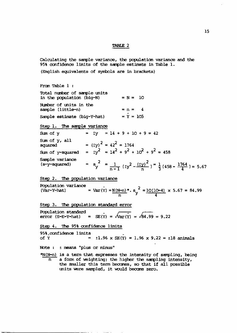
Calculating the sample variance, the population variance and the 95% confidence l imi ts of the sample estimate in Table 1.
(English equivalents of symbols are in brackets)
From Table 1 :
Total number of sanple un i t s in the population (big-N)
Number of un i t s in the sample ( l i t t l e -n )
Step 1. The sample variance
Sum of y = Ey =
Sun of y, a l l squared = ( E ~ ) ~ =
2 Sum of y-squared = Ey =
Sarrple variance ( s-y-squared - - s 2 =
Y
Step 2. The population variance
Population variance (Var-Y-hat ) = ~ a r ( Y ) = N(N-n) *. s = lO(10-4) x 5.67 = 84.99
n Y 4
Step 3. The Dooulatiun standard error
Population standard error (S-E-Y-hat) = SE(Y) = /far0 = . 4.99 = 9.22
Step 4. The 95% confidence l imi t s
95%,confidence l imi t s - of Y
Note :
*N(N-n) n
= 21.96 x SE(Y) = 1.96 x 9.22 = ±1 animals
 means "plus or minus" is a term that expresses the in tens i ty of sampling, being a form of weighting; the higher the sampling intensi ty, the smaller this term becomes, so that i f a l l possible uni t s were sampled, it would become zero.

~n th is -1e t k 95% cmiidence l i m i t s repmsent 17% of the sanple estimate of 105 animals. The precision of this single
estimate can thus be expressed as - Y = 105 217% animals.

SECTION 3 RANDOM NUMBERS, RANDOM SAM>= AND MAPS
3.1 Randan Number Tables
A random number table is a list of single d ig i t s fran 0 to 9
that occur in a to ta l ly unco-ordinated and random order. The two
basic properties of randan ndnber tables are (1) each d ig i t occurs
w i t h the same overall frequency, and (ii) there is no connection
between the occurrence of one d ig i t and the occurrence of a
neighbouring one. Fran this it follows that the dig i t s may be
d i n e d into sets of any length to give random nimbers of any size.
Tables of randan numbers occur in many different shapes and
sizes. To use the randan number tables, f i r s t choose any s tar t ing
point (e.g. page three, row four, calm 2) and then decide w h e t h e r
to go down a w l u m o r along a row. These two decisions must be
made before looking a t the nuirbers. Then, write down the nunbers
fran the table In the order in hi& they occur. These rules must
be followed quite mechanically.
exanple :-
to choose ten randan nwtoers between GO and 99
choose a start ing point in the way described and write
down the f i r s t ten nunbers in the order in which they
occur.
to choose f ive random numbers in the range 35 t o 73
choose a start ing point and write down the nunbers as
they occur, but disregard any that are - less than 35
o r more than 73. - three d ig i t nunbers.
I f three d ig i t nunbers cure required, e.g. in the range
GO to 120, then follow the sane procedures only write
down the dig i t s in groups of three. If going down a
colmn, the pair of d ig i t s in the colum would be grouped
with the f i r s t d ig i t in the neighbouring colum, while
i f going along a rcw the dig i t s are slirply written down
in groups of three. Larger nunbers, e.g. w i t h four o r
five digi ts , can be found in the same way.
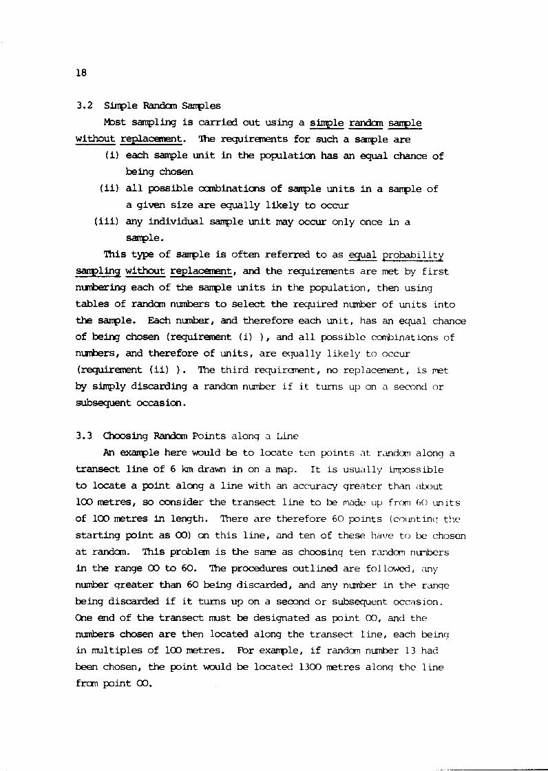
3.2 Simple Randan Sanples
mst samplhg is carried ou t using a smle randan s q l e
w i t h o u t replacement. Ihe requirements f o r such a sample are
(i) each sample u n i t i n the population has an equal chance of
being chosen
(ii) all possible combinations of sample u n i t s i n a sarrple of
a given s i z e are equally l i k e l y to occur
(iii) any individual sample un i t may occur only once in a
sarrple . 'Ibis type of s q l e is often re fe r red to a s equal probability
sanpling without replacement, and the requirements a r e met by f i r s t
numbering each of the sample u n i t s in the population, then using
t a b l e s of randan numbers to select the required number of un i t s i n to
the sanple. Each nLinker, and therefore each un i t , has an equal chance
of being chosen (requirement (i) ) , and a l l possible combinations of
numbers, and therefore of un i t s , a r e equally l i ke ly t o oc:cur
(requirement (ii) ) . The t h i r d requirement, no replacement, is met
by simply discarding a random number i f it turns up on '1 second or
subsequent occasion.
3 . 3 Choosing Randan Points alonq a L i n e
An example here would be to locate ten points a t rmdom alonq a
t ransec t line of 6 krn drawn in on a map. I t is usually L-qmssi-ble
to locate a point along a line with an accuracy qrea te r than about
100 metres, so consider t h e t ransec t l i n e t o be made up from 60 units
of 100 metres in length. There a r e therefore 6 0 points (count 1nq t h e
s t a r t i n g point a s 00) on t h i s line, and ten of t h e s e have to be chosen
a t randan. This problem is the same a s choosinq ten random numbers
i n the range 00 to 60. The procedures out l ined are followed, any
number q rea t e r than 60 beinq discarded, and any number in t h e ranqe
being discarded i f it turns up on a second o r subsequent occasion.
One end of the t ransec t must be designated a s point 03, and t h e
numbers chosen are then located along the t ransect l i n e , each bemq
in multiples of 100 metres. For example, i f random number 13 had
been chosen, the point would be located 1300 metres alonq t h e line
f r an point 00.

3.4 Choosing Randan Points in Space
Fig. 2 shows an oddly shaped area in which it is required to
locate a nunter of random points. Ihe f i r s t step is to set up a
pair of axes a t r ight angles to each other and long enough so that
each covers the whole of the area. These lines form the x-axis
(horizontal) and y-axis (vertical) of a grid co-ordinate system.
Ihe two axes must then be divided into ocnvanient intervals, for
example intervals of 100 metres as in the l a s t example. Tables of
randan nmbrs are nuw used b m s e pairs of ranihn nunbers. The
f i r s t of a pair gives the location of the point along the x-axis
while the second gives the location along the y-axis (Fig. 2). Each
point is plotted on a nap by locating it along the tw axes, being
discarded i f it f a l l s outside the area. Pairs of randan numbers are
drawn unt i l the required nurrber of points have been located within
the area.
3.5 Maps
Maps are necessary for any census work and it is important t o
become well acquainted w i t h the meaning of different map scales.
This is especially important when locating sample units and when
measuring areas. I f an area measured on a 1 : 50,000 scale map is treated as i f it were from a 1 : 250,000 map, an error of times 5
would result, which would lead to sane very curious sample estimates.
The scale of a map relates a distance on the map to a distance
on the ground. A scale of 1 : 250,000 means that one unit measured
on the rasp w i l l represent 250,000 units on the ground. Thus, a
transect of 2 an measured on a 1 : 250,000 map represents
2 times 2 5 0 , 0 0 0 ~ 500,000 anon the ground, 1.e. 5 km. Similarly, a line of 1 km on the ground w i l l be 1/250,000 km = 0.04 km = 4 m on
a map of this scale.
In many Sample Counts the area of a census zone, o r sometimes
the area of each sample unit, has to be known, and this can only be
measured from a map. The best way of doing this is to use an
instrument known as a planimeter which measures area directly when
thelarmloftheinstrumentisrunaroundaboundary. Anareaof
known s ize must f i r s t be marked in on the map by drawing it t o scale

(e.g. a circle w i t h a known radius, or a square w i t h carefully
measured sides). A number of measurements are then made w i t h the
planimeter of this known area, giving a cal ibrat ion of the
instrument fo r t h a t map. A number of measurements a re then made of
the census zone, the average reading from t h e known area being
subsequently used to calculate the area of the census zone.
The procedure fo r measuring the area of a census zone on a
1 : 250,000 map would therefore be as follows :-
carefully draw a scpare w i t h sides of 2 an. This therefore 2 represents an area of 5 x 5 km = 2 5 km on this scale of
map make a number of measurements of the sides of this square
w i t h the planimter , recording each measurement as it is
taken. Take the average of these measurements and c a l l it
A.
similarly make a number of measurements of the census zone
w i t h the planJJneter, take their average, and call it a ' . 2 since A uni ts measured on the planimeter represent 25 km ,
the area of the census zone is found by
repeat steps (a) through (dl two more times, and average a l l
the results. I f a planimeter is not available there are a nunber of more o r
less accurate alternatives. One method is t o make a number of tracings
of the census zone on paper of the same thickness. Alongside each
tracing a square of known area is drawn in. This square, and the
census zone, are then very careful ly cut out and weighed on a f ine
balance. The area of the census zone can then be found from the
average weights of the square of h a m area. Thus :
let W be the average weight of a square of known area, A km 2
w' be the average weight of the census zone 2 then, area of census zone = A . w'km
w

Fig. 2 Choosing random points in space
x - a x i s
10 2 0 3 0 4 0 5 0 6 0 7 0
- - - Â ¥ 1 ^
I - - - - - - - - - - - - - I
o f z o n e
( 7 )
The x-axis and y-axis have been divided i n t o units of 100 metres. The
two axes are a t r ight angles t o each other and cover the whole of the
census zone (so l id boundary). Pairs of random numbers are chosen and
the points are located along the two axes.
random numbers Point x-axis y-axis
19 f a l l s inside 5 2 outside 4 5 inside 3 8 outside 2 8 inside 7 5 outside 5 2 outside 86 outs ide 2 0 inside
the zone and is included excluded included excluded included excluded excluded excluded included

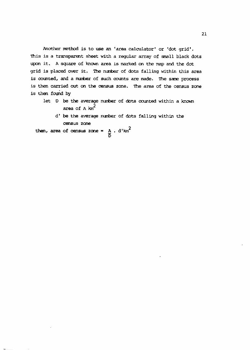
Another method is to use an 'area calculator' o r 'dot gr id ' .
This is a transparent sheet w i t h a regular array of small black dots
upon it. A square of known area is narked on the nap and the dot
grid is placed over it. The number of dots fal l ing within t h i s area
is counted, and a number of such counts are made. The same process
is then carried out on the census zone. The area of the census zone
is then f& by
let D be the average number of dots counted within a known
area of A km 2
d ' be the average number of dots falling w i t h i n the
census zone
then, area of census zone = - A . d'km2 D

SECTION 4 METHODS OF AERIAL SAMPLE COUNTING
4 .1 Introduction
Aerial sample counting is now a very frequently used method of
counting large mamnals. The next six Sections are devoted to various
aspects of the methodology. It is however, Ijnnportant to realise that
the principles outlined here apply equally well to other methods of
sanple counting, either fran vehicles, on foot, o r by indirect
methods (e.g. spoor counts, pellet counts, capture-recapture methods).
4.2 Aerial Transect Sampling
The aerial transect nethod is the roost popular type of sampling
method employed. The principle is that the a i rc ra f t f l i e s in a
straight line fran one side of the census zone to the other a t a
fixed height above the ground. Streamers are attached t o the wing
struts of the a i rc ra f t so that the observer sees a s t r i p demarcated
on the ground. The w i d t h of the s t r i p can be decided in advance and
the streamers positioned so that the desired w i d t h is obtained
(Section 5) . The transects are the sanple units, and the observer
counts a l l the animals that he sees between the streamers.
The sample units are located by drawing in a base-line on a map
of the census zone (Fig. 3). This base-line is divided into sections
of the same length as the width of the chosen transect s t r ip . I f , for example, a 300 met re s t r i p is being used, then a 60 tan base-line
would be divided into 60/0.3 = 200 units. The required number of
transects are then located by choosing random nurrbers in the range
00 to 200 and locating these points along the base-line. The
transacts are then run through these points a t r ight angles to the
base-line, the line of each transect being drawn in on the map to
aid navigation.
The base-line must be made long enough so that transects passing
through it can 'cover' a l l parts of the census zone. The x-y base-line in Fig. 3 could not be used, for large portions of the
census zone could not be crossed by transects. I f it was necessary
to have the transects in this particular orientation then the
base-line would have t o be extended to x' -- y'. Of course, only

Fig. 3 Locating the transects along a base-line for aer ia l
transect sampling.
boundary o f
census zone
the base-line A - - - B is made long enough so that it covers the whole area of the census zone. Random points are located along it, and the transects pass through these
A
points a t right angles t o the base-line. The transects pass from one side of the census zone t o the other. All animals seen w i t h i n the demarcated s t r i p are counted.
I t r a n s e c t s
t h i s base-line x --- y would not be long enough for some*- areas of the census zone could not have a transect \ passing through them. The . extended" line x' --- y t would be long enough.
boundary o f
c e n s u s z o n e
i n very oddly shaped census zones the transects may be outside the zone for some of t he i r length (dotted portions). Animals are only counted along those parts of the transects that l i e within the census zone (solid portions)


those portions of the transects passing through the census zone
would be flown along. Similarly, the base-line most not be so long
that transects can pass outside the census zone.
The transects can a l l be of different lengths i f necessary, and
it is in fact rare to find a census zone that does not d ic ta te
transects of different lengths. In the oddly shaped census zones
(e.g. Fig. 3) the transects may even pass out of the zone and then
into it again. In this case the a i rcraf t has to f l y along the whole
length of the transect, but animals are only counted within the
census zone.
The two main characteristics of aer ia l transect saxrpling are
therefore (i) the transects are parallel t o each other and cross the
census zone at randan points along a base-line, and (ii) the aircraf t
f l i e s once down each transect line and the observers count a l l
animals seen between the streamers. Examples of transect counts are
given In various publications 3,38,41,49
4.3 Aerial Quadrat Sanpling
Quadrat sanpling is much used in the United States of America
but does not seem to have received much attention in Africa. The
sanpling units are quadrats , e.g. rectangles , that are located in
sane suitably random fashion w i t h i n the census zone. Most usually
the quadrats are square in shape l 8 , although rectangular shaped
quadrats have been used2. The procedure used by most authors is t o
divide the whole census zone into grid squares of appropriate size
(e .g. 2 x 2 miles, o r 1 x 1 mile) and select sane of these grid
squares to search. The selection is most simply done by numbering
the squares from 01 to N, then choosing the necessary number of
random numbers in t h i s range. A s l ightly different method has been
employed whereby quadrats have been constructed from random points 22 located in space .
Once the selected quadrats are marked in on a map of the census
zone, the aircraf t v i s i t s each one in turn and locates and counts
every animal within them. The a i rcraf t can spend as long as is
necessary in counting each quadrat.

4.4 Aerial Block Sanding Block -ling is veq shllar to quadrat -ling except that
the sairple units are blocks that are demarcated by physical features
present on the ground (e.g. rivers and streams, roads and tracks,
h i l l s , ridge tope, edges of woods etc.). A sanple of blocks is
chosen by locating randan points in space, then counting those blocks
in which a randan point fa l ls . Alternatively, the blocks can be
nuttered fron 01 to N and the required nurber of randan nuiters drawn.
Although the use of blocks as sanpling units is sometimes
mentioned in passing27 it is surprising to find that they have never been used in practice for an aerial sample count. They are often
used in total aerial counts (Section 9), and they are often used in
ground sample counts (Section 10) , and they are sonetlnes used as a
method of checking the accuracy of transect counts3. This is
supr is lng, for blocks have m y advantages over quadrats as -ling
units (see below).
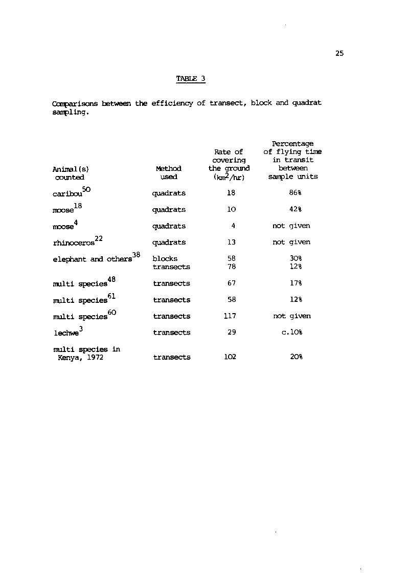
4.5 Conpariscns Between the Three Methods
(i) Costs
Wansects ham the great advantage over blocks o r quadrats
in that the a i rc ra f t is operating a t maximum efficiency when flying
in a straight line. This shows in two ways (Table 3). First ly, the
a i rc ra f t never retraces its track o r backtracks and consequently the
rate a t which the ground is covered is higher than for blocks o r
quadrats. Secondly, as the transects are parallel to each other, and as the transects usually tend to be near to each other, the
proportion of "dead time' (i.e. the tine spent by the a i rc ra f t in
travelling from one sample unit to another) is low. ( ii) Navigation
Navigation is considerably easier with transacts, for the
pi lo t has only to follow a straight line on a map and then need only
locate the start ing point of the next straight line. Both blocks
and quadrats have to be seamhed for and the boundaries identified
precisely. This is often extremely d i f f icu l t to do, especially with
quadrats locatxd in featureless camtry. With no msical mark on
the ground, it is often impossible to decide exactly where the
quadrat s ~ d be18 and this can only lead to m r s that are
2 5
TABLE 3
Ccrrparisons between the efficiency of transect, block and quadrat
Animal (s) counted
caribou50
moose 18
moose 4
rhinocerosz2
elephant and others38
mlti species 4 8
mlti species 61
multi species in Kenya, 1972
Method used
quadrats
quadrats
quadrats
quadrats
blocks transects
transects
transects
transects
transects
transacts
Percentage of flying time in transit between
sairple units
not qiven
not given
not given

impossible to gauge.
(iii) Boundary effects
All three methods suffer from boundary effects to some
extent in that it is always difficult to decide whether or not an
animal is inside or outside the sample unit. In transect counting
the rule is that the observers count any animals seen within the
streamers whatever the aircraft happens t o be doing. It is
imnediately apparent that the width of the demarcated s t r ip depends
upon the pilot maintaining s t r i c t height control and strict bank
control. In Section 6 methods for doing this are discussed in some
detail. Noretheless, the observer does have a physical mark in the
form of the streamer to indicate whether or not an animal should be
counted. In quadrat sanplinq th is problem is very acute for there
is no physical mark of any kind by which the observer can make th i s
decision. This again can only lead to errors whose magnitude it is
impossible t o gauge. The situation is better with block counting for
the boundaries of the blocks are made up from physical features,
ensuring simplicity in deciding whether or not an animal is inside
the block. However, many 'natural' boundaries (e.g. rivers and
streams) tend also to be habitat edges across which there is often
considerable movement.
(iv) Counting
The great disadvantage of the transect method is that the
observers have only one chance t o locate and count groups or
individuals because the aircraft makes only a single pass along each
transect line. In block or quadrat sanpling the aircraft can make
as many passes as required in order to locate and count a l l groups.
There are disadvantages in that great care must be taken t o avoid
double counting and to ensure that all the area is indeed searched.
These problems are also considered in Section 6.
Unfortunately there are no w e l l controlled experiments In
which block or quadrat sanpling have been tested against transect
sapling. Seme authors have attempted it but In such a way that the results appear meaningless. For example, In one study a camparison
was made between the density of noose counted in intensively searched
1 x 1 mile quadrats with the density found when counting a transect
s t r ip of '5 mile. As a s t r i p width greater than \ mile is normally
far too wide for effective counting (but see pp. 30 and 4 0 ) , it was
not surprising to find that the transect densities were considerably
lower than the quadrat densities. In one study where block counts
were used as a check against transect counts, the results were not
found to be s tat is t ical ly different, even though the blocks were 38 being searched more intensively . In th is case both counts were
being carried out in a sensible fashion.
There are certain conditions under which the transect method
does not work a t a l l well. For example, when the ground is very
broken and when there are many gullies and rocky outcrops; or,
of course, when the vegetation becones very thick; or when the
country is very mountainous. In the f i r s t two cases animals can only
be located by intensive criss-crossing and 'buzzing' with the
aircraft. In the las t case (very mountainous country) the problems
of height control make the transect method ineffective.
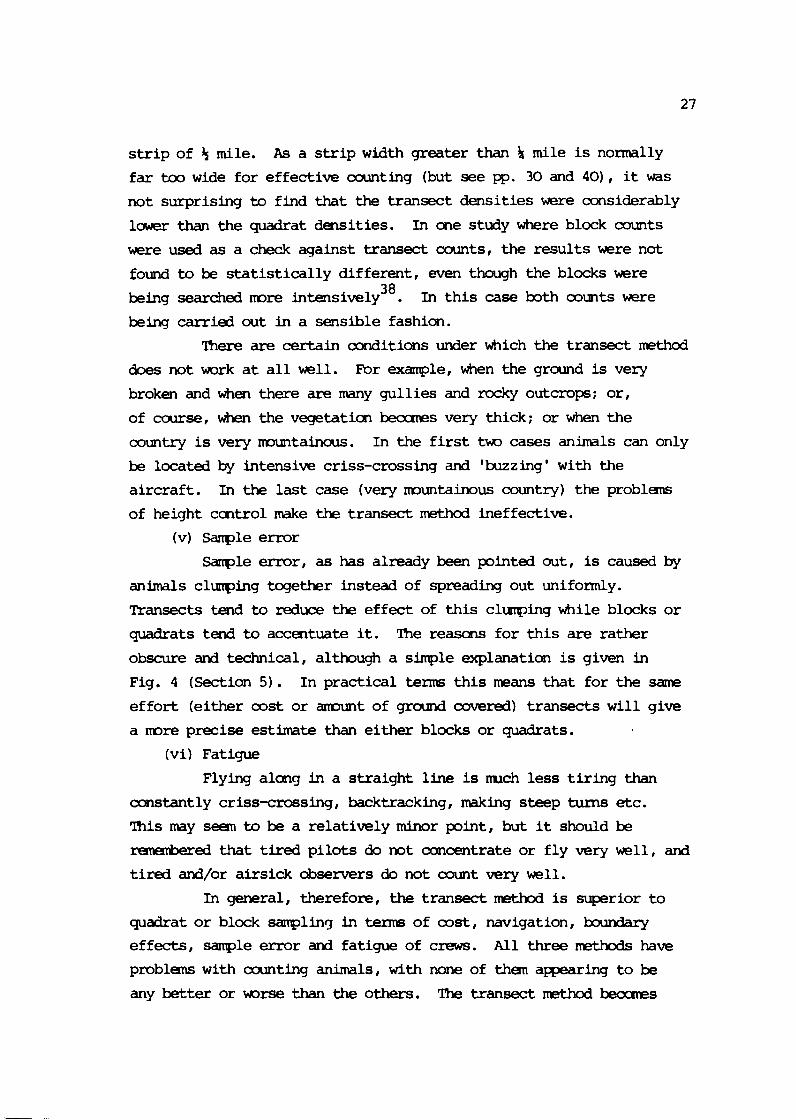
(v) Sanple error
Sample error, as has already been pointed out, is caused by
animals clunping together instead of spreading out uniformly.
Transacts bend to reduce the effect of this clunping while blocks or
quadrats tend to accentuate it. The reasons for this are rather
obscure and technical, although a sirnple explanation is given in
Fig. 4 (Section 5 ) . In practical terms this means that for the same
effort (either cost or anount of ground covered) transects will give
a more precise estimate than either blocks or quadrats.
(vi) Fatigue
Flying along in a straight line is nuch less t i r ing than
constantly criss-crossing, backtracking, making steep turns etc.
This may seem to be a relatively minor point, but it should be
remarbered that tired pilots do not concentrate or f ly very w e l l , and
t ired and/or airsick observers do not count very wel l .
In general, therefore, the transect method is superior t o
quadrat or block sanplinq in terms of cost, navigation, boundary
effects, sample error and fatigue of crews. All three methods have
problems w i t h counting animals, with none of them appearing t o be
any better or worse than the others. The transect method becomes

ineffective in very broken country, when the vegetation is very thick
and/or patchy, and when the country is very mountainous. In these
cases some form of block sampling wuld be preferable to quadrat
sanpling because of the advantages over boundary effects.
SECTION 5 DESIGNING AN AERIAL SAMPLE COUNT
5.1 Introduction
Although there are theoretically many different ways to design
an aerial sanple count, practical considerations fortunately limit
the options to a few well tried and trusted methods. This Section
considers sane of the more important factors in a reasonably logical sequence from a very practical viewpoint. First, the census zone
roust be defined, which in some situations is not particularly easy to
do; then the 'best ' method must be chosen; next sarnple error must be
considered, and it will be seen that there are some sinple techniques for reducing sample error at the design stage without increasing the
costs of the census; then, the sources of bias and errors must be
identified and steps taken to minimise them; finally costs mist be
taken into account. It is not possible to say which of these is the
most important, for this will vary from area to area, from animal to
animal, and will also depend upon resources. For example, a
biologist might be given unlimited funds to obtain an estimate with
95% confidence limits of not more than 10% of the estimate. His
approach, in this fortunate position, would be very different from
that in which he had been allocated a certain amount of money and
told to do 'the best he couldt.
5.2 Def ining the Census Zone
The census zone, already defined on page 9, is the area within which you wish to estimate the nu* of anlmals. If this happens to
be a defined area such as a National Park, a Game Reserve or a study
area then the boundaries of the m s u s zone are sinply those of the
particular area. If, on the other hand, the objective is to estimate
the number of animals in a certain population, then the census zone
must be defined by the area occupied by that population at the time
that the census is carried out. This requires quite detailed
knowledge of the movements and distribution of the population
concerned, otherwise serious errors could result. Examples of how
to use this type of information to define the census zone are
available ' . 1n ~erengeti , for exanple, the problem was to
estimate the number of animals in the migratory wildebeest population37. This population moves over a vast area in the course
of a year but at any one time occupies only a small fraction of the total area. Systematic surveys were used to locate the population on the basis of which information it was possible to define a census
zme that mtained all the animals.
The size of the census zone mast be kept within reasonable
limits otherwise the census becanes unmanageable. It has been our 2 experience that 10,000 km is about the largest area that can be
reasonably treated as a single zone, and areas larger than this
should be split up in sane way and sampled as separate entities.
This is one application of what is known as stratification, which
will be dealt with in more detail in Section 5.4.
5.3 Choosing a Sanpling Method
The decision to be rode here is between transect s w i n g and
block sanpling, quadrats being ignored because of the difficulties of
locating the lmmdaries m the ground. Xhe relative advantages of
these two methods have already been discussed in the previous
M m . Fbr the masons given there, and for additional masaw
given later in t h i s Section, transect sampling should always be used
except in the following situations :-
(a) If the animals occur in very large and conspicuous herds (e.g. buffalo) block ~cnrpling - or perhaps even total counting - is preferable because a very wide searching strip can be used. Fbr
exanple, in block counts of buffalo in open savannah woodlands, the
ground can be covered at a rate of 240 km2 per hour using a strip of
about 1.5 km in width. This is a much higher rate of ground coverage than with transact sampling, and it is only possible because the
observers have to search for and locate large herds rather than
individual animals. Cnce a herd is located the aircraft can divert
to the herd in order to count it.
(b) If the country is very broken (e.g. with many rocky outcrops or ravines) or if the vegetation is very thick and/or patchy, block
counting is preferable because these difficult areas can be searched
particularly intensively.

(c) If the country is really mountainous, w i t h precipitous valleys and high mountain walls, transact sampling is downright dangerous. It is sheer madness to try too f l y a l ight a i rc ra f t in a straight line close t o the ground under these conditions. In
&tion, t b inewitable massive var ia t ims in flying height over this sort of country would produce unacceptably large biases that
would be d i f f icu l t too correct for. Block oounting would have to be
used instead.
5.4 Reducing Sairple Error The main cause of s a p l i n g error is related to animals not being
evenly distributed over an area. This means that the sample units w i l l tend to have different numbers of animals in them, chance thus
selecting a set of units into a sanple that wi l l give one population estimate out of a whole range of possible population estimates.
Sarrpling error is more aggravated the more bunched - o r aggravated - the animals axe, for this leads to a bigger variance between the numbers found In each unit. SarrplIng error can only be reduced by
minimising the effect of this clumping. The strategy, therefore, is
to create a t the outset - 1.e. a t the census design stage - a
population of sample units that has as low a variance as possible. All the points mentioned below are discussed in great detail in
general - Ut66 . (1) the shape and s ize of sanpllng unit
Sane types of sampling units wi l l always give a higher
variance, and therefore higher sanpllng error, than others. Fig. 4
shows a census zone which has been divided up into sixteen transects and sixteen quadrats each of the sam size. Each dot in Fig. 4
mpmsents t h 1ocatia-i of an animalt and it l a hmdla t e ly obvious that the quadrats have an 'all-or-nothing' ef fect t i.e. they ei ther contain many animals o r none, while the transects a l l tend to have
roughly the same nmrber of animals in them. The population of quadrats is therefore more variable than the population of transects,
and smple error w i l l therefore be higher with the quadrats than with the transacts. This is also shown in Fig. 4. The variance of the
quadrats (43) is very much higher than the variance of the
transects (8 ) , and the effect of this on sample error is demonstrated
by the results of three randan samples of 25%, 50% and 75% of the
sanple units. The 95% confidence l imits of the transects are always
less than those of the quadrats.
A population of blocks w i l l , i f anything, intensify the
aggregations of animals, blocks thus tending to have an even higher
variance than quadrats. This demonstrates the great advantage of the
transect method of sarrpling, for transects have an inherently low
sampling error.
The reason for this is sl ightly obscure but can be explained
as iollows. Fach of the quadrats in Fig. 4 only collects infomat img
about the density of animals in a small, localised part of the census
zone. In contrast, each of the transects collects 'informationg
across the whole census zone. It is obvious that the more information
you have about a census zone the less room there is for error.
Accordingly, since transacts collect more information than quadrats, they nust la to a smaller smpling error.
One general rule of sanple theory is that for a fixed amount - of material to be sampled, a lower sanpling error wil l be achieved i f
many small units are counted rather than a few larger ones. In other words, 50 blocks of one square kilometre each w i l l give lower
confidence l imits than w i l l 25 blocks of two square kilometres. This
follows frun the previous paragraph, for the f i f t y small blocks w i l l
collect much more information than the twenty-five larger ones, and
therefore sarnple error can but only be smaller. Unfortunately it is
not always possible to follow this advice because many small sample
units are inordinately expensive to count while fewer and larger units
cost much less. For fixed costs, therefore, a lower sample error w i l l be achieved by counting laryer units than smaller units.
Although this may seem to contradict the f i r s t statement in this
paragraph, on close examination it w i l l be seen to be a logical
cmseqw~ce of it. Sane capmnise must therefore be reached the s ize of unit, the nurrber to count, and the costs of counting each
one. Publications are available which Indicate ways and means of
doing this 13,66 . However, in aerial sampling, practical amsideraticms in t e r m s of maximising the efficiency of the aircraf t

Fig. 4 The effect of different shapes of sampling unit on sample error. A census zone has been divided up into 16 equal sized sampling units, either transects or quadrats.
95% confidence limits from samples of different sizes
2 size of sample s Y
25% 50% 75%
transects 8 59% 48% 34%
quadrats 43 136% 112% 78%

and the observers outweigh statistical considerations leaving
relatively little roan for manoeuvre.
With block or quadrat sq1i.m~ it is mtoefficient to have
the unit of a size that can be counted in one flight of two to three
hours duration. Reducing the size of the unit has a very dramatic
effect on costs. The amount of dead time, i.e. time spent fly-
from one unit to the next, becomes very high, and the amount of time
spent locating the boundaries is proportionally higher with mller
units than with larger ones. An extreme case of the expense of
counting very small units is given by an unsuccessful census of
gazelle in the Serengeti. The idea was to take a large number of
photographs of gazelle at randan locations across the Serengeti
Plains. Sane 600 photographs were taken, in about ten hours flying.
Since each exposure was taken at a 1/1000 sec., the aircraft was
collecting information for about half of one second during the entire
ten hours flying. This is not an efficient method of using an
aircraft.
In transect sanding there is more freedap of choice. Theoretically, the size of the unit can be altered by altering the
strip width, but here considerations of counting bias are more
tirportant, and the strip width should always be chosen to minimise
this source of bias (see 5.5 below). However, the size of the unit
can be altered by alterm the length of the transect. In a
rectangular census zone, a lower sanple error will be achieved for
the same amount of flying by running the transacts across the shorter
dimension. In this way the same amount of material will be sanpled
in m y small units rather than fewer larger ones. Of interest here
is the fact that the costs will be exactly the same, another advantage
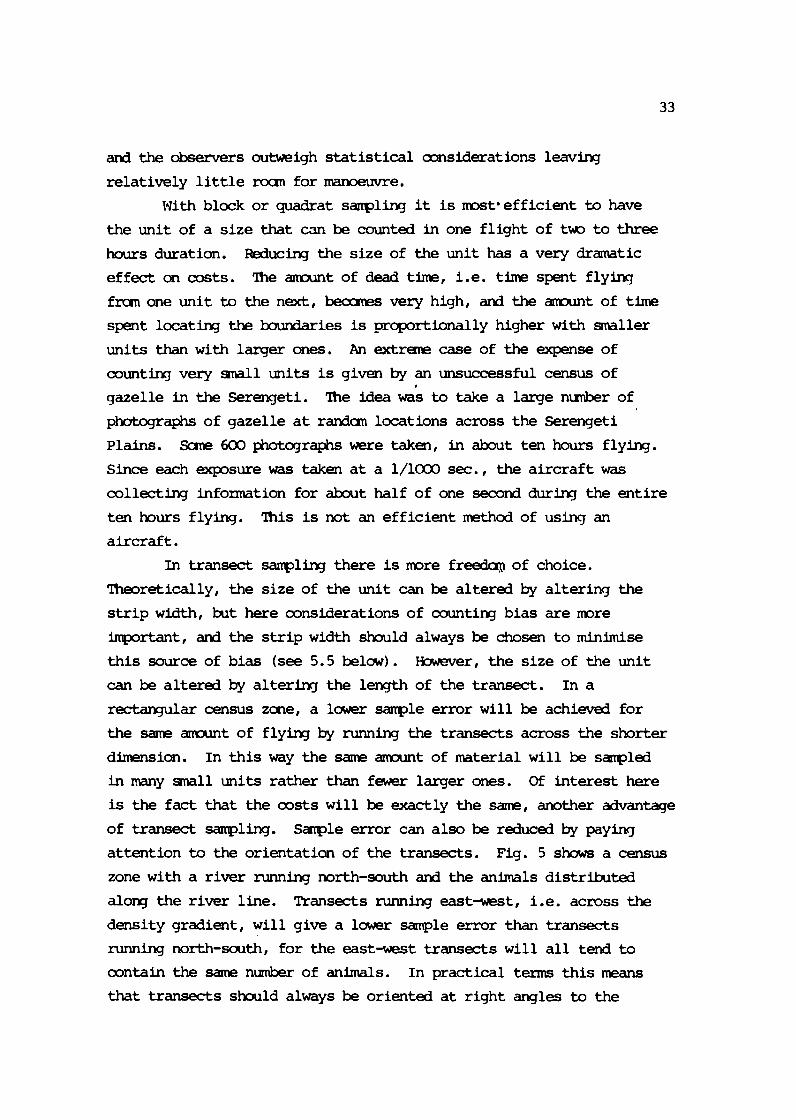
of transect sampling. Sanple error can also be reduced by paying
attention to the orientation of the transects. Fig. 5 shows a census
zone with a river running north-south and the animals distributed
along the river line. Transects running east-west, i.e. across the
density gradient, will give a lower sample error than transects
running north-south, for the east-west transects will all tend to
contain the same number of animals. In practical terms this means
that transects should always be oriented at right angles to the
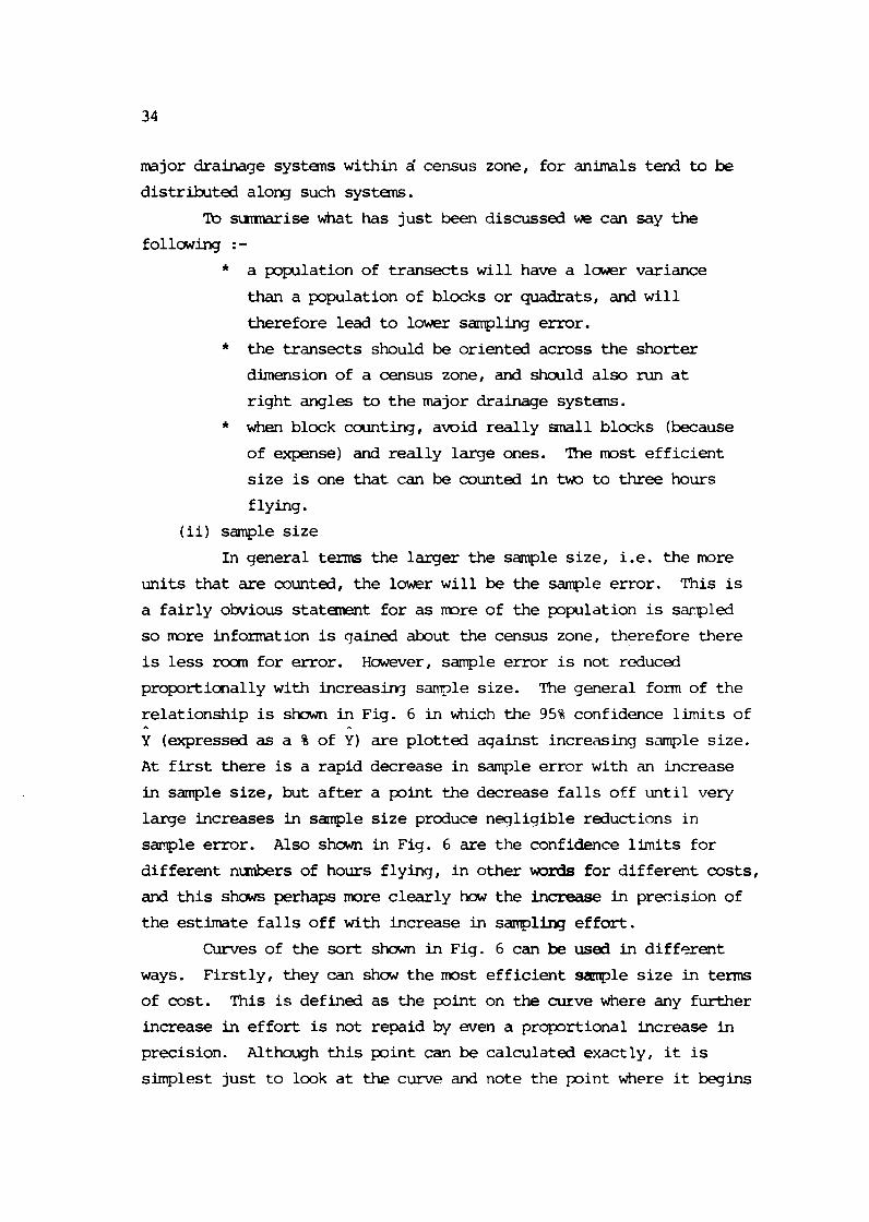
major drainage systems w i t h i n zi census zone, f o r animals tend too be
d is t r ibu ted along such systems.
To sumnarise what has j u s t been discussed we can say the
following :- * a population of t ransec ts w i l l have a lower variance
than a population of blocks o r quadrats, and w i l l
therefore lead t o lower sampling error.
* the t ransec ts should be or iented across the shor te r
dimension of a census zone, and should a l s o run a t
r i g h t angles to t h e major drainage systems.
* when block counting, avoid r e a l l y s n a i l blocks (because
of expense) and r e a l l y la rge ones. The roost e f f i c i e n t
s i z e is one t h a t can be counted i n two to three hours
f lying.
(ii) sample s i z e
In general terms the larger the sample s i z e , i.e. the more
un i t s that are counted, the lower w i l l be the sample error. This is
a f a i r l y obvious s ta tanent f o r a s more of the population is sanpled
s o more information is qained about the census zone, therefore there
is less roam f o r error. However, sample error is not reduced
proportionally w i t h increasirq s a i l e s ize . The general form of t h e
re la t ionsh ip is shown in Fig. 6 in which the 95% confidence l imi t s of ,. ,. Y (expressed as a 3 of Y) are plot ted aqainst increasing sample s i ze .
A t f i r s t there is a rapid decrease i n sample e r r o r with an increase
in sample s i ze , but a f t e r a point the decrease f a l l s o f f u n t i l very
large increases in sample s i z e produce neql iqible reductions i n
sample error. Also shown in Fig. 6 are t he confidence l imi t s f o r
d i f f e r en t nunbers of hours f lying, i n other words f o r d i f f e r en t costs,
and this shews perhaps more c l ea r ly how the increase in precision of
t h e e s t h t e f a l l s o f f w i t h increase in sampling e f f o r t .
Curves of the sort shown in Fig. 6 can be used in d i f f e r en t
ways. F i r s t l y , they can show t h e most e f f i c i e n t sample s i z e in terms
of cost . This is defined a s the point on t h e cuxve where any fur ther
increase in e f f o r t is not repaid by w e n a proportional increase in
precision. Although this point can be calculated exactly, it is
simplest jus t to look a t the curve and note t h e p o i n t where it begins
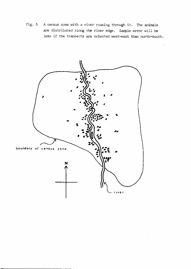
Fig. 5 A census zone with a r i v e r running through it. The animals
are d i s t r i b u t e d along t h e r i v e r edge. Sample error w i l l be
less i f t h e t r a n s e c t s are or ien ted west-east than north-south.

Fig. The rela t ionship between the '+ precision of an estimate (expressed
as 95% confidence l imi t s as a % of I? ,5 h the estimate) and increasing sample 0 4-1
s i z e . 'X' marks the point of
maximum sampling eff ic iency. 3 Le h
1-1 14-1
$
.r^ 1-1 h
4-1

to ' f l a t t e n ou t ' . I n Fig. 6 this point is marked by 'XI,
representing about 52 transects costing some 19 hours f lying, w h i c h
w i l l g ive an estimate w i t h a precision of about 21%. Alternatively,
Fig. 6 could be used to f ind out how many t ransec ts , and how much
cost, w i l l be required f o r any stated precision, or conversely what
the precision is l i k e l y to be f o r any given cost. Curves like this
are r e a l l y very useful.
Fig. 6 was constructed from data obtained during an aerial
t ransec t count of elephant in Ruaha National Park, Tanzania. It was
used to decide how many t r ansec t s
constructed in the following way.
95% confidence l i m i t s of
to f l y in a subsequent census being
From Table 2 we see that A
Y = 1.96 x SE(Y)
= 1.96 x /VarfYI
Knowing N and s , the curve is calculated by subs t i tu t ing d i f f e r e n t
values of n i n the equation, and then p lo t t i ng the 9 5 % confidence
l i m i t s (expressed a s a % of Y) against n. This is f i n e so long a s
you have an estimate of s f but it be-s s l i g h t l y t r i cky i f you do .i
not. Two ways around t h i s a r e to (a ) go out and count a few
transects in order to get a rowh estimate of s ( t h i s could be done Y
as part of an observer t ra in ing prcgranroe), or (b) use da ta published
from d i f f e r en t areas where the densi ty of animals is roughly the same
as in your area. N is simple t o calculate . For t ransec t counting it
is found by dividing the length of the base-line by the s t r i p width,
while w i t h block counting it is simply the nunber of blocks into
which the census zone has been divided. 2 The ac tua l shape of the curve w i l l depend upon s . I f this
Y is small then t h e increase i n the precision of the estimate increases
very rapidly w i t h increasing sample s i ze , then f a l l s o f f very
rapidly. I f s is large, then the increase in precision is less Y
marked, and there is a less marked f a l l o f f .
I f absolutely no information can be obtained about an area
before a census, then as a general r u l e of thumb avoid very small
samples (less than ten) and very large samples (more than f i f t y ) .

It is always important to ranarber that sample error is not reduced
by the percentage of units that are sampled but by the number of
units that are sampled. It is often instructive to carry out the
calculations mentioned above on data given in published accounts of
censuses. In one recent, and nameless, paper the authors were
obviously extremely proud at having put in a great deal of effort
and expense to count a large number of transects. I calculated that
with exactly one half of the effort the precision of their final
estimate would have been only 3% less. To my mind they wasted a lot
of money.
( iii) stratification
TITS principle of stratification is to divide a census zone
into sub-zones, or strata, in which the density of animals is
approximately uniform. Independent samples are then taken within
each of the strata, the results beinq combined later. In.Fiq. 7 a
census zone is shown in which there are very obvious differences in
animal density. If sampled as a single zone the population of sample
units would have a very high variance and therefore sample error
would also be high. By dividinq it, as shewn, into three strata on
the basis of density, each stratum is more uniform within itself than
is the whole census zone. TTie population of sanple units within each
stratum will therefore have a low variance, and the overall samplinq
error will bte reduced.
The problem now is to allocate the sampling effort between the
strata. In general terms a stratum with a high variance should
receive more sampling effort than a stratum with a low variance.
Since the variance within a stratum will be directly proportional to
the density of the animals in the stratum, sampling effort should be
allocated an the basis of animal density. This procedure is shown in
Fig. 7 where the densities in each stratum are taken to be 10, 5 and 2 1/km respectively. Sampling effort would thus be allocated in the
ratios 10/16, 5/16 and 1/16, i.e. 62.5%, 31.25% and 6.25% respectively.
Once the samplinq effort has been allocated then completely
independent samples must be drawn within each of the strata. When
transect sampling, this will entail constructing a different base-line
within each stratun, while with block samplinq different sets of

Fig. 7 The principle of s t r a t i f i ca t ion on the basis of differences
i n animal densi t ies
 0 a m - * *à 0
0 9 - - - - - - - L a
Stratum A
density circa 1 0 / h 2
Stratum B
density c i rca 5 / h 2
Stratum C
density c i rca 1/h 2
If 20 hours flying were available f o r a census, it would be
allocated between the three s t r a t a as follows :
Stratum A would be allocated 20 x 10/16 = 12.5 hours
StratumB I I 1 1 2 0 x 5/16 = 6.25
StratumC I ' 11 I I 2 0 x 1/16 = 1.25 I T


random nunbers would be used to choose the blocks in each stratum.
Examples of stratification can be found in several
publications It is a - -fil for
reducing sampling error at the design stage of a census. However,
good information must be available on the distribution and density
of animals before the stratification can be made, for sample
error can be greatly increased if a mistake is made in drawling the
stratum boundaries. Stratification should be used with caution until
sane experience with census work has been obtained.
Stratification may also have to be used in order to divide a
census zone into units of manageable size. In this case there may be
no reason to suppose that there are major differences in animal
density between the strata, and accordingly the sanpling effort is
allocated in proportion to the area of each stratum. Thus, a stratum
that represented 38% of the original census zone would be allocated
38% of the sampling effort.
A stratum may itself be split up into two o r more pieces. In
Fig. 8 the high density stratun lies on either side of the low
density stratun. The allocation of sanpling effort would now be in
two parts. First, sampling effort is allocated on the basis of
density, the high density having 10/15ths and the low density 5/15ths
of the sampling effort. Secondly, the sampling effort allocated to
the high density stratum is now apportioned to each piece of it in
proportion to its area.
5.5 Avoiding Biases and Errors
If a pilot is maintaining height control by reference to a radar
altimeter he will sometimes be a bit too high, and sometimes a bit
too low, but on average he will be at the required height. This is
known as an error, for the times he is too high are compensated for
by the times he is too low. The same applies to animals moving around
in a census zone. The number moving into a transect strip will be
balanced, on average, by those moving out. A bias, on the other hand,
is an error in a amstant direction. If the radar altimeter was
overloading, so the pilot was always lower than he thought, then
although he would be oscillating around the indicated height he would

always be too low. Here, there would be a negative, or downwards,
bids in his height control. Similarly, if animals are flushed out of
the transect strip by the auproach of the aircraft there will also be
a negative bias in the number of animals counted. In both these
examples the total numbers of animals would be underestimated.
The importance of a bias is that it produces a consistent
inaccuracy irrespective of the sampling design and how much care is
taken over the census. If the radar altimeter, urhum to the pilot, is reading wrongly, the results of the census will be biased, however
much trouble is taken over navigation and counting.
There are three cornon-sense rules that apply to biases :
(a) be aware of the potential sources of bids and take all
precautions to minimise than
(b) design the census in such a way that the most potent sources
of bias can be measured and then corrected
(c) do everything possible to keep the biases constant from
count to count.
i ) biases from the sample design
So long as the sample units are set up in the ways described,
and the sample is drawn completely randomly, no biases should occur
from the sample design.
(ii) biases from the census design
Before the census: The time of year that the census is
carried out must be carefully considered. Animals may move in or out
of the census zone at different seasons. Sane species are also mre
conspicuous at some times of the year than others. Some species
aggregate into larger groups at certain times of the year, thus
increasing sample error. The time of day is also important, for
animals tend to seek shade around midday making them difficult to
count.
Biases from boundary effects should also be considered here.
One difficult aspect of any aerial counting is to decide whether an
individual or a group of individuals is in or out of the sample unit.
It is likely that observers will tend to give the animals the benefit
of the doubt and to include them where possible. With some types of units (blocks or quadrats) this decision is much harder to make than

Fig . 8 A l l o c a t i o n of sampling effort on b a s i s of d e n s i t y and area
for a s p l i t s t r a t u m
The a l l o c a t i o n of 20 hour s f l y i n g would be as fo l lows :
( i ) on b a s i s of d e n s i t y
s t r a t u m A is a l l o c a t e d 20 x 10/15 = 13.33 hours s t r a t u m B is a l l o c a t e d 20 x 5/15 = 6.67 hours
( i i ) w i t h i n s t r a t u m A on b a s i s of area
area of s t r a t u m A, = 420 ton2
areaof s t r a t u m A 2 = 130km2 ) total area of s t r a t u m A = 550 km2
s t r a t u m A, is a l l o c a t e d 13.33 x 420/550 = 10.18 hours
s t r a t u m A2 is a l l o c a t e d 13.33 x 130/550 = 3.15 hour s


with others (transacts). This has already been discussed in Section
4 and will be treated again in the next Section. However, the size
of the unit is iqortant here, for the smaller the unit the larger
will be the proportion of animals falling on the boundary. Larger units therefore tend to reduce this source of bias. A slightly
different example canes from a census of black rhinoceros 22 lh
s q l e units =re rectangular m a t s defined by a fixed strip width
and a fixed length. The length of each quadrat was 'measured' by
flying the aircraft in a straight line for twelve minutes, assuming a
ground speed of 90 mph. There is obviously a potentially large source
of bias here. Firstly, no 'Super Cub' (the aircraft used in this
census) that I have ever met has ever managed to fly with a ground
speed of 90 mph, at least not consistently. Secondly, no precautions
were apparently taken to check the ground speed, or even to check the
direction and strength of the wind during the census. It is
therefore very probable that there was an underestimation.
During the Census : Errors in navigation are unlikely to
produce biases unless, for example, the pilot mistakes one river for
another - or something like that - and consistently stops counting in the wrong place. In block or quadrat sanpling there is a large
potential for bias 'in that the crew may not count the whole area - although methods for avoiding this are discussed in the next Section.
In aerial transect sanplinq height control is the most potent source
of bias, but fortunately precautions can also be taken to correct it.
After the Census : Biases could be caused by consistent
Inaccuracies in measuring distances and areas (through getting the
map scale wrong), but ocmnon-sense, and repeating all measurements a
number of times, should keep this to the miniman.
(iii) counting bias
This is the most potent source of bias in any form of aerial
censuso. Methods for minimising it are discussed in the next
Section, but at the census design stage much can also be done. To
start with, the observers should be thoroughly trained in all aspects
of census work, including spotting and counting animals. Secondly, photography should be used whenever large numbers of anhals are
encountered.

In block o r quadrat sanpling the observers should also be
thoroughly familiar w i t h the methods of assuring that a l l parts of
the sample unit are searched and that none are searched twice (see
next Section).
In aer ia l transact sanpling the most important considerations
are those of flying height, s t r i p width and flying speed, for these
all affect the abi l i ty of observers to count animals.
Flying Height : More animals are missed the higher the
a i rc ra f t is above the 9roind4. lower heights are therefore
preferable unless there is seme good reason for flying higher, e .g . i f the animals run away f m the aircraf t . Ttie most useful height for
transact flying has been found to be about 300 f t . above the ground.
A lower height should be used when the vegetation is very thick o r
when the animals are anall and d i f f icu l t to see. A greater height
can be used in more open country and for very conspicuous animals.
St r ip Width : Msre animals are missed in wide s t r ips than 4 1 narrow ones . In a recent study, s t r i p width was found to be the
most important variable in affecting counting bias, more JJrcortant
than ei ther flying height o r flying speedg.
As a general rule a s t r i p width of 200 metres is satisfactory
for fa i r ly open savannah country when more than one species is being
counted. The s t r i p width must be varied for different species. Thus
hpala would require a narrower s t r i p than, say, buffalo. Similarly,
a narrower s t r i p is required when the vegetation is thick than when
it is more open. In a recent census of elephant in Ruaha National
park3 the s t r i p width was reduced fran 225 metres in the dry season
t o 125 metres i n the wet season. Very w i d e s t r i p s of up t o
500 metres can only be used for highly conspicuous animals.
Speed of the Aircraft : No detailed analysis of the effect
of the speed of the a i rc ra f t on counting bias has been carried out to
date.* Nonetheless, it stands to reason that the slower the aircraft
f l i e s the more tine the observers have t o spot, count and photograph
animals. Much w i l l depend upon the s ize of the animals and the experience of the observers, but speeds of more than 120 I@I should
never be attempted. Most census work is done a t speeds between 80 nph and 120 irph.

As a general rule of thumb, therefore, a height of 300 feet,
a s t r i p of 200 metres and a speed of around 100 @I w i l l be adequate
for roost purposes and w i l l keep oounting bias within reasonable
bounds. However, i f continuous work is t o be carried out in an area
test fl ights should be made to find out the best combination of
height, width and speed for that area. A number of different study
areas should be covered a nurber of times using different
ccuto~nations~'.
It is one thing to choose the 'best' s t r i p width and quite
another to ensure that you mainta in this width during the census. In
Section 6 methods are described whereby the flying height can be
recorded during the census so that the actual s t r i p width can be
worked out afterwards, This is obviously Important to do, for i f a
s t r ip w i d t h of 2 ~ ~ 0 metres is chosen and the pi lot always f l i e s too
high, then the actual s t r ip w i d t h during the census would be wider.
Lhless this was corrected for, the estimate would be biased.
Two final points are worth mentioning in connection w i t h
biases. The f i r s t is that sane biases are not worth worrying about.
For example, errors in the bank of an aircraft (i.e. the wings not
being horizontal) produce a small but consistent positive bias on
the s t r ip width41. Ccirocn-sense dictates that this source of bias will
be constant fran count to count, so long as highly turbulent conditions
are avoided. It should also be mentioned that measuring th is source
of bias is extremely laborious. This leads on t o the second point
which is that i f continuous work is to be carried out in an area,
great care must be taken to ensure that biases are kept constant from
count to count.
5.6 Accuracy or Precision?
This brings us t o the question of whether emphasis should be
placed on obtaining either an accurate or a precise population
estimate. As has been pointed out9 the two are not the same. An
accurate estimate is one that is near the true total but nay have
w i d e confidence limits. Alternatively, a precise estimate has
narrow confidence limits but the population estimate i tself may be
biased, that is, usually on the low side. Whether an accurate or a

precise estimate is required depends on the aim of the census. Fbr
instance, precise censuses are needed to follow population trends, but
the repeatability must be high (i .e. the degree of bias remains
constant frun census t o census). On the other hand, accurate
estimates are required, for exanple, i f a population is to be reduced
by culling or i f biomass estimates are being calculated.
Of course the ideal is an estimate that is both accurate and
precise but it is usually Impossible to maximise both qualities in
one census.
5.7 Costs
There are many different ways of looking a t the costs of a
census, but the two main considerations are :- * how many units can be counted for a given cost?
* how much w i l l it cost to count a given number of units?
Once you can answer these questions, you can then calculate the cost
of achieving a required precision, or the precision t o be expected
for a certain cost (see Section 5.4).
The sinplest cost model is
total cost = cost of dead time + cost of counting time
where the dead time is the time spent flying to and from the census
zone and from unit to unit, and the counting time is the time spent
actually counting the units. The cost of counting time is found by
multiplying the cost of counting one sample unit by the number of
units t o be counted, so that the cost equation can be written as
(cost of counting one unit total cost = cost of dead time + x nmber of units t o be
counted)
(i) Aerial transect counting
The basic information required here is the cost of the
aircraft per hour, the flying speed a t fu l l cruise and the flying
s p e d during counting. These speeds may of course be the same. From
th is information calculate
cd = cost per kilanetre for dead time a t fu l l cruise
= cost of aircraft per hour / cruising speed in kph
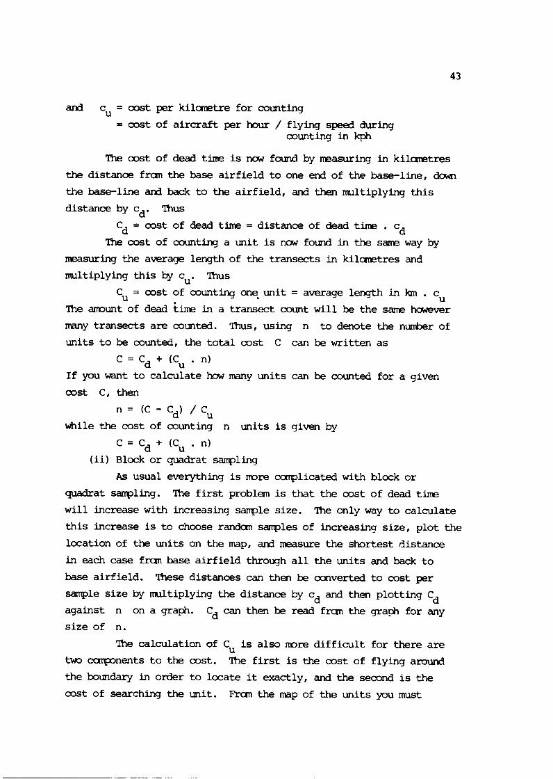
and cu = cost per kilometre for counting
= cost of aircraft per hour / flying speed during counting in kph
The cost of dead time is now found by measuring in kilometres
the distance from the base airfield to one end of the base-line, down
the base-line and back to the airfield, and then multiplying this
distance by cd. Thus
cd = cost of dead time = distance of dead tire . cd The cost of counting a unit is now found in the same way by
measuring the average length of the transects in kilanetres and
multiplying this by c . Thus
u = cost of counting one unit = average length in km . cu The amount of dead time in a transect count will be the same however
many transects are counted. Thus, using n to denote the number of
units to be counted, the total cost C can be written as
If you want to calculate how many units can be counted for a given
cost C, then
n = (C-
while the cost of
C = C +
(ii) Block or
As usual
quadrat sanpling .
Cd) / cu counting n units is given by
( C . n) quadrat sampl ing
everything is more carplicated with block or
Â¥Hi first problem is that the cost of dead time
will increase with increasing sairple size. The only way to calculate
this increase is to choose randan samples of increasina size, plot the
location of the units on the map, and measure the shortest distance
in each case fran base airfield through all the units and back to
base airfield. These distances can then be converted to cost per
sample size by multiplying the distance by cd and then plotting Cd
against n on a graph. Cd can then be read from the graph for any
size of n.
The calculation of C is also more difficult for there are
two components to the cost. The first is the cost of flying around
the boundary in order to locate it exactly, and the second is the
cost of searching the unit. From the map of the units you must

calculate the average boundary length in kilometres and the average
size of the units in square kilometres. The cost of flying the
boundary is found by multiplying the average length of the boundary
by c . The cost of counting is mre diff icul t . The best way is t o 2 calculate the ra te of ground coverage in km / hour from the speed of
the aircraf t during counting and the width of s t r i p that you think
you wil l be covering. From this calculate the time taken to count a
unit by dividing the average area of the unit by-the ra te of covering
the ground, and convert this Into cost by nultiplying it by the cost
per hour of the aircraf t . Add these two quantities together t o get an
estimate of the cost per unit.
The same fornula for total cost can be used,' only Cd must
new be read from your graph.
(iii) Other costs
These calculations wil l give estimates for the cost of
carrying out the census. In addition, one should allow for such
items a s the cost of personnel, the cost of putting out fuel dunps,
o r the cost of bringing in an a i rc ra f t from outside to do the census.
These costs can often be greater than those of the census i t s e l f .

SECTION 6 PRACTICAL ASPECTS OF AERIAL SAMPLE COUNTING
6.1 Introduction
Organising and carrying out a sample count requires a camon- sense approach to a large number of rather small practical problems.
Experience is necessary before things can be expected to go without
a hitch. It must always be borne in mind that an entire census can
be invalidated, and a great deal of time and money wasted, by
inadequate attention to small practical details.
The mininum crew comprises a pilot and an observer. The pilot
should never be called upon to count animals or to record data : he
has enough to do navigating, avoiding vultures, and maintaining
strict height, speed and bank control. Ihe time he spends piloting
will be at the expense of the time he can spend observing, and so his
observing will be inefficient. If he spends too much time observing
then his piloting will beccne unsafe. Pilots who claim they can do
both jobs are fooling themselves as well as everyone else, and census
results obtained by a pilot/observer should always be treated with
great scepticism.
It is our general experience that censuses go much better if the
pilot is also a biologist involved in the census. Ttlis ensures that
he has a real interest in flying correctly and in concentrating on
navigation, height and speed control. Non-biologist pilots sometimes
make poor census pilots as they tend not to appreciate the errors and
biases that occur through inaccurate piloting.
Pilots require much practice before they caul be expected to
carry out a census properly. Census work requires the ability to
navigate at lew level by reference to small ground features, a skill
that can only be developed through practice. Practice at speed and
height control is also required, especially the ability to react
swiftly to changes in ground level. A thorough familiarity with the
census area is also imprtant if consistent results are to be
obtained. Low level flying also requires experience in judging and
allowing for wind drift, and for the effect of winds around hills.
Census pilots should take every opportunity to practice these skills.
Similarly it takes much time and experience before an observer
becomes ski l led a t spotting and counting animals, therefore observers
should take every opportunity to f l y in order to become accustomed t o
this. Observers can be trained to count accurately by shewing them
colour s l ides of d i f ferent sized groups of animals. The photographs,
taken iron the nonnal height and viewing angle, are shown t o the
observer who is given ten seconds to count the nunber of animals on
each photograph. He is then to ld the correct number, before the next
s l i d e is shown. This r e su l t s in an extraordinary increase i n counting 4 9 accuracy . It mast always be rementoered that even highly experienced
observers consistently undercount the numbers of animals i n a group
by as much a s 40%. Observers a l so need mu& pract ice a t recording
data (either writing down o r tape recording) and in using a camera
and changing films. The more practiced the observer is a t doing this,
the more time he can spend observing. * The census organiser should not underestimate the u t t e r
confusion which can resu l t from incomplete understanding between
dif ferent members of the census team. A thorough briefing cf p i l o t
and observers is necessary covering the principles of the census, the
d e t a i l s of the flying, and the methods of counting and recording the
data. It is not enough, fo r ecample, just to tell an observer t o
count a l l the animals seen between the streamers. Exact instruct ions
must be given a s t o what t o do when a streamer cuts through a herd of
animals, o r when the same group of animals is seen t w i c e in supposedly
d i f ferent s t r i p s , o r when animals run in to o r out of the s t r i p a s the
a i r c r a f t passes by. Exact instructions must be given a s t o how t o
record the data, how to operate the tape recorder, how to use the
camera and what to do w i t h used films.
It follows from this that consistent r e su l t s w i l l be obtained
i f a crew of p i l o t and observer (s) can always work together a s a team,
fo r they w i l l then get used t o each o ther ' s work methods. Nonetheless,
it is quite amazing hew many s i l l y mistakes a re made even by
experienced crews. In one recent census am observer turned h i s tape
recorder ' o f f when he made an observation, and turned it 'on' when
he had finished. In another census an observer held the microphone
too close t o an open window so that only wind noise was recorded.
* See Appendix 2.

An observer once l o s t h i s spectacles out of the window (they should
be t i e d down with s t r ing) while another one mixed up t h e colurms on
h i s data sheet so that the elephant and eland observations were
randomly recorded i n tw colums both labelled 'el'. Aqain, one very
experienced observer forget to tape the lens of h i s camera a t in f in i ty
and a l l h i s photographs came out blurred.
6.2 Choice of Aircraft
As the observer mst have an unobstructed downwards view of the
ground only a i r c r a f t with high wings are sui table f o r census work.
Wing s t r u t s are a l so necessary i f t ransect sanpling is t o be employed,
fo r the streamers are attached t o these s t r u t s . Apart f r m this
there is no rea l constraint on the choice of a i r c ra f t . It should not
be too f a s t fo r otherwise the observer w i l l not have enough time t o
scan the s t r i p effect ively, nor should it be too slow otherwise it
w i l l t ake too long t o cover a census zone. Speeds ranqinq from
80 - 120 nph have been found sui table f o r ae r i a l census work, while
speeds fas te r than this should be avoided. It is a l so advantageous
i f t h e windows can be opened or removed altogether, f o r this great ly
increases the observer's counting accuracy. Wind can be deflected by
f i t t i n g small baf f les t o the window edges. A four sea ter a i r c r a f t is
a lso of advantage because two observers can be carried. This
inroediately doubles the area that can be searched per uni t time. The
fourth crew marter can always act a s a recorder, or help i n navigation,
o r col lec t other types of information.
The a i r c r a f t most commonly used f o r ae r i a l census work are the
high wing Cessna models 180, 182 and 185, and the high winq Piper
models PA-12 (Cruiser) and PA-18 (Super Cub).
6.3 Transect Sampling - General Flight Planning
(i) Safety
Aerial census work requires the a i r c r a f t t o operate over
inhospitable and inaccessible country, often qui te f a r from base, in
that part of the a i r space usually reserved f o r vultures. Safety
measures should therefore be taken seriously. Obviously the ai rcraf t
mast carry adequate f i r s t a id equipment, food and especially water,
and seme form of ground-air oonirunication equipment (flares,
signalling mirrors, radio). Further precautions should also be
taken. A map of the aircraft 's planned flight should always be l e f t
a t the hone base, and th is nap should also have expected ETAS a t
different points written on it. If two aircraft are carrying out a
census then they sbu ld be i n radio contact (listening out) the whole
tine, and they should report 'operations normal' a t fixed tines.
Each aircraft should also have a map showing the other a ircraf t ' s
planned flight. If an aircraft is landing for fuel a t another
airfield apart fran the base airfield, then it should report back its
arrival i f radio ccrrni-uiication is available. Similarly, that airfield,
i f manned (e .g . a guard post airfield) , should be told when t o expect
the aircraft , arid when t o report its non arrival. A back-up aircraft
for search and rescue should always be available as we l l , of course,
as suitable ground vehicles.
(ii) Fuel management
It is the pi lot ' s responsibility to ensure he has enough
fuel to carry out a census fl ight, ensuring that he always has a
safety margin to allow him to reach an airstrip. Fuel often has t o
be located on outlying airfields so that the aircraft can refuel
without having to return to base. In this case some method of getting
the fuel into the aircraft is required, which is sometimes forgotten.
A punp and f i l t e r are necessary, as wel l as some method of opening
the drums ( this is frequently forgotten) . If o i l is supplied, then
seme form of oil-can is also necessary.
(iii) Planning the flights
Â¥Hi mst usual arranqement for an aerial transact count is
for the transacts t o be flown in order, starting a t one end of the
census zone and working through t o the other. This arrangement works
well for snail census zones that can be covered in a single flight of
2 - 3 hours, but the flights have t o be broken up in sane way i f the
census zone is larger than this. Care must be taken here, especially
i f the animals move systematically within the area. For exanple, i f
the water is a t one end and the grazing a t the other, serious errors
could result f m censusing one end in the rooming and the other in
the afternoon. If more than one flight has to be made to cover a

census zone then the best plan is to d i s t r i b u t e the f ly ing over the
whole area on each f l i g h t . For instance, i f 24 t ransac ts are t o be
flown in two f l i g h t s , choose twelve a t random f o r the f i r s t f l i q h t ,
and do the second twelve in the second f l i q h t . This w i l l in no way
increase the costs of t he census.
( i v ) More than one a i r c r a f t
I f two, o r more, a i r c r a f t a r e carrying out a census then
things cfet a b i t more carpl icated, f o r each crew w i l l inevitably have
s l i g h t l y d i f f e r en t biases and e r r o r s i n the way they carry out the
census. I f there are two d i s t i n c t census zones, o r perhaps s t r a t a ,
then one a i r c r a f t can be assigned t o each. Alternatively, in the case
of a s ing le large census zone, one a i r c r a f t can be assigned t o one
part and the other t o the remainder. This is in e f f e c t the same a s
dividing the census zone i n t o two separate parts, the r e s u l t s
subsequently being worked up separately fo r each zone. Final ly , i f
the census organiser is very sure of t h e competence of both p i l o t s ,
then one a i r c r a f t can have assigned to it half of the t ransec ts ,
chosen a t random, the rest being assigned to the other a i r c r a f t .
This entails sane safe ty problems fo r the a i r c r a f t may frequently be
operating close to each other . Under these conditions the
observations from each a i r c r a f t would be pooled in the analysis of
the f i n a l r e su l t s . In general, however, it is best t o keep the
a i r c r a f t well apar t i f possible. I f they nust operate in the same
area then it is w i s e to have them working in the same direct ion. For
example, it is askinq f o r t rouble i f one a i r c r a f t works from west t o
e a s t and the other from e a s t t o west. Final ly , when two o r more
a i r c r a f t are working together it is absolutely essen t ia l t h a t a l l
p i l o t s know exact ly where the other a i r c r a f t w i l l be.
(v) Other fac tors
Observers should never be required to count f o r more than
three hours a t a s t r e t c h otherwise they become tired and their
counting e f f ic iency f a l l s o f f . In very lonq censuses, no crew,
however tough they might consider themselves to be, should work f o r
more than tw days w i t h o u t a morning's or afternoon's break.
Counting should a l s o never be attempted during t h e heat of the day
because animals lie up in shade and are impossible to see, nor

should it be attempted when the light is highly directional (e.g.
early in the morning and late in the afternoon). In East Africa the
best hours for counting are between 8 a.m. and 11 a.m., and between
3 p.m. and 5 p.m. local time. These constraints nust be considered
when planning the flying.
6.4 Transect Sampling - Piloting ( i) Navigation
Flying a transect count requires following, with a high
degree of accuracy, lines marked on a map of the census zone. The
only practicable method of navigation is by reference to ground
features, which means that an accurate large scale map is essential.
It is possible to use a 1 : 250,000 map if it is very detailed but
in general a 1 : 100,000 or even a 1 : 50,000 map is better,
especially when censusing a small area. If the transects are very
long then sane oancpranise trust be reached between large scale and a
map of manageable size. If no maps are available then vertical
aerial photographs can be used, or even photo-mosaics, for these show
up most of the drainage lines, small hills and vegetation boundaries
that are most useful for navigation. Maps can always be annotated
with tracks etc. to make subsequent censuses easier to carry out.
The transects are marked on the map as a single line down
which the pilot should attenpt to fly straight. Wind drift can be
assessed on the first few transects and the appropriate ampass
headings selected. It is a mistake, however, to rely too heavily on
the compass and reference to ground features must always be the
primary navigation aid.
In seme types of systematic transect counts, or when
distribution data are required, each transect has to be subdivided
into units at regular intervals along its length, the pilot
informing the observer(s1 as the aircraft passes from one unit to the
next. Although in most cases these subdivisions can be located by
ground features, inevitably there will be sane featureless areas
where they have to be located by time. The pilot should carry a
stop watch in this type of survey and should zero it and restart it
at each boundary throughout the flight. When flying over really

featureless country it is a good idea fo r the p i l o t t o have written
down in advance the time expected to be taken f o r each transect. A
check on elapsed time can prevent r ea l ly wild er rors in navigation.
It is of course the p i l o t ' s responsibili ty t o tell the
observer (s) when t o start counting and when to stop a t the end of a
transect.
It is inevitable that occasional wild errors i n navigation
w i l l occur, usually taking the form of ending a transact some
kilometres from where you should be. The p i l o t can do one of tvro
things. F i rs t ly , he can f l y the t ransect again, in which case the
data collected on the f i r s t attempt a r e ignored. Alternatively, he
can mark on h i s r a p the point where he f ina l ly finished up, and then
go on t o the next transect. In this case the error can be corrected
f o r when working up the resul t s . It a l so somettmes happens t h a t
large storms prevent a number of t ransects from being flown along in their ent irety. All the p i l o t has t o do here is to mark on h i s map
where t h e t ransects a re broken off and where the next ones are
star ted. These errors can a l so be corrected fo r l a t e r .
(ii) Height control
This is one of t h e most important aspects of t ransect
pi lot ing fo r the width of the t ransect s t r i p as demarcated by the
streamers is d i rec t ly p r o y r t i o n a l t o the a i r c r a f t ' s height above
the ground. The higher the a i r c r a f t t h e wider w i l l be the s t r i p , and
v ice versa. Serious biases can thus creep in unless the p i l o t pays
very careful at tent ion to height control. For exanple, i f the p i lo t
always f l i e s too high then the s t r i p w i l l be wider than t h a t
calculated, and the sample estimate w i l l be biased i n an upwards
direct ion leading t o an overestimate of numbers.
The only rea l ly sat isfactory way t o achieve height control
is t o have a radar alt imeter f i t t e d in the a i rc ra f t . This instrument
gives continuous readings of the actual height above the ground,
enabling the p i l o t to f l y more accurately. The rea l advantage,
however, is t h a t the readings from the instrument can be written
down (by someone other than the p i lo t ) a t regular intervals (e.9.
once every minute) so tha t a f t e r the census the actual height flown
can be calculated. This actual height can then be used t o calculate
the actual width of the s t r i p during the census. It is our
experience t h a t p i l o t s can m a i n t a i n very accurate and very precise
height control when using a radar alt imeter 17,38
A radar alt imeter, l ike any other instrument, is prone t o
error and it is essent ial to ca l ibra te the instrument against the
pressure altimeter a t the s t a r t of each f l i g h t in a census. The
cal ibrat ion is carr ied out a s follows. The a i r c r a f t is flown a few
f e e t above the ground a t f u l l cruising speed while the pressure
altimeter is set t o a convenient reading ( a ce i t a in steadiness of
hand is required to do t h i s ) . The a i r c r a f t then f l i e s to the
desired height a s shown on the pressure altimeter and maintains this
height fo r a few minutes t o allow the pressure altimeter t o settle
down and to allow the radar alt imeter t o warm up. A number of passes
are then made over the point where the pressure altimeter was set,
and the readings from both al t imeters are recorded. The radar
alt imeter can then be calibrated against the pressure al t imeter ,
and any error corrected for.
An al ternat ive method is to use the ' shadow m e t e r ' which
is a device whereby the a i r c r a f t ' s height above the ground can be
judged by matching the s i z e of its shaded on the ground against marks
on the wing s t r u t . I f the wings a re level then the s i z e of the
shadow on the ground is constant, and equal to the wing span. The
method of constructing a shadow meter f o r a d e s i r d height is shown
in Fig. 9. I t is a remarkably ef fec t ive device. Once it is set up
then it must be calibrated against the pressure altimeter in the way
described above. After se t t ing the pressure altimeter when close t o
the ground, the p i l o t passes a number of times over the same point
adjusting h i s height by the shadow meter and taking readings from the
pressure altimeter.
When using a shadow meter during a transect count it is w i s e
to wri te the pressure altimeter readings on the map a t odd points
along each transect. These can then be used on successive t ransects
should the sun be temporarily hidden. It is essent ia l t o do this in
four sea ter a i r c r a f t f o r the p i l o t wi l l only be able t o use the shadow
meter on every other transect. The shadow meter works best a t low
a l t i tudes being ef fec t ive a t flying heights of up t o about 4 0 0 f t

Fig. 9 Constructing the Shadowmeter
diagram after Pennycuick 1973 4 2
prop the a i r c r a f t i n the f ly ing posi t ion and measure the
height of the p i l o t ' s eye above the f l o o r (h )
i f H is the required f ly ing height
B is the wing span of the a i r c r a f t
ca lcu la te b = B . h / H
mark on the hanger f l o o r in te rva ls of width b
mark a l t e rna t e black and white marks of t he strut as shewn.

(120 metres) above the ground.
mansect counts can be carried out with no other aid than
the pressure altimeter provided that the ground is nearly horizontal,
as for instance when the census zone is a flood plain3 o r an old
lake bed. I f certain parts of the area are raised then the p i lo t , should know their elevations in advance so that he can adjust h i s
height when flying over them. The pressure altimeter mst f i r s t be zeroed at the start of
the f l ight by making a low pass over the ground. A progressive
altimeter error will develop during the day as a result of change in
the ambient barometric pressure, so it is essential to re-set the
altimeter every half hour o r so. For this purpose a nurtoer of f l a t
open places should be selected in advance where ground height a t
each, relat ive to the original reference point, mst be h a m . When
a check is due, the p i lo t breaks off a t the end of a transect, f l i e s
down to ground level over one of these check points, sets the
altimeter and informs the observer of any error. Ttie actual height
flown, and therefore the actual s t r i p width, can then be calculated
for each half hour period.
(iii) Aircraft bank
The overall effect of a i rc ra f t banking is t o make the s t r i p 4 1 width, as seen by the observer, larger than calculated . The reason
for t h i s is that, for an observer viewing from one side of the aircraf t ,
the errors of inward and outward bank do not cancel each other out.
Inward bank reduces the s t r i p width, but an outward bank of the same
order increases the s t r i p width t o a much greater extent in
caparison with the reduction of s t r i p width caused by inward bank.
Therefore, banking w i l l cause a positive bias to the resul ts of the
census. The p i lo t nust therefore try t o maintain the wings in as
near a horizontal position as possible.
6.5 Transect Sampling - Observing
(i) Defining the counting s t r i p
In a transact count the boundaries of the s t r i p within which
the observer h a to count the animals are defined by streamers
attached to the struts of the aircraft . The streamers f l y out behind

the struts in the airstream, being seen by the observer as tracing
two parallel lines on the ground. Having decided upon the required
flying height and s t r i p width, the position of the streamers are set 4 1 u p a s follows :-
(a) pmp the aircraft in the flying a t t i t& on a level surface,
trestling the t a i l in the case of a tail heel aircraft. Have the
observer sit in h i s place making sure he is ocmfortable and that he
is looking out of the window in a relaxed position. (It is of
considerable help i f the observer has already made a t r i p in the
aircraft beforehand so that he knows a comfortable position to sit
in. ) Measure the height (h) of the observer ' s eye above the floor
(Fig. 10) . (b) choose the position of the inner streamer ( a i n Fig. 10) on
the strut so that the observer's line of sight through it is clear
of the wheel but still as close t o the body of the aircraft as
possible. Place a marker A on the ground on this line of sight, and
get the observer to make a mark a ' on the window so that his line of
sight passes from a ' through a t o A.
(c) place a second market on the ground a t B. The distance from
A to B is denoted by w, and it is found from the formula
w = W.h/ti
where W is the required s t r ip width and H is the required flying
height. The two heights h and H must be expressed in the sama
units, as also nust w and W.
(d) place the second streamer a t b on the wing strut in the
observer's line of sight to point B. The observer must meanwhile
keep his l ine of sight through a ' - a - A, while making a second mark
on the window a t b' t o establish a second line of sight b' - b - 5. When a l l these marks are correctly positioned the observer's two
sight lines should be in line when he sits in his comfortable
position.
pe marks a ' and b' on the window ensure that the
observer's head w i l l always be in the correct position during flight.
These marks must be kept lined up w i t h the marks a and b on the
struts, for the s t r ip w i l l appear wider i f the observer slumps in his
seat, and narrower i f he sits upright. If the windows are taken out
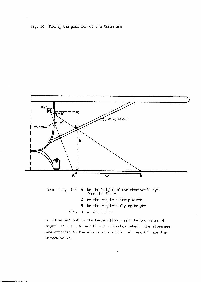
Fig. 10 Fixing the position of the Streamers
from t e x t , l e t h be the height of the observer's eye from the floor
W be the required s t r i p width
H be the required flying height
then w = W . h / H
w is marked out on the hanger floor, and the two l ines of
s ight a ' - a - A and b' - b - B established. The streamers
are attached t o the struts a t a and b. a ' and b' are the
window marks.


during f l igh t then sane alternative method of marking nust be used,
e.g. marks on the window frames.
The width of the s t r i p is also altered by any bank of the
aircraft. Both these errors are minimised i f the s t r i p is as close
to the a i rc ra f t as possible, without the wheel being in the way and
without the observer having to lean out of the window.
Heavy builder's s t r ing is ideal for the streamers. The
str ing mist be securely taped to the strut so that it can not s l i p up
o r down. The length of the str ing w i l l be determined by the
characteristics of the airflow around the particular a i rc ra f t , but in
general the streamers should be as long as possible. W i t h seme a i rc ra f t it is possible to attach small p las t ic funnels to the end of
the streamers. This makes them f l y more evenly in the slipstream.
Some a i rc ra f t have such turbulent airflow around them that thin
wooden rods have to be used instead of string. They can be attached
to the struts w i t h ' jubilee' c l ips , being positioned in exactly the
same way.
The s t r i p width set up in this-way w i l l be approximately
correct. A calibration f l igh t must however be carried out t o make
sure that it is reasonably close to the required width. A line of
markers nust f i r s t be carefully la id out. White blocks, o r pieces of
cardboard, measuring sane 100 x 40 am are suitable. They should be
placed twenty metres apart on a suitably f l a t piece of ground. The
line of markers should be a t least twice the intended s t r i p width,
and every f i f t h market should be double o r treble i n width.
A t the start of the calibration f l ight the pi lot makes a low
pass over the markers and sets h i s pressure altimeter before climbing
up to the required flying height. H e should then make a t least twenty
passes a t r ight angles across the line, recording h i s height a t each
pass. The observer meanwhile counts, o r photographs, the number of
markers between the streamers. The width of the s t r i p is directly
proportional to the height of the a i rc ra f t , which is found as follows :-
l e t h be the average height of the a i rc ra f t during, say,
20 passes
w be the average s t r i p width during those 2 0 passes
H be the selected flying height during the census

and W be the nominal s t r i p width a t that flying height
then, W = w . H / h
If this nominal s t r ip width W is widely in error then the streamers
can be repositioned and another calibration fl ight made.
(11) Counting The observer most continually scan the s t r i p defined by the
streamers, spot groups of animals, decide whether or not they are inside the str ip , count them and record the data. The observer can
move his head around when spotting for groups of animals but he nust
always return it to the correct position (1.e. he must line up the
window and strut markers) to decide i f the animals are i n the s t r i p
or not. Single a n M s , or -11 group , can be mtd bdlvidually,
but with larger groups the observer may have to count in 'fives' o r
tens1. It is here that previous training given to the observers is
valuable. Animals seen w i t h i n the s t r i p are counted, and those
outside the s t r i p are not. If a streamer cuts through a herd so that
sane animals are in and sane are out, only those inside the s t r i p are
counted.
There are four very cannon mistakes made by observers on
transect counts :
(a) i f the aircraft is too low they count animals just outside the
strip. (b) i f the aircraft is too high they ignore animals that are just
inside the strip.
(c) i f they see the same group of animals twice in two different
stripe, say because the animals have moved, they ignore them on the second occasion.
(d) i f the pilot makes an error i n navigation, for example when
neighbouring s t r ips are close together, and the observers
notice this, they do not count the animals seen in the strip.
These are very bad mistakes to make. In (a) and (b) the observer is
trying to conpensate for errors in height control, but these errors can be taken care of a t a la te r stage when the results of the census
are worked up. In (c) the observers f a l l to realise that those
animals unmfed twice w i l l on average be ampmated for by those
missed altogether, so long as the animals axe moving independently

of the aircraft. Similarly, i n (d) the areas counted twice are
obviously balanced by those areas missed. Another mistake made by
observers is to compensate for any bank of the aircraft, and they
tend to count a sl ightly w i d e r s t r i p when the wing is down and a
narrower s t r i p when the wing is up. None of these things must be
dcxie, for the excellent reason that errors caused by height control,
bank control and navigation can be capensated for a t a later stage,
but only so long as the observers have always counted everything that
they see within the streamers.
The rule that observers mast follow absolutely is that
i f an animal is within the streamers then it nust be counted, and i f
it is outside the streamers then it is ignored.
(iii) Recording data
Datanay be recordedeither by tape recorder o r b y w r i t i n g
down, the form& always being preferable because the observer does
not have t o take his eye off the s t r ip . The small cassette tape
recorders are best for t h i s purpose because of their oonpact size.
Any model with manual control of recording level (so that it can be
adjusted to the engine noise) incorporating an an/off switch on the
microphone is ideal. A good supply of spare tapes and batteries mist
of course be carried. The recorded should be checked before take off ,
Imnediately a f t e r take off , and at the end of each transect . The recorder need only be switched on when an observation is to be
recorded, bat it is important too remember to allow the tape to get to
full speed before speaking. When tape recording, the observer should f i r s t record the
tAce off tim and t b dab, andmst identify each transect by nunber,
noting the start and finish time of each transect. Animal numbers
must be recorded In sane oanpletely unambiguous form. It is usually
best too give the species f i r s t , followed by the nuirber in each group;
e.g. "zebra 21; elephant 3;" etc. I f anything has to be repeated o r
corrected, say "correction" or "say again" before repeating the item. In this way it is quite clear during transcription that the same item
has been recorded twice, and is not two separate items.
Transitions between vegetation types can be recorded, and
miscellaneous observations on f i r e , greenness of grass, water,
sub-divisions of transects etc. can be interjected a t any time.
I f writing down has t o be used then an adequate supply of
ruled recording sheets, as well as pencils etc. , mist be made ready
beforehand. There mist be a separate mlunn for each species, each
colunn clearly labelled, w i t h a spare oolunn on the l e f t for the
transact number, the start and finishing tiroes etc. Transitions
between vegetation types of sub-divisions of the transects, can be
marked in by drawing a l ine across the data sheet, but i f too much
is attempted the observer spends more time writing than observing.
The numbers of animals written in the appropriate colurm,
must also be unambiguous. Thus, i f three zebra are seen, then two, then six, write them down as 3 / 2 / 6 /; otherwise it may be
Impossible afterwards t o be sure whether you say a three and a twenty-six, a thirty-- and a six, o r even a 326. A t the end of
each transect a horizontal line should be drawn across the data
sheet and the next transect number entered below it.
W r i t i n g down is on the whole a too time consuming method
for a nulti-species count, especially i f the density of animals is
high o r i f the habitat makes them at a l l d i f f icu l t to see. Writing
down is also a potent cause of airsickness. In four sealer a i rc ra f t
the fourth crew member s i t t i ng alongside the pi lo t can ac t as a
recorder and write down the observations which the observers call out. In noisy a i rc ra f t an intercom system should be f i t t ed , but it nust be
remembered that a t times things can become very hectic w i t h both
observers shouting out excitedly. Errors are bound to creep in.
Another very useful task for the recorder is to write down
the readings from the radar altimeter.
( iv) Photographing large herds Experience shews that even experienced observers are unable
to count herds of animals nuntering more than about twenty individuals
w i t h any degree of accuracy. They consistently undercount, somBtlmBS 3,49 by very large margins Large groups ahodd always be photographed,
the nunter of animaps being counted l a t e r from the photographs. A
visual estimate of the photographed herds must a lso be made in the
case of photographic fai lure, o r in case the film is lost o r
destroyed in the developing process. The census organiser must

impress upon the observers the importance of getting good
photographs, and he must also tell them precisely the minimum group
size for photography. The safest method is to photograph any group
larger than five individuals, especially if elephant are being
counted. On a malti-species count this could well 'overload' the
observers, so a minimum size of ten animals should be used.
Any good 35 mn single-lens reflex camera is suitable. A
50 mn or 80 mn lens has been found adequate as it gives good
images of the animals while allowing the transect streamers to appear
in the photographs. Ideally a zoom lens would be used but these are
still very expensive. Colour film gives better results than black
and white unless conspicuously mnochrcme animals such as buffalo and
elephant are being counted. A reasonably fast film (e.g. 400 ASA) is
required as l/250th sec. is about the slowest shutter speed which can
safely be used. Some colour films can be over-rated to overcame poor
light (e.9. High Speed Ektachrome can be rated at 650 ASA with no
noticeable loss of quality) but they must then be specially developed.
The photographs mast be taken from the fixed head position,
e.g. with the window and strut markers lined up as seen through the
camera. This requires a lot of practice on the part of the observer.
Â¥Illi is, in face, only absolutely necessary if the streamers cut
through a portion of the herd, for if the herd is clearly seen to be
between the streamers then any convenient photographic angle can be
used. It is, incidentally, a good idea to put black marks along the
inner streamer so that the inner and outer streamers can be
distinguished on photographs.
Certain other precautions must be taken. The camera lens
should be taped at the infinity focus position. Each film should be
nunbred before the census starts, both on the cassette and on the
film leader. This nurrber on the leader must be scratched into the
enulsion (for otherwise it can vanish during developing) and it must
also be underlined (to distinguish later between - 6 and - 9 ) . The
observer must record each film number on his tape or data sheet when
he starts a new film, and used films mast be put well out of the way.
It is a good idea to rewind used film canpletely into the cassette
before unloading. There is then no chance of using the film again

by mistake.
A conpletely unairbiguous recording system nust be used so
that the sequence of photographs can be matched l a t e r to the v i sua l
estimates and to the d i f f e r e n t t ransec ts . Fig. 11 shows a system
that has been found to work well f o r both tape recording and f o r
wri t ing down. When tape recording it is v i t a l to record the data in
the following form : f i r s t the species, then t h e v i sua l estimate,
then the number of frames taken. For example, a tape record might be
'elephant, six, one frame; elephant, ten, three frames; bufffalo ,
twelve, one frame" etc. I f this were muddled up so that it was
recorded as "elephant, six, one frame, three frames, elephant, t en ,
buffalo, twelve, one frame ..I1 etc. it would be impossible t o decide
during t ranscr ip t ion i f the three frames re fe r red to the f i r s t or
second elephant observation. When writ ing down, a new line mst be
started a f t e r each photograph otherwise it w i l l be impossible t o
disentangle the sequence of photographs a f t e r the census.
Fig. 11 shows the commonest s i t ua t ions encountered.
(a) and (b) are the simplest s i t ua t ions when either a s ing le frame
or a number of overlapping frames are taken of the same group.
(c) there are a number of overlapping frames a s well a s a s ing le
frame of a sub-group of the main group. TTie estimate r e f e r s
to a l l t h e photographs together.
(d) there are a nunter of independent frames with no overlap, and
the estimate again r e f e r s to a l l the photographs.
(el here two independent frames have been taken of t he - same group.
The estimate therefore r e f e r s t o only one of the photographs,
no t to the total number of animals on both. Only one of the
photographs would then be used a s a count of t he group, i.e.
the better one.
This convention of x + y dis t inguishes between independent
photographs of the same group when the estimate r e f e r s to only one
of the sets of photographs. A large group may need many overlapping
f rams and the observer may lose count. In this case a blank frame
should be taken by exposing a frame w i t h t he camera held against a
knee. This blank must be recorded, e.g. "buffalo, four hundred,
many frames, one blank."

Fig. 11 System f o r recording frame numbers and estimates when using photography
Tape record Writing down
a) only one frame
b) two overlapping frames
c) two overlapping frames, and a sub-group
dl many independent frames
e l two independent photographs of the same group
Note : the c i r c l e around the number of frames i n the written record distinguishes t h i s from the number of animals recorded.

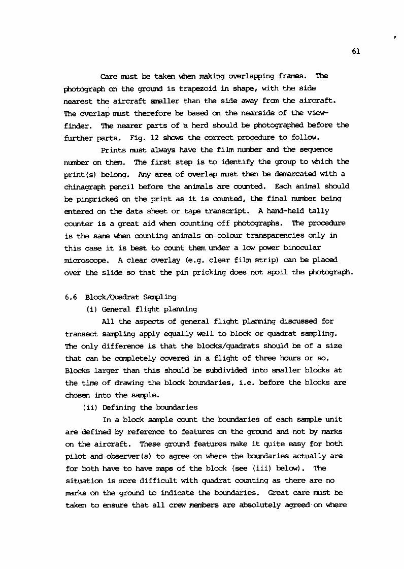
Care must be taken when making overlapping frames. The
photograph on the ground is trapezoid in shape, w i t h the side
nearest the a i rc ra f t smaller than the side away from the aircraft .
The overlap must therefore be based on the nearside of the view-
finder. The nearer parts of a herd should be photographed before the
further parts. Fig. 12 shows the correct procedure t o follow.
Prints mst always have the film number and the sequence
number on them. The f i r s t s tep is t o identify the group to which the
pr int (s) belong. Any area of overlap nust then be demarcated w i t h a
chinagraph pencil before the animals are counted. Each animal should
be pinpricked on the print as it is counted, the f inal number being
entered on the data sheet o r tape transcript. A hand-held t a l l y
counter is a great aid when counting off photographs. The procedure
is the same when counting animals on colour transparencies only in
this case it is best to count them under a low power binocular
microscope. A clear overlay (e.g. clear film s t r ip ) can be placed
over the s l ide so that the pin pricking does not spoil the photograph.
6.6 Block/Quadrat Sampling
(i) General f l ight planning
All the aspects of general f l ight planning discussed for
transect sampling apply equally well to block o r quadrat sampling.
f ie only difference is tha t the blocks/quadrats should be of a s ize
that can be oonpletely covered in a f l ight of three hours o r so.
Blocks larger than th i s should be subdivided into smaller blocks a t
the time of drawing the block boundaries, i.e. before the blocks are
chosen into the sanple.
(ii) Defining the boundaries
In a block q l e count the boundaries of each sample uni t
are defined by reference t o features on the ground and not by marks
on the aircraf t . These ground features make it quite easy for both
pi lo t and observer(s) t o agree on where the boundaries actually are
for both have t o have naps of the block (see (iii) below) . The situation is more d i f f icu l t with quadrat counting as there are no
narks on the ground to indicate the boundaries. Great care nust be
taken to ensure tha t a l l crew members are absolutely agreed-on where

the boundaries are. It is best to spend sane time f lying around the
boundaries u n t i l agreement is reached. Always play sa fe by f ixing on
s l igh t ly larger boundaries than those ca l led for. The location of
each group of animals has to be marked in on a map anyway (see below)
so afterwards a f i n a l decision can be made as t o which animals are in
and which out.
(iii) Flight patterns and counting
Ttte choise of procedure is more f l ex ib le than in transect
counting because the exact f l i g h t path is not l a i d down in advance,
and it is up to the crew to decide exactly where, and a t what height
to f l y . The observer is now required t o find and count every animal
in the block, and t o avoid counting any twice, a problem that does
not arise in transect sanpling.
A s p i r a l f l i g h t pattern is su i tab le f o r small blocks where
the l i g h t is not highly direct ional . The p i l o t f l i e s around the
boundary of the block and then s p i r a l s in towards the middle, w i t h t h e
observer looking inwards towards the centre of the block throughout.
The zig-zag pattern is best f o r large blocks and in
s i tua t ions where the sun is low in the sky, f o r the f l i g h t pat tern
can be arranged so that the observer always looks down sun throughout
the count, changing s ides on each beat. The f i r s t beat should always
be flown jus t outside the boundary so t h a t the observer can see t h e
actual boundary a s he looks in to the f i r s t s t r i p .
In block counting the basic f l i g h t pat tern is only a
skeleton on which the d e t a i l s of t h e f l i g h t are based. In h i l l y
country a cannon variant is to nodify the basic zig-zag pat tern by
following ridges and valleys. In the case of a large block t h a t is
divided by a prominent ridge o r r ive r it may be best to treat it as
two sub-blocks.
The most d i f f i c u l t part of block counting is t o ensure that
the entire block has been searched but t h a t no animals have been
counted more than once, and this becomes qu i t e hard to do w i t h large
blocks that may contain many animals. This is basical ly the
observer's responsibi l i ty , it being up to him to keep t rack of the
area which has been covered and to tell the p i l o t t o deviate a s
necessary to f i l l i n any gaps. The observer must keep track of the

Fig. 1 2 To ensure overlap on photographs, the nearside of the
viewfinder must be used.
a) no overlap on the near side misses some animals
AIRCRAFT
b) correct overlap; all animals are photographed
AIRCRAFT


aircraft's position by marking in the flight line on his map as well
as the area scanned (Fig. 13). He must also ensure that there is
some overlap between one strip and the next. Each group of animals
mast be given a serial ninter which is then marked in on the map in
the position where the group was seen. The species and number of
individuals is recorded on a separate data sheet or tape, along with the frame nunteers of any photographs taken. In this way the map
serves as an up-to-date record of the animals seen without becoming unduly cluttered. This procedure keeps the risk of double counting within reasonable bounds, and gaps in coverage become evident while there is still time to rectify them. The observer nust also record the start and finish time of each block.
The flying height is variable and will depend upon the
species being counted and the thickness of the vegetation. The great
difference between block and transect sampling is that in block
counting the important thing is to be able to spot groups of animals.
The aircraft can then deviate to the group in order to count it. A
height of 500 - 700 feet is very suitable for elephant and buffalo in
reasonably open country, while a much lower height would be required
for impala or gazelle. The distance between successive beats will
also depend upon the species concerned as well as the thickness of
the vegetation. With elephant and buffalo in fairly open country a
distance of 1.5 to 2 tan is possible4g, whereas with smaller species
a very much narrower strip would be necessary (e.g. 300 - 400 metres). The strip width for a block count can only be discovered by trial and
error in the area concerned. The most important thing, however, is
that there must be sane degree of overlap between successive strips.
Large groups of animals should always be photographed for
m t i n g later, k t a visual estimate should also be made at the same
time. For compact herds of animals a single oblique photograph will
suffice. For larger herds, especially buffalo, the pilot nust make a
straight-line pass alonq the herd so that the observer can take
overlapping photographs. The pilot must not circle the herd
otherwise it becomes out of the question for the observer to ensure
that he has photographed all the animals, and it becomes totally
lirpossible to sort out the areas of overlap on the photographs (Fig.14).

Block anmts becuw diff icul t to carry out i f many
species are being mmted - unless the dmsity of each is low. They are thus best suited t o single species c a n t s f and ta highly
conspicuous species a t that.
6.7 An ' Ideal' Aircraft/Crew
EVeqaw has slightly d i f f e r a t ideas of the best aircraft/crew
configuration for aerial w l e counting. An ideal arrangemntf i f
mney were no object would be the follwing.
Aixcraft : a Cessna 182 (or 180) high-wing mnoplane f i t ted with
long range fuel tanks and a radar a1timte.r. The rear windows wuld be made rmvable , and the rear bench mt
wuld be replaced with tvm separate chair seatst each
inclined slightly outbard.
Crew : pilot : concerned with navigatbnf height and speed
m t r o l etc.
recorder : si t t ing alongside the pi lot t helping with
navigation t W e p i n g recording radar a l t m e r
readings, recording other information (e.g. range
&itionsf etc.)
2 observers : in the rear seatsf equipped with mtorised
Nihn a m r a s with 5-0 - 80 m zoun lenses and 250 -sure
casettes. They would also have tape recorders with
throat micmghmes and earplug playbackf with the recorder
controls attached to the m a s .
Fig. 1 3 An example of a block count using the zig-zag f l i g h t l ine.
the observer has marked in t he a i r c r a f t ' s path (except f o r
odd diversions) and h a shaded t h e searched areas. As each
p u p is seen it is given a number, plot ted on the mp, and
entered on the da ta sheet.
m l e of Data sheet
BLQCK 7 N c : 5 Y k5N Observer : A. 8 c , D. E . F. Date 15. 4.72 Pi lo t : )(. y, z, S t a r t : egt5
Finish : f020
-up Species E s t h t e F r m s F i h No. Photo count
Note : 6 = buffalo, E = elephant

Fig. 1 4 When photographing a large hen3 the .p i lo t must make a
straight line pass along it. He nust not circle.

7.1 Int-ction
Like everything else to do with aerial sanple cuunting, working
up the results is 90% m n - s e n s e and 10?1 rule following. me me- discussed belaw are based on those of and the sam
terminology is used.
It seam sensible t o discuss the mthcds in term of a mrked
-1e fran a fairly straightforward type of aerial sample count. 2 The data cane frun an aerial transect camt of a 2829 Ian census zone
(Mch is here referred to as the 'northern study area') . A base-
line of 69 km was constructed, along which twelve randm points were
&sen. The transects were run thrmqh these p i n t s a t right angles
to the base-line, cmssing the census zone f m one side to the other.
l%e tramects varied i n lmqth be- 15 and 47 km. A far-seater
aircraft w a s used, w i t h the pilot taking care of navigation and
height mtml, the recorder d i n g records of the reading f m the
radar al t imter once every minute, and two obsemers in the back who
were using tape recorders and m a s . The animals amnted were
w i l d e b e e s t , giraffe, topi and inpala. Any group larger than ten
animals w a s * t o g r a m as well as estimated visually. The
observations were sp l i t up into successive 5 km intervals along each
transect so that distrikution data could be obtained, the pilot
calling out to the observers when each sub-unit was started. The
ncuninal flying height for the census was three hundred feet.
Calibration flights before the census SM that this gave a nunha1
s t r ip width of 514 metres; 244 mtres for the l e f t hand observer,
and 270 mtres for the right hand observer.
The f i r s t pint to consider is that the transects rn of
different length, for this w i l l obviously inflate the q l e variance
because the longer transects w i l l tend to have mre animals h than
than the shorter ones. This is takm care of in the analysis by
us* J O U ~ ~ S ~ t t x x ~ 227 for m-1 sized sampling units. 1n this
method the area of each of the transects has to be knam, as w e l l as
the area of the whole census zone. The second p i n t is that t m
observers were used. Unfortunately, it is not possible to treat

each obeemer's observations as thcxqh they vere -t, so the
observations have to be mrged once can t ing bias is c o w for.
mis s&ly mans that I& n-s of m s counted by
&servers along the length of each transect are ad%d tqether.
Similarly, the s t r i p width is taken t o be the sum of both observers'
strip.
7.2 The Stqes in the Analysis
Them are b a s i a l l y six stages to g3 through :-
calculating the actual s t r i p w i d t h , a N (m total
mmbr of units in the poplat ion f ran which the twelve
transects -re chosen)
calculating the area of each t r anse~t , a x l the area of
the census zcne
transcribing each obsemer's observations mto r m data sheets, and anmting the photographs
mrrecting each chemx's camtlng bias frun the
*-am m r g h g the observations fran each obeemer, and checking
for consistency
preparing the f inal data sheets, and calculating the
p p l a t i o n estimates.
Note that the data franeach 0-r are kept 'separate' unt i l the
last stage.
(i) Calculating the actual s t r i p wldth, and N
The nanhal s t r i p width for this census was 514 mtres at a
mninal flying height of 300 feet. This was fomd in t b way
described in Section 6.5 (i) (page 53) . The actual s t r i p w i d t h
during the census w i l l of cuurse depend upm the actual fly- height,
a d this is found by averaging a l l t h recordhgs fran the radar
a1tbete.r. In t h i s -1e the actual flying height was found to be
320 feet. The actual s t r i p width is now fomd by using the sane
f o m l a for calcula tbg the naninal s t r i p width.
let h be the nanhal flying height (e.g. 300 feet)
w be the nanba l s t r i p width (e.g. 514 e n s )
H be the actual flylng height (e.g. 320 feet)

W be the actual strip width
then, W = w . H / h = 514 x 320 / 300 = 548 metres = 0.548 km.
Thus, at the actual average flying height of 320 feet during
the census the actual average strip width was 548 metres.
N is the total nunter of units in the population from which
the sample was drawn, which in an aerial transect sample count is
found by dividing the length of the base-line by the actual strip
width during the census. In this exanple the base-line, measured
from the nap, was found to be 69 km in length. N is therefore
given by N = 69 / 0.548 = 126
Thus, 12 out of a possible 126 transects were sampled,
giving a sample fraction of 12 / 126 x 100 = 9.5%.
It will be realised that most of the bias from inaccurate
height control is removed by using the actual strip width in these
calculations.
(ii) Calculating the area of each transect, and of the census zone
The area of each transect is found by measuring its length
fran the map and then multiplying this length by the actual strip
width. These calculations are shown in Fig. 18. Thus for transect
number 1
area= 15kmx0.548km=8.2km2
At this stage gross errors in navigation, of the type
mentioned in Section 6.4 (i), can be corrected for.
The area of the census zone is found directly from the map
by any of the methods mentioned in Section 3.5. In this example the 2 area of the census zone is 2829 km .
(iii) Transcribing the tape record onto data sheets (Fig. 15)
Fig. 15 shows the general lay-out of a data sheet suitable
for the initial transcription of the tape record. The first point to
note is the full docunentation shown at the top of the data sheet in
which all the details of the census are recorded, as well as the name
of the observer and the side of the aircraft on which he was sitting.
The objective of this initial transcription is to write down all the
observations in the order in which they were made so that the
photoqraphs can be matched to the visual estimates.

The various a l u m s of the data sheet are self explanatory.
TR gives the transact number.
s/u gives the sub-unit number. Ihese sub-units were 'called o f f by the pi lot curing the census, and they allow densities of
animals t o be plotted a t different points along each transect
so that a better idea of the distribution of the animals can
be gained. Where two sub-units numbers follow each other on
the sane line (e.g. 1 - 2 in transect 2) this means that no
animals were observed in the f i r s t of the sub-units. Thus,
the observation 'Gir 6' refers to the second sub-unit (e.g.
sub-unit 2 ) and not to sub-unit 1.
s/st the start and stop time of each transect.
film the nurrber of the film in the camera. Note the change of
film at the beginning of transect 4.
SP species of animal that was observed. In t h i s example W
refers to wildebeest; Gir refers to giraffe; Imp refers
to inpala; and T refers to topi.
v i s the visual estimate of each group of animals.
ph the number (s) of photographs taken of each group, following
the convention of Section 6.5 ( iv) . Note the 'blank frame'
recorded in transect 3, sub-unit 3.
ph-c the count of the nuntoer of animals off the photograph(s) . This is f i l l ed in a t the next stage.
other other information.
The tape record transcribed onto Fig. 18 would have been
sonewhat as follows :-
' da te eleven three se'venty two - northern study area - a i rc ra f t
Cessna one eighty two - pi lo t DBF - observer JKL - on left hand
side repeat l e f t hand side of aircraft - tape number forty six - take off time zero seven two f ive - film number fourteen loaded - transact one repeat transect one starting at zero seven f ive zero - subun i t one - w i l d e b e e s t f i f teen one f r a w - wi- ten one
frame - sub-unit two - two lions - giraffe f ive - sub-unit three - impala twelve one frame - impala ten one frame - water pools - end of transact at zero seven f ive eight - transect two repeat transect
two - start a t zero eight zero zero - sub-unit one - sub-unit two -

Fig. 15 Data Sheet for Tape Transcribing
Take Off T i m : 07x5 Landing Time : 1235'
film
14-
vis - 15 10
5 12 lo - 6 26
(5 c 5 - ^ 7 (4 16 7 3 13
27
3 4
24- 8 ^ 7 46 35
1
ph. c
Obs. : ^K- . Side of a/c : -&& Tape No. : 46
Other Information


gi ra f fe six - sub-unit three - impala twenty s i x one plus tw - a l l in transect - sub-unit four wildebeest f i f teen one plus one - grasslands - topi s i x - sub-unit f ive - topi f ive - end of
t ransect zero eight one two - transect three - s t a r t a t zero eight
one f ive - sub-unit one - wildebeest four ..." etc.
Once t h i s i n i t i a l t ranscript ion has been made, and checked,
then the photographs can be matched t o each visual estimate and the
photographic counts written in alongside the appropriate observation.
The same procedure w i l l of course, be applied t o the tape record of
the second observer who was s i t t i n g on the right hand side of the
a i rc ra f t .
( iv ) Correcting f o r counting bias by using t h e photographs (Fig.16)
The objective here is t o correct the visual estimates fo r
counting b ias by using the counts off the photographs so that you end
up with the t o t a l number of each species t h a t the observer counted
along t h e length of each transect. Fig. 16 shews a data sheet
sui table fo r th is . Note f i r s t l y t h a t one of these data sheets is
required fo r each transect , and secondly that f u l l documentation is - repeated a t the t a p of each data sheet.
The data shown in Fig. 16 ccne from transect 3 on Fig. 15, fran which it can be seen t h a t the observations f o r each species are
entered in separate c o l m s . The colunn heading 'v is ' r e fe r s t o the
visual estimate, while 'ph.cg refers t o the count off the
photographs. Everything is very straightforward so long a s a l l
photographs can be counted, but unfortunately this is rare ly so.
Inevitably some photographs w i l l be useless, either because they
are blurred, or because the exposure was wrong, o r f o r some other
small reason. However, these gaps in the photographic record can be
corrected for.
In this example every group of animals larger than 10 was
photographed a s well a s being estimated visually. We can therefore
def h e
x1 which are those groups less than ten animals fo r which
no photographs were taken

3 grow larger than 10 animals which were photographed,
but which for sane reason a photographic count was not
pssible (e.g. the wildekest group of 13 and the inpala
group of 46 in Fig. 16)
x3 groups larger than 10 animals, which were photographed,
and for which a photographic count was possible
and x4 the photographic counts of those groups.
We can also define
y' as the total nurober of each species counted along the
length of a transect, corrected for counting bias from
the photographs. If every group of animals larger than 10 was photographed,
and if a satisfactory count from those photographs was possible, then
y ' is given slirply by y = x1 + x4
which is just the sum of the groups less than 10 animals, and the sun
x4 should be self explanatory. In the last line of Fig. 16 there are two expressions for y', and it is the first of these we are here concerned with. In the 'giraffe ' colunns there was only a single
observation of eight animals and therefore no photograph was taken.
y' is thus given by x,, i.e. 8. In the 'topi' colwms two groups
larger than 10 were photographed, and photographic counts were made
for both these groups. Here y' is given by xl + x4 as explained above.
In both the 'wildebeest' and 'inpala' colmms there are gaps
in the photographic record, there being one 'missing' photographic
count for each of these species. The problem therefore is to
estimate y' by correcting for the missing photographs. This is
done sinply by estimating the counting bias f m the groups for which
photographs were available and then correcting the visual estimate
for the groups for which no photographs are available.
We can define the counting bias as
B = x3 / x4 which can be seen to be 0.82 for wildebeest and 0.79 for inpala.

Fig. 16 Correcting counting bias from the photographs
Transect No. : 3
' JL tft v i s ph.c v i s ph.c
Obs.: xf<-^ Side of a / c : A&
t v i s ph.c
* v i s ph.c


The visual estimate of the 'missing' photoqra#~~ can then be
corrected by dividing it by this counting bias. Thus, for the
wildebeest group of thirteen animals, the correction is 13 / 0.82
= 16 animals, while for the inpala group it is 46 / 0.79 = 58 animals.
y ' is new given as
y' = x1 + (x, / B) + x4
It sanetimes happens that B cannot be calculated, for
instance when there is only one observation w i t h i n a transect. In
these cases a l l that can be Sane is t o calculate an 'overall ' counting
bias by surnntng a l l the x, and a l l the x4 fran a l l the transects, and
then applying this bias t o these isolated observations. The
expression here is o v e r a l l = x3 / x4
The f inal catastrophe is when whole films, covering a number
of transects, are los t o r destroyed in the developing process. The
way around this is explained la te r in this Section (7.7).
TTiese methods for correcting counting bias from photographs 3 9 are explained in more de ta i l in published material .
(v) Suninarising the data from both observers (Fig. 17)
Once a l l the counting biases have been corrected for the
data from both observers are summarised. This is shown in Fig. 17,
where ' l e f t ' and ' r ight ' refer to the observations of the two
observers. Note again the f u l l documentation a t the top of the data
sheet, and that the figures from Fig. 16 are entered under ' transect 3,
l e f t ' . The objective here is t o calculate, for each species, the
value of y which is the total nuirber of animals counted by both
observers along the length of each transect. By laying out the data
in the way shewn it is also possible to see how consistent the two
observers are. Theoretically, each observer should see just about
the same nunber of animals. In Fig. 17 it is seen that these two
observers are pretty consistent. If there are marked differences
between the observers then things can become a b i t oonnplicated, as
is explained in Section 7.6.
(vi) The f inal calculations (Fig. 18)
Fig. 18 shows the f inal steps in the calculations. The
f i r s t thing t o note is the very f u l l docunentation in which a l l

relevant information about the census is pulled together (e.9. total
flying time, dead time, area of census zone, actual flying height and
s t r i p width, the value of N and n etc.). It is always useful to
have this information clearly recorded so that it can be used at a
l a te r date to improve the efficiency of your census work, o r to
design further censuses. Then, for each transect, a l l relevant
information is also recorded; namely the transact number, the flying
time along the transect, the length, breadth and area of the transect,
and the number of each species counted. Finally, there are the
various steps in the calculation of the estimate and the 95%
confidence limits.
The calculations shown in Fig. 18 are those of Jol ly ' s
Matted 227 for unequal sized -ling units, Mhich is specifically
designed to eliminate the effect of the difference in s ize between
the sanpling units. It is known as the ' r a t io method' for it is
based on the calculation of the r a t i o between animals counted and
area searched. The estimate is thus based on the density of animals
per sanple unit rather than on the n m b r of animals per sample unit.
The details of the calculations are shown in Table 4. The
parameters that need to be known are
animals
overall
Thus
N the total nuntoer of units in the population from which
the sanple w a s drawn
n the nunter of units selected into the sample
Z the area of the census zone
z the area of each sanple unit
y the nurber of animals counted in each sample unit. The f i r s t step Is to calculate which is the r a t i o of al l
counted to all area searched, i.e. it is an estimate of the
density of animals per unit area within the sanple zone.
A
R = tQW animals m t e d = 3 total area searched EZ
The population total Y is now found by miltiplying R by 2.
The calculation of the population variance is a little more
q l i c a t d for there are three term to be emmerated (Table 4) . The f i r s t and second terms respectively axe the variance between the

Fig. 17 Sunnarising the data from both observers
Uf^S^uAk l f t rt to t a l
9<^k. 1 f t rt to t a l
- x. Lft rt t o t a l
t J , 1 f t rt t o t a l
1 f t = l e f t rt = right

Fig. 1 8 The filial calculations
Date : 1 3.72 a/c : Ces~kx. It72 Actual height : 30 f(- Census : A/& % Pilot : 3. E. .P. Actual s t r i p : 3 8 Ã
Total flying time : sfca(o- Obs. l e f t : T K . 1 . Left s t r i p : 2~~ Dead Time : 1k. ,,,,&$ Obs. right : X'-Y.2 fight strip : f i g +,,, Counting Time : 3h.44- hu*tf
Area of Census zone = 2g49 &2
time mins
8 12
2 3 25
2 1 1 0
X2.
18 2 0
17 18 3.0
A
15% confidence limits of Y
= t.s~(Y) where t = 2.2 A
15% confidence limits of Y A
as a percentage of Y

TABLE 4
The calculation of Y and 95% confidence limits of Y
using Jolly's Method z2' for unequal sized -ling units
Let N = the number of sample uni ts In the population n = the nurrber of sanple units in the sample Z a the area of the census zone
z = the area of any one sample unit y = the number of animals counted in that un i t k = the ratio of animals counted to area searched - -
EZ
(1) 8 = the variance between animals oowted In all the uni t s Y
e m
(2) s 2 = the variance between the area of all the ~ i p l e uni t s
(3) s - the covariance between the animals counted and the
area of each unit
Then, population total Y = Z . R N(N-n) . 2
~ t i m variance ~ar(Y) = n ("Y ZY 2 - 2 . k . S + 2 . S z )
(where t is for n-1 degrees of freedom)

number of animals counted in each unit and the variance between the
areas of each unit. Ttie third term, is the covariance between the
number of animals counted in each unit and the size of that same
unit, and it is this term that takes into account the area of each
unit. Note that this covariance term has the quantity Ez . y in it. This is the sum of the products of the animals counted and the area
of each unit in the sample.
The various stages in the calculations are shown in detail
in Fig. 18 with all the correct values shown. The only new thing
here is the use of t for calculating the 95% confidence limits.
This was glossed over in Section 2 where the 95% confidence limits
were found by multiplying the S E W by 1.96. This value of 1.96
is the value of t that is used only when the number of units in the
sanple is grea'ter than 30. If n is less than thirty then a
different t value must be used. The appropriate t value is given
for n-1 'degrees of freedan'. In this exanple n was 12, so the
degrees of free&n ae n-1 = 11. m e t value for 11 degrees of
freedom is 2.2, so the 95% confidence limits are found by
multiplying the S E ( Y ) by 2.2. ¥ni reason for all this is a bit 1 obscure but is explained in exhaustive detail in statistical texts .
The results of this census shew very clearly the effect of
sanple error of animals clumping wether. The number of wildebeest
in each transect is roughly the same, therefore the 95% confidence
limits are lw. The other species are much more clumped, the most
extreme being -la where tw3 of the transects had large numbers in
them, thus the 95% confidence limits of their estimates are much higher. In fact the estimates for giraffe, topi and inpala would be
more or less useless for most purposes, except as general "order of
magnitude" estimates. However, these data would be useful for
designing a better census. For example, you could calculate how many
transects would be needed to obtain confidence limits of, say, 15%
for all species by the methods shown in Section 5.4. You would use
the values of s for this. Alternatively, the distribution of the Y
animals in each sub-unit of each transect could be plotted to see
whether the transects were oriented in the 'best' direction. In this
example, I would expect that much better results would be obtained if

the transects were oriented a t r ight angles to their present
direction. This w u l d certainly even out the marked clinping shown
by the impala.
7.3 Multi-Species Aerial Block Counts
The procedure f o r block sample counts is exactly the same a s
that outlined above. The only differences are that N is given by
the number of blocks into which the census zone was divided, and
both Z and z are measured di rec t ly off the map.
7.4 The Method fo r Equal Sized Canpltng Uhits
W i t h quadrat sapling, and sanetires w i t h transect sanpling, the
sanple uni t s are al l of the same size. In this case Jo l ly ' s
Method 127 is used for calculating the estimate $ and the 95%
confidence limits. The population estimate is calculated from the
average number of animals counted in each uni t , while the population
variance is calculated from the variance between the number of animals
counted in each unit . The calculations are shown i n Table 5.
W i t h t ransect sampling N is found in the way described above
in 7.2. With quadrat sanpling N is given by the t o t a l number of
quadrats into which the census zone could be divided.
7.5 S t ra t i f i ed Sanple Counts
I f the census zone has been s t r a t i f i e d and separate sanples
drawn in each of the s t r a t a , then the same procedures are applied to
each stratum separately. A Yh and a Var (Yh) are calculated fo r - each stratum, and these are then added together (Table 6 ) . The
A
the &ole census zone is thus merely £Yh the subscript
stratum, while the SE&) is given by
esthnate fo r
h denoting a
7.6 Sane Complications
(i) Two a i r c r a f t in the sane census zone
When tw a i r c r a f t count i n the same census zone the
procedures are very much the same w i t h respect to the observers,
e.g. correcting each observer's counting biases before merging

Calculating and the 95% confidence lltiits of < - using Jo l ly ' s Method I for equal sized sampling units
Let N = the total n u b r of units in the population
n = the number of sample units in the sample
y = the number of animals counted in any one unit - y = the sample mean = Zy / n
s = the sample variance, e.g. the variance between animals Y -
counted in al l the units
- Then, m a t i o n total Y = N . y
a - N(N-n) . s 2 population variance V a r (Y) - n Y
m a t i o n standard error S E ( Y ) = -Var(Y) 95% confidence limits of = t . SE&) (where t is for n-1 degrees of freedom)

TABLE 6
Mbrking up the results fran a stratified sample count
The pmcedwe is to calculate a Yh and a Var(Yh) for each stratun
( subscript indicathg a stratum) and then sum the results. is the number of sarople units counted in each of the strata
Stratun 1 4410 492,810 15
Stratun 2 4600 835,440 9
Stratun 3 4590 306,330 21
* A
Thus : Y = zYh = 13600
The 95% confidence limits of would be couiri by multiplying SE(Y) by 1.96, because the value of n (= XI-+) is greater than 30.

than etc. However, N is a bit more difficult, and it is best to
calculate first a mean actual flying height for - both aircraft, and iron this calculate a mean actual str ip width for - both aircraft. N
is then found by dividing the base-line by this mean strip width.
I f , however, the two aircraft had operated in two distinct
parts of the census zone, then it is best to keep their results canpletely separate and to stratify effectively the census zone. SayÃ
for example, one aircraft had counted the western half of a zone and
another aircraft the eastern half, then the census zone should be
divided into two strata, the division between the strata falling half
way between the most eastern transect of the f i r s t aircraft and the
most western transect of the second.
(11) Two aircraft in different strata
If two aircraft each count a different stratum then no problems arise for each set of data is treated separately.
(iii) Differences between observers
This is one of the most tricky problems to deal with. If
one observer carries out the whole of a census then there is no way
of checking his performance, apart from photographic checks. If two
or more observers are used in a census then it is wise to check that
their performances are about the same. With two observers, each should record about 50% of a l l the total animals counted. With four
observers, each should record about 25% of a l l animals counted. If
two aircraft with two crews are used, then each crew should count
roughly the same number of animals. Slight deviations frun the
expected are in order because there may be real differences in density
between the areas where the crews were working, but major differences
should be thoroughly investigated.
If , for example, one observer i n d crew of two sees 75% of
a l l the animals then something has gone badly w r a q . Check f i r s t
that there was not a marked difference in the str ip widths on the
two sides of the aircraft. If not, then sane other factor must have
been responsible. One observer might have been airsick, or always
looking into the sun. The other might have slvirped in his seat so
that his observed str ip was always wider than it should have been.
He may have been mixing up species and treating two species as one.

The observer with the low count might have been asleep (check the
tape record). The cause of the discrepancy must be discovered so
that it does not happen again, for aerial counts cost a great deal
of money which should not be wasted unnecessarily. If it can be
shown that one observer must have been 'wrong' then there is nothing for it but to discard all his observations from the census.
7.7 Correcting for Total Bias
It may sometimes be necessary to find out how much bias is still
present even after all normal precautions have been taken. For
instance, if exact cropping quotas are needed, or if metabolic weights
or bianass figures are required. This is expensive to do, so the
first step is to make a rough estimate of how much bias you might
expct to be still present. If it is less than 10% of the standard
error of the estimate then it will not affect the accuracy of the 13 estjmate . If you still want to go ahead then there are a number of
different ways.
(i) Recounting a sub-sample of units
A method is available2 for correcting total bias by
re-counting a sub-sample of the sample units chosen into the initial
sample.
(ii) Census the same area using a different method
Itierearemethods 37v38'49 of checking aerial sample counts
by aerial censuses of a different type, while another publication 41
canpares aerial methods against ground methods. The hypothesis is that if two different methods give the same results then both methods
are as accurate/inaccurate as each other. In all these examples the
different methods gave the same results, but it would have been
illnninating to see the authors' argumentation in choosing one
'accurate' method and one 'inaccurate' method had the results been
widely different.
It is usually assuned here that one of the methods is more
likely to be more 'accurate' than the other, but great care oust be
taken over this. For example, a conparison has been made between 21 ground and air counts of rhinoceros . It was found as a result of
long and careful counting on the ground, in which known animals were

looked for, that there was a population of a certain nunker of
rhinoceros. From all the aerial counts it was found that on average,
only 70% or so of the animals were seen. It was therefore assumed
that in an aerial census of rhinoceros one only saw 70% of the
animals present; so all the aerial census figures were corrected
accordingly. Unfortunately, a single aerial census was never
oorpared against a single ground census, for it is quite possible
that at any one time there were only 70% of the known animals in the
study area anyway (iii) Correcting for bias with large gaps in the photographic record
If films are lost after a census then a number of transects will have no photographic record with which the observer counting bias
nay be corrected. The way around this problem is to use the same method as that -sed8 for a recount of a sub-sample of sample
units. In the photographic example, for sane transects you will have both an 'accurate' count in which the counting bias is corrected for
as well as an 'inaccurate' count. For those transects for which the
photographs are missing you will have only an 'inaccurate' count.
this is exactly equivalent to ~olly's exanple8, so his method of
bias correction can be used.
(iv) Correcting for bias caused by undercounting (see Appendix 3)
Some rather sophisticated mathematical methods for correcting
this type of bias have been developed 10,ll . However, since they have
yet to be fully tested in practice, they will not be elaborated here.
7.8 Methods for C a p r i n g and Merging E3timates12
(i) Testing the difference between two estimates
It is often required to test the difference between two
population estimates and to find out if this difference is
statistically significant. You may wish to find out whether a
population of animals has changed in size, or perhaps whether two
different methods give the same results. The statistical test given below only applies if the number of sample units counted is in excess
of thirty. With smaller samples than this it becomes increasingly
difficult to test the difference between two population estimates.
It must also be realised that the test is based on the degree of

sample error alone, and it does not take into account any differences
in bias between the two estimtes. It is also assumed that the two
sarrples were drawn
Given that A A
Yl with Var(Yl)
then let d =
completely Independently from each other.
these assumptions are met, then a s s m you have a
and G2 with var(Y2).
(Yl - Y2)
If d is greater than 1.96 then the two estimates are significantly
different from each other at the 5% level.
discusses this in more detail, especially the
cases where the sample size is less than thirty.
(ii) Merging two or mare independent estimates If two or more independent estimates are not significantly
different f m each other it may be advantageous to merge them, for
the result will have lower 95%
original estimates 3-37-38. It
inversely to the size of their
m r example, you have
and ~ar(?)
SEIY) and the 95% confidence
confidence limits than either of the
is done by weighting the estimtes - - 12 variance .
A * A
Yl with Var (Y,) and Y2 with Var (y2).
limits are worked out in the normal way.
(iii) Merging many independent estimates
In sane circumstances sample counts are made at regular
intervals to study the distribution of animals with respect to
vegetation types. In this type of sample count the objective is not
to obtain a population estimate as such, but to calculate densities
in different vegetation types, or in different areas, at various
times during the year, and these censuses therefore tend to give
population estimates with very high variances. Nonetheless, it is
possible to make use of these estimates and to arrive at a single

SECTION 8 VARIOUS SAMPLINGPROBLEMS
8.1 Introduction
The objective of this Section is to demonstrate the flexibility
of aerial s q l e counting by discussing the way in which various
investigators have solved difficult problems. Sane of the basic
principles of sample counting should also be made more clear by these
examples.
8.2 Lack of Good Maps
It might be thought that the lack of good maps would create
insurmountable problems, but this is not so. Admittedly, the
corplete absence of naps would necessitate a certain amount of careful thought, but sane form of sanple count would still be
feasible.
The first exarnple7 cores from a sanple count of the Wengeti
migratory wildebeest. The problem here was not a lack of good maps, but that it was completely impossible to define a census zone, for
the animals would move out of it during the census. Instead, a
base-line was set up which was long enough to ensure that the
wildebeest were unlikely to move 'off it' at either end. Randan
points were chosen along this base-line through which transects were
flown at right angles to the base-line. Movements of the wildebeest
away fron the base-line were then taken care of by simply extending
the transects until no more wildebeest were encountered. Similarly,
a transact was not 'started' until wildebeest were reached. The
transects were all of different lengths, but by treating them as if
they were of the same length a perfectly valid population estimate
and variance was achieved, even though the variance was undoubtedly
overinflated.
A similar problem was encountered on the Kafue Flats in Zambia 3 where lechwe were being transect sampled . This was a flood plain,
the only map available having merely the main river channel marked
on it. This river line was therefore used as a base-line and
randan points were located along it. Transects were flown through
these points at right angles to the river, which were continued
along until no more lechwe were located. Again, a perfectly valid
estimate was achieved by treating the transects as if they were all
of the same size.
Returning now to our hypothetical blank map. It would be quite
possible to establish a base-line between two prontnent landmarks
and to measure its length by flying from one end to the other a n m b r
of times (reciprocal flights) whilst recording the time taken
together with indicated airspeed. Randan points could then be located
along this base-line on a flying time basis, and a perfectly valid
transect count carried out.
Sophisticated navigational aids are available, such as the Very Low Frequency (VLE') navigation system. This permits transects to be
flown over featureless terrain with great accuracy. However, the
capital cost of such a system is high and it has to be decided whether
the results justify the added expense.
8.3 Stratifying out Large Herds
A research worker was studying topi in the western corridor of
the Serengeti National Park, Tanzania, where he carried out routine
aerial transect counts in a nuirber of study areas. In scne of these
the topi were fairly evenly distributed except for a number of large
breeding herds. Transect sampling thus gave highly inconsistent
results, for on some occasions no transect would pass through these herds (so the estimates were low) whilst on others a number of
transects would pass through them (in which case the estimates were
ludicrously high). This incidentally, is another exanple of how
clumping affects sample error. His solution to this problem was most
elegant. If a transect cut through a large breeding herd then the
observers did not count any of the animals but instead narked the
location of the herd on the map. Similarly, they marked in the
location of any other large herd that they saw. After the census
the aircraft visited each of the herds in turn to photograph all the
animals in than. This was effectively stratifying out the large herds. Two estimates were thus obtained, one from the transect
count, and one £ru the 'strata of large herds'. The first estimate
had a variance attached to it, whilst the secmd, mnhg frun a total
count on photographs, had no variance attached to it. The final
estimate was therefore given by adding the two estimates together
(i.e. the transect estimate of the scattered animals and the total
count of large herds) and the variance was given by the variance of
the transect estimate alone.
8.4 Stratifying After the Event
This is a technique of dubious legality that should be used with
caution. ~ochran in discussing the conditions under which it may
be used sets up so many conditions that its use seems limited, but
Yates has a much more free and easy outlook towards it, and
reccnmends it wholeheartedly. In any event, it has been used with
good effect ' one gets the impression that other authors
have used it without admitting as much.
The principle is that since a set of transacts has been
distributed randomly along a base-line, then if neighbouring transects
have very similar densities of animals in them this truly represents
strata of similar density along the base-line. Sets of neighbouring
transects can therefore be grouped into strata on the basis of their
density, and a great reduction in sanple error will result. The main
application of this method is in multi-species counts where different
optimal stratifications can be made for each species.
8.5 Completely Photographic Methods
In saw instances the density of animals is so high that they
can in no way be counted by eye. The Serengeti migratory wildebeest
presented this problem, which was solved by using vertical aerial 37 photography from a fixed height along the length of each transect .
The width of the 'transect' was given by the width of a photograph,
which can be calculated so long as the flying height and the focal
length of the lens are known.
Infra red photography2 along the entire length of transects
was experimented with, the results ot which were premising - though very expensive. Experiments using video-tape have been tried, but
with limited results.

8.6 Cattle Counts
An elegant method was designed63 for counting Masai c a t t l e which
used to present great d i f f i cu l t i e s because of their highly aggregated
distribution. It was realised that Masai 'banas' could be eas i ly
counted from the a i r , and that the total number of barns i n active
use could be rapidly assessed. All that was then required was to
f l y over the bcmas early i n the morning just as the c a t t l e were being
taken off to graze, and photograph the herds. In fac t a total count
method was used here, but this could easi ly be adapted for sample
counting

SECTION 9
9.1 introduction
The objective of a total count is to locate and count every
single animal in a census zone. This is effectively the same as
taking a 100% sanple and there is therefore no sample error attached
t o the f inal estimate of numbers. Unfortunately this has led to the
rather uncritical acceptance of total count figures, for people have
tended to overlook the fact that other sources of error and bias
become proportionally nuch more important. The main sources of bias
in t o t a l counts are frun fai l ing to search the whole area, fa i l ing to
locate a l l the animals and fai l ing to count the animals accurately.
Although it is perfectly possible to organise things in such a way
that these sources of bias are minimised it is nonetheless
extraordinary how many Investigators have fai led to do so, and it is
even mre ectraordina~~ that they are still fai l ing to do so tcday.
An example of the kinds of problem encountered in total counts 7 cones from work carried out on elephant in Uganda . The census
zone was being covered in long parallel transects which were run on 2 strict compass courses, covering the ground a t a ra te of 670 km /hr,
not using photography. This approach can be cr i t ic ised on the
following grounds. First ly, the use of long transects makes it
almost impossible to ensure that the whole area is searched, because
by the time that the crew gets 'back' to an area they w i l l have
forgotten what was there, what the groups of animals looked l ike, how
fa r they could see et. Secondly, the searching rate of 670 km2/hr
is f a r too high, especially for elephants. Even with highly
conspicuous animals such as buffalo, where one is searching for large
and obvious herds, a searching r a t e above 250 d/hr is lnpracticable.
Finally, the fai lure to use photography can hut only mean that the
observers were grossly underestimating those animals that they
managed to see. Four counts were carried out in which were found
5611, 6126, 7454 and 7815 elephants. This shews very clearly an
increase in searching efficiency a s they came to terms with a
d i f f icu l t method of censusinq. It does not show an increase in
elephant nunbers, which is what the authors assuned. The l a s t

figure of 7815 elephant was within the range achieved by other 6 observers who were counting the same area some 6 years previously.
They divided their census zone into blocks and searched each block
in turn, for they realised that by doing this one stood a better
chance of ensuring that the whole of a block was covered.
Much better work was done in the Kruger National in that
blocks were being counted and the observers were using photography on
large herds. Even so, earlier than this, observers counting in
Ngorongoro Crater and Manyara National Park, Tanzania, had already
developed the basic technique for total counting 5759. They divided
the census zone into blocks, then searched each block intensively
plotting on a map the course of the aircraft and the location of all
group6 seen, using photography on large herds. By doing this they
greatly minimised the mst potent sources of bias.
An example of total counting carried out in a sensible fashion
is provided by a series of total counts of elephant and buffalo in
the Serengeti National Park, Tanzania. This work is written up in
detail4'. The mthod used was developd fran earlier work5'. As
these total counts had been carried out each year since 1962, the
problems encountered were to find out the sources and magnitude of
any biases, to find out if the biases had been consistent £ra count
to wunt, and to correct for these biases. Gnce this was done sane
msaningful statements could be made about changes in the number of
buffalo.
9.2 The Method Used for Total Counting the Serengeti mffalo4'
(i) Blocks
The census zone of sane 10,000 tan2 was divided into blocks, each block being searched by an aircraft. The boundaries of the
blocks were easily observable roads, rivers or ridge tops, taking
about 2 - 6 hours each to count. The advantage of using blocks is
that navigation is less of a problem while it is easier to keep track
of where you are and which areas have already been covered.
(ii) Searching (see Section 6.6)
Each block was searched systematically at a height of
500 - 800 feet. The flight lines, determined by the observer, were

usually run across the shortest dimension of the block. This made
it easier for the observer to keep track of his position.
(iii) Counting
Both observer and pilot had maps of the block. The path of
the aircraft was marked in by the observer who also shaded in the
portions searched. The location of each group of animals was marked
in on this map, all large herds (above 20 animals) being photographed.
In this way it was possible to detect gape in the searching pattern
whilst there was still time to do something about it. Double
counting was minimised, and if it occurred then it could be detected
from the photographs. Visual estimates were also made of the
photographed herds to guard against photographic failure (see
Section 6.6).
(iv) Overlap and searching rate
All searching extended two kilanetres into neighbouring
blocks so that there was a four kilometre overlap zone. This
overlap zone was therefore counted twice, which later gave an
indication of how many animals were being missed. In addition, the time taken over each block was recorded so that the searching rate
(i.e. the rate of -age of the ground) could be assessed.
9.3 The Magnitude and Consistency of Biases
The two major sources of bias in a total count are interrelated.
The first is the proportion of the total area that is left
unsearched, while the second is the proportion of the animals that
is missed by the observer. In these censuses the observer had to decide how far away from the aircraft he could see the buffalo herds, and this determined the distance between the flight lines of the
aircraft. There are therefore two main indices of searching
'efficiency'; the tine taken over a block and the mean distance
between flight lines. The consistency of searching efficiency
between censuses can therefore be measured by investigating the
consistency of these two factors. However, this does not give any idea of the absolute level of searching efficiency, which can only
be found by careful experimentation.
(i) Absolute counting efficiency 2
An experimental census block of 195 km was searched by
four observers on separate flights in the course of a morning. The
observers had all participated previously in these total counts, and
they were told to census the block in the same way. Each observer's
efficiency was measured by oorparing the number of herds, and the
nunter of Individuals, that he located with the number known to be in
the block. To start with, the pilot alone searched the block noting
on a map the location of all herds that he saw. The first observer's
efficiency was then tested against those herds that the pilot had
seen, 'new' herds being marked an the map for the second observer.
The second observer's efficiency was then tested against the known
herds that the pilot originally saw plus the new ones that the first
observer saw, and so on. The results showed that at a mean searching
rate of 240 lan2/hr, 94% of the herds and 89% of the individual
animals were being found.
In a separate experiment observers were required to spot a
small herd of buffalo lying down in thick shade during the heat of
the day, the most difficult conditions under which to observe buffalo.
The maximum distance at which this herd was located was found to be
1.5 km away £ru the aircraft.
These two simple experiments therefore give absolute values
against which observer efficiency on the total counts could be
matched.
(ii) Searching rate
From the block times recorded in each census the searching
rate was found to fall within the range of the searching rate in the
experimental block. Searching rate was therefore constant between
censuses, except with the first censuses between 1962 and 1966. Ihe
figures from these censuses could thus be corrected up to the average of 240 km2/hour so that the biases between censuses became
constant.
(iii) Distance between flight lines
The distance between flight lines on successive censuses
was constant at 2 km (this could be measured off the maps filled in by the observers). The observers were therefore searching on

average a strip of 1 kilometre width either side of the aircraft,
well within the 1.5 km distance at which the most difficult type of
buffalo observation was known to be possible. Variations in
distance between flight lines was not found to correlate with the
number of animals counted in a block.
(iv) Missed animals
Analysis of the overlap zones between blocks showed that
less than 10% of the total number of animals known to be there were
missed by either one of the crews. This again compares favourably
with the results from the experhnental block. The nunber missed in
the overlap zones was constant between censuses.
(v) Visual estimates
The visual estimates, when conpared against the counts off
the photographs, were between 20% and 40% lower than the photographic
counts. The average was 30% lew. Apart from demonstrating yet again
the fallacy of counting large groups of animals by eye, this enabled
the earlier counts in which photography had not been used to be
corrected.
(vi) Movements and double counting
Herds counted twice by mistake, or because they had moved
between blocks, could be recognised from the photographs and from
the located positions on the observer's map. This source of error
was found to be negligible and constant between censuses.
(vii) Other factors
Possible sources of error from poor photography, mistakes
in counting the photographs, time of day, missed bachelor males and
herds in thick forest were all examined, and were found to be small and consistent from count to count.
9.4 The Design of a Total Count
Tirese investigations of the sources and magnitude of biases were carried out in order to be able to test the null hypothesis
that there had been no increase in the size of the Serengeti buffalo
population. Tire investigations showed firstly that the absolute bias
in the method was small, in the order of -10%; secondly, that the
biases were constant between most of the censuses; and thirdly,

knowing this, the earlier censuses could be corrected. The null
hypothesis could thus be firmly rejected, and it can be safely said
that the increase in the nurbers of buffalo recorded on successive
censuses had been due to an increase in population size and not due
to a change in census technique or census efficiency.
The lessons from this for designing a total count are clear.
So long as the following simple precautions are taken, reliable and
consistent results will be obtained :-
* the census zone mist be divided up into blocks, for this makes searching and navigation more efficient.
* the flight lines mist be marked an a map, as well as the area searched and the location of each group seen.
* photography imist be used on large herds of animals. * an overlap zone between block boudaries nust be counted.
* the time taken over each block must be recorded.
* some experimental work must be carried out to test the observer's efficiency when using the method, for this
will show the absolute bias in the method.
9.5 Applications for Total Counts
Total counts are now normally used only when they can be shown to give better results than sample counting. With the Serengeti
buffalo, for example, various sanpling strategies have been
attempted using the flight maps with the location of the herds. It
was decided that 95% confidence limits of 10% of the estimate was
the minimum precision required, with experiments showing that at
least a 90% sanple, if not more, would be required. Ihe costs of
this would be almost the same as those of a total count, so the
total count is for the time being still used.
Total counts over large areas are only practicable with highly conspicuous animals such as buffalo or elephant, for then a strip of
around 2 km can be used. If smaller stripe have to be used then the
method becones too expensive. The other application for total
counting is in snail study areas, but even here the method be-
Impossible if the densities of animals are high. For example, a
biologist had a mall study area of sane 64 km2 in the western

corridor of the Serenqeti National Park which he total counted at
regular intervals. Total counts were used because he knew the area
well and the animal densities were low. However, when the migratory
wildlife populations flooded into this study area the densities
became so high that he used sanple counting, only reverting to total
counts once the migrants had left. The time taken to total count
this block at low animal densities was about the same as that taken
to sample count it when the densities were high.

SECTION 10 GROUND COUNTING FROMVEHId£
10.1 Introduction
Ground counts from a vehicle are only practicable when there is
good access and vis ib i l i ty and when the animals are reasonably tame
t o vehicles. Given these conditions reliable and consistent results
have been obtained. The great advantqe of us* a vehicle b that
it travels slowly and therefore the counting ra te is low. The
vehicle can stop as necessary to make highly accurate counts, and
there is also time to make incidental observations on behaviour, age
and sex structure, condition, state of the vegetation etc. The
disadvantage of a vehicle is that the slow rate of ground coverage
makes it impracticable for use in really large areas. Vehicles have
thus proved ideally suited for detailed studies In snail study areas 2
(c. 1,000 km ) that are w e l l known to the investigator. Most of the problems concerning the design, iiiplanentation and
analysis of sample and total counts from vehicles are exactly the
same as those met using aerial methods; Sections 5 - 7 therefore
amply equally wel l . From the practical point of view, there are
four items of equipment that are essential. Firstly, an aircraft-
type compass f i t t ed in the vehicle; secondly, a really reliable
range finder which must be carefully calibrated; thirdly, a good
pair of binoculars; and fourthly, a roof hatch.
10.2 Block Counts and Total Counts from Vehicles
The objective here is the same as with aerial methods. The
whole area must be searched, every animal must be located and
accurately counted. The key to success is to map the location of
every group that is seen, for this minimises bias from not covering
the entire area. Gape in the searching pattern w i l l be revealed
while there is still time t o make corrections.
One biologist regularly counted impala and other species in two
study areas of 12 km2 and 6 km2 in the Serengeti National Park. He
knew the study areas (and the impala) extremely well, and was able
to map a l l groups on a 100 x 100 metre grid squares, a level of
accuracy unattainable w i t h aerial methods.
In elk studies3' all groups of animals were marked onto grid
squares of 400 x 400 metres, while in other cases all groups were
marked onto topographical maps 2834 ''I. 1n yet another instance all
large and medium sized' mamnals were counted in ten study areas in
the Rumanzori National Park, Uganda1'. The study areas, which varied
between 5 km2 and 26 km2, were covered with parallel strips i
800 metres apart and the location of each group was plotted on a map.
In Nairobi National Park, Kenya, all animals were counted by
dividing the Park into 15 blocks and searching each one2'. Groups
were not mapped, which may account for the fact that later workers
in the same area consider that these counts were undercounts.
10.3 Vehicle Transect Counts
Vehicle transect counts are essentially the sane as aircraft
transect counts. The only difference is that vehicle transacts do
not usually cross the census zone from one side to the other because
of difficulties of cross-country driving (e.g. major rivers, or even
minor ones in the rainy season). Instead, investigators have tended
to distribute many short transects at random locations within the
census zone.
In the flat and open Arboseli Gane Reserve, Kenya, the study
area was sane 600 ton2 and each month the observer3 drove along a
set of 25 randomly located transects, takinq about three days.
Wenty-five raioAm points were located within the census zone and a
five kilometre transect line passed through each of these points
(the points were taken to represent the mid point of each transect).
The transects were oriented to cut across the major vegetation
boundaries. All animals were counted within a fixed strip that
varied between 400 metres either side of the vehicle in open country
to 200 metres either side of the vehicle in thicker country. The
distance of any group of animals to the vehicle was checked with a
range finder. The results were worked up using Jolly's Method 2 for
unequal sized -ling units2, and N, the total number of units in
the population, was found by ' dividing the area of the census zone by
the average area of all the 25 transects.
Essentially the same method has been employed in two study areas
in Sarnburu District, Kenya; however, the same set of transects were
used on each occasion. Other wrkers have used long transects that
crossed from one side of the census zone to the other. Both of these
studies used a sub-sanpling technique In that instead of counting
along the whole length of each transect, the observer stopped every
kilometre and counted the number of animals in a circle of 400 m
radius fran the vehicle. This is a perfectly valid method of sample
counting although the fomlae for working up the results are 3 7 slightly ccnplicated .
10.4 Problems Concerning Strip Width in Vehicle Wansect Counts
There seems, from the literature, to be sane considerable
contusion as to how to measure the strip width during a vehicle
transact count. There are four main methods in use, of which, as
far as I can see, only the first two are valid.
(i) Fixed width (Fig. 19.a)
In open country where there is no visibility problem a
fixed width of transect strip has been used with success. The width
is usually about 400 metres either side of the vehicle, the distance
of a group of animals fran the vehicle beinq checked with a range
finder . The width is chosen to be that at which the investigator
is sure he will locate all aninals. No bias will occur with this
method.
(ii) Variable fixed width (Fig. 19.b)
In open country it is possible to count all animals within
4 0 0 metres on either side of the vehicle, while in thicker country 6 3 this is reduced to 200 metres either side of the vehicle . In both
cases there was assurance that all animals within the specified
distance could be located, distances from the vehicle being checked
with a range finder. No bias will occur with this method.
(iii) Fixed visibility profile (Fig. 19. c)
Ihe concept of a visibility profile assumes that the distance at which an animal can be 'seen' will vary along the length
of a transect, and by napping this visibility profile the area
cavered by each transect can be measured. All that then has to be

Fig. 19 Methods of determining the s t r i p width when t ransect counting from vehicles.
a) fixed width
c) v i s i b i l i t y p r o f i l e
open country -+thick country
b) variable fixed width
d) mean s igh t ing distance
the distance 1 of each s ight ing from the vehicle path is measured. The mean s igh t ing distance 1 i s used as one ha l f the e f fec t ive s t r i p width.
1 the f a l l o f f point is taken e l Kelker's method !i t o indicdte one half of the
0 1 0 - ef fec t ive s t i p width 8 . 0 . * . 0 1; f a l l o f f point
9 0 .. '
- -;;;-,2-e;oP *; - 6 4 - 0 0 0 ^ 10 6 2 -
f a l l o f f 2
No. of animals seen is t a l l i e d point dis tance from vehicle
in b e l t s of increasing distance from the t ransec t line
number of animals counted
but what happens when the of animals seen f a l l s o f f ways shewn i n curves a , b Where is the f a l l o f f poil
number i n t he and c?
l t ?
dis tance from vehicle

done is to count a l l animals seen along the transect, then divide
this by the 'area' of the transect which gives an estimate of
density. This method has been applied most in situations where the 3 1 same transect(s) are run cat a nuntoer of occasions .
The profile can be measured in one of two ways. One method
is to get an assistant 'dressed in khaki and carrying a white
hankerchief t o walk away f m the transect line recording the
distance a t which he 'disappears'. This is carried out a t intervals
along the length of a transect, the distances being subsequently
plotted on a map. Tire vanishing points are then joined up and the
area covered by the transect is measured from the map. The other
method is t o record the distance a t which a l l animals are seen, and
t o use the maxlJnum distances as representing the edge of the transect
str ip. These distances are again plotted on a map and the area of
the transect measured.
A t f i r s t sight th is seems t o be a valid approach, but there
are, in fact, sane grave drawbacks. These are :-
(a) i f a khaki clad game scout is used then this tells you the
visibi l i ty profile for a game scout rather than the vis ibi l i ty
profile for large rnanrnals. So far as I know, no one has
carried out any experiments t o see whether the two can be
taken as being the same.
(b) i f the maximum distance a t which animals are seen is used,
then it stands t o reason that the larger and more conspicuous
animals w i l l be the ones that se t the outer limit. The
vis ibi l i ty profile may thus refer only to these species rather
than t o the smaller and less conspicuous ones. None of the
investigators who have used this method seem t o have
considered this. The effect of th is is that the estimates of
density w i l l be biased by different amounts for different
species, which is a very unsatisfactory s tate of affairs. The
bias w i l l tend t o be dcwnwards, i.e. the recorded densities
w i l l be less than the actual ones.
(c) the vis ibi l i ty profile must change in the course of a year,
between dry and wet seasons, between burnt and unbumt. Ttie
transect 'area' w i l l thus vary, which w i l l again cause
variable biases on the estimates of different species. This
again does not seem to be considered by investigators. The
effect of this can be very great. For example, if the real
density of animals does not change then it will appear to
increase as the visibility becomes greater. This is simply
because the area of the transect increases as visibility
increases; hence more animals are likely to be counted; yet
the calculations do not allow for this, in that they assume a
fixed, smaller transect area. On the other hand, aniirals
could move into an area leading to an increase in real density,
but if the visibility were reduced this would not show up in
the estimates.
To my mind there has not been nearly enough experimentation
on visibility profiles to allow them to be used.
(iv) Variable visibility profile
There are two methods in use whereby the visibility profile
is measured each time that a transect is run. Both rely on the
measured distance of animals seen from the vehicle.
mean sighting distance (Fig. 19.d)
The idea is that the distance of all animals to the vehicle 62 is measured, at right angles to the transect line . The
mean sighting distance then gives you one half of the
effective strip width. Thus, if the mean sighting distance
along a transect was 253 metres, the effective strip width
would be 253 metres either side of the vehicle, e.g. 506 m
total strip width, and only those animals seen within 253 m
either side of the vehicle wxild be used in the calculations 55 45 of density . This method produces highly biased results .
I have tried a number of simulations of this method and it
consistently produces gross overestimates of density when
connpared with fixed width transects.
Kelker's Method (Fig. 19.e)
An adaptation of this method was developed2 that has been
used by a number of observers 15,24125,44,45. ul animals seen are counted and the distance of each group fran the
transact line is measured. The number of animals seen is then

tallied for belts of increasing distance away frun the
transect line, e.g. in belts of 0 - 50 metres, 51 - loom, 101 - 150 m etc. The number of each species in each belt is
then Inspected, and the point at which the nuntoers ' fall off is taken to =resent one half of the effective strip width.
Animals seen further away than this are discarded fm the
calculations. For instance, if on a particular transect the
inpala observations 'fell off after 100 metres, then 100 m either side of the vehicle would be taken as the strip width.
0-1 this same transect the giraffe figures might not 'fall off' until 250 metres, in which case 250 metres either side of the
vehicle would be used for the giraffe calculations. Although
this method overcanes sane of the shortcanings of the mean visibility mthod it still leads to overesthates of density.
It has been pointed out1' that the method only works if the
observations fall off in a fairly abrupt manner. It becomes
difficult if they fall off gradually, or if they fall off and
then increase again (Fig. 19. e) . There has unfortunately been little rigorous experimentation
to test any of these variable strip methods. Seme experiments were
tried5'. but in each case the controls were not at all
satisfactory. This may explain why different observers came to
cmpletely opposite conclusions as to which method was best.
To my mind the only approach which is certain to avoid any
bias is to use a fixed transect strip width for all transects.
irrespective of local differences in visibility. The visibility
profile method is open to many sources of bias that are difficult
and laborious to correct, while both of the variable visibility
profile methods lead to overestimates of density. (The reason for
this is that these methods are based on the assumption that the
only reason that you do not see an animal is because you cannot see
it. The fact that the animal may not be there is overlooked.)
The approach previously mentioned seems to be the best. Both the investigators in question took considerable trouble to
m u r e the distance at which they d d see animals in the different
vegetation types and during the different times of the year that they

were working. Based on this they chose a s t r i p width in which they
were sure that they could see a l l animals, everywhere in the census
zone. ~ n e ~ ~ , as pointed out, decided to use variable fixed s t r ips ,
for open country and for the thicker parts. The o t h e r 2 , chose a
single width of 100 metres either side of the car for use in a l l
vegetation types, even though in seme areas he could see very much
further than this.
10.5 Road Counts
Ttoad counts are an adaptation of vehicle transact counts which
have been used in those areas where access off the road system is
diff icul t or Impossible. The principle is that the vehicle drives
along the road system and the observer counts a l l animals seen
w i t h i n a certain distance of the vehicle. This method has been used
by several investigators 1 5 2 4 2 5 5 4 . here are certain problems with
road counts that roust be over-cone i f the method is t o be of any use
a t a l l .
(i) Bias
Road counts are open to considerable bias because the road
system is unlikely t o be representative of an area. Roads tend to
be bui l t in good 'game viewing* o r scenic areas, often running
alongside rivers. For engineering reasons they are usually bui l t
along rather than across contours. As it is wel l known that animals
tend t o distribute themselves along rivers, and along contours, the
road count is likely to produce highly biased results. More
Importantly, the bias is likely to change in the course of the year
as the distribution of the animals change. Another awkward point is
that road edges tend to be 'habitat ' for sane species (e.g. gazelle
who like the annual grasses that grow on the disturbed so i l on road
edges)
This danger is demonstrated In Fig. 20 and Table 7. An
area is shown with its road system, in which we are assuming that
there are three main vegetation types, and that animals are counted
within a fixed distance of the road. The percentage of each
vegetation type sanpled by the road system is shewn in Fig. 20 iron

Fig. 20 The Potential f o r Bias i n a Road Count
An area (sol id l ine ) consists of three vegetation types
A, B, and C. The dotted lines represent the road system
within t h i s area.
area of each vegetation type 20% 60% 20%
percentage of road system in each vegetation type 10% 5 1% 39%
percentage of each vegetation type sampled by the road system 10% 18% 41%
Under sampled x x
Over sampled x


T h e effect of bias in road counts
Assume there are 1,000 animals within the area, and that their
distribution changes during the year in the way shown. The road
count will indicate a gradual increase in nuntoers as the dry season progresses.
X = number of animals in each vegetation type
x = number of animals counted on the road count
vegetation type A B C
WOT x 600 200 200
SEASON x 60 3 6 83
EARLY DRY X 100 700 200
SEASON x 10 125 8 3
LATE DRY X 50 100 850
SEASON x 5 18 351
density estimate

which the bias in the sample is obvious, for Types A and B are
undersanpled, whilst Type C is oversampled. An unbiased estimate
would only be achieved if the proportion of the total road system
within each Type was roughly the same as the overall proportion of
each Type in the whole area.
The result of this is danonstrated in Table 7 which also
shows how the bias can lead to different results at different times
of the year. We assone that there are 1,000 animals within the
area, and that their distribution at three times of the year is as
shewn in Table 7. In the wet season most of the animals are in
Type A, there being a gradual shift until the late dry season when
most of the animals are in Type C. The results fran the road count
do not show the same number of animals throughout the year. They
show, instead, a steady build-up in numbers from 840 in the wet
season to 1,800 in the dry season. This is a totally spurious
result, and is one that could lead to sane very wrong management
decisions.
It is very simple to overcome this source of bias. All
that needs to be done is to calculate, fran the road count, the
density of animals in each vegetation type, and then multiply these
densities by the area of each vegetation type in the whole area.
This gives an estimate of total numbers for each Type. Adding these 25 together gives the total nurtoer of animals in the whole area .
(ii) Sample error
'Itiere is no straightforward method of calculating the
sample error from a road count, for a road system cannot be regarded
as a sanple of units in the same way as a set of transects. The
only valid alternative is to make a number of road counts within a
short period of time, using the variance of the estimates as an 2 4 approximation of the sample error . The procedure, therefore, is
to make, say, four road counts all the same week and to calculate
an estimate of total numbers from each count. The mean of these is
then taken as the final estimate of nmnbers, the 95% confidence
limits being calculated from the variance of the four estimates.
The formulae shown in Table 5 would be used.
Generally speaking, road counts should be avoided unless
absolutely necessary, at least as a method for estimating total
numbers. If they have to be used, e.g. when cross country driving
is impossible and if aircraft are not available, then very great care must be taken to ccmpensate for the sources of bias inherent in
the method.
10.6 Discussion
Ground counts, like aerial counts, only give reliable and
consistent results when carried out in a sensible manner. Fron the
literature it is apparent that ground counting has been used mainly
for detailed studies of habitat utilisation and social organisation,
rather than for estimating population size per se. This reflects
both the advantages and disadvantages of ground counting : namely
the slow rate at which an area is covered and the time available for
making detailed observations, and consequently the difficulty of
covering really large areas.
In small study areas of up to one hundred square kilometres or
so, most investigators have favoured total counting methods in which
all animals seen are plotted onto a map. This gives an estimate of
the total numbers in the study area, while the patterns of
distribution and resource utilisation can be analysed using the method
outlined in Appendix 1.3 and Appendix 1.4.
Total counting from the ground is not suitable for larger areas
or for situations in which large nuiters of animals are to be
enumerated. However, Western3 and Rainey (personal cammication) 2 were able to cover areas of up to 1000 krn by randomly locating
transects within them. Population estimates were obtained in the
same way as outlined in Figure 18. lire area of each transect ( ' z ' ) was found by multiplying the transect length by the transect width,
while the 'y' was found by sunning the numbers of each species seen
along the individual transects. Patterns of habitat utilisation were
analysed by the methods set out in Appendix 1.4 (iii). Both Western
and Rainey were thus able to monitor for a nmbr of years the seasonal
patterns in distribution, movement, change in social organisation and
habitat utilisation of large populations of wildlife and donestic

stock which were utilising extensive areas of rangeland.
Ground counts become more difficult when larger areas than this
are attempted. However, one recent successful example comes from the
Serengeti Na t iona l Park (report in preparation) where the numbers of
large predators and their prey on the open grasslands of the
Sermgeti Plains were censused fran vehicles. The census zone,
covering sore 3000 km2, was divided f i r s t into three blocks which
ranged in s i z e fran 1700 krn2 to 500 km2. Parallel transacts crossing
the census zone fran one side to the other were located systematically
2.5km-&qa-&line. ~ o f t h e t r a n s e c t s w e r e
thus up to 60 km in length.
All animals seen w i t h i n 100 m e t r e s either side of the vehicles
were counted. Transect area ' z ' of Figure 18, was found by
multiplying transact length (in this exanple measured from the
vehicles ' odometers) by transect width (200 metres) . The ' y' for
each transact was the total nuher of each species counted along the
length of each individual transect. ' 2 ' was found by measuring the
area of the census zone from a map and IN' by dividing the length of
the base-line by the transect width. An estimate and a variance for
each species were then obtained from each of the three blocks by
using the procedures laid out in Figure 18.
This census was effectively a s t rat i f ied sarrple count for the
census zone had been divided into three strata (blocks) and saqles
had been taken in each (page 36 . The estimate of numbers for the
entire Serengeti Plain was therefore found by sunming the estimates
and variances fran each block, as is shown in Table 6.
This is one of the largest single areas to be censused using
vehicles, and it was really only practicable because the Serengeti
Plains are f l a t , open, treeless grasslands with few hindrances to
cross country driving. More heavily wooded areas or more hi l ly areas would present considerable problems. Nevertheless, the sane
principle could be applied only using shorter transects - an
extension of the basic method used by Wastern and Rainey.
Three methods suggest themselves for really large areas. First , the census zone could be divided into small blocks of up to one
kmdred square kilonetres each (the sample units) and a number of
these selected at randan for total counting*. Second, extensive
road counts could be attempted, given that the precautions outlined
above are followed. Third, Western's method could be extended
(yet again) by dividing the census zone into large blocks of a
thousand or so square kilometres each and then sample counting
within a simple of these blocks. This Involves two-stage or
sub-sai~plinq, and the statistical manipulation of the data becane a -
37 little more qlicated .
*See Spinage, C.A., Guinness, F., Eltringham, S.K. & \Â¥ibodford M.H.
(1972). Estimation of large maninal numbers in the Akagera National
Park and Mutara Hunting Reserve, Rwanda. La Terre et la Vie No. 4 :
561-570.
SECTION 11 INDIRECT METHODS OF COUNTING ANIMM5
11.1 Introduction
m e are certain situations in which none of the direct methods
discussed so far can be applied. For example, when the animals are
totally, or almost, invisible, or when only a proportion of the total
animals in an area can be seen at any one time. In these cases
indirect methods of counting have to be used, the most relevant of
which are discussed below.
11.2 Mark-Release-Recapture (or Capture-Recapture) Methods
The basic theory of mark-releaerecapture methods is that a
kncwn number of animals from an area is caught and marked in scne
obvious way. The animals are then released. A suitable period of
time is allowed for the marked animals to mix in the population,
before further catches are carried out. The total number of animals
can then be estimated from the proportion of marked to unmarked
animals in the catches. This method theoretically only works if
there is randan mixing of the marked animals, if there are no births or deaths between release and recapture, and if there is no
hnigration or emigration - conditions rarely mat with under natural
circumstances. The theory and practice of this mathod is fully
described in a nurber of papers 8,16,26t32,33. me auwrs giw
full details of how to estimate population totals, birth rates,
survivorship etc.
This method was developed for use by entomologists and small ~~innalologists, but it has been successfully applied to wildlife
research. The 'marking' has usually taken the form of 'knowing'
individual animals by sight, although marking with collars or ear
tags has been used, while the 'recapture' part of the method has
defended upon resightings of these known or marked animals 14,30,47, 5356.
These investigators worked with such widely dif ferlng animals
as roe deer, alligators, elephants, hyaenas and lions.
11.3 Change in Ratio Methods
Change in ratio methods were developed from capture-recapture

theory. The relative abundance of two types of animal in a
population must be known at time T,, e.g. the relative abundance of
males and females. This ratio is then changed by removing a known
number of one type at time Ty, i.t is then re-estimated. The total
nurrber of animls can be calculated from this change in ratio. The
method is considered in detail by various authors 40'46 who show how
to calculate nunters, birth rates, death rates, survivorships etc.
The method was developed for the management of cropped
populations of wildlife (e.g. deer populations, when the nurrber of
stags shot in a given period of time is known, or pheasant
populations, when the number of cock birds shot is known) and for
fisheries, e.g. when a number of a certain type of fish is put
into a stream or lake. It could therefore be applied to large
African marnnal populations in situations where carefully controlled
cropping was being carried out.
11.4 Pellet Counts
Pellet counts were developed for deer research in the United
States. The theory is that if you know the rate of defecation then
you can work out from pellet counts the number of animals in an
area . The main practical problems ccncern knowing the rate of
defecation, locating all the piles of pellets, and accurately
identifying and ageing the pellets. Ttie method could conceivably be
applied to counting animals such as dik-dik, and perhaps forest
elephant.
11.5 Broadcasting Tape Recorded Calls
The idea here is to use a tape recording of a social call to
elicit a vocal or visual response from an otherwise silent or
invisible animal. This method is used quite widely in the USA for
wildfowl counts5', and has been employed in East Africa on 30 hyaenas . In this case lion feeding noises were broadcast to
attract hyaenas, and vice v e r s a .

REFERENCES
Bailey, N.T.J. 1959 Statistical Methods in Biology. Owlish University Press, London.
Bayliss, S.R. 1969 Winter food habits, range use and home range of antelope in Montana. J. Wildl. Manage. - 33(3), 538-551
Bell, R.H.V., Grimsdell, J.J.R., Van Lavieren, L.P. & Sayer, J.A. 1973 Census of the Kafue lechwe by aerial stratified sanplinq. E. Mr. Wildl. J. - 11(1), 55-74
Berqerud, A.T. & Mandel, F. 1969 Aerial census of moose in central Newfoundland. J. Wildl. Manage. - 33(4), 910-916
Braun, C.L., Schmidt, R.N. & Rogers, G.E. 1973 Census of Colorado white-tailed ptarmigan with tape-recorded calls. J. Wildl. Manage. 37(1), 90-93 -
Buechner, H.K., Buss, I.O., Langhurst, W.M. & Brooks, A.C. 1963 Nimbers and migration of elephants In Murchison Falls National Park, Uganda. J. Wildl. Manage. 27 (1) , 36-53 -
Buss, 1.0. & Savidge, J.M. 1966 Change in population nunber and reproductive rate of elephants in Uganda. J. Wildl. Manage. - 30(4), 791-801
Carothers, A.D. 1973 Capture-recapture methods applied to a population with known parameters. J. A n h . Ecol . 42 (1) , 125-146 -
Caughley, G. 1972 Aerial survey techniques appropriate to estimating cropping quotas. FAO/tJNCP Project Mbrking Document No. 2; Nairobi, Kenya.
Caughley, G. 1974 Bias in aerial survey. J. Wildl. Manage. 38, 921-933 -
Caughley, G. & Goddard, J. 1972 Improving the estimates from inaccurate censuses. J. Wildl. Manage. - 36, 135-140
Ccchran, W.G. 1954 The oonbination of estimates frun different experiments. Bianetrics - 10, 101-129
M a n , W.G. 1963 Sampling Techniques. John Wiley, New York.
Croze, H. 1974 The Seronera bull problem. E. Afr. Wildl. J. 12, 1-27 -
Dasmann, R.F. & Mosanan, A.S. 1962 Road strip counts for esthathg numbers of African ungulates. J. Wildl. Manage. 26 (1) , 101-104 -
Eberhardt, L.L. 1969 Population estimates from recapture frequencies. J. Wildl. Manage. - 33(1), 28-39
Eberhardt, L.L. 1968 A preliminary appraisal of line transects. J. Wildl. Manage. 32 (1) , 82-88 -
Evans, C.D., Troyer, W.A. & Lensink, C.J. 1966 Aerial census of noose by quadrat sampling. J. Wildl. M a n a ~ . 3 0 ( 4 ) 1 767-776

Field, C.R. & Laws, R.M. 1970 The distribution of the larger herbivores in the Queen Elizabeth National Park, Uganda. J. awl. Ecol. - 7, 273-294
Foster, J.B. & Kearney, D. 1967 Nairobi National P a r k game census, 1966. E. Mr. Wildl. J. - 5, 112-120
Guddard, J. 1967 The validity of censusing black rhinoems populations from the air. E. Mr. Wildl. J. - 5, 18-23
Goddard, J. 1969 Aerial census of black rhinoceros usinq stratified randan sampling. E. Mr. Wildl. J. - 7, 105-114
Graves, H.B., Bellis, E.D. & Knuth, W.M. 1972 Census- white- tailed deer by airborne thermal infrared imagery. J. Wildl. Manage. - 36(3), 875-884
Hirst, S.M. 1969 Itoad strip census techniques for wild ungulates in African woodlands. J. Wildl. Manage. 33 (1) , 40-48 -
Jannan, P . J . 1972 Seasonal distribution of large mamnal populations in the unflooded middle Zambesi valley. J. awl. Ecol. - 9, 283-299
Jolly, G.M. 1965 Explicit estimates from capture-recapture data with both death and immigration stochastic model. Biometries, - 52, 225-247
Jolly, G.M. 1969a Sampling methods for aerial census of wildlife populations. E. Afr. agric. Fbr. J. 34, 46-49
Jolly, G.M. 1969b The treatment of errors in aerial counts of wildlife populations. E. Mr. agric. For. J. - 34, 50-55
Kelker, G.H. 1945 Measurement and interpretation of forces that detennine populations of managed deer herds. Ph. D. thesis. University of Michigan, USA.
Kruuk, H. 1972 The Spotted Hyena. University of Chicago Press, Chicago
Lamprey, H.F. 1963 Ecological separation of the large inamnal species in the Tarangire Game Reserve, Tanganyika. E. Afr. Wild. J. - 1, 1-30
Manly, B.F.J. 1970 A slinulation study of animal population estimation using the capture-recapture method. J. 'appl. -1. - 7, 13-39
Manly, B.F.J. & Parr, M.J. 1968 A new method of estimating population size, survivorship and birth rate from capture-recapture data. Trans. Soc. Brit. Eht. - 18(5), 81-89
Martinka, C.J. 1968 Habitat relationships of white-tailed deer and mole deer in northern Montana. J . Wildl . Manage. 32 (3) , 558-565 -
Martinka, C.J. 1969 Population ecology of simmer resident elk in Jackson Hole, \"tycming. J. Wildl. Manage. - 33(3), 465-481

Neff, D.J. 1968 The pellet-group count technique for big game trend, census and distribution : a review. J. Wildl. Manage. - 32(3), 597-614
Norton-Griffiths, M. 1973 Counting the Serenqeti migratory wildebeest using two-stage sampling. E. Mr. Wildl. J. - 11 (2) , 135-149
Norton-Griffiths, M. 1975 The numbers and distribution of laqe naninals in Ruaha National Park, Tanzania. E. Mr. Wildl. J. - 13, 121-140
Norton-Grif f iths, M. 1974 Reducing counting bias in aerial census by using photography. E. ~ f r . Wildl. J. - 12, 245-248
Paulik, G.J. & Roteon, D.S. 1969 Statistical calculations for change-in-ratio estimators of population parameters. J. Wildl. Manage. - 33 (1) , 1-27
Pennycuick, C.J. & Western, D. 1972 An investigation of some sources of bias in aerial transect sanpling of large roarnnal populations. E. Mr. Wildl. J. - 10(3), 175-191
Pennycuick, C.J. 1973 The shadoweter : a sinple device for controlling an aircraft's height above the ground. E. Afr. Wildl. J. - 11(1), 109-112
Pienaar, U. de, Wyk, P. van & Fairall, N. 1966 An aerial census of elephant and buffalo in the Kruger National Park and the Implications thereof on intended management schanes . Kudu - 9, 40-107
Robinette, W.L., Jones, D.A., Gashwiler, J.S. & Aldous, C.M. 1954 Method for censusinq winter-lost deer. Trans. N. Aner. Wildl. Conf. 19, 511-525 -
Robinette, W.L. 1956 Further analysis of methods for censusinq winter-lost deer. J. Wildl. Manage. 20(1), 75-78
9-
Rupp, R.S. 1966 Generalised equation for the ratio method of estimating population abundance. J. Wildl. Manage. 30(3) , 523-526 -
Schaller, G.B. 1972 Ihe Sererqeti Lion. University of Chicago Press, .Chicago.
Sinclair, A.R.E. 1972 Long term monitoring of manroal populations in the Serenqeti : census of non-migratory ungulates, 1971. E. Air. Wildl. J. 10, 287-298 -
Sinclair, A.R.E. 1973 Population increases of the buffalo and wildebeest in the Serengeti. E. Afr. Wildl. J. 11, - 93-107
Siniff, D.B. & Skoog, R.O. 1964 Aerial censusing of caribou using stratified randan sanplliiq. J. Wildl. Manaqe. 28 (2) , 391-401. -
Stevens, D.R. 1966 Range relationships of elk and livestock, Craw Creek Drainage, Montana. J. Wildl. Manage. 30(2), - 349-363

Ill
52 Stirling, I. & Bendell, J.F. 1966 Census of blue grouse with recorded calls of a female. J. Wildl. Manage. - 30(1), 184-187
53 Strandqaarh, H. 1967 Iteliability of the Petersen method tested - on a roe-deer population. J. Wildl. Manage. - 31(4),
643-651
Talbot, L.M. & Talbot, M.H. 1963 The Wildebeest of Western Masailand, East Africa. Wildl. Mmogr. - 12, 88 pp.
Teer, J.G., ¥Ihonas J.W. & Walker, E.A. 1965 The Ecology and Management of White-Tailed Deer in the Lane Basin of Texas. Wildl. Monoqr. - 15, 62 pp.
Wmpon, R.L. & Culver, S.G. 1972 Territorial basking counts to estimate alligator populaticns. J. Wildl. Manage. 36 (4 ) , 1081-1088. -
Turner, M.I.M. & Watson, R.M. 1964 A census of game in Ngorongoro Crater. E. Mr. Wildl. J. - 2, 165-168
Vanetten, R.C. & Bennett, C.L. 1965 Sane sources of error in using pellet counts for censusing deer. J. Wildl. Manage. - 29 (4) , 723-729
Watson, R.M. & Turner, M.I.M. 1965 A count of the large mamnals of the Lake Manyara National Park : results and discussion. E. Air. Wildl. J. - 3, 95-98
Watson, R.M., Graham, A.D. & Parker, I.S.C. 1969 A census of the large marnnals of Loliondo Controlled Area, Northern Tanzania. E. Mr. Wildl. J. 7, 43-59 -
Watson, P.M., Parker, I.S.C. & Allan, T. 1969 A census of elephant and other large maninals in the Mkomazi region of Northern Tanzania and Southern Kenya. E. Mr. Wildl. J. 7, 11-26 -
Webb, W.L. 1942 Notes on a method for censusing snowshoe hare populations. J. Wildl. Manage. - 6(1), 67-69
Western, D. 1973 The Structure, Dynamics and Changes of the Antooseli Ecosystem. Ph.D. thesis. University of Nairobi.
Williams, W.T. & Lantert, J.M. 1959 Multivariate methods in plant ecology I : Association analysis in plant cannnnities. J. -1. 47, 83-101 -
Wright, B.S. 1960 Predation on big game in East Africa. J. Wildl. Manage. 24 (1) , 1-15 -
Yates, F. 1960 Sanpltng Methods for Censuses and Surveys. Charles Griffin, London.

APPENDIX 1 THE STUDY OF MOVEMENTS AND DISTRIBUTION
1.1 Introduction
Animals form a dynamic relatioriship with their environment that
can be studied a t two quite different levels of time and space. On
the one hand the basic environmental factors of an ecosystem set the
overall pattern of the distribution of a species, while on the other
hand the individuals of a species are able to respond to fluctuations
in local environmental conditions by moving about w i t h i n thei r local
habitat. The f i r s t type of relationship tends to be pernanent in
historical terms, changing only in response t o long-term trends in
climate, soi ls , vegetation and human population levels. The second
type of relationship, the local ones, are f lu id and changeable, and
l a q e l y ref lect the species' responses towards fluctuating resource
levels.
 ¥ ~ i second and book in t h i s series28, and other recent ~ l i c a t i m s ~ , ~ , ha1 extensively w i t h m m l o g i e s for stwing
the movement and distribution of large maronals. This Appendix,
therefore, w i l l only present an outline of these types of study.
1.2 The Study of Movements and Distribution over Large Areas
Many fundamental aspects of manaqement require information on
the movement and distribution of animals within very large areas such
as whole National Parks or Game Reserves including the land
surrounding them, whole administrative regions and even whole 2 2 countries, areas that range in s ize from 5,000 km to 500,000 km .
By and large, there are four main categories of information of
interest : - (a) the total range of migratory and resident species, especially
the wet season dispersal areas and the dry season concentration
areas, and the density distribution of each species within its to t a l
range. This infomation is important when planninq the boundaries of
new Parks o r Reserves, or when planning extensions to existing
conservation areas. It is also important for planning the
dervelopmt of human act ivi t ies such a s ranching, cultivation, sport
hunting and cropping in the country lying around existing Parks.
And it is of particular use in planning rangeland development
projects. (b) identifying unit populations. This is of obvious relevance to
Park management, especially when there is the possibility of large
scale iMnigraticn. It is also important for the study of population
dynamics which must be aimed at a unit population rather than at a
segment of a population. Cropping schemes nust also be based on unit
populations rather than en segments of populations that happen to lie
in some convenient place. (c) identifying areas of high species diversity and density for
planning tourist development. Nothing is more frustrating than to see
a tourist circuit built in the 'wrong place'. For exanple, the
Serengeti National Park, Tanzania, is renowned for the annual
migrations of wildebeest, yet the main tourist circuit only passes
through a part of the wet season concentration areas.
(dl identifying the main environmental factors underlying the
observed patterns of distribution and movement.
Perhaps the most widely used method for collecting this kind of
information is the Systematic Reconnaissance Flight or SRF 3,7,8,9,17, 181929. The basic approach is to create a frame-work of grid
squares by gridding a map of the area of interest and then sampling
within each grid square. The flight lines are spaced
systematically across the census zone so that they run down the
middle of each row of squares, and data are collected systematically
within each square alcnq each flight line.
Although the grid squares can be theoretically of any size, some
conpromise has to be reached between the size of the total area and
the scale of the expected movements. Small areas of up to 5,000 krn 2
could be qridded as fine as 2 x 2 km, but larger areas require larger
squares otherwise the method becomes too time consuming and 2 expensive. 5 x 5 km squares have been used for areas up to 10,COO km ,
2 and 10 x 10 krn squares for areas up to 500,000 km . The Kenya Ranqeland Ecological Monitoring Unit, for exanple, has now covered
2 all of Kenya's 500,000 km of ranqeland on a 10 x 10 km square basis.
When designing an SRF' or a series of SRFs, the following points
should be borne in mind : -
(a) an area larger than t h a t thought t o be u t i l i sed by the
animals concerned must be covered i n i t i a l l y . It can be l a t e r reduced
in size.
(b) it is as important to v i s i t the areas where the animals are
not as it is to v i s i t the areas where they are. Negative
observations are as inportant as positive observations.
(c) data should be collected about a l l the species encountered.
(dl the surveys must be repeated a number of times throughout
the year, and ideal ly fo r a number of years, so t h a t the overall
patterns of movement can be described. One SRF a t the height of the
wet season and one a t the end of the dry season is the minimum
requirement (e) bear in mind that novanents of a scale smaller than that of
the framework of sampling uni ts w i l l not be shown. Similarly,
movements of a phase shorter than the samplinq interval w i l l not be
shown. In most East African applications, where seasonal movements
have been the main item of consideration, SRFs have been spaced
monthly or bimonthly, and in some instances have been continued fo r
over s i x years.
A f a i r l y s t ada rd i sed methodology has new enerqed i n East
Africa fo r these SRFs. Flight lines are roost usually oriented
north-south or east-west along UTO grid lines. On north-south l ines ,
the convention is that t h e line passes alonq, the western boundary
of a gr id square; east-west f l i g h t lines pass along the southern
edge of a grid square. T ie use of the OTM gr id s y s t m is an
important standardisation because a l l data are canparable.
Flying heights and speeds on these SRFs are the sane a s f o r any
other k ind of transact counting; most operators have standardised
t o 300 fee t above the ground, 100 mph ground speed, and s t r i p s no
wider than 150 metres either s ide of the a i rc ra f t .
The p i lo t is responsible fo r height control and navigation. He
a l so c a l l s out the beginning of each f l i g h t l ine , and t h e beginning
of each sample uni t along the f l i g h t lines, every f ive kilometres
for example. This requires s k i l l and concentration on h i s part, and
accurate map reading to locate the beginning of every sub-unit. One
cannon variat ion now qui te frequently used is f o r the pi lo t to call

out every minute along the f l i g h t l ines. This considerably lessens h i s
operational load, and a f t e r the f l igh t it is possible to cast the
minute-long sections in to gr id squares by workin? out the actual
ground speed of the a i rc ra f t .
TTie front-seat recorder, s i t t i n q alongside of the p i lo t ,
collects operational and environmental information. As well as
recording take off and landinq times, start and stop times of each
transect etc., he a lso records the readings from the radar alt imeter
a t least once in each sub-unit. The environnental information can be
of many different kinds and w i l l depend upon t h e interests of the
investigators. The publications already referred t o give examples of
the range of variables tha t may be meaningfully recorded. Commonly
recorded are the extent of bums; the greenness of the vegetation;
the ground cover of grass, bushes and trees; s o i l colour; vegetation
type; erosion; drainage density; landscape character is t ics; water
avai labi l i ty i n ephemeral pools, dams, streams and r ivers; density of
settlmts; types of crops being grown; stages of growth. Most
usually the front sea t recorder writes these observations down onto
coding sheets, start- a new line fo r each sub-unit alonq the
t ransects . This is one of the few occasions where writing down is
preferred t o tape recording.
The two rear seat observers have the same jobs a s already
described, namely locating, identifyinq and countinq a l l animals seen
in their transect s t r i p , photographing the large crroups, and
recording a l l the information onto their tape recorders. Of part icular
importance is tha t thw record t h e start of each sub-unit when the
p i l o t calls than out.
Data transcription is critical to the success of these SRFs, and
it is important that the two rear seat observers and the front seat
recorder match their tape records to ensure no sub-units have been
missed, or transcribed incorrectly. Considerable e f f o r t must be
taken to ensure accurate transcription of records.
The raw data from an SRF consist of the numbers of each species
seen by the observers within each sub-unit, gr id square o r sample unit
(these terms are used interchangeably by d i f ferent invest igators) ,
while the front sea t recorder has a nunber of environmental
observations within each sub-unit as well. The first step, therefore,
is to convert these numbers into densities by dividing them by the
area sampled in each subunit '(naturally only after the photo-
corrections have been made). Thus the density of a species in a
sub-unit is found by dividtnq the total number seen by both
observers by the length of the sub-unit multiplied by their smnned
strip widths. This is quite a laborious process when the area
sampled is large, and computer based, data processing systems have
cune to play an important role. One such system is available in IBM 29 or ICL Fortran cunpatible forms .
Eventually, however, the data £ra an SRF are reduced to estimates of animal density in each sub-unit in the census zone,
along with environmental information about each sub-unit. Additional
environmental data can always be added later, for example rainfall
data, geological data, disease vector data etc., by simply
superimposing the same system of grid squares onto the appropriate
map- There are numerous methods for analysing these data :-
(a) overall distribution maps l9,27
An overall distribution map for a species is obtained by averaqinq
the densities in each sub-unit iron a series of SRFs. Density
contour lines can then be drawn by eye or by sane more objective
method such as trend surface analysist7. Ctamparisons between
species' distributions nay be made, and they can be related to other
environnental factors.
(b) wet and dry season ranges l9,27
Wet and dry season ranges are found by averaging the observed
densities for 'wet season' and 'dry season' SWs.
(c) movanents 19,27
The extent and rate of movements are found by shple inspection of a
series of SRF distribution maps.
(dl species associations 17,27
Association analyses will reveal the characteristics of different
oannunities of animals and their distribution.
(e ) species diversity l7,2O, 27
Species diversity and species nurber, both useful for planniq tourist
development, are simply obtained fr& SRF data.
(f) total density and bianass 17,27
Total density is found by smmhq the densities for each species in
each sub-unit. Total biornass, or even metabianass (metabolic weight),
is found by multiplying the observed densities by the mean body mass for the species.
(g) factors underlying distribution and movements 17,19,27,28
The factors underlying the observed distribution and movements can be
studied by identifying ecological variables that correlate highly with
them. High correlations do not of course prove any causal relationship,
but they at least indicate areas worth further investigation. Overall
distribution maps tend to show high correlations with gradients of
rainfall, plant productivity and vegetation structure, and strong
negative correlations with factors such as the percentage of land under
active cultivation. Patterns of movement often show stronq
correlations with other seasonal phenomena such as rainfall patterns,
burning patterns, green 'flushes' and water distribution.
(h) numbers 17,18,28,29
One great advantage of the SRE' method is that estimates of population
number can be obtained in addition to the information on distribution
and movements. The analytical approach is somewhat different though,
for the total number of animals counted alonq each flight-line
(transect) is used rather than the number in each sub-unit. Numbers
are therefore calculated in exactly the same way as already described.
Nuntoers for sub-divisions of the census zone are found simply from the
segments of the transects passing through them.
SRFs are now very widely used. The KREMU team have now censused
all of Kenya's ranqelands and the data will be used for larqe scale
rangeland and wildlife development planning. A similar programme is
starting in Botswana and in six west African countries. In East
Africa, smaller scale applications of the method have been used for
enviromtal monitorinc.~~~, for land-use p1anninq7, and for
calculating the anount of compensation owing to Masai pastoralists
for tolerating wildlife qrazinq on their rangeland.

1.3 The Study of the Seasonal Patterns of Habitat Utilisation Much research has concentrated on how conrnunities of large
manmals utilise the available resources with the objective of
identifying those resources that might be limiting the size and
distribution of each species. The most common approach has been to describe the seasonal patterns of utilisation of vegetation types,
whether defined on the basis of the structure or the composition of
plant species. Ihese vegetation types (or habitats) represent
homogeneous areas and therefore tend to be homogeneous for
important resources such as food, water, shade, protection fran
predation etc. The seasonal preferences for different vegetation
types have thus given clear insights into the roost important resources.
Ttiese studies call for highly detailed work in small study areas 2
( < 1000 tan 1 that are carefully chosen to be representative of the
habitats used by a particular species or of a particular cciranunity of
species. Intensive sampling is carried out usually at no more than
monthly intervals, along with other detailed work on rainfall
patterns, fire, and the growth and productivity of the vegetation.
The objective of the various methods discussed below is to obtain
distribution data in such a way that vegetation type selection
(and avoidance) may be demonstrated. These studies are not possible
unless a vegetation map of the study area has been prepared.
(i) aerial total counts
Sinclair 22 ' had two study areas of approximately 50 tan 2
that were representative of the major habitats of the buffalo in the
Sereqeti National Park, Tanzania. Since his main interest was in
buffalo and wildebeest, he total counted each study area once a month,
plotting each observation onto a vegetation nap that was divided into ,
grid squares of 250 x 250 metres. He carried out ground wrk on the
structure and productivity of the vegetation types, and fran the air
mapped such variables as fire and 'qreen flush'.
(ii) ground total counts
~annan (in prep.) counted inpala and all other species in 2 2 two study areas of 6 km and 12 km at frequent intervals. All
observations were plotted on a vegetation map ruled into grid squares
of 100 x 100 metres, and observations on social grouping, behaviour,

condition, etc. were recorded as well. Detailed vegetation work was
also carried out. Ma.rtinka5 located all observations on a grid of
400 x 400 metres, while others have mapped observations directly onto
vegetation maps '16' 26. Field and ~ a w s ~ mapped their observations
onto vegetation maps gridded into 400 x 400 metre squares.
(iii) aerial transect counts (Fig. Al)
The principle here is to record when the aircraft crosses
from one vegetation type into another. The flight lines are marked in
on a vegetation map of the stiriy area. If the pilot has this map then
he calls out to the observer every time a vegetation boundary is
crossed, and the observer records this on his tape or data sheet.
Alternatively, the observer can carry the map himself. This is in
fact extremely simple to do once the pilot and observer become well
acquainted with the study area. By making these records it is
possible to calculate later the density, or numbers, of each species
in each vegetation type 4,27,28
(iv) ground transact counts (Fig. Al)
The same principle applies to ground transect counts. Western ' ' a made monthly counts along 25 transects in a 600 krn 2
study area. He counted all species seen as well as making
observations on social groupings, behaviour, condition, state of the
vegetation etc., and he recorded when he crossed from one vegetation
type into another.
This same method can be used with road counts and foot
transect counts 13
1.4 Type of Analysis
The objective of the three methods of analysis described below is
to demonstrate the selection or avoidance of vegetation types. The
null hypothesis in each case is that the animals are distributed
randomly with respect to the different vegetation types, i.e. they are showing neither selection nor avoidance.
( i presence/absence methods
Presence/absence methods can be used to show vegetation type
selection or avoidance if the data have been recorded on a grid square
basis. Cole's Coefficient of Associationz5 is the sinpiest index to

Fig. Al *la1 and Ground.Transects crossing census zones that have been divided into vegetation types.
a) Aerial transects crossinq a zone divided into three veqetation types A, B and C; observations are kept separately for each segment o? a &%sect that falls within a different vegetation type,(transects 5-8); density of animals in
Type - A would be calculated from dl, dn, d-,, d,
~ y p e - B would be calculated frm dc, d6, d,, d8
Type - C would be calculated from dg, din, dl-,, dl,,
b) "Ute same principle applied to ground transects chosen at random points within a census zone; in this example there are four vegetation types.


use. TTÃ association between a vegetation type and a species is
found by constructing a 2 x 2 table in which the four cells are :
1) the number of grid squares in which the vegetation type
occurred and the species occurred,
2) the vegetation type occurred and the species did not occur,
3) the vegetation type did not occur and the species did occur,
4 ) the vegetation type did not occur and the species did not
occur.
mle's coefficient, and a standard error, is calculated f m th i s
table, the value of the coefficient indicating whether the species
was selecting, avoiding o r showing no preference for the vegetation
type. Associations between species can be measured as well. 5,22 Several workers have made extensive use of this method .
(ii) methods using the nuntoer of animals observed
This method should only be used i f it is not possible t o
calculate the density and the variance of species in the different
vegetation types. Data from road counts are often in this form, for
there are no 'sampling units' frcm which a variance can be
calculated (see Section 10.5). The method uses the t o t a l nuirber of
animals observed in each vegetation type, and it canpares this
Observed nunber against the number Expected i f the animals had been
distributed randomly w i t h respect t o vegetation types. On this null
hypothesis the number Expected in each vegetation type should be
proportional t o the area of the vegetation type in the sample. Thus,
i f vegetation Type - A ocnprised 15% of the total sanple, then it
should contain 15% of the total animals seen. The Observed and 1 Expected values are then tested against each other using a ?T test .
The steps in the calculations are shown In Table Al. Firs t ,
calculate the area of each vegetation type that has been sampled (by
nultiplying the length of road passing through each vegetation type
by the width of the s t r i p counted), and then express each of these
areas a s a % of the total area sarnpled. Next, count the nmber of
animals seen in each vegetation type (Observed numbers, in Table Al),
and add these figures. Finally, calculate the Escpected nuirbers for
each vegetation type by taking a % of the t o t a l nunter counted equal
to that % of the vegetation type in the whole sanple (thus in Table A l ,
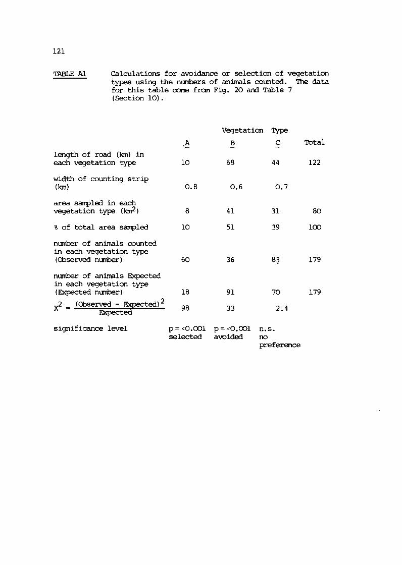
TmTJ3Al Calculations for avoidance or selection of vegetation types using the numbers of animals counted. The data for this table oorne fran Fig. 20 and Table 7 (Section 10).
Vegetation Type
A - B - c - Total
length of road (km) in each vegetation type 10 6 8 44 122
width of counting strip (k.1 0.8 0.6 0.7
area sampled in each vegetation type (krn2) 8 4 1 3 1 80
% of total area sampled 10 5 1 39 100
number of animals counted in each vegetation type (Observed number) 60 3 6 83 179
number of animals Expected in each vegetation type (Expected number) 18 9 1 70 179
significance level p=<O.OOl p=c0.001 n.s. selected avoided no
preference

18 animals are Expected in Type - A because Type - A comprised 10% of the
whole sample) . The I? value for each vegetation type is given by
- any I? of more than 3.841 being significant at the 5% level (for
there is only 1 degree of freedom). The results in Table 8 show
that the animals are selecting vegetation Type A (for the Observed - values are significantly higher than the Expected values) ; they are
avoiding Type B (for the Observed values are significantly less than - the Expected values), and they are shewing no particular avoidance or
preference for Type - C. This type of analysis has been used in a study of the
seasonal patterns of vegetation type use by large maimals in the
middle Zantezi valleyl1. The only drawback to the nethod is that it
is rather easy to obtain significant results, especially when the
observed numbers are large. Perhaps, therefore, the 1% level of
significance should be used, rather than the 5%.
(iii) methods using the density of anhnals
The best methods to use from the statistical viewpoint are
those that rely on the Observed densities of animals in each
vegetation type. The null hypothesis here is that if the animals
are distributed randanly with respect to the vegetation types, then
their density in each vegetation type would be the same. This null
hypothesis is tested by ccnparing the observed densities against the
mean density in the whole area surveyed.
The first step is to calculate the density in each sample
unit, or portion thereof, in each of the vegetation types. If grid
squares have been used as sample units, then the density refers to
each square. If transects have been used, then the density is
calculated from the portions of the transects in each vegetation
type. Thus, in Fig. A1 a) , the densities of animals would be found for each portion of the transects in each vegetation type, dl, dy,
d3 etc.
The most straightforward analysis is to use a simple one-way 1 analysis of variance such as that given in Bailey and as used by

tforton-~riffiths. he advantage of this analysis is that it is very
simple to carry out, and in addition one single set of calculations
enables you to compare the density in each vegetation type against the
overall mean density as well as the densities in each vegetation type
against each other. Once you have become used to handling a one-way I f
analysis of variance, you can graduate to two-way analysis 1 ,lO,24 I which tests a number of species and a number of vegetation types, or
a three-way analysis (which tests species, vegetation types and
seasons of the year).
Alternatively the analysis can be done in a slightly mre
laborious way by calculating the density and variance in each
vegetation type and the mean overall density, and then testing these 1 against each other using a t test or d test . This is exactly
equivalent to using an analysis of variance method, but it takes
longer and it is easier to make mistakes.
1.5 Pollwing Known Animals
The literature is crammed with studies of movements and
distribution in which known animals have been followed. The animals
are known either by distinguishing features ( e . g . ear tears in
elephants); by marking with collars, ear clipping or ear tags; or by
affixing a radio transmitter and using radio location 12t14. me
basic methodology is to make systematic observations of the animal's
position (e.g. daily, weekly, monthly) and to plot these positions on
a map. These data give measurements of daily rates of movement, wet
and dry season ranges, movements to and fran water, hone ranges,
territories and vegetation type utilisation.
The data tell a great deal about the movements of an individual
but not necessarily about the movements of a population or of a
seqment of a population. Of course, if you follow a marked animal in
a herd, then the whole herd is effectively marked. Usually, however,
the information on individuals' movements is used to auqment
information on a population's movement.
REFERENCES CITED FOR APPENDIX 1
1 Bailey, N.T.J. 1959 Statistical Methods in Biology. English Universities Press, London.
2 Bayliss, S.R. 1969 Winter food habits, range use and home range of antelope in Montana. J. Wildl. Manage. 33 (3) ,538-551 -
3 Caughley, G., Sinclair, R.G. & Wilson, G.R. 1977 Numbers, distribution and harvesting rate of kangaroos on the Inland Plains of New South Wales. Aust. Wildl. Res. - 4, 99-108
4 Duncan, P. 1975 Topi and their food supply. Ph. D. Thesis : University of Nairobi.
5 Field, C.R. & Laws, R.M. 1970 The distribution of the larger herbivores in the Queen Elizabeth National Park, Uqanda. J. appl. Ecol. 7, 273-294 -
6 Gittins, R. 1968 Trend surface analysis of ecological data. J. D l . 65 (3) , 845-869 -
7 Gwynne, M.D. & Smith, K. 1974 Proposals for the Boni Forest game reserve. Cyclostyled MS. Kenya Game Department , Nairobi.
8 Gwynne, M.D. & Croze, H.J. 1975a East African habitat monitoring practice : a review of methods and application. Proc. Synp. Evaluation and Mapping of Rangeland in Tropical Africa. I.L.C.A., Bamako, Mali. pp. 95-135
9 Gwynne, M.D. & Croze, H.J. 1975b The concept and practice of ecological mnitorinq over large areas of land : the systematic reconnaissance flight (SRF). Proc. Ibadan/Garoua International Symposium on Wildlife Management in Savanna Woodland, University of Ibadan, Nigeria.
10 Huitson, A. 1966 The Analysis of Variance. Griffin's Statistical Monoqraphs, No. 18. Charles Griffin, London.
11 Jannan, P.J. 1972 Seasonal distribution of large manma1 populations in the unflooded middle Zantoezi valley. J. appl. Ecol. - 9, 283-299
12 Kruuk, H. 1972 TTie Spotted Hyena. University of Chicaqo Press, Chicago.
13 Lamprey, H.F. 1963 Ecological separation of the large manma1 species in the Tarangire Game Reserve, Tanganyika. E. Afr. Wildl. J. 1, 1-30 -
14 Leuthold, W. & Sale, J.B. 1973 Movements and patterns of habitat utilisation of elephants in Tsavo National Park, Kenya. E. Afr. Wildl. J. 11, 369-384 -
15 Martinka, C.J. 1968 Habitat relationships of white-tailed deer and mule deer in northern -Montana. J. Wildl. Manage. 32 (3) , 558-565 -
16 Martinka, C.J. 1969 Population ecology of sunnier resident elk in Jackson Hole, Wyaning. J. Wildl. Manage. - 33(3), 465-481
17 Norton-Griffiths, M. 1975 The numbers and distribution of l q e mamnals in Ruaha National Park, Tanzania. E. Mr. Wildl. J. - 13, 121-140
18 Pennycuick, C.J., Sale, J.B., Stanley Price, M. & Jolly, G.M. 1977 Aerial systematic sampling applied to censuses of large mama1 populations in Kenya. E. Afr. Wildl. J. - 15, 139-146
Pennycuick, L. 1975 Movements of the migratory wildebeest population in the Serengeti area between 1960 and 1973. E. Afr. Wildl. J. - 13, 65-87
Pielou, E.C. 1966 An Introduction to Mathematical Ecology. John Wiley , London.
Sinclair, A.R.E. 1970 Studies of the ecology of the East African buffalo. Ph. D. Thesis, Oxford University.
Sinclair, A.R.E. 1974 Ttie natural regulation of buffalo populations in East Africa 1 : Introduction and resource requirements. E. Afr. Wildl. J. - 12, 135-154
Sinclair, A.R.E. 1977 The African Buffalo. Chicaqo University Press, Chicago.
Sokal, R.R. & Rohlf, F.J. 1969 Biometry. W.H. Freeman, San Francisco.
Southwood, T.R.E. 1966 Ecological Methods. Methuin, London.
Stevens, D.R. 1966 Range relationships of elk and livestock, Craw Creek Drainage, Fbntana. J. Wildl . Flanaqe. 30 (2) , - 349-363
Western, D. 1973 The Structure, Dynamics and Changes of the Amboseli Ecosystem. Ph.D. Thesis, University of Nairobi.
Western, D. 1976 The Distribution of Animals in Relation to Resources. Handbook No. 2, Techniques in African Wildlife Ecology. African Wildlife Leadership Foundation, Nairobi.
Western, D. 1976 An aerial method of monitoring large mammals and their environment, with a description of a computer program for survey analysis. Project Working Document 9, UNDP/FAO Kenya Wildlife Management Project (KEN/71/526) , Nairobi.

APPENDIX 2 TRAINING OBSERVERS
It is really quite extraordinary that aroonq the numerous
articles and publications about the techniques for counting animals
there appears to be not a single one devoted to training observers,
either for ground observation or for aerial observation. Quite
obviously, most observers have sinply 'grown into' their jobs, first
by being passengers in vehicles or aircraft, then perhaps by
standing-in when a more experienced observer was unavailable, and
finally. by deciding that they know what it is all about.
This dearth of information as to how to go about training
observers was sharply highlighted recently when the Kenya Ranqeland
Ecological Monitoring Unit (based in Nairobi, Kenya) was faced with
the task of training a cadre of eight Kenyan aerial observers from
scratch. None of the recruits had been in an aircraft, most had
never seen one close to, and few had ever encountered the larqe
mammals conrnon to Kenya's rangeland areas. Nevertheless, within
three months these trainee observers had reached a level of
performance equal to that of the mst experienced aerial observers
that could be found to test then against.
A full account of this training prograrrtne is in the process of
preparation, so only the most salient points will be qiven here as
a guideline.
The census method adopted by KREMU was essentially the same as
that described in Appendix 1, and the task facing their observers
was exacting. They had to spot, identify and count all animals
within their transact strip, photograph large groups and record all
these data unambiguously onto their tape recorders, alonq with
flight-line and sample-unit information. After each flight the
observers had to transcribe their tape records onto data sheets
and later match the photoqraohs to these tape records. Finally, they
had to analyse the photographs and count the animals on thorn and then
amend the tape records.
The training programs was built around a series of exercises
of increasing conplexity, each one introducing a new task to those
already learned. On the first exercise the observers were taught
simply to locate and identify animals; then to write down their
sightings; then to count the animals and write down the numbers; then
to use tape recorders; and finally to use cameras. The duration of
the flights was steadily increased as the course progressed until a
standard census flight of three hours was achieved.
Pre-flight, laboratory sessions gave opportunity to explain the
exercises, to practise with tape recorders and cameras, and to teach
operational procedures. Extensive, post-fliqht debriefinqs were used
for working up the data, for transcribinq and checking the tape
records and for analysing and counting the photographs.
Colour slides were used extensively throuqhout the course. They
were particularly useful for teachinq species identification, typical
habitat and group sizes, and techniques for scanninq , locating and counting groups of different sizes.
Perhaps the most useful teachinq aid durinq the course was the
intercom system fitted in the aircraft. The instructor, who was
sitting alonqside the pilot, was able to examine the same strip as the
observer imnediately behind him and could thus check on his
identification and on his countinq. Furthermore, the instructor could
listen-in while the observer was makino his tape record and could thus
check on his accuracy. Every half hour or so the two observers were
made to switch positions so that the instructor could interact with
both.
Table A2 shews the sequence of the exercises in this course and
the approximate number of hours spent by the observers on the various
activities.
A sumnary of the observer traininq programme is qiven below :
Exercise 1 : Pre-fliqht simple operational procedures; introduction to the aircraft, seatinq, seat belts, intercoms, location of survival qear
Flight writing d m date, name, side of aircraft, take off time, landing tine; spotting and identifying animals; pilot flies from qroup to group, circles group if necessary
Post-fliqht discussion of exercise; checking of flight data

TABLE A2 Hours spent by the trainee observers in the various activities on the KREMU aerial observer traininq course
Exercise
mean duration
preflight flight per flight post-f light
2 +write down 2 3 Us 4
4 + tape recorders 6 8 2 16
5 + cameras
TOTAL 20 31 52
Exercise 2 : Pre-flight
Flight
Exercise 3 : Pre-f light
Flight
Exercise 4 : Pre-flight
Flight
Post-flight
Exercise 5 : Re-flight
Flight
Post-flight
Use of Colour Slides
practice with data sheets
spotting and identifying aniJnals; writing down observations; pilot still flies from group to group
checking flight data; simple distribution maps
practice with writing down flight-line and sub-unit information, and numbers
counting groups and writing down numbers; writing down flight-lines and sample units; pilot flies systematic flight path, calling out beginning and end of flight-lines and sample units
checking flight-line, sample unit and other operational data; summarising numbers seen; simple distribution maps and population estimates
extensive practice in use of tape recorders; practice at transcribing prerecorded tapes onto computerised data sheets; operational procedures and checks of the tape recorders
counting animals within transect strip; recording data onto tape, alonq with all operational data
transcribing tape records onto data sheets; checking tape records.
extensive instruction in use of motor drive cameras, reloading, operational checks, use of automatic exposure control etc.
photographing all larqe groups and recordinq data; recordinq all other data as well
films developed; tapes transcribed; matching photographs to tape records; working out areas of overlap; counting photographs; amending data sheets; discussion of photo technique
A larqe number of 35 nm colour slides of animals were taken from
the normal operatinq height and sighting angle. Transect rods often
appear in the slides. The main uses were :- * identification of species in typical habitats and group sizes * techniques of scanninq and locatinq animals
* techniques for countinq large groups * appearance of same sized groups at different distances * appearance of different sized qroups at same distances * estimating proportion of a group inside the counting strip
* multi-species groups
In a standard session with colour slides, thirty six were
projected for ten seconds each, and the observers had to write down
the species and the nuinbers. The slides were then repeated, slowly,
and the instructor discussed each slide with the observers.

APPENDIX 3 M3RE ABOUT COUNTING BIAS
An extensive literature is new qrowing up about the main sources
of caunting bias in aerial suveys and on the ways to estimate and counteract their influence. The most recent and inportant work is
2 that of Caughley who, in a series of carefully designed experiments
in Australia, explored the effects of a number of factors on the densities of animals recorded by observers.
Caughley found that in general the most significant factors were
those of aircraft speed, aircraft height above ground and strip width;
others such as time of day, fatigue and length of survey appearing to
be less important. Furthermore, there was relatively little
interaction between these main sources of bias. Over the ranges
measured by him, speed and width were each effectively having a linear
and additatlve influence on sightability, while height was having a
parablic and U t a t i v e influence.
Che objective of Caughley's experiments was to test his 1
previously stated hypothesis that a regression of observed density
on speed, height and strip width could be extrapolated backwards to
the y-intercept to give an estimate of 'true density', at the zero
values of these variables. The experiJnenta1 results generally
favoured his hypothesis, and assuredly the estimates based on the
y-intercept were nearer to the ' true density' than were the unaided visual ones.
In a subsequent census of karwaroos3, Caughley used the
experimentally derived y-intercepts as correction factors for the
observed densities. Indeed, each observer had two correction factors, to take into account the density of the vegetation.
Undoubtedly, these studies of Caughley must now be taken very
seriously when designing census work. They demonstrate the
inadvisability of using fast census speeds and wide strip widths, until
recently quite the fashion. Furthermore, they demonstrate methods for
adjusting the results from censuses carried out in his way. And they W c a t e that the now anmnplace ~ ~ s e amng census operators in
East Africa of 100 I@ air speed, 300 feet height and a maximum of
150 metres strip width is along the right lines.

But a word of caution before speeds are reduced and heights
lowered. A recent tragic accident in Kenya, in which the whole crew
of a census aircraft was killed, has made those of us interested in
enjoying our dotage think seriously of four hundred feet as a
minimum, safe operating height.
Caughley's work still leaves a number of questions unresolved.
For example, occasionally other factors such as time of day would
have a highly significant effect on observed density. It was also
clear that the nature of the relationships between the main factors
and the observed densities changed with animal density, with species,
with vegetation and occasionally with individual observers.
Cauqhley recognises that his approach is best suited to censuses
of single species in relatively uniform habitats. The situation
becomes most ccmplicated where there is marked heterogeneity in
density, species, habitat and distribution, as is cannon in most East
African, multi-species censuses. Correction factors may well have to
be found for each combination, an awsane task only practicable under
circumstances where lonq-term work is being carried out.
In most Fast African census work, observers have been trained to
take photographs of all large groups (larger than ten animals) rather 4
than to try and guesstimate them . TTlis considerably reduces counting bias, although certain individual observers of long standing experience
consistently quesstimate with very little bias the nunber of animals
counted later from their photographs. Furthermore, in the East
African situation often as many as 95% of the total number of a
species counted will be on the photographs. The m i n i n g proportion
may scarcely warrant the expense of obtaininq correction factors. 5 This may explain why, in at least one East African study , factors
appearing un-rtant in Caughley's experjunents appeared to be
significantly associated with counting bias.
There are two further technical pints that must be considered.
First, the behaviour of the regression lines close to the y-intercept
is almost impossible to investiqate experimentally because of safety
aspects - although a helicopter could be employed for this. It is
likely that the reqression lines curve sharply in towards the
y-intercept in the region of, say, 5 - 25 feet height and 5 - 25 metres
strip width and 5 - 25 mph speed. Changes of these magnitudes in the
main factors may have little effect on sightability. In which case
the y-intercepts as calculated will overestimate the 'true density'.
Second, there is an error term, often as high as 35%, attached
to the y-intercept estimate. I am not sure at this stage what
should be done with it, but it cannot be ignored. It must contribute,
perhaps substantially, to the overall error of the estimate.

REFERENCES CITED FOR APPENDIX 3
1 Caughley, G. 1974 Bias in aerial survey. J. Wildl. Manage. 38 (4) , 921-933 -
2 Caughley, G., Sinclair, R.G. &,Scott-Kemnis, D. 1976 ExperiJnents in aerial survey. J. Wildl. Manage. - 40(2), 290-300
3 Caughley, G., Sinclair, R.G. & Wilson, G.R. 1977 Niinbers, distribution and harvesting rate of kangaroos on inland plains of New South Wales. Aust. Wildl. Res. - 4, 99-108
4 Norton-Griffiths, M. 1974' Reducing countin9 bias in aerial survey by using photography. E. Mr. Wildl. J. - 12(3), 245-248
5 Norton-Griffiths, M. 1976 Further aspects of bias in aerial census of large raamnals. J. Wildl. Manage. - 40(2), 368-370

APPENDIX 4 OPERATIONAL PROCEDURES AND CHECK SHEETS FOR CENSUSES
4.1 Introduction
Although aimed primarily at aerial survey crews, the following
operational procedures and check sheets should prove of value to
anyone setting out on census work. These lists are by no means
exhaustive, and individual census operators will undoubtedly amend
than to fit their particular requirements.
pilot
aircraft and equipment operational survival gear on board air/ground rescue co-ordination check maps and flight lines check order in which to fly flight lines stop watch and spare pens, pencils
front-seat recorder
check maps and flight lines check adequate data sheets, clip board check stop watch and spare pens, pencils, ear plugs (cotton wool)
rear-seat observers
check tape recorder working, record/play back check batteries and spares check tapes unrecorded, and spares pack recorder, tapes, batteries into flight bag ear plugs check camera operation, wind on, shutter operation check battery levels if appropriate check lens taped to infinity check ASA set correctly check shutter setting check exposure setting, operation check all films labelled on trailer, cassette and detachable sticky label
load film, check w i n d on stick label onto outside of camera load camera, spare films, batteries into flight bag
It is advisable to carry at least one spare camera and one
spare tape recorder on every flight.
Each camera and each tape recorder should have a unique
nunber so that malfunctioning equipment can be identified.
: When loading film, especially in the aircraft, the following
procedures are reccmnended :
check leader fully taken up of sprocket holes enqaqed
check normal wind on (twice) close back, check locked
into wind-on spool and both sets - with camera back open
wind on three times, checking counter and spol - (d) pre-flight briefing of all crew
objective of census flight plan recording methods pilot calling-out methods procedures if tape/cameras fail procedure if tape/caniera runs out during flight line emergency procedures, location of survival gear ground/air rescue co-ordination
(e) pre-flight
front-seat recorder write down onto data sheet :
date, name, fliqht code pilot's name observer LEFT and observer RIGHT aircraft identification
rear-seat observers record onto tape :
date, name, position (L/R), flight code, camera nuniber, tape recorder number tape number film number in camera (it's on the sticky label)
rear-seat observers play back tape recorder
rear-seat observers check camera operation, ASA, shutter, lens
4.3 In-flight
(a) pilot
record take off time give weaning of run-in to start of flight line call out "flight line NUMBER" check with all crew inembers that flight line number is correctly recorded
call "start of flight line NOW" call "sanple unit NUMBERw call "end of flight line NOW" call "BREAK" if flight line is to be stopped temporarily
Note : break either at end of sample unit, or at convenient land mark;
record landing time.

f ront -seat recorder
record t a k e o f f t ime w r i t e d m f l i g h t line number, check with p i l o t w r i t e down start time of f l i g h t line w r i t e down number of sanple u n i t record observat ions record radar a l t i m e t e r when p i l o t NOT lookina w r i t e dcwn next sample u n i t number w r i t e down end of t r a n s e c t t ime record landing tine
rear-seat observers
record f l i g h t line number, play back, check with p i l o t record sample u n i t number record observat ions record photoqraphic information record "end of f l i q h t l i n e number"
between t r a n s e c t s
check t ape recorder still working, b a t t e r i e s , tape to run check camera still workinq, f i lm counter , &A, exposure,
l e n s , s h u t t e r
changing t a p e s
record t a p e number, p lay back record d a t e , name, p o s i t i o n , f l i g h t code, f i l m in
camera, play back
chanqinq f i lms
rewind f u l l y into c a s s e t t e , unload remove detachable label f run camera, des t roy rerrove detachable label from new c a s s e t t e , s t i c k on to
camera load f i lm, check wind on check a l l camera opera t ions record new f i l m number on to tape play back and check
changing t a p e recorder or camera
record new t a p e recorder and/or camera number o n t o t a p e record reasons f o r change, new t a p e number, new f i l m
number etc.
I f poss ib le , change f i l m s and t a p e s between f l i g h t l i n e s . I f
caught s h o r t , ask p i l o t t o break f l i g h t l i n e as soon a s
poss ib le .
Say into recorder "elephant , e lephant , seven"; t h i s g i v e s the
recorder time t o g e t t o f u l l speed a f t e r switching on.
Say into recorder "cor rec t ion , co r rec t ion . . I 8 i f an observation
is t o be changed.

: Rananrber ALWAYS to take photoqraphs with the camera near
vertical and NOT horizontal. If Horizontal, effective eye
position is lowered, and more animals are included into the
viewing strip.
4.4 Post-Flight
pilot
tend to aircraft record flight times, census zone, flight line numbers into aircraft journey log book and into personal loq book
rear-seat observers
transcribe tape records onto data sheets check through again carefully match film and tape numbers to transcription match camera and tape recorder numbers to transcription put used tapes and films away safely threw away used batteries, spoilt cassettes etc.
frcnt-seat observer
tidy up data sheets
crew debriefing
recorder and observers match flight line numbers and sample unit numbers
clear up any mistakes while -ry is still fresh label and pack together all data sheets, films, tapes discuss census operation plan next f 1 ight
It is most advisable to keep tapes until the census data are
fully processed. Often you will find difficulties with
matching the tape transcripts with the photoqraphic record.
Access to the original tape record is then very useful.
4.5 Setting Up and Calibrating Transect Streamers
(a) setting up
follow procedures outlined on Page 53; requirements wax pencils, tape measure.
write down for future reference
observer's name and height aircraft identification side of aircraft height of observer's eye above the ground when sitting ins ide

height on upper and lower window marks distance of inner and outer streamer from fuselage
(b) markers
lay out brightly whitened mrkers in a straight line along runway - small markers every 20 metres; large marker every 100 metres
calibration
pilot flies across line of markers
at right angles to them at census height and at census speed (or slcwer) with aircraft level and no bank
front-seat recorder fixates on radar altimter rear-seat observer counts markers between streamers rear-seat observer shouts "NOW" as the markers pass by front-eat recorder writes dmn reading of radar altimeter rear-seat observer calls out number of markers front-seat recorder writes down number, and checks
Repeat at least five tiroes for each observer.
Repeat at two other heights, 100 feet above and 100 feet
below census height.
(d) calculations
calculate strip width for nominal census height repeat procedures if strip width too far from planned width calculate correction factor for height above ground record this along with data itemised under (a) above
Notes : It is advisable not to use cameras for counting the markers
between the streamers. Difficulties in taking the photos
frun exactly the correct posision tend to invalidate the
results . : most census operators now use fishing rods (glass fibre) set Into strong wooden clanps to demarcate the strip. The
clairpe are shaped to fit over the wing struts and are
rencvable. Spare bolts, wing nuts and spring washers for
the clamps should be carried in the aircraft. Trie rods
should be painted with white rings so that they show up
width, mark position of clanps with paint. This indicates
if they slip during the flight.

- - -. - -- - - - - -- - -- -- -- - - - --- - - - --- Printed by Afroprcts Ltd., Lusaka Close, off Luaaka Road, P.O. Box 30502. Nairobi, Kenya