
REVIEW OF DIFFERENTIATIONmathminer.org/files/Zill_8th_ch1-3.pdf · with Boundary-Value Problems...
165
Transcript of REVIEW OF DIFFERENTIATIONmathminer.org/files/Zill_8th_ch1-3.pdf · with Boundary-Value Problems...


REVIEW OF DIFFERENTIATION
a a a
a a
Copyright 2012 Cengage Learning. All Rights Reserved. May not be copied, scanned, or duplicated, in whole or in part. Due to electronic rights, some third party content may be suppressed from the eBook and/or eChapter(s).
Editorial review has deemed that any suppressed content does not materially affect the overall learning experience. Cengage Learning reserves the right to remove additional content at any time if subsequent rights restrictions require it.

BRIEF TABLE OF INTEGRALS
Copyright 2012 Cengage Learning. All Rights Reserved. May not be copied, scanned, or duplicated, in whole or in part. Due to electronic rights, some third party content may be suppressed from the eBook and/or eChapter(s).
Editorial review has deemed that any suppressed content does not materially affect the overall learning experience. Cengage Learning reserves the right to remove additional content at any time if subsequent rights restrictions require it.

Eighth Edition
DIFFERENTIALEQUATIONSwith Boundary-Value Problems
Copyright 2012 Cengage Learning. All Rights Reserved. May not be copied, scanned, or duplicated, in whole or in part. Due to electronic rights, some third party content may be suppressed from the eBook and/or eChapter(s).
Editorial review has deemed that any suppressed content does not materially affect the overall learning experience. Cengage Learning reserves the right to remove additional content at any time if subsequent rights restrictions require it.

Eighth Edition
DIFFERENTIALEQUATIONS with Boundary-Value Problems
DENNIS G. ZILLLoyola Marymount University
WARREN S. WRIGHTLoyola Marymount University
MICHAEL R. CULLENLate of Loyola Marymount University
Australia • Brazil • Japan • Korea • Mexico • Singapore • Spain • United Kingdom • United States
Copyright 2012 Cengage Learning. All Rights Reserved. May not be copied, scanned, or duplicated, in whole or in part. Due to electronic rights, some third party content may be suppressed from the eBook and/or eChapter(s).
Editorial review has deemed that any suppressed content does not materially affect the overall learning experience. Cengage Learning reserves the right to remove additional content at any time if subsequent rights restrictions require it.

This is an electronic version of the print textbook. Due to electronic rights restrictions,some third party content may be suppressed. Editorial review has deemed that any suppressed content does not materially affect the overall learning experience. The publisher reserves the right to remove content from this title at any time if subsequent rights restrictions require it. Forvaluable information on pricing, previous editions, changes to current editions, and alternate formats, please visit www.cengage.com/highered to search by ISBN#, author, title, or keyword for materials in your areas of interest.
Copyright 2012 Cengage Learning. All Rights Reserved. May not be copied, scanned, or duplicated, in whole or in part. Due to electronic rights, some third party content may be suppressed from the eBook and/or eChapter(s).
Editorial review has deemed that any suppressed content does not materially affect the overall learning experience. Cengage Learning reserves the right to remove additional content at any time if subsequent rights restrictions require it.

Differential Equations withBoundary-Value Problems,Eighth EditionDennis G. Zill, Warren S. Wright,and Michael R. Cullen
Publisher: Richard Stratton
Senior Sponsoring Editor:Molly Taylor
Development Editor: Leslie Lahr
Assistant Editor:Shaylin Walsh Hogan
Editorial Assistant: Alex Gontar
Media Editor: Andrew Coppola
Marketing Manager: Jennifer Jones
Marketing Coordinator:Michael Ledesma
Marketing Communications Manager:Mary Anne Payumo
Content Project Manager:Alison Eigel Zade
Senior Art Director: Linda May
Manufacturing Planner: Doug Bertke
Rights Acquisition Specialist:Shalice Shah-Caldwell
Production Service: MPS Limited,a Macmillan Company
Text Designer: Diane Beasley
Projects Piece Designer:Rokusek Design
Cover Designer:One Good Dog Design
Cover Image: ©Wally Pacholka
Compositor: MPS Limited,a Macmillan Company
Section 4.8 of this text appears inAdvanced Engineering Mathematics,Fourth Edition, Copyright 2011,Jones & Bartlett Learning, Burlington,MA 01803 and is used with thepermission of the publisher.
© 2013, 2009, 2005 Brooks/Cole, Cengage Learning
ALL RIGHTS RESERVED. No part of this work covered by thecopyright herein may be reproduced, transmitted, stored, or used inany form or by any means graphic, electronic, or mechanical,including but not limited to photocopying, recording, scanning,digitizing, taping, Web distribution, information networks, orinformation storage and retrieval systems, except as permitted underSection 107 or 108 of the 1976 United States Copyright Act, withoutthe prior written permission of the publisher.
Library of Congress Control Number: 2011944305ISBN-13: 978-1-111-82706-9ISBN-10: 1-111-82706-0
Brooks/Cole20 Channel Center StreetBoston, MA 02210USA
Cengage Learning is a leading provider of customized learning solutions with office loc tions around the globe, including Singapore,the United Kingdom, Australia, Mexico, Brazil and Japan. Locateyour local office t international.cengage.com/region
Cengage Learning products are represented in Canada by NelsonEducation, Ltd.
For your course and learning solutions, visitwww.cengage.com.
Purchase any of our products at your local college storeor at our preferred online store www.cengagebrain.com.Instructors: Please visit login.cengage.com and log in to accessinstructor-specific resource .
For product information and technology assistance, contact us atCengage Learning Customer & Sales Support, 1-800-354-9706
For permission to use material from this text or product,submit all requests online at www.cengage.com/permissions.
Further permissions questions can be emailed to [email protected].
Printed in the United States of America1 2 3 4 5 6 7 16 15 14 13 12
Copyright 2012 Cengage Learning. All Rights Reserved. May not be copied, scanned, or duplicated, in whole or in part. Due to electronic rights, some third party content may be suppressed from the eBook and/or eChapter(s).
Editorial review has deemed that any suppressed content does not materially affect the overall learning experience. Cengage Learning reserves the right to remove additional content at any time if subsequent rights restrictions require it.


3
v
Contents
1 INTRODUCTION TO DIFFERENTIAL EQUATIONS 1
Preface xi
Projects P-1
1.1 Definitions and Terminology 2
1.2 Initial-Value Problems 13
1.3 Differential Equations as Mathematical Models 20
Chapter 1 in Review 33
2 FIRST-ORDER DIFFERENTIAL EQUATIONS 35
2.1 Solution Curves Without a Solution 36
2.1.1 Direction Fields 36
2.1.2 Autonomous First-Order DEs 38
2.2 Separable Equations 46
2.3 Linear Equations 54
2.4 Exact Equations 63
2.5 Solutions by Substitutions 71
2.6 A Numerical Method 75
Chapter 2 in Review 80
MODELING WITH FIRST-ORDER DIFFERENTIAL EQUATIONS 83
3.1 Linear Models 84
3.2 Nonlinear Models 95
3.3 Modeling with Systems of First-Order DEs 106
Chapter 3 in Review 113
Copyright 2012 Cengage Learning. All Rights Reserved. May not be copied, scanned, or duplicated, in whole or in part. Due to electronic rights, some third party content may be suppressed from the eBook and/or eChapter(s).
Editorial review has deemed that any suppressed content does not materially affect the overall learning experience. Cengage Learning reserves the right to remove additional content at any time if subsequent rights restrictions require it.

5
4
vi CONTENTS
HIGHER-ORDER DIFFERENTIAL EQUATIONS 116
4.1 Preliminary Theory—Linear Equations 117
4.1.1 Initial-Value and Boundary-Value Problems 117
4.1.2 Homogeneous Equations 119
4.1.3 Nonhomogeneous Equations 124
4.2 Reduction of Order 129
4.3 Homogeneous Linear Equations with Constant Coefficient 132
4.4 Undetermined Coefficients—Superposition Approach 139
4.5 Undetermined Coefficients—Annihilator Approach 149
4.6 Variation of Parameters 156
4.7 Cauchy-Euler Equation 162
4.8 Green’s Functions 169
4.8.1 Initial-Value Problems 169
4.8.2 Boundary-Value Problems 176
4.9 Solving Systems of Linear DEs by Elimination 180
4.10 Nonlinear Differential Equations 185
Chapter 4 in Review 190
MODELING WITH HIGHER-ORDER DIFFERENTIAL EQUATIONS 192
5.1 Linear Models: Initial-Value Problems 193
5.1.1 Spring/Mass Systems: Free Undamped Motion 193
5.1.2 Spring/Mass Systems: Free Damped Motion 197
5.1.3 Spring/Mass Systems: Driven Motion 200
5.1.4 Series Circuit Analogue 203
5.2 Linear Models: Boundary-Value Problems 210
5.3 Nonlinear Models 218
Chapter 5 in Review 228
SERIES SOLUTIONS OF LINEAR EQUATIONS 231
6.1 Review of Power Series 232
6.2 Solutions About Ordinary Points 238
6.3 Solutions About Singular Points 247
6.4 Special Functions 257
Chapter 6 in Review 271
6
Copyright 2012 Cengage Learning. All Rights Reserved. May not be copied, scanned, or duplicated, in whole or in part. Due to electronic rights, some third party content may be suppressed from the eBook and/or eChapter(s).
Editorial review has deemed that any suppressed content does not materially affect the overall learning experience. Cengage Learning reserves the right to remove additional content at any time if subsequent rights restrictions require it.

CONTENTS vii
7 THE LAPLACE TRANSFORM 273
7.1 Definition of the Laplace Transform 274
7.2 Inverse Transforms and Transforms of Derivatives 281
7.2.1 Inverse Transforms 281
7.2.2 Transforms of Derivatives 284
7.3 Operational Properties I 289
7.3.1 Translation on the s-Axis 290
7.3.2 Translation on the t-Axis 293
7.4 Operational Properties II 301
7.4.1 Derivatives of a Transform 301
7.4.2 Transforms of Integrals 302
7.4.3 Transform of a Periodic Function 307
7.5 The Dirac Delta Function 312
7.6 Systems of Linear Differential Equations 315
Chapter 7 in Review 320
8 SYSTEMS OF LINEAR FIRST-ORDER DIFFERENTIAL EQUATIONS 325
8.1 Preliminary Theory—Linear Systems 326
8.2 Homogeneous Linear Systems 333
8.2.1 Distinct Real Eigenvalues 334
8.2.2 Repeated Eigenvalues 337
8.2.3 Complex Eigenvalues 342
8.3 Nonhomogeneous Linear Systems 348
8.3.1 Undetermined Coefficient 348
8.3.2 Variation of Parameters 351
8.4 Matrix Exponential 356
Chapter 8 in Review 360
9 NUMERICAL SOLUTIONS OF ORDINARY DIFFERENTIAL EQUATIONS 362
9.1 Euler Methods and Error Analysis 363
9.2 Runge-Kutta Methods 368
9.3 Multistep Methods 373
9.4 Higher-Order Equations and Systems 375
9.5 Second-Order Boundary-Value Problems 380
Chapter 9 in Review 384
Copyright 2012 Cengage Learning. All Rights Reserved. May not be copied, scanned, or duplicated, in whole or in part. Due to electronic rights, some third party content may be suppressed from the eBook and/or eChapter(s).
Editorial review has deemed that any suppressed content does not materially affect the overall learning experience. Cengage Learning reserves the right to remove additional content at any time if subsequent rights restrictions require it.

viii CONTENTS
10 PLANE AUTONOMOUS SYSTEMS 385
10.1 Autonomous Systems 386
10.2 Stability of Linear Systems 392
10.3 Linearization and Local Stability 400
10.4 Autonomous Systems as Mathematical Models 410
Chapter 10 in Review 417
11 FOURIER SERIES 419
11.1 Orthogonal Functions 420
11.2 Fourier Series 426
11.3 Fourier Cosine and Sine Series 431
11.4 Sturm-Liouville Problem 439
11.5 Bessel and Legendre Series 446
11.5.1 Fourier-Bessel Series 447
11.5.2 Fourier-Legendre Series 450
Chapter 11 in Review 453
12 BOUNDARY-VALUE PROBLEMS IN RECTANGULAR COORDINATES 455
12.1 Separable Partial Differential Equations 456
12.2 Classical PDEs and Boundary-Value Problems 460
12.3 Heat Equation 466
12.4 Wave Equation 468
12.5 Laplace’s Equation 473
12.6 Nonhomogeneous Boundary-Value Problems 478
12.7 Orthogonal Series Expansions 483
12.8 Higher-Dimensional Problems 488
Chapter 12 in Review 491
Copyright 2012 Cengage Learning. All Rights Reserved. May not be copied, scanned, or duplicated, in whole or in part. Due to electronic rights, some third party content may be suppressed from the eBook and/or eChapter(s).
Editorial review has deemed that any suppressed content does not materially affect the overall learning experience. Cengage Learning reserves the right to remove additional content at any time if subsequent rights restrictions require it.

CONTENTS ix
13 BOUNDARY-VALUE PROBLEMS IN OTHER COORDINATE SYSTEMS 493
13.1 Polar Coordinates 494
13.2 Polar and Cylindrical Coordinates 499
13.3 Spherical Coordinates 505
Chapter 13 in Review 508
14 INTEGRAL TRANSFORMS 510
14.1 Error Function 511
14.2 Laplace Transform 512
14.3 Fourier Integral 520
14.4 Fourier Transforms 526
Chapter 14 in Review 532
15 NUMERICAL SOLUTIONS OF PARTIAL DIFFERENTIAL EQUATIONS 534
15.1 Laplace’s Equation 535
15.2 Heat Equation 540
15.3 Wave Equation 545
Chapter 15 in Review 549
APPENDIXES
I Gamma Function APP-1
II Matrices APP-3
III Laplace Transforms APP-21
Answers for Selected Odd-Numbered Problems ANS-1
Index I-1
Copyright 2012 Cengage Learning. All Rights Reserved. May not be copied, scanned, or duplicated, in whole or in part. Due to electronic rights, some third party content may be suppressed from the eBook and/or eChapter(s).
Editorial review has deemed that any suppressed content does not materially affect the overall learning experience. Cengage Learning reserves the right to remove additional content at any time if subsequent rights restrictions require it.

xi
TO THE STUDENT
Authors of books live with the hope that someone actually reads them. Contrary towhat you might believe, almost everything in a typical college-level mathematicstext is written for you, and not the instructor. True, the topics covered in the text arechosen to appeal to instructors because they make the decision on whether to use itin their classes, but everything written in it is aimed directly at you, the student. Sowe want to encourage you—no, actually we want to tell you—to read this textbook!But do not read this text like you would a novel; you should not read it fast and youshould not skip anything. Think of it as a workbook. By this we mean that mathemat-ics should always be read with pencil and paper at the ready because, most likely, youwill have to work your way through the examples and the discussion. Before attempt-ing any of the exercises, work all the examples in a section; the examples are con-structed to illustrate what we consider the most important aspects of the section, andtherefore, reflect the procedures necessary to work most of the problems in the exer-cise sets. We tell our students when reading an example, copy it down on a piece ofpaper, and do not look at the solution in the book. Try working it, then compare yourresults against the solution given, and, if necessary resolve, any differences. We havetried to include most of the important steps in each example, but if something is notclear you should always try—and here is where the pencil and paper come in again—to fill in the details or missing steps. This may not be easy, but that is part of the learn-ing process. The accumulation of facts followed by the slow assimilation of under-standing simply cannot be achieved without a struggle.
Specifically for you, a Student Resource Manual (SRM) is available as an op-tional supplement. In addition to containing solutions of selected problems from theexercises sets, the SRM contains hints for solving problems, extra examples, and a re-view of those areas of algebra and calculus that we feel are particularly important tothe successful study of differential equations. Bear in mind you do not have to pur-chase the SRM; by following my pointers given at the beginning of most sections, youcan review the appropriate mathematics from your old precalculus or calculus texts.
In conclusion, we wish you good luck and success. We hope you enjoy the textand the course you are about to embark on—as undergraduate math majors it wasone of our favorites because we liked mathematics that connected with the physicalworld. If you have any comments, or if you find any errors as you read/work yourway through the text, or if you come up with a good idea for improving either it orthe SRM, please feel free to contact us through our editor at Cengage Learning:
TO THE INSTRUCTOR
In case you are examining this book for the first time, Differential Equations withBoundary-Value Problems, Eighth Edition can be used for either a one-semester course,or a two-semester course that covers ordinary and partial differential equations. Theshorter version of the text, A First Course in Differential Equations with ModelingApplications, Tenth Edition, is intended for either a one-semester or a one-quarter coursein ordinary differential equations. This book ends with Chapter 9. For a one semestercourse, we assume that the students have successfully completed at least two semestersof calculus. Since you are reading this, undoubtedly you have already examined the
Preface
Copyright 2012 Cengage Learning. All Rights Reserved. May not be copied, scanned, or duplicated, in whole or in part. Due to electronic rights, some third party content may be suppressed from the eBook and/or eChapter(s).
Editorial review has deemed that any suppressed content does not materially affect the overall learning experience. Cengage Learning reserves the right to remove additional content at any time if subsequent rights restrictions require it.
table of contents for the topics that are covered. You will not find a “suggested syl-labus” in this preface; we will not pretend to be so wise as to tell other teachers what toteach. We feel that there is plenty of material here to pick from and to form a course toyour liking. The textbook strikes a reasonable balance between the analytical, qualita-tive, and quantitative approaches to the study of differential equations. As far as our“underlying philosophy” it is this: An undergraduate textbook should be written withthe student’s understanding kept firmly in mind, which means to me that the materialshould be presented in a straightforward, readable, and helpful manner, while keepingthe level of theory consistent with the notion of a “first course.
For those who are familiar with the previous editions, we would like to mentiona few of the improvements made in this edition.
• Eight new projects appear at the beginning of the book. Each project includesa related problem set, and a correlation of the project material with a chapterin the text.
• Many exercise sets have been updated by the addition of new problems tobetter test and challenge the students. In like manner, some exercise sets havebeen improved by sending some problems into retirement.
• Additional examples and figures have been added to many sections• Several instructors took the time to e-mail us expressing their concerns
about our approach to linear first-order differential equations. In response,Section 2.3, Linear Equations, has been rewritten with the intent to simplifythe discussion.
• This edition contains a new section on Green’s functions in Chapter 4 for thosewho have extra time in their course to consider this elegant application ofvariation of parameters in the solution of initial-value and boundary-value prob-lems. Section 4.8 is optional and its content does not impact any other section.
• Section 5.1 now includes a discussion on how to use both trigonometricforms
in describing simple harmonic motion.• At the request of users of the previous editions, a new section on the review
of power series has been added to Chapter 6. Moreover, much of this chapterhas been rewritten to improve clarity. In particular, the discussion of themodified Bessel functions and the spherical Bessel functions in Section 6.4has been greatly expanded.
• Several boundary-value problems involving modified Bessel functions havebeen added to Exercises 13.2.
STUDENT RESOURCES
• Student Resource Manual (SRM), prepared by Warren S. Wright and Carol D.Wright (ISBN 9781133491927 accompanies A First Course in DifferentialEquations with Modeling Applications, Tenth Edition, and ISBN 9781133491958accompanies Differential Equations with Boundary-Value Problems, EighthEdition), provides important review material from algebra and calculus, thesolution of every third problem in each exercise set (with the exception of theDiscussion Problems and Computer Lab Assignments), relevant commandsyntax for the computer algebra systems Mathematica and Maple, lists ofimportant concepts, as well as helpful hints on how to start certain problems.
INSTRUCTOR RESOURCES
• Instructor’s Solutions Manual (ISM) prepared by Warren S. Wright andCarol D. Wright (ISBN 9781133602293) provides complete, worked-outsolutions for all problems in the text.
• Solution Builder is an online instructor database that offers complete, worked-out solutions for all exercises in the text, allowing you to create customized,
y Asin(vt f) and y Acos(vt f)
xii PREFACE
Copyright 2012 Cengage Learning. All Rights Reserved. May not be copied, scanned, or duplicated, in whole or in part. Due to electronic rights, some third party content may be suppressed from the eBook and/or eChapter(s).
Editorial review has deemed that any suppressed content does not materially affect the overall learning experience. Cengage Learning reserves the right to remove additional content at any time if subsequent rights restrictions require it.

PREFACE xiii
secure solutions printouts (in PDF format) matched exactly to the problems youassign in class. Access is available via
www.cengage.com/solutionbuilder
• ExamView testing software allows instructors to quickly create, deliver, andcustomize tests for class in print and online formats, and features automaticgrading. Included is a test bank with hundreds of questions customized di-rectly to the text, with all questions also provided in PDF and MicrosoftWord formats for instructors who opt not to use the software component.
• Enhanced WebAssign is the most widely used homework system in highereducation. Available for this title, Enhanced WebAssign allows you to assign,collect, grade, and record assignments via the Web. This proven homeworksystem includes links to textbook sections, video examples, and problem spe-cific tutorials. Enhanced WebAssign is more than a homework system—it isa complete learning system for students.
ACKNOWLEDGMENTS
We would like to single out a few people for special recognition. Many thanks toMolly Taylor (senior sponsoring editor), Shaylin Walsh Hogan (assistant editor), andAlex Gontar (editorial assistant) for orchestrating the development of this edition andits component materials. Alison Eigel Zade (content project manager) offered theresourcefulness, knowledge, and patience necessary to a seamless production process.Ed Dionne (project manager, MPS) worked tirelessly to provide top-notch publishingservices. And finall , we thank Scott Brown for his superior skills as accuracy reviewer.Once again an especially heartfelt thank you to Leslie Lahr, developmental editor, forher support, sympathetic ear, willingness to communicate, suggestions, and forobtaining and organizing the excellent projects that appear at the front of the book.We also extend our sincerest appreciation to those individuals who took the time outof their busy schedules to submit a project:
Ivan Kramer, University of Maryland—Baltimore CountyTom LaFaro, Gustavus Adolphus CollegeJo Gascoigne, Fisheries ConsultantC. J. Knickerbocker, Sensis CorporationKevin Cooper, Washington State UniversityGilbert N. Lewis, Michigan Technological UniversityMichael Olinick, Middlebury College
Finally, over the years these textbooks have been improved in a countless num-ber of ways through the suggestions and criticisms of the reviewers. Thus it is fittinto conclude with an acknowledgement of our debt to the following wonderful peoplefor sharing their expertise and experience.
REVIEWERS OF PAST EDITIONS
William Atherton, Cleveland State University Philip Bacon, University of FloridaBruce Bayly, University of Arizona William H. Beyer, University of AkronR. G. Bradshaw, Clarkson CollegeDean R. Brown, Youngstown State University David Buchthal, University of AkronNguyen P. Cac, University of Iowa T. Chow, California State University—Sacramento Dominic P. Clemence, North Carolina Agricultural and Technical
State University Pasquale Condo, University of Massachusetts—Lowell
Copyright 2012 Cengage Learning. All Rights Reserved. May not be copied, scanned, or duplicated, in whole or in part. Due to electronic rights, some third party content may be suppressed from the eBook and/or eChapter(s).
Editorial review has deemed that any suppressed content does not materially affect the overall learning experience. Cengage Learning reserves the right to remove additional content at any time if subsequent rights restrictions require it.

Vincent Connolly, Worcester Polytechnic Institute Philip S. Crooke, Vanderbilt University Bruce E. Davis, St. Louis Community College at Florissant Valley Paul W. Davis, Worcester Polytechnic Institute Richard A. DiDio, La Salle University James Draper, University of Florida James M. Edmondson, Santa Barbara City CollegeJohn H. Ellison, Grove City College Raymond Fabec, Louisiana State University Donna Farrior, University of Tulsa Robert E. Fennell, Clemson University W. E. Fitzgibbon, University of Houston Harvey J. Fletcher, Brigham Young University Paul J. Gormley, Villanova Layachi Hadji, University of AlabamaRuben Hayrapetyan, Kettering UniversityTerry Herdman, Virginia Polytechnic Institute and State UniversityZdzislaw Jackiewicz, Arizona State University S. K. Jain, Ohio University Anthony J. John, Southeastern Massachusetts University David C. Johnson, University of Kentucky—LexingtonHarry L. Johnson, V.P.I & S.U. Kenneth R. Johnson, North Dakota State University Joseph Kazimir, East Los Angeles College J. Keener, University of Arizona Steve B. Khlief, Tennessee Technological University (retired) C. J. Knickerbocker, Sensis Corporation Carlon A. Krantz, Kean College of New Jersey Thomas G. Kudzma, University of Lowell Alexandra Kurepa, North Carolina A&T State UniversityG. E. Latta, University of Virginia Cecelia Laurie, University of Alabama James R. McKinney, California Polytechnic State UniversityJames L. Meek, University of Arkansas Gary H. Meisters, University of Nebraska—Lincoln Stephen J. Merrill, Marquette University Vivien Miller, Mississippi State University Gerald Mueller, Columbus State Community College Philip S. Mulry, Colgate University C. J. Neugebauer, Purdue University Tyre A. Newton, Washington State University Brian M. O’Connor, Tennessee Technological University J. K. Oddson, University of California—Riverside Carol S. O’Dell, Ohio Northern University A. Peressini, University of Illinois, Urbana—Champaign J. Perryman, University of Texas at Arlington Joseph H. Phillips, Sacramento City College Jacek Polewczak, California State University Northridge Nancy J. Poxon, California State University—Sacramento Robert Pruitt, San Jose State University K. Rager, Metropolitan State College F. B. Reis, Northeastern University Brian Rodrigues, California State Polytechnic UniversityTom Roe, South Dakota State UniversityKimmo I. Rosenthal, Union College Barbara Shabell, California Polytechnic State University Seenith Sivasundaram, Embry-Riddle Aeronautical University
xiv PREFACE
Copyright 2012 Cengage Learning. All Rights Reserved. May not be copied, scanned, or duplicated, in whole or in part. Due to electronic rights, some third party content may be suppressed from the eBook and/or eChapter(s).
Editorial review has deemed that any suppressed content does not materially affect the overall learning experience. Cengage Learning reserves the right to remove additional content at any time if subsequent rights restrictions require it.

Don E. Soash, Hillsborough Community College F. W. Stallard, Georgia Institute of Technology Gregory Stein, The Cooper Union M. B. Tamburro, Georgia Institute of Technology Patrick Ward, Illinois Central College Jianping Zhu, University of AkronJan Zijlstra, Middle Tennessee State University Jay Zimmerman, Towson University
REVIEWERS OF THE CURRENT EDITIONS
Bernard Brooks, Rochester Institute of TechnologyAllen Brown, Wabash Valley College Helmut Knaust, The University of Texas at El Paso Mulatu Lemma, Savannah State University George Moss, Union University Martin Nakashima, California State Polytechnic University—PomonaBruce O’Neill, Milwaukee School of Engineering
Dennis G. ZillWarren S. Wright
Los Angeles
PREFACE xv
Copyright 2012 Cengage Learning. All Rights Reserved. May not be copied, scanned, or duplicated, in whole or in part. Due to electronic rights, some third party content may be suppressed from the eBook and/or eChapter(s).
Editorial review has deemed that any suppressed content does not materially affect the overall learning experience. Cengage Learning reserves the right to remove additional content at any time if subsequent rights restrictions require it.

Is AIDS an Invariably Fatal Disease?by Ivan Kramer
This essay will address and answer the question: Is the acquired immunodeficiencsyndrome (AIDS), which is the end stage of the human immunodeficiency virus(HIV) infection, an invariably fatal disease?
Like other viruses, HIV has no metabolism and cannot reproduce itself outside ofa living cell. The genetic information of the virus is contained in two identical strandsof RNA. To reproduce, HIV must use the reproductive apparatus of the cell it invadesand infects to produce exact copies of the viral RNA. Once it penetrates a cell, HIVtranscribes its RNA into DNA using an enzyme (reverse transcriptase) contained in thevirus. The double-stranded viral DNA migrates into the nucleus of the invaded cell andis inserted into the cell’s genome with the aid of another viral enzyme (integrase). Theviral DNA and the invaded cell’s DNA are then integrated, and the cell is infected.When the infected cell is stimulated to reproduce, the proviral DNA is transcribed intoviral DNA, and new viral particles are synthesized. Since anti-retroviral drugs like zi-dovudine inhibit the HIV enzyme reverse transcriptase and stop proviral DNA chainsynthesis in the laboratory, these drugs, usually administered in combination, slowdown the progression to AIDS in those that are infected with HIV (hosts).
What makes HIV infection so dangerous is the fact that it fatally weakens ahost’s immune system by binding to the CD4 molecule on the surface of cells vitalfor defense against disease, including T-helper cells and a subpopulation of naturalkiller cells. T-helper cells (CD4 T-cells, or T4 cells) are arguably the most importantcells of the immune system since they organize the body’s defense against antigens.Modeling suggests that HIV infection of natural killer cells makes it impossible foreven modern antiretroviral therapy to clear the virus [1]. In addition to the CD4molecule, a virion needs at least one of a handful of co-receptor molecules (e.g., CCR5and CXCR4) on the surface of the target cell in order to be able to bind to it, pene-trate its membrane, and infect it. Indeed, about 1% of Caucasians lack coreceptormolecules, and, therefore, are completely immune to becoming HIV infected.
Once infection is established, the disease enters the acute infection stage, lastinga matter of weeks, followed by an incubation period, which can last two decades ormore! Although the T-helper cell density of a host changes quasi-statically during theincubation period, literally billions of infected T4 cells and HIV particles aredestroyed—and replaced—daily. This is clearly a war of attrition, one in which theimmune system invariably loses.
A model analysis of the essential dynamics that occur during the incubationperiod to invariably cause AIDS is as follows [1]. Because HIV rapidly mutates, itsability to infect T4 cells on contact (its infectivity) eventually increases and therate T4 cells become infected increases. Thus, the immune system must increase thedestruction rate of infected T4 cells as well as the production rate of new, uninfectedones to replace them. There comes a point, however, when the production rate of T4cells reaches its maximum possible limit and any further increase in HIV’s infectiv-ity must necessarily cause a drop in the T4 density leading to AIDS. Remarkably,about 5% of hosts show no sign of immune system deterioration for the first ten yearsof the infection; these hosts, called long-term nonprogressors, were originally
Project for Section 3.1
P-1
Cell infected with HIV
Tho
mas
Dee
rinc
k, N
CM
IR/P
hoto
Res
earc
hers
, Inc
.
Copyright 2012 Cengage Learning. All Rights Reserved. May not be copied, scanned, or duplicated, in whole or in part. Due to electronic rights, some third party content may be suppressed from the eBook and/or eChapter(s).
Editorial review has deemed that any suppressed content does not materially affect the overall learning experience. Cengage Learning reserves the right to remove additional content at any time if subsequent rights restrictions require it.

thought to be possibly immune to developing AIDS, but modeling evidence suggeststhat these hosts will also develop AIDS eventually [1].
In over 95% of hosts, the immune system gradually loses its long battle with thevirus. The T4 cell density in the peripheral blood of hosts begins to drop from normallevels (between 250 over 2500 cells/mm3) towards zero, signaling the end of theincubation period. The host reaches the AIDS stage of the infection either when oneof the more than twenty opportunistic infections characteristic of AIDS develops(clinical AIDS) or when the T4 cell density falls below 250 cells/mm3 (an additionaldefinition of AIDS promulgated by the CDC in 1987). The HIV infection has nowreached its potentially fatal stage.
In order to model survivability with AIDS, the time t at which a host developsAIDS will be denoted by t 0. One possible survival model for a cohort of AIDSpatients postulates that AIDS is not a fatal condition for a fraction of the cohort,denoted by Si, to be called the immortal fraction here. For the remaining part of thecohort, the probability of dying per unit time at time t will be assumed to be a con-stant k, where, of course, k must be positive. Thus, the survival fraction S(t) for thismodel is a solution of the linear first-order di ferential equation
(1)
Using the integrating-factor method discussed in Section 2.3, we see that the solution of equation (1) for the survival fraction is given by
(2)
Instead of the parameter k appearing in (2), two new parameters can be defined fora host for whom AIDS is fatal: the average survival time Taver given by Taver k1 andthe survival half-life T12 given by T12 ln(2)k. The survival half-life, defined as thetime required for half of the cohort to die, is completely analogous to the half-life inradioactive nuclear decay. See Problem 8 in Exercise 3.1. In terms of these parametersthe entire time-dependence in (2) can be written as
(3)
Using a least-squares program to fit the survival fraction function in (2) to theactual survival data for the 159 Marylanders who developed AIDS in 1985 producesan immortal fraction value of Si 0.0665 and a survival half life value of T12 0.666 year, with the average survival time being Taver 0.960 years [2]. See Figure 1.Thus only about 10% of Marylanders who developed AIDS in 1985 survived threeyears with this condition. The 1985 Maryland AIDS survival curve is virtually iden-tical to those of 1983 and 1984. The first antiretroviral drug found to be effectiveagainst HIV was zidovudine (formerly known as AZT). Since zidovudine was notknown to have an impact on the HIV infection before 1985 and was not common
ekt et>Taver 2t>T1>2
S(t) Si [1 Si]ekt.
dS(t)
dt k[S(t) Si].
P-2 PROJECTS IS AIDS AN INVARIABLY FATAL DISEASE?
1.0
0.8
0.6
0.4
0.2
0_16 16 48 80 112 144 176 208 240 272
Survival time t(w)
S(t)
Survival fraction dataTwo-parameter model fit
FIGURE 1 Survival fraction curve S(t).
Copyright 2012 Cengage Learning. All Rights Reserved. May not be copied, scanned, or duplicated, in whole or in part. Due to electronic rights, some third party content may be suppressed from the eBook and/or eChapter(s).
Editorial review has deemed that any suppressed content does not materially affect the overall learning experience. Cengage Learning reserves the right to remove additional content at any time if subsequent rights restrictions require it.
therapy before 1987, it is reasonable to conclude that the survival of the 1985Maryland AIDS patients was not significantly influenced by zidovudine therap .
The small but nonzero value of the immortal fraction Si obtained from theMaryland data is probably an artifact of the method that Maryland and other statesuse to determine the survivability of their citizens. Residents with AIDS whochanged their name and then died or who died abroad would still be counted as aliveby the Maryland Department of Health and Mental Hygiene. Thus, the immortalfraction value of Si 0.0665 (6.65%) obtained from the Maryland data is clearly anupper limit to its true value, which is probably zero.
Detailed data on the survivability of 1,415 zidovudine-treated HIV-infectedhosts whose T4 cell densities dropped below normal values were published byEasterbrook et al. in 1993 [3]. As their T4 cell densities drop towards zero, these peo-ple develop clinical AIDS and begin to die. The longest survivors of this disease liveto see their T4 densities fall below 10 cells/mm3. If the time t 0 is redefined tomean the moment the T4 cell density of a host falls below 10 cells/mm3, then thesurvivability of such hosts was determined by Easterbrook to be 0.470, 0.316, and0.178 at elapsed times of 1 year, 1.5 years, and 2 years, respectively.
A least-squares fit of the survival fraction function in (2) to the Easterbrookdata for HIV-infected hosts with T4 cell densities in the 0–10 cells/mm3 range yieldsa value of the immortal fraction of Si 0 and a survival half-life of T12 0.878 year[4]; equivalently, the average survival time is Taver 1.27 years. These results clearlyshow that zidovudine is not effective in halting replication in all strains of HIV,since those who receive this drug eventually die at nearly the same rate as those whodo not. In fact, the small difference of 2.5 months between the survival half-lifefor 1993 hosts with T4 cell densities below 10 cells/mm3 on zidovudine therapy(T12 0.878 year) and that of 1985 infected Marylanders not taking zidovudine(T12 0.666 year) may be entirely due to improved hospitalization and improve-ments in the treatment of the opportunistic infections associated with AIDS over theyears. Thus, the initial ability of zidovudine to prolong survivability with HIV dis-ease ultimately wears off, and the infection resumes its progression. Zidovudinetherapy has been estimated to extend the survivability of an HIV-infected patient byperhaps 5 or 6 months on the average [4].
Finally, putting the above modeling results for both sets of data together, we finthat the value of the immortal fraction falls somewhere within the range 0 Si 0.0665and the average survival time falls within the range 0.960 years Taver 1.27 years.Thus, the percentage of people for whom AIDS is not a fatal disease is less than 6.65%and may be zero. These results agree with a 1989 study of hemophilia-associated AIDScases in the USA which found that the median length of survival after AIDS diagno-sis was 11.7 months [5]. A more recent and comprehensive study of hemophiliacswith clinical AIDS using the model in (2) found that the immortal fraction was Si 0, and the mean survival times for those between 16 to 69 years of age varied be-tween 3 to 30 months, depending on the AIDS-defining condition [6]. Althoughbone marrow transplants using donor stem cells homozygous for CCR5 delta32deletion may lead to cures, to date clinical results consistently show that AIDS isan invariably fatal disease.
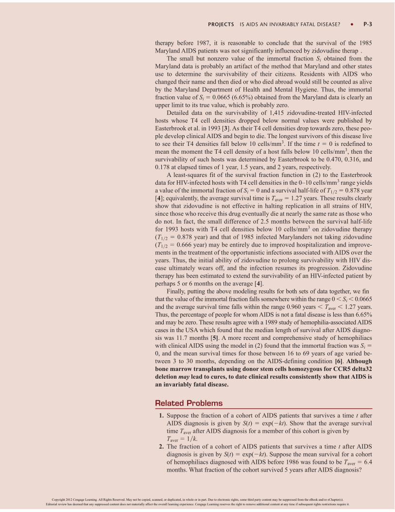
Related Problems1. Suppose the fraction of a cohort of AIDS patients that survives a time t after
AIDS diagnosis is given by S(t) exp(kt). Show that the average survivaltime Taver after AIDS diagnosis for a member of this cohort is given byTaver 1k.
2. The fraction of a cohort of AIDS patients that survives a time t after AIDSdiagnosis is given by S(t) exp(kt). Suppose the mean survival for a cohortof hemophiliacs diagnosed with AIDS before 1986 was found to be Taver 6.4months. What fraction of the cohort survived 5 years after AIDS diagnosis?
PROJECTS IS AIDS AN INVARIABLY FATAL DISEASE? P-3
Copyright 2012 Cengage Learning. All Rights Reserved. May not be copied, scanned, or duplicated, in whole or in part. Due to electronic rights, some third party content may be suppressed from the eBook and/or eChapter(s).
Editorial review has deemed that any suppressed content does not materially affect the overall learning experience. Cengage Learning reserves the right to remove additional content at any time if subsequent rights restrictions require it.

3. The fraction of a cohort of AIDS patients that survives a time t after AIDS diag-nosis is given by S(t) exp(kt). The time it takes for S(t) to reach the value of0.5 is defined as the survival half-life and denoted by T12.(a) Show that S(t) can be written in the form .(b) Show that T12 Taver ln(2), where Taver is the average survival time define
in problem (1). Thus, it is always true that T12 Taver.4. About 10% of lung cancer patients are cured of the disease, i.e., they survive
5 years after diagnosis with no evidence that the cancer has returned. Only 14%of lung cancer patients survive 5 years after diagnosis. Assume that the fractionof incurable lung cancer patients that survives a time t after diagnosis is givenby exp(kt). Find an expression for the fraction S(t) of lung cancer patients thatsurvive a time t after being diagnosed with the disease. Be sure to determine thevalues of all of the constants in your answer. What fraction of lung cancer patientssurvives two years with the disease?
References1. Kramer, Ivan. What triggers transient AIDS in the acute phase of HIV infection
and chronic AIDS at the end of the incubation period? Computational andMathematical Methods in Medicine, Vol. 8, No. 2, June 2007: 125–151.
2. Kramer, Ivan. Is AIDS an invariable fatal disease?: A model analysis of AIDSsurvival curves. Mathematical and Computer Modelling 15, no. 9, 1991: 1–19.
3. Easterbrook, Philippa J., Emani Javad, Moyle, Graham, Gazzard, Brian G.Progressive CD4 cell depletion and death in zidovudine-treated patients. JAIDS,Aug. 6, 1993, No. 8: 927–929.
4. Kramer, Ivan. The impact of zidovudine (AZT) therapy on the survivability ofthose with progressive HIV infection. Mathematical and Computer Modelling,Vol. 23, No. 3, Feb. 1996: 1–14.
5. Stehr-Green, J. K., Holman, R. C., Mahoney, M. A. Survival analysis of hemophilia-associated AIDS cases in the US. Am J Public Health, Jul. 1989, 79(7): 832–835.
6. Gail, Mitchel H., Tan, Wai-Yuan, Pee, David, Goedert, James J. Survival afterAIDS diagnosis in a cohort of hemophilia patients. JAIDS, Aug. 15, 1997,Vol. 15, No. 5: 363–369.
ABOUT THE AUTHOR Ivan Kramer earned a BS in Physics and Mathematics from The City College ofNew York in 1961 and a PhD from the University of California at Berkeley in theo-retical particle physics in 1967. He is currently associate professor of physics at theUniversity of Maryland, Baltimore County. Dr. Kramer was Project Director forAIDS/HIV Case Projections for Maryland, for which he received a grant from theAIDS Administration of the Maryland Department of Health and Hygiene in 1990.In addition to his many published articles on HIV infection and AIDS, his currentresearch interests include mutation models of cancers, Alzheimers disease, andschizophrenia.
S(t) 2t>T1>2
P-4 PROJECTS IS AIDS AN INVARIABLY FATAL DISEASE?
Cou
rtes
y of
Iva
n K
ram
er
Copyright 2012 Cengage Learning. All Rights Reserved. May not be copied, scanned, or duplicated, in whole or in part. Due to electronic rights, some third party content may be suppressed from the eBook and/or eChapter(s).
Editorial review has deemed that any suppressed content does not materially affect the overall learning experience. Cengage Learning reserves the right to remove additional content at any time if subsequent rights restrictions require it.

The Allee Effectby Jo Gascoigne
The top five most famous Belgians apparently include a cyclist, a punk singer, the in-ventor of the saxophone, the creator of Tintin, and Audrey Hepburn. Pierre FrançoisVerhulst is not on the list, although he should be. He had a fairly short life, dying atthe age of 45, but did manage to include some excitement—he was deported fromRome for trying to persuade the Pope that the Papal States needed a written constitu-tion. Perhaps the Pope knew better even then than to take lectures in good gover-nance from a Belgian. . . .
Aside from this episode, Pierre Verhulst (1804–1849) was a mathematician whoconcerned himself, among other things, with the dynamics of natural populations—fish, rabbits, buttercups, bacteria, or whatever. (I am prejudiced in favour of fish, sowe will be thinking fish from now on.) Theorizing on the growth of natural popula-tions had up to this point been relatively limited, although scientists had reached theobvious conclusion that the growth rate of a population (dNdt, where N(t) is thepopulation size at time t) depended on (i) the birth rate b and (ii) the mortality rate m,both of which would vary in direct proportion to the size of the population N:
(1)
After combining b and m into one parameter r, called the intrinsic rate of naturalincrease—or more usually by biologists without the time to get their tongues aroundthat, just r—equation (1) becomes
(2)
This model of population growth has a problem, which should be clear to you—ifnot, plot dNdt for increasing values of N. It is a straightforward exponential growthcurve, suggesting that we will all eventually be drowning in fish. Clearly, somethingeventually has to step in and slow down dNdt. Pierre Verhulst’s insight was that thissomething was the capacity of the environment, in other words,
How many fish can an ecosystem actually support?
He formulated a differential equation for the population N(t) that included bothr and the carrying capacity K:
(3)
Equation (3) is called the logistic equation, and it forms to this day the basis of muchof the modern science of population dynamics. Hopefully, it is clear that the term(1 NK), which is Verhulst’s contribution to equation (2), is (1 NK) 1 whenN 0, leading to exponential growth, and (1 NK) : 0 as N : K, hence it causesthe growth curve of N(t) to approach the horizontal asymptote N(t) K. Thus the sizeof the population cannot exceed the carrying capacity of the environment.
dN
dt rN1
N
K, r 0.
dN
dt rN.
dN
dt bN mN.
P-5
Project for Section 3.2
Dr Jo with Queenie; Queenie is on the left
Cou
rtes
y of
Jo
Gas
oign
e
Copyright 2012 Cengage Learning. All Rights Reserved. May not be copied, scanned, or duplicated, in whole or in part. Due to electronic rights, some third party content may be suppressed from the eBook and/or eChapter(s).
Editorial review has deemed that any suppressed content does not materially affect the overall learning experience. Cengage Learning reserves the right to remove additional content at any time if subsequent rights restrictions require it.

P-6 PROJECTS THE ALLEE EFFECT
The logistic equation (3) gives the overall growth rate of the population, but theecology is easier to conceptualize if we consider per capita growth rate—that is, thegrowth rate of the population per the number of individuals in the population—somemeasure of how “well” each individual in the population is doing. To get per capitagrowth rate, we just divide each side of equation (3) by N:
This second version of (3) immediately shows (or plot it) that this relationship is a
straight line with a maximum value of (assuming that negative popu-
lation sizes are not relevant) and dNdt 0 at N K.
Er, hang on a minute . . . “a maximum value of ” Each shark in
the population does best when there are . . . zero sharks? Here is clearly a flaw in thelogistic model. (Note that it is now a model—when it just presents a relationship be-tween two variables dNdt and N, it is just an equation. When we use this equationto try and analyze how populations might work, it becomes a model.)
The assumption behind the logistic model is that as population size decreases, indi-viduals do better (as measured by the per capita population growth rate). This assump-tion to some extent underlies all our ideas about sustainable management of naturalresources—a fish population cannot be fished indefinitely unless we assume that whena population is reduced in size, it has the ability to grow back to where it was before.
This assumption is more or less reasonable for populations, like many fish pop-ulations subject to commercial fisheries, which are maintained at 50% or even 20%of K. But for very depleted or endangered populations, the idea that individuals keepdoing better as the population gets smaller is a risky one. The Grand Banks popula-tion of cod, which was fished down to 1% or perhaps even 0.1% of K, has been pro-tected since the early 1990s, and has yet to show convincing signs of recovery.
Warder Clyde Allee (1885–1955) was an American ecologist at the Universityof Chicago in the early 20th century, who experimented on goldfish, brittlestars, floubeetles, and, in fact, almost anything unlucky enough to cross his path. Allee showedthat, in fact, individuals in a population can do worse when the population becomesvery small or very sparse.* There are numerous ecological reasons why this mightbe—for example, they may not find a suitable mate or may need large groups to finfood or express social behavior, or in the case of goldfish they may alter the waterchemistry in their favour. As a result of Allee’s work, a population where the percapita growth rate declines at low population size is said to show an Allee effect. Thejury is still out on whether Grand Banks cod are suffering from an Allee effect, butthere are some possible mechanisms—females may not be able to find a mate, or amate of the right size, or maybe the adult cod used to eat the fish that eat the juvenilecod. On the other hand, there is nothing that an adult cod likes more than a snack ofbaby cod—they are not fish with very picky eating habits—so these arguments maynot stack up. For the moment we know very little except that there are still no cod.
Allee effects can be modelled in many ways. One of the simplest mathematicalmodels, a variation of the logistic equation, is:
(4)
where A is called the Allee threshold. The value N (t) A is the population size belowwhich the population growth rate becomes negative due to an Allee effect—situated at
dN
dt rN1
N
KN
A 1.
1
N dN
dt at N 0?!
1
N dN
dt at N 0
1
N dN
dt r1
N
K r r
KN.
*Population size and population density are mathematically interchangeable, assuming a fixed area iwhich the population lives (although they may not necessarily be interchangeable for the individuals inquestion).
Copyright 2012 Cengage Learning. All Rights Reserved. May not be copied, scanned, or duplicated, in whole or in part. Due to electronic rights, some third party content may be suppressed from the eBook and/or eChapter(s).
Editorial review has deemed that any suppressed content does not materially affect the overall learning experience. Cengage Learning reserves the right to remove additional content at any time if subsequent rights restrictions require it.

PROJECTS THE ALLEE EFFECT P-7
a value of N somewhere between N 0 and N K, that is, 0 A K, depending onthe species (but for most species a good bit closer to 0 than K, luckily).
Equation (4) is not as straightforward to solve for N(t) as (3), but we don’t needto solve it to gain some insights into its dynamics. If you work through Problems 2and 3, you will see that the consequences of equation (4) can be disastrous for endan-gered populations.
Related Problems1. (a) The logistic equation (3) can be solved explicitly for N(t) using the technique
of partial fractions. Do this, and plot N(t) as a function of t for 0 t 10.Appropriate values for r, K, and N(0) are r 1, K 1, N(0) 0.01 (fish percubic metre of seawater, say). The graph of N(t) is called a sigmoid growthcurve.
(b) The value of r can tell us a lot about the ecology of a species—sardines,where females mature in less than one year and have millions of eggs, havea high r, while sharks, where females bear a few live young each year, havea low r. Play with r and see how it affects the shape of the curve. Question:If a marine protected area is put in place to stop overfishing, which specieswill recover quickest—sardines or sharks?
2. Find the population equilibria for the model in (4). [Hint: The population is atequilibrium when dNdt 0, that is, the population is neither growing norshrinking. You should find three values of N for which the population is at equi-librium.]
3. Population equilibria can be stable or unstable. If, when a population deviates abit from the equilibrium value (as populations inevitably do), it tends to return toit, this is a stable equilibrium; if, however, when the population deviates fromthe equilibrium it tends to diverge from it ever further, this is an unstable equi-librium. Think of a ball in the pocket of a snooker table versus a ball balanced ona snooker cue. Unstable equilibria are a feature of Allee effect models such as(4). Use a phase portrait of the autonomous equation (4) to determine whetherthe nonzero equilibria that you found in Problem 2 are stable or unstable. [Hint:See Section 2.1 of the text.]
4. Discuss the consequences of the result above for a population N(t) fluctuatinclose to the Allee threshold A.
References1. Courchamp, F., Berec L., and Gascoigne, J. 2008. Allee Effects in Ecology and
Conservation. Oxford University Press.2. Hastings, A. 1997. Population Biology—Concepts and Models. Springer-Verlag,
New York.
ABOUT THE AUTHOR After a degree in Zoology, Jo Gascoigne thought her first job, on conservation inEast Africa, would be about lions and elephants—but it turned out to be about fishDespite the initial crushing disappointment, she ended up loving them—so much, infact, that she went on to complete a PhD in marine conservation biology at theCollege of William and Mary, in Williamsburg, Virginia, where she studied lobster andCaribbean conch, and also spent 10 days living underwater in the Aquarius habitat inFlorida. After graduating, she returned to her native Britain and studied the mathemat-ics of mussel beds at Bangor University in Wales, before becoming an independentconsultant on fisheries management. She now works to promote environmentally sus-tainable fisheries. When you buy seafood, make good choices and help the sea!
Copper sharks and bronze whaler sharksfeeding on a bait ball of sardines off theeast coast of South Africa
Cou
rtes
y of
Jo
Gas
coig
neD
oug
Per
rine
/Get
ty I
mag
es
Copyright 2012 Cengage Learning. All Rights Reserved. May not be copied, scanned, or duplicated, in whole or in part. Due to electronic rights, some third party content may be suppressed from the eBook and/or eChapter(s).
Editorial review has deemed that any suppressed content does not materially affect the overall learning experience. Cengage Learning reserves the right to remove additional content at any time if subsequent rights restrictions require it.

P-8 PROJECTS THE ALLEE EFFECT
Project for Section 3.3
Wolf Population Dynamicsby C. J. Knickerbocker
Early in 1995, after much controversy, public debate, and a 70-year absence, graywolves were re introduced into Yellowstone National Park and Central Idaho. Duringthis 70-year absence, significant changes were recorded in the populations of otherpredator and prey animals residing in the park. For instance, the elk and coyote pop-ulations had risen in the absence of influence from the larger gray wolf. With thereintroduction of the wolf in 1995, we anticipated changes in both the predator andprey animal populations in the Yellowstone Park ecosystem as the success of thewolf population is dependent upon how it influences and is influenced by the otherspecies in the ecosystem.
For this study, we will examine how the elk (prey) population has been influenced by the wolves (predator). Recent studies have shown that the elk populationhas been negatively impacted by the reintroduction of the wolves. The elk populationfell from approximately 18,000 in 1995 to approximately 7,000 in 2009. This articleasks the question of whether the wolves could have such an effect and, if so, couldthe elk population disappear?
Let’s begin with a more detailed look at the changes in the elk population inde-pendent of the wolves. In the 10 years prior to the introduction of wolves, from 1985to 1995, one study suggested that the elk population increased by 40% from 13,000in 1985 to 18,000 in 1995. Using the simplest differential equation model for popu-lation dynamics, we can determine the growth rate for elks (represented by the vari-able r) prior to the reintroduction of the wolves.
(1)
In this equation, E(t) represents the elk population (in thousands) where t is measuredin years since 1985. The solution, which is left as an exercise for the reader, finds thecombined birth/death growth rate r to be approximately 0.0325 yielding:
In 1995, 21 wolves were initially released, and their numbers have risen. In2007, biologists estimated the number of wolves to be approximately 171.
To study the interaction between the elk and wolf populations, let’s consider thefollowing predator-prey model for the interaction between the elk and wolf withinthe Yellowstone ecosystem:
(2)
where E(t) is the elk population and W(t) is the wolf population. All populations aremeasured in thousands of animals. The variable t represents time measured in yearsfrom 1995. So, from the initial conditions, we have 18,000 elk and 21 wolves in theyear 1995. The reader will notice that we estimated the growth rate for the elk to bethe same as that estimated above r 0.0325.
E(0) 18.0, W(0) 0.021
dW
dt 0.6W 0.05EW
dE
dt 0.0325E 0.8EW
E(t) 13.0 e0.0325t
E(10) 18.0E(0) 13.0,dE
dt rE,
A gray wolf in the wild
P-8
Dam
ien
Ric
hard
/Shu
tter
stoc
k.co
m
Copyright 2012 Cengage Learning. All Rights Reserved. May not be copied, scanned, or duplicated, in whole or in part. Due to electronic rights, some third party content may be suppressed from the eBook and/or eChapter(s).
Editorial review has deemed that any suppressed content does not materially affect the overall learning experience. Cengage Learning reserves the right to remove additional content at any time if subsequent rights restrictions require it.

Before we attempt to solve the model (2), a qualitative analysis of the systemcan yield a number of interesting properties of the solutions. The first equationshows that the growth rate of the elk is positively impacted by the size ofthe herd (0.0325E). This can be interpreted as the probability of breeding in-creases with the number of elk. On the other hand the nonlinear term (0.8EW) hasa negative impact on the growth rate of the elk since it measures the interactionbetween predator and prey. The second equation shows that the wolf population has a negative effect on its own growth which canbe interpreted as more wolves create more competition for food. But, the interac-tion between the elk and wolves (0.05EW) has a positive impact since the wolvesare finding more food.
Since an analytical solution cannot be found to the initial-value problem (2), weneed to rely on technology to find approximate solutions. For example, below is a setof instructions for finding a numerical solution of the initial-value problem using thecomputer algebra system MAPLE.
e1 := diff(e(t),t)- 0.0325 * e(t) + 0.8 * e(t)*w(t) :e2 := diff(w(t),t)+ 0.6 * w(t) - 0.05 * e(t)*w(t) :sys := e1,e2 :ic := e(0)=18.0,w(0)=0.021 :ivp := sys union ic :H:= dsolve(ivp,e(t),w(t),numeric) :
The graphs in Figures 1 and 2 show the populations for both species between 1995and 2009. As predicted by numerous studies, the reintroduction of wolves intoYellowstone had led to a decline in the elk population. In this model, we see the popula-tion decline from 18,000 in 1995 to approximately 7,000 in 2009. In contrast, the wolfpopulation rose from an initial count of 21 in 1995 to a high of approximately 180 in2004.
dW>dt 0.6W 0.05EW
(dE>dt)
The alert reader will note that the model also shows a decline in the wolf popu-lation after 2004. How might we interpret this? With the decline in the elk populationover the first 10 years, there was less food for the wolves and therefore their popula-tion begins to decline.
Figure 3 below shows the long-term behavior of both populations. The interpre-tation of this graph is left as an exercise for the reader.
Information on the reintroduction of wolves into Yellowstone Park and centralIdaho can be found on the Internet. For example, read the U.S. Fish and WildlifeService news release of November 23, 1994, on the release of wolves intoYellowstone National Park.
20000
18000
16000
14000
12000
10000
8000
6000
4000
2000
1995 1997 1999 2001
Year
Elk
pop
ulat
ion
2003 2005 2007 20090
200
180
160
140
120
100
80
60
40
20
1995 1997 1999 2001Year
Wol
f po
pula
tion
2003 2005 2007 20090
PROJECTS WOLF POPULATION DYNAMICS P-9
FIGURE 1 Elk population FIGURE 2 Wolf population
Copyright 2012 Cengage Learning. All Rights Reserved. May not be copied, scanned, or duplicated, in whole or in part. Due to electronic rights, some third party content may be suppressed from the eBook and/or eChapter(s).
Editorial review has deemed that any suppressed content does not materially affect the overall learning experience. Cengage Learning reserves the right to remove additional content at any time if subsequent rights restrictions require it.

P-10 PROJECTS WOLF POPULATION DYNAMICS
Related Problems1. Solve the pre-wolf initial-value problem (1) by first solving the differential
equation and applying the initial condition. Then apply the terminal condition tofind the growth rate
2. Biologists have debated whether the decrease in the elk from 18,000 in 1995 to7,000 in 2009 is due to the reintroduction of wolves. What other factors mightaccount for the decrease in the elk population?
3. Consider the long-term changes in the elk and wolf populations. Are these cyclicchanges reasonable? Why is there a lag between the time when the elk begins todecline and the wolf population begins to decline? Are the minimum values forthe wolf population realistic? Plot the elk population versus the wolf populationand interpret the results.
4. What does the initial-value problem (1) tell us about the growth of the elk pop-ulation without the influence of the wolves? Find a similar model for the intro-duction of rabbits into Australia in 1859 and the impact of introducing a preypopulation into an environment without a natural predator population.
20000
18000
16000
14000
12000
10000
8000
6000
4000
2000
0
200
180
160
140
120
100
80
60
40
20
01990 2000 2010 2020 2030 2040 2050 2060 2070 2080
Year
Elk
and
Wol
f P
opul
atio
ns
Elk
Wolf
ABOUT THE AUTHOR C. J. KnickerbockerProfessor of Mathematics and Computer Science (retired)St. Lawrence UniversityPrincipal Research EngineerSensis Corporation
C. J. Knickerbocker received his PhD in mathematics from Clarkson University in1984. Until 2008 he was a professor of mathematics and computer science atSt. Lawrence University, where he authored numerous articles in a variety of topics,including nonlinear partial differential equations, graph theory, applied physics, andpsychology. He has also served as a consultant for publishers, software companies,and government agencies. Currently, Dr. Knickerbocker is a principal research engi-neer for the Sensis Corporation, where he studies airport safety and efficienc .
FIGURE 3 Long-term behavior of the populations
Cou
rtes
y of
C. J
. Kni
cker
bock
er
Copyright 2012 Cengage Learning. All Rights Reserved. May not be copied, scanned, or duplicated, in whole or in part. Due to electronic rights, some third party content may be suppressed from the eBook and/or eChapter(s).
Editorial review has deemed that any suppressed content does not materially affect the overall learning experience. Cengage Learning reserves the right to remove additional content at any time if subsequent rights restrictions require it.

Bungee Jumpingby Kevin Cooper
Suppose that you have no sense. Suppose that you are standing on a bridge above theMalad River canyon. Suppose that you plan to jump off that bridge. You have no sui-cide wish. Instead, you plan to attach a bungee cord to your feet, to dive gracefullyinto the void, and to be pulled back gently by the cord before you hit the river that is174 feet below. You have brought several different cords with which to affix yourfeet, including several standard bungee cords, a climbing rope, and a steel cable. Youneed to choose the stiffness and length of the cord so as to avoid the unpleasantnessassociated with an unexpected water landing. You are undaunted by this task, becauseyou know math!
Each of the cords you have brought will be tied off so as to be 100 feet longwhen hanging from the bridge. Call the position at the bottom of the cord 0, andmeasure the position of your feet below that “natural length” as x(t), where x increasesas you go down and is a function of time t. See Figure 1. Then, at the time youjump, x(0) = -100, while if your six-foot frame hits the water head first, at that timex(t) = 174 - 100 - 6 = 68. Notice that distance increases as you fall, and so yourvelocity is positive as you fall and negative when you bounce back up. Note alsothat you plan to dive so your head will be six feet below the end of the chord whenit stops you.
You know that the acceleration due to gravity is a constant, called g, so that theforce pulling downwards on your body is mg. You know that when you leap from thebridge, air resistance will increase proportionally to your speed, providing a force inthe opposite direction to your motion of about bv, where b is a constant and v is yourvelocity. Finally, you know that Hooke’s law describing the action of springs saysthat the bungee cord will eventually exert a force on you proportional to its distancepast its natural length. Thus, you know that the force of the cord pulling you backfrom destruction may be expressed as
The number k is called the spring constant, and it is where the stiffness of the cordyou use influences the equation. For example, if you used the steel cable, then kwould be very large, giving a tremendous stopping force very suddenly as you passedthe natural length of the cable. This could lead to discomfort, injury, or even aDarwin award. You want to choose the cord with a k value large enough to stop youabove or just touching the water, but not too suddenly. Consequently, you are inter-ested in finding the distance you fall below the natural length of the cord as a func-tion of the spring constant. To do that, you must solve the differential equation thatwe have derived in words above: The force mx on your body is given by
mx mg + b(x) - bx.
Here mg is your weight, 160 lb., and x is the rate of change of your position belowthe equilibrium with respect to time; i.e., your velocity. The constant b for air resis-tance depends on a number of things, including whether you wear your skin-tightpink spandex or your skater shorts and XXL T-shirt, but you know that the valuetoday is about 1.0.
b(x) 0
kx
x 0
x 0
P-11
Project for Section 5.1
100 ft
Bridge
Bungee
174 ft
x = −100
x = 0
x = 74
Water
FIGURE 1 The bungee setup
Bungee jumping from a bridge
Sea
n N
el/S
hutt
erst
ock.
com
Copyright 2012 Cengage Learning. All Rights Reserved. May not be copied, scanned, or duplicated, in whole or in part. Due to electronic rights, some third party content may be suppressed from the eBook and/or eChapter(s).
Editorial review has deemed that any suppressed content does not materially affect the overall learning experience. Cengage Learning reserves the right to remove additional content at any time if subsequent rights restrictions require it.

This is a nonlinear differential equation, but inside it are two linear differentialequations, struggling to get out. We will work with such equations more extensivelyin later chapters, but we already know how to solve such equations from our pastexperience. When x 0, the equation is mx = mg - bx, while after you pass thenatural length of the cord it is mx = mg - kx - bx. We will solve these separately,and then piece the solutions together when x(t) = 0.
In Problem 1 you find an expression for your position t seconds after you step offthe bridge, before the bungee cord starts to pull you back. Notice that it does notdepend on the value for k, because the bungee cord is just falling with you when youare above x(t) = 0. When you pass the natural length of the bungee cord, it does startto pull back, so the differential equation changes. Let t1 denote the first time for whichx(t1) = 0, and let v1 denote your speed at that time. We can thus describe the motionfor x(t) 0 using the problem x = g - kx - bx, x(t1) = 0, x(t1) = v1. An illustrationof a solution to this problem in phase space can be seen in Figure 2.
This will yield an expression for your position as the cord is pulling on you. Allwe have to do is to find out the time t2 when you stop going down. When you stopgoing down, your velocity is zero, i.e., x(t2) = 0.
As you can see, knowing a little bit of math is a dangerous thing. We remindyou that the assumption that the drag due to air resistance is linear applies only forlow speeds. By the time you swoop past the natural length of the cord, that approx-imation is only wishful thinking, so your actual mileage may vary. Moreover,springs behave nonlinearly in large oscillations, so Hooke’s law is only an approx-imation. Do not trust your life to an approximation made by a man who has beendead for 200 years. Leave bungee jumping to the professionals.
Related Problems1. Solve the equation mx + bx = mg for x(t), given that you step off the bridge—no
jumping, no diving! Stepping off means x(0) = -100, x(0) = 0. You may usemg = 160, b = 1, and g = 32.
2. Use the solution from Problem 1 to compute the length of time t1 that you freefall(the time it takes to go the natural length of the cord: 100 feet).
3. Compute the derivative of the solution you found in Problem 1 and evaluate it atthe time you found in Problem 2. Call the result v1. You have found your down-ward speed when you pass the point where the cord starts to pull.
4. Solve the initial-value problem
For now, you may use the value k = 14, but eventually you will need to replacethat with the actual values for the cords you brought. The solution x(t) repre-sents the position of your feet below the natural length of the cord after it startsto pull back.
5. Compute the derivative of the expression you found in Problem 4 and solve forthe value of t where it is zero. This time is t2. Be careful that the time you computeis greater than t1—there are several times when your motion stops at the top andbottom of your bounces! After you find t2, substitute it back into the solution youfound in Problem 4 to find your lowest position
6. You have brought a soft bungee cord with k = 8.5, a stiffer cord with k = 10.7, anda climbing rope for which k = 16.4. Which, if any, of these may you use safelyunder the conditions given?
7. You have a bungee cord for which you have not determined the spring constant.To do so, you suspend a weight of 10 lb. from the end of the 100-foot cord, caus-ing the cord to stretch 1.2 feet. What is the k value for this cord? You may neglectthe mass of the cord itself.
x(t1) v1.x(t1) 0, mx bx kx mg,
FIGURE 2 An example plot of x(t)against x(t) for a bungee jump
60
40
20
20 40
_20
_20 0_40_60_80_100
_40
x(t)
x'(t)
P-12 PROJECTS BUNGEE JUMPING
Copyright 2012 Cengage Learning. All Rights Reserved. May not be copied, scanned, or duplicated, in whole or in part. Due to electronic rights, some third party content may be suppressed from the eBook and/or eChapter(s).
Editorial review has deemed that any suppressed content does not materially affect the overall learning experience. Cengage Learning reserves the right to remove additional content at any time if subsequent rights restrictions require it.

PROJECTS BUNGEE JUMPING P-13
ABOUT THE AUTHOR Kevin Cooper, PhD, Colorado State University, is the Computing Coordinator forMathematics at Washington State University, Pullman, Washington. His main inter-est is numerical analysis, and he has written papers and one textbook in that area. Dr.Cooper also devotes considerable time to creating mathematical software compo-nents, such as DynaSys, a program to analyze dynamical systems numerically.
Cou
rtes
y of
Kev
in C
oope
r
Copyright 2012 Cengage Learning. All Rights Reserved. May not be copied, scanned, or duplicated, in whole or in part. Due to electronic rights, some third party content may be suppressed from the eBook and/or eChapter(s).
Editorial review has deemed that any suppressed content does not materially affect the overall learning experience. Cengage Learning reserves the right to remove additional content at any time if subsequent rights restrictions require it.

The Collapse of the TacomaNarrows Suspension Bridgeby Gilbert N. Lewis
In the summer of 1940, the Tacoma Narrows Suspension Bridge in the State ofWashington was completed and opened to traffic.Almost immediately, observers no-ticed that the wind blowing across the roadway would sometimes set up large verti-cal vibrations in the roadbed. The bridge became a tourist attraction as people cameto watch, and perhaps ride, the undulating bridge. Finally, on November 7, 1940, dur-ing a powerful storm, the oscillations increased beyond any previously observed, andthe bridge was evacuated. Soon, the vertical oscillations became rotational, as ob-served by looking down the roadway. The entire span was eventually shaken apart bythe large vibrations, and the bridge collapsed. Figure 1 shows a picture of the bridgeduring the collapse. See [1] and [2] for interesting and sometimes humorous anec-dotes associated with the bridge. Or, do an Internet search with the key words“Tacoma Bridge Disaster” in order to find and view some interesting videos of thecollapse of the bridge.
The noted engineer von Karman was asked to determine the cause of the col-lapse. He and his coauthors [3] claimed that the wind blowing perpendicularly acrossthe roadway separated into vortices (wind swirls) alternately above and below theroadbed, thereby setting up a periodic, vertical force acting on the bridge. It was thisforce that caused the oscillations. Others further hypothesized that the frequency ofthis forcing function exactly matched the natural frequency of the bridge, thus lead-ing to resonance, large oscillations, and destruction. For almost fifty years, resonancewas blamed as the cause of the collapse of the bridge, although the von Karmangroup denied this, stating that “it is very improbable that resonance with alternatingvortices plays an important role in the oscillations of suspension bridges” [3].
As we can see from equation (31) in Section 5.1.3, resonance is a linear phe-nomenon. In addition, for resonance to occur, there must be an exact match betweenthe frequency of the forcing function and the natural frequency of the bridge.Furthermore, there must be absolutely no damping in the system. It should not besurprising, then, that resonance was not the culprit in the collapse.
If resonance did not cause the collapse of the bridge, what did? Recent researchprovides an alternative explanation for the collapse of the Tacoma Narrows Bridge.Lazer and McKenna [4] contend that nonlinear effects, and not linear resonance,were the main factors leading to the large oscillations of the bridge (see [5] for a goodreview article). The theory involves partial differential equations. However, a simpli-fied model leading to a nonlinear ordinary differential equation can be constructed.
The development of the model below is not exactly the same as that of Lazer andMcKenna, but it results in a similar differential equation. This example shows an-other way that amplitudes of oscillation can increase.
Consider a single vertical cable of the suspension bridge. We assume that it actslike a spring, but with different characteristics in tension and compression, and withno damping. When stretched, the cable acts like a spring with Hooke’s constant, b,while, when compressed, it acts like a spring with a different Hooke’s constant, a. Weassume that the cable in compression exerts a smaller force on the roadway thanwhen stretched the same distance, so that 0 a b. Let the vertical deflectio(positive direction downward) of the slice of the roadbed attached to this cable be
The rebuilt Tacoma Narrows bridge (1950)and new parallel bridge (2009)
Collapse of the Tacoma Narrows Bridge
Project for Section 5.3
AP
Pho
to
P-14
Sir
Arm
stro
ng/S
hutt
erst
ock.
com
Copyright 2012 Cengage Learning. All Rights Reserved. May not be copied, scanned, or duplicated, in whole or in part. Due to electronic rights, some third party content may be suppressed from the eBook and/or eChapter(s).
Editorial review has deemed that any suppressed content does not materially affect the overall learning experience. Cengage Learning reserves the right to remove additional content at any time if subsequent rights restrictions require it.

denoted by y(t), where t represents time, and y 0 represents the equilibrium posi-tion of the road. As the roadbed oscillates under the influence of an applied verticalforce (due to the von Karman vortices), the cable provides an upward restoring forceequal to by when y 0 and a downward restoring force equal to ay when y 0. Thischange in the Hooke’s Law constant at y 0 provides the nonlinearity to the differ-ential equation. We are thus led to consider the differential equation derived fromNewton’s second law of motion
my f(y) g(t),
where f(y) is the nonlinear function given by
g(t) is the applied force, and m is the mass of the section of the roadway. Note thatthe differential equation is linear on any interval on which y does not change sign.
Now, let us see what a typical solution of this problem would look like. We willassume that m 1 kg, b 4 N/m, a 1N/m, and g(t) sin(4t) N. Note that the fre-quency of the forcing function is larger than the natural frequencies of the cable inboth tension and compression, so that we do not expect resonance to occur. We alsoassign the following initial values to y: y(0) 0, y(0) 0.01, so that the roadbedstarts in the equilibrium position with a small downward velocity.
Because of the downward initial velocity and the positive applied force, y(t) willinitially increase and become positive. Therefore, we first solve this initial-valueproblem
y 4y sin(4t), y(0) 0, y(0) 0.01. (1)
The solution of the equation in (1), according to Theorem 4.1.6, is the sum of thecomplementary solution, yc(t), and the particular solution, yp(t). It is easy to seethat yc(t) c1cos(2t) c2sin(2t) (equation (9), Section 4.3), and yp(t) (Table 4.4.1, Section 4.4). Thus,
y(t) c1cos(2t) c2 sin(2t) . (2)
The initial conditions give
y(0) 0 c1,
y(0) 0.01 2c2 ,
so that c2 (0.01 )2. Therefore, (2) becomes
(3)
We note that the first positive value of t for which y(t) is again equal to zero is .At that point, Therefore, equation (3) holds on [0, ].
After becomes negative, so we must now solve the new problem
(4)
Proceeding as above, the solution of (4) is
(5) cos t0.01
2
5 4
15sin t cos(2t).
y(t) 0.01 2
5cos t 1
15sin(4t)
y y sin(4t), yp2 0, yp2 0.01 2
3.
t p
2 , yp>2y(p2) (0.01 2
3).t p
2
sin(2t)1
20.01 1
3 1
6cos(2t).
y(t) 1
20.01 1
3sin(2t) 1
12sin(4t)
13
1
3
1
12sin(4t)
112 sin(4t)
f(y) by if y 0ay if y 0,
PROJECTS THE COLLAPSE OF THE TACOMA NARROWS SUSPENSION BRIDGE P-15
Copyright 2012 Cengage Learning. All Rights Reserved. May not be copied, scanned, or duplicated, in whole or in part. Due to electronic rights, some third party content may be suppressed from the eBook and/or eChapter(s).
Editorial review has deemed that any suppressed content does not materially affect the overall learning experience. Cengage Learning reserves the right to remove additional content at any time if subsequent rights restrictions require it.

P-16 PROJECTS THE COLLAPSE OF THE TACOMA NARROWS SUSPENSION BRIDGE
The next positive value of t after at which y(t) 0 is at which pointso that equation (5) holds on .
At this point, the solution has gone through one cycle in the time interval During this cycle, the section of the roadway started at the equilibrium with positivevelocity, became positive, came back to the equilibrium position with negative ve-locity, became negative, and finally returned to the equilibrium position with positivevelocity. This pattern continues indefinitel , with each cycle covering time units.The solution for the next cycle is
(6)
It is instructive to note that the velocity at the beginning of the second cycle is(0.01 ), while at the beginning of the third cycle it is (0.01 ). In fact, thevelocity at the beginning of each cycle is greater than at the beginning of the pre-vious cycle. It is not surprising then that the amplitude of oscillations will increaseover time, since the amplitude of (one term in) the solution during any one cycle isdirectly related to the velocity at the beginning of the cycle. See Figure 2 for agraph of the deflection function on the interval [0, 3p]. Note that the maximumdeflection on [3p2, 2p] is larger than the maximum deflection on [0, p2], whilethe maximum deflection on [2p, 3p] is larger than the maximum deflection on[p2, 3p2].
It must be remembered that the model presented here is a very simplified one-dimensional model that cannot take into account all of the intricate interactions ofreal bridges. The reader is referred to the account by Lazer and McKenna [4] for amore complete model. More recently, McKenna [6] has refined that model to providea different viewpoint of the torsional oscillations observed in the Tacoma Bridge.
Research on the behavior of bridges under forces continues. It is likely thatthe models will be refined over time, and new insights will be gained from theresearch. However, it should be clear at this point that the large oscillations caus-ing the destruction of the Tacoma Narrows Suspension Bridge were not the resultof resonance.
215
415 2
15
y(t) sin t0.01 8
15 4
15cos t cos(2t) on [2p, 3p].
y(t) sin(2t)1
20.01 7
15 1
6cos(2t) on [3p>2, 2p],
3p2
[0, 3p2 ].[p>2, 3p>2]y(3p
2 ) 0.01 215,
t 3p2 ,t p
2
0.2
y
t0.02 4 6 8
−0.2
−0.4
−0.6
FIGURE 2 Graph of deflection function y(t)
Related Problems1. Solve the following problems and plot the solutions for 0 t 6p. Note that reso-
nance occurs in the first problem but not in the second
(a)(b) y y cos(2t), y(0) 0, y(0) 0.
y y cos t, y(0) 0, y(0) 0.
Copyright 2012 Cengage Learning. All Rights Reserved. May not be copied, scanned, or duplicated, in whole or in part. Due to electronic rights, some third party content may be suppressed from the eBook and/or eChapter(s).
Editorial review has deemed that any suppressed content does not materially affect the overall learning experience. Cengage Learning reserves the right to remove additional content at any time if subsequent rights restrictions require it.

PROJECTS THE COLLAPSE OF THE TACOMA NARROWS SUSPENSION BRIDGE P-17
2. Solve the initial-value problem where
and (a) b 1, a 4, (Compare your answer with the example in this project.)(b) b 64, a 4,(c) b 36, a 25.
Note that, in part (a), the condition b a of the text is not satisfied. Plot the solu-tions. What happens in each case as t increases? What would happen in each caseif the second initial condition were replaced with y(0) 0.01? Can you make anyconclusions similar to those of the text regarding the long-term solution?
3. What would be the effect of adding damping (cy, where c 0) to the system?How could a bridge design engineer incorporate more damping into the bridge?Solve the problem where
and
(a) c 0.01(b) c 0.1 (c) c 0.5
References1. Lewis, G. N., “Tacoma Narrows Suspension Bridge Collapse” in A First Course
in Differential Equations, Dennis G. Zill, 253–256. Boston: PWS-Kent, 1993.2. Braun, M., Differential Equations and Their Applications, 167–169. New York:
Springer-Verlag, 1978.3. Amman, O. H., T. von Karman, and G. B. Woodruff, The Failure of the Tacoma
Narrows Bridge. Washington D.C.: Federal Works Agency, 1941.4. Lazer, A. C., and P. J. McKenna. Large amplitude periodic oscillations in sus-
pension bridges: Some new connections with nonlinear analysis. SIAM Review32 (December 1990): 537–578.
5. Peterson, I., Rock and roll bridge. Science News 137 (1991): 344–346.6. McKenna, P. J., Large torsional oscillations in suspension bridges revisited: Fixing
an old approximation. American Mathematical Monthly 106 (1999):1–18.
f(y) 4y if y 0y if y 0,
y cy f(y) sin(4t), y(0) 0, y(0) 1,
f(y) by if y 0ay if y 0,
y f(y) sin(4t), y(0) 0, y(0) 1,
ABOUT THE AUTHOR Dr. Gilbert N. Lewis is professor emeritus at Michigan Technological University,where he has taught and done research in Applied Math and Differential Equationsfor 34 years. He received his BS degree from Brown University and his MS andPhD degrees from the University of Wisconsin-Milwaukee. His hobbies includetravel, food and wine, fishing, and birding, activities that he intends to continue inretirement.
Cou
rtes
y of
Gil
bert
N. L
ewis
Copyright 2012 Cengage Learning. All Rights Reserved. May not be copied, scanned, or duplicated, in whole or in part. Due to electronic rights, some third party content may be suppressed from the eBook and/or eChapter(s).
Editorial review has deemed that any suppressed content does not materially affect the overall learning experience. Cengage Learning reserves the right to remove additional content at any time if subsequent rights restrictions require it.

Murder at the Mayfair Dinerby Tom LoFaro
Dawn at the Mayfair Diner. The amber glow of streetlights mixed with the violentred flash of police cruisers begins to fade with the rising of a furnace orange sun.Detective Daphne Marlow exits the diner holding a steaming cup of hot joe in onehand and a summary of the crime scene evidence in the other. Taking a seat on thebumper of her tan LTD, Detective Marlow begins to review the evidence.
At 5:30 a.m. the body of one Joe D. Wood was found in the walk in refrigerator inthe diner’s basement. At 6:00 a.m. the coroner arrived and determined that the core bodytemperature of the corpse was 85 degrees Fahrenheit. Thirty minutes later the coroneragain measured the core body temperature. This time the reading was 84 degreesFahrenheit. The thermostat inside the refrigerator reads 50 degrees Fahrenheit.
Daphne takes out a fading yellow legal pad and ketchup-stained calculator fromthe front seat of her cruiser and begins to compute. She knows that Newton’s Law ofCooling says that the rate at which an object cools is proportional to the differencebetween the temperature T of the body at time t and the temperature Tm of the envi-ronment surrounding the body. She jots down the equation
(1)
where k is a constant of proportionality, T and Tm are measured in degrees Fahrenheit,and t is time measured in hours. Because Daphne wants to investigate the past usingpositive values of time, she decides to correspond t 0 with 6:00 a.m., and so, forexample, t 4 is 2:00 a.m. After a few scratches on her yellow pad, Daphne realizesthat with this time convention the constant k in (1) will turn out to be positive. Shejots a reminder to herself that 6:30 a.m. is now t 12.
As the cool and quiet dawn gives way to the steamy midsummer morning,Daphne begins to sweat and wonders aloud, “But what if the corpse was moved intothe fridge in a feeble attempt to hide the body? How does this change my estimate?”She re-enters the restaurant and finds the grease-streaked thermostat above the emptycash register. It reads 70 degrees Fahrenheit.
“But when was the body moved?” Daphne asks. She decides to leave this ques-tion unanswered for now, simply letting h denote the number of hours the body hasbeen in the refrigerator prior to 6:00 a.m. For example, if h 6, then the body wasmoved at midnight.
Daphne flips a page on her legal pad and begins calculating. As the rapidly coolingcoffee begins to do its work, she realizes that the way to model the environmental tem-perature change caused by the move is with the unit step function (t). She writes
Tm(t) 50 20(t h) (2)
and below it the differential equation
(3)
Daphne’s mustard-stained polyester blouse begins to drip sweat under the blazeof a midmorning sun. Drained from the heat and the mental exercise, she fires upher cruiser and motors to Boodle’s Café for another cup of java and a heaping plate
dT
dt k(T – Tm(t)).
dT
dt k(T Tm), t 0,
Project for Section 7.3
P-18
The Mayfair diner in Philadelphia, PA
©R
onal
d C
. Saa
ri
Copyright 2012 Cengage Learning. All Rights Reserved. May not be copied, scanned, or duplicated, in whole or in part. Due to electronic rights, some third party content may be suppressed from the eBook and/or eChapter(s).
Editorial review has deemed that any suppressed content does not materially affect the overall learning experience. Cengage Learning reserves the right to remove additional content at any time if subsequent rights restrictions require it.

of scrapple and fried eggs. She settles into the faux leather booth. The intenseair-conditioning conspires with her sweat-soaked blouse to raise goose flesh on herrapidly cooling skin. The intense chill serves as a gruesome reminder of the tragedythat occurred earlier at the Mayfair.
While Daphne waits for her breakfast, she retrieves her legal pad and quicklyreviews her calculations. She then carefully constructs a table that relates refrigerationtime h to time of death while eating her scrapple and eggs.
Shoving away the empty platter, Daphne picks up her cell phone to check in withher partner Marie. “Any suspects?” Daphne asks.
“Yeah,” she replies, “we got three of ’em. The first is the late Mr. Wood’s ex-wife,a dancer by the name of Twinkles. She was seen in the Mayfair between 5 and 6 p.m.in a shouting match with Wood.”
“When did she leave?” “A witness says she left in a hurry a little after six. The second suspect is a South
Philly bookie who goes by the name of Slim. Slim was in around 10 last nighthaving a whispered conversation with Joe. Nobody overheard the conversation, butwitnesses say there was a lot of hand gesturing, like Slim was upset or something.”
“Did anyone see him leave?”“Yeah. He left quietly around 11. The third suspect is the cook.” “The cook?”“Yep, the cook. Goes by the name of Shorty. The cashier says he heard Joe and
Shorty arguing over the proper way to present a plate of veal scaloppine. She saidthat Shorty took an unusually long break at 10:30 p.m. He took off in a huff when therestaurant closed at 2:00 a.m. Guess that explains why the place was such a mess.”
“Great work, partner. I think I know who to bring in for questioning.”
Related Problems1. Solve equation (1), which models the scenario in which Joe Wood is killed in the
refrigerator. Use this solution to estimate the time of death (recall that normal liv-ing body temperature is 98.6 degrees Fahrenheit).
2. Solve the differential equation (3) using Laplace transforms. Your solution T(t)will depend on both t and h. (Use the value of k found in Problem 1.)
3. (CAS) Complete Daphne’s table. In particular, explain why large values of h givethe same time of death.
h time body moved time of death
12 6:00 p.m.
11
10
9
8
7
6
5
4
3
2
4. Who does Daphne want to question and why?
5. Still Curious? The process of temperature change in a dead body is known asalgor mortis (rigor mortis is the process of body stiffening), and although it is not
PROJECTS MURDER AT THE MAYFAIR DINER P-19
Copyright 2012 Cengage Learning. All Rights Reserved. May not be copied, scanned, or duplicated, in whole or in part. Due to electronic rights, some third party content may be suppressed from the eBook and/or eChapter(s).
Editorial review has deemed that any suppressed content does not materially affect the overall learning experience. Cengage Learning reserves the right to remove additional content at any time if subsequent rights restrictions require it.

perfectly described by Newton’s Law of Cooling, this topic is covered in mostforensic medicine texts. In reality, the cooling of a dead body is determined bymore than just Newton’s Law. In particular, chemical processes in the body con-tinue for several hours after death. These chemical processes generate heat, andthus a near constant body temperature may be maintained during this time beforethe exponential decay due to Newton’s Law of Cooling begins.
A linear equation, known as the Glaister equation, is sometimes used to givea preliminary estimate of the time t since death. The Glaister equation is
(4)
where T0 is measured body temperature (98.4 F is used here for normal livingbody temperature instead of 98.6 F). Although we do not have all of the tools toderive this equation exactly (the 1.5 degrees per hour was determined experimen-tally), we can derive a similar equation via linear approximation.
Use equation (1) with an initial condition of T(0) T0 to compute the equa-tion of the tangent line to the solution through the point (0, T0). Do not use thevalues of Tm or k found in Problem 1. Simply leave these as parameters. Next, letT 98.4 and solve for t to get
(5)
ABOUT THE AUTHOR Tom LoFaro is a professor and chair of the Mathematics and Computer ScienceDepartment at Gustavus Adolphus College in St. Peter, Minnesota. He has been involvedin developing differential modeling projects for over 10 years, including being a princi-pal investigator of the NSF-funded IDEA project (http://www.sci.wsu.edu/idea/) anda contributor to CODEE's ODE Architect (Wiley and Sons). Dr. LoFaro’s nonacade-mic interests include fly fishing and coaching little league soccer. His oldest daughter(age 12) aspires to be a forensic anthropologist much like Detective Daphne Marlow.
t 98.4 T0
k(T0 Tm).
t 98.4 T0
1.5
P-20 PROJECTS MURDER AT THE MAYFAIR DINER
Cou
rtes
y of
Tom
LoF
aro
Copyright 2012 Cengage Learning. All Rights Reserved. May not be copied, scanned, or duplicated, in whole or in part. Due to electronic rights, some third party content may be suppressed from the eBook and/or eChapter(s).
Editorial review has deemed that any suppressed content does not materially affect the overall learning experience. Cengage Learning reserves the right to remove additional content at any time if subsequent rights restrictions require it.

Earthquake Shaking of Multistory Buildingsby Gilbert N. Lewis
Large earthquakes typically have a devastating effect on buildings. For example,the famous 1906 San Francisco earthquake destroyed much of that city. More re-cently, that area was hit by the Loma Prieta earthquake that many people in theUnited States and elsewhere experienced second-hand while watching on televi-sion the Major League Baseball World Series game that was taking place in SanFrancisco in 1989.
In this project, we attempt to model the effect of an earthquake on a multi-storybuilding and then solve and interpret the mathematics. Let xi represent the horizontaldisplacement of the ith floor from equlibrium. Here, the equilibrium position will bea fixed point on the ground, so that x0 0. During an earthquake, the ground moveshorizontally so that each floor is considered to be displaced relative to the ground.We assume that the ith floor of the building has a mass mi, and that successive floorare connected by an elastic connector whose effect resembles that of a spring.Typically, the structural elements in large buildings are made of steel, a highlyelastic material. Each such connector supplies a restoring force when the floors aredisplaced relative to each other. We assume that Hooke’s Law holds, with propor-tionality constant ki between the ith and the (i 1)st floors. That is, the restoringforce between those two floors i
F ki(xi1 xi),
where xi1 xi is the displacement (shift) of the (i 1)st floor relative to the ith floo .We also assume a similar reaction between the first floor and the ground, with pro-portionality constant k0 . Figure 1 shows a model of the building, while Figure 2shows the forces acting on the ith floo .
mn
mn1
m2
m1
ground
kn1
kn2
k1
k0
FIGURE 1 Floors of building
mi1
mi
mi1
ki(xi1 xi)
FIGURE 2 Forces on ith floo
ki1(xi xil)
Project for Section 8.2
Collapsed apartment building in SanFrancisco, October 18, 1989, the day afterthe massive Loma Prieta earthquake
P-21
s76/
ZU
MA
Pre
ss/N
ewsc
om
Copyright 2012 Cengage Learning. All Rights Reserved. May not be copied, scanned, or duplicated, in whole or in part. Due to electronic rights, some third party content may be suppressed from the eBook and/or eChapter(s).
Editorial review has deemed that any suppressed content does not materially affect the overall learning experience. Cengage Learning reserves the right to remove additional content at any time if subsequent rights restrictions require it.

We can apply Newton’s second law of motion (Section 5.1), F ma, to eachfloor of the building to arrive at the following system of linear differential equations.
As a simple example, consider a two-story building with each floor havingmass m 5000 kg and each restoring force constant having a value of k 10000 kg/s2.Then the differential equations are
The solution by the methods of Section 8.2 is
where and Now suppose that the following initial conditions are applied:
(0) 0. These correspond to a building in the equilibrium position with the firsfloor being given a horizontal speed of 0.2 m/s. The solution of the initial valueproblem is
where See Figures 3 and 4 forgraphs of x1(t) and x2(t). Note that initially x1 moves to the right but is slowed by thedrag of x2, while x2 is initially at rest, but accelerates, due to the pull of x1, to over-take x1 within one second. It continues to the right, eventually pulling x1 along untilthe two-second mark. At that point, the drag of x1 has slowed x2 to a stop, after whichx2 moves left, passing the equilibrium point at 3.2 seconds and continues moving left,draging x1 along with it. This back-and-forth motion continues. There is no dampingin the system, so that the oscillatory behavior continues forever.
c2 4 v220.1>[v2
1 v22v1] 0.0317 c4.
x2(t) 4 v21c2 sin v1t 4 v2
2c4 sin v2t,
x1(t) 2c2 sin v1t 2c4 sin v2t,
x2x1(0) 0, x1(0) 0.2, x2(0) 0,
v2 23 15 0.874.v1 23 15 2.288,
4 v22c4 sin v2t,
x2(t) 4 v21c1 cos v1t 4 v2
1c2 sin v1t 4 v22c3 cos v2 t
x1(t) 2c1 cos v1t 2c2 sin v1t 2c3 cos v2t 2c4 sin v2t,
d2x2
dt2 2x1 2x2.
d2x1
dt2 4x1 2x2
m1
d 2x1
dt 2 k0x1 k1(x2 x1)
m2
d 2x2
dt 2 k1(x2 x1) k2(x3 x2)
o o
mn
d 2xn
dt2 kn1(xn xn1).
P-22 PROJECTS EARTHQUAKE SHAKING OF MULTISTORY BUILDINGS
0.1
0.2
t1 2 3 4 5
−0.1
x2(t)
0.05
0.10
x1(t)
t1 2 3 4 5
−0.05
−0.10
FIGURE 3 Graph of x1(t) FIGURE 4 Graph of x2(t)
Copyright 2012 Cengage Learning. All Rights Reserved. May not be copied, scanned, or duplicated, in whole or in part. Due to electronic rights, some third party content may be suppressed from the eBook and/or eChapter(s).
Editorial review has deemed that any suppressed content does not materially affect the overall learning experience. Cengage Learning reserves the right to remove additional content at any time if subsequent rights restrictions require it.
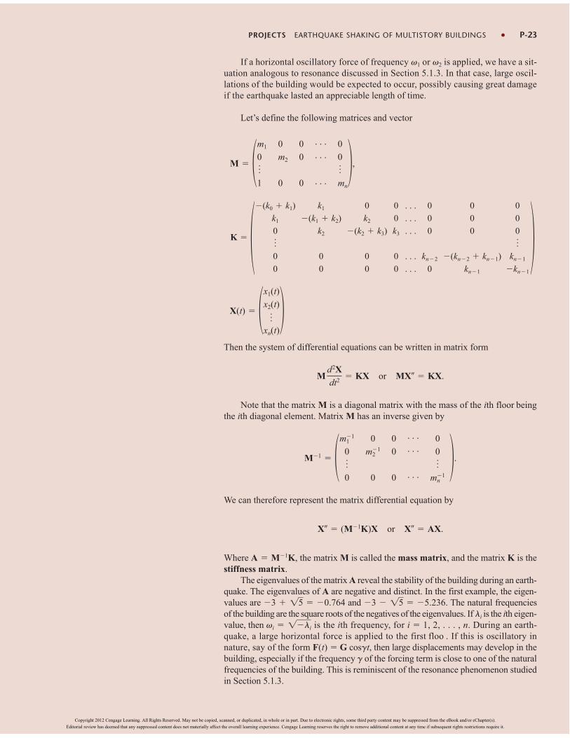
If a horizontal oscillatory force of frequency or is applied, we have a sit-uation analogous to resonance discussed in Section 5.1.3. In that case, large oscil-lations of the building would be expected to occur, possibly causing great damageif the earthquake lasted an appreciable length of time.
Let’s define the following matrices and vector
Then the system of differential equations can be written in matrix form
Note that the matrix M is a diagonal matrix with the mass of the ith floor beingthe ith diagonal element. Matrix M has an inverse given by
.
We can therefore represent the matrix differential equation by
Where the matrix M is called the mass matrix, and the matrix K is thestiffness matrix.
The eigenvalues of the matrix A reveal the stability of the building during an earth-quake. The eigenvalues of A are negative and distinct. In the first example, the eigen-values are and The natural frequenciesof the building are the square roots of the negatives of the eigenvalues. If is the ith eigen-value, then is the ith frequency, for i 1, 2, . . . , n. During an earth-quake, a large horizontal force is applied to the first floo . If this is oscillatory innature, say of the form F(t) G cosgt, then large displacements may develop in thebuilding, especially if the frequency g of the forcing term is close to one of the naturalfrequencies of the building. This is reminiscent of the resonance phenomenon studiedin Section 5.1.3.
vi 1li
li
3 15 5.236.3 15 0.764
A M1K,
X (M1K)X or X AX.
M1 m1
1
0
o0
0
m12
0
0
0
0
. . .
. . .
. . .
0
0
om1
n
Md2X
dt2 KX or MX KX.
X(t) x1(t)
x2(t)
oxn(t)
K (k0 k1)
k1
0
o0
0
k1
(k1 k2)
k2
0
0
0
k2
(k2 k3)
0
0
0
0
k3
0
0
. . .
. . .
. . .
. . .
. . .
0
0
0
kn2
0
0
0
0
(kn2 kn1)
kn1
0
0
0
okn1
kn1
M
m1
0
o1
0
m2
0
0
0
0
. . .
. . .
. . .
0
0
omn
,
v2v1
PROJECTS EARTHQUAKE SHAKING OF MULTISTORY BUILDINGS P-23
Copyright 2012 Cengage Learning. All Rights Reserved. May not be copied, scanned, or duplicated, in whole or in part. Due to electronic rights, some third party content may be suppressed from the eBook and/or eChapter(s).
Editorial review has deemed that any suppressed content does not materially affect the overall learning experience. Cengage Learning reserves the right to remove additional content at any time if subsequent rights restrictions require it.

P-24 PROJECTS EARTHQUAKE SHAKING OF MULTISTORY BUILDINGS
As another example, suppose we have a 10-story building, where each floor has amass 10000 kg, and each ki value is 5000 kg/s2. Then
The eigenvalues of A are found easily using Mathematica or another similar computerpackage. These values are 1.956, 1.826, 1.623, 1.365, 1.075, 0.777,0.5, 0.267, 0.099, and 0.011, with corresponding frequencies 1.399, 1.351,1.274, 1.168, 1.037, 0.881, 0.707, 0.517, 0.315, and 0.105 and periods of oscillation(2p/v) 4.491, 4.651, 4.932, 5.379, 6.059, 7.132, 8.887, 12.153, 19.947, and 59.840.During a typical earthquake whose period might be in the range of 2 to 3 seconds, thisbuilding does not seem to be in any danger of developing resonance. However, ifthe k values were 10 times as large (multiply A by 10), then, for example, the sixthperiod would be 2.253 seconds, while the fifth through seventh are all on the order of2–3 seconds. Such a building is more likely to suffer damage in a typical earthquakeof period 2–3 seconds.
Related Problems1. Consider a three-story building with the same m and k values as in the first exam-
ple. Write down the corresponding system of differential equations. What are thematrices M, K, and A? Find the eigenvalues for A. What range of frequencies ofan earthquake would place the building in danger of destruction?
2. Consider a three-story building with the same m and k values as in the secondexample. Write down the corresponding system of differential equations. Whatare the matrices M, K, and A? Find the eigenvalues for A. What range of fre-quencies of an earthquake would place the building in danger of destruction?
3. Consider the tallest building on your campus. Assume reasonable values for themass of each floor and for the proportionality constants between floors. If youhave trouble coming up with such values, use the ones in the example problems.Find the matrices M, K, and A, and find the eigenvalues of A and the frequen-cies and periods of oscillation. Is your building safe from a modest-sized period-2 earthquake? What if you multiplied the matrix K by 10 (that is, made thebuilding stiffer)? What would you have to multiply the matrix K by in order toput your building in the danger zone?
4. Solve the earthquake problem for the three-story building of Problem 1:
,
where F(t) = G cosgt, G = EB, B = [1 0 0]T, E = 10,000 lbs is the amplitudeof the earthquake force acting at ground level, and g = 3 is the frequency of theearthquake (a typical earthquake frequency). See Section 8.3 for the method ofsolving nonhomogeneous matrix differential equations. Use initial conditionsfor a building at rest.
MX KX F(t)
A M1K 1
0.5
0
0
0
0
0
0
0
0
0.5
1
0.5
0
0
0
0
0
0
0
0
0.5
1
0.5
0
0
0
0
0
0
0
0
0.5
1
0.5
0
0
0
0
0
0
0
0
0.5
1
0.5
0
0
0
0
0
0
0
0
0.5
1
0.5
0
0
0
0
0
0
0
0
0.5
1
0.5
0
0
0
0
0
0
0
0
0.5
1
0.5
0
0
0
0
0
0
0
0
0.5
1
0.5
0
0
0
0
0
0
0
0
0.5
0.5
Copyright 2012 Cengage Learning. All Rights Reserved. May not be copied, scanned, or duplicated, in whole or in part. Due to electronic rights, some third party content may be suppressed from the eBook and/or eChapter(s).
Editorial review has deemed that any suppressed content does not materially affect the overall learning experience. Cengage Learning reserves the right to remove additional content at any time if subsequent rights restrictions require it.

Modeling Arms Racesby Michael Olinick
The last hundred years have seen numerous dangerous, destabilizing, and expensivearms races. The outbreak of World War I climaxed a rapid buildup of armamentsamong rival European powers. There was a similar mutual accumulation of conven-tional arms just prior to World War II. The United States and the Soviet Union en-gaged in a costly nuclear arms race during the forty years of the Cold War. Stockpilingof ever-more deadly weapons is common today in many parts of the world, includingthe Middle East, the Indian subcontinent, and the Korean peninsula.
British meteorologist and educator Lewis F. Richardson (1881–1953) developedseveral mathematical models to analyze the dynamics of arms races, the evolutionover time of the process of interaction between countries in their acquisition ofweapons. Arms race models generally assume that each nation adjusts its accumula-tion of weapons in some manner dependent on the size of its own stockpile and thearmament levels of the other nations.
Richardson’s primary model of a two country arms race is based on mutualfear: A nation is spurred to increase its arms stockpile at a rate proportional to thelevel of armament expenditures of its rival. Richardson’s model takes into accountinternal constraints within a nation that slow down arms buildups: The more anation is spending on arms, the harder it is to make greater increases, because itbecomes increasingly difficult to divert society’s resources from basic needs suchas food and housing to weapons. Richardson also built into his model other factorsdriving or slowing down an arms race that are independent of levels of arms expen-ditures.
The mathematical structure of this model is a linked system of two first-ordelinear differential equations. If x and y represent the amount of wealth being spent onarms by two nations at time t, then the model has the form
where a, b, m, and n are positive constants while r and s are constants which can bepositive or negative. The constants a and b measure mutual fear; the constants m andn represent proportionality factors for the “internal brakes” to further arms increases.Positive values for r and s correspond to underlying factors of ill will or distrust thatwould persist even if arms expenditures dropped to zero. Negative values for r and sindicate a contribution based on goodwill.
The dynamic behavior of this system of differential equations depends on therelative sizes of ab and mn together with the signs of r and s. Although the modelis a relatively simple one, it allows us to consider several different long-term out-comes. It’s possible that two nations might move simultaneously toward mutualdisarmament, with x and y each approaching zero. A vicious cycle of unboundedincreases in x and y is another possible scenario. A third eventuality is that the armsexpenditures asymptotically approach a stable point (x*, y*) regardless of the initiallevel of arms expenditures. In other cases, the eventual outcome depends on thestarting point. Figure 1 shows one possible situation with four different initial
dy
dt bx ny s
dx
dt ay mx r
P-25
Project for Section 8.3
Weapons and ammunition recovered duringmilitary operations against Taliban militantsin South Waziristan in October 2009
NIC
OL
AS
AS
FO
UR
I/A
FP
/Get
ty I
mag
es/N
ewsc
om
Copyright 2012 Cengage Learning. All Rights Reserved. May not be copied, scanned, or duplicated, in whole or in part. Due to electronic rights, some third party content may be suppressed from the eBook and/or eChapter(s).
Editorial review has deemed that any suppressed content does not materially affect the overall learning experience. Cengage Learning reserves the right to remove additional content at any time if subsequent rights restrictions require it.

levels, each of which leads to a “stable outcome,” the intersection of the nullclinesdxdt 0 and dydt 0.
Although “real world” arms races seldom match exactly with Richardson’s model,his pioneering work has led to many fruitful applications of differential equation modelsto problems in international relations and political science. As two leading researchers inthe field note in [3], “The Richardson arms race model constitutes one of the most impor-tant models of arms race phenomena and, at the same time, one of the most influentiaformal models in all of the international relations literature.”
Arms races are not limited to the interaction of nation states. They can take placebetween a government and a paramilitary terrorist group within its borders as, for ex-ample, the Tamil Tigers in Sri Lanka, the Shining Path in Peru, or the Taliban inAfghanistan. Arms phenomena have also been observed between rival urban gangsand between law enforcement agencies and organized crime.
The “arms” need not even be weapons. Colleges have engaged in “amenitiesarms races,” often spending millions of dollars on more luxurious dormitories,state- of-the-art athletic facilities, epicurean dining options, and the like, to be morecompetitive in attracting student applications. Biologists have identified the possi-bility of evolutionary arms races between and within species as an adaptation in onelineage may change the selection pressure on another lineage, giving rise to a counter-adaptation. Most generally, the assumptions represented in a Richardson-typemodel also characterize many competitions in which each side perceives a need tostay ahead of the other in some mutually important measure.
Related Problems1. (a) By substituting the proposed solutions into the differential equations, show
that the solution of the particular Richardson arms model
dy
dt 2x 4y 8
dx
dt y 3x 3
P-26 PROJECTS MODELING ARMS RACES
dx/dt = 0y
x
dy/dt = 0
1
1
0
2
3
4
5
6
2 3 4 5 6
FIGURE 1 Expenditures approaching a stable point
Copyright 2012 Cengage Learning. All Rights Reserved. May not be copied, scanned, or duplicated, in whole or in part. Due to electronic rights, some third party content may be suppressed from the eBook and/or eChapter(s).
Editorial review has deemed that any suppressed content does not materially affect the overall learning experience. Cengage Learning reserves the right to remove additional content at any time if subsequent rights restrictions require it.

with initial condition x(0) 12, y(0) 15 is
What is the long-term behavior of this arms race?
(b) For the Richardson arms race model (a) with arbitrary initial conditionsx(0) A, y(0) B, show that the solution is given by
x(t) Ce5t De2t 2 C (A B 1)3where
y(t) 2Ce5t De2t 3 D (2A B 7)3
Show that this result implies that the qualitative long-term behavior of such anarms race is the same (x(t) : 2, y(t) : 3), no matter what the initial values of xand y are.
2. The qualitative long-term behavior of a Richardson arms race model can, insome cases, depend on the initial conditions. Consider, for example, the system
For each of the given initial conditions below, verify that the proposed solu-tion works and discuss the long-term behavior:(a) x(0) 1, y(0) 1 : x(t) 10 9et, y(t) 10 9et
(b) x(0) 1, y(0) 22 : x(t) 10 9e6t, y(t) 10 12e6t
(c) x(0) 1, y(0) 29 : x(t) 12e6t 3et 10, y(t) 16e6t 3et 10(d) x(0) 10, y(0) 10 : x(t) 10, y(t) 10 for all t
3. (a) As a possible alternative to the Richardson model, consider a stock adjustmentmodel for an arms race. The assumption here is that each country sets a desiredlevel of arms expenditures for itself and then changes its weapons stock pro-portionally to the gap between its current level and the desired one. Show thatthis assumption can be represented by the system of differential equations
where x* and y* are desired constant levels and a, b are positive constants.How will x and y evolve over time under such a model?
(b) Generalize the stock adjustment model of (a) to a more realistic one wherethe desired level for each country depends on the levels of both countries. Inparticular, suppose x* has the form x* c dy where c and d are positiveconstants and that y* has a similar format. Show that, under these assump-tions, the stock adjustment model is equivalent to a Richardson model.
4. Extend the Richardson model to three nations, deriving a system of linear differen-tial equations if the three are mutually fearful: each one is spurred to arm by the ex-penditures of the other two. How might the equations change if two of the nationsare close allies not threatened by the arms buildup of each other, but fearful of thearmaments of the third. Investigate the long-term behavior of such arms races.
5. In the real world, an unbounded runaway arms race is impossible since there isan absolute limit to the amount any country can spend on weapons; e.g. gross na-tional product minus some amount for survival. Modify the Richardson model toincorporate this idea and analyze the dynamics of an arms race governed bythese new differential equations.
dx
dt b(y* y)
dx
dt a(x* x)
dy
dt 4x 3y 10
dx
dt 3y 2x 10
y(t) 32
3e2t
4
3e5t 3
x(t) 32
3e2t
2
3e5t 2
PROJECTS MODELING ARMS RACES P-27
Copyright 2012 Cengage Learning. All Rights Reserved. May not be copied, scanned, or duplicated, in whole or in part. Due to electronic rights, some third party content may be suppressed from the eBook and/or eChapter(s).
Editorial review has deemed that any suppressed content does not materially affect the overall learning experience. Cengage Learning reserves the right to remove additional content at any time if subsequent rights restrictions require it.

References1. Richardson, Lewis F., Arms and Insecurity: A Mathematical Study of the Causes
and Origins of War. Pittsburgh: Boxwood Press, 1960.2. Olinick, Michael, An Introduction to Mathematical Models in the Social and
Life Sciences. Reading, MA: Addison-Wesley, 1978.3. Intriligator, Michael D., and Dagobert L. Brito, “Richardsonian Arms Race
Models” in Manus I. Midlarsky, ed., Handbook of War Studies. Boston: UnwinHyman, 1989.
P-28 PROJECTS MODELING ARMS RACES
ABOUT THE AUTHOR After earning a BA in mathematics and philosophy at the University of Michigan andan MA and PhD from the University of Wisconsin (Madison), Michael Olinickmoved from the Midwest to New England where he joined the Middlebury Collegefaculty in 1970 and now serves as Professor of Mathematics. Dr. Olinick has heldvisiting positions at University College Nairobi, University of California at Berkeley,Wesleyan University, and Lancaster University in Great Britain. He is the author orco-author of a number of books on single and multivariable calculus, mathematicalmodeling, probability, topology, and principles and practice of mathematics. He iscurrently developing a new textbook on mathematical models in the humanities,social, and life sciences.C
ourt
esy
of M
icha
el O
lini
ck
Copyright 2012 Cengage Learning. All Rights Reserved. May not be copied, scanned, or duplicated, in whole or in part. Due to electronic rights, some third party content may be suppressed from the eBook and/or eChapter(s).
Editorial review has deemed that any suppressed content does not materially affect the overall learning experience. Cengage Learning reserves the right to remove additional content at any time if subsequent rights restrictions require it.

1
1.1 Definitions and Terminology
1.2 Initial-Value Problems
1.3 Differential Equations as Mathematical Models
Chapter 1 in Review
The words differential and equations certainly suggest solving some kind of
equation that contains derivatives y, y, . . . . Analogous to a course in algebra and
trigonometry, in which a good amount of time is spent solving equations such as
x2 5x 4 0 for the unknown number x, in this course one of our tasks will be
to solve differential equations such as y 2y y 0 for an unknown function
y (x).
The preceding paragraph tells something, but not the complete story, about
the course you are about to begin. As the course unfolds, you will see that there is
more to the study of differential equations than just mastering methods that
mathematicians over past centuries devised to solve them.
But first things first. In order to read, stu , and be conversant in a specialized
subject, you have to master some of the terminology of that discipline. This is the
thrust of the first two sections of this chapte . In the last section we briefly examin
the link between differential equations and the real world. Practical questions
such as
How fast does a disease spread ? How fast does a population change?
involve rates of change or derivatives. And so the mathematical description—or
mathematical model—of phenomena, experiments, observations, or theories may
be a differential equation.
1 Introduction to Differential Equations
Copyright 2012 Cengage Learning. All Rights Reserved. May not be copied, scanned, or duplicated, in whole or in part. Due to electronic rights, some third party content may be suppressed from the eBook and/or eChapter(s).
Editorial review has deemed that any suppressed content does not materially affect the overall learning experience. Cengage Learning reserves the right to remove additional content at any time if subsequent rights restrictions require it.
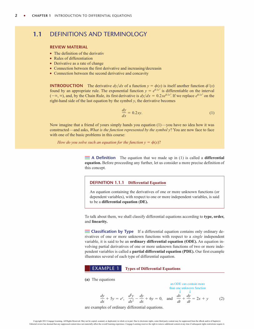
2 CHAPTER 1 INTRODUCTION TO DIFFERENTIAL EQUATIONS
A Definition The equation that we made up in (1) is called a differentialequation. Before proceeding any further, let us consider a more precise definition ofthis concept.
DEFINITION 1.1.1 Differential Equation
An equation containing the derivatives of one or more unknown functions (ordependent variables), with respect to one or more independent variables, is saidto be a differential equation (DE).
To talk about them, we shall classify differential equations according to type, order,and linearity.
Classification by Type If a differential equation contains only ordinary de-rivatives of one or more unknown functions with respect to a single independentvariable, it is said to be an ordinary differential equation (ODE). An equation in-volving partial derivatives of one or more unknown functions of two or more inde-pendent variables is called a partial differential equation (PDE). Our first exampleillustrates several of each type of differential equation.
EXAMPLE 1 Types of Differential Equations
(a) The equationsan ODE can contain more
than one unknown function
(2)
are examples of ordinary differential equations.
dy
dx 5y ex,
d2y
dx2 dy
dx 6y 0, and
dx
dt
dy
dt 2x y
b b
DEFINITIONS AND TERMINOLOGY
REVIEW MATERIAL The definition of the derivativ Rules of differentiation Derivative as a rate of change Connection between the first derivative and increasing/decreasin Connection between the second derivative and concavity
INTRODUCTION The derivative dydx of a function y (x) is itself another function (x)found by an appropriate rule. The exponential function is differentiable on the interval(, ), and, by the Chain Rule, its first derivative is . If we replace on theright-hand side of the last equation by the symbol y, the derivative becomes
. (1)
Now imagine that a friend of yours simply hands you equation (1)—you have no idea how it wasconstructed—and asks, What is the function represented by the symbol y? You are now face to facewith one of the basic problems in this course:
How do you solve such an equation for the function y (x)?
dy
dx 0.2xy
e0.1x2dy>dx 0.2xe0.1x2
y e0.1x2
1.1
Copyright 2012 Cengage Learning. All Rights Reserved. May not be copied, scanned, or duplicated, in whole or in part. Due to electronic rights, some third party content may be suppressed from the eBook and/or eChapter(s).
Editorial review has deemed that any suppressed content does not materially affect the overall learning experience. Cengage Learning reserves the right to remove additional content at any time if subsequent rights restrictions require it.

(b) The following equations are partial differential equations:*
(3)
Notice in the third equation that there are two unknown functions and two indepen-dent variables in the PDE. This means u and v must be functions of two or moreindependent variables.
Notation Throughout this text ordinary derivatives will be written by using
2u
x2 2u
y2 0,2u
x2 2u
t2 2u
t,
u
y
v
x.
1.1 DEFINITIONS AND TERMINOLOGY 3
*Except for this introductory section, only ordinary differential equations are considered in A First Coursein Differential Equations with Modeling Applications, Tenth Edition. In that text the word equation andthe abbreviation DE refer only to ODEs. Partial differential equations or PDEs are considered in theexpanded volume Differential Equations with Boundary-Value Problems, Eighth Edition.
either the Leibniz notation dydx, d2ydx2, d3ydx3, . . . or the prime notation y, y,y, . . . . By using the latter notation, the first two differential equations in (2) can bewritten a little more compactly as y 5y ex and y y 6y 0. Actually, theprime notation is used to denote only the first three derivatives; the fourth derivativeis written y(4) instead of y. In general, the nth derivative of y is written dnydxn ory(n). Although less convenient to write and to typeset, the Leibniz notation has an ad-vantage over the prime notation in that it clearly displays both the dependent andindependent variables. For example, in the equation
it is immediately seen that the symbol x now represents a dependent variable,whereas the independent variable is t. You should also be aware that in physicalsciences and engineering, Newton’s dot notation (derogatorily referred to by someas the “flyspeck” notation) is sometimes used to denote derivatives with respectto time t. Thus the differential equation d2sdt2 32 becomes s 32. Partialderivatives are often denoted by a subscript notation indicating the indepen-dent variables. For example, with the subscript notation the second equation in(3) becomes uxx utt 2ut.
Classification by Order The order of a differential equation (either ODEor PDE) is the order of the highest derivative in the equation. For example,
is a second-order ordinary differential equation. In Example 1, the first and thirdequations in (2) are first-order ODEs, whereas in (3) the first two equations aresecond-order PDEs. First-order ordinary differential equations are occasionally writ-ten in differential form M(x, y) dx N(x, y) dy 0. For example, if we assume thaty denotes the dependent variable in (y x) dx 4x dy 0, then y dydx, so bydividing by the differential dx, we get the alternative form 4xy y x.
In symbols we can express an nth-order ordinary differential equation in onedependent variable by the general form
, (4)
where F is a real-valued function of n 2 variables: x, y, y, . . . , y(n). For both prac-tical and theoretical reasons we shall also make the assumption hereafter that it ispossible to solve an ordinary differential equation in the form (4) uniquely for the
F(x, y, y, . . . , y(n)) 0
first ordersecond order
5( )3
4y exdy–––dx
d 2y––––dx2
d 2x–––dt2
16x 0
unknown functionor dependent variable
independent variable
Copyright 2012 Cengage Learning. All Rights Reserved. May not be copied, scanned, or duplicated, in whole or in part. Due to electronic rights, some third party content may be suppressed from the eBook and/or eChapter(s).
Editorial review has deemed that any suppressed content does not materially affect the overall learning experience. Cengage Learning reserves the right to remove additional content at any time if subsequent rights restrictions require it.
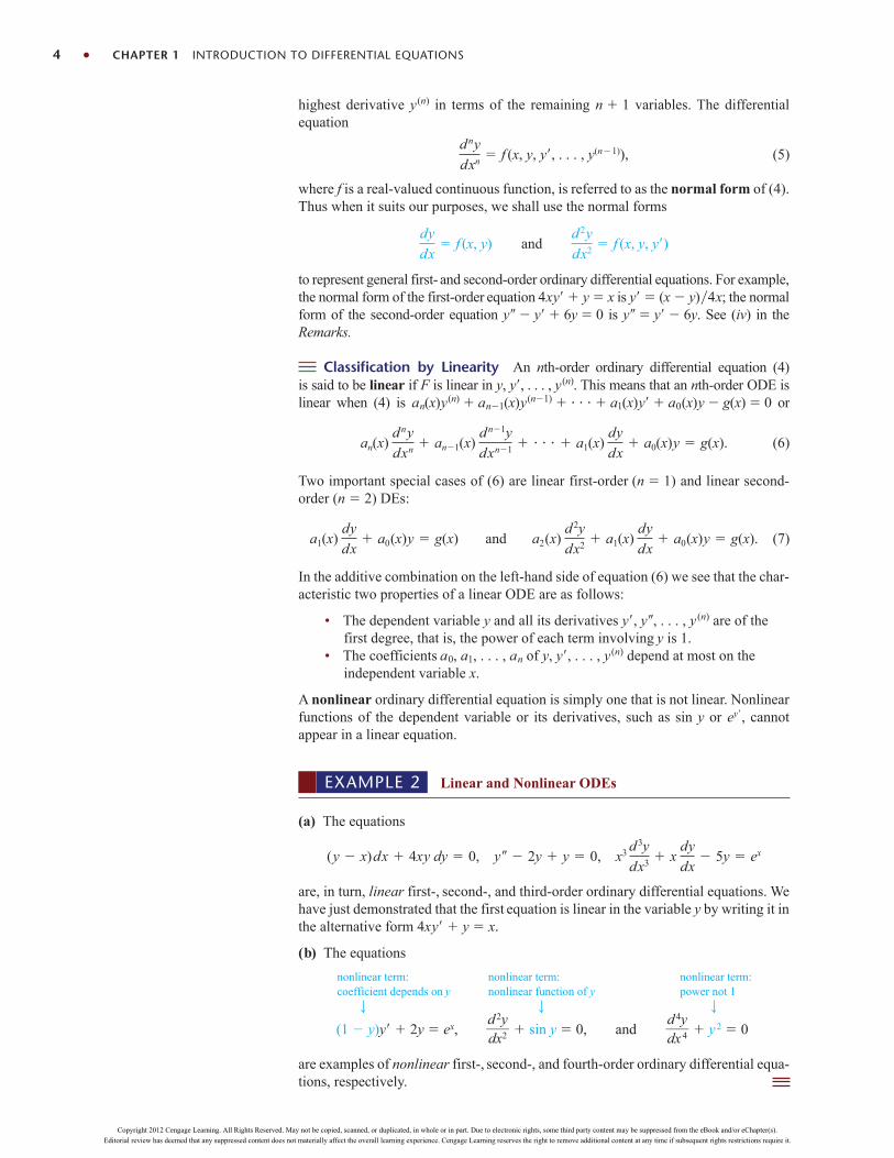
highest derivative y(n) in terms of the remaining n 1 variables. The differentialequation
, (5)
where f is a real-valued continuous function, is referred to as the normal form of (4).Thus when it suits our purposes, we shall use the normal forms
to represent general first- and second-order ordinary differential equations. For example,the normal form of the first-order equation 4xy y x is y (x y)4x; the normalform of the second-order equation y y 6y 0 is y y 6y. See (iv) in theRemarks.
Classification by Linearity An nth-order ordinary differential equation (4)
dy
dx f (x, y) and
d 2y
dx2 f (x, y, y)
dny
dxn f (x, y, y, . . . , y(n1))
4 CHAPTER 1 INTRODUCTION TO DIFFERENTIAL EQUATIONS
EXAMPLE 2 Linear and Nonlinear ODEs
(a) The equations
are, in turn, linear first-, second-, and third-order ordinary differential equations. Wehave just demonstrated that the first equation is linear in the variable y by writing it inthe alternative form 4xy y x.
(b) The equations
are examples of nonlinear first-, second-, and fourth-order ordinary differential equa-tions, respectively.
nonlinear term:coefficient depends on y
nonlinear term:nonlinear function of y
nonlinear term:power not 1
(1 y)y 2y ex, sin y 0, andd 2y––––dx2 y 2 0
d 4y––––dx 4
(y x)dx 4xy dy 0, y 2y y 0, x3 d 3y
dx3 x dy
dx 5y ex
is said to be linear if F is linear in y, y, . . . , y(n). This means that an nth-order ODE islinear when (4) is an(x)y(n) an1(x)y(n1) a1(x)y a0(x)y g(x) 0 or
. (6)
Two important special cases of (6) are linear first-order (n 1) and linear second-order (n 2) DEs:
. (7)
In the additive combination on the left-hand side of equation (6) we see that the char-acteristic two properties of a linear ODE are as follows:
• The dependent variable y and all its derivatives y, y, . . . , y (n) are of thefirst degree, that is, the power of each term involving y is 1.
• The coefficients a0, a1, . . . , an of y, y, . . . , y(n) depend at most on theindependent variable x.
A nonlinear ordinary differential equation is simply one that is not linear. Nonlinearfunctions of the dependent variable or its derivatives, such as sin y or , cannotappear in a linear equation.
ey
a1(x) dy
dx a0(x)y g(x) and a2(x)
d 2y
dx2 a1(x) dy
dx a0(x)y g(x)
an(x) dny
dxn an1(x) dn1y
dxn1 a1(x) dy
dx a0(x)y g(x)
Copyright 2012 Cengage Learning. All Rights Reserved. May not be copied, scanned, or duplicated, in whole or in part. Due to electronic rights, some third party content may be suppressed from the eBook and/or eChapter(s).
Editorial review has deemed that any suppressed content does not materially affect the overall learning experience. Cengage Learning reserves the right to remove additional content at any time if subsequent rights restrictions require it.
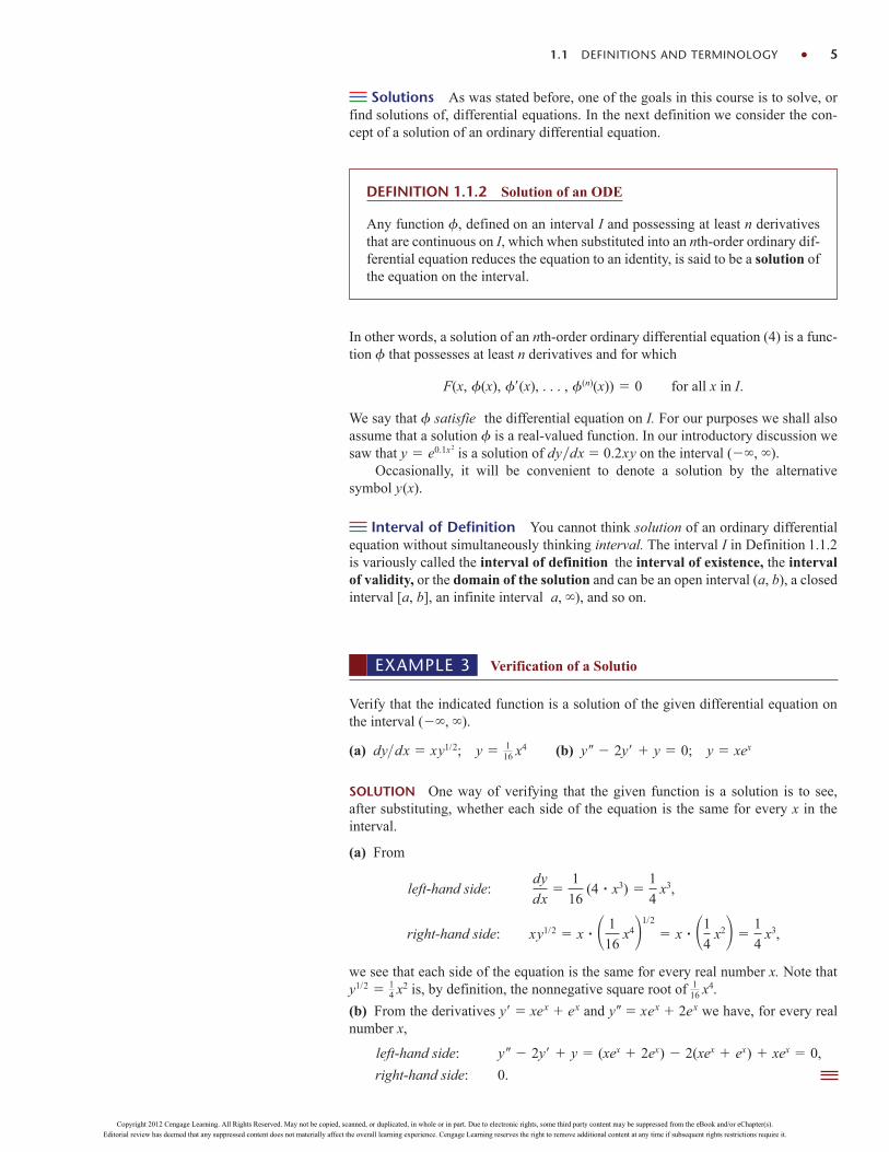
Solutions As was stated before, one of the goals in this course is to solve, orfind solutions of, differential equations. In the next definition we consider the con-cept of a solution of an ordinary differential equation.
1.1 DEFINITIONS AND TERMINOLOGY 5
DEFINITION 1.1.2 Solution of an ODE
Any function , defined on an interval I and possessing at least n derivativesthat are continuous on I, which when substituted into an nth-order ordinary dif-ferential equation reduces the equation to an identity, is said to be a solution ofthe equation on the interval.
In other words, a solution of an nth-order ordinary differential equation (4) is a func-tion that possesses at least n derivatives and for which
We say that satisfie the differential equation on I. For our purposes we shall alsoassume that a solution is a real-valued function. In our introductory discussion wesaw that is a solution of dydx 0.2xy on the interval (, ).
Occasionally, it will be convenient to denote a solution by the alternativesymbol y(x).
Interval of Definition You cannot think solution of an ordinary differentialequation without simultaneously thinking interval. The interval I in Definition 1.1.2is variously called the interval of definition the interval of existence, the intervalof validity, or the domain of the solution and can be an open interval (a, b), a closedinterval [a, b], an infinite interval a, ), and so on.
y e0.1x2
F(x, (x), (x), . . . , (n)(x)) 0 for all x in I.
EXAMPLE 3 Verification of a Solutio
Verify that the indicated function is a solution of the given differential equation onthe interval (, ).
(a) (b)
SOLUTION One way of verifying that the given function is a solution is to see,after substituting, whether each side of the equation is the same for every x in theinterval.
(a) From
we see that each side of the equation is the same for every real number x. Note thatis, by definition, the nonnegative square root of .
(b) From the derivatives y xex ex and y xex 2ex we have, for every realnumber x,
right-hand side: 0.
left-hand side: y 2y y (xex 2ex) 2(xex ex) xex 0,
116 x
4y1/2 14 x
2
right-hand side: xy1/2 x 1
16 x4
1/2
x 1
4 x2
1
4 x3,
left-hand side: dy
dx
1
16 (4 x3)
1
4 x3,
y 2y y 0; y xexdy>dx xy1/2; y 116 x
4
Copyright 2012 Cengage Learning. All Rights Reserved. May not be copied, scanned, or duplicated, in whole or in part. Due to electronic rights, some third party content may be suppressed from the eBook and/or eChapter(s).
Editorial review has deemed that any suppressed content does not materially affect the overall learning experience. Cengage Learning reserves the right to remove additional content at any time if subsequent rights restrictions require it.

Note, too, that in Example 3 each differential equation possesses the constant so-lution y 0, x . A solution of a differential equation that is identicallyzero on an interval I is said to be a trivial solution.
Solution Curve The graph of a solution of an ODE is called a solutioncurve. Since is a differentiable function, it is continuous on its interval I of definition. Thus there may be a difference between the graph of the function and thegraph of the solution . Put another way, the domain of the function need not bethe same as the interval I of definition (or domain) of the solution . Example 4illustrates the difference.
6 CHAPTER 1 INTRODUCTION TO DIFFERENTIAL EQUATIONS
1
x
y
1
(a) function y 1/x, x 0
(b) solution y 1/x, (0, )
1
x
y
1
FIGURE 1.1.1 In Example 4 thefunction y 1x is not the same as thesolution y 1x
EXAMPLE 4 Function versus Solution
The domain of y 1x, considered simply as a function, is the set of all realnumbers x except 0. When we graph y 1x, we plot points in the xy-plane cor-responding to a judicious sampling of numbers taken from its domain. The ratio-nal function y 1x is discontinuous at 0, and its graph, in a neighborhood ofthe origin, is given in Figure 1.1.1(a). The function y 1x is not differentiable atx 0, since the y-axis (whose equation is x 0) is a vertical asymptote of thegraph.
Now y 1x is also a solution of the linear first-order differential equationxy y 0. (Verify.) But when we say that y 1x is a solution of this DE, wemean that it is a function defined on an interval I on which it is differentiable andsatisfies the equation. In other words, y 1x is a solution of the DE on any inter-val that does not contain 0, such as (3, 1), , (, 0), or (0, ). Becausethe solution curves defined by y 1x for 3 x 1 and are sim-ply segments, or pieces, of the solution curves defined by y 1x for x 0and 0 x , respectively, it makes sense to take the interval I to be as large aspossible. Thus we take I to be either (, 0) or (0, ). The solution curve on (0, )is shown in Figure 1.1.1(b).
Explicit and Implicit Solutions You should be familiar with the termsexplicit functions and implicit functions from your study of calculus. A solution inwhich the dependent variable is expressed solely in terms of the independentvariable and constants is said to be an explicit solution. For our purposes, let usthink of an explicit solution as an explicit formula y (x) that we can manipulate,evaluate, and differentiate using the standard rules. We have just seen in the last twoexamples that , y xex, and y 1x are, in turn, explicit solutionsof dydx xy1/2, y 2y y 0, and xy y 0. Moreover, the trivial solu-tion y 0 is an explicit solution of all three equations. When we get down tothe business of actually solving some ordinary differential equations, you willsee that methods of solution do not always lead directly to an explicit solutiony (x). This is particularly true when we attempt to solve nonlinear first-ordedifferential equations. Often we have to be content with a relation or expressionG(x, y) 0 that defines a solution implicitly.
y 116 x
4
12 x 10
(12, 10)
DEFINITION 1.1.3 Implicit Solution of an ODE
A relation G(x, y) 0 is said to be an implicit solution of an ordinarydifferential equation (4) on an interval I, provided that there exists at least onefunction that satisfies the relation as well as the differential equation on I.
Copyright 2012 Cengage Learning. All Rights Reserved. May not be copied, scanned, or duplicated, in whole or in part. Due to electronic rights, some third party content may be suppressed from the eBook and/or eChapter(s).
Editorial review has deemed that any suppressed content does not materially affect the overall learning experience. Cengage Learning reserves the right to remove additional content at any time if subsequent rights restrictions require it.

It is beyond the scope of this course to investigate the conditions under which arelation G(x, y) 0 defines a differentiable function . So we shall assume that ifthe formal implementation of a method of solution leads to a relation G(x, y) 0,then there exists at least one function that satisfies both the relation (that is,G(x, (x)) 0) and the differential equation on an interval I. If the implicit solutionG(x, y) 0 is fairly simple, we may be able to solve for y in terms of x and obtainone or more explicit solutions. See (i) in the Remarks.
1.1 DEFINITIONS AND TERMINOLOGY 7
y
x5
5
y
x5
5
y
x
5
5
−5
(a) implicit solution
x2 y2 25
(b) explicit solution
y1 25 x2, 5 x 5
(c) explicit solution
y2 25 x2, 5 x 5
(a)
FIGURE 1.1.2 An implicit solutionand two explicit solutions of (8) inExample 5
FIGURE 1.1.3 Some solutions of DEin part (a) of Example 6
y
x
c>0
c<0
c=0
EXAMPLE 5 Verification of an Implicit Solutio
The relation x2 y2 25 is an implicit solution of the differential equation
(8)
on the open interval (5, 5). By implicit differentiation we obtain
.
Solving the last equation for the symbol dydx gives (8). Moreover, solvingx2 y2 25 for y in terms of x yields . The two functions
and satisfy the relation (that is,x2 1
2 25 and x2 22 25) and are explicit solutions defined on the interval
(5, 5). The solution curves given in Figures 1.1.2(b) and 1.1.2(c) are segments ofthe graph of the implicit solution in Figure 1.1.2(a).
Any relation of the form x2 y2 c 0 formally satisfies (8) for any constant c.However, it is understood that the relation should always make sense in the real numbersystem; thus, for example, if c 25, we cannot say that x2 y2 25 0 is animplicit solution of the equation. (Why not?)
Because the distinction between an explicit solution and an implicit solutionshould be intuitively clear, we will not belabor the issue by always saying, “Here isan explicit (implicit) solution.”
Families of Solutions The study of differential equations is similar to that ofintegral calculus. In some texts a solution is sometimes referred to as an integralof the equation, and its graph is called an integral curve. When evaluating an anti-derivative or indefinite integral in calculus, we use a single constant c of integration.Analogously, when solving a first-order differential equation F(x, y, y) 0, weusually obtain a solution containing a single arbitrary constant or parameter c. Asolution containing an arbitrary constant represents a set G(x, y, c) 0 of solutionscalled a one-parameter family of solutions. When solving an nth-order differentialequation F(x, y, y, . . . , y(n)) 0, we seek an n-parameter family of solutionsG(x, y, c1, c2, . . . , cn) 0. This means that a single differential equation can possessan infinite number of solutions corresponding to the unlimited number of choicesfor the parameter(s). A solution of a differential equation that is free of arbitraryparameters is called a particular solution.
y 2(x) 125 x2y 1(x) 125 x2
y 225 x2
d
dx x2
d
dx y2
d
dx 25 or 2x 2y
dy
dx 0
dy
dx
x
y
EXAMPLE 6 Particular Solutions
(a) The one-parameter family is an explicit solution of the linearfirst-order equation
on the interval (, ). (Verify.) Figure 1.1.3 shows the graphs of some particularsolutions in this family for various choices of c. The solution y x cos x, the bluegraph in the figure, is a particular solution corresponding to c 0.
xy y x2 sin x
y cx x cos x
Copyright 2012 Cengage Learning. All Rights Reserved. May not be copied, scanned, or duplicated, in whole or in part. Due to electronic rights, some third party content may be suppressed from the eBook and/or eChapter(s).
Editorial review has deemed that any suppressed content does not materially affect the overall learning experience. Cengage Learning reserves the right to remove additional content at any time if subsequent rights restrictions require it.

(b) The two-parameter family y c1ex c2xex is an explicit solution of the linearsecond-order equation
y 2y y 0
in part (b) of Example 3. (Verify.) In Figure 1.1.4 we have shown seven of the “dou-ble infinity” of solutions in the family. The solution curves in red, green, and blueare the graphs of the particular solutions y 5xex (cl 0, c2 5), y 3ex (cl 3,c2 0), and y 5ex 2xex (c1 5, c2 2), respectively.
Sometimes a differential equation possesses a solution that is not a member of afamily of solutions of the equation—that is, a solution that cannot be obtained by spe-cializing any of the parameters in the family of solutions. Such an extra solution is calleda singular solution. For example, we have seen that and y 0 are solutions ofthe differential equation dydx xy1/2 on (, ). In Section 2.2 we shall demonstrate,by actually solving it, that the differential equation dydx xy1/2 possesses the one-parameter family of solutions . When c 0, the resulting particularsolution is . But notice that the trivial solution y 0 is a singular solution, sinceit is not a member of the family ; there is no way of assigning a value tothe constant c to obtain y 0.
In all the preceding examples we used x and y to denote the independent anddependent variables, respectively. But you should become accustomed to seeingand working with other symbols to denote these variables. For example, we coulddenote the independent variable by t and the dependent variable by x.
y (14 x
2 c)2y 1
16 x4y (1
4 x2 c)2
y 116 x4
8 CHAPTER 1 INTRODUCTION TO DIFFERENTIAL EQUATIONS
FIGURE 1.1.5 Some solutions of DEin Example 8
(a) two explicit solutions
(b) piecewise-defined solution
c = 1
c = −1x
y
c = 1,x 0≤
c = −1,x < 0
x
y
FIGURE 1.1.4 Some solutionsof DE in part (b) of Example 6
y
x
EXAMPLE 7 Using Different Symbols
The functions x c1 cos 4t and x c2 sin 4t, where c1 and c2 are arbitrary constantsor parameters, are both solutions of the linear differential equation
For x c1 cos 4t the first two derivatives with respect to t are x 4c1 sin 4tand x 16c1 cos 4t. Substituting x and x then gives
In like manner, for x c2 sin 4t we have x 16c2 sin 4t, and so
Finally, it is straightforward to verify that the linear combination of solutions, or thetwo-parameter family x c1 cos 4t c2 sin 4t, is also a solution of the differentialequation.
The next example shows that a solution of a differential equation can be apiecewise-defined function
x 16x 16c2 sin 4t 16(c2 sin 4t) 0.
x 16x 16c1 cos 4t 16(c1 cos 4t) 0.
x 16x 0.
EXAMPLE 8 Piecewise-Defined Solutio
The one-parameter family of quartic monomial functions y cx4 is an explicit solu-tion of the linear first-order equatio
xy 4y 0
on the interval (, ). (Verify.) The blue and red solution curves shown inFigure 1.1.5(a) are the graphs of y x4 and y x4 and correspond to the choicesc 1 and c 1, respectively.
Copyright 2012 Cengage Learning. All Rights Reserved. May not be copied, scanned, or duplicated, in whole or in part. Due to electronic rights, some third party content may be suppressed from the eBook and/or eChapter(s).
Editorial review has deemed that any suppressed content does not materially affect the overall learning experience. Cengage Learning reserves the right to remove additional content at any time if subsequent rights restrictions require it.

The piecewise-defined di ferentiable function
is also a solution of the differential equation but cannot be obtained from the familyy cx4 by a single choice of c. As seen in Figure 1.1.5(b) the solution is constructedfrom the family by choosing c 1 for x 0 and c 1 for x 0.
Systems of Differential Equations Up to this point we have beendiscussing single differential equations containing one unknown function. Butoften in theory, as well as in many applications, we must deal with systems ofdifferential equations. A system of ordinary differential equations is two or moreequations involving the derivatives of two or more unknown functions of a singleindependent variable. For example, if x and y denote dependent variables and tdenotes the independent variable, then a system of two first-orde differentialequations is given by
(9)
A solution of a system such as (9) is a pair of differentiable functions x 1(t),y 2(t), defined on a common interval I, that satisfy each equation of the systemon this interval.
dy
dt g(t, x, y).
dx
dt f(t, x, y)
y x4, x 0
x4, x 0
1.1 DEFINITIONS AND TERMINOLOGY 9
REMARKS
(i) A few last words about implicit solutions of differential equations are inorder. In Example 5 we were able to solve the relation x2 y2 25 fory in terms of x to get two explicit solutions, and
, of the differential equation (8). But don’t read too muchinto this one example. Unless it is easy or important or you are instructed to,there is usually no need to try to solve an implicit solution G(x, y) 0 for yexplicitly in terms of x. Also do not misinterpret the second sentence followingDefinition 1.1.3. An implicit solution G(x, y) 0 can define a perfectly gooddifferentiable function that is a solution of a DE, yet we might not be able tosolve G(x, y) 0 using analytical methods such as algebra. The solution curveof may be a segment or piece of the graph of G(x, y) 0. See Problems 45and 46 in Exercises 1.1. Also, read the discussion following Example 4 inSection 2.2.
(ii) Although the concept of a solution has been emphasized in this section,you should also be aware that a DE does not necessarily have to possessa solution. See Problem 39 in Exercises 1.1. The question of whether asolution exists will be touched on in the next section.
(iii) It might not be apparent whether a first-order ODE written in differentialform M(x, y)dx N(x, y)dy 0 is linear or nonlinear because there is nothingin this form that tells us which symbol denotes the dependent variable. SeeProblems 9 and 10 in Exercises 1.1.
(iv) It might not seem like a big deal to assume that F(x, y, y, . . . , y (n)) 0 canbe solved for y(n), but one should be a little bit careful here. There are exceptions,and there certainly are some problems connected with this assumption. SeeProblems 52 and 53 in Exercises 1.1.
(v) You may run across the term closed form solutions in DE texts or inlectures in courses in differential equations. Translated, this phrase usually
2(x) 125 x21(x) 125 x2
Copyright 2012 Cengage Learning. All Rights Reserved. May not be copied, scanned, or duplicated, in whole or in part. Due to electronic rights, some third party content may be suppressed from the eBook and/or eChapter(s).
Editorial review has deemed that any suppressed content does not materially affect the overall learning experience. Cengage Learning reserves the right to remove additional content at any time if subsequent rights restrictions require it.

10 CHAPTER 1 INTRODUCTION TO DIFFERENTIAL EQUATIONS
refers to explicit solutions that are expressible in terms of elementary (orfamiliar) functions: finite combinations of integer powers of x, roots, exponen-tial and logarithmic functions, and trigonometric and inverse trigonometricfunctions.
(vi) If every solution of an nth-order ODE F(x, y, y, . . . , y(n)) 0 on an inter-val I can be obtained from an n-parameter family G(x, y, c1, c2, . . . , cn) 0 byappropriate choices of the parameters ci, i 1, 2, . . . , n, we then say that thefamily is the general solution of the DE. In solving linear ODEs, we shall im-pose relatively simple restrictions on the coefficients of the equation; with theserestrictions one can be assured that not only does a solution exist on an intervalbut also that a family of solutions yields all possible solutions. Nonlinear ODEs,with the exception of some first-order equations, are usually difficult or impos-sible to solve in terms of elementary functions. Furthermore, if we happen toobtain a family of solutions for a nonlinear equation, it is not obvious whetherthis family contains all solutions. On a practical level, then, the designation“general solution” is applied only to linear ODEs. Don’t be concerned aboutthis concept at this point, but store the words “general solution” in the back ofyour mind—we will come back to this notion in Section 2.3 and again inChapter 4.
EXERCISES 1.1 Answers to selected odd-numbered problems begin on page ANS-1.
In Problems 1–8 state the order of the given ordinary differ-ential equation. Determine whether the equation is linear ornonlinear by matching it with (6).
1. (1 x)y 4xy 5y cos x
2.
3. t5y(4) t3y 6y 0
4.
5.
6.
7. (sin )y (cos )y 2
8.
In Problems 9 and 10 determine whether the given first-order differential equation is linear in the indicateddependent variable by matching it with the first differentialequation given in (7).
9. (y2 1) dx x dy 0; in y; in x
10. u dv (v uv ueu) du 0; in v; in u
x 1 x. 2
3 x. x 0
d 2R
dt 2 k
R2
d 2y
dx 2 B1 dy
dx2
d 2u
dr 2 du
dr u cos(r u)
x d3y
dx3 dy
dx4
y 0
In Problems 11–14 verify that the indicated function is anexplicit solution of the given differential equation. Assumean appropriate interval I of definition for each solution
11. 2y y 0; y ex/2
12.
13. y 6y 13y 0; y e3x cos 2x
14. y y tan x; y (cos x)ln(sec x tan x)
In Problems 15–18 verify that the indicated function y (x) is an explicit solution of the given first-ordedifferential equation. Proceed as in Example 2, by consider-ing simply as a function, give its domain. Then by consid-ering as a solution of the differential equation, give at leastone interval I of definition
15.
16. y 25 y2; y 5 tan 5x
17. y 2xy2; y 1(4 x2)
18. 2y y3 cos x; y (1 sin x)1/2
In Problems 19 and 20 verify that the indicated expression isan implicit solution of the given first-order differential equa-tion. Find at least one explicit solution y (x) in each case.
(y x)y y x 8; y x 42x 2
dy
dt 20y 24; y
6
5
6
5 e20t
Copyright 2012 Cengage Learning. All Rights Reserved. May not be copied, scanned, or duplicated, in whole or in part. Due to electronic rights, some third party content may be suppressed from the eBook and/or eChapter(s).
Editorial review has deemed that any suppressed content does not materially affect the overall learning experience. Cengage Learning reserves the right to remove additional content at any time if subsequent rights restrictions require it.

Use a graphing utility to obtain the graph of an explicit solu-tion. Give an interval I of definition of each solution .
19.
20. 2xy dx (x2 y) dy 0; 2x2y y2 1
In Problems 21–24 verify that the indicated family of func-tions is a solution of the given differential equation. Assumean appropriate interval I of definition for each solution
21.
22.
23.
24.
25. Verify that the piecewise-defined functio
is a solution of the differential equation xy 2y 0on (, ).
26. In Example 5 we saw that y 1(x) andare solutions of dydx
xy on the interval (5, 5). Explain why the piecewise-defined functio
is not a solution of the differential equation on theinterval (5, 5).
In Problems 27–30 find values of m so that the functiony emx is a solution of the given differential equation.
27. y 2y 0 28. 5y 2y
29. y 5y 6y 0 30. 2y 7y 4y 0
In Problems 31 and 32 find values of m so that the functiony xm is a solution of the given differential equation.
31. xy 2y 0
32. x2y 7xy 15y 0
y 125 x2,
125 x2,
5 x 0
0 x 5
y 2(x) 125 x2125 x2
y x2, x 0
x2, x 0
y c1x1 c2x c3x ln x 4x2
x3 d3y
dx3 2x2 d2y
dx2 x dy
dx y 12x2;
d 2y
dx2 4 dy
dx 4y 0; y c1e2x c2xe2x
dy
dx 2xy 1; y ex2x
0 et2
dt c1ex2
dP
dt P(1 P); P
c1et
1 c1et
dX
dt (X 1)(1 2X); ln2X 1
X 1 t
1.1 DEFINITIONS AND TERMINOLOGY 11
In Problems 33–36 use the concept that y c, x ,is a constant function if and only if y 0 to determinewhether the given differential equation possesses constantsolutions.
33. 3xy 5y 10
34. y y2 2y 3
35. (y 1)y 1
36. y 4y 6y 10
In Problems 37 and 38 verify that the indicated pair offunctions is a solution of the given system of differentialequations on the interval (, ).
37. 38.
,
Discussion Problems
39. Make up a differential equation that does not possessany real solutions.
40. Make up a differential equation that you feel confidenpossesses only the trivial solution y 0. Explain yourreasoning.
41. What function do you know from calculus is such thatits first derivative is itself? Its first derivative is aconstant multiple k of itself? Write each answer inthe form of a first-order differential equation with asolution.
42. What function (or functions) do you know from calcu-lus is such that its second derivative is itself? Its secondderivative is the negative of itself? Write each answer inthe form of a second-order differential equation with asolution.
43. Given that y sin x is an explicit solution of the first-
order differential equation . Find an in-
terval I of definition [Hint: I is not the interval (, ).]
44. Discuss why it makes intuitive sense to presume thatthe linear differential equation y 2y 4y 5 sin thas a solution of the form y A sin t B cos t, whereA and B are constants. Then find specific constants Aand B so that y A sin t B cos t is a particular solu-tion of the DE.
dy
dx 11 y2
y cos 2t sin 2t 15 ety e2t 5e6t
x cos 2t sin 2t 15 etx e2t 3e6t,
d 2y
dt 2 4x et;dy
dt 5x 3y;
d 2x
dt 2 4y etdx
dt x 3y
Copyright 2012 Cengage Learning. All Rights Reserved. May not be copied, scanned, or duplicated, in whole or in part. Due to electronic rights, some third party content may be suppressed from the eBook and/or eChapter(s).
Editorial review has deemed that any suppressed content does not materially affect the overall learning experience. Cengage Learning reserves the right to remove additional content at any time if subsequent rights restrictions require it.

In Problems 45 and 46 the given figure represents the graphof an implicit solution G(x, y) 0 of a differential equationdydx f (x, y). In each case the relation G(x, y) 0implicitly defines several solutions of the DE. Carefullyreproduce each figure on a piece of paper. Use differentcolored pencils to mark off segments, or pieces, on eachgraph that correspond to graphs of solutions. Keep in mindthat a solution must be a function and differentiable. Usethe solution curve to estimate an interval I of definition ofeach solution .
45.
12 CHAPTER 1 INTRODUCTION TO DIFFERENTIAL EQUATIONS
51. Discuss, and illustrate with examples, how to solvedifferential equations of the forms dydx f (x) andd2ydx2 f (x).
52. The differential equation x(y)2 4y 12x3 0 hasthe form given in (4). Determine whether the equationcan be put into the normal form dydx f (x, y).
53. The normal form (5) of an nth-order differential equa-tion is equivalent to (4) whenever both forms haveexactly the same solutions. Make up a first-order differ-ential equation for which F(x, y, y) 0 is not equiva-lent to the normal form dydx f (x, y).
54. Find a linear second-order differential equation F(x, y, y, y) 0 for which y c1x c2x2 is a two-parameter family of solutions. Make sure that your equa-tion is free of the arbitrary parameters c1 and c2.
Qualitative information about a solution y (x) of adifferential equation can often be obtained from theequation itself. Before working Problems 55–58, recallthe geometric significance of the derivatives dydxand d2ydx2.
55. Consider the differential equation .
(a) Explain why a solution of the DE must be anincreasing function on any interval of the x-axis.
(b) What are What does
this suggest about a solution curve as
(c) Determine an interval over which a solution curve isconcave down and an interval over which the curveis concave up.
(d) Sketch the graph of a solution y (x) of the dif-ferential equation whose shape is suggested byparts (a)– (c).
56. Consider the differential equation dydx 5 y.
(a) Either by inspection or by the method suggested inProblems 33–36, find a constant solution of the DE.
(b) Using only the differential equation, find intervals onthe y-axis on which a nonconstant solution y (x)is increasing. Find intervals on the y-axis on which y (x) is decreasing.
57. Consider the differential equation dydx y(a by),where a and b are positive constants.
(a) Either by inspection or by the method suggestedin Problems 33–36, find two constant solutions ofthe DE.
(b) Using only the differential equation, find intervals onthe y-axis on which a nonconstant solution y (x)is increasing. Find intervals on which y (x) isdecreasing.
(c) Using only the differential equation, explain why y a2b is the y-coordinate of a point of inflectioof the graph of a nonconstant solution y (x).
x : ?
limx :
dy>dx and limx :
dy>dx?
dy>dx ex2
FIGURE 1.1.6 Graph for Problem 45
FIGURE 1.1.7 Graph for Problem 46
y
x
1
1
1 x
1
y46.
47. The graphs of members of the one-parameter familyx3 y3 3cxy are called folia of Descartes. Verifythat this family is an implicit solution of the first-ordedifferential equation
48. The graph in Figure 1.1.7 is the member of the family offolia in Problem 47 corresponding to c 1. Discuss:How can the DE in Problem 47 help in finding pointson the graph of x3 y3 3xy where the tangent lineis vertical? How does knowing where a tangent line isvertical help in determining an interval I of definitioof a solution of the DE? Carry out your ideas,and compare with your estimates of the intervals inProblem 46.
49. In Example 5 the largest interval I over which theexplicit solutions y 1(x) and y 2(x) are defineis the open interval (5, 5). Why can’t the interval I ofdefinition be the closed interval 5, 5]?
50. In Problem 21 a one-parameter family of solutions ofthe DE P P(1 P) is given. Does any solutioncurve pass through the point (0, 3)? Through thepoint (0, 1)?
dy
dx
y(y3 2x3)
x(2y3 x3).
Copyright 2012 Cengage Learning. All Rights Reserved. May not be copied, scanned, or duplicated, in whole or in part. Due to electronic rights, some third party content may be suppressed from the eBook and/or eChapter(s).
Editorial review has deemed that any suppressed content does not materially affect the overall learning experience. Cengage Learning reserves the right to remove additional content at any time if subsequent rights restrictions require it.

1.2 INITIAL-VALUE PROBLEMS 13
(d) On the same coordinate axes, sketch the graphs ofthe two constant solutions found in part (a). Theseconstant solutions partition the xy-plane into threeregions. In each region, sketch the graph of a non-constant solution y (x) whose shape is sug-gested by the results in parts (b) and (c).
58. Consider the differential equation y y2 4.
(a) Explain why there exist no constant solutions ofthe DE.
(b) Describe the graph of a solution y (x). Forexample, can a solution curve have any relativeextrema?
(c) Explain why y 0 is the y-coordinate of a point ofinflection of a solution curve
(d) Sketch the graph of a solution y (x) of thedifferential equation whose shape is suggested byparts (a)–(c).
Computer Lab Assignments
In Problems 59 and 60 use a CAS to compute all derivativesand to carry out the simplifications needed to verify that theindicated function is a particular solution of the given differ-ential equation.
59. y(4) 20y 158y 580y 841y 0;
y xe5x cos 2x
60.
y 20 cos(5 ln x)
x 3
sin(5 ln x)
x
x3y 2x2y 20xy 78y 0;
Geometric Interpretation of IVPs The cases n 1 and n 2 in (1),
(2) Subject to: y(x0) y0
Solve: dy
dx f (x, y)
INITIAL-VALUE PROBLEMS
REVIEW MATERIAL Normal form of a DE Solution of a DE Family of solutions
INTRODUCTION We are often interested in problems in which we seek a solution y(x) of adifferential equation so that y(x) also satisfies certain prescribed side conditions—that is, conditionsthat are imposed on the unknown function y(x) and its derivatives at a point x0. On some interval Icontaining x0 the problem of solving an nth-order differential equation subject to n side conditionsspecified at x0:
(1)
where y0, y1, . . . , yn1 are arbitrary real constants, is called an nth-order initial-valueproblem (IVP). The values of y(x) and its first n 1 derivatives at x0, y(x0) y0, y(x0) y1, . . . ,y(n1)(x0) yn1 are called initial conditions (IC).
Solving an nth-order initial-value problem such as (1) frequently entails first finding an n-parameter family of solutions of the given differential equation and then using the initial-conditions at x0 to determine the n constants in this family. The resulting particular solution isdefined on some interval I containing the initial point x0.
Subject to: y(x0) y0, y(x0) y1, . . . , y(n1)(x0) yn1,
Solve: dny
dxn f x, y, y, . . . , y(n1)
1.2
Copyright 2012 Cengage Learning. All Rights Reserved. May not be copied, scanned, or duplicated, in whole or in part. Due to electronic rights, some third party content may be suppressed from the eBook and/or eChapter(s).
Editorial review has deemed that any suppressed content does not materially affect the overall learning experience. Cengage Learning reserves the right to remove additional content at any time if subsequent rights restrictions require it.

and (3)
are examples of first and second-order initial-value problems, respectively. Thesetwo problems are easy to interpret in geometric terms. For (2) we are seeking a solutiony(x) of the differential equation y f (x, y) on an interval I containing x0 so that itsgraph passes through the specified point (x0, y0). A solution curve is shown in bluein Figure 1.2.1. For (3) we want to find a solution y(x) of the differential equation y f (x, y, y) on an interval I containing x0 so that its graph not only passes through(x0, y0) but the slope of the curve at this point is the number y1. A solution curve isshown in blue in Figure 1.2.2. The words initial conditions derive from physical sys-tems where the independent variable is time t and where y(t0) y0 and y(t0) y1 rep-resent the position and velocity, respectively, of an object at some beginning, or initial,time t0.
Subject to: y(x0) y0, y(x0) y1
Solve: d2y
dx2 f (x, y, y)
14 CHAPTER 1 INTRODUCTION TO DIFFERENTIAL EQUATIONS
FIGURE 1.2.3 Solution curves of twoIVPs in Example 1
y
x
(0, 3)
(1, −2)
FIGURE 1.2.1 Solution curve offirst-orde IVP
FIGURE 1.2.2 Solution curve ofsecond-order IVP
xI
solutions of the DE
( x 0 , y 0 )
y
m = y 1
xI
solutions of the DE
( x 0 , y 0 )
y
EXAMPLE 1 Two First-Order IVPs
(a) In Problem 41 in Exercises 1.1 you were asked to deduce that y cex is a one-parameter family of solutions of the simple first-order equation y y. All thesolutions in this family are defined on the interval (, ). If we impose an initialcondition, say, y(0) 3, then substituting x 0, y 3 in the family determines theconstant 3 ce0 c. Thus y 3ex is a solution of the IVP
(b) Now if we demand that a solution curve pass through the point (1, 2) ratherthan (0, 3), then y(1) 2 will yield 2 ce or c 2e1. In this case y 2ex1 is a solution of the IVP
The two solution curves are shown in dark blue and dark red in Figure 1.2.3.
The next example illustrates another first-order initial-value problem. In thisexample notice how the interval I of definition of the solution y(x) depends on theinitial condition y(x0) y0.
y y, y(1) 2.
y y, y(0) 3.
EXAMPLE 2 Interval I of Definition of a Solutio
In Problem 6 of Exercises 2.2 you will be asked to show that a one-parameter familyof solutions of the first-order differential equation y 2xy2 0 is y 1(x2 c).If we impose the initial condition y(0) 1, then substituting x 0 and y 1into the family of solutions gives 1 1c or c 1. Thus y 1(x2 1). Wenow emphasize the following three distinctions:
• Considered as a function, the domain of y 1(x2 1) is the set of realnumbers x for which y(x) is defined; this is the set of all real numberexcept x 1 and x 1. See Figure 1.2.4(a).
• Considered as a solution of the differential equation y 2xy2 0, theinterval I of definition of y 1(x2 1) could be taken to be anyinterval over which y(x) is defined and di ferentiable. As can be seen inFigure 1.2.4(a), the largest intervals on which y 1(x2 1) is a solutionare (,1), (1, 1), and (1, ).
Copyright 2012 Cengage Learning. All Rights Reserved. May not be copied, scanned, or duplicated, in whole or in part. Due to electronic rights, some third party content may be suppressed from the eBook and/or eChapter(s).
Editorial review has deemed that any suppressed content does not materially affect the overall learning experience. Cengage Learning reserves the right to remove additional content at any time if subsequent rights restrictions require it.
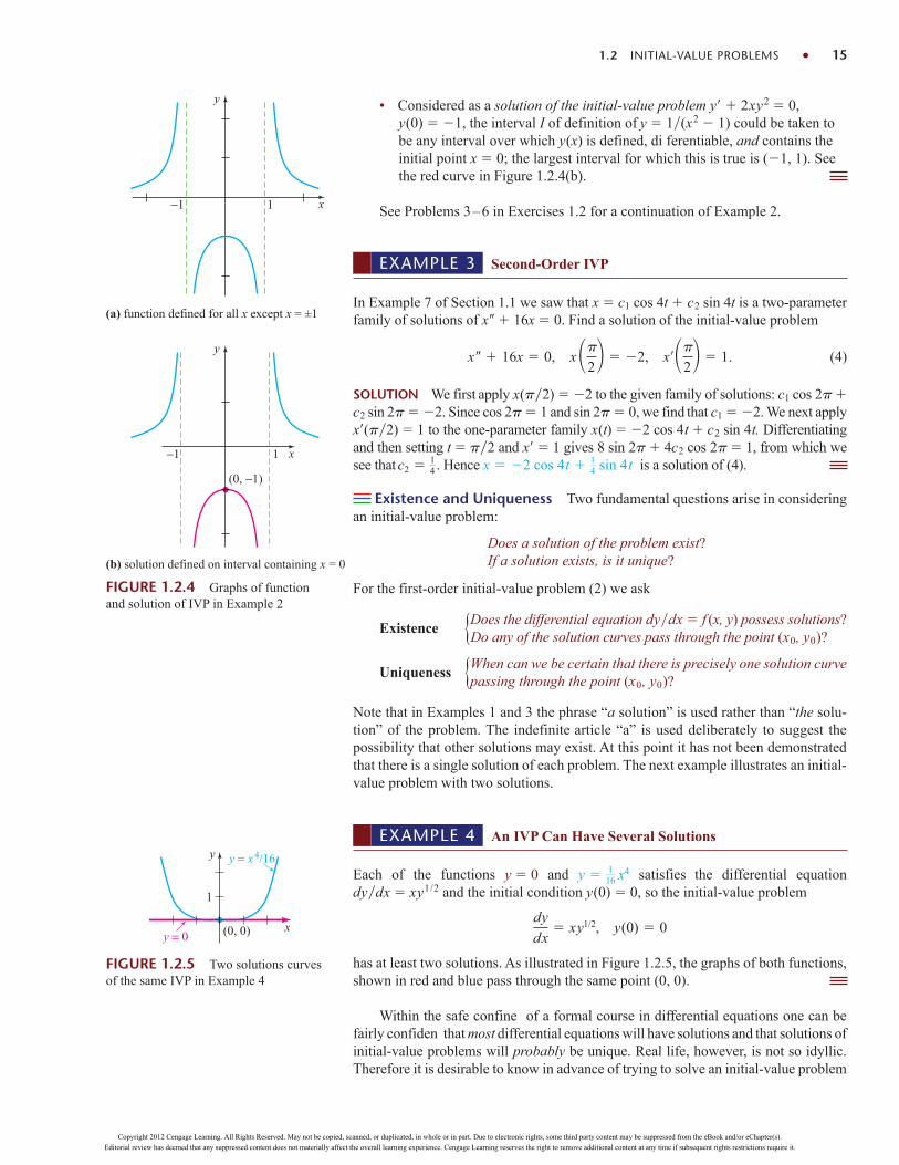
• Considered as a solution of the initial-value problem y 2xy2 0,y(0) 1, the interval I of definition of y 1(x2 1) could be taken tobe any interval over which y(x) is defined, di ferentiable, and contains theinitial point x 0; the largest interval for which this is true is (1, 1). Seethe red curve in Figure 1.2.4(b).
See Problems 3–6 in Exercises 1.2 for a continuation of Example 2.
1.2 INITIAL-VALUE PROBLEMS 15
FIGURE 1.2.4 Graphs of functionand solution of IVP in Example 2
(0, −1)
x
y
1−1
x
y
1−1
(a) function defined for all x except x = ±1
(b) solution defined on interval containing x = 0
y
y = 0
y = x4/16
(0, 0)
1
x
FIGURE 1.2.5 Two solutions curvesof the same IVP in Example 4
EXAMPLE 3 Second-Order IVP
In Example 7 of Section 1.1 we saw that x c1 cos 4t c2 sin 4t is a two-parameterfamily of solutions of x 16x 0. Find a solution of the initial-value problem
(4)
SOLUTION We first apply x(2) 2 to the given family of solutions: c1 cos 2 c2 sin 2 2. Since cos 2 1 and sin 2 0, we find that c1 2. We next applyx(2) 1 to the one-parameter family x(t) 2 cos 4t c2 sin 4t. Differentiatingand then setting t 2 and x 1 gives 8 sin 2 4c2 cos 2 1, from which wesee that . Hence is a solution of (4).
Existence and Uniqueness Two fundamental questions arise in consideringan initial-value problem:
Does a solution of the problem exist?If a solution exists, is it unique?
For the first-order initial-value problem (2) we ask
Existence Does the differential equation dydx f (x, y) possess solutions?Do any of the solution curves pass through the point (x0, y0)?
Uniqueness When can we be certain that there is precisely one solution curvepassing through the point (x0, y0)?
Note that in Examples 1 and 3 the phrase “a solution” is used rather than “the solu-tion” of the problem. The indefinite article “a” is used deliberately to suggest thepossibility that other solutions may exist. At this point it has not been demonstratedthat there is a single solution of each problem. The next example illustrates an initial-value problem with two solutions.
x 2 cos 4t 14 sin 4tc2 1
4
x 16x 0, x
2 2, x
2 1.
EXAMPLE 4 An IVP Can Have Several Solutions
Each of the functions y 0 and satisfies the differential equationdydx xy1/2 and the initial condition y(0) 0, so the initial-value problem
has at least two solutions. As illustrated in Figure 1.2.5, the graphs of both functions,shown in red and blue pass through the same point (0, 0).
Within the safe confine of a formal course in differential equations one can befairly confiden that most differential equations will have solutions and that solutions ofinitial-value problems will probably be unique. Real life, however, is not so idyllic.Therefore it is desirable to know in advance of trying to solve an initial-value problem
dy
dx xy1/2, y(0) 0
y 116 x
4
Copyright 2012 Cengage Learning. All Rights Reserved. May not be copied, scanned, or duplicated, in whole or in part. Due to electronic rights, some third party content may be suppressed from the eBook and/or eChapter(s).
Editorial review has deemed that any suppressed content does not materially affect the overall learning experience. Cengage Learning reserves the right to remove additional content at any time if subsequent rights restrictions require it.

whether a solution exists and, when it does, whether it is the only solution of the prob-lem. Since we are going to consider first-orde differential equations in the next twochapters, we state here without proof a straightforward theorem that gives conditionsthat are sufficien to guarantee the existence and uniqueness of a solution of a first-ordeinitial-value problem of the form given in (2). We shall wait until Chapter 4 to addressthe question of existence and uniqueness of a second-order initial-value problem.
16 CHAPTER 1 INTRODUCTION TO DIFFERENTIAL EQUATIONS
xI0
R
a b
c
d
(x0, y0)
y
FIGURE 1.2.6 Rectangular region R
THEOREM 1.2.1 Existence of a Unique Solution
Let R be a rectangular region in the xy-plane defined by a x b, c y dthat contains the point (x0, y0) in its interior. If f (x, y) and f y are continuouson R, then there exists some interval I0: (x0 h, x0 h), h 0, contained in[a, b], and a unique function y(x), defined on I0, that is a solution of the initial-value problem (2).
The foregoing result is one of the most popular existence and uniqueness theo-rems for first-order differential equations because the criteria of continuity of f (x, y)and fy are relatively easy to check. The geometry of Theorem 1.2.1 is illustratedin Figure 1.2.6.
EXAMPLE 5 Example 4 Revisited
We saw in Example 4 that the differential equation dydx xy1/2 possesses at leasttwo solutions whose graphs pass through (0, 0). Inspection of the functions
shows that they are continuous in the upper half-plane defined by y 0. HenceTheorem 1.2.1 enables us to conclude that through any point (x0, y0), y0 0 in theupper half-plane there is some interval centered at x0 on which the given differentialequation has a unique solution. Thus, for example, even without solving it, we knowthat there exists some interval centered at 2 on which the initial-value problemdydx xy1/2, y(2) 1 has a unique solution.
In Example 1, Theorem 1.2.1 guarantees that there are no other solutions of theinitial-value problems y y, y(0) 3 and y y, y(1) 2 other than y 3ex
and y 2ex1, respectively. This follows from the fact that f (x, y) y andfy 1 are continuous throughout the entire xy-plane. It can be further shown thatthe interval I on which each solution is defined is , ).
Interval of Existence/Uniqueness Suppose y(x) represents a solution ofthe initial-value problem (2). The following three sets on the real x-axis may not bethe same: the domain of the function y(x), the interval I over which the solution y(x)is defined or exists, and the interval I0 of existence and uniqueness. Example 2 ofSection 1.1 illustrated the difference between the domain of a function and theinterval I of definition. Now suppose (x0, y0) is a point in the interior of the rectan-gular region R in Theorem 1.2.1. It turns out that the continuity of the functionf (x, y) on R by itself is sufficient to guarantee the existence of at least one solutionof dydx f (x, y), y(x0) y0, defined on some interval I. The interval I of definition for this initial-value problem is usually taken to be the largest interval contain-ing x0 over which the solution y(x) is defined and differentiable. The interval Idepends on both f (x, y) and the initial condition y(x0) y0. See Problems 31–34 inExercises 1.2. The extra condition of continuity of the first partial derivative fy
f (x, y) xy1/2 andf
y
x
2y1/2
Copyright 2012 Cengage Learning. All Rights Reserved. May not be copied, scanned, or duplicated, in whole or in part. Due to electronic rights, some third party content may be suppressed from the eBook and/or eChapter(s).
Editorial review has deemed that any suppressed content does not materially affect the overall learning experience. Cengage Learning reserves the right to remove additional content at any time if subsequent rights restrictions require it.

1.2 INITIAL-VALUE PROBLEMS 17
on R enables us to say that not only does a solution exist on some interval I0 con-taining x0, but it is the only solution satisfying y(x0) y0. However, Theorem 1.2.1does not give any indication of the sizes of intervals I and I0; the interval I ofdefinition need not be as wide as the region R, and the interval I0 of existence anduniqueness may not be as large as I. The number h 0 that defines the intervalI0: (x0 h, x0 h) could be very small, so it is best to think that the solution y(x)is unique in a local sense —that is, a solution defined near the point (x0, y0). SeeProblem 50 in Exercises 1.2.
REMARKS
(i) The conditions in Theorem 1.2.1 are sufficient but not necessary. This meansthat when f (x, y) and fy are continuous on a rectangular region R, it mustalways follow that a solution of (2) exists and is unique whenever (x0, y0) is apoint interior to R. However, if the conditions stated in the hypothesis ofTheorem 1.2.1 do not hold, then anything could happen: Problem (2) may stillhave a solution and this solution may be unique, or (2) may have several solu-tions, or it may have no solution at all. A rereading of Example 5 reveals that thehypotheses of Theorem 1.2.1 do not hold on the line y 0 for the differentialequation dydx xy1/2, so it is not surprising, as we saw in Example 4 of thissection, that there are two solutions defined on a common interval h x hsatisfying y(0) 0. On the other hand, the hypotheses of Theorem 1.2.1 donot hold on the line y 1 for the differential equation dydx y 1.Nevertheless it can be proved that the solution of the initial-value problemdydx y 1, y(0) 1, is unique. Can you guess this solution?
(ii) You are encouraged to read, think about, work, and then keep in mindProblem 49 in Exercises 1.2.
(iii) Initial conditions are prescribed at a single point x0. But we are also inter-ested in solving differential equations that are subject to conditions specifieon y(x) or its derivative at two different points x0 and x1. Conditions such as
and called boundary conditions. A differential equation together with bound-ary conditions is called a boundary-value problem (BVP). For example,
is a boundary-value problem. See Problems 39–44 in Exercises 1.2.When we start to solve differential equations in Chapter 2 we will solve
only first-order equations and first-order initial-value problems. The mathe-matical description of many problems in science and engineering involvesecond-order IVPs or two-point BVPs. We will examine some of these prob-lems in Chapters 4 and 5.
y ly 0, y(0) 0, y(p) 0
y(1) 0, y(5) 0 or y(p>2) 0, y(p) 1
EXERCISES 1.2 Answers to selected odd-numbered problems begin on page ANS-1.
In Problems 1 and 2, y 1(1 c1ex) is a one-parameterfamily of solutions of the first-order DE y y y2. Find asolution of the first-order IVP consisting of this differentialequation and the given initial condition.
1. 2. y(1) 2
In Problems 3–6, y 1(x2 c) is a one-parameter familyof solutions of the first-order DE y 2xy2 0. Find a
y(0) 13
solution of the first-order IVP consisting of this differentialequation and the given initial condition. Give the largestinterval I over which the solution is defined
3. 4.
5. y(0) 1 6.
In Problems 7–10, x c1 cos t c2 sin t is a two-parameterfamily of solutions of the second-order DE x x 0. Find
y(12) 4
y(2) 12y(2) 1
3
Copyright 2012 Cengage Learning. All Rights Reserved. May not be copied, scanned, or duplicated, in whole or in part. Due to electronic rights, some third party content may be suppressed from the eBook and/or eChapter(s).
Editorial review has deemed that any suppressed content does not materially affect the overall learning experience. Cengage Learning reserves the right to remove additional content at any time if subsequent rights restrictions require it.

a solution of the second-order IVP consisting of this differ-ential equation and the given initial conditions.
7. x(0) 1, x(0) 8
8. x(2) 0, x(2) 1
9.
10.
In Problems 11–14, y c1ex c2ex is a two-parameterfamily of solutions of the second-order DE y y 0. Finda solution of the second-order IVP consisting of this differ-ential equation and the given initial conditions.
11.
12. y(1) 0, y(1) e
13. y(1) 5, y(1) 5
14. y(0) 0, y(0) 0
In Problems 15 and 16 determine by inspection at least twosolutions of the given first-order IV .
15. y 3y2/3, y(0) 0
16. xy 2y, y(0) 0
In Problems 17–24 determine a region of the xy-plane forwhich the given differential equation would have a uniquesolution whose graph passes through a point (x0, y0) in theregion.
17. 18.
19. 20.
21. (4 y2)y x2 22. (1 y3)y x2
23. (x2 y2)y y2 24. (y x)y y x
In Problems 25–28 determine whether Theorem 1.2.1 guar-antees that the differential equation pos-sesses a unique solution through the given point.
25. (1, 4) 26. (5, 3)
27. (2, 3) 28. (1, 1)
29. (a) By inspection find a one-parameter family of solu-tions of the differential equation xy y. Verify thateach member of the family is a solution of theinitial-value problem xy y, y(0) 0.
(b) Explain part (a) by determining a region R in thexy-plane for which the differential equation xy ywould have a unique solution through a point (x0, y0)in R.
y 1y2 9
dy
dx y xx
dy
dx y
dy
dx 1xy
dy
dx y2/3
y(0) 2y(0) 1,
x(>4) 12, x(>4) 212
x(>6) 12, x(>6) 0
18 CHAPTER 1 INTRODUCTION TO DIFFERENTIAL EQUATIONS
(c) Verify that the piecewise-defined functio
satisfies the condition y(0) 0. Determine whetherthis function is also a solution of the initial-valueproblem in part (a).
30. (a) Verify that y tan (x c) is a one-parameter familyof solutions of the differential equation y 1 y2.
(b) Since f (x, y) 1 y2 and fy 2y are continu-ous everywhere, the region R in Theorem 1.2.1 canbe taken to be the entire xy-plane. Use the family ofsolutions in part (a) to find an explicit solution ofthe first-order initial-value problem y 1 y2,y(0) 0. Even though x0 0 is in the interval(2, 2), explain why the solution is not defined onthis interval.
(c) Determine the largest interval I of definition for thesolution of the initial-value problem in part (b).
31. (a) Verify that y 1(x c) is a one-parameterfamily of solutions of the differential equation y y2.
(b) Since f (x, y) y2 and fy 2y are continuouseverywhere, the region R in Theorem 1.2.1 can betaken to be the entire xy-plane. Find a solution fromthe family in part (a) that satisfies y(0) 1. Thenfind a solution from the family in part (a) thatsatisfies y(0) 1. Determine the largest interval Iof definition for the solution of each initial-valueproblem.
(c) Determine the largest interval I of definition for thesolution of the first-order initial-value problemy y2, y(0) 0. [Hint: The solution is not a mem-ber of the family of solutions in part (a).]
32. (a) Show that a solution from the family in part (a)of Problem 31 that satisfies y y2, y(1) 1, isy 1(2 x).
(b) Then show that a solution from the family in part (a)of Problem 31 that satisfies y y2, y(3) 1, isy 1(2 x).
(c) Are the solutions in parts (a) and (b) the same?
33. (a) Verify that 3x2 y2 c is a one-parameter fam-ily of solutions of the differential equation y dydx 3x.
(b) By hand, sketch the graph of the implicit solution3x2 y2 3. Find all explicit solutions y (x) ofthe DE in part (a) defined by this relation. Give theinterval I of definition of each explicit solution
(c) The point (2, 3) is on the graph of 3x2 y2 3,but which of the explicit solutions in part (b) satis-fies y(2) 3?
34. (a) Use the family of solutions in part (a) of Problem 33to find an implicit solution of the initial-value
y 0, x 0
x, x 0
Copyright 2012 Cengage Learning. All Rights Reserved. May not be copied, scanned, or duplicated, in whole or in part. Due to electronic rights, some third party content may be suppressed from the eBook and/or eChapter(s).
Editorial review has deemed that any suppressed content does not materially affect the overall learning experience. Cengage Learning reserves the right to remove additional content at any time if subsequent rights restrictions require it.

1.2 INITIAL-VALUE PROBLEMS 19
FIGURE 1.2.7 Graph for Problem 35
y
x
5
−5
5
In Problems 39–44, is a two-parameter family of solutions of the second-order DE
If possible, find a solution of the differentialequation that satisfies the given side conditions. The condi-tions specified at two different points are called boundaryconditions.
39. 40.
41. 42.
43. 44.
Discussion Problems
In Problems 45 and 46 use Problem 51 in Exercises 1.1 and(2) and (3) of this section.
45. Find a function y f (x) whose graph at each point (x, y)has the slope given by 8e2x 6x and has the y-intercept (0, 9).
46. Find a function y f (x) whose second derivative isy 12x 2 at each point (x, y) on its graph andy x 5 is tangent to the graph at the point corre-sponding to x 1.
47. Consider the initial-value problem y x 2y,. Determine which of the two curves shown
in Figure 1.2.11 is the only plausible solution curve.Explain your reasoning.
y(0) 12
y(p>2) 1, y(p) 0y(0) 0, y(p) 2
y(0) 1, y(p) 5y(0) 0, y(p>6) 0
y(0) 0, y(p) 0y(0) 0, y(p>4) 3
y 4y 0.
y c1 cos 2x c2 sin 2x
FIGURE 1.2.10 Graph for Problem 38
y
x
5
−5
5
36.
37.
38.
FIGURE 1.2.8 Graph for Problem 36
FIGURE 1.2.9 Graph for Problem 37
y
x
5
−5
5
y
x
5
−5
5
FIGURE 1.2.11 Graphs for Problem 47
(0, )12
1
1 x
y
problem y dydx 3x, y(2) 4. Then, by hand,sketch the graph of the explicit solution of thisproblem and give its interval I of definition
(b) Are there any explicit solutions of y dydx 3x thatpass through the origin?
In Problems 35–38 the graph of a member of a familyof solutions of a second-order differential equation d2ydx2 f (x, y, y) is given. Match the solution curve withat least one pair of the following initial conditions.
(a) y(1) 1, y(1) 2
(b) y(1) 0, y(1) 4
(c) y(1) 1, y(1) 2
(d) y(0) 1, y(0) 2
(e) y(0) 1, y(0) 0
(f ) y(0) 4, y(0) 2
35.
48. Determine a plausible value of x0 for which thegraph of the solution of the initial-value problem y 2y 3x 6, y(x0) 0 is tangent to the x-axis at(x0, 0). Explain your reasoning.
Copyright 2012 Cengage Learning. All Rights Reserved. May not be copied, scanned, or duplicated, in whole or in part. Due to electronic rights, some third party content may be suppressed from the eBook and/or eChapter(s).
Editorial review has deemed that any suppressed content does not materially affect the overall learning experience. Cengage Learning reserves the right to remove additional content at any time if subsequent rights restrictions require it.
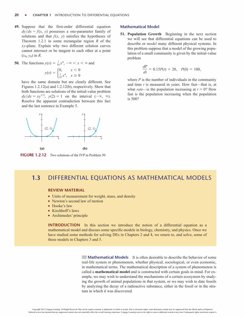
20 CHAPTER 1 INTRODUCTION TO DIFFERENTIAL EQUATIONS
49. Suppose that the first-order differential equation dydx f (x, y) possesses a one-parameter family ofsolutions and that f (x, y) satisfies the hypotheses ofTheorem 1.2.1 in some rectangular region R of the xy-plane. Explain why two different solution curvescannot intersect or be tangent to each other at a point(x0, y0) in R.
50. The functions and
have the same domain but are clearly different. SeeFigures 1.2.12(a) and 1.2.12(b), respectively. Show thatboth functions are solutions of the initial-value problemdydx xy1/2, y(2) 1 on the interval (, ).Resolve the apparent contradiction between this factand the last sentence in Example 5.
y(x) 0,116 x
4,
x 0
x 0
y(x) 116 x
4, x
Mathematical Model
51. Population Growth Beginning in the next sectionwe will see that differential equations can be used todescribe or model many different physical systems. Inthis problem suppose that a model of the growing popu-lation of a small community is given by the initial-valueproblem
where P is the number of individuals in the communityand time t is measured in years. How fast—that is, atwhat rate—is the population increasing at t 0? Howfast is the population increasing when the populationis 500?
dP
dt 0.15P(t) 20, P(0) 100,
FIGURE 1.2.12 Two solutions of the IVP in Problem 50
(a)
(2, 1)
y
x
(b)
(2, 1)
y
x
Mathematical Models It is often desirable to describe the behavior of somereal-life system or phenomenon, whether physical, sociological, or even economic,in mathematical terms. The mathematical description of a system of phenomenon iscalled a mathematical model and is constructed with certain goals in mind. For ex-ample, we may wish to understand the mechanisms of a certain ecosystem by study-ing the growth of animal populations in that system, or we may wish to date fossilsby analyzing the decay of a radioactive substance, either in the fossil or in the stra-tum in which it was discovered.
DIFFERENTIAL EQUATIONS AS MATHEMATICAL MODELS
REVIEW MATERIAL Units of measurement for weight, mass, and density Newton’s second law of motion Hooke’s law Kirchhoff’s laws Archimedes’ principle
INTRODUCTION In this section we introduce the notion of a differential equation as amathematical model and discuss some specific models in biology, chemistry, and physics. Once wehave studied some methods for solving DEs in Chapters 2 and 4, we return to, and solve, some ofthese models in Chapters 3 and 5.
1.3
Copyright 2012 Cengage Learning. All Rights Reserved. May not be copied, scanned, or duplicated, in whole or in part. Due to electronic rights, some third party content may be suppressed from the eBook and/or eChapter(s).
Editorial review has deemed that any suppressed content does not materially affect the overall learning experience. Cengage Learning reserves the right to remove additional content at any time if subsequent rights restrictions require it.

Construction of a mathematical model of a system starts with
(i) identification of the variables that are responsible for changing thesystem. We may choose not to incorporate all these variables into themodel at first. In this step we are specifying the level of resolution ofthe model.
Next
(ii) we make a set of reasonable assumptions, or hypotheses, about thesystem we are trying to describe. These assumptions will also includeany empirical laws that may be applicable to the system.
For some purposes it may be perfectly within reason to be content with low-resolution models. For example, you may already be aware that in beginningphysics courses, the retarding force of air friction is sometimes ignored in modelingthe motion of a body falling near the surface of the Earth, but if you are a scientistwhose job it is to accurately predict the flight path of a long-range projectile,you have to take into account air resistance and other factors such as the curvatureof the Earth.
Since the assumptions made about a system frequently involve a rate of changeof one or more of the variables, the mathematical depiction of all these assumptionsmay be one or more equations involving derivatives. In other words, the mathemat-ical model may be a differential equation or a system of differential equations.
Once we have formulated a mathematical model that is either a differentialequation or a system of differential equations, we are faced with the not insignificanproblem of trying to solve it. If we can solve it, then we deem the model to be reason-able if its solution is consistent with either experimental data or known facts aboutthe behavior of the system. But if the predictions produced by the solution are poor,we can either increase the level of resolution of the model or make alternative as-sumptions about the mechanisms for change in the system. The steps of the model-ing process are then repeated, as shown in the diagram in Figure 1.3.1.
1.3 DIFFERENTIAL EQUATIONS AS MATHEMATICAL MODELS 21
Express assumptionsin terms of DEs
Display predictionsof model
(e.g., graphically)
Solve the DEs
If necessary,alter assumptions
or increase resolutionof model
Assumptionsand hypotheses
Mathematicalformulation
Obtainsolutions
Check modelpredictions with
known facts
FIGURE 1.3.1 Steps in the modeling process with differential equations
Of course, by increasing the resolution, we add to the complexity of the mathemati-cal model and increase the likelihood that we cannot obtain an explicit solution.
A mathematical model of a physical system will often involve the variable time t.A solution of the model then gives the state of the system; in other words, the valuesof the dependent variable (or variables) for appropriate values of t describe the systemin the past, present, and future.
Population Dynamics One of the earliest attempts to model human pop-ulation growth by means of mathematics was by the English clergyman and econo-mist Thomas Malthus in 1798. Basically, the idea behind the Malthusian model is theassumption that the rate at which the population of a country grows at a certain time is
Copyright 2012 Cengage Learning. All Rights Reserved. May not be copied, scanned, or duplicated, in whole or in part. Due to electronic rights, some third party content may be suppressed from the eBook and/or eChapter(s).
Editorial review has deemed that any suppressed content does not materially affect the overall learning experience. Cengage Learning reserves the right to remove additional content at any time if subsequent rights restrictions require it.

proportional* to the total population of the country at that time. In other words, the morepeople there are at time t, the more there are going to be in the future. In mathematicalterms, if P(t) denotes the total population at time t, then this assumption can beexpressed as
, (1)
where k is a constant of proportionality. This simple model, which fails to take intoaccount many factors that can influence human populations to either grow or decline(immigration and emigration, for example), nevertheless turned out to be fairly accu-rate in predicting the population of the United States during the years 1790–1860.Populations that grow at a rate described by (1) are rare; nevertheless, (1) is still usedto model growth of small populations over short intervals of time (bacteria growingin a petri dish, for example).
Radioactive Decay The nucleus of an atom consists of combinations of protonsand neutrons. Many of these combinations of protons and neutrons are unstable—thatis, the atoms decay or transmute into atoms of another substance. Such nuclei aresaid to be radioactive. For example, over time the highly radioactive radium, Ra-226,transmutes into the radioactive gas radon, Rn-222. To model the phenomenon ofradioactive decay, it is assumed that the rate dAdt at which the nuclei of a sub-stance decay is proportional to the amount (more precisely, the number of nuclei)A(t) of the substance remaining at time t:
. (2)
Of course, equations (1) and (2) are exactly the same; the difference is only in the in-terpretation of the symbols and the constants of proportionality. For growth, as weexpect in (1), k 0, and for decay, as in (2), k 0.
The model (1) for growth can also be seen as the equation dSdt rS, whichdescribes the growth of capital S when an annual rate of interest r is compoundedcontinuously. The model (2) for decay also occurs in biological applications such asdetermining the half-life of a drug—the time that it takes for 50% of a drug to beeliminated from a body by excretion or metabolism. In chemistry the decay model(2) appears in the mathematical description of a first-order chemical reaction. Thepoint is this:
A single differential equation can serve as a mathematical model for manydifferent phenomena.
Mathematical models are often accompanied by certain side conditions. For ex-ample, in (1) and (2) we would expect to know, in turn, the initial population P0 andthe initial amount of radioactive substance A0 on hand. If the initial point in time istaken to be t 0, then we know that P(0) P0 and A(0) A0. In other words, amathematical model can consist of either an initial-value problem or, as we shall seelater on in Section 5.2, a boundary-value problem.
Newton’s Law of Cooling/Warming According to Newton’s empiricallaw of cooling/warming, the rate at which the temperature of a body changes isproportional to the difference between the temperature of the body and the temper-ature of the surrounding medium, the so-called ambient temperature. If T(t) repre-sents the temperature of a body at time t, Tm the temperature of the surrounding
dA
dt A or
dA
dt kA
dP
dt P or
dP
dt kP
22 CHAPTER 1 INTRODUCTION TO DIFFERENTIAL EQUATIONS
*If two quantities u and v are proportional, we write u v. This means that one quantity is a constantmultiple of the other: u kv.
Copyright 2012 Cengage Learning. All Rights Reserved. May not be copied, scanned, or duplicated, in whole or in part. Due to electronic rights, some third party content may be suppressed from the eBook and/or eChapter(s).
Editorial review has deemed that any suppressed content does not materially affect the overall learning experience. Cengage Learning reserves the right to remove additional content at any time if subsequent rights restrictions require it.
medium, and dTdt the rate at which the temperature of the body changes, thenNewton’s law of cooling/warming translates into the mathematical statement
, (3)
where k is a constant of proportionality. In either case, cooling or warming, if Tm is aconstant, it stands to reason that k 0.
Spread of a Disease A contagious disease—for example, a flu virus—isspread throughout a community by people coming into contact with other people. Letx(t) denote the number of people who have contracted the disease and y(t) denote thenumber of people who have not yet been exposed. It seems reasonable to assume thatthe rate dxdt at which the disease spreads is proportional to the number of encoun-ters, or interactions, between these two groups of people. If we assume that the num-ber of interactions is jointly proportional to x(t) and y(t)—that is, proportional to theproduct xy—then
, (4)
where k is the usual constant of proportionality. Suppose a small community has afixed population of n people. If one infected person is introduced into this commu-nity, then it could be argued that x(t) and y(t) are related by x y n 1. Usingthis last equation to eliminate y in (4) gives us the model
. (5)
An obvious initial condition accompanying equation (5) is x(0) 1.
Chemical Reactions The disintegration of a radioactive substance, governedby the differential equation (1), is said to be a first-orde reaction. In chemistrya few reactions follow this same empirical law: If the molecules of substance Adecompose into smaller molecules, it is a natural assumption that the rate at whichthis decomposition takes place is proportional to the amount of the first substancethat has not undergone conversion; that is, if X(t) is the amount of substance Aremaining at any time, then dXdt kX, where k is a negative constant since X isdecreasing. An example of a first-order chemical reaction is the conversion of t-butylchloride, (CH3)3CCl, into t-butyl alcohol, (CH3)3COH:
Only the concentration of the t-butyl chloride controls the rate of reaction. But in thereaction
one molecule of sodium hydroxide, NaOH, is consumed for every molecule ofmethyl chloride, CH3Cl, thus forming one molecule of methyl alcohol, CH3OH, andone molecule of sodium chloride, NaCl. In this case the rate at which the reactionproceeds is proportional to the product of the remaining concentrations of CH3Cl andNaOH. To describe this second reaction in general, let us suppose one molecule of asubstance A combines with one molecule of a substance B to form one molecule of asubstance C. If X denotes the amount of chemical C formed at time t and if and are, in turn, the amounts of the two chemicals A and B at t 0 (the initial amounts),then the instantaneous amounts of A and B not converted to chemical C are Xand X, respectively. Hence the rate of formation of C is given by
, (6)
where k is a constant of proportionality. A reaction whose model is equation (6) issaid to be a second-order reaction.
dX
dt k( X)( X)
CH3Cl NaOH : CH3OH NaCl
(CH3)3CCl NaOH : (CH3)3COH NaCl.
dx
dt kx(n 1 x)
dx
dt kxy
dT
dt T Tm or
dT
dt k(T Tm)
1.3 DIFFERENTIAL EQUATIONS AS MATHEMATICAL MODELS 23
Copyright 2012 Cengage Learning. All Rights Reserved. May not be copied, scanned, or duplicated, in whole or in part. Due to electronic rights, some third party content may be suppressed from the eBook and/or eChapter(s).
Editorial review has deemed that any suppressed content does not materially affect the overall learning experience. Cengage Learning reserves the right to remove additional content at any time if subsequent rights restrictions require it.

Mixtures The mixing of two salt solutions of differing concentrations givesrise to a first-order differential equation for the amount of salt contained in the mix-ture. Let us suppose that a large mixing tank initially holds 300 gallons of brine (thatis, water in which a certain number of pounds of salt has been dissolved). Anotherbrine solution is pumped into the large tank at a rate of 3 gallons per minute; theconcentration of the salt in this inflow is 2 pounds per gallon. When the solution inthe tank is well stirred, it is pumped out at the same rate as the entering solution. SeeFigure 1.3.2. If A(t) denotes the amount of salt (measured in pounds) in the tank attime t, then the rate at which A(t) changes is a net rate:
. (7)
The input rate Rin at which salt enters the tank is the product of the inflow concentra-tion of salt and the inflow rate of fluid. Note that Rin is measured in pounds perminute:
Now, since the solution is being pumped out of the tank at the same rate that it ispumped in, the number of gallons of brine in the tank at time t is a constant 300 gal-lons. Hence the concentration of the salt in the tank as well as in the outflow isc(t) A(t)300 lb/gal, so the output rate Rout of salt is
The net rate (7) then becomes
(8)
If rin and rout denote general input and output rates of the brine solutions,* thenthere are three possibilities: rin rout, rin rout, and rin rout. In the analysis lead-ing to (8) we have assumed that rin rout. In the latter two cases the number of gal-lons of brine in the tank is either increasing (rin rout) or decreasing (rin rout) atthe net rate rin rout. See Problems 10–12 in Exercises 1.3.
Draining a Tank In hydrodynamics, Torricelli’s law states that the speed v ofefflux of water though a sharp-edged hole at the bottom of a tank filled to a depth his the same as the speed that a body (in this case a drop of water) would acquire infalling freely from a height h—that is, , where g is the acceleration due togravity. This last expression comes from equating the kinetic energy with thepotential energy mgh and solving for v. Suppose a tank filled with water is allowed todrain through a hole under the influence of gravity. We would like to fin the depth hof water remaining in the tank at time t. Consider the tank shown in Figure 1.3.3. Ifthe area of the hole is Ah (in ft2) and the speed of the water leaving the tank is
(in ft/s), then the volume of water leaving the tank per second is (in ft3/s). Thus if V(t) denotes the volume of water in the tank at time t, then
, (9)dV
dt Ah12gh
Ah12ghv 12gh
12mv2
v 12gh
dA
dt 6
A
100or
dA
dt
1
100 A 6.
Rout ( lb/gal) (3 gal/min) lb/min.A(t)––––300
A(t)––––100
concentrationof salt
in outflooutput rate
of brineoutput rate
of salt
concentrationof salt
in infloinput rateof brine
input rateof salt
Rin (2 lb/gal) (3 gal/min) (6 lb/min).
dA
dt input rate
of salt output rate
of salt Rin Rout
24 CHAPTER 1 INTRODUCTION TO DIFFERENTIAL EQUATIONS
input rate of brine3 gal/min
output rate of brine3 gal/min
constant300 gal
FIGURE 1.3.2 Mixing tank
h
Aw
Ah
FIGURE 1.3.3 Draining tank
*Don’t confuse these symbols with Rin and Rout, which are input and output rates of salt.
Copyright 2012 Cengage Learning. All Rights Reserved. May not be copied, scanned, or duplicated, in whole or in part. Due to electronic rights, some third party content may be suppressed from the eBook and/or eChapter(s).
Editorial review has deemed that any suppressed content does not materially affect the overall learning experience. Cengage Learning reserves the right to remove additional content at any time if subsequent rights restrictions require it.

where the minus sign indicates that V is decreasing. Note here that we are ignoringthe possibility of friction at the hole that might cause a reduction of the rate of flothere. Now if the tank is such that the volume of water in it at time t can be writtenV(t) Awh, where Aw (in ft2) is the constant area of the upper surface of the water(see Figure 1.3.3), then dVdt Aw dhdt. Substituting this last expression into (9)gives us the desired differential equation for the height of the water at time t:
. (10)
It is interesting to note that (10) remains valid even when Aw is not constant. In thiscase we must express the upper surface area of the water as a function of h—that is,Aw A(h). See Problem 14 in Exercises 1.3.
Series Circuits Consider the single-loop LRC-series circuit shown in Fig-ure 1.3.4(a), containing an inductor, resistor, and capacitor. The current in a circuitafter a switch is closed is denoted by i(t); the charge on a capacitor at time t is de-noted by q(t). The letters L, R, and C are known as inductance, resistance, and capac-itance, respectively, and are generally constants. Now according to Kirchhoff’ssecond law, the impressed voltage E(t) on a closed loop must equal the sum of thevoltage drops in the loop. Figure 1.3.4(b) shows the symbols and the formulas for therespective voltage drops across an inductor, a capacitor, and a resistor. Since currenti(t) is related to charge q(t) on the capacitor by i dqdt, adding the three voltages
inductor resistor capacitor
and equating the sum to the impressed voltage yields a second-order differentialequation
(11)
We will examine a differential equation analogous to (11) in great detail inSection 5.1.
Falling Bodies To construct a mathematical model of the motion of a bodymoving in a force field, one often starts with the laws of motion formulated by theEnglish mathematician Isaac Newton (1643–1727). Recall from elementary physicsthat Newton’s first law of motion states that a body either will remain at rest or willcontinue to move with a constant velocity unless acted on by an external force. Ineach case this is equivalent to saying that when the sum of the forces —that is, the net or resultant force—acting on the body is zero, then the accelerationa of the body is zero. Newton’s second law of motion indicates that when the netforce acting on a body is not zero, then the net force is proportional to its accelera-tion a or, more precisely, F ma, where m is the mass of the body.
Now suppose a rock is tossed upward from the roof of a building as illustratedin Figure 1.3.5. What is the position s(t) of the rock relative to the ground at time t?The acceleration of the rock is the second derivative d 2sdt2. If we assume that theupward direction is positive and that no force acts on the rock other than the force ofgravity, then Newton’s second law gives
. (12)
In other words, the net force is simply the weight F F1 W of the rock near thesurface of the Earth. Recall that the magnitude of the weight is W mg, where m is
m d 2s
dt2 mg ord 2s
dt2 g
F Fk
L d 2q
dt2 R dq
dt
1
C q E(t).
L di
dt L
d 2q
dt2 , iR R dq
dt, and
1
C q
dh
dt
Ah
Aw
12gh
1.3 DIFFERENTIAL EQUATIONS AS MATHEMATICAL MODELS 25
(a)
(b)
E(t)L
C
R
(a) LRC-series circuit
(b)
L
R
Inductorinductance L: henries (h)
voltage drop across: Ldidt
i
Capacitorcapacitance C: farads (f)
voltage drop across:1C
i
Resistorresistance R: ohms (Ω)voltage drop across: iR
i
q
C
FIGURE 1.3.4 Symbols, units, andvoltages. Current i(t) and charge q(t) aremeasured in amperes (A) and coulombs(C), respectively
ground
building
rock
s(t)s0
v0
FIGURE 1.3.5 Position of rockmeasured from ground level
Copyright 2012 Cengage Learning. All Rights Reserved. May not be copied, scanned, or duplicated, in whole or in part. Due to electronic rights, some third party content may be suppressed from the eBook and/or eChapter(s).
Editorial review has deemed that any suppressed content does not materially affect the overall learning experience. Cengage Learning reserves the right to remove additional content at any time if subsequent rights restrictions require it.

the mass of the body and g is the acceleration due to gravity. The minus sign in (12) isused because the weight of the rock is a force directed downward, which is oppositeto the positive direction. If the height of the building is s0 and the initial velocity of therock is v0, then s is determined from the second-order initial-value problem
. (13)
Although we have not been stressing solutions of the equations we have con-structed, note that (13) can be solved by integrating the constant g twice withrespect to t. The initial conditions determine the two constants of integration.From elementary physics you might recognize the solution of (13) as the formula
Falling Bodies and Air Resistance Before the famous experiment by theItalian mathematician and physicist Galileo Galilei (1564–1642) from the leaningtower of Pisa, it was generally believed that heavier objects in free fall, such as a can-nonball, fell with a greater acceleration than lighter objects, such as a feather.Obviously, a cannonball and a feather when dropped simultaneously from the sameheight do fall at different rates, but it is not because a cannonball is heavier. The dif-ference in rates is due to air resistance. The resistive force of air was ignored in themodel given in (13). Under some circumstances a falling body of mass m, such as afeather with low density and irregular shape, encounters air resistance proportionalto its instantaneous velocity v. If we take, in this circumstance, the positive directionto be oriented downward, then the net force acting on the mass is given by F F1 F2 mg kv, where the weight F1 mg of the body is force acting in the positivedirection and air resistance F2 kv is a force, called viscous damping, acting in theopposite or upward direction. See Figure 1.3.6. Now since v is related to accelerationa by a dvdt, Newton’s second law becomes F ma m dvdt. By equating thenet force to this form of Newton’s second law, we obtain a first-order differentialequation for the velocity v(t) of the body at time t,
. (14)
Here k is a positive constant of proportionality. If s(t) is the distance the body falls intime t from its initial point of release, then v dsdt and a dvdt d2sdt2. Interms of s, (14) is a second-order differential equation
(15)
Suspended Cables Suppose a flexible cable, wire, or heavy rope is sus-pended between two vertical supports. Physical examples of this could be one of thetwo cables supporting the roadbed of a suspension bridge as shown in Figure 1.3.7(a)or a long telephone wire strung between two posts as shown in Figure 1.3.7(b). Ourgoal is to construct a mathematical model that describes the shape that such a cableassumes.
To begin, let’s agree to examine only a portion or element of the cable betweenits lowest point P1 and any arbitrary point P2. As drawn in blue in Figure 1.3.8, thiselement of the cable is the curve in a rectangular coordinate system with y-axis cho-sen to pass through the lowest point P1 on the curve and the x-axis chosen a unitsbelow P1. Three forces are acting on the cable: the tensions T1 and T2 in the cablethat are tangent to the cable at P1 and P2, respectively, and the portion W of the totalvertical load between the points P1 and P2. Let T1 T1, T2 T2, and W W denote the magnitudes of these vectors. Now the tension T2 resolvesinto horizontal and vertical components (scalar quantities) T2 cos and T2 sin .
m d 2s
dt 2 mg k ds
dtor m
d 2s
dt 2 k ds
dt mg.
m dv
dt mg kv
s(t) 12gt2 v0t s0.
d 2s
dt 2 g, s(0) s0, s(0) v0
26 CHAPTER 1 INTRODUCTION TO DIFFERENTIAL EQUATIONS
positivedirection
air resistance
gravity
kv
mg
FIGURE 1.3.6 Falling body of mass m
(a) suspension bridge cable
(b) telephone wires
FIGURE 1.3.7 Cables suspendedbetween vertical supports
FIGURE 1.3.8 Element of cable
coswire T2 θθ
sinT2
T2
P2
T1
W
P1
θ
y
x(x, 0)
(0, a)
Copyright 2012 Cengage Learning. All Rights Reserved. May not be copied, scanned, or duplicated, in whole or in part. Due to electronic rights, some third party content may be suppressed from the eBook and/or eChapter(s).
Editorial review has deemed that any suppressed content does not materially affect the overall learning experience. Cengage Learning reserves the right to remove additional content at any time if subsequent rights restrictions require it.

Because of static equilibrium we can write
By dividing the last equation by the first, we eliminate T2 and get tan WT1. Butbecause dydx tan , we arrive at
(16)
This simple first-order differential equation serves as a model for both the shape of aflexible wire such as a telephone wire hanging under its own weight and the shape ofthe cables that support the roadbed of a suspension bridge. We will come back toequation (16) in Exercises 2.2 and Section 5.3.
What Lies Ahead Throughout this text you will see three different types ofapproaches to, or analyses of, differential equations. Over the centuries differentialequations would often spring from the efforts of a scientist or engineer to describesome physical phenomenon or to translate an empirical or experimental law intomathematical terms. As a consequence, a scientist, engineer, or mathematicianwould often spend many years of his or her life trying to fin the solutions of a DE.With a solution in hand, the study of its properties then followed. This quest for so-lutions is called by some the analytical approach to differential equations. Once theyrealized that explicit solutions are at best difficul to obtain and at worst impossibleto obtain, mathematicians learned that a differential equation itself could be a font ofvaluable information. It is possible, in some instances, to glean directly from the dif-ferential equation answers to questions such as Does the DE actually have solutions?If a solution of the DE exists and satisfie an initial condition, is it the only such so-lution? What are some of the properties of the unknown solutions? What can we sayabout the geometry of the solution curves? Such an approach is qualitative analysis.Finally, if a differential equation cannot be solved by analytical methods, yet wecan prove that a solution exists, the next logical query is Can we somehow approxi-mate the values of an unknown solution? Here we enter the realm of numericalanalysis. An affirmativ answer to the last question stems from the fact that a differ-ential equation can be used as a cornerstone for constructing very accurate approxi-mation algorithms. In Chapter 2 we start with qualitative considerations of firstorder ODEs, then examine analytical stratagems for solving some special first-ordeequations, and conclude with an introduction to an elementary numerical method.See Figure 1.3.9.
dy
dx
W
T1
.
T1 T2 cos and W T2 sin .
1.3 DIFFERENTIAL EQUATIONS AS MATHEMATICAL MODELS 27
(a) analytical (b) qualitative (c) numerical
y'=f(y)
FIGURE 1.3.9 Different approaches to the study of differential equations
Copyright 2012 Cengage Learning. All Rights Reserved. May not be copied, scanned, or duplicated, in whole or in part. Due to electronic rights, some third party content may be suppressed from the eBook and/or eChapter(s).
Editorial review has deemed that any suppressed content does not materially affect the overall learning experience. Cengage Learning reserves the right to remove additional content at any time if subsequent rights restrictions require it.
28 CHAPTER 1 INTRODUCTION TO DIFFERENTIAL EQUATIONS
REMARKS
Each example in this section has described a dynamical system—a system thatchanges or evolves with the flow of time t. Since the study of dynamicalsystems is a branch of mathematics currently in vogue, we shall occasionallyrelate the terminology of that field to the discussion at hand
In more precise terms, a dynamical system consists of a set of time-dependent variables, called state variables, together with a rule that enablesus to determine (without ambiguity) the state of the system (this may be a past,present, or future state) in terms of a state prescribed at some time t0. Dynamicalsystems are classifie as either discrete-time systems or continuous-time systems.In this course we shall be concerned only with continuous-time systems—systems in which all variables are defined over a continuous range of time. Therule, or mathematical model, in a continuous-time dynamical system is a differ-ential equation or a system of differential equations. The state of the systemat a time t is the value of the state variables at that time; the specified state ofthe system at a time t0 is simply the initial conditions that accompany the math-ematical model. The solution of the initial-value problem is referred to as theresponse of the system. For example, in the case of radioactive decay, the ruleis dAdt kA. Now if the quantity of a radioactive substance at some time t0 isknown, say A(t0) A0, then by solving the rule we find that the response of thesystem for t t0 is (see Section 3.1). The response A(t) is thesingle state variable for this system. In the case of the rock tossed from the roofof a building, the response of the system—the solution of the differentialequation d2sdt2 g, subject to the initial state s(0) s0, s(0) v0 , is thefunction , where T represents the timewhen the rock hits the ground. The state variables are s(t) and s(t), whichare the vertical position of the rock above ground and its velocity at time t,respectively. The acceleration s(t) is not a state variable, since we have to knowonly any initial position and initial velocity at a time t0 to uniquely determinethe rock’s position s(t) and velocity s(t) v(t) for any time in the interval t0 t T. The acceleration s(t) a(t) is, of course, given by the differentialequation s(t) g, 0 t T.
One last point: Not every system studied in this text is a dynamical system.We shall also examine some static systems in which the model is a differentialequation.
s(t) 12gt2 v0t s0, 0 t T
A(t) A0e(t t0)
EXERCISES 1.3 Answers to selected odd-numbered problems begin on page ANS-1.
Population Dynamics
1. Under the same assumptions that underlie the model in(1), determine a differential equation for the populationP(t) of a country when individuals are allowed toimmigrate into the country at a constant rate r 0.What is the differential equation for the population P(t)of the country when individuals are allowed to emigratefrom the country at a constant rate r 0?
2. The population model given in (1) fails to take deathinto consideration; the growth rate equals the birth rate.In another model of a changing population of a commu-nity it is assumed that the rate at which the populationchanges is a net rate—that is, the difference between
the rate of births and the rate of deaths in the commu-nity. Determine a model for the population P(t) if boththe birth rate and the death rate are proportional to thepopulation present at time t 0.
3. Using the concept of net rate introduced in Problem 2,determine a model for a population P(t) if the birth rateis proportional to the population present at time t but thedeath rate is proportional to the square of the populationpresent at time t.
4. Modify the model in Problem 3 for net rate at whichthe population P(t) of a certain kind of fish changes byalso assuming that the fish are harvested at a constantrate h 0.
Copyright 2012 Cengage Learning. All Rights Reserved. May not be copied, scanned, or duplicated, in whole or in part. Due to electronic rights, some third party content may be suppressed from the eBook and/or eChapter(s).
Editorial review has deemed that any suppressed content does not materially affect the overall learning experience. Cengage Learning reserves the right to remove additional content at any time if subsequent rights restrictions require it.

1.3 DIFFERENTIAL EQUATIONS AS MATHEMATICAL MODELS 29
Newton’s Law of Cooling/Warming
5. A cup of coffee cools according to Newton’s law ofcooling (3). Use data from the graph of the temperatureT(t) in Figure 1.3.10 to estimate the constants Tm, T0,and k in a model of the form of a first-order initial-valueproblem: dTdt k(T Tm), T(0) T0.
number of people x(t) who have adopted the innovationat time t if it is assumed that the rate at which the innova-tions spread through the community is jointly propor-tional to the number of people who have adopted it andthe number of people who have not adopted it.
Mixtures
9. Suppose that a large mixing tank initially holds 300 gal-lons of water in which 50 pounds of salt have been dis-solved. Pure water is pumped into the tank at a rate of3 gal/min, and when the solution is well stirred, it isthen pumped out at the same rate. Determine a differen-tial equation for the amount of salt A(t) in the tank attime t 0. What is A(0)?
10. Suppose that a large mixing tank initially holds 300 gal-lons of water is which 50 pounds of salt have beendissolved. Another brine solution is pumped into the tankat a rate of 3 gal/min, and when the solution is wellstirred, it is then pumped out at a slower rate of 2 gal/min.If the concentration of the solution entering is 2 lb/gal,determine a differential equation for the amount of saltA(t) in the tank at time t 0.
11. What is the differential equation in Problem 10, if thewell-stirred solution is pumped out at a faster rate of3.5 gal/min?
12. Generalize the model given in equation (8) on page 24by assuming that the large tank initially contains N0
number of gallons of brine, rin and rout are the input andoutput rates of the brine, respectively (measured in gal-lons per minute), cin is the concentration of the salt inthe inflo , c(t) the concentration of the salt in the tankas well as in the outflow at time t (measured in poundsof salt per gallon), and A(t) is the amount of salt in thetank at time t 0.
Draining a Tank
13. Suppose water is leaking from a tank through a circularhole of area Ah at its bottom. When water leaks through ahole, friction and contraction of the stream near the holereduce the volume of water leaving the tank per second to
where c (0 c 1) is an empirical constant.Determine a differential equation for the height h of waterat time t for the cubical tank shown in Figure 1.3.12. Theradius of the hole is 2 in., and g 32 ft/s2.
cAh12gh,
FIGURE 1.3.10 Cooling curve in Problem 5
FIGURE 1.3.11 Ambient temperature in Problem 6
t
T
25 50minutes
75 100
100
50
200
0
150
t
Tm(t)
12noon
24 midnight
36noon
48midnight
0midnight
20
40
60
80
100
120
6. The ambient temperature Tm in (3) could be a functionof time t. Suppose that in an artificially controlledenvironment, Tm(t) is periodic with a 24-hour period,as illustrated in Figure 1.3.11. Devise a mathematicalmodel for the temperature T(t) of a body within thisenvironment.
Spread of a Disease/Technology
7. Suppose a student carrying a fl virus returns to an iso-lated college campus of 1000 students. Determine a dif-ferential equation for the number of people x(t) who havecontracted the fl if the rate at which the disease spreadsis proportional to the number of interactions between thenumber of students who have the fl and the number ofstudents who have not yet been exposed to it.
8. At a time denoted as t 0 a technological innovation isintroduced into a community that has a fixed populationof n people. Determine a differential equation for the
h
circularhole
10 ft
Aw
FIGURE 1.3.12 Cubical tank in Problem 13
Copyright 2012 Cengage Learning. All Rights Reserved. May not be copied, scanned, or duplicated, in whole or in part. Due to electronic rights, some third party content may be suppressed from the eBook and/or eChapter(s).
Editorial review has deemed that any suppressed content does not materially affect the overall learning experience. Cengage Learning reserves the right to remove additional content at any time if subsequent rights restrictions require it.

14. The right-circular conical tank shown in Figure 1.3.13loses water out of a circular hole at its bottom. Determinea differential equation for the height of the water h attime t 0. The radius of the hole is 2 in., g 32 ft/s2,and the friction/contraction factor introduced in Problem13 is c 0.6.
30 CHAPTER 1 INTRODUCTION TO DIFFERENTIAL EQUATIONS
Newton’s Second Law and Archimedes’ Principle
18. A cylindrical barrel s feet in diameter of weight w lbis floating in water as shown in Figure 1.3.17(a). Afteran initial depression the barrel exhibits an up-and-down bobbing motion along a vertical line. UsingFigure 1.3.17(b), determine a differential equation forthe vertical displacement y(t) if the origin is taken to beon the vertical axis at the surface of the water when thebarrel is at rest. Use Archimedes’ principle: Buoyancy,or upward force of the water on the barrel, is equal tothe weight of the water displaced. Assume that thedownward direction is positive, that the weight densityof water is 62.4 lb/ft3, and that there is no resistancebetween the barrel and the water.
FIGURE 1.3.13 Conical tank in Problem 14
L
R
E
FIGURE 1.3.14 LR-series circuit in Problem 15
FIGURE 1.3.15 RC-series circuit in Problem 16
FIGURE 1.3.16 Air resistance proportional to square ofvelocity in Problem 17
R
C
E
FIGURE 1.3.17 Bobbing motion of floating barrel iProblem 18
8 ft
circular hole
h20 ft
Aw mg
kv2
SKYDIVING
MADE
EASY
0 y(t)0surface
s/2
(b)(a)
s/2
Series Circuits
15. A series circuit contains a resistor and an inductor asshown in Figure 1.3.14. Determine a differential equa-tion for the current i(t) if the resistance is R, the induc-tance is L, and the impressed voltage is E(t).
16. A series circuit contains a resistor and a capacitor asshown in Figure 1.3.15. Determine a differential equa-tion for the charge q(t) on the capacitor if the resis-tance is R, the capacitance is C, and the impressedvoltage is E(t).
Falling Bodies and Air Resistance
17. For high-speed motion through the air—such as theskydiver shown in Figure 1.3.16, falling before theparachute is opened—air resistance is closer to a powerof the instantaneous velocity v(t). Determine a differen-tial equation for the velocity v(t) of a falling body ofmass m if air resistance is proportional to the square ofthe instantaneous velocity.
Newton’s Second Law and Hooke’s Law
19. After a mass m is attached to a spring, it stretches its units and then hangs at rest in the equilibrium positionas shown in Figure 1.3.18(b). After the spring/mass
FIGURE 1.3.18 Spring/mass system in Problem 19
unstretchedspring
equilibriumposition m
x = 0x(t) >0
x(t) < 0
ms
(a) (b) (c)
Copyright 2012 Cengage Learning. All Rights Reserved. May not be copied, scanned, or duplicated, in whole or in part. Due to electronic rights, some third party content may be suppressed from the eBook and/or eChapter(s).
Editorial review has deemed that any suppressed content does not materially affect the overall learning experience. Cengage Learning reserves the right to remove additional content at any time if subsequent rights restrictions require it.

1.3 DIFFERENTIAL EQUATIONS AS MATHEMATICAL MODELS 31
system has been set in motion, let x(t) denote the di-rected distance of the mass beyond the equilibrium po-sition. As indicated in Figure 1.3.17(c), assume that thedownward direction is positive, that the motion takesplace in a vertical straight line through the center ofgravity of the mass, and that the only forces acting onthe system are the weight of the mass and the restoringforce of the stretched spring. Use Hooke’s law: Therestoring force of a spring is proportional to its totalelongation. Determine a differential equation for thedisplacement x(t) at time t 0.
20. In Problem 19, what is a differential equation for thedisplacement x(t) if the motion takes place in amedium that imparts a damping force on the spring/mass system that is proportional to the instantaneousvelocity of the mass and acts in a direction opposite tothat of motion?
Newton’s Second Law and Rocket Motion
When the mass m of a body is changing with time, Newton’ssecond law of motion becomes
(17)
where F is the net force acting on the body and mv is itsmomentum. Use (17) in Problems 21 and 22.
21. A small single-stage rocket is launched vertically asshown in Figure 1.3.19. Once launched, the rocket con-sumes its fuel, and so its total mass m(t) varies with timet 0. If it is assumed that the positive direction is up-ward, air resistance is proportional to the instantaneousvelocity v of the rocket, and R is the upward thrust orforce generated by the propulsion system, then con-struct a mathematical model for the velocity v(t) of therocket. [Hint: See (14) in Section 1.3.]
F d
dt (mv),
FIGURE 1.3.20 Satellitein Problem 23
FIGURE 1.3.21 Hole throughEarth in Problem 24
Earth of mass M
R
satellite of mass m
rsurface
satellite of mass m
surface
m
R
r
24. Suppose a hole is drilled through the center of the Earthand a bowling ball of mass m is dropped into the hole, asshown in Figure 1.3.21. Construct a mathematical modelthat describes the motion of the ball. At time t let r de-note the distance from the center of the Earth to the massm, M denote the mass of the Earth, Mr denote the mass ofthat portion of the Earth within a sphere of radius r, and denote the constant density of the Earth.
FIGURE 1.3.19 Single-stage rocket in Problem 21
22. In Problem 21, the mass m(t) is the sum of three differ-ent masses: where mp is theconstant mass of the payload, mv is the constant mass ofthe vehicle, and mf (t) is the variable amount of fuel.
(a) Show that the rate at which the total mass m(t) of therocket changes is the same as the rate at which themass mf (t) of the fuel changes.
(b) If the rocket consumes its fuel at a constant rate ,find m(t). Then rewrite the differential equation inProblem 21 in terms of and the initial total massm(0) m0.
(c) Under the assumption in part (b), show that theburnout time tb 0 of the rocket, or the time atwhich all the fuel is consumed, is where mf (0) is the initial mass of the fuel.
Newton’s Second Law and the Law of Universal Gravitation
23. By Newton’s universal law of gravitation the free-fallacceleration a of a body, such as the satellite shown inFigure 1.3.20, falling a great distance to the surface is notthe constant g. Rather, the acceleration a is inversely pro-portional to the square of the distance from the center ofthe Earth, a kr2, where k is the constant of proportion-ality. Use the fact that at the surface of the Earth r R anda g to determine k. If the positive direction is upward,use Newton’s second law and his universal law of gravita-tion to find a di ferential equation for the distance r.
tb mf (0)>l,l
l
m(t) mp mv mf (t),
Jam
es L
. Dav
idso
n/S
hutt
erst
ock.
com
Copyright 2012 Cengage Learning. All Rights Reserved. May not be copied, scanned, or duplicated, in whole or in part. Due to electronic rights, some third party content may be suppressed from the eBook and/or eChapter(s).
Editorial review has deemed that any suppressed content does not materially affect the overall learning experience. Cengage Learning reserves the right to remove additional content at any time if subsequent rights restrictions require it.

equation that describes the shape of the curve C. Such acurve C is important in applications ranging from con-struction of telescopes to satellite antennas, automobileheadlights, and solar collectors. [Hint: Inspection of thefigure shows that we can write 2. Why? Now usean appropriate trigonometric identity.]
Discussion Problems
30. Reread Problem 41 in Exercises 1.1 and then give anexplicit solution P(t) for equation (1). Find a one-parameter family of solutions of (1).
31. Reread the sentence following equation (3) and assumethat Tm is a positive constant. Discuss why we would ex-pect k 0 in (3) in both cases of cooling and warming.You might start by interpreting, say, T(t) Tm in agraphical manner.
32. Reread the discussion leading up to equation (8). If weassume that initially the tank holds, say, 50 lb of salt, itstands to reason that because salt is being added to thetank continuously for t 0, A(t) should be an increas-ing function. Discuss how you might determine fromthe DE, without actually solving it, the number ofpounds of salt in the tank after a long period of time.
33. Population Model The differential equation
where k is a positive constant, is a
model of human population P(t) of a certain commu-nity. Discuss an interpretation for the solution of thisequation. In other words, what kind of population doyou think the differential equation describes?
34. Rotating Fluid As shown in Figure 1.3.24(a), a right-circular cylinder partially filled with fluid is rotatedwith a constant angular velocity about a vertical y-axisthrough its center. The rotating fluid forms a surface ofrevolution S. To identify S, we first establish a coordinatesystem consisting of a vertical plane determined by they-axis and an x-axis drawn perpendicular to the y-axissuch that the point of intersection of the axes (the origin)is located at the lowest point on the surface S. We thenseek a function y f (x) that represents the curve C of in-tersection of the surface S and the vertical coordinateplane. Let the point P(x, y) denote the position of a parti-cle of the rotating fluid of mass m in the coordinateplane. See Figure 1.3.23(b).
(a) At P there is a reaction force of magnitude F due tothe other particles of the fluid which is normal to thesurface S. By Newton’s second law the magnitudeof the net force acting on the particle is m2x. Whatis this force? Use Figure 1.3.24(b) to discuss the na-ture and origin of the equations
(b) Use part (a) to find a first-order differential equationthat defines the function y f (x).
F cos mg, F sin m2x.
dP
dt (k cos t)P,
32 CHAPTER 1 INTRODUCTION TO DIFFERENTIAL EQUATIONS
Additional Mathematical Models
25. Learning Theory In the theory of learning, the rate atwhich a subject is memorized is assumed to be pro-portional to the amount that is left to be memorized.Suppose M denotes the total amount of a subject to bememorized and A(t) is the amount memorized in timet 0. Determine a differential equation for the amountA(t).
26. Forgetfulness In Problem 25 assume that the rate atwhich material is forgotten is proportional to the amountmemorized in time t 0. Determine a differential equa-tion for the amount A(t) when forgetfulness is taken intoaccount.
27. Infusion of a Drug A drug is infused into a patient’sbloodstream at a constant rate of r grams per second.Simultaneously, the drug is removed at a rate proportionalto the amount x(t) of the drug present at time t. Determinea differential equation for the amount x(t).
28. Tractrix A person P, starting at the origin, moves in thedirection of the positive x-axis, pulling a weight alongthe curve C, called a tractrix, as shown in Figure 1.3.22.The weight, initially located on the y-axis at (0, s), ispulled by a rope of constant length s, which is kept tautthroughout the motion. Determine a differential equationfor the path C of motion. Assume that the rope is alwaystangent to C.
FIGURE 1.3.22 Tractrix curve in Problem 28
FIGURE 1.3.23 Reflecting surface in Problem 2
y
x
(0, s)
(x, y)
y s
Pθ
C
C
θ
θ
φ
x
y
O
P (x, y)L
tangent
29. Reflecting Surface Assume that when the planecurve C shown in Figure 1.3.23 is revolved about thex-axis, it generates a surface of revolution with theproperty that all light rays L parallel to the x-axis strik-ing the surface are reflected to a single point O (theorigin). Use the fact that the angle of incidence is equalto the angle of reflection to determine a differential
Copyright 2012 Cengage Learning. All Rights Reserved. May not be copied, scanned, or duplicated, in whole or in part. Due to electronic rights, some third party content may be suppressed from the eBook and/or eChapter(s).
Editorial review has deemed that any suppressed content does not materially affect the overall learning experience. Cengage Learning reserves the right to remove additional content at any time if subsequent rights restrictions require it.

CHAPTER 1 IN REVIEW 33
35. Falling Body In Problem 23, suppose r R s,where s is the distance from the surface of the Earth tothe falling body. What does the differential equationobtained in Problem 23 become when s is very small incomparison to R? [Hint: Think binomial series for
(R s)2 R2 (1 sR)2.]
ω
P
y
xθ
θ mg
2xmωP(x, y)
F
tangent line tocurve C at P
curve C ofintersectionof xy-planeand surfaceof revolution
(a)
(b)
y
FIGURE 1.3.24 Rotating fluid in Problem 3
36. Raindrops Keep Falling In meteorology the termvirga refers to falling raindrops or ice particles thatevaporate before they reach the ground. Assume that atypical raindrop is spherical. Starting at some time,which we can designate as t 0, the raindrop of radiusr0 falls from rest from a cloud and begins to evaporate.
(a) If it is assumed that a raindrop evaporates in such amanner that its shape remains spherical, then it alsomakes sense to assume that the rate at which the rain-drop evaporates—that is, the rate at which it losesmass—is proportional to its surface area. Show thatthis latter assumption implies that the rate at whichthe radius r of the raindrop decreases is a constant.Find r(t). [Hint: See Problem 51 in Exercises 1.1.]
(b) If the positive direction is downward, construct amathematical model for the velocity v of the fallingraindrop at time t 0. Ignore air resistance. [Hint:Use the form of Newton’s second law given in(17).]
37. Let It Snow The “snowplow problem” is a classicand appears in many differential equations texts, but itwas probably made famous by Ralph Palmer Agnew:
One day it started snowing at a heavy and steadyrate. A snowplow started out at noon, going 2 milesthe first hour and 1 mile the second hour. What timedid it start snowing?
Find the textbook Differential Equations, Ralph PalmerAgnew, McGraw-Hill Book Co., and then discuss theconstruction and solution of the mathematical model.
38. Reread this section and classify each mathematicalmodel as linear or nonlinear.
CHAPTER 1 IN REVIEW Answers to selected odd-numbered problems begin on page ANS-1.
In Problems 1 and 2 fill in the blank and then write this resultas a linear first-order differential equation that is free of thesymbol c1 and has the form dydx f (x, y). The symbol c1
represents a constant.
1.
2.
In Problems 3 and 4 fill in the blank and then write this resultas a linear second-order differential equation that is free ofthe symbols c1 and c2 and has the form F(y, y) 0. Thesymbols c1, c2, and k represent constants.
3.
4.d 2
dx2 (c1 cosh kx c2 sinh kx)
d 2
dx2 (c1 cos kx c2 sin kx)
d
dx (5 c1e2x)
d
dx c1e10x
In Problems 5 and 6 compute y and y and then combinethese derivatives with y as a linear second-order differentialequation that is free of the symbols c1 and c2 and has the formF(y, y y) 0. The symbols c1 and c2 represent constants.
5. y c1ex c2xex 6. y c1ex cos x c2ex sin x
In Problems 7–12 match each of the given differential equa-tions with one or more of these solutions:
(a) y 0, (b) y 2, (c) y 2x, (d) y 2x2.
7. xy 2y 8. y 2
9. y 2y 4 10. xy y
11. y 9y 18 12. xy y 0
In Problems 13 and 14 determine by inspection at least onesolution of the given differential equation.
13. y y 14. y y(y 3)
Copyright 2012 Cengage Learning. All Rights Reserved. May not be copied, scanned, or duplicated, in whole or in part. Due to electronic rights, some third party content may be suppressed from the eBook and/or eChapter(s).
Editorial review has deemed that any suppressed content does not materially affect the overall learning experience. Cengage Learning reserves the right to remove additional content at any time if subsequent rights restrictions require it.

In Problems 27–30 verify that the indicated expression is animplicit solution of the given differential equation.
27.
28.
29.
30.
In Problems 31–34, y c1e3x c2ex 2x is a two-parameter family of the second-order DE y 2y 3y 6x 4. Find a solution of the second-order IVP consistingof this differential equation and the given initial conditions.
31. y (0) 0, y(0) 0 32. y (0) 1, y(0) 3
33. y (1) 4, y(1) 2 34. y (1) 0, y(1) 1
35. The graph of a solution of a second-order initial-valueproblem d2ydx2 f (x, y, y), y(2) y0, y(2) y1, isgiven in Figure 1.R.1. Use the graph to estimate the val-ues of y0 and y1.
(1 xy)y y2; y exy
y 2y(y)3; y3 3y 1 3x
dy
dx2
1 1
y2 ; (x 5)2 y2 1
xdy
dx y
1
y2; x3y3 x3 1
34 CHAPTER 1 INTRODUCTION TO DIFFERENTIAL EQUATIONS
In Problems 15 and 16 interpret each statement as a differen-tial equation.
15. On the graph of y (x) the slope of the tangent line ata point P(x, y) is the square of the distance from P(x, y) tothe origin.
16. On the graph of y (x) the rate at which the slopechanges with respect to x at a point P(x, y) is the nega-tive of the slope of the tangent line at P(x, y).
17. (a) Give the domain of the function y x2/3.
(b) Give the largest interval I of definition over whichy x2/3 is solution of the differential equation 3xy 2y 0.
18. (a) Verify that the one-parameter family y2 2y x2 x c is an implicit solution of the differentialequation (2y 2)y 2x 1.
(b) Find a member of the one-parameter family inpart (a) that satisfies the initial condition y(0) 1.
(c) Use your result in part (b) to find an explicitfunction y (x) that satisfies y(0) 1. Give thedomain of the function . Is y (x) a solution ofthe initial-value problem? If so, give its interval I ofdefinition; if not, explain
19. Given that y x 2x is a solution of the DE xy y 2x. Find x0 and the largest interval I for which y(x) isa solution of the first-order IVP xy y 2x, y(x0) 1.
20. Suppose that y(x) denotes a solution of the first-orderIVP y x2 y2, y(1) 1 and that y(x) possessesat least a second derivative at x 1. In some neigh-borhood of x 1 use the DE to determine whethery(x) is increasing or decreasing and whether the graphy(x) is concave up or concave down.
21. A differential equation may possess more than one fam-ily of solutions.
(a) Plot different members of the families y 1(x) x2 c1 and y 2(x) x2 c2.
(b) Verify that y 1(x) and y 2(x) are twosolutions of the nonlinear first-order differentialequation (y)2 4x2.
(c) Construct a piecewise-defined function that is asolution of the nonlinear DE in part (b) but is not amember of either family of solutions in part (a).
22. What is the slope of the tangent line to the graph of asolution of that passes through (1, 4)?
In Problems 23–26 verify that the indicated function is anexplicit solution of the given differential equation. Give aninterval of definition I for each solution.
23. y y 2 cos x 2 sin x; y x sin x x cos x
24. y y sec x; y x sin x (cos x)ln(cos x)
25. x2y xy y 0; y sin(ln x)
26. x2y xy y sec(ln x);y cos(ln x) ln(cos(ln x)) (ln x) sin(ln x)
y 61y 5x3
y
x5
−5
5
FIGURE 1.R.1 Graph for Problem 35
36. A tank in the form of a right-circular cylinder of radius2 feet and height 10 feet is standing on end. If the tankis initially full of water and water leaks from a circularhole of radius inch at its bottom, determine a differen-tial equation for the height h of the water at time t 0.Ignore friction and contraction of water at the hole.
37. The number of field mice in a certain pasture is given bythe function 200 10t, where time t is measured inyears. Determine a differential equation governing apopulation of owls that feed on the mice if the rate atwhich the owl population grows is proportional to thedifference between the number of owls at time t andnumber of field mice at time t 0.
38. Suppose that dAdt 0.0004332 A(t) represents amathematical model for the radioactive decay of radium-226, where A(t) is the amount of radium (measured ingrams) remaining at time t (measured in years). Howmuch of the radium sample remains at the time t whenthe sample is decaying at a rate of 0.002 gram per year?
12
Copyright 2012 Cengage Learning. All Rights Reserved. May not be copied, scanned, or duplicated, in whole or in part. Due to electronic rights, some third party content may be suppressed from the eBook and/or eChapter(s).
Editorial review has deemed that any suppressed content does not materially affect the overall learning experience. Cengage Learning reserves the right to remove additional content at any time if subsequent rights restrictions require it.

35
22.1 Solution Curves Without a Solution
2.1.1 Direction Fields
2.1.2 Autonomous First-Order DEs
2.2 Separable Equations
2.3 Linear Equations
2.4 Exact Equations
2.5 Solutions by Substitutions
2.6 A Numerical Method
Chapter 2 in Review
The history of mathematics is rife with stories of people who devoted much of
their lives to solving equations—algebraic equations at first and then eventuall
differential equations. In Sections 2.2–2.5 we will study some of the more
important analytical methods for solving first-order DEs. Howeve , before we start
solving anything, you should be aware of two facts: It is possible for a differential
equation to have no solutions, and a differential equation can possess solutions, yet
there might not exist any analytical method for solving it. In Sections 2.1 and 2.6
we do not solve any DEs but show how to glean information about solutions
directly from the equation itself. In Section 2.1 we see how the DE yields
qualitative information about graphs that enables us to sketch renditions of solution
curves. In Section 2.6 we use the differential equation to construct a procedure,
called a numerical method, for approximating solutions.
First-Order Differential Equations
Copyright 2012 Cengage Learning. All Rights Reserved. May not be copied, scanned, or duplicated, in whole or in part. Due to electronic rights, some third party content may be suppressed from the eBook and/or eChapter(s).
Editorial review has deemed that any suppressed content does not materially affect the overall learning experience. Cengage Learning reserves the right to remove additional content at any time if subsequent rights restrictions require it.

36 CHAPTER 2 FIRST-ORDER DIFFERENTIAL EQUATIONS
solution curv e
(a) lineal element at a point
(b) lineal element is tangent tosolution curve that passesthrough the point
slope = 1.2
(2, 3)
x
y
tangent
(2, 3)
x
y
FIGURE 2.1.1 A solution curve istangent to lineal element at (2, 3)
SOLUTION CURVES WITHOUT A SOLUTION
REVIEW MATERIAL The first derivative as slope of a tangent lin The algebraic sign of the first derivative indicates increasing or decreasin
INTRODUCTION Let us imagine for the moment that we have in front of us a first-order differ-ential equation dydx f (x, y), and let us further imagine that we can neither find nor invent amethod for solving it analytically. This is not as bad a predicament as one might think, since the dif-ferential equation itself can sometimes “tell” us specifics about how its solutions “behave.
We begin our study of first-order differential equations with two ways of analyzing a DE qual-itatively. Both these ways enable us to determine, in an approximate sense, what a solution curvemust look like without actually solving the equation.
2.1
2.1.1 DIRECTION FIELDS
Some Fundamental Questions We saw in Section 1.2 that whenever f (x, y)and fy satisfy certain continuity conditions, qualitative questions about existenceand uniqueness of solutions can be answered. In this section we shall see that otherqualitative questions about properties of solutions—How does a solution behavenear a certain point? How does a solution behave as ?—can often be an-swered when the function f depends solely on the variable y. We begin, however, witha simple concept from calculus:
A derivative dydx of a differentiable function y y(x) gives slopes of tangentlines at points on its graph.
Slope Because a solution y y(x) of a first-order di ferential equation
(1)
is necessarily a differentiable function on its interval I of definition, it must also be con-tinuous on I. Thus the corresponding solution curve on I must have no breaks and mustpossess a tangent line at each point (x, y(x)). The function f in the normal form (1) iscalled the slope function or rate function. The slope of the tangent line at (x, y(x)) ona solution curve is the value of the first derivative dydx at this point, and we knowfrom (1) that this is the value of the slope function f (x, y(x)). Now suppose that (x, y)represents any point in a region of the xy-plane over which the function f is defined.Thevalue f (x, y) that the function f assigns to the point represents the slope of a line or, aswe shall envision it, a line segment called a lineal element. For example, consider theequation dydx 0.2xy, where f (x, y) 0.2xy. At, say, the point (2, 3) the slope of alineal element is f (2, 3) 0.2(2)(3) 1.2. Figure 2.1.1(a) shows a line segment withslope 1.2 passing though (2, 3). As shown in Figure 2.1.1(b), if a solution curve alsopasses through the point (2, 3), it does so tangent to this line segment; in other words,the lineal element is a miniature tangent line at that point.
Direction Field If we systematically evaluate f over a rectangular grid ofpoints in the xy-plane and draw a line element at each point (x, y) of the grid withslope f (x, y), then the collection of all these line elements is called a direction fielor a slope fiel of the differential equation dydx f (x, y). Visually, the directionfield suggests the appearance or shape of a family of solution curves of thedifferential equation, and consequently, it may be possible to see at a glance certainqualitative aspects of the solutions—regions in the plane, for example, in which a
dy
dx f (x, y)
x :
Copyright 2012 Cengage Learning. All Rights Reserved. May not be copied, scanned, or duplicated, in whole or in part. Due to electronic rights, some third party content may be suppressed from the eBook and/or eChapter(s).
Editorial review has deemed that any suppressed content does not materially affect the overall learning experience. Cengage Learning reserves the right to remove additional content at any time if subsequent rights restrictions require it.

2.1 SOLUTION CURVES WITHOUT A SOLUTION 37
solution exhibits an unusual behavior. A single solution curve that passes through adirection field must follow the flow pattern of the field; it is tangent to a lineal elementwhen it intersects a point in the grid. Figure 2.1.2 shows a computer-generated direc-tion field of the differential equation dydx sin(x y) over a region of the xy-plane.Note how the three solution curves shown in color follow the flow of the fiel
EXAMPLE 1 Direction Field
The direction fiel for the differential equation dydx 0.2xy shown in Figure 2.1.3(a)was obtained by using computer software in which a 5 5 grid of points (mh, nh),m and n integers, was defined by letting 5 m 5, 5 n 5, and h 1.Notice in Figure 2.1.3(a) that at any point along the x-axis (y 0) and they-axis (x 0), the slopes are f (x, 0) 0 and f (0, y) 0, respectively, so the linealelements are horizontal. Moreover, observe in the first quadrant that for a fixed valueof x the values of f (x, y) 0.2xy increase as y increases; similarly, for a fixed y thevalues of f (x, y) 0.2xy increase as x increases. This means that as both x and yincrease, the lineal elements almost become vertical and have positive slope ( f (x, y) 0.2xy 0 for x 0, y 0). In the second quadrant, f (x, y) increases as x and yincrease, so the lineal elements again become almost vertical but this time havenegative slope ( f (x, y) 0.2xy 0 for x 0, y 0). Reading from left to right,imagine a solution curve that starts at a point in the second quadrant, moves steeplydownward, becomes flat as it passes through the y-axis, and then, as it enters the firsquadrant, moves steeply upward—in other words, its shape would be concaveupward and similar to a horseshoe. From this it could be surmised that y : as x : . Now in the third and fourth quadrants, since f (x, y) 0.2xy 0 andf (x, y) 0.2xy 0, respectively, the situation is reversed: A solution curve increasesand then decreases as we move from left to right. We saw in (1) of Section 1.1 that
is an explicit solution of the differential equation dydx 0.2xy; youshould verify that a one-parameter family of solutions of the same equation is givenby . For purposes of comparison with Figure 2.1.3(a) some representativegraphs of members of this family are shown in Figure 2.1.3(b).
y ce0.1x2
y e0.1x2
EXAMPLE 2 Direction Field
Use a direction field to sketch an approximate solution curve for the initial-valueproblem dydx sin y, .
SOLUTION Before proceeding, recall that from the continuity of f (x, y) sin y andfy cos y, Theorem 1.2.1 guarantees the existence of a unique solution curvepassing through any specifie point (x0, y0) in the plane. Now we set our computer soft-ware again for a 5 5 rectangular region and specify (because of the initial condition)points in that region with vertical and horizontal separation of unit—that is, atpoints (mh, nh), , m and n integers such that 10 m 10, 10 n 10.The result is shown in Figure 2.1.4. Because the right-hand side of dydx sin y is 0at y 0, and at y , the lineal elements are horizontal at all points whose secondcoordinates are y 0 or y . It makes sense then that a solution curve passingthrough the initial point (0, has the shape shown in the figure
Increasing/Decreasing Interpretation of the derivative dydx as a functionthat gives slope plays the key role in the construction of a direction field. Anothertelling property of the first derivative will be used next, namely, if dydx 0 (ordydx 0) for all x in an interval I, then a differentiable function y y(x) isincreasing (or decreasing) on I.
32)
h 12
12
y(0) 32
c>0
c<0
x
y
4_4
_4
_2
2
4
_4
_2
2
4
_2 2
4_4 _2 2
x
y
c=0
(b) some solution curves in thefamily y ce0.1x2
(a) direction field fordy/dx 0.2xy
FIGURE 2.1.3 Direction field ansolution curves in Example 1
FIGURE 2.1.2 Solution curvesfollowing flow of a direction fie
Copyright 2012 Cengage Learning. All Rights Reserved. May not be copied, scanned, or duplicated, in whole or in part. Due to electronic rights, some third party content may be suppressed from the eBook and/or eChapter(s).
Editorial review has deemed that any suppressed content does not materially affect the overall learning experience. Cengage Learning reserves the right to remove additional content at any time if subsequent rights restrictions require it.

x
y
_4
_2
2
4
4_4 _2 2
FIGURE 2.1.4 Direction field iExample 2 on page 37
38 CHAPTER 2 FIRST-ORDER DIFFERENTIAL EQUATIONS
REMARKS
Sketching a direction fiel by hand is straightforward but time consuming; it isprobably one of those tasks about which an argument can be made for doing itonce or twice in a lifetime, but it is overall most efficientl carried out by meansof computer software. Before calculators, PCs, and software the method ofisoclines was used to facilitate sketching a direction fiel by hand. For the DEdydx f (x, y), any member of the family of curves f (x, y) c, c a constant,is called an isocline. Lineal elements drawn through points on a specifi iso-cline, say, f (x, y) c1 all have the same slope c1. In Problem 15 in Exercises 2.1you have your two opportunities to sketch a direction fiel by hand.
2.1.2 AUTONOMOUS FIRST-ORDER DEs
Autonomous First-Order DEs In Section 1.1 we divided the class of ordi-nary differential equations into two types: linear and nonlinear. We now considerbriefly another kind of classification of ordinary differential equations, a classification that is of particular importance in the qualitative investigation of differentialequations. An ordinary differential equation in which the independent variable doesnot appear explicitly is said to be autonomous. If the symbol x denotes the indepen-dent variable, then an autonomous first-order differential equation can be written asf (y, y) 0 or in normal form as
. (2)
We shall assume throughout that the function f in (2) and its derivative f are contin-uous functions of y on some interval I. The first-order equation
f (y) f (x, y)p p
are autonomous and nonautonomous, respectively.Many differential equations encountered in applications or equations that are
models of physical laws that do not change over time are autonomous. As we havealready seen in Section 1.3, in an applied context, symbols other than y and x are rou-tinely used to represent the dependent and independent variables. For example, if trepresents time then inspection of
,
where k, n, and Tm are constants, shows that each equation is time independent.Indeed, all of the first-order differential equations introduced in Section 1.3 are timeindependent and so are autonomous.
Critical Points The zeros of the function f in (2) are of special importance. Wesay that a real number c is a critical point of the autonomous differential equation (2)if it is a zero of f—that is, f (c) 0. A critical point is also called an equilibriumpoint or stationary point. Now observe that if we substitute the constant functiony(x) c into (2), then both sides of the equation are zero. This means:
If c is a critical point of (2), then y(x) c is a constant solution of theautonomous differential equation.
A constant solution y(x) c of (2) is called an equilibrium solution; equilibria arethe only constant solutions of (2).
dA
dt kA,
dx
dt kx(n 1 x),
dT
dt k(T Tm),
dA
dt 6
1
100A
dy
dx 1 y2 and
dy
dx 0.2xy
dy
dx f (y)
Copyright 2012 Cengage Learning. All Rights Reserved. May not be copied, scanned, or duplicated, in whole or in part. Due to electronic rights, some third party content may be suppressed from the eBook and/or eChapter(s).
Editorial review has deemed that any suppressed content does not materially affect the overall learning experience. Cengage Learning reserves the right to remove additional content at any time if subsequent rights restrictions require it.

As was already mentioned, we can tell when a nonconstant solution y y(x) of(2) is increasing or decreasing by determining the algebraic sign of the derivativedydx; in the case of (2) we do this by identifying intervals on the y-axis over whichthe function f (y) is positive or negative.
2.1 SOLUTION CURVES WITHOUT A SOLUTION 39
EXAMPLE 3 An Autonomous DE
The differential equation
where a and b are positive constants, has the normal form dPdt f (P), which is (2)with t and P playing the parts of x and y, respectively, and hence is autonomous.From f (P) P(a bP) 0 we see that 0 and ab are critical points of the equation,so the equilibrium solutions are P(t) 0 and P(t) ab. By putting the critical pointson a vertical line, we divide the line into three intervals defined by P 0,0 P ab, ab P . The arrows on the line shown in Figure 2.1.5 indicatethe algebraic sign of f (P) P (a bP) on these intervals and whether a nonconstantsolution P(t) is increasing or decreasing on an interval. The following table explainsthe figure
Interval Sign of f (P) P(t) Arrow
(, 0) minus decreasing points down(0, ab) plus increasing points up(ab, ) minus decreasing points down
Figure 2.1.5 is called a one-dimensional phase portrait, or simply phaseportrait, of the differential equation dPdt P(a bP). The vertical line is called aphase line.
Solution Curves Without solving an autonomous differential equation, wecan usually say a great deal about its solution curves. Since the function f in (2) isindependent of the variable x, we may consider f defined for x or for 0 x . Also, since f and its derivative f are continuous functions of y on someinterval I of the y-axis, the fundamental results of Theorem 1.2.1 hold in some hori-zontal strip or region R in the xy-plane corresponding to I, and so through any point(x0, y0) in R there passes only one solution curve of (2). See Figure 2.1.6(a). For thesake of discussion, let us suppose that (2) possesses exactly two critical points c1 andc2 and that c1 c2. The graphs of the equilibrium solutions y(x) c1 and y(x) c2
are horizontal lines, and these lines partition the region R into three subregions R1,R2, and R3, as illustrated in Figure 2.1.6(b). Without proof here are some conclusionsthat we can draw about a nonconstant solution y(x) of (2):
• If (x0, y0) is in a subregion Ri, i 1, 2, 3, and y(x) is a solution whosegraph passes through this point, then y(x) remains in the subregion Ri for allx. As illustrated in Figure 2.1.6(b), the solution y(x) in R2 is bounded belowby c1 and above by c2, that is, c1 y(x) c2 for all x. The solution curvestays within R2 for all x because the graph of a nonconstant solution of (2)cannot cross the graph of either equilibrium solution y(x) c1 or y(x) c2.See Problem 33 in Exercises 2.1.
• By continuity of f we must then have either f (y) 0 or f (y) 0 for all x ina subregion Ri, i 1, 2, 3. In other words, f (y) cannot change signs in asubregion. See Problem 33 in Exercises 2.1.
dP
dt P(a bP),
P-axis
a
0
b
FIGURE 2.1.5 Phase portrait of DE in Example 3
R
I
R1
R2(x0, y0)
(x0, y0)
y(x) = c2
y(x) = c1
R3
y
y
x
x
(a) region R
(b) subregions R1, R2, and R3 of R
FIGURE 2.1.6 Lines y(x) c1 andy(x) c2 partition R into three horizontalsubregions
Copyright 2012 Cengage Learning. All Rights Reserved. May not be copied, scanned, or duplicated, in whole or in part. Due to electronic rights, some third party content may be suppressed from the eBook and/or eChapter(s).
Editorial review has deemed that any suppressed content does not materially affect the overall learning experience. Cengage Learning reserves the right to remove additional content at any time if subsequent rights restrictions require it.

R1
R2P0
P0
P0
PP
a b
0 t
R3
phase line
decreasing
decreasing
increasing
tP-plane
FIGURE 2.1.7 Phase portrait andsolution curves in Example 4
40 CHAPTER 2 FIRST-ORDER DIFFERENTIAL EQUATIONS
• Since dydx f (y(x)) is either positive or negative in a subregion Ri, i 1,2, 3, a solution y(x) is strictly monotonic—that is, y(x) is either increasingor decreasing in the subregion Ri. Therefore y(x) cannot be oscillatory, norcan it have a relative extremum (maximum or minimum). See Problem 33in Exercises 2.1.
• If y(x) is bounded above by a critical point c1 (as in subregion R1 where y(x) c1 for all x), then the graph of y(x) must approach the graph of theequilibrium solution y(x) c1 either as x : or as x : . If y(x) isbounded—that is, bounded above and below by two consecutive criticalpoints (as in subregion R2 where c1 y(x) c2 for all x)—then the graphof y(x) must approach the graphs of the equilibrium solutions y(x) c1 and y(x) c2, one as x : and the other as x : . If y(x) is bounded belowby a critical point (as in subregion R3 where c2 y(x) for all x), then thegraph of y(x) must approach the graph of the equilibrium solution y(x) c2
either as x : or as x : . See Problem 34 in Exercises 2.1.
With the foregoing facts in mind, let us reexamine the differential equation inExample 3.
EXAMPLE 4 Example 3 Revisited
The three intervals determined on the P-axis or phase line by the critical points 0 andab now correspond in the tP-plane to three subregions defined by:
R1: P 0, R2: 0 P ab, and R3: ab P ,
where t . The phase portrait in Figure 2.1.7 tells us that P(t) is decreasingin R1, increasing in R2, and decreasing in R3. If P(0) P0 is an initial value, then inR1, R2, and R3 we have, respectively, the following:
(i) For P0 0, P(t) is bounded above. Since P(t) is decreasing, P(t)decreases without bound for increasing t, and so P(t) : 0 as t : .This means that the negative t-axis, the graph of the equilibrium solutionP(t) 0, is a horizontal asymptote for a solution curve.
(ii) For 0 P0 ab, P(t) is bounded. Since P(t) is increasing, P(t) : abas t : and P(t) : 0 as t : . The graphs of the two equilibriumsolutions, P(t) 0 and P(t) ab, are horizontal lines that are horizontalasymptotes for any solution curve starting in this subregion.
(iii) For P0 ab, P(t) is bounded below. Since P(t) is decreasing, P(t) : abas t : . The graph of the equilibrium solution P(t) ab is a horizontalasymptote for a solution curve.
In Figure 2.1.7 the phase line is the P-axis in the tP-plane. For clarity the origi-nal phase line from Figure 2.1.5 is reproduced to the left of the plane in whichthe subregions R1, R2, and R3 are shaded. The graphs of the equilibrium solutionsP(t) ab and P(t) 0 (the t-axis) are shown in the figure as blue dashed lines;the solid graphs represent typical graphs of P(t) illustrating the three cases justdiscussed.
In a subregion such as R1 in Example 4, where P(t) is decreasing and unboundedbelow, we must necessarily have P(t) : . Do not interpret this last statement tomean P(t) : as t : ; we could have P(t) : as t : T, where T 0 is afinite number that depends on the initial condition P(t0) P0. Thinking in dynamicterms, P(t) could “blow up” in finite time; thinking graphically, P(t) could have avertical asymptote at t T 0. A similar remark holds for the subregion R3.
The differential equation dydx sin y in Example 2 is autonomous and has aninfinite number of critical points, since sin y 0 at y n, n an integer. Moreover,we now know that because the solution y(x) that passes through is bounded(0, 3
2)
Copyright 2012 Cengage Learning. All Rights Reserved. May not be copied, scanned, or duplicated, in whole or in part. Due to electronic rights, some third party content may be suppressed from the eBook and/or eChapter(s).
Editorial review has deemed that any suppressed content does not materially affect the overall learning experience. Cengage Learning reserves the right to remove additional content at any time if subsequent rights restrictions require it.

above and below by two consecutive critical points ( y(x) 0) and isdecreasing (sin y 0 for y 0), the graph of y(x) must approach the graphsof the equilibrium solutions as horizontal asymptotes: y(x) : as x : andy(x) : 0 as x : .
2.1 SOLUTION CURVES WITHOUT A SOLUTION 41
EXAMPLE 5 Solution Curves of an Autonomous DE
The autonomous equation dydx (y 1)2 possesses the single critical point 1.From the phase portrait in Figure 2.1.8(a) we conclude that a solution y(x) is anincreasing function in the subregions defined by y 1 and 1 y , where x . For an initial condition y(0) y0 1, a solution y(x) is increasing andbounded above by 1, and so y(x) : 1 as x : ; for y(0) y0 1 a solution y(x) isincreasing and unbounded.
Now y(x) 1 1(x c) is a one-parameter family of solutions of the differ-ential equation. (See Problem 4 in Exercises 2.2.) A given initial condition deter-mines a value for c. For the initial conditions, say, y(0) 1 1 and y(0) 2 1,we find, in turn, that y(x) 1 1(x , and y(x) 1 1(x 1). As shown inFigures 2.1.8(b) and 2.1.8(c), the graph of each of these rational functions possesses
12)
c c c c
y0
(d)
y0
(c)
y0
(b)
y0
(a)
FIGURE 2.1.9 Critical point c is anattractor in (a), a repeller in (b), and semi-stable in (c) and (d).
1
increasing
y
increasing
(a) phase line
(0, −1)
y 1
12
x
x
y
(b) xy-planey(0) 1
(0, 2)
y 1
x 1
x
y
(c) xy-planey(0) 1
= =
=
= −
FIGURE 2.1.8 Behavior of solutions near y 1 in Example 5
a vertical asymptote. But bear in mind that the solutions of the IVPs
are defined on special intervals. They are, respectively,
The solution curves are the portions of the graphs in Figures 2.1.8(b) and2.1.8(c) shown in blue. As predicted by the phase portrait, for the solution curvein Figure 2.1.8(b), y(x) : 1 as x : ; for the solution curve in Figure 2.1.8(c),y(x) : as x : 1 from the left.
Attractors and Repellers Suppose that y(x) is a nonconstant solution of theautonomous differential equation given in (1) and that c is a critical point of the DE.There are basically three types of behavior that y(x) can exhibit near c. InFigure 2.1.9 we have placed c on four vertical phase lines. When both arrowheads oneither side of the dot labeled c point toward c, as in Figure 2.1.9(a), all solutions y(x)of (1) that start from an initial point (x0, y0) sufficiently near c exhibit the asymp-totic behavior . For this reason the critical point c is said to belimx:
y(x) c
y(x) 1 1
x 12
, 12 x and y(x) 1
1
x 1, x 1.
dy
dx ( y 1)2, y(0) 1 and
dy
dx (y 1)2, y(0) 2
Copyright 2012 Cengage Learning. All Rights Reserved. May not be copied, scanned, or duplicated, in whole or in part. Due to electronic rights, some third party content may be suppressed from the eBook and/or eChapter(s).
Editorial review has deemed that any suppressed content does not materially affect the overall learning experience. Cengage Learning reserves the right to remove additional content at any time if subsequent rights restrictions require it.

slopes of linealelements on avertical line varyslopes of lineal
elements on a horizontalline are all the same
x
y
y
FIGURE 2.1.10 Direction field for aautonomous DE
x
y
y = 0
y = 3
FIGURE 2.1.11 Translated solutioncurves of an autonomous DE
42 CHAPTER 2 FIRST-ORDER DIFFERENTIAL EQUATIONS
asymptotically stable. Using a physical analogy, a solution that starts near c is like acharged particle that, over time, is drawn to a particle of opposite charge, and so c isalso referred to as an attractor. When both arrowheads on either side of the dotlabeled c point away from c, as in Figure 2.1.9(b), all solutions y(x) of (1) that startfrom an initial point (x0, y0) move away from c as x increases. In this case the criticalpoint c is said to be unstable. An unstable critical point is also called a repeller, forobvious reasons. The critical point c illustrated in Figures 2.1.9(c) and 2.1.9(d) isneither an attractor nor a repeller. But since c exhibits characteristics of both anattractor and a repeller—that is, a solution starting from an initial point (x0, y0) sufficiently near c is attracted to c from one side and repelled from the other side—we saythat the critical point c is semi-stable. In Example 3 the critical point ab isasymptotically stable (an attractor) and the critical point 0 is unstable (a repeller).The critical point 1 in Example 5 is semi-stable.
Autonomous DEs and Direction Fields If a first-order differential equa-tion is autonomous, then we see from the right-hand side of its normal form dydx f (y) that slopes of lineal elements through points in the rectangular grid used to con-struct a direction field for the DE depend solely on the y-coordinate of the points.Put another way, lineal elements passing through points on any horizontal line mustall have the same slope and therefore are parallel; slopes of lineal elements along anyvertical line will, of course, vary. These facts are apparent from inspection of the hor-izontal yellow strip and vertical blue strip in Figure 2.1.10. The figure exhibits a di-rection field for the autonomous equation dydx 2(y 1). The red lineal elementsin Figure 2.1.10 have zero slope because they lie along the graph of the equilibriumsolution y 1.
Translation Property You may recall from precalculus mathematics that thegraph of a function , where k is a constant, is the graph of rigidly translated or shifted horizontally along the x-axis by an amount the trans-lation is to the right if k 0 and to the left if k 0. It turns out that under the condi-tions stipulated for (2), solution curves of an autonomous first-order DE are relatedby the concept of translation. To see this, let’s consider the differential equationdydx y(3 y), which is a special case of the autonomous equation considered inExamples 3 and 4. Because y 0 and y 3 are equilibrium solutions of the DE,their graphs divide the xy-plane into three subregions
In Figure 2.1.11 we have superimposed on a direction field of the DE six solutionscurves. The figure illustrates that all solution curves of the same color, that is, solu-tion curves lying within a particular subregion Ri, all look alike. This is no coinci-dence but is a natural consequence of the fact that lineal elements passing throughpoints on any horizontal line are parallel. That said, the following translation prop-erty of an automonous DE should make sense:
If y(x) is a solution of an autonomous differential equation dydx f (y), theny1(x) y(x k), k a constant, is also a solution.
Thus, if y(x) is a solution of the initial-value problem dydx f (y), y(0) y0, theny1(x) y(x x0) is a solution of the IVP dydx f(y), y(x0) y0. For example, it is easyto verify that is a solution of the IVP dydx y, y(0) 1and so a solution y1(x) of, say, dydx y, y(5) 1 is y(x) ex translated 5 units tothe right:
y1(x) y(x 5) ex5, x .
y(x) ex, x ,
R1: y 0, R2: 0 y 3, and R3: 3 y .
R1, R2, and R3:
k;y f(x)y f(x k)
Copyright 2012 Cengage Learning. All Rights Reserved. May not be copied, scanned, or duplicated, in whole or in part. Due to electronic rights, some third party content may be suppressed from the eBook and/or eChapter(s).
Editorial review has deemed that any suppressed content does not materially affect the overall learning experience. Cengage Learning reserves the right to remove additional content at any time if subsequent rights restrictions require it.

x
321_1_2_3_3
_2
_1
1
2
3y
FIGURE 2.1.12 Direction field for Problem
x
y
8_8
_8
_4
4
8
_4 4FIGURE 2.1.13 Direction field for Problem
2.
(a) y(6) 0 (b) y(0) 1
(c) y(0) 4 (d) y(8) 4
dy
dx e0.01xy2
In Problems 5–12 use computer software to obtain a direc-tion field for the given differential equation. By hand, sketchan approximate solution curve passing through each of thegiven points.
5. y x 6. y x y
(a) y(0) 0 (a) y(2) 2
(b) y(0) 3 (b) y(1) 3
7. 8.
(a) y(1) 1 (a) y(0) 1
(b) y(0) 4 (b) y(2) 1
9. 10.
(a) (a) y(0) 2
(b) y(2) 1 (b) y(1) 2.5
y(0) 12
dy
dx xeydy
dx 0.2x2 y
dy
dx
1
yy
dy
dx x
2.1 SOLUTION CURVES WITHOUT A SOLUTION 43
EXERCISES 2.1 Answers to selected odd-numbered problems begin on page ANS-1.
2.1.1 DIRECTION FIELDS
In Problems 1–4 reproduce the given computer-generateddirection field. Then sketch, by hand, an approximate solu-tion curve that passes through each of the indicated points.Use different colored pencils for each solution curve.
1.
(a) y(2) 1 (b) y(3) 0
(c) y(0) 2 (d) y(0) 0
dy
dx x2 y2
3.
(a) y(0) 0 (b) y(1) 0
(c) y(2) 2 (d) y(0) 4
dy
dx 1 xy
4.
(a) y(0) 1 (b) y(1) 0
(c) y(3) 3 (d) y(0) 52
dy
dx (sin x) cos y
x
y
4_4_4
_2
2
4
_2 2FIGURE 2.1.14 Direction field for Problem
x
y
4_4
_4
_2
2
4
_2 2
FIGURE 2.1.15 Direction field for Problem
Copyright 2012 Cengage Learning. All Rights Reserved. May not be copied, scanned, or duplicated, in whole or in part. Due to electronic rights, some third party content may be suppressed from the eBook and/or eChapter(s).
Editorial review has deemed that any suppressed content does not materially affect the overall learning experience. Cengage Learning reserves the right to remove additional content at any time if subsequent rights restrictions require it.

44 CHAPTER 2 FIRST-ORDER DIFFERENTIAL EQUATIONS
13.
11. 12.
(a) y(2) 2 (a)
(b) y(1) 0 (b)
In Problems 13 and 14 the given figure represents the graphof f (y) and f (x), respectively. By hand, sketch a directionfield over an appropriate grid for dydx f (y) (Problem 13)and then for dydx f (x) (Problem 14).
y(32) 0
y(12) 2
dy
dx 1
y
xy y cos
2x
f
1 y
1
FIGURE 2.1.16 Graph for Problem 13
f
x1
1
FIGURE 2.1.17 Graph for Problem 14
14.
15. In parts (a) and (b) sketch isoclines f (x, y) c (see theRemarks on page 38) for the given differential equationusing the indicated values of c. Construct a direction fielover a grid by carefully drawing lineal elements with theappropriate slope at chosen points on each isocline. Ineach case, use this rough direction field to sketch an ap-proximate solution curve for the IVP consisting of the DEand the initial condition y(0) 1.
(a) dydx x y; c an integer satisfying 5 c 5
(b) dydx x2 y2;
Discussion Problems
16. (a) Consider the direction fiel of the differential equa-tion dydx x(y 4)2 2, but do not use tech-nology to obtain it. Describe the slopes of the linealelements on the lines x 0, y 3, y 4, and y 5.
(b) Consider the IVP dydx x(y 4)2 2, y(0) y0,where y0 4. Can a solution y(x) : as x : ?Based on the information in part (a), discuss.
c 14, c 1, c 9
4, c 4
17. For a first-orde DE dydx f (x, y) a curve in the planedefine by f (x, y) 0 is called a nullcline of the equa-tion, since a lineal element at a point on the curve has zeroslope. Use computer software to obtain a direction fielover a rectangular grid of points for dydx x2 2y,and then superimpose the graph of the nullcline over the direction field. Discuss the behavior of solutioncurves in regions of the plane defined by and by
. Sketch some approximate solution curves. Tryto generalize your observations.
18. (a) Identify the nullclines (see Problem 17) inProblems 1, 3, and 4. With a colored pencil, circleany lineal elements in Figures 2.1.12, 2.1.14, and2.1.15 that you think may be a lineal element at apoint on a nullcline.
(b) What are the nullclines of an autonomous first-ordeDE?
2.1.2 AUTONOMOUS FIRST-ORDER DEs
19. Consider the autonomous first-order differential equa-tion dydx y y3 and the initial condition y(0) y0.By hand, sketch the graph of a typical solution y(x)when y0 has the given values.
(a) y0 1 (b) 0 y0 1
(c) 1 y0 0 (d) y0 1
20. Consider the autonomous first-orde differential equationdydx y2 y4 and the initial condition y(0) y0. Byhand, sketch the graph of a typical solution y(x) when y0
has the given values.
(a) y0 1 (b) 0 y0 1
(c) 1 y0 0 (d) y0 1
In Problems 21–28 find the critical points and phase portraitof the given autonomous first-order differential equation.Classify each critical point as asymptotically stable, unstable,or semi-stable. By hand, sketch typical solution curves in theregions in the xy-plane determined by the graphs of theequilibrium solutions.
21. 22.
23. 24.
25. 26.
27. 28.
In Problems 29 and 30 consider the autonomous differentialequation dydx f (y), where the graph of f is given. Usethe graph to locate the critical points of each differential
dy
dx
yey 9y
ey
dy
dx y ln(y 2)
dy
dx y(2 y)(4 y)
dy
dx y2(4 y2)
dy
dx 10 3y y2dy
dx (y 2)4
dy
dx y2 y3dy
dx y2 3y
y 12 x
2y 1
2 x2
y 12 x
2
Copyright 2012 Cengage Learning. All Rights Reserved. May not be copied, scanned, or duplicated, in whole or in part. Due to electronic rights, some third party content may be suppressed from the eBook and/or eChapter(s).
Editorial review has deemed that any suppressed content does not materially affect the overall learning experience. Cengage Learning reserves the right to remove additional content at any time if subsequent rights restrictions require it.
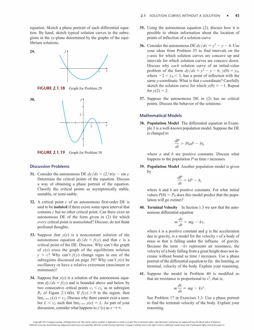
29. f
c y
FIGURE 2.1.18 Graph for Problem 29
30. f
y1
1
FIGURE 2.1.19 Graph for Problem 30
Discussion Problems
31. Consider the autonomous DE dydx (2)y sin y.Determine the critical points of the equation. Discussa way of obtaining a phase portrait of the equation.Classify the critical points as asymptotically stable,unstable, or semi-stable.
32. A critical point c of an autonomous first-order DE issaid to be isolated if there exists some open interval thatcontains c but no other critical point. Can there exist anautonomous DE of the form given in (2) for whichevery critical point is nonisolated? Discuss; do not think profound thoughts.
33. Suppose that y(x) is a nonconstant solution of theautonomous equation dydx f (y) and that c is acritical point of the DE. Discuss: Why can’t the graphof y(x) cross the graph of the equilibrium solutiony c? Why can’t f (y) change signs in one of thesubregions discussed on page 39? Why can’t y(x) beoscillatory or have a relative extremum (maximum orminimum)?
34. Suppose that y(x) is a solution of the autonomous equa-tion dydx f (y) and is bounded above and below bytwo consecutive critical points c1 c2, as in subregion R2 of Figure 2.1.6(b). If f (y) 0 in the region, then limx: y(x) c2. Discuss why there cannot exist a num-ber L c2 such that limx: y(x) L. As part of yourdiscussion, consider what happens to y(x) as x : .
2.1 SOLUTION CURVES WITHOUT A SOLUTION 45
equation. Sketch a phase portrait of each differential equa-tion. By hand, sketch typical solution curves in the subre-gions in the xy-plane determined by the graphs of the equi-librium solutions.
35. Using the autonomous equation (2), discuss how it ispossible to obtain information about the location ofpoints of inflection of a solution curve
36. Consider the autonomous DE dydx y2 y 6. Useyour ideas from Problem 35 to find intervals on they-axis for which solution curves are concave up andintervals for which solution curves are concave down.Discuss why each solution curve of an initial-valueproblem of the form dydx y2 y 6, y(0) y0,where 2 y0 3, has a point of inflection with thesame y-coordinate. What is that y-coordinate? Carefullysketch the solution curve for which y(0) 1. Repeatfor y(2) 2.
37. Suppose the autonomous DE in (2) has no criticalpoints. Discuss the behavior of the solutions.
Mathematical Models
38. Population Model The differential equation in Exam-ple 3 is a well-known population model. Suppose the DEis changed to
,
where a and b are positive constants. Discuss whathappens to the population P as time t increases.
39. Population Model Another population model is given by
,
where h and k are positive constants. For what initialvalues P(0) P0 does this model predict that the popu-lation will go extinct?
40. Terminal Velocity In Section 1.3 we saw that the auto-nomous differential equation
,
where k is a positive constant and g is the accelerationdue to gravity, is a model for the velocity v of a body ofmass m that is falling under the influenc of gravity.Because the term kv represents air resistance, thevelocity of a body falling from a great height does not in-crease without bound as time t increases. Use a phaseportrait of the differential equation to fin the limiting, orterminal, velocity of the body. Explain your reasoning.
41. Suppose the model in Problem 40 is modified so that air resistance is proportional to v2, that is,
.
See Problem 17 in Exercises 1.3. Use a phase portraitto find the terminal velocity of the body. Explain yourreasoning.
m dv
dt mg kv2
m dv
dt mg kv
dP
dt kP h
dP
dt P(aP b)
Copyright 2012 Cengage Learning. All Rights Reserved. May not be copied, scanned, or duplicated, in whole or in part. Due to electronic rights, some third party content may be suppressed from the eBook and/or eChapter(s).
Editorial review has deemed that any suppressed content does not materially affect the overall learning experience. Cengage Learning reserves the right to remove additional content at any time if subsequent rights restrictions require it.
46 CHAPTER 2 FIRST-ORDER DIFFERENTIAL EQUATIONS
42. Chemical Reactions When certain kinds of chemicalsare combined, the rate at which the new compound isformed is modeled by the autonomous differentialequation
where k 0 is a constant of proportionality and 0. Here X(t) denotes the number of grams ofthe new compound formed in time t.
(a) Use a phase portrait of the differential equation topredict the behavior of X(t) as t : .
dX
dt k( X)( X),
(b) Consider the case when . Use a phase portraitof the differential equation to predict the behaviorof X(t) as t : when X(0) . When X(0) .
(c) Verify that an explicit solution of the DE in the casewhen k 1 and is X(t) 1(t c).Find a solution that satisfies X(0) 2. Then fina solution that satisfies X(0) 2. Graph thesetwo solutions. Does the behavior of the solutions ast : agree with your answers to part (b)?
Solution by Integration Consider the first-order differential equation dydx f (x, y). When f does not depend on the variable y, that is, f (x, y) g(x), the differen-tial equation
(1)
can be solved by integration. If g(x) is a continuous function, then integrating bothsides of (1) gives , where G(x) is an antiderivative (indefinite integral) of g(x). For example, if dydx 1 e2x, then its solution is
or .
A Definition Equation (1), as well as its method of solution, is just a specialcase when the function f in the normal form dydx f (x, y) can be factored into afunction of x times a function of y.
y x 12e2x cy (1 e2x) dx
y g(x) dx G(x) c
dy
dx g(x)
DEFINITION 2.2.1 Separable Equation
A first-order di ferential equation of the form
is said to be separable or to have separable variables.
dy
dx g(x)h(y)
For example, the equations
dy
dx y2xe3x4y and
dy
dx y sin x
SEPARABLE EQUATIONS
REVIEW MATERIAL Basic integration formulas (See inside front cover) Techniques of integration: integration by parts and partial fraction decomposition See also the Student Resource Manual.
INTRODUCTION We begin our study of how to solve differential equations with the simplestof all differential equations: first-order equations with separable variables. Because the method inthis section and many techniques for solving differential equations involve integration, you areurged to refresh your memory on important formulas (such as duu) and techniques (such asintegration by parts) by consulting a calculus text.
2.2
Copyright 2012 Cengage Learning. All Rights Reserved. May not be copied, scanned, or duplicated, in whole or in part. Due to electronic rights, some third party content may be suppressed from the eBook and/or eChapter(s).
Editorial review has deemed that any suppressed content does not materially affect the overall learning experience. Cengage Learning reserves the right to remove additional content at any time if subsequent rights restrictions require it.

are separable and nonseparable, respectively. In the first equation we can factorf (x, y) y2xe3x4y as
g(x) h(y)p p
,
but in the second equation there is no way of expressing y sin x as a product of afunction of x times a function of y.
Observe that by dividing by the function h(y), we can write a separable equationdydx g(x)h(y) as
, (2)
where, for convenience, we have denoted 1h(y) by p(y). From this last form we cansee immediately that (2) reduces to (1) when h(y) 1.
Now if y (x) represents a solution of (2), we must have p( (x))(x) g(x),and therefore
. (3)
But dy (x) dx, and so (3) is the same as
, (4)
where H(y) and G(x) are antiderivatives of p(y) 1h(y) and g(x), respectively.
Method of Solution Equation (4) indicates the procedure for solving separableequations. A one-parameter family of solutions, usually given implicitly, is obtainedby integrating both sides of p(y) dy g(x) dx.
Note There is no need to use two constants in the integration of a separableequation, because if we write H(y) c1 G(x) c2, then the difference c2 c1 canbe replaced by a single constant c, as in (4). In many instances throughout the chap-ters that follow, we will relabel constants in a manner convenient to a given equation.For example, multiples of constants or combinations of constants can sometimes bereplaced by a single constant.
p(y) dy g(x) dx or H(y) G(x) c
p( (x))(x) dx g(x) dx
p(y) dy
dx g(x)
f (x, y) y2xe3x4y (xe3x )( y2e4y )
2.2 SEPARABLE EQUATIONS 47
EXAMPLE 1 Solving a Separable DE
Solve (1 x) dy y dx 0.
SOLUTION Dividing by (1 x)y, we can write dyy dx(1 x), from which itfollows that
; laws of exponents
Relabeling as c then gives y c(1 x). ec1
ec1(1 x).
1 x ec1
y eln1xc1 eln1x ec1
ln y ln 1 x c1
dy
y
dx
1 x
; 1 x 1 x,
1 x (1 x),
x 1
x <1
Copyright 2012 Cengage Learning. All Rights Reserved. May not be copied, scanned, or duplicated, in whole or in part. Due to electronic rights, some third party content may be suppressed from the eBook and/or eChapter(s).
Editorial review has deemed that any suppressed content does not materially affect the overall learning experience. Cengage Learning reserves the right to remove additional content at any time if subsequent rights restrictions require it.
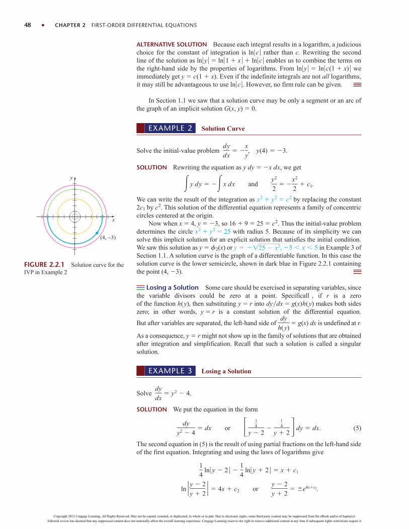
FIGURE 2.2.1 Solution curve for theIVP in Example 2
x
y
(4, −3)
48 CHAPTER 2 FIRST-ORDER DIFFERENTIAL EQUATIONS
ALTERNATIVE SOLUTION Because each integral results in a logarithm, a judiciouschoice for the constant of integration is lnc rather than c. Rewriting the secondline of the solution as lny ln1 x lnc enables us to combine the terms onthe right-hand side by the properties of logarithms. From lny lnc(1 x) weimmediately get y c(1 x). Even if the indefinite integrals are not all logarithms,it may still be advantageous to use lnc . However, no firm rule can be given.
In Section 1.1 we saw that a solution curve may be only a segment or an arc ofthe graph of an implicit solution G(x, y) 0.
EXAMPLE 2 Solution Curve
Solve the initial-value problem .
SOLUTION Rewriting the equation as y dy x dx, we get
.
We can write the result of the integration as x2 y2 c2 by replacing the constant2c1 by c2. This solution of the differential equation represents a family of concentriccircles centered at the origin.
Now when x 4, y 3, so 16 9 25 c2. Thus the initial-value problemdetermines the circle x2 y2 25 with radius 5. Because of its simplicity we cansolve this implicit solution for an explicit solution that satisfies the initial condition.We saw this solution as y 2(x) or in Example 3 ofSection 1.1. A solution curve is the graph of a differentiable function. In this case thesolution curve is the lower semicircle, shown in dark blue in Figure 2.2.1 containingthe point (4, 3).
Losing a Solution Some care should be exercised in separating variables, sincethe variable divisors could be zero at a point. Specificall , if r is a zero of the function h(y), then substituting y r into dydx g(x)h(y) makes both sideszero; in other words, y r is a constant solution of the differential equation.
But after variables are separated, the left-hand side of g(x) dx is undefined at r.
As a consequence, y r might not show up in the family of solutions that are obtainedafter integration and simplification. Recall that such a solution is called a singularsolution.
dy
h(y)
y 125 x2, 5 x 5
y dy x dx andy2
2
x2
2 c1
dy
dx
x
y, y(4) 3
EXAMPLE 3 Losing a Solution
Solve .
SOLUTION We put the equation in the form
. (5)
The second equation in (5) is the result of using partial fractions on the left-hand sideof the first equation. Integrating and using the laws of logarithms give
. ln y 2
y 2 4x c2 ory 2
y 2 e4xc2
1
4 ln y 2
1
4 ln y 2 x c1
dy
y2 4 dx or 1
4
y 2
14
y 2 dy dx
dy
dx y2 4
Copyright 2012 Cengage Learning. All Rights Reserved. May not be copied, scanned, or duplicated, in whole or in part. Due to electronic rights, some third party content may be suppressed from the eBook and/or eChapter(s).
Editorial review has deemed that any suppressed content does not materially affect the overall learning experience. Cengage Learning reserves the right to remove additional content at any time if subsequent rights restrictions require it.

2.2 SEPARABLE EQUATIONS 49
EXAMPLE 4 An Initial-Value Problem
Solve .
SOLUTION Dividing the equation by ey cos x gives
.
Before integrating, we use termwise division on the left-hand side and the trigono-metric identity sin 2x 2 sin x cos x on the right-hand side. Then
integration by parts :
yields ey yey ey 2 cos x c. (7)
The initial condition y 0 when x 0 implies c 4. Thus a solution of the initial-value problem is
ey yey ey 4 2 cos x. (8)
Use of Computers The Remarks at the end of Section 1.1 mentionedthat it may be difficult to use an implicit solution G(x, y) 0 to find an explicitsolution y (x). Equation (8) shows that the task of solving for y in terms of x maypresent more problems than just the drudgery of symbol pushing—sometimes itsimply cannot be done! Implicit solutions such as (8) are somewhat frustrating; nei-ther the graph of the equation nor an interval over which a solution satisfying y(0) 0 is defined is apparent. The problem of “seeing” what an implicit solution looks likecan be overcome in some cases by means of technology. One way* of proceeding isto use the contour plot application of a computer algebra system (CAS). Recall frommultivariate calculus that for a function of two variables z G(x, y) the two-dimensional curves defined by G(x, y) c, where c is constant, are called the levelcurves of the function. With the aid of a CAS, some of the level curves of the func-tion G(x, y) ey yey ey 2 cos x have been reproduced in Figure 2.2.2. Thefamily of solutions defined by (7) is the level curves G(x, y) c. Figure 2.2.3 illus-trates the level curve G(x, y) 4, which is the particular solution (8), in blue color.The other curve in Figure 2.2.3 is the level curve G(x, y) 2, which is the memberof the family G(x, y) c that satisfies y(2) 0.
If an initial condition leads to a particular solution by yielding a specific value ofthe parameter c in a family of solutions for a first-order differential equation, there is
(ey yey) dy 2 sin x dx
e2y y
ey dy sin 2x
cos x dx
(e2y y) cos x dy
dx ey sin 2x, y(0) 0
Here we have replaced 4c1 by c2. Finally, after replacing by c and solving thelast equation for y, we get the one-parameter family of solutions
. (6)
Now if we factor the right-hand side of the differential equation as dydx (y 2)(y 2), we know from the discussion of critical points in Section 2.1that y 2 and y 2 are two constant (equilibrium) solutions. The solution y 2 is amember of the family of solutions defined by (6) corresponding to the value c 0.However, y 2 is a singular solution; it cannot be obtained from (6) for any choice ofthe parameter c. This latter solution was lost early on in the solution process. Inspectionof (5) clearly indicates that we must preclude y 2 in these steps.
y 2 1 ce4x
1 ce4x
ec2
*In Section 2.6 we will discuss several other ways of proceeding that are based on the concept of anumerical solver.
x
y
2_2_2
_1
1
2
_1 1FIGURE 2.2.2 Level curves ofG(x, y) ey yey ey 2 cos x
FIGURE 2.2.3 Level curves c 2 and c 4
(0, 0) /2,0) ( π x
y
2_2_2
_1
1
2
_1 1
c=4
c=2
Copyright 2012 Cengage Learning. All Rights Reserved. May not be copied, scanned, or duplicated, in whole or in part. Due to electronic rights, some third party content may be suppressed from the eBook and/or eChapter(s).
Editorial review has deemed that any suppressed content does not materially affect the overall learning experience. Cengage Learning reserves the right to remove additional content at any time if subsequent rights restrictions require it.
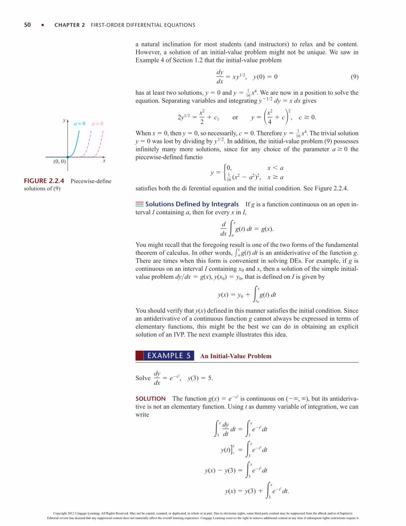
a = >0 a 0
(0, 0) x
y
FIGURE 2.2.4 Piecewise-definesolutions of (9)
50 CHAPTER 2 FIRST-ORDER DIFFERENTIAL EQUATIONS
a natural inclination for most students (and instructors) to relax and be content.However, a solution of an initial-value problem might not be unique. We saw inExample 4 of Section 1.2 that the initial-value problem
(9)
has at least two solutions, y 0 and . We are now in a position to solve theequation. Separating variables and integrating y1/2 dy x dx gives
When x 0, then y 0, so necessarily, c 0. Therefore . The trivial solutiony 0 was lost by dividing by y1/2. In addition, the initial-value problem (9) possessesinfinitely many more solutions, since for any choice of the parameter a 0 thepiecewise-defined functio
satisfies both the di ferential equation and the initial condition. See Figure 2.2.4.
Solutions Defined by Integrals If g is a function continuous on an open in-terval I containing a, then for every x in I,
You might recall that the foregoing result is one of the two forms of the fundamentaltheorem of calculus. In other words, is an antiderivative of the function g.There are times when this form is convenient in solving DEs. For example, if g iscontinuous on an interval I containing x0 and x, then a solution of the simple initial-value problem , that is defined on I is given by
You should verify that y(x) defined in this manner satisfies the initial condition. Sincean antiderivative of a continuous function g cannot always be expressed in terms ofelementary functions, this might be the best we can do in obtaining an explicitsolution of an IVP. The next example illustrates this idea.
y(x) y0 x
x0
g(t) dt
dy>dx g(x), y(x0) y0
xa g(t) dt
d
dx x
ag(t) dt g(x).
y 0,116 (x
2 a2)2,
x a
x a
y 116 x
4
2y1/2 x2
2 c1 or y x2
4 c
2
, c 0.
y 116 x
4
dy
dx xy1/2, y(0) 0
EXAMPLE 5 An Initial-Value Problem
Solve
SOLUTION The function is continuous on , but its antideriva-tive is not an elementary function. Using t as dummy variable of integration, we canwrite
y(x) y(3) x
3et2
dt.
y(x) y(3) x
3et2
dt
y(t)]x
3 x
3et2
dt
x
3 dy
dt dt x
3et2
dt
(, )g(x) ex2
dy
dx ex2
, y(3) 5.
Copyright 2012 Cengage Learning. All Rights Reserved. May not be copied, scanned, or duplicated, in whole or in part. Due to electronic rights, some third party content may be suppressed from the eBook and/or eChapter(s).
Editorial review has deemed that any suppressed content does not materially affect the overall learning experience. Cengage Learning reserves the right to remove additional content at any time if subsequent rights restrictions require it.

Using the initial condition y(3) 5, we obtain the solution
The procedure demonstrated in Example 5 works equally well on separableequations where, say, f (y) possesses an elementary antiderivativebut g(x) does not possess an elementary antiderivative. See Problems 29 and 30 inExercises 2.2.
dy>dx g(x) f (y)
y(x) 5 x
3et2
dt.
2.2 SEPARABLE EQUATIONS 51
REMARKS
(i) As we have just seen in Example 5, some simple functions do not possessan antiderivative that is an elementary function. Integrals of these kinds offunctions are called nonelementary. For example, and arenonelementary integrals. We will run into this concept again in Section 2.3.
(ii) In some of the preceding examples we saw that the constant in the one-parameter family of solutions for a first-order differential equation can be rela-beled when convenient. Also, it can easily happen that two individuals solving thesame equation correctly arrive at dissimilar expressions for their answers. Forexample, by separation of variables we can show that one-parameter families ofsolutions for the DE (1 y2) dx (1 x2) dy 0 are
.
As you work your way through the next several sections, bear in mind that fami-lies of solutions may be equivalent in the sense that one family may be obtainedfrom another by either relabeling the constant or applying algebra and trigonom-etry. See Problems 27 and 28 in Exercises 2.2.
arctan x arctan y c orx y
1 xy c
sin x2 dxx3 et2
dt
EXERCISES 2.2 Answers to selected odd-numbered problems begin on page ANS-2.
In Problems 1–22 solve the given differential equation byseparation of variables.
1. 2.
3. dx e3xdy 0 4. dy (y 1)2dx 0
5. 6.
7. 8.
9. 10.
11. csc y dx sec2x dy 0
12. sin 3x dx 2y cos33x dy 0
13. (ey 1)2ey dx (ex 1)3ex dy 0
14. x(1 y2)1/2 dx y(1 x2)1/2 dy
dy
dx 2y 3
4x 52
y ln x dx
dy y 1
x 2
exy dy
dx ey e2xydy
dx e3x2y
dy
dx 2xy2 0x
dy
dx 4y
dy
dx (x 1)2dy
dx sin 5x
15. 16.
17. 18.
19. 20.
21. 22.
In Problems 23–28 find an explicit solution of the giveninitial-value problem.
23.
24.
25. x2 dy
dx y xy, y(1) 1
dy
dx
y2 1
x2 1, y(2) 2
dx
dt 4(x2 1), x(>4) 1
(ex ex) dy
dx y2dy
dx x11 y2
dy
dx
xy 2y x 2
xy 3y x 3
dy
dx
xy 3x y 3
xy 2x 4y 8
dN
dt N Ntet2dP
dt P P2
dQ
dt k(Q 70)
dS
dr kS
Copyright 2012 Cengage Learning. All Rights Reserved. May not be copied, scanned, or duplicated, in whole or in part. Due to electronic rights, some third party content may be suppressed from the eBook and/or eChapter(s).
Editorial review has deemed that any suppressed content does not materially affect the overall learning experience. Cengage Learning reserves the right to remove additional content at any time if subsequent rights restrictions require it.

52 CHAPTER 2 FIRST-ORDER DIFFERENTIAL EQUATIONS
26.
27.
28. (1 x4) dy x(1 4y2) dx 0, y(1) 0
In Problems 29 and 30 proceed as in Example 5 and find anexplicit solution of the given initial-value problem.
29.
30.
In Problems 31–34 find an explicit solution of the giveninitial-value problem. Determine the exact interval I of definition by analytical methods. Use a graphing utility to plotthe graph of the solution.
31.
32.
33.
34.
35. (a) Find a solution of the initial-value problem consist-ing of the differential equation in Example 3 andeach of the initial-conditions: y(0) 2, y(0) 2,and .
(b) Find the solution of the differential equation inExample 4 when ln c1 is used as the constant ofintegration on the left-hand side in the solution and4 ln c1 is replaced by ln c. Then solve the sameinitial-value problems in part (a).
36. Find a solution of that passes through
the indicated points.
(a) (0, 1) (b) (0, 0) (c) (d)
37. Find a singular solution of Problem 21. Of Problem 22.
38. Show that an implicit solution of
is given by ln(x2 10) csc y c. Find the constantsolutions, if any, that were lost in the solution of the dif-ferential equation.
Often a radical change in the form of the solution of a differen-tial equation corresponds to a very small change in either theinitial condition or the equation itself. In Problems 39–42 finan explicit solution of the given initial-value problem. Use agraphing utility to plot the graph of each solution. Compareeach solution curve in a neighborhood of (0, 1).
39.dy
dx (y 1)2, y(0) 1
2x sin2 y dx (x2 10) cos y dy 0
(2, 14)(12,
12)
xdy
dx y2 y
y (14) 1
sin x dx ydy 0, y(0) 1
eydx exdy 0, y(0) 0
(2y 2) dy
dx 3x2 4x 2, y(1) 2
dy
dx
2x 1
2y, y(2) 1
dy
dx y 2 sin x2, y(2) 1
3
dy
dx yex2
, y(4) 1
11 y2 dx 11 x2 dy 0, y(0) 13
2
dy
dt 2y 1, y(0) 5
240.
41.
42.
43. Every autonomous first-orde equation dydx f (y)is separable. Find explicit solutions y1(x), y2(x), y3(x),and y4(x) of the differential equation dydx y y3
that satisfy, in turn, the initial conditions y1(0) 2,, , and y4(0) 2. Use a graphing
utility to plot the graphs of each solution. Compare thesegraphs with those predicted in Problem 19 of Exercises 2.1.Give the exact interval of definitio for each solution.
44. (a) The autonomous first-order differential equation dydx 1(y 3) has no critical points.Nevertheless, place 3 on the phase line and obtaina phase portrait of the equation. Compute d2ydx2
to determine where solution curves are concave upand where they are concave down (see Problems35 and 36 in Exercises 2.1). Use the phase portraitand concavity to sketch, by hand, some typicalsolution curves.
(b) Find explicit solutions y1(x), y2(x), y3(x), and y4(x)of the differential equation in part (a) that satisfy,in turn, the initial conditions y1(0) 4, y2(0) 2,y3(1) 2, and y4(1) 4. Graph each solutionand compare with your sketches in part (a). Givethe exact interval of definition for each solution.
In Problems 45–50 use a technique of integration or a substi-tution to find an explicit solution of the given differentialequation or initial-value problem.
45. 46.
47. 48.
49. 50.
Discussion Problems
51. (a) Explain why the interval of definition of the explicitsolution y 2(x) of the initial-value problem inExample 2 is the open interval (5, 5).
(b) Can any solution of the differential equation crossthe x-axis? Do you think that x2 y2 1 is animplicit solution of the initial-value problem dydx xy, y(1) 0?
52. (a) If a 0, discuss the differences, if any, betweenthe solutions of the initial-value problems consist-ing of the differential equation dydx xy and
dy
dx
x tan1 x
y, y(0) 3
dy
dx
e1x
y, y(1) 4
dy
dx y2/3 y(1x x)
dy
dx 1y y
dy
dx
sin1x1y
dy
dx
1
1 sin x
y3(0) 12y2(0) 1
2
dy
dx (y 1)2 0.01, y(0) 1
dy
dx (y 1)2 0.01, y(0) 1
dy
dx (y 1)2, y(0) 1.01
Copyright 2012 Cengage Learning. All Rights Reserved. May not be copied, scanned, or duplicated, in whole or in part. Due to electronic rights, some third party content may be suppressed from the eBook and/or eChapter(s).
Editorial review has deemed that any suppressed content does not materially affect the overall learning experience. Cengage Learning reserves the right to remove additional content at any time if subsequent rights restrictions require it.

each of the initial conditions y(a) a, y(a) a,y(a) a, and y(a) a.
(b) Does the initial-value problem dydx xy,y(0) 0 have a solution?
(c) Solve dydx xy, y(1) 2 and give the exactinterval I of definition of its solution
53. In Problems 43 and 44 we saw that every autonomousfirst-order differential equation dydx f (y) isseparable. Does this fact help in the solution of the
initial-value problem ?
Discuss. Sketch, by hand, a plausible solution curve ofthe problem.
54. (a) Solve the two initial-value problems:
and
(b) Show that there are more than 1.65 million digits inthe y-coordinate of the point of intersection of thetwo solution curves in part (a).
55. Find a function whose square plus the square of itsderivative is 1.
56. (a) The differential equation in Problem 27 is equiva-lent to the normal form
in the square region in the xy-plane defined byx 1, y 1. But the quantity under the radical isnonnegative also in the regions defined by x 1,y 1. Sketch all regions in the xy-plane forwhich this differential equation possesses realsolutions.
(b) Solve the DE in part (a) in the regions defined byx 1, y 1. Then find an implicit and anexplicit solution of the differential equation subjectto y(2) 2.
Mathematical Model
57. Suspension Bridge In (16) of Section 1.3 we saw thata mathematical model for the shape of a flexible cablestrung between two vertical supports is
, (10)
where W denotes the portion of the total vertical loadbetween the points P1 and P2 shown in Figure 1.3.7. The
dy
dx
W
T1
dy
dx B1 y2
1 x2
dy
dx y
y
x ln x, y(e) 1.
dy
dx y, y(0) 1
dy
dx 11 y2 sin2 y, y(0) 1
2
DE (10) is separable under the following conditions thatdescribe a suspension bridge.
Let us assume that the x- and y-axes are as shown inFigure 2.2.5—that is, the x-axis runs along the horizon-tal roadbed, and the y-axis passes through (0, a), whichis the lowest point on one cable over the span of thebridge, coinciding with the interval [L2, L2]. In thecase of a suspension bridge, the usual assumption is thatthe vertical load in (10) is only a uniform roadbed dis-tributed along the horizontal axis. In other words, it isassumed that the weight of all cables is negligible incomparison to the weight of the roadbed and that theweight per unit length of the roadbed (say, pounds perhorizontal foot) is a constant . Use this information toset up and solve an appropriate initial-value problemfrom which the shape (a curve with equation y (x))of each of the two cables in a suspension bridge isdetermined. Express your solution of the IVP in termsof the sag h and span L. See Figure 2.2.5.
2.2 SEPARABLE EQUATIONS 53
FIGURE 2.2.5 Shape of a cable in Problem 57
L/2L (span)
h (sag)
cable
roadbed (load)
x
(0, a)
L/2
y
Computer Lab Assignments
58. (a) Use a CAS and the concept of level curves toplot representative graphs of members of thefamily of solutions of the differential equation
. Experiment with different numbers
of level curves as well as various rectangularregions defined by a x b, c y d.
(b) On separate coordinate axes plot the graphs of theparticular solutions corresponding to the initialconditions: y(0) 1; y(0) 2; y(1) 4;y(1) 3.
59. (a) Find an implicit solution of the IVP
(b) Use part (a) to find an explicit solution y (x) ofthe IVP.
(c) Consider your answer to part (b) as a function only.Use a graphing utility or a CAS to graph this func-tion, and then use the graph to estimate its domain.
(d) With the aid of a root-finding application of a CAS,determine the approximate largest interval I of
(2y 2) dy (4x3 6x) dx 0, y(0) 3.
dy
dx
8x 5
3y2 1
Copyright 2012 Cengage Learning. All Rights Reserved. May not be copied, scanned, or duplicated, in whole or in part. Due to electronic rights, some third party content may be suppressed from the eBook and/or eChapter(s).
Editorial review has deemed that any suppressed content does not materially affect the overall learning experience. Cengage Learning reserves the right to remove additional content at any time if subsequent rights restrictions require it.
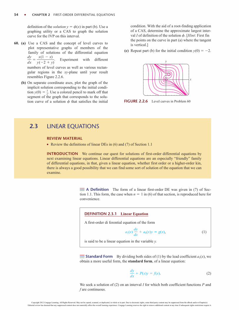
54 CHAPTER 2 FIRST-ORDER DIFFERENTIAL EQUATIONS
definition of the solution y (x) in part (b). Use agraphing utility or a CAS to graph the solutioncurve for the IVP on this interval.
60. (a) Use a CAS and the concept of level curves toplot representative graphs of members of thefamily of solutions of the differential equation
. Experiment with different
numbers of level curves as well as various rectan-gular regions in the xy-plane until your resultresembles Figure 2.2.6.
(b) On separate coordinate axes, plot the graph of theimplicit solution corresponding to the initial condi-tion . Use a colored pencil to mark off thatsegment of the graph that corresponds to the solu-tion curve of a solution that satisfies the initial
y(0) 32
dy
dx
x(1 x)
y(2 y)
condition. With the aid of a root-finding applicationof a CAS, determine the approximate largest inter-val I of definition of the solution . [Hint: First finthe points on the curve in part (a) where the tangentis vertical.]
(c) Repeat part (b) for the initial condition y(0) 2.
x
y
FIGURE 2.2.6 Level curves in Problem 60
LINEAR EQUATIONS
REVIEW MATERIAL Review the definitions of linear DEs in (6) and (7) of Section 1.1
INTRODUCTION We continue our quest for solutions of first-order differential equations bynext examining linear equations. Linear differential equations are an especially “friendly” familyof differential equations, in that, given a linear equation, whether first order or a higher-order kin,there is always a good possibility that we can find some sort of solution of the equation that we canexamine.
2.3
A Definition The form of a linear first-order DE was given in (7) of Sec-tion 1.1. This form, the case when in (6) of that section, is reproduced here forconvenience.
n 1
DEFINITION 2.3.1 Linear Equation
A first-order di ferential equation of the form
, (1)
is said to be a linear equation in the variable y.
a1(x) dy
dx a0(x)y g(x)
Standard Form By dividing both sides of (1) by the lead coefficient weobtain a more useful form, the standard form, of a linear equation:
(2)
We seek a solution of (2) on an interval I for which both coefficient functions P andf are continuous.
dy
dx P(x)y f (x).
a1(x),
Copyright 2012 Cengage Learning. All Rights Reserved. May not be copied, scanned, or duplicated, in whole or in part. Due to electronic rights, some third party content may be suppressed from the eBook and/or eChapter(s).
Editorial review has deemed that any suppressed content does not materially affect the overall learning experience. Cengage Learning reserves the right to remove additional content at any time if subsequent rights restrictions require it.

2.3 LINEAR EQUATIONS 55
Before we examine a general procedure for solving equations of form (2) wenote that in some instances (2) can be solved by separation of variables. For exam-ple, you should verify that the equations
and
are both linear and separable, but that the linear equation
is not separable.
Method of Solution The method for solving (2) hinges on a remarkable factthat the left-hand side of the equation can be recast into the form of the exact deriva-tive of a product by multiplying the both sides of (2) by a special function It isrelatively easy to find the function because we want
left hand side of product product rule (2) multipled by m(x) 2 4 4
c cthese must be equal
The equality is true provided that
The last equation can be solved by separation of variables. Integrating
gives . Even though there are an infinite choices of (all constantmultiples of ), all produce the same desired result. Hence we can simplify lifeand choose The function
(3)
is called an integrating factor for equation (2). Here is what we have so far: We multiplied both sides of (2) by (3) and, by
construction, the left-hand side is the derivative of a product of the integrating factorand y:
Finally, we discover why (3) is called an integrating factor. We can integrate bothsides of the last equation,
and solve for y. The result is a one-parameter family of solutions of (2):
(4)
We emphasize that you should not memorize formula (4). The following proce-dure should be worked through each time.
y eP(x)dx eP(x)dx f(x)dx ceP(x)dx.
eP(x)dx y eP(x)dx f(x) c
d
dx [eP(x)dx y] eP(x)dx f(x).
eP(x)dx dy
dx P(x)eP(x)dx y eP(x)dx f(x)
(x) eP(x)dx
c2 1.eP(x)dx
(x)(x) c2eP(x)dx
d
Pdx and solving ln(x) P(x)dx c1
d
dx P.
d
dx [(x)y]
dy
dx
d
dxy
dy
dx Py.
(x)(x).
dy
dx y x
dy
dx y 5
dy
dx 2xy 0
We match each equation with (2). In thefirst equation P(x) 2x, f(x) 0 and inthe second P(x) 1, f(x) 5.
See Problem 50 in Exercises 2.3
Copyright 2012 Cengage Learning. All Rights Reserved. May not be copied, scanned, or duplicated, in whole or in part. Due to electronic rights, some third party content may be suppressed from the eBook and/or eChapter(s).
Editorial review has deemed that any suppressed content does not materially affect the overall learning experience. Cengage Learning reserves the right to remove additional content at any time if subsequent rights restrictions require it.

56 CHAPTER 2 FIRST-ORDER DIFFERENTIAL EQUATIONS
SOLVING A LINEAR FIRST-ORDER EQUATION
(i) Remember to put a linear equation into the standard form (2).
(ii) From the standard form of the equation identify P(x) and then find thintegrating factor eP(x)dx. No constant need be used in evaluating theindefinite integral P(x)dx.
(iii) Multiply the both sides of the standard form equation by the integratingfactor. The left-hand side of the resulting equation is automatically thederivative of the product of the integrating factor eP(x)dx and y:
(iv) Integrate both sides of the last equation and solve for y.
d
dx [eP(x)dxy] eP(x)dx f (x).
EXAMPLE 1 Solving a Linear Equation
Solve
SOLUTION This linear equation can be solved by separation of variables.Alternatively, since the differential equation is already in standard form (2), we iden-tify and so the integrating factor is . We then multiply thegiven equation by this factor and recognize that
Integration of the last equation,
then yields or y ce3x, x .e3xy c
d
dx [e3x y] dx 0 dx
e3x dy
dx 3e3x y e3x 0 is the same as
d
dx [e3x y] 0.
e(3)dx e3xP(x) 3,
dy
dx 3y 0.
EXAMPLE 2 Solving a Linear Equation
Solve
SOLUTION This linear equation, like the one in Example 1, is already in standardform with Thus the integrating factor is again . This time multiply-ing the given equation by this factor gives
Integrating the last equation,
or
When a1, a0, and g in (1) are constants, the differential equation is autonomous.In Example 2 you can verify from the normal form dydx 3(y 2) that 2 is acritical point and that it is unstable (a repeller). Thus a solution curve with an
y 2 ce3x, x .
d
dx [e3x y] dx 6e3x dx gives e3x y 6e3x
3 c,
e3x dy
dx 3e3x y 6e3x and so
d
dx [e3x y] 6e3x.
e3xP(x) 3.
dy
dx 3y 6.
Copyright 2012 Cengage Learning. All Rights Reserved. May not be copied, scanned, or duplicated, in whole or in part. Due to electronic rights, some third party content may be suppressed from the eBook and/or eChapter(s).
Editorial review has deemed that any suppressed content does not materially affect the overall learning experience. Cengage Learning reserves the right to remove additional content at any time if subsequent rights restrictions require it.
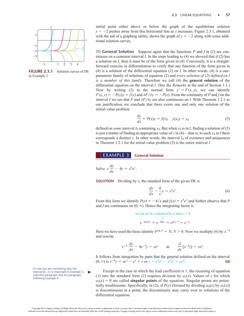
initial point either above or below the graph of the equilibrium solution y 2 pushes away from this horizontal line as x increases. Figure 2.3.1, obtainedwith the aid of a graphing utility, shows the graph of y 2 along with some addi-tional solution curves.
General Solution Suppose again that the functions P and f in (2) are con-tinuous on a common interval I. In the steps leading to (4) we showed that if (2) hasa solution on I, then it must be of the form given in (4). Conversely, it is a straight-forward exercise in differentiation to verify that any function of the form given in(4) is a solution of the differential equation (2) on I. In other words, (4) is a one-parameter family of solutions of equation (2) and every solution of (2) defined on Iis a member of this family. Therefore we call (4) the general solution of thedifferential equation on the interval I. (See the Remarks at the end of Section 1.1.)Now by writing (2) in the normal form y F (x, y), we can identify F (x, y) P(x)y f (x) and Fy P(x). From the continuity of P and f on theinterval I we see that F and Fy are also continuous on I. With Theorem 1.2.1 asour justification, we conclude that there exists one and only one solution of theinitial-value problem
(5)
defined on some interval I0 containing x0. But when x0 is in I, finding a solution of (5)is just a matter of finding an appropriate value of c in (4)—that is, to each x0 in I therecorresponds a distinct c. In other words, the interval I0 of existence and uniquenessin Theorem 1.2.1 for the initial-value problem (5) is the entire interval I.
dy
dx P(x)y f (x), y(x0) y0
2.3 LINEAR EQUATIONS 57
FIGURE 2.3.1 Solution curves of DEin Example 2
1_1 2 3 4
_2_1
1
_3
x
y
y =_2
EXAMPLE 3 General Solution
Solve .
SOLUTION Dividing by x, the standard form of the given DE is
. (6)
From this form we identify P(x) 4x and f (x) x5ex and further observe that Pand f are continuous on (0, ). Hence the integrating factor is
Here we have used the basic identity . Now we multiply (6) by x4
and rewrite
It follows from integration by parts that the general solution defined on the interval(0, ) is x4y xex ex c or y x5ex x4ex cx4.
Except in the case in which the lead coefficient is 1, the recasting of equation(1) into the standard form (2) requires division by a1(x). Values of x for whicha1(x) 0 are called singular points of the equation. Singular points are poten-tially troublesome. Specifically, in (2), if P(x) (formed by dividing a0(x) by a1(x))is discontinuous at a point, the discontinuity may carry over to solutions of thedifferential equation.
x4 dy
dx 4x5y xex as
d
dx [x4y] xex.
blogbN N, N 0
e4dx/x e4ln x eln x4 x4.
we can use ln x instead of ln x since x 0
dy
dx
4
x y x5ex
x dy
dx 4y x6ex
In case you are wondering why theinterval (0, ) is important in Example 3,read this paragraph and the paragraphfollowing Example 4.
Copyright 2012 Cengage Learning. All Rights Reserved. May not be copied, scanned, or duplicated, in whole or in part. Due to electronic rights, some third party content may be suppressed from the eBook and/or eChapter(s).
Editorial review has deemed that any suppressed content does not materially affect the overall learning experience. Cengage Learning reserves the right to remove additional content at any time if subsequent rights restrictions require it.

58 CHAPTER 2 FIRST-ORDER DIFFERENTIAL EQUATIONS
EXAMPLE 4 General Solution
Find the general solution of .
SOLUTION We write the differential equation in standard form
(7)
and identify P(x) x(x2 9). Although P is continuous on (, 3), (3, 3), and(3, ), we shall solve the equation on the first and third intervals. On these intervalsthe integrating factor is
.
After multiplying the standard form (7) by this factor, we get
.
Integrating both sides of the last equation gives Thus for either
x 3 or x 3 the general solution of the equation is .
Notice in Example 4 that x 3 and x 3 are singular points of the equationand that every function in the general solution is discontinuous atthese points. On the other hand, x 0 is a singular point of the differential equationin Example 3, but the general solution y x5ex x4ex cx4 is noteworthy in thatevery function in this one-parameter family is continuous at x 0 and is defineon the interval (, ) and not just on (0, ), as stated in the solution. However,the family y x5ex x4ex cx4 defined on (, ) cannot be considered the gen-eral solution of the DE, since the singular point x 0 still causes a problem. SeeProblems 45 and 46 in Exercises 2.3.
y c1x2 9
y c1x2 9
1x2 9 y c.
d
dx 1x2 9 y 0
ex dx/(x29) e12 2x dx/(x29) e
12 lnx29 1x2 9
dy
dx
x
x2 9 y 0
(x2 9) dy
dx xy 0
EXAMPLE 5 An Initial-Value Problem
Solve .
SOLUTION The equation is in standard form, and P(x) 1 and f (x) x are contin-uous on (, ). The integrating factor is edx ex, so integrating
gives exy xex ex c. Solving this last equation for y yields the general solutiony x 1 cex. But from the initial condition we know that y 4 when x 0.Substituting these values into the general solution implies that c 5. Hence thesolution of the problem is
y x 1 5ex, x . (8)
Figure 2.3.2, obtained with the aid of a graphing utility, shows the graph ofthe solution (8) in dark blue along with the graphs of other members of the one-parameter family of solutions y x 1 cex. It is interesting to observe that as xincreases, the graphs of all members of this family are close to the graph of the solu-tion The last solution corresponds to in the family and is shown inc 0y x 1.
d
dx [exy] xex
dy
dx y x, y(0) 4
x
y
4_4_4
_2
2
4
_2 2
c=0
c>0 c=5
c<0
FIGURE 2.3.2 Solution curves of DEin Example 5
Copyright 2012 Cengage Learning. All Rights Reserved. May not be copied, scanned, or duplicated, in whole or in part. Due to electronic rights, some third party content may be suppressed from the eBook and/or eChapter(s).
Editorial review has deemed that any suppressed content does not materially affect the overall learning experience. Cengage Learning reserves the right to remove additional content at any time if subsequent rights restrictions require it.

dark green in Figure 2.3.2. This asymptotic behavior of solutions is due to the factthat the contribution of cex, , becomes negligible for increasing values of x.We say that cex is a transient term, since ex : 0 as x : . While this behavioris not characteristic of all general solutions of linear equations (see Example 2), thenotion of a transient is often important in applied problems.
Discontinuous Coefficients In applications, the coefficients P(x) and f (x) in(2) may be piecewise continuous. In the next example f (x) is piecewise continuouson [0, ) with a single discontinuity, namely, a (finite) jump discontinuity at x 1.We solve the problem in two parts corresponding to the two intervals over which f isdefined. It is then possible to piece together the two solutions at x 1 so that y(x) iscontinuous on [0, ).
c 0
2.3 LINEAR EQUATIONS 59
EXAMPLE 6 An Initial-Value Problem
Solve
SOLUTION The graph of the discontinuous function f is shown in Figure 2.3.3. Wesolve the DE for y(x) first on the interval [0, 1] and then on the interval (1, ). For0 x 1 we have
.
Integrating this last equation and solving for y gives y 1 c1ex. Since y(0) 0,we must have c1 1, and therefore y 1 ex, 0 x 1. Then for x 1 theequation
leads to y c2ex. Hence we can write
By appealing to the definition of continuity at a point, it is possible to determine c2 so that the foregoing function is continuous at x 1. The requirement that
implies that c2e1 1 e1 or c2 e 1. As seen inFigure 2.3.4, the function
(9)
is continuous on (0, ).
It is worthwhile to think about (9) and Figure 2.3.4 a little bit; you are urged toread and answer Problem 48 in Exercises 2.3.
Functions Defined by Integrals At the end of Section 2.2 we discussedthe fact that some simple continuous functions do not possess antiderivatives thatare elementary functions and that integrals of these kinds of functions are callednonelementary. For example, you may have seen in calculus that andsin x2 dx are nonelementary integrals. In applied mathematics some important func-tions are define in terms of nonelementary integrals. Two such special functions arethe error function and complementary error function:
. (10)erf(x) 21
x
0 et2
dt and erfc(x) 21
x et2
dt
ex2 dx
y 1 ex,
(e 1)ex,
0 x 1,
x 1
limx:1 y(x) y(1)
y 1 ex,
c2ex,
0 x 1,
x 1.
dy
dx y 0
dy
dx y 1 or, equivalently,
d
dx [exy] ex
dy
dx y f (x), y(0) 0 where f (x) 1,
0,
0 x 1,
x 1.
FIGURE 2.3.3 Discontinuous f(x) inExample 6
x
y
1 x
y
FIGURE 2.3.4 Graph of (9) inExample 6
Copyright 2012 Cengage Learning. All Rights Reserved. May not be copied, scanned, or duplicated, in whole or in part. Due to electronic rights, some third party content may be suppressed from the eBook and/or eChapter(s).
Editorial review has deemed that any suppressed content does not materially affect the overall learning experience. Cengage Learning reserves the right to remove additional content at any time if subsequent rights restrictions require it.

*This result is usually proved in the third semester of calculus.†Certain commands have the same spelling, but in Mathematica commands begin with a capital letter(DSolve), whereas in Maple the same command begins with a lower case letter (dsolve). Whendiscussing such common syntax, we compromise and write, for example, dsolve. See the StudentResource Manual for the complete input commands used to solve a linear first-order DE
FIGURE 2.3.5 Solution curves of DEin Example 7
x
y
60 CHAPTER 2 FIRST-ORDER DIFFERENTIAL EQUATIONS
From the known result * we can write Then from it is seen from (10) that the complementary error func-tion erfc(x) is related to erf(x) by erf(x) erfc(x) 1. Because of its importancein probability, statistics, and applied partial differential equations, the error func-tion has been extensively tabulated. Note that erf(0) 0 is one obvious functionvalue. Values of erf(x) can also be found by using a CAS.
0 x
0 x
(21) 0 et2
dt 1.0 et2
dt 12
EXAMPLE 7 The Error Function
Solve the initial-value problem .
SOLUTION Since the equation is already in standard form, we see that the integrat-ing factor is , so from
. (11)
Applying y(0) 1 to the last expression then gives c 1. Hence the solution of theproblem is
The graph of this solution on the interval (, ), shown in dark blue in Figure 2.3.5among other members of the family defined in (11), was obtained with the aid of acomputer algebra system.
Use of Computers The computer algebra systems Mathematica and Mapleare capable of producing implicit or explicit solutions for some kinds of differentialequations using their dsolve commands.†
y 2ex2 x
0 et2
dt ex2or y ex2
[1 1 erf(x)].
d
dx [ex2
y] 2ex2we get y 2ex2 x
0 et2
dt cex2
ex2
dy
dx 2xy 2, y(0) 1
REMARKS
(i) A linear first-order di ferential equation
is said to be homogeneous, whereas the equation
with not identically zero is said to be nonhomogeneous. For example, thelinear equations and are, in turn, homogeneous andnonhomogeneous. As can be seen in this example the trivial solution isalways a solution of a homogeneous linear DE. Store this terminology in theback of your mind because it becomes important when we study linear higher-order ordinary differential equations in Chapter 4.
y 0xy y exxy y 0
g(x)
a1(x) dy
dx a0(x)y g(x)
a1(x) dy
dx a0(x)y 0
Copyright 2012 Cengage Learning. All Rights Reserved. May not be copied, scanned, or duplicated, in whole or in part. Due to electronic rights, some third party content may be suppressed from the eBook and/or eChapter(s).
Editorial review has deemed that any suppressed content does not materially affect the overall learning experience. Cengage Learning reserves the right to remove additional content at any time if subsequent rights restrictions require it.

2.3 LINEAR EQUATIONS 61
(ii) Occasionally, a first-order differential equation is not linear in one variablebut in linear in the other variable. For example, the differential equation
is not linear in the variable y. But its reciprocal
is recognized as linear in the variable x. You should verify that the integratingfactor and integration by parts yield the explicit solution
for the second equation. This expression is then animplicit solution of the first equation
(iii) Mathematicians have adopted as their own certain words from engineer-ing, which they found appropriately descriptive. The word transient, used ear-lier, is one of these terms. In future discussions the words input and output willoccasionally pop up. The function f in (2) is called the input or driving func-tion; a solution of the differential equation for a given input is called theoutput or response.
(iv) The term special functions mentioned in conjunction with the error func-tion also applies to the sine integral function and the Fresnel sine integralintroduced in Problems 55 and 56 in Exercises 2.3. “Special Functions” isactually a well-defined branch of mathematics. More special functions arestudied in Section 6.4.
y(x)
x y2 2y 2 ceye(1)dy ey
dx
dy x y2 or
dx
dy x y2
dy
dx
1
x y2
EXERCISES 2.3 Answers to selected odd-numbered problems begin on page ANS-2.
In Problems 1–24 find the general solution of the given dif-ferential equation. Give the largest interval I over which thegeneral solution is defined. Determine whether there are anytransient terms in the general solution.
1. 2.
3. 4.
5. y 3x2y x2 6. y 2xy x3
7. x2y xy 1 8. y 2y x2 5
9. 10.
11. 12.
13. x2y x(x 2)y ex
14. xy (1 x)y ex sin 2x
15. y dx 4(x y6) dy 0
16. y dx (yey 2x) dy
17. cos x dy
dx (sin x)y 1
(1 x) dy
dx xy x x2x
dy
dx 4y x3 x
x dy
dx 2y 3x
dy
dx y x2 sin x
3 dy
dx 12y 4
dy
dx y e3x
dy
dx 2y 0
dy
dx 5y
18.
19.
20.
21.
22.
23.
24.
In Problems 25–36 solve the given initial-value problem.Give the largest interval I over which the solution is defined
25.
26.
27. xy y ex, y(1) 2
dy
dx 2x 3y, y(0) 1
3
dy
dx x 5y, y(0) 3
(x2 1) dy
dx 2y (x 1)2
x dy
dx (3x 1)y e3x
dP
dt 2tP P 4t 2
dr
d r sec cos
(x 2)2 dy
dx 5 8y 4xy
(x 1) dy
dx (x 2)y 2xex
cos2x sin x dy
dx (cos3x)y 1
Copyright 2012 Cengage Learning. All Rights Reserved. May not be copied, scanned, or duplicated, in whole or in part. Due to electronic rights, some third party content may be suppressed from the eBook and/or eChapter(s).
Editorial review has deemed that any suppressed content does not materially affect the overall learning experience. Cengage Learning reserves the right to remove additional content at any time if subsequent rights restrictions require it.
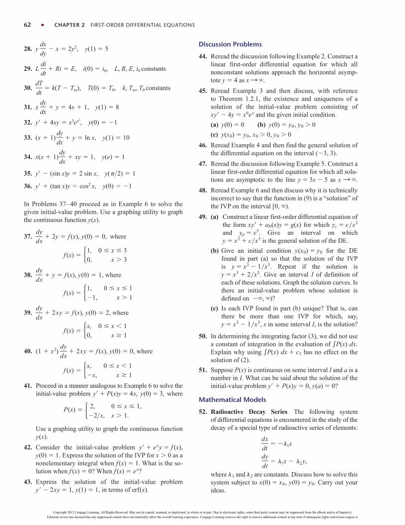
62 CHAPTER 2 FIRST-ORDER DIFFERENTIAL EQUATIONS
28.
29.
30.
31.
32.
33.
34.
35.
36.
In Problems 37–40 proceed as in Example 6 to solve thegiven initial-value problem. Use a graphing utility to graphthe continuous function y(x).
37. where
38. where
39. where
40. where
41. Proceed in a manner analogous to Example 6 to solve theinitial-value problem y P(x)y 4x, y(0) 3, where
Use a graphing utility to graph the continuous functiony(x).
42. Consider the initial-value problem y exy f (x),y(0) 1. Express the solution of the IVP for x 0 as anonelementary integral when f (x) 1. What is the so-lution when f (x) 0? When f (x) ex?
43. Express the solution of the initial-value problem y 2xy 1, y(1) 1, in terms of erf(x).
P(x) 2,
2>x,
0 x 1,
x 1.
f (x) x,
x,
0 x 1
x 1
(1 x2) dy
dx 2xy f (x), y(0) 0,
f (x) x,
0,
0 x 1
x 1
dy
dx 2xy f (x), y(0) 2,
f (x) 1,
1,
0 x 1
x 1
dy
dx y f (x), y(0) 1,
f (x) 1,
0,
0 x 3
x 3
dy
dx 2y f (x), y(0) 0,
y (tan x)y cos2 x, y(0) 1
y (sin x)y 2 sin x, y(>2) 1
x(x 1)dy
dx xy 1, y(e) 1
(x 1)dy
dx y ln x, y(1) 10
y 4xy x3ex2, y(0) 1
xdy
dx y 4x 1, y(1) 8
dT
dt k(T Tm), T(0) T0, k, Tm, T0 constants
Ldi
dt Ri E, i(0) i0, L, R, E, i0 constants
ydx
dy x 2y2, y(1) 5
Discussion Problems
44. Reread the discussion following Example 2. Construct alinear first-order differential equation for which allnonconstant solutions approach the horizontal asymp-tote y 4 as x : .
45. Reread Example 3 and then discuss, with referenceto Theorem 1.2.1, the existence and uniqueness of asolution of the initial-value problem consisting of xy 4y x6ex and the given initial condition.
(a) y(0) 0 (b) y(0) y0, y0 0
(c) y(x0) y0, x0 0, y0 0
46. Reread Example 4 and then find the general solution ofthe differential equation on the interval (3, 3).
47. Reread the discussion following Example 5. Construct alinear first-order differential equation for which all solu-tions are asymptotic to the line y 3x 5 as x : .
48. Reread Example 6 and then discuss why it is technicallyincorrect to say that the function in (9) is a “solution” ofthe IVP on the interval [0, ).
49. (a) Construct a linear first-order differential equation ofthe form xy a0(x)y g(x) for which yc cx3
and yp x3. Give an interval on which y x3 cx3 is the general solution of the DE.
(b) Give an initial condition y(x0) y0 for the DEfound in part (a) so that the solution of the IVPis y x3 1x3. Repeat if the solution is y x3 2x3. Give an interval I of definition ofeach of these solutions. Graph the solution curves. Isthere an initial-value problem whose solution isdefined on , )?
(c) Is each IVP found in part (b) unique? That is, canthere be more than one IVP for which, say, y x3 1x3, x in some interval I, is the solution?
50. In determining the integrating factor (3), we did not usea constant of integration in the evaluation of P(x) dx.Explain why using P(x) dx c1 has no effect on thesolution of (2).
51. Suppose P(x) is continuous on some interval I and a is anumber in I. What can be said about the solution of theinitial-value problem y P(x)y 0, y(a) 0?
Mathematical Models
52. Radioactive Decay Series The following systemof differential equations is encountered in the study of thedecay of a special type of radioactive series of elements:
where 1 and 2 are constants. Discuss how to solve thissystem subject to x(0) x0, y(0) y0. Carry out yourideas.
dy
dt 1x 2y,
dx
dt 1x
Copyright 2012 Cengage Learning. All Rights Reserved. May not be copied, scanned, or duplicated, in whole or in part. Due to electronic rights, some third party content may be suppressed from the eBook and/or eChapter(s).
Editorial review has deemed that any suppressed content does not materially affect the overall learning experience. Cengage Learning reserves the right to remove additional content at any time if subsequent rights restrictions require it.

53. Heart Pacemaker A heart pacemaker consists of aswitch, a battery of constant voltage E0, a capacitor withconstant capacitance C, and the heart as a resistor withconstant resistance R. When the switch is closed, thecapacitor charges; when the switch is open, the capacitordischarges, sending an electrical stimulus to the heart.During the time the heart is being stimulated, the voltageE across the heart satisfies the linear differential equation
Solve the DE, subject to E(4) E0.
Computer Lab Assignments
54. (a) Express the solution of the initial-value problem y 2xy 1, , in terms of erfc(x).
(b) Use tables or a CAS to find the value of y(2). Use aCAS to graph the solution curve for the IVP on(, ).
55. (a) The sine integral function is defined by, where the integrand is Si(x) x
0 (sin t>t) dt
y(0) 1 2
dE
dt
1
RC E.
defined to be 1 at t 0. Express the solution y(x) ofthe initial-value problem x3y 2x2y 10 sin x,y(1) 0 in terms of Si(x).
(b) Use a CAS to graph the solution curve for the IVPfor x 0.
(c) Use a CAS to find the value of the absolute maxi-mum of the solution y(x) for x 0.
56. (a) The Fresnel sine integral is defined by. Express the solution y(x)
of the initial-value problem y (sin x2)y 0, y(0) 5, in terms of S(x).
(b) Use a CAS to graph the solution curve for the IVPon (, ).
(c) It is known that S(x) : as x : and S(x) : as x : . What does the solution y(x) approachas x : ? As x : ?
(d) Use a CAS to find the values of the absolutemaximum and the absolute minimum of thesolution y(x).
12
12
S(x) x0 sin(pt2>2) dt
2.4 EXACT EQUATIONS 63
EXACT EQUATIONS
REVIEW MATERIAL Multivariate calculus Partial differentiation and partial integration Differential of a function of two variables
INTRODUCTION Although the simple first-order equation
y dx x dy 0
is separable, we can solve the equation in an alternative manner by recognizing that the expressionon the left-hand side of the equality is the differential of the function f (x, y) xy; that is,
d(xy) y dx x dy.
In this section we examine first-order equations in differential form M(x, y) dx N(x, y) dy 0. Byapplying a simple test to M and N, we can determine whether M(x, y) dx N(x, y) dy is a differen-tial of a function f (x, y). If the answer is yes, we can construct f by partial integration.
2.4
Differential of a Function of Two Variables If z f (x, y) is a function oftwo variables with continuous first partial derivatives in a region R of the xy-plane,then its differential is
. (1)
In the special case when f (x, y) c, where c is a constant, then (1) implies
. (2)f
x dx
f
y dy 0
dz f
x dx
f
y dy
Copyright 2012 Cengage Learning. All Rights Reserved. May not be copied, scanned, or duplicated, in whole or in part. Due to electronic rights, some third party content may be suppressed from the eBook and/or eChapter(s).
Editorial review has deemed that any suppressed content does not materially affect the overall learning experience. Cengage Learning reserves the right to remove additional content at any time if subsequent rights restrictions require it.

64 CHAPTER 2 FIRST-ORDER DIFFERENTIAL EQUATIONS
In other words, given a one-parameter family of functions f (x, y) c, we can generatea first-order differential equation by computing the differential of both sides of theequality. For example, if x2 5xy y3 c, then (2) gives the first-order D
. (3)
A Definition Of course, not every first-order DE written in differential form
(2x 5y) dx (5x 3y2) dy 0
M(x, y) dx N(x, y) dy 0 corresponds to a differential of f (x, y) c. So for ourpurposes it is more important to turn the foregoing example around; namely, ifwe are given a first-order DE such as (3), is there some way we can recognizethat the differential expression (2x 5y) dx (5x 3y2) dy is the differentiald(x2 5xy y3)? If there is, then an implicit solution of (3) is x2 5xy y3 c.We answer this question after the next definition
DEFINITION 2.4.1 Exact Equation
A differential expression M(x, y) dx N(x, y) dy is an exact differential in aregion R of the xy-plane if it corresponds to the differential of some functionf (x, y) defined in R. A first-order di ferential equation of the form
is said to be an exact equation if the expression on the left-hand side is anexact differential.
M(x, y) dx N(x, y) dy 0
For example, x2y3 dx x3y2 dy 0 is an exact equation, because its left-handside is an exact differential:
.
Notice that if we make the identifications M(x, y) x2y3 and N(x, y) x3y2, thenMy 3x2y2 Nx. Theorem 2.4.1, given next, shows that the equality of thepartial derivatives My and Nx is no coincidence.
d 13 x
3 y3 x2y3 dx x3y2 dy
THEOREM 2.4.1 Criterion for an Exact Differential
Let M(x, y) and N(x, y) be continuous and have continuous first partialderivatives in a rectangular region R defined by a x b, c y d. Then anecessary and sufficient condition that M(x, y) dx N(x, y) dy be an exactdifferential is
. (4)M
y
N
x
PROOF OF THE NECESSITY For simplicity let us assume that M(x, y) andN(x, y) have continuous first partial derivatives for all (x, y). Now if the expressionM(x, y) dx N(x, y) dy is exact, there exists some function f such that for all x in R,
.
Therefore ,M(x, y) f
x, N(x, y)
f
y
M(x, y) dx N(x, y) dy f
x dx
f
y dy
Copyright 2012 Cengage Learning. All Rights Reserved. May not be copied, scanned, or duplicated, in whole or in part. Due to electronic rights, some third party content may be suppressed from the eBook and/or eChapter(s).
Editorial review has deemed that any suppressed content does not materially affect the overall learning experience. Cengage Learning reserves the right to remove additional content at any time if subsequent rights restrictions require it.
and .
The equality of the mixed partials is a consequence of the continuity of the first par-tial derivatives of M(x, y) and N(x, y).
The sufficiency part of Theorem 2.4.1 consists of showing that there exists afunction f for which f x M(x, y) and f y N(x, y) whenever (4) holds. Theconstruction of the function f actually reflects a basic procedure for solving exactequations.
Method of Solution Given an equation in the differential form
M
y
y f
x 2 f
y x
x f
y N
x
2.4 EXACT EQUATIONS 65
EXAMPLE 1 Solving an Exact DE
Solve 2xy dx (x2 1) dy 0.
SOLUTION With M(x, y) 2xy and N(x, y) x2 1 we have
.M
y 2x
N
x
M(x, y) dx N(x, y) dy 0, determine whether the equality in (4) holds. If it does,then there exists a function f for which
.
We can find f by integrating M(x, y) with respect to x while holding y constant:
, (5)
where the arbitrary function g(y) is the “constant” of integration. Now differentiate(5) with respect to y and assume that f y N(x, y):
This gives . (6)
Finally, integrate (6) with respect to y and substitute the result in (5). The implicitsolution of the equation is f (x, y) c.
Some observations are in order. First, it is important to realize that the expres-sion N(x, y) (y) M(x, y) dx in (6) is independent of x, because
.
Second, we could just as well start the foregoing procedure with the assumption thatf y N(x, y). After integrating N with respect to y and then differentiating thatresult, we would find the analogues of (5) and (6) to be, respectivel ,
.
In either case none of these formulas should be memorized.
f (x, y) N(x, y) dy h(x) and h(x) M(x, y)
x N(x, y) dy
x N(x, y)
y M(x, y) dx
N
x
y
x M(x, y) dx
N
x
M
y 0
g(y) N(x, y)
y M(x, y) dx
f
y
y M(x, y) dx g(y) N(x, y).
f (x, y) M(x, y) dx g(y)
f
x M(x, y)
Copyright 2012 Cengage Learning. All Rights Reserved. May not be copied, scanned, or duplicated, in whole or in part. Due to electronic rights, some third party content may be suppressed from the eBook and/or eChapter(s).
Editorial review has deemed that any suppressed content does not materially affect the overall learning experience. Cengage Learning reserves the right to remove additional content at any time if subsequent rights restrictions require it.

66 CHAPTER 2 FIRST-ORDER DIFFERENTIAL EQUATIONS
Thus the equation is exact, and so by Theorem 2.4.1 there exists a function f (x, y)such that
.
From the first of these equations we obtain, after integrating
.
Taking the partial derivative of the last expression with respect to y and setting theresult equal to N(x, y) gives
. ; N(x, y)
It follows that g(y) 1 and g(y) y. Hence f (x, y) x2y y, so the solutionof the equation in implicit form is x2y y c. The explicit form of the solution iseasily seen to be y c(1 x2) and is defined on any interval not containing eitherx 1 or x 1.
Note The solution of the DE in Example 1 is not f (x, y) x 2y y. Rather, it
f
y x2 g(y) x2 1
f (x, y) x2y g(y)
f
x 2xy and
f
y x2 1
EXAMPLE 2 Solving an Exact DE
Solve (e2y y cos xy) dx (2xe2y x cos xy 2y) dy 0.
SOLUTION The equation is exact because
.
Hence a function f (x, y) exists for which
.
Now, for variety, we shall start with the assumption that f y N(x, y); that is,
.
Remember, the reason x can come out in front of the symbol is that in the integra-tion with respect to y, x is treated as an ordinary constant. It follows that
, ;M(x, y)
and so h(x) 0 or h(x) c. Hence a family of solutions is
xe2y sin xy y2 c 0.
f
x e2y y cos xy h(x) e2y y cos xy
f (x, y) xe2y sin xy y2 h(x)
f (x, y) 2x e2y dy x cos xy dy 2 y dy
f
y 2xe2y x cos xy 2y
M(x, y) f
xand N(x, y)
f
y
M
y 2e2y xy sin xy cos xy
N
x
is f (x, y) c; if a constant is used in the integration of g(y), we can then write thesolution as f (x, y) 0. Note, too, that the equation could be solved by separation ofvariables.
Copyright 2012 Cengage Learning. All Rights Reserved. May not be copied, scanned, or duplicated, in whole or in part. Due to electronic rights, some third party content may be suppressed from the eBook and/or eChapter(s).
Editorial review has deemed that any suppressed content does not materially affect the overall learning experience. Cengage Learning reserves the right to remove additional content at any time if subsequent rights restrictions require it.

2.4 EXACT EQUATIONS 67
ear equation y P(x)y f (x) can be transformed into a derivative when we multi-ply the equation by an integrating factor. The same basic idea sometimes works for anonexact differential equation M(x, y) dx N(x, y) dy 0. That is, it is sometimespossible to find an integrating factor (x, y) so that after multiplying, the left-handside of
(x, y)M(x, y) dx (x, y)N(x, y) dy 0 (8)
is an exact differential. In an attempt to find , we turn to the criterion (4) for exact-ness. Equation (8) is exact if and only if (M )y (N )x, where the subscriptsdenote partial derivatives. By the Product Rule of differentiation the last equation isthe same as My yM Nx xN or
xN yM (My Nx). (9)
Although M, N, My, and Nx are known functions of x and y, the difficulty here indetermining the unknown (x, y) from (9) is that we must solve a partial differential
EXAMPLE 3 An Initial-Value Problem
Solve .
SOLUTION By writing the differential equation in the form
(cos x sin x xy2) dx y(1 x2) dy 0,
we recognize that the equation is exact because
.
Now
The last equation implies that h(x) cos x sin x. Integrating gives
.
Thus , (7)
where 2c1 has been replaced by c. The initial condition y 2 when x 0 demandsthat 4(1) cos2 (0) c, and so c 3. An implicit solution of the problem is theny2(1 x2) cos2 x 3.
The solution curve of the IVP is the curve drawn in blue in Figure 2.4.1;it is part of an interesting family of curves. The graphs of the members of the one-parameter family of solutions given in (7) can be obtained in several ways, two ofwhich are using software to graph level curves (as discussed in Section 2.2) andusing a graphing utility to carefully graph the explicit functions obtained for var-ious values of c by solving y2 (c cos2 x)(1 x2) for y.
Integrating Factors Recall from Section 2.3 that the left-hand side of the lin-
y2
2 (1 x2)
1
2 cos2 x c1 or y2(1 x2) cos2 x c
h(x) (cos x)(sin x dx) 1
2 cos2 x
f
x xy2 h(x) cos x sin x xy2.
f (x, y) y2
2 (1 x2) h(x)
f
y y(1 x2)
M
y 2xy
N
x
dy
dx
xy2 cos x sin x
y(1 x2), y(0) 2
x
y
FIGURE 2.4.1 Solution curves of DEin Example 3
Copyright 2012 Cengage Learning. All Rights Reserved. May not be copied, scanned, or duplicated, in whole or in part. Due to electronic rights, some third party content may be suppressed from the eBook and/or eChapter(s).
Editorial review has deemed that any suppressed content does not materially affect the overall learning experience. Cengage Learning reserves the right to remove additional content at any time if subsequent rights restrictions require it.

68 CHAPTER 2 FIRST-ORDER DIFFERENTIAL EQUATIONS
equation. Since we are not prepared to do that, we make a simplifying assumption.Suppose is a function of one variable; for example, say that depends only on x. Inthis case, x ddx and y 0, so (9) can be written as
. (10)
We are still at an impasse if the quotient (My Nx)N depends on both x and y.However, if after all obvious algebraic simplifications are made, the quotient(My Nx)N turns out to depend solely on the variable x, then (10) is a first-ordeordinary differential equation. We can finally determine because (10) is separa-ble as well as linear. It follows from either Section 2.2 or Section 2.3 that (x) e(( )/N )dx. In like manner, it follows from (9) that if depends only onthe variable y, then
. (11)
In this case, if (Nx My)M is a function of y only, then we can solve (11) for .We summarize the results for the differential equation
M(x, y) dx N(x, y) dy 0. (12)
• If (My Nx)N is a function of x alone, then an integrating factor for (12) is
. (13)
• If (Nx My)M is a function of y alone, then an integrating factor for (12) is
. (14)(y) eNxMy
M dy
(x) eMyNx
N dx
d
dy
Nx My
M
NxMy
d
dx
My Nx
N
EXAMPLE 4 A Nonexact DE Made Exact
The nonlinear first-order di ferential equation
xy dx (2x2 3y2 20) dy 0
is not exact. With the identifications M xy, N 2x2 3y2 20, we find the partialderivatives My x and Nx 4x. The first quotient from (13) gets us nowhere, since
depends on x and y. However, (14) yields a quotient that depends only on y:
.
The integrating factor is then e3dy/y e3lny eln y3. After we multiply the givenDE by (y) y3, the resulting equation is
xy4 dx (2x2y3 3y5 20y3) dy 0.
You should verify that the last equation is now exact as well as show, using themethod of this section, that a family of solutions is .1
2 x2y4 1
2 y6 5y4 c
y3
Nx My
M
4x x
xy
3x
xy
3
y
My Nx
N
x 4x
2x2 3y2 20
3x
2x2 3y2 20
REMARKS
(i) When testing an equation for exactness, make sure it is of the preciseform M(x, y) dx N(x, y) dy 0. Sometimes a differential equation is written G(x, y) dx H(x, y) dy. In this case, first rewrite it as G(x, y) dx H(x, y) dy 0 and then identify M(x, y) G(x, y) and N(x, y) H(x, y) before using (4).
Copyright 2012 Cengage Learning. All Rights Reserved. May not be copied, scanned, or duplicated, in whole or in part. Due to electronic rights, some third party content may be suppressed from the eBook and/or eChapter(s).
Editorial review has deemed that any suppressed content does not materially affect the overall learning experience. Cengage Learning reserves the right to remove additional content at any time if subsequent rights restrictions require it.

2.4 EXACT EQUATIONS 69
(ii) In some texts on differential equations the study of exact equationsprecedes that of linear DEs. Then the method for finding integrating factorsjust discussed can be used to derive an integrating factor for y P(x)y f (x). By rewriting the last equation in the differential form(P(x)y f (x)) dx dy 0, we see that
.
From (13) we arrive at the already familiar integrating factor eP(x)dx used inSection 2.3.
My Nx
N P(x)
EXERCISES 2.4 Answers to selected odd-numbered problems begin on page ANS-2.
In Problems 1–20 determine whether the given differentialequation is exact. If it is exact, solve it.
1. (2x 1) dx (3y 7) dy 0
2. (2x y) dx (x 6y) dy 0
3. (5x 4y) dx (4x 8y3) dy 0
4. (sin y y sin x) dx (cos x x cos y y) dy 0
5. (2xy2 3) dx (2x2y 4) dy 0
6.
7. (x2 y2) dx (x2 2xy) dy 0
8.
9. (x y3 y2 sin x) dx (3xy2 2y cos x) dy
10. (x3 y3) dx 3xy2 dy 0
11.
12. (3x2y ey) dx (x3 xey 2y) dy 0
13.
14.
15.
16. (5y 2x)y 2y 0
17. (tan x sin x sin y) dx cos x cos y dy 0
18.
(x sin2 x 4xyexy2) dy
(2y sin x cos x y 2y2exy2) dx
x2y3 1
1 9x2 dx
dy x3y2 0
1 3
y x
dy
dx y
3
x 1
x dy
dx 2xex y 6x2
(y ln y exy) dx 1
y x ln y dy 0
1 ln x y
x dx (1 ln x) dy
2y 1
x cos 3x
dy
dx
y
x2 4x3 3y sin 3x 0
19. (4t3y 15t2 y) dt (t4 3y2 t) dy 0
20.
In Problems 21–26 solve the given initial-value problem.
21. (x y)2 dx (2xy x2 1) dy 0, y(1) 1
22. (ex y) dx (2 x yey) dy 0, y(0) 1
23. (4y 2t 5) dt (6y 4t 1) dy 0, y(1) 2
24.
25. (y2 cos x 3x2y 2x) dx (2y sin x x3 ln y) dy 0, y(0) e
26. ,
In Problems 27 and 28 find the value of k so that the givendifferential equation is exact.
27. (y3 kxy4 2x) dx (3xy2 20x2y3) dy 0
28. (6xy3 cos y) dx (2kx2y2 x sin y) dy 0
In Problems 29 and 30 verify that the given differentialequation is not exact. Multiply the given differential equa-tion by the indicated integrating factor (x, y) and verify thatthe new equation is exact. Solve.
29. (xy sin x 2y cos x) dx 2x cos x dy 0;(x, y) xy
30. (x2 2xy y2) dx (y2 2xy x2) dy 0;(x, y) (x y)2
In Problems 31–36 solve the given differential equation byfinding, as in Example 4, an appropriate integrating factor.
31. (2y2 3x) dx 2xy dy 0
32. y(x y 1) dx (x 2y) dy 0
y(0) 1 1
1 y2 cos x 2xy dy
dx y(y sin x)
3y2 t2
y5 dy
dt
t
2y4 0, y(1) 1
1
t
1
t2 y
t2 y2 dt yey t
t2 y2 dy 0
Copyright 2012 Cengage Learning. All Rights Reserved. May not be copied, scanned, or duplicated, in whole or in part. Due to electronic rights, some third party content may be suppressed from the eBook and/or eChapter(s).
Editorial review has deemed that any suppressed content does not materially affect the overall learning experience. Cengage Learning reserves the right to remove additional content at any time if subsequent rights restrictions require it.
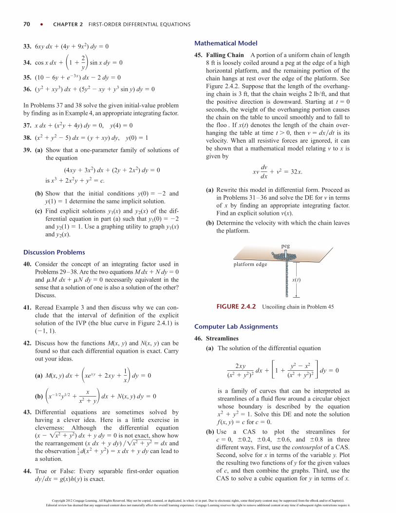
33. 6xy dx (4y 9x2) dy 0
34.
35. (10 6y e3x) dx 2 dy 0
36. (y2 xy3) dx (5y2 xy y3 sin y) dy 0
In Problems 37 and 38 solve the given initial-value problemby finding as in Example 4, an appropriate integrating factor.
37. x dx (x2y 4y) dy 0, y(4) 0
38. (x2 y2 5) dx (y xy) dy, y(0) 1
39. (a) Show that a one-parameter family of solutions ofthe equation
(4xy 3x2) dx (2y 2x2) dy 0
is x3 2x2y y2 c.
(b) Show that the initial conditions y(0) 2 and y(1) 1 determine the same implicit solution.
(c) Find explicit solutions y1(x) and y2(x) of the dif-ferential equation in part (a) such that y1(0) 2and y2(1) 1. Use a graphing utility to graph y1(x)and y2(x).
Discussion Problems
40. Consider the concept of an integrating factor used inProblems 29–38. Are the two equations M dx N dy 0and M dx N dy 0 necessarily equivalent in thesense that a solution of one is also a solution of the other?Discuss.
41. Reread Example 3 and then discuss why we can con-clude that the interval of definition of the explicitsolution of the IVP (the blue curve in Figure 2.4.1) is(1, 1).
42. Discuss how the functions M(x, y) and N(x, y) can befound so that each differential equation is exact. Carryout your ideas.
(a)
(b)
43. Differential equations are sometimes solved byhaving a clever idea. Here is a little exercise incleverness: Although the differential equation (x ) dx y dy 0 is not exact, show howthe rearrangement (x dx y dy) dx andthe observation d(x2 y2) x dx y dy can lead toa solution.
44. True or False: Every separable first-order equationdydx g(x)h(y) is exact.
12
1x2 y21x2 y2
x1/2y1/2 x
x2 y dx N(x, y) dy 0
M(x, y) dx xexy 2xy 1
x dy 0
cos x dx 1 2
y sin x dy 0
Mathematical Model
45. Falling Chain A portion of a uniform chain of length8 ft is loosely coiled around a peg at the edge of a highhorizontal platform, and the remaining portion of thechain hangs at rest over the edge of the platform. SeeFigure 2.4.2. Suppose that the length of the overhang-ing chain is 3 ft, that the chain weighs 2 lb/ft, and thatthe positive direction is downward. Starting at t 0seconds, the weight of the overhanging portion causesthe chain on the table to uncoil smoothly and to fall tothe floo . If x(t) denotes the length of the chain over-hanging the table at time t 0, then v dxdt is itsvelocity. When all resistive forces are ignored, it canbe shown that a mathematical model relating v to x isgiven by
.
(a) Rewrite this model in differential form. Proceed asin Problems 31–36 and solve the DE for v in termsof x by finding an appropriate integrating factor.Find an explicit solution v(x).
(b) Determine the velocity with which the chain leavesthe platform.
xv dv
dx v2 32x
70 CHAPTER 2 FIRST-ORDER DIFFERENTIAL EQUATIONS
x(t)
platform edge
peg
FIGURE 2.4.2 Uncoiling chain in Problem 45
Computer Lab Assignments
46. Streamlines
(a) The solution of the differential equation
is a family of curves that can be interpreted asstreamlines of a fluid flow around a circular objectwhose boundary is described by the equationx2 y2 1. Solve this DE and note the solutionf (x, y) c for c 0.
(b) Use a CAS to plot the streamlines forc 0, 0.2, 0.4, 0.6, and 0.8 in threedifferent ways. First, use the contourplot of a CAS.Second, solve for x in terms of the variable y. Plotthe resulting two functions of y for the given valuesof c, and then combine the graphs. Third, use theCAS to solve a cubic equation for y in terms of x.
2xy
(x2 y2)2 dx 1 y2 x2
(x2 y2)2 dy 0
Copyright 2012 Cengage Learning. All Rights Reserved. May not be copied, scanned, or duplicated, in whole or in part. Due to electronic rights, some third party content may be suppressed from the eBook and/or eChapter(s).
Editorial review has deemed that any suppressed content does not materially affect the overall learning experience. Cengage Learning reserves the right to remove additional content at any time if subsequent rights restrictions require it.

2.5 SOLUTIONS BY SUBSTITUTIONS 71
SOLUTIONS BY SUBSTITUTIONS
REVIEW MATERIAL Techniques of integration Separation of variables Solution of linear DEs
INTRODUCTION We usually solve a differential equation by recognizing it as a certain kind ofequation (say, separable, linear, or exact) and then carrying out a procedure, consisting of equation-specific mathematical steps, that yields a solution of the equation. But it is not uncommon to bestumped by a differential equation because it does not fall into one of the classes of equations thatwe know how to solve. The procedures that are discussed in this section may be helpful in thissituation.
2.5
Substitutions Often the first step in solving a differential equation consistsof transforming it into another differential equation by means of a substitution.For example, suppose we wish to transform the first-order differential equationdydx f (x, y) by the substitution y g(x, u), where u is regarded as a function ofthe variable x. If g possesses first-partial derivatives, then the Chain Rul
.
If we replace dydx by the foregoing derivative and replace y in f (x, y) by g(x, u), then
the DE dydx f (x, y) becomes gx(x, u) gu(x, u) f (x, g(x, u)), which, solved
for dudx, has the form F(x, u). If we can determine a solution u (x) of this
last equation, then a solution of the original differential equation is y g(x, (x)).In the discussion that follows we examine three different kinds of first-orde
differential equations that are solvable by means of a substitution.
Homogeneous Equations If a function f possesses the property f (tx, ty)
du
dx
du
dx
dy
dx
g
x dx
dx
g
u du
dxgives
dy
dx gx(x, u) gu(x, u)
du
dx
t f (x, y) for some real number , then f is said to be a homogeneous function ofdegree . For example, f (x, y) x3 y3 is a homogeneous function of degree 3,since
f (tx, ty) (tx)3 (ty)3 t3(x3 y3) t3f (x, y),
whereas f (x, y) x3 y3 1 is not homogeneous. A first-order DE in differentialform
M(x, y) dx N(x, y) dy 0 (1)
is said to be homogeneous* if both coefficient functions M and N are homogeneousfunctions of the same degree. In other words, (1) is homogeneous if
.
In addition, if M and N are homogeneous functions of degree , we can also write
, (2)M(x, y) xM(1, u) and N(x, y) xN(1, u), where u y>xM(tx, ty) tM(x, y) and N(tx, ty) tN(x, y)
*Here the word homogeneous does not mean the same as it did in the Remarks at the end of Section 2.3.Recall that a linear first-order equation a1(x)y a0(x)y g(x) is homogeneous when g(x) 0.
Copyright 2012 Cengage Learning. All Rights Reserved. May not be copied, scanned, or duplicated, in whole or in part. Due to electronic rights, some third party content may be suppressed from the eBook and/or eChapter(s).
Editorial review has deemed that any suppressed content does not materially affect the overall learning experience. Cengage Learning reserves the right to remove additional content at any time if subsequent rights restrictions require it.

72 CHAPTER 2 FIRST-ORDER DIFFERENTIAL EQUATIONS
and
. (3)
See Problem 31 in Exercises 2.5. Properties (2) and (3) suggest the substitutions that canbe used to solve a homogeneous differential equation. Specificall , either of the substi-tutions y ux or x vy, where u and v are new dependent variables, will reduce ahomogeneous equation to a separable first-orde differential equation. To show this, ob-serve that as a consequence of (2) a homogeneous equation M(x, y) dx N(x, y) dy 0can be rewritten as
,
where u yx or y ux. By substituting the differential dy u dx x du into thelast equation and gathering terms, we obtain a separable DE in the variables u and x:
or .
At this point we offer the same advice as in the preceding sections: Do not memorizeanything here (especially the last formula); rather, work through the procedure eachtime. The proof that the substitutions x vy and dx v dy y dv also lead to aseparable equation follows in an analogous manner from (3).
dx
x
N(1, u) du
M(1, u) uN(1, u) 0
[M(1, u) uN(1, u)] dx xN(1, u) du 0
M(1, u) dx N(1, u)[u dx x du] 0
xM(1, u) dx xN(1, u) dy 0 or M(1, u) dx N(1, u) dy 0
M(x, y) yM(v, 1) and N(x, y) yN(v, 1), where v x>y
EXAMPLE 1 Solving a Homogeneous DE
Solve (x2 y2) dx (x2 xy) dy 0.
SOLUTION Inspection of M(x, y) x2 y2 and N(x, y) x2 xy shows thatthese coefficients are homogeneous functions of degree 2. If we let y ux, thendy u dx x du, so after substituting, the given equation becomes
.
After integration the last line gives
.
Using the properties of logarithms, we can write the preceding solution as
.
Although either of the indicated substitutions can be used for every homoge-neous differential equation, in practice we try x vy whenever the function M(x, y)is simpler than N(x, y). Also it could happen that after using one substitution, we mayencounter integrals that are difficult or impossible to evaluate in closed form; switch-ing substitutions may result in an easier problem.
ln (x y)2
cx y
xor (x y)2 cxey/x
y
x 2 ln 1
y
x ln x lnc
u 2 ln 1 u ln x ln c
1 2
1 u du dx
x 0
1 u
1 u du
dx
x 0
x2 (1 u) dx x3(1 u) du 0
(x2 u2x2) dx (x2 ux2)[u dx x du] 0
; long division
; resubstituting u yx
Copyright 2012 Cengage Learning. All Rights Reserved. May not be copied, scanned, or duplicated, in whole or in part. Due to electronic rights, some third party content may be suppressed from the eBook and/or eChapter(s).
Editorial review has deemed that any suppressed content does not materially affect the overall learning experience. Cengage Learning reserves the right to remove additional content at any time if subsequent rights restrictions require it.

Bernoulli’s Equation The differential equation
, (4)
where n is any real number, is called Bernoulli’s equation. Note that for n 0 andn 1, equation (4) is linear. For n 0 and n 1 the substitution u y1n reducesany equation of form (4) to a linear equation.
dy
dx P(x)y f (x)yn
2.5 SOLUTIONS BY SUBSTITUTIONS 73
EXAMPLE 2 Solving a Bernoulli DE
Solve
SOLUTION We first rewrite the equation a
by dividing by x. With n 2 we have u y1 or y u1. We then substitute
into the given equation and simplify. The result is
.
The integrating factor for this linear equation on, say, (0, ) is
.
Integrating
gives x1u x c or u x2 cx. Since u y1, we have y 1u, so a solu-tion of the given equation is y 1(x2 cx).
Note that we have not obtained the general solution of the original nonlinear dif-ferential equation in Example 2, since y 0 is a singular solution of the equation.
Reduction to Separation of Variables A differential equation of the form
(5)
can always be reduced to an equation with separable variables by means of the sub-stitution u Ax By C, B 0. Example 3 illustrates the technique.
dy
dx f (Ax By C)
d
dx [x1u] 1
edx/x eln x eln x1 x1
du
dx
1
x u x
dy
dx
dy
du du
dx u2
du
dx
dy
dx
1
x y xy2
x dy
dx y x2y2.
; Chain Rule
EXAMPLE 3 An Initial-Value Problem
Solve
SOLUTION If we let u 2x y, then dudx 2 dydx, so the differentialequation is transformed into
.du
dx 2 u2 7 or
du
dx u2 9
dy
dx (2x y)2 7, y(0) 0.
Copyright 2012 Cengage Learning. All Rights Reserved. May not be copied, scanned, or duplicated, in whole or in part. Due to electronic rights, some third party content may be suppressed from the eBook and/or eChapter(s).
Editorial review has deemed that any suppressed content does not materially affect the overall learning experience. Cengage Learning reserves the right to remove additional content at any time if subsequent rights restrictions require it.

; replace by ce6c1
x
y
FIGURE 2.5.1 Solutions of DE inExample 3
74 CHAPTER 2 FIRST-ORDER DIFFERENTIAL EQUATIONS
The last equation is separable. Using partial fractions
and then integrating yields
.
Solving the last equation for u and then resubstituting gives the solution
. (6)
Finally, applying the initial condition y(0) 0 to the last equation in (6) gives c 1. Figure 2.5.1, obtained with the aid of a graphing utility, shows the graph of
the particular solution in dark blue, along with the graphs of
some other members of the family of solutions (6).
y 2x 3(1 e6x)
1 e6x
u 3(1 ce6x)
1 ce6x or y 2x 3(1 ce6x)
1 ce6x
1
6 ln u 3
u 3 x c1 oru 3
u 3 e6x6c1 ce6x
du
(u 3)(u 3) dx or
1
6 1
u 3
1
u 3 du dx
EXERCISES 2.5 Answers to selected odd-numbered problems begin on page ANS-2.
Each DE in Problems 1–14 is homogeneous.
In Problems 1–10 solve the given differential equation byusing an appropriate substitution.
1. (x y) dx x dy 0 2. (x y) dx x dy 0
3. x dx (y 2x) dy 0 4. y dx 2(x y) dy
5. (y2 yx) dx x2 dy 0
6. (y2 yx) dx x2 dy 0
7.
8.
9.
10.
In Problems 11–14 solve the given initial-value problem.
11.
12.
13. (x yey/x) dx xey/x dy 0, y(1) 0
14. y dx x(ln x ln y 1) dy 0, y(1) e
(x2 2y2) dx
dy xy, y(1) 1
xy2 dy
dx y3 x3, y(1) 2
x dy
dx y 1x2 y2, x 0
y dx (x 1xy ) dy 0
dy
dx
x 3y
3x y
dy
dx
y x
y x
Each DE in Problems 15–22 is a Bernoulli equation.
In Problems 15–20 solve the given differential equation byusing an appropriate substitution.
15. 16.
17. 18.
19. 20.
In Problems 21 and 22 solve the given initial-value problem.
21.
22.
Each DE in Problems 23–30 is of the form given in (5).
In Problems 23–28 solve the given differential equation byusing an appropriate substitution.
23. 24.
25. 26.
27. 28.dy
dx 1 eyx5dy
dx 2 1y 2x 3
dy
dx sin(x y)
dy
dx tan2(x y)
dy
dx
1 x y
x y
dy
dx (x y 1)2
y1/2 dy
dx y3/2 1, y(0) 4
x2 dy
dx 2xy 3y4, y(1) 1
2
3(1 t2) dy
dt 2ty( y3 1)t2
dy
dt y2 ty
x dy
dx (1 x)y xy2dy
dx y (xy3 1)
dy
dx y exy2x
dy
dx y
1
y2
Copyright 2012 Cengage Learning. All Rights Reserved. May not be copied, scanned, or duplicated, in whole or in part. Due to electronic rights, some third party content may be suppressed from the eBook and/or eChapter(s).
Editorial review has deemed that any suppressed content does not materially affect the overall learning experience. Cengage Learning reserves the right to remove additional content at any time if subsequent rights restrictions require it.

2.6 A NUMERICAL METHOD 75
In Problems 29 and 30 solve the given initial-value problem.
29.
30.
Discussion Problems
31. Explain why it is always possible to express any homoge-neous differential equation M(x, y) dx N(x, y) dy 0 inthe form
.
You might start by proving that
.
32. Put the homogeneous differential equation
(5x2 2y2) dx xy dy 0
into the form given in Problem 31.
33. (a) Determine two singular solutions of the DE inProblem 10.
(b) If the initial condition y(5) 0 is as prescribed inProblem 10, then what is the largest interval I overwhich the solution is defined? Use a graphing util-ity to graph the solution curve for the IVP.
34. In Example 3 the solution y(x) becomes unbounded asx : . Nevertheless, y(x) is asymptotic to a curve asx : and to a different curve as x : . What are theequations of these curves?
35. The differential equation dydx P(x) Q(x)y R(x)y2
is known as Riccati’s equation.
(a) A Riccati equation can be solved by a successionof two substitutions provided that we know a
M(x, y) xaM(1, y>x) and N(x, y) xaN(1, y>x)
dy
dx F y
x
dy
dx
3x 2y
3x 2y 2, y (1) 1
dy
dx cos(x y), y(0) >4 particular solution y1 of the equation. Show that the
substitution y y1 u reduces Riccati’s equationto a Bernoulli equation (4) with n 2. TheBernoulli equation can then be reduced to a linearequation by the substitution w u1.
(b) Find a one-parameter family of solutions for thedifferential equation
where y1 2x is a known solution of the equation.
36. Determine an appropriate substitution to solve
xy y ln(xy).
Mathematical Models
37. Falling Chain In Problem 45 in Exercises 2.4 we sawthat a mathematical model for the velocity v of a chainslipping off the edge of a high horizontal platform is
.
In that problem you were asked to solve the DE by con-verting it into an exact equation using an integratingfactor. This time solve the DE using the fact that it is aBernoulli equation.
38. Population Growth In the study of population dy-namics one of the most famous models for a growingbut bounded population is the logistic equation
,
where a and b are positive constants. Although wewill come back to this equation and solve it by analternative method in Section 3.2, solve the DE thisfirst time using the fact that it is a Bernoulli equation.
dP
dt P(a bP)
xv dv
dx v2 32x
dy
dx 4
x2 1
x y y2
A NUMERICAL METHOD
INTRODUCTION A first-order differential equation dydx f (x, y) is a source of information.We started this chapter by observing that we could garner qualitative information from a first-ordeDE about its solutions even before we attempted to solve the equation. Then in Sections 2.2–2.5 weexamined first-order DEs analytically—that is, we developed some procedures for obtaining explicitand implicit solutions. But a differential equation can a possess a solution, yet we may not be ableto obtain it analytically. So to round out the picture of the different types of analyses of differentialequations, we conclude this chapter with a method by which we can “solve” the differential equa-tion numerically—this means that the DE is used as the cornerstone of an algorithm for approximat-ing the unknown solution.
In this section we are going to develop only the simplest of numerical methods—a method thatutilizes the idea that a tangent line can be used to approximate the values of a function in a smallneighborhood of the point of tangency. A more extensive treatment of numerical methods for ordi-nary differential equations is given in Chapter 9.
2.6
Copyright 2012 Cengage Learning. All Rights Reserved. May not be copied, scanned, or duplicated, in whole or in part. Due to electronic rights, some third party content may be suppressed from the eBook and/or eChapter(s).
Editorial review has deemed that any suppressed content does not materially affect the overall learning experience. Cengage Learning reserves the right to remove additional content at any time if subsequent rights restrictions require it.

76 CHAPTER 2 FIRST-ORDER DIFFERENTIAL EQUATIONS
Using the Tangent Line Let us assume that the first-order initial-valueproblem
(1)
possesses a solution. One way of approximating this solution is to use tangent lines.For example, let y(x) denote the unknown solution of the first-order initial-valueproblem The nonlinear differential equation inthis IVP cannot be solved directly by any of the methods considered in Sections 2.2,2.4, and 2.5; nevertheless, we can still find approximate numerical values of theunknown y(x). Specificall , suppose we wish to know the value of y(2.5). The IVPhas a solution, and as the flow of the direction field of the DE in Figure 2.6.1(a) sug-gests, a solution curve must have a shape similar to the curve shown in blue.
The direction field in Figure 2.6.1(a) was generated with lineal elements passingthrough points in a grid with integer coordinates. As the solution curve passesthrough the initial point (2, 4), the lineal element at this point is a tangent line withslope given by As is apparent in Figure 2.6.1(a)and the “zoom in” in Figure 2.6.1(b), when x is close to 2, the points on the solutioncurve are close to the points on the tangent line (the lineal element). Using the point(2, 4), the slope f (2, 4) 1.8, and the point-slope form of a line, we find that an equa-tion of the tangent line is y L(x), where L(x) 1.8x 0.4. This last equation,called a linearization of y(x) at x 2, can be used to approximate values of y(x)within a small neighborhood of x 2. If y1 L(x1) denotes the y-coordinate on thetangent line and y(x1) is the y-coordinate on the solution curve corresponding to anx-coordinate x1 that is close to x 2, then y(x1) y1. If we choose, say, x1 2.1,then y1 L(2.1) 1.8(2.1) 0.4 4.18, so y(2.1) 4.18.
f (2, 4) 0.114 0.4(2)2 1.8.
y 0.11y 0.4x2, y(2) 4.
y f (x, y), y(x0) y0
2
(2, 4) slope m =1.8
x
y
2
4
_2
(a) direction field for y 0 (b) lineal elementat (2, 4)
e solution curv
FIGURE 2.6.1 Magnification of a neighborhood about the point (2, 4
solution curv e
x
y
x1 = +x0 hx0
L(x)
(x0, y0)(x1, y1)
h
(x1, y(x1))
slope = f(x0, y0)
error
FIGURE 2.6.2 Approximating y(x1)using a tangent line
Euler’s Method To generalize the procedure just illustrated, we use the lin-
*This is not an actual tangent line, since (x1, y1) lies on the first tangent and not on the solution curve
earization of the unknown solution y(x) of (1) at x x0:
. (2)
The graph of this linearization is a straight line tangent to the graph of y y(x) atthe point (x0, y0). We now let h be a positive increment of the x-axis, as shown inFigure 2.6.2. Then by replacing x by x1 x0 h in (2), we get
,
where y1 L(x1). The point (x1, y1) on the tangent line is an approximation to thepoint (x1, y(x1)) on the solution curve. Of course, the accuracy of the approxima-tion L(x1) y(x1) or y1 y(x1) depends heavily on the size of the increment h.Usually, we must choose this step size to be “reasonably small.” We now repeat theprocess using a second “tangent line” at (x1, y1).* By identifying the new starting
L(x1) y0 f (x0, y0)(x0 h x0) or y1 y0 hf (x1, y1)
L(x) y0 f (x0, y0)(x x0)
Copyright 2012 Cengage Learning. All Rights Reserved. May not be copied, scanned, or duplicated, in whole or in part. Due to electronic rights, some third party content may be suppressed from the eBook and/or eChapter(s).
Editorial review has deemed that any suppressed content does not materially affect the overall learning experience. Cengage Learning reserves the right to remove additional content at any time if subsequent rights restrictions require it.
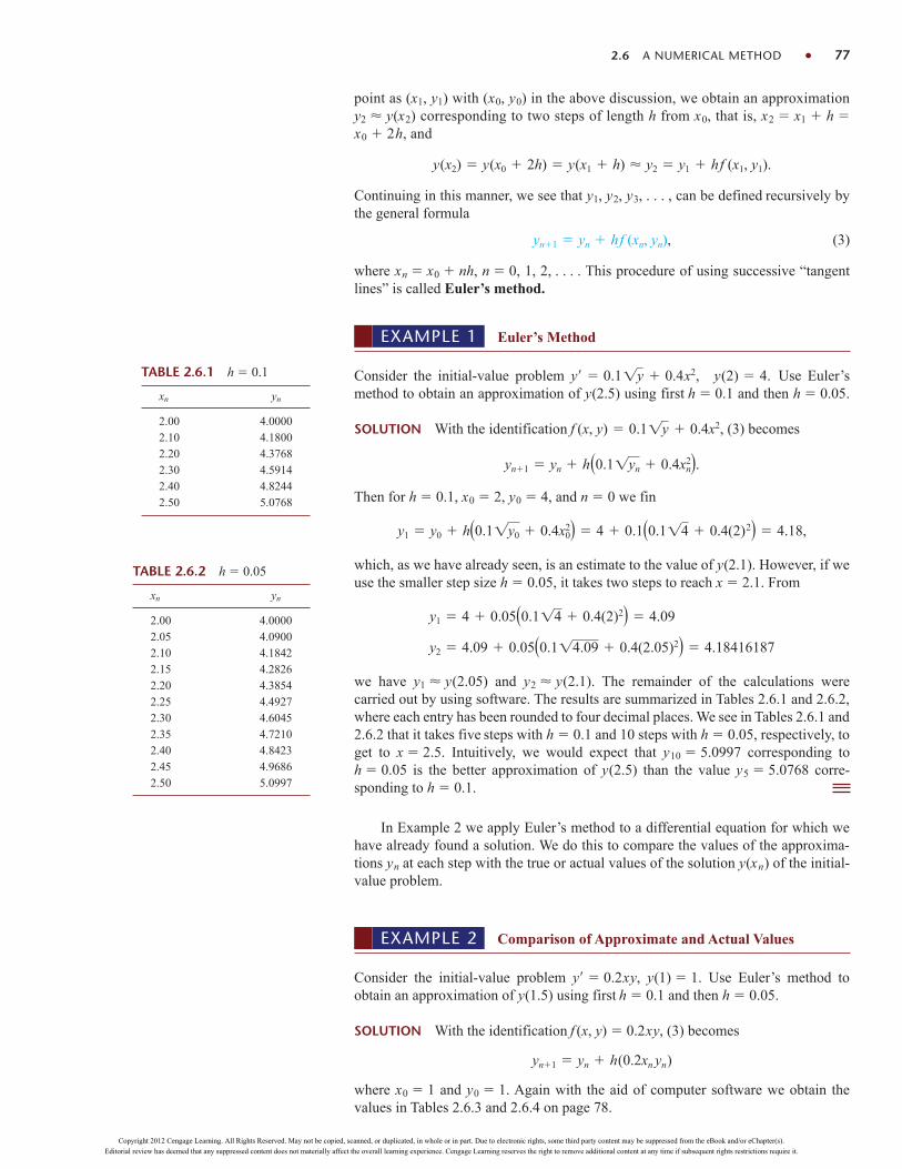
TABLE 2.6.1 h 0.1
xn yn
2.00 4.00002.10 4.18002.20 4.37682.30 4.59142.40 4.82442.50 5.0768
TABLE 2.6.2 h 0.05
xn yn
2.00 4.00002.05 4.09002.10 4.18422.15 4.28262.20 4.38542.25 4.49272.30 4.60452.35 4.72102.40 4.84232.45 4.96862.50 5.0997
2.6 A NUMERICAL METHOD 77
point as (x1, y1) with (x0, y0) in the above discussion, we obtain an approximation y2 y(x2) corresponding to two steps of length h from x0, that is, x2 x1 h x0 2h, and
.
Continuing in this manner, we see that y1, y2, y3, . . . , can be defined recursively bythe general formula
, (3)
where xn x0 nh, n 0, 1, 2, . . . . This procedure of using successive “tangentlines” is called Euler’s method.
yn1 yn hf (xn, yn)
y(x2) y(x0 2h) y(x1 h) y2 y1 hf (x1, y1)
EXAMPLE 1 Euler’s Method
Consider the initial-value problem Use Euler’smethod to obtain an approximation of y(2.5) using first h 0.1 and then h 0.05.
SOLUTION With the identification (3) becomes
.
Then for h 0.1, x0 2, y0 4, and n 0 we fin
,
which, as we have already seen, is an estimate to the value of y(2.1). However, if weuse the smaller step size h 0.05, it takes two steps to reach x 2.1. From
we have y1 y(2.05) and y2 y(2.1). The remainder of the calculations werecarried out by using software. The results are summarized in Tables 2.6.1 and 2.6.2,where each entry has been rounded to four decimal places. We see in Tables 2.6.1 and2.6.2 that it takes five steps with h 0.1 and 10 steps with h 0.05, respectively, toget to x 2.5. Intuitively, we would expect that y10 5.0997 corresponding toh 0.05 is the better approximation of y(2.5) than the value y5 5.0768 corre-sponding to h 0.1.
In Example 2 we apply Euler’s method to a differential equation for which wehave already found a solution. We do this to compare the values of the approxima-tions yn at each step with the true or actual values of the solution y(xn) of the initial-value problem.
y2 4.09 0.05(0.114.09 0.4(2.05)2) 4.18416187
y1 4 0.05(0.114 0.4(2)2) 4.09
y1 y0 h(0.11y0 0.4x02) 4 0.1(0.114 0.4(2)2) 4.18
yn1 yn h(0.11yn 0.4xn2)
f (x, y) 0.11y 0.4x2,
y 0.11y 0.4x2, y(2) 4.
EXAMPLE 2 Comparison of Approximate and Actual Values
Consider the initial-value problem y 0.2xy, y(1) 1. Use Euler’s method toobtain an approximation of y(1.5) using first h 0.1 and then h 0.05.
SOLUTION With the identification f (x, y) 0.2xy, (3) becomes
where x0 1 and y0 1. Again with the aid of computer software we obtain thevalues in Tables 2.6.3 and 2.6.4 on page 78.
yn1 yn h(0.2xn yn)
Copyright 2012 Cengage Learning. All Rights Reserved. May not be copied, scanned, or duplicated, in whole or in part. Due to electronic rights, some third party content may be suppressed from the eBook and/or eChapter(s).
Editorial review has deemed that any suppressed content does not materially affect the overall learning experience. Cengage Learning reserves the right to remove additional content at any time if subsequent rights restrictions require it.

78 CHAPTER 2 FIRST-ORDER DIFFERENTIAL EQUATIONS
In Example 1 the true or actual values were calculated from the known solution(Verify.) The absolute error is defined to b
.
The relative error and percentage relative error are, in turn,
.
It is apparent from Tables 2.6.3 and 2.6.4 that the accuracy of the approximationsimproves as the step size h decreases. Also, we see that even though the percentagerelative error is growing with each step, it does not appear to be that bad. But youshould not be deceived by one example. If we simply change the coefficient of theright side of the DE in Example 2 from 0.2 to 2, then at xn 1.5 the percentagerelative errors increase dramatically. See Problem 4 in Exercises 2.6.
A Caveat Euler’s method is just one of many different ways in which a solu-tion of a differential equation can be approximated. Although attractive for its sim-plicity, Euler’s method is seldom used in serious calculations. It was introducedhere simply to give you a first taste of numerical methods. We will go into greaterdetail in discussing numerical methods that give significantly greater accuracy, no-tably the fourth order Runge-Kutta method, referred to as the RK4 method, inChapter 9.
Numerical Solvers Regardless of whether we can actually fin an explicitor implicit solution, if a solution of a differential equation exists, it represents asmooth curve in the Cartesian plane. The basic idea behind any numerical methodfor first-orde ordinary differential equations is to somehow approximate they-values of a solution for preselected values of x. We start at a specifie initial point(x0, y0) on a solution curve and proceed to calculate in a step-by-step fashion asequence of points (x1, y1), (x2, y2), . . . , (xn, yn) whose y-coordinates yi approxi-mate the y-coordinates y(xi) of points (x1, y(x1)), (x2, y(x2)), . . . , (xn, y(xn)) that lieon the graph of the usually unknown solution y(x). By taking the x-coordinatesclose together (that is, for small values of h) and by joining the points (x1, y1),(x2, y2), . . . , (xn, yn) with short line segments, we obtain a polygonal curve whosequalitative characteristics we hope are close to those of an actual solution curve.Drawing curves is something that is well suited to a computer. A computer programwritten to either implement a numerical method or render a visual representation ofan approximate solution curve fittin the numerical data produced by this methodis referred to as a numerical solver. Many different numerical solvers are commer-cially available, either embedded in a larger software package, such as a computer
absolute error
actual value and
absolute error
actual value 100
actual value approximation
y e0.1(x21).
TABLE 2.6.3 h 0.1
xn yn Actual value Abs. error % Rel. error
1.00 1.0000 1.0000 0.0000 0.001.10 1.0200 1.0212 0.0012 0.121.20 1.0424 1.0450 0.0025 0.241.30 1.0675 1.0714 0.0040 0.371.40 1.0952 1.1008 0.0055 0.501.50 1.1259 1.1331 0.0073 0.64
TABLE 2.6.4 h 0.05
xn yn Actual value Abs. error % Rel. error
1.00 1.0000 1.0000 0.0000 0.001.05 1.0100 1.0103 0.0003 0.031.10 1.0206 1.0212 0.0006 0.061.15 1.0318 1.0328 0.0009 0.091.20 1.0437 1.0450 0.0013 0.121.25 1.0562 1.0579 0.0016 0.161.30 1.0694 1.0714 0.0020 0.191.35 1.0833 1.0857 0.0024 0.221.40 1.0980 1.1008 0.0028 0.251.45 1.1133 1.1166 0.0032 0.291.50 1.1295 1.1331 0.0037 0.32
Copyright 2012 Cengage Learning. All Rights Reserved. May not be copied, scanned, or duplicated, in whole or in part. Due to electronic rights, some third party content may be suppressed from the eBook and/or eChapter(s).
Editorial review has deemed that any suppressed content does not materially affect the overall learning experience. Cengage Learning reserves the right to remove additional content at any time if subsequent rights restrictions require it.
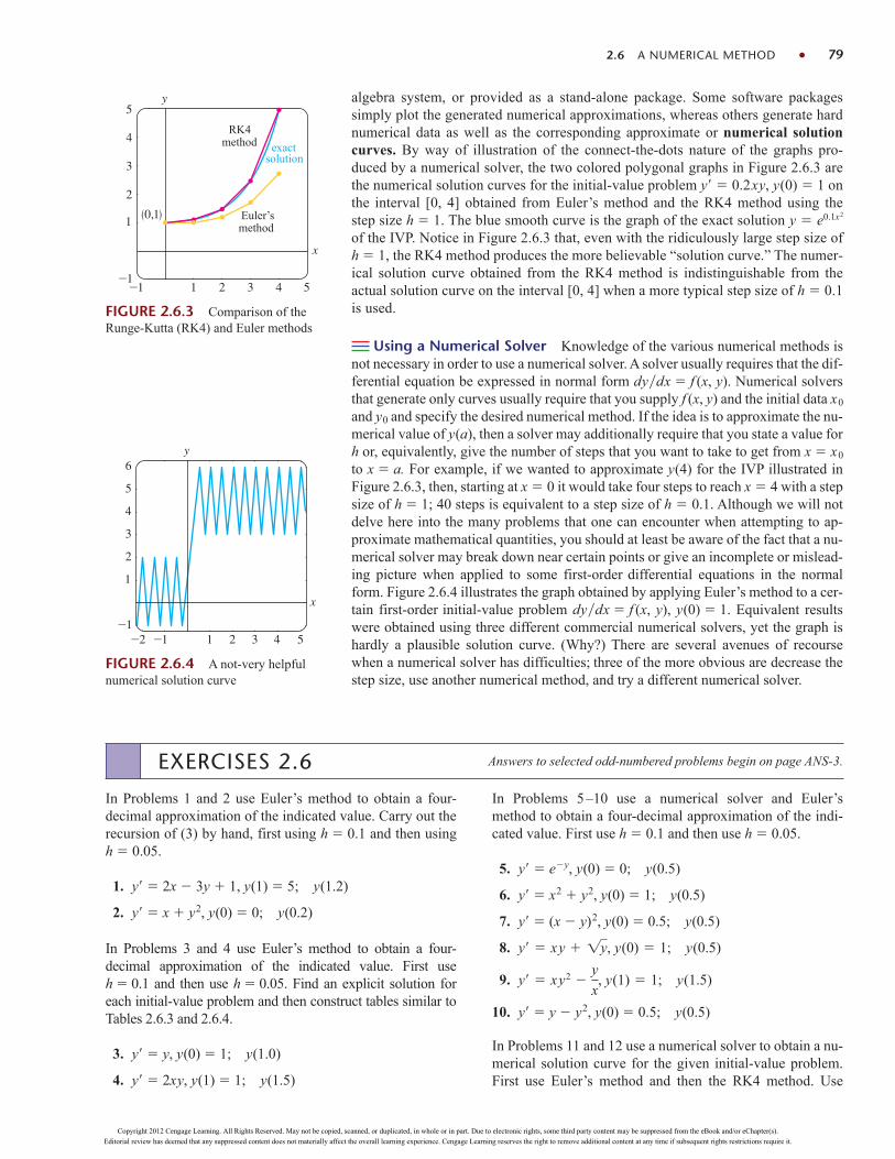
algebra system, or provided as a stand-alone package. Some software packagessimply plot the generated numerical approximations, whereas others generate hardnumerical data as well as the corresponding approximate or numerical solutioncurves. By way of illustration of the connect-the-dots nature of the graphs pro-duced by a numerical solver, the two colored polygonal graphs in Figure 2.6.3 arethe numerical solution curves for the initial-value problem y 0.2xy, y(0) 1 onthe interval [0, 4] obtained from Euler’s method and the RK4 method using thestep size h 1. The blue smooth curve is the graph of the exact solutionof the IVP. Notice in Figure 2.6.3 that, even with the ridiculously large step size ofh 1, the RK4 method produces the more believable “solution curve.” The numer-ical solution curve obtained from the RK4 method is indistinguishable from theactual solution curve on the interval [0, 4] when a more typical step size of h 0.1is used.
Using a Numerical Solver Knowledge of the various numerical methods isnot necessary in order to use a numerical solver. A solver usually requires that the dif-ferential equation be expressed in normal form dydx f (x, y). Numerical solversthat generate only curves usually require that you supply f (x, y) and the initial data x0
and y0 and specify the desired numerical method. If the idea is to approximate the nu-merical value of y(a), then a solver may additionally require that you state a value forh or, equivalently, give the number of steps that you want to take to get from x x0
to x a. For example, if we wanted to approximate y(4) for the IVP illustrated inFigure 2.6.3, then, starting at x 0 it would take four steps to reach x 4 with a stepsize of h 1; 40 steps is equivalent to a step size of h 0.1. Although we will notdelve here into the many problems that one can encounter when attempting to ap-proximate mathematical quantities, you should at least be aware of the fact that a nu-merical solver may break down near certain points or give an incomplete or mislead-ing picture when applied to some first-order differential equations in the normalform. Figure 2.6.4 illustrates the graph obtained by applying Euler’s method to a cer-tain first-order initial-value problem dydx f (x, y), y(0) 1. Equivalent resultswere obtained using three different commercial numerical solvers, yet the graph ishardly a plausible solution curve. (Why?) There are several avenues of recoursewhen a numerical solver has difficulties; three of the more obvious are decrease thestep size, use another numerical method, and try a different numerical solver.
y e0.1x2
FIGURE 2.6.4 A not-very helpfulnumerical solution curve
x
y
1 2 3 4 5_1
123456
_2 _1
2.6 A NUMERICAL METHOD 79
exact solution
(0,1) Euler’smethod
RK4method
_1 1 2 3 4 5
y
x
4
5
3
2
1
_1
FIGURE 2.6.3 Comparison of theRunge-Kutta (RK4) and Euler methods
EXERCISES 2.6 Answers to selected odd-numbered problems begin on page ANS-3.
In Problems 1 and 2 use Euler’s method to obtain a four-decimal approximation of the indicated value. Carry out therecursion of (3) by hand, first using h 0.1 and then usingh 0.05.
1. y 2x 3y 1, y(1) 5; y(1.2)
2. y x y2, y(0) 0; y(0.2)
In Problems 3 and 4 use Euler’s method to obtain a four-decimal approximation of the indicated value. First use h 0.1 and then use h 0.05. Find an explicit solution foreach initial-value problem and then construct tables similar toTables 2.6.3 and 2.6.4.
3. y y, y(0) 1; y(1.0)
4. y 2xy, y(1) 1; y(1.5)
In Problems 5–10 use a numerical solver and Euler’smethod to obtain a four-decimal approximation of the indi-cated value. First use h 0.1 and then use h 0.05.
5. y ey, y(0) 0; y(0.5)
6. y x2 y2, y(0) 1; y(0.5)
7. y (x y)2, y(0) 0.5; y(0.5)
8.
9.
10. y y y2, y(0) 0.5; y(0.5)
In Problems 11 and 12 use a numerical solver to obtain a nu-merical solution curve for the given initial-value problem.First use Euler’s method and then the RK4 method. Use
y xy2 y
x, y(1) 1; y(1.5)
y xy 1y, y(0) 1; y(0.5)
Copyright 2012 Cengage Learning. All Rights Reserved. May not be copied, scanned, or duplicated, in whole or in part. Due to electronic rights, some third party content may be suppressed from the eBook and/or eChapter(s).
Editorial review has deemed that any suppressed content does not materially affect the overall learning experience. Cengage Learning reserves the right to remove additional content at any time if subsequent rights restrictions require it.
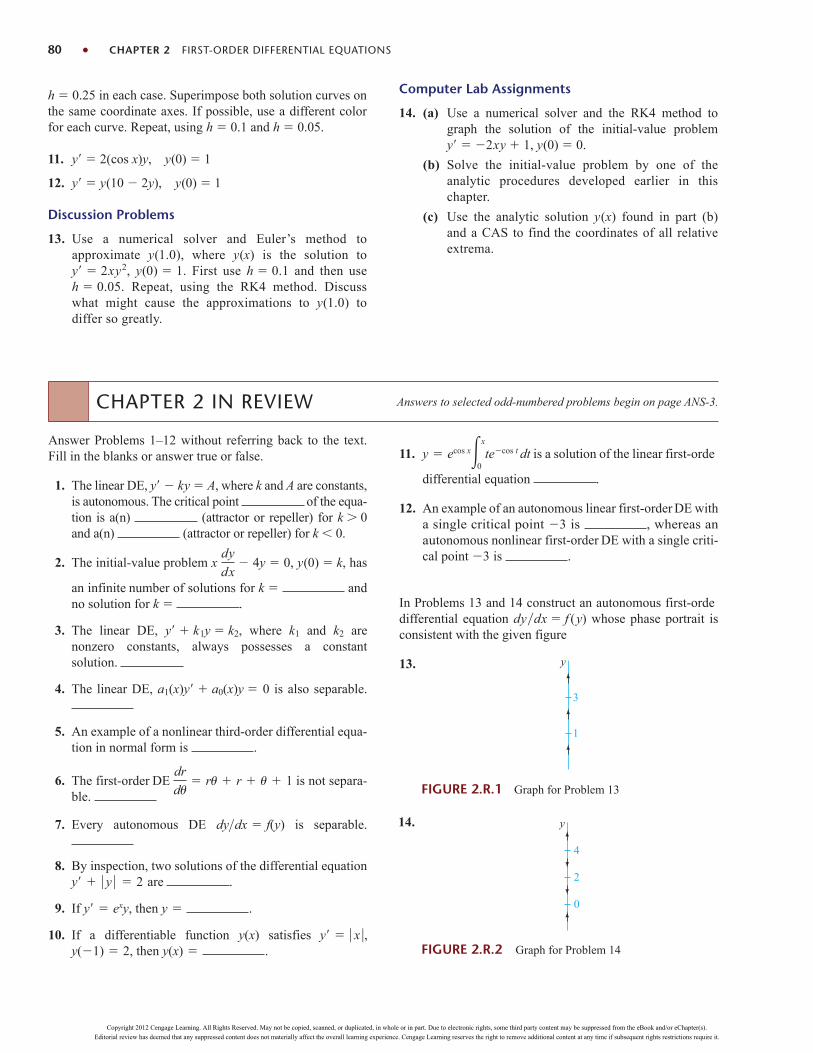
80 CHAPTER 2 FIRST-ORDER DIFFERENTIAL EQUATIONS
h 0.25 in each case. Superimpose both solution curves onthe same coordinate axes. If possible, use a different colorfor each curve. Repeat, using h 0.1 and h 0.05.
11. y 2(cos x)y, y(0) 1
12. y y(10 2y), y(0) 1
Discussion Problems
13. Use a numerical solver and Euler’s method toapproximate y(1.0), where y(x) is the solution toy 2xy2, y(0) 1. First use h 0.1 and then use h 0.05. Repeat, using the RK4 method. Discusswhat might cause the approximations to y(1.0) todiffer so greatly.
Computer Lab Assignments
14. (a) Use a numerical solver and the RK4 method tograph the solution of the initial-value problemy 2xy 1, y(0) 0.
(b) Solve the initial-value problem by one of theanalytic procedures developed earlier in thischapter.
(c) Use the analytic solution y(x) found in part (b)and a CAS to find the coordinates of all relativeextrema.
CHAPTER 2 IN REVIEW Answers to selected odd-numbered problems begin on page ANS-3.
Answer Problems 1–12 without referring back to the text.Fill in the blanks or answer true or false.
1. The linear DE, y ky A, where k and A are constants,is autonomous. The critical point of the equa-tion is a(n) (attractor or repeller) for k 0and a(n) (attractor or repeller) for k 0.
2. The initial-value problem x 4y 0, y(0) k, has
an infinite number of solutions for k andno solution for k .
3. The linear DE, y k1y k2, where k1 and k2 arenonzero constants, always possesses a constant solution.
4. The linear DE, a1(x)y a0(x)y 0 is also separable.
5. An example of a nonlinear third-order differential equa-tion in normal form is .
6. The first-order DE is not separa-ble.
7. Every autonomous DE is separable.
8. By inspection, two solutions of the differential equationare .
9. If then .
10. If a differentiable function satisfiesthen .y(x) y(1) 2,
y x ,y(x)
y y exy,
y y 2
dy>dx f(y)
dr
du ru r u 1
dy
dx
11. is a solution of the linear first-orde
differential equation .
12. An example of an autonomous linear first-order DE witha single critical point is , whereas anautonomous nonlinear first-order DE with a single criti-cal point is .
In Problems 13 and 14 construct an autonomous first-ordedifferential equation dydx f (y) whose phase portrait isconsistent with the given figure
13.
3
3
y ecos xx
0tecos t dt
1
3
y
FIGURE 2.R.1 Graph for Problem 13
14.
0
2
4
y
FIGURE 2.R.2 Graph for Problem 14
Copyright 2012 Cengage Learning. All Rights Reserved. May not be copied, scanned, or duplicated, in whole or in part. Due to electronic rights, some third party content may be suppressed from the eBook and/or eChapter(s).
Editorial review has deemed that any suppressed content does not materially affect the overall learning experience. Cengage Learning reserves the right to remove additional content at any time if subsequent rights restrictions require it.

CHAPTER 2 IN REVIEW 81
15. The number 0 is a critical point of the autonomous dif-ferential equation dxdt xn, where n is a positive in-teger. For what values of n is 0 asymptotically stable?Semi-stable? Unstable? Repeat for the differential equa-tion dxdt xn.
16. Consider the differential equation
The function f (P) has one real zero, as shown inFigure 2.R.3. Without attempting to solve the differen-tial equation, estimate the value of lim t: P(t).
f (P) 0.5P 3 1.7P 3.4.
dP>dt f (P), where
(g) y dx (y xy2) dy (h)
(i) xy y y2 2x ( j) 2xy y y2 2x2
(k) y dx x dy 0
(l)
(m) (n)
In Problems 19–26 solve the given differential equation.
19. (y2 1) dx y sec2 x dy
20. y(ln x ln y) dx (x ln x x ln y y) dy
21.
22.
23.
24. (2x y 1)y 1
25. (x2 4) dy (2x 8xy) dx
26. (2r2 cos sin r cos ) d (4r sin 2r cos2 ) dr 0
In Problems 27 and 28 solve the given initial-value problemand give the largest interval I on which the solution is defined
27.
28.
29. (a) Without solving, explain why the initial-valueproblem
has no solution for y0 0.(b) Solve the initial-value problem in part (a) for
y0 0 and find the largest interval I on which thesolution is defined
30. (a) Find an implicit solution of the initial-value problem
.
(b) Find an explicit solution of the problem in part (a) andgive the largest interval I over which the solution isdefined.A graphing utility may be helpful here.
dy
dx
y2 x2
xy, y(1) 12
dy
dx 1y, y(x0) y0
dy
dt 2(t 1)y2 0, y(0) 1
8
sin xdy
dx (cos x)y 0, y (7p>6) 2
tdQ
dt Q t 4 ln t
dx
dy 4y2 6xy
3y2 2x
(6x 1)y2 dy
dx 3x2 2y3 0
y
x2
dy
dx e2x3y2
0dy
dx
x
y
y
x 1
x2 2y
x dx (3 ln x2) dy
xdy
dx yex/y x
FIGURE 2.R.4 Portion of a direction field for Problem 1
P1
1
f
FIGURE 2.R.3 Graph for Problem 16
17. Figure 2.R.4 is a portion of a direction field of a differ-ential equation dydx f (x, y). By hand, sketch twodifferent solution curves—one that is tangent to the lin-eal element shown in black and one that is tangent to thelineal element shown in red.
18. Classify each differential equation as separable, exact,linear, homogeneous, or Bernoulli. Some equations maybe more than one kind. Do not solve.
(a) (b)
(c) (d)
(e) (f)dy
dx 5y y2dy
dx
y2 y
x2 x
dy
dx
1
x(x y)(x 1)
dy
dx y 10
dy
dx
1
y x
dy
dx
x y
x
Copyright 2012 Cengage Learning. All Rights Reserved. May not be copied, scanned, or duplicated, in whole or in part. Due to electronic rights, some third party content may be suppressed from the eBook and/or eChapter(s).
Editorial review has deemed that any suppressed content does not materially affect the overall learning experience. Cengage Learning reserves the right to remove additional content at any time if subsequent rights restrictions require it.

integers, 7 m 7, 7 n 7. In each direction fieldsketch by hand an approximate solution curve that passesthrough each of the solid points shown in red. Discuss: Doesit appear that the DE possesses critical points in the interval3.5 y 3.5? If so, classify the critical points as asymp-totically stable, unstable, or semi-stable.
x
321_1_2_3
_3_2_1
123
y
FIGURE 2.R.6 Portion of a direction field for Problem 3
x
y
FIGURE 2.R.5 Graph for Problem 3134.
FIGURE 2.R.7 Portion of a direction field for Problem 3
x
321_1_2_3
_3_2_1
123
y
82 CHAPTER 2 FIRST-ORDER DIFFERENTIAL EQUATIONS
31. Graphs of some members of a family of solutions for afirst-orde differential equation dydx f (x, y) areshown in Figure 2.R.5. The graphs of two implicitsolutions, one that passes through the point (1, 1) andone that passes through (1, 3), are shown in blue.Reproduce the figur on a piece of paper. With coloredpencils trace out the solution curves for the solutionsy y1(x) and y y2(x) define by the implicit solu-tions such that y1(1) 1 and y2(1) 3, respectively.Estimate the intervals on which the solutions y y1(x)and y y2(x) are defined
32. Use Euler’s method with step size h 0.1 to approxi-mate y(1.2), where y(x) is a solution of the initial-valueproblem , y(1) 9.
In Problems 33 and 34 each figure represents a portion of adirection field of an autonomous first-order differential equa-tion dydx f (y). Reproduce the figure on a separate pieceof paper and then complete the direction field over the grid.The points of the grid are (mh, nh), where m and nh 1
2,
y 1 x1y
33.
Copyright 2012 Cengage Learning. All Rights Reserved. May not be copied, scanned, or duplicated, in whole or in part. Due to electronic rights, some third party content may be suppressed from the eBook and/or eChapter(s).
Editorial review has deemed that any suppressed content does not materially affect the overall learning experience. Cengage Learning reserves the right to remove additional content at any time if subsequent rights restrictions require it.

83
3 Modeling with First-Order Differential Equations
3.1 Linear Models
3.2 Nonlinear Models
3.3 Modeling with Systems of First-Order DEs
Chapter 3 in Review
In Section 1.3 we saw how a first-order di ferential equation could be used as a
mathematical model in the study of population growth, radioactive decay,
continuous compound interest, cooling of bodies, mixtures, chemical reactions,
fluid draining from a tank, velocity of a falling bod , and current in a series circuit.
Using the methods of Chapter 2, we are now able to solve some of the linear DEs in
Section 3.1 and nonlinear DEs in Section 3.2 that commonly appear in applications.
The chapter concludes with the natural next step. In Section 3.3 we examine how
systems of first-order di ferential equations can arise as mathematical models in
coupled physical systems (for example, electrical networks, and a population of
predators such as foxes interacting with a population of prey such as rabbits).
Copyright 2012 Cengage Learning. All Rights Reserved. May not be copied, scanned, or duplicated, in whole or in part. Due to electronic rights, some third party content may be suppressed from the eBook and/or eChapter(s).
Editorial review has deemed that any suppressed content does not materially affect the overall learning experience. Cengage Learning reserves the right to remove additional content at any time if subsequent rights restrictions require it.

84 CHAPTER 3 MODELING WITH FIRST-ORDER DIFFERENTIAL EQUATIONS
Growth and Decay The initial-value problem
, (1)
where k is a constant of proportionality, serves as a model for diverse phenomenainvolving either growth or decay. We saw in Section 1.3 that in biological applica-tions the rate of growth of certain populations (bacteria, small animals) over shortperiods of time is proportional to the population present at time t. Knowing the pop-ulation at some arbitrary initial time t0, we can then use the solution of (1) to predictthe population in the future—that is, at times t t0. The constant of proportional-ity k in (1) can be determined from the solution of the initial-value problem, using asubsequent measurement of x at a time t1 t0. In physics and chemistry (1) is seenin the form of a first-o der reaction —that is, a reaction whose rate, or velocity,dxdt is directly proportional to the amount x of a substance that is unconvertedor remaining at time t. The decomposition, or decay, of U-238 (uranium) byradioactivity into Th-234 (thorium) is a first-order reaction
EXAMPLE 1 Bacterial Growth
A culture initially has P0 number of bacteria. At t 1 h the number of bacteria is mea-sured to be . If the rate of growth is proportional to the number of bacteria P(t) pre-sent at time t, determine the time necessary for the number of bacteria to triple.
SOLUTION We first solve the differential equation in (1), with the symbol x replacedby P. With t0 0 the initial condition is P(0) P0. We then use the empirical obser-vation that to determine the constant of proportionality k.
Notice that the differential equation dPdt kP is both separable and linear.When it is put in the standard form of a linear first-order DE
,
we can see by inspection that the integrating factor is ekt. Multiplying both sides ofthe equation by this term and integrating gives, in turn,
.
Therefore P(t) cekt. At t 0 it follows that P0 ce0 c, so P(t) P0ekt. At t 1 we have or . From the last equation we get
, so P(t) P0e0.4055t. To find the time at which the number of bac-teria has tripled, we solve 3P0 P0e0.4055t for t. It follows that 0.4055t ln 3, or
.
See Figure 3.1.1.
t ln 3
0.4055 2.71 h
k ln 32 0.4055ek 3
232 P0 P0ek
d
dt [ektP] 0 and ektP c
dP
dt kP 0
P(1) 32 P0
32 P0
dx
dt kx, x(t0) x0
t
P
3P0
P0
t = 2.71
P(t) = P0e0.4055t
FIGURE 3.1.1 Time in which population triples in Example 1
LINEAR MODELS
REVIEW MATERIAL A differential equation as a mathematical model in Section 1.3 Reread “Solving a Linear First-Order Equation” on page 56 in Section 2.3
INTRODUCTION In this section we solve some of the linear first-order models that wereintroduced in Section 1.3.
3.1
Copyright 2012 Cengage Learning. All Rights Reserved. May not be copied, scanned, or duplicated, in whole or in part. Due to electronic rights, some third party content may be suppressed from the eBook and/or eChapter(s).
Editorial review has deemed that any suppressed content does not materially affect the overall learning experience. Cengage Learning reserves the right to remove additional content at any time if subsequent rights restrictions require it.

3.1 LINEAR MODELS 85
Notice in Example 1 that the actual number P0 of bacteria present at time t 0played no part in determining the time required for the number in the culture to triple.The time necessary for an initial population of, say, 100 or 1,000,000 bacteria totriple is still approximately 2.71 hours.
As shown in Figure 3.1.2, the exponential function ekt increases as t increasesfor k 0 and decreases as t increases for k 0. Thus problems describing growth(whether of populations, bacteria, or even capital) are characterized by a positivevalue of k, whereas problems involving decay (as in radioactive disintegration) yielda negative k value. Accordingly, we say that k is either a growth constant (k 0) ora decay constant (k 0).
Half-Life In physics the half-life is a measure of the stability of a radioactivesubstance. The half-life is simply the time it takes for one-half of the atoms in aninitial amount A0 to disintegrate, or transmute, into the atoms of another element.The longer the half-life of a substance, the more stable it is. For example, the half-life of highly radioactive radium, Ra-226, is about 1700 years. In 1700 years one-half of a given quantity of Ra-226 is transmuted into radon, Rn-222. The mostcommonly occurring uranium isotope, U-238, has a half-life of approximately4,500,000,000 years. In about 4.5 billion years, one-half of a quantity of U-238 istransmuted into lead, Pb-206.
EXAMPLE 2 Half-Life of Plutonium
A breeder reactor converts relatively stable uranium-238 into the isotope plutonium-239. After 15 years it is determined that 0.043% of the initial amount A0 of plutoniumhas disintegrated. Find the half-life of this isotope if the rate of disintegration is pro-portional to the amount remaining.
SOLUTION Let A(t) denote the amount of plutonium remaining at time t. As inExample 1 the solution of the initial-value problem
is A(t) A0ekt. If 0.043% of the atoms of A0 have disintegrated, then 99.957% of thesubstance remains. To find the decay constant k, we use 0.99957A0 A(15)—that is,0.99957A0 A0e15k. Solving for k then gives ln 0.99957 0.00002867.Hence A(t) A0e0.00002867t. Now the half-life is the corresponding value of time atwhich . Solving for t gives , or . Thelast equation yields
.
Carbon Dating About 1950, a team of scientists at the University of Chicagoled by the chemist Willard Libby devised a method using a radioactive isotope of car-bon as a means of determining the approximate ages of carbonaceous fossilized mat-ter. The theory of carbon dating is based on the fact that the radioisotope carbon-14is produced in the atmosphere by the action of cosmic radiation on nitrogen-14. Theratio of the amount of C-14 to the stable C-12 in the atmosphere appears to be a con-stant, and as a consequence the proportionate amount of the isotope present in all liv-ing organisms is the same as that in the atmosphere. When a living organism dies, theabsorption of C-14, by breathing, eating, or photosynthesis, ceases. By comparingthe proportionate amount of C-14, say, in a fossil with the constant amount ratiofound in the atmosphere, it is possible to obtain a reasonable estimation of its age.The method is based on the knowledge of the half-life of C-14. Libby’s calculated
t ln 2
0.00002867 24,180 yr
12 e0.00002867t1
2 A0 A0e0.00002867tA(t) 12 A0
k 115
dA
dt kA, A(0) A0
t
ekt, k > 0growth
ekt, k < 0decay
y
FIGURE 3.1.2 Growth (k 0) anddecay (k 0)
Copyright 2012 Cengage Learning. All Rights Reserved. May not be copied, scanned, or duplicated, in whole or in part. Due to electronic rights, some third party content may be suppressed from the eBook and/or eChapter(s).
Editorial review has deemed that any suppressed content does not materially affect the overall learning experience. Cengage Learning reserves the right to remove additional content at any time if subsequent rights restrictions require it.
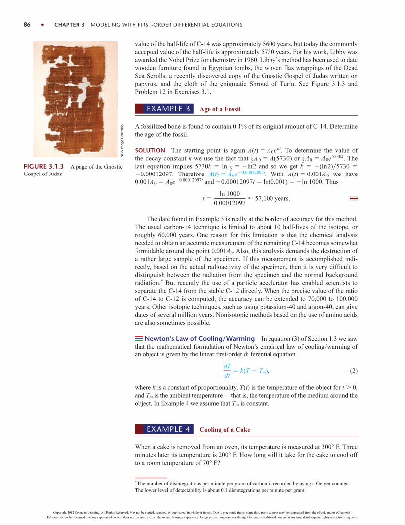
value of the half-life of C-14 was approximately 5600 years, but today the commonlyaccepted value of the half-life is approximately 5730 years. For his work, Libby wasawarded the Nobel Prize for chemistry in 1960. Libby’s method has been used to datewooden furniture found in Egyptian tombs, the woven flax wrappings of the DeadSea Scrolls, a recently discovered copy of the Gnostic Gospel of Judas written onpapyrus, and the cloth of the enigmatic Shroud of Turin. See Figure 3.1.3 andProblem 12 in Exercises 3.1.
86 CHAPTER 3 MODELING WITH FIRST-ORDER DIFFERENTIAL EQUATIONS
*The number of disintegrations per minute per gram of carbon is recorded by using a Geiger counter.The lower level of detectability is about 0.1 disintegrations per minute per gram.
EXAMPLE 3 Age of a Fossil
A fossilized bone is found to contain 0.1% of its original amount of C-14. Determinethe age of the fossil.
SOLUTION The starting point is again A(t) A0ekt. To determine the value ofthe decay constant k we use the fact that A0 A(5730) or A0 A0e5730k. Thelast equation implies 5730k ln ln2 and so we get k (ln2)5730 0.00012097. Therefore A(t) A0e0.00012097t. With A(t) 0.001A0 we have0.001A0 A0e0.00012097t and 0.00012097t ln(0.001) ln 1000. Thus
.
The date found in Example 3 is really at the border of accuracy for this method.The usual carbon-14 technique is limited to about 10 half-lives of the isotope, orroughly years. One reason for this limitation is that the chemical analysisneeded to obtain an accurate measurement of the remaining C-14 becomes somewhatformidable around the point Also, this analysis demands the destruction ofa rather large sample of the specimen. If this measurement is accomplished indi-rectly, based on the actual radioactivity of the specimen, then it is very difficult todistinguish between the radiation from the specimen and the normal backgroundradiation.* But recently the use of a particle accelerator has enabled scientists toseparate the C-14 from the stable C-12 directly. When the precise value of the ratioof C-14 to C-12 is computed, the accuracy can be extended to 70,000 to 100,000years. Other isotopic techniques, such as using potassium-40 and argon-40, can givedates of several million years. Nonisotopic methods based on the use of amino acidsare also sometimes possible.
Newton’s Law of Cooling/Warming In equation (3) of Section 1.3 we sawthat the mathematical formulation of Newton’s empirical law of cooling/warming ofan object is given by the linear first-order di ferential equation
, (2)
where k is a constant of proportionality, T(t) is the temperature of the object for t 0,and Tm is the ambient temperature—that is, the temperature of the medium around theobject. In Example 4 we assume that Tm is constant.
dT
dt k(T Tm)
0.001A0.
60,000
t ln 1000
0.00012097 57,100 years
12
12
12
EXAMPLE 4 Cooling of a Cake
When a cake is removed from an oven, its temperature is measured at 300° F. Threeminutes later its temperature is 200° F. How long will it take for the cake to cool offto a room temperature of 70° F?
FIGURE 3.1.3 A page of the GnosticGospel of Judas
NG
S Im
age
Col
lect
ion
Copyright 2012 Cengage Learning. All Rights Reserved. May not be copied, scanned, or duplicated, in whole or in part. Due to electronic rights, some third party content may be suppressed from the eBook and/or eChapter(s).
Editorial review has deemed that any suppressed content does not materially affect the overall learning experience. Cengage Learning reserves the right to remove additional content at any time if subsequent rights restrictions require it.

3.1 LINEAR MODELS 87
SOLUTION In (2) we make the identification Tm 70. We must then solve theinitial-value problem
(3)
and determine the value of k so that T(3) 200.Equation (3) is both linear and separable. If we separate variables,
,
yields ln T 70 kt c1, and so T 70 c2ekt. When t 0, T 300, so300 70 c2 gives c2 230; therefore T 70 230ekt. Finally, the measurementT(3) 200 leads to , or ln . Thus
. (4)
We note that (4) furnishes no finite solution to T(t) 70, since .Yet we intuitively expect the cake to reach room temperature after a reasonably longperiod of time. How long is “long”? Of course, we should not be disturbed by the factthat the model (3) does not quite live up to our physical intuition. Parts (a) and (b) ofFigure 3.1.4 clearly show that the cake will be approximately at room temperature inabout one-half hour.
The ambient temperature in (2) need not be a constant but could be a functionTm(t) of time t. See Problem 18 in Exercises 3.1.
Mixtures The mixing of two fluids sometimes gives rise to a linear first-ordedifferential equation. When we discussed the mixing of two brine solutions inSection 1.3, we assumed that the rate A(t) at which the amount of salt in the mixingtank changes was a net rate:
. (5)
In Example 5 we solve equation (8) of Section 1.3.
dA
dt (input rate of salt) (output rate of salt) Rin Rout
lim t : T (t) 70
T (t) 70 230e0.19018t
1323 0.19018k 1
3e3k 1323
dT
T 70 k dt
dT
dt k(T 70), T(0) 300
t
T
15 30
300
150 T = 70
(a)
T(t) t (min)
75 20.174 21.373 22.872 24.971 28.670.5 32.3
(b)
FIGURE 3.1.4 Temperature of coolingcake in Example 4
EXAMPLE 5 Mixture of Two Salt Solutions
Recall that the large tank considered in Section 1.3 held 300 gallons of a brinesolution. Salt was entering and leaving the tank; a brine solution was being pumpedinto the tank at the rate of 3 gal/min; it mixed with the solution there, and then themixture was pumped out at the rate of 3 gal/min. The concentration of the saltin the inflo , or solution entering, was 2 lb/gal, so salt was entering the tank at therate Rin (2 lb/gal) (3 gal/min) 6 lb/min and leaving the tank at the rate Rout (A300 lb/gal) (3 gal/min) A100 lb/min. From this data and (5) we get equa-tion (8) of Section 1.3. Let us pose the question: If 50 pounds of salt were dissolvedinitially in the 300 gallons, how much salt is in the tank after a long time?
SOLUTION To find the amount of salt A(t) in the tank at time t, we solve the initial-value problem
.
Note here that the side condition is the initial amount of salt A(0) 50 in the tankand not the initial amount of liquid in the tank. Now since the integrating factor of thelinear differential equation is et/100, we can write the equation as
.d
dt [et/100A] 6et/100
dA
dt
1
100A 6, A(0) 50
Copyright 2012 Cengage Learning. All Rights Reserved. May not be copied, scanned, or duplicated, in whole or in part. Due to electronic rights, some third party content may be suppressed from the eBook and/or eChapter(s).
Editorial review has deemed that any suppressed content does not materially affect the overall learning experience. Cengage Learning reserves the right to remove additional content at any time if subsequent rights restrictions require it.
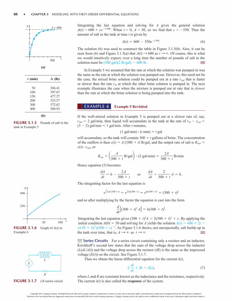
Integrating the last equation and solving for A gives the general solution A(t) 600 cet/100. When t 0, A 50, so we find that c 550. Thus theamount of salt in the tank at time t is given by
. (6)
The solution (6) was used to construct the table in Figure 3.1.5(b). Also, it can beseen from (6) and Figure 3.1.5(a) that A(t) : 600 as t : . Of course, this is whatwe would intuitively expect; over a long time the number of pounds of salt in thesolution must be (300 gal)(2 lb/gal) 600 lb.
In Example 5 we assumed that the rate at which the solution was pumped in wasthe same as the rate at which the solution was pumped out. However, this need not bethe case; the mixed brine solution could be pumped out at a rate rout that is fasteror slower than the rate rin at which the other brine solution is pumped in. The nextexample illustrates the case when the mixture is pumped out at rate that is slowerthan the rate at which the brine solution is being pumped into the tank.
A(t) 600 550et/100
88 CHAPTER 3 MODELING WITH FIRST-ORDER DIFFERENTIAL EQUATIONS
t
A A = 600
500
(a)
t (min) A (lb)
50 266.41100 397.67150 477.27200 525.57300 572.62400 589.93
(b)
FIGURE 3.1.5 Pounds of salt in thetank in Example 5
FIGURE 3.1.7 LR-series circuit
EL
R
FIGURE 3.1.6 Graph of A(t) inExample 6
t
A
50
250
500
100
EXAMPLE 6 Example 5 Revisited
If the well-stirred solution in Example 5 is pumped out at a slower rate of, say, rout 2 gal/min, then liquid will accumulate in the tank at the rate of rin rout (3 2) gal/min 1 gal/min. After t minutes,
(1 gal/min) . (t min) t gal
will accumulate, so the tank will contain 300 t gallons of brine. The concentrationof the outflow is then c(t) A(300 t) lb/gal, and the output rate of salt is Rout c(t) . rout, or
.
Hence equation (5) becomes
.
The integrating factor for the last equation is
and so after multiplying by the factor the equation is cast into the form
Integrating the last equation gives By applying theinitial condition and solving for A yields the solution A(t) 600 2t (4.95 107)(300 t)2. As Figure 3.1.6 shows, not unexpectedly, salt builds up inthe tank over time, that is,
Series Circuits For a series circuit containing only a resistor and an inductor,Kirchhoff’s second law states that the sum of the voltage drop across the inductor(L(didt)) and the voltage drop across the resistor (iR) is the same as the impressedvoltage (E(t)) on the circuit. See Figure 3.1.7.
Thus we obtain the linear differential equation for the current i(t),
, (7)
where L and R are constants known as the inductance and the resistance, respectively.The current i(t) is also called the response of the system.
Ldi
dt Ri E(t)
A : as t : .
A(0) 50(300 t)2A 2(300 t)3 c.
d
dt[(300 t)2 A] 6(300 t)2.
e2dt>(300 t) e2 ln(300 t) eln(300 t)2 (300 t)2
dA
dt 6
2A
300 tor
dA
dt
2
300 tA 6
Rout A
300 t lb/gal (2 gal/min)
2A
300 t lb/min
Copyright 2012 Cengage Learning. All Rights Reserved. May not be copied, scanned, or duplicated, in whole or in part. Due to electronic rights, some third party content may be suppressed from the eBook and/or eChapter(s).
Editorial review has deemed that any suppressed content does not materially affect the overall learning experience. Cengage Learning reserves the right to remove additional content at any time if subsequent rights restrictions require it.

3.1 LINEAR MODELS 89
R
C
E
FIGURE 3.1.8 RC-series circuit
The voltage drop across a capacitor with capacitance C is given by q(t)C,where q is the charge on the capacitor. Hence, for the series circuit shown inFigure 3.1.8, Kirchhoff’s second law gives
. (8)
But current i and charge q are related by i dqdt, so (8) becomes the linear differ-ential equation
. (9)Rdq
dt
1
Cq E(t)
Ri 1
Cq E(t)
FIGURE 3.1.9 Population growth is adiscrete process
t1t1 t2
P
P0
t1
P
P0
(a)
(b)
(c)
t1
P
P0
EXAMPLE 7 Series Circuit
A 12-volt battery is connected to a series circuit in which the inductance is henryand the resistance is 10 ohms. Determine the current i if the initial current is zero.
SOLUTION From (7) we see that we must solve
,
subject to i(0) 0. First, we multiply the differential equation by 2 and read off theintegrating factor e20t. We then obtain
.
Integrating each side of the last equation and solving for i gives i(t) ce20t.Now i(0) 0 implies that 0 c or c . Therefore the response is i(t) e20t.
From (4) of Section 2.3 we can write a general solution of (7):
. (10)
In particular, when E(t) E0 is a constant, (10) becomes
. (11)
Note that as t : , the second term in equation (11) approaches zero. Such a term is usu-ally called a transient term; any remaining terms are called the steady-state part of thesolution. In this case E0R is also called the steady-state current; for large values of timeit appears that the current in the circuit is simply governed by Ohm’s law (E iR).
i(t) E0
R ce(R/L)t
i(t) e(R/L)t
L e(R/L)tE(t) dt ce(R/L)t
65
65
65
65
65
d
dt [e20ti] 24e20t
1
2
di
dt 10 i 12
12
REMARKS
The solution P(t) P0e0.4055t of the initial-value problem in Example 1described the population of a colony of bacteria at any time t 0. Of course,P(t) is a continuous function that takes on all real numbers in the intervalP0 P . But since we are talking about a population, common sensedictates that P can take on only positive integer values. Moreover, we wouldnot expect the population to grow continuously—that is, every second, everymicrosecond, and so on—as predicted by our solution; there may be intervalsof time [t1, t2] over which there is no growth at all. Perhaps, then, the graphshown in Figure 3.1.9(a) is a more realistic description of P than is the graphof an exponential function. Using a continuous function to describe a discretephenomenon is often more a matter of convenience than of accuracy. However,for some purposes we may be satisfie if our model describes the systemfairly closely when viewed macroscopically in time, as in Figures 3.1.9(b)and 3.1.9(c), rather than microscopically, as in Figure 3.1.9(a).
Copyright 2012 Cengage Learning. All Rights Reserved. May not be copied, scanned, or duplicated, in whole or in part. Due to electronic rights, some third party content may be suppressed from the eBook and/or eChapter(s).
Editorial review has deemed that any suppressed content does not materially affect the overall learning experience. Cengage Learning reserves the right to remove additional content at any time if subsequent rights restrictions require it.
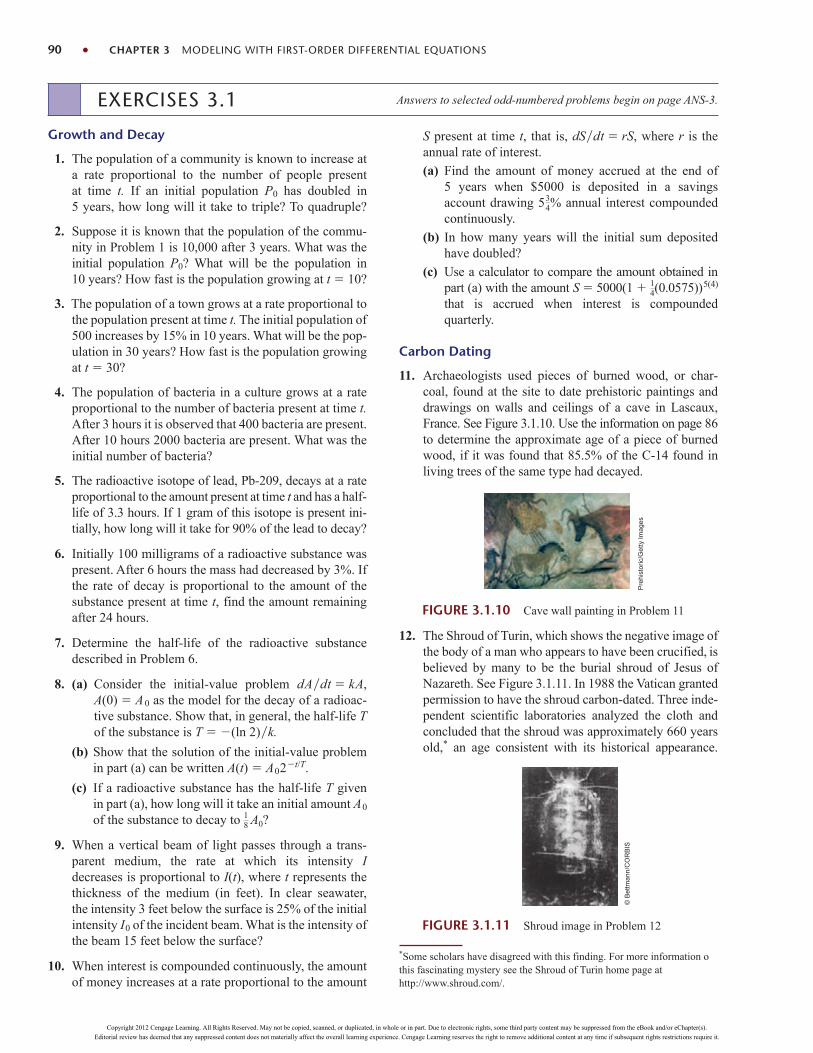
90 CHAPTER 3 MODELING WITH FIRST-ORDER DIFFERENTIAL EQUATIONS
EXERCISES 3.1 Answers to selected odd-numbered problems begin on page ANS-3.
Growth and Decay
1. The population of a community is known to increase ata rate proportional to the number of people presentat time t. If an initial population P0 has doubled in5 years, how long will it take to triple? To quadruple?
2. Suppose it is known that the population of the commu-nity in Problem 1 is 10,000 after 3 years. What was theinitial population P0? What will be the population in10 years? How fast is the population growing at t 10?
3. The population of a town grows at a rate proportional tothe population present at time t. The initial population of500 increases by 15% in 10 years. What will be the pop-ulation in 30 years? How fast is the population growingat t 30?
4. The population of bacteria in a culture grows at a rateproportional to the number of bacteria present at time t.After 3 hours it is observed that 400 bacteria are present.After 10 hours 2000 bacteria are present. What was theinitial number of bacteria?
5. The radioactive isotope of lead, Pb-209, decays at a rateproportional to the amount present at time t and has a half-life of 3.3 hours. If 1 gram of this isotope is present ini-tially, how long will it take for 90% of the lead to decay?
6. Initially 100 milligrams of a radioactive substance waspresent. After 6 hours the mass had decreased by 3%. Ifthe rate of decay is proportional to the amount of thesubstance present at time t, find the amount remainingafter 24 hours.
7. Determine the half-life of the radioactive substancedescribed in Problem 6.
8. (a) Consider the initial-value problem dAdt kA,A(0) A0 as the model for the decay of a radioac-tive substance. Show that, in general, the half-life Tof the substance is T (ln 2)k.
(b) Show that the solution of the initial-value problemin part (a) can be written A(t) A02t/T.
(c) If a radioactive substance has the half-life T givenin part (a), how long will it take an initial amount A0
of the substance to decay to ?
9. When a vertical beam of light passes through a trans-parent medium, the rate at which its intensity Idecreases is proportional to I(t), where t represents thethickness of the medium (in feet). In clear seawater,the intensity 3 feet below the surface is 25% of the initialintensity I0 of the incident beam. What is the intensity ofthe beam 15 feet below the surface?
10. When interest is compounded continuously, the amountof money increases at a rate proportional to the amount
18 A0
S present at time t, that is, dSdt rS, where r is theannual rate of interest.
(a) Find the amount of money accrued at the end of5 years when $5000 is deposited in a savingsaccount drawing 5 % annual interest compoundedcontinuously.
(b) In how many years will the initial sum depositedhave doubled?
(c) Use a calculator to compare the amount obtained inpart (a) with the amount S 5000(1 (0.0575))5(4)
that is accrued when interest is compoundedquarterly.
Carbon Dating
11. Archaeologists used pieces of burned wood, or char-coal, found at the site to date prehistoric paintings anddrawings on walls and ceilings of a cave in Lascaux,France. See Figure 3.1.10. Use the information on page 86to determine the approximate age of a piece of burnedwood, if it was found that 85.5% of the C-14 found inliving trees of the same type had decayed.
14
34
FIGURE 3.1.10 Cave wall painting in Problem 11
Pre
hist
oric
/Get
ty Im
ages
12. The Shroud of Turin, which shows the negative image ofthe body of a man who appears to have been crucified, isbelieved by many to be the burial shroud of Jesus ofNazareth. See Figure 3.1.11. In 1988 the Vatican grantedpermission to have the shroud carbon-dated. Three inde-pendent scientific laboratories analyzed the cloth andconcluded that the shroud was approximately 660 yearsold,* an age consistent with its historical appearance.
FIGURE 3.1.11 Shroud image in Problem 12
©B
ettm
ann
/CO
RB
IS
*Some scholars have disagreed with this finding. For more information othis fascinating mystery see the Shroud of Turin home page athttp://www.shroud.com/.
Copyright 2012 Cengage Learning. All Rights Reserved. May not be copied, scanned, or duplicated, in whole or in part. Due to electronic rights, some third party content may be suppressed from the eBook and/or eChapter(s).
Editorial review has deemed that any suppressed content does not materially affect the overall learning experience. Cengage Learning reserves the right to remove additional content at any time if subsequent rights restrictions require it.

3.1 LINEAR MODELS 91
Using this age, determine what percentage of the origi-nal amount of C-14 remained in the cloth as of 1988.
Newton’s Law of Cooling/Warming
13. A thermometer is removed from a room where thetemperature is 70° F and is taken outside, where the airtemperature is 10° F. After one-half minute the ther-mometer reads 50° F. What is the reading of the ther-mometer at t 1 min? How long will it take for thethermometer to reach 15° F?
14. A thermometer is taken from an inside room to the out-side, where the air temperature is 5° F. After 1 minutethe thermometer reads 55° F, and after 5 minutes itreads 30° F. What is the initial temperature of the insideroom?
15. A small metal bar, whose initial temperature was 20° C,is dropped into a large container of boiling water. Howlong will it take the bar to reach 90° C if it is known thatits temperature increases 2° in 1 second? How long will ittake the bar to reach 98° C?
16. Two large containers A and B of the same size are fillewith different fluids. The fluids in containers A and Bare maintained at 0° C and 100° C, respectively. A smallmetal bar, whose initial temperature is 100° C, is low-ered into container A. After 1 minute the temperatureof the bar is 90° C. After 2 minutes the bar is removedand instantly transferred to the other container. After1 minute in container B the temperature of the bar rises10°. How long, measured from the start of the entireprocess, will it take the bar to reach 99.9° C?
17. A thermometer reading 70° F is placed in an ovenpreheated to a constant temperature. Through a glasswindow in the oven door, an observer records that thethermometer reads 110° F after minute and 145° Fafter 1 minute. How hot is the oven?
18. At t 0 a sealed test tube containing a chemical isimmersed in a liquid bath. The initial temperature ofthe chemical in the test tube is 80° F. The liquid bathhas a controlled temperature (measured in degreesFahrenheit) given by Tm(t) 100 40e0.1t, t 0,where t is measured in minutes.
(a) Assume that k 0.1 in (2). Before solving theIVP, describe in words what you expect the temper-ature T(t) of the chemical to be like in the shortterm. In the long term.
(b) Solve the initial-value problem. Use a graphing util-ity to plot the graph of T(t) on time intervals of var-ious lengths. Do the graphs agree with yourpredictions in part (a)?
19. A dead body was found within a closed room of a housewhere the temperature was a constant 70° F. At the timeof discovery the core temperature of the body wasdetermined to be 85° F. One hour later a second mea-
12
surement showed that the core temperature of the bodywas 80° F. Assume that the time of death corresponds tot 0 and that the core temperature at that time was98.6° F. Determine how many hours elapsed before thebody was found. [Hint: Let t1 0 denote the time thatthe body was discovered.]
20. The rate at which a body cools also depends on itsexposed surface area S. If S is a constant, then a modification of (2) is
where k 0 and Tm is a constant. Suppose that two cupsA and B are filled with coffee at the same time. Initially,the temperature of the coffee is 150° F. The exposedsurface area of the coffee in cup B is twice the surfacearea of the coffee in cup A. After 30 min the temperatureof the coffee in cup A is 100° F. If Tm 70° F, then whatis the temperature of the coffee in cup B after 30 min?
Mixtures
21. A tank contains 200 liters of fluid in which 30 grams ofsalt is dissolved. Brine containing 1 gram of salt per literis then pumped into the tank at a rate of 4 L/min; thewell-mixed solution is pumped out at the same rate. Findthe number A(t) of grams of salt in the tank at time t.
22. Solve Problem 21 assuming that pure water is pumpedinto the tank.
23. A large tank is filled to capacity with 500 gallons of purewater. Brine containing 2 pounds of salt per gallon ispumped into the tank at a rate of 5 gal/min. The well-mixed solution is pumped out at the same rate. Find thenumber A(t) of pounds of salt in the tank at time t.
24. In Problem 23, what is the concentration c(t) of the saltin the tank at time t? At t 5 min? What is the concen-tration of the salt in the tank after a long time, that is, ast : ? At what time is the concentration of the salt inthe tank equal to one-half this limiting value?
25. Solve Problem 23 under the assumption that the solu-tion is pumped out at a faster rate of 10 gal/min. Whenis the tank empty?
26. Determine the amount of salt in the tank at time t inExample 5 if the concentration of salt in the inflow isvariable and given by cin(t) 2 sin(t4) lb/gal.Without actually graphing, conjecture what the solutioncurve of the IVP should look like. Then use a graphingutility to plot the graph of the solution on the interval[0, 300]. Repeat for the interval [0, 600] and compareyour graph with that in Figure 3.1.5(a).
27. A large tank is partially filled with 100 gallons of fluiin which 10 pounds of salt is dissolved. Brine containing
dT
dt kS(T Tm),
Copyright 2012 Cengage Learning. All Rights Reserved. May not be copied, scanned, or duplicated, in whole or in part. Due to electronic rights, some third party content may be suppressed from the eBook and/or eChapter(s).
Editorial review has deemed that any suppressed content does not materially affect the overall learning experience. Cengage Learning reserves the right to remove additional content at any time if subsequent rights restrictions require it.

pound of salt per gallon is pumped into the tank at arate of 6 gal/min. The well-mixed solution is thenpumped out at a slower rate of 4 gal/min. Find the num-ber of pounds of salt in the tank after 30 minutes.
28. In Example 5 the size of the tank containing the saltmixture was not given. Suppose, as in the discussionfollowing Example 5, that the rate at which brine ispumped into the tank is 3 gal/min but that the well-stirred solution is pumped out at a rate of 2 gal/min. Itstands to reason that since brine is accumulating in thetank at the rate of 1 gal/min, any finite tank must even-tually overflo . Now suppose that the tank has an opentop and has a total capacity of 400 gallons.
(a) When will the tank overflow
(b) What will be the number of pounds of salt in thetank at the instant it overflows
(c) Assume that although the tank is overflowing, brinesolution continues to be pumped in at a rate of3 gal/min and the well-stirred solution continues tobe pumped out at a rate of 2 gal/min. Devise amethod for determining the number of pounds ofsalt in the tank at t 150 minutes.
(d) Determine the number of pounds of salt in the tank ast : . Does your answer agree with your intuition?
(e) Use a graphing utility to plot the graph of A(t) onthe interval [0, 500).
Series Circuits
29. A 30-volt electromotive force is applied to an LR-seriescircuit in which the inductance is 0.1 henry and theresistance is 50 ohms. Find the current i(t) if i(0) 0.Determine the current as t : .
30. Solve equation (7) under the assumption that E(t) E0 sin vt and i(0) i0.
31. A 100-volt electromotive force is applied to an RC-series circuit in which the resistance is 200 ohms andthe capacitance is 104 farad. Find the charge q(t) onthe capacitor if q(0) 0. Find the current i(t).
32. A 200-volt electromotive force is applied to an RC-seriescircuit in which the resistance is 1000 ohms and thecapacitance is 5 106 farad. Find the charge q(t) on thecapacitor if i(0) 0.4. Determine the charge and currentat t 0.005 s. Determine the charge as t : .
33. An electromotive force
is applied to an LR-series circuit in which the inductanceis 20 henries and the resistance is 2 ohms. Find thecurrent i(t) if i(0) 0.
E(t) 120,
0,
0 t 20
t 20
12
92 CHAPTER 3 MODELING WITH FIRST-ORDER DIFFERENTIAL EQUATIONS
34. Suppose an RC-series circuit has a variable resistor. If theresistance at time t is given by R k1 k2t, where k1 andk2 are known positive constants, then (9) becomes
.
If E(t) E0 and q(0) q0, where E0 and q0 areconstants, show that
.
Additional Linear Models
35. Air Resistance In (14) of Section 1.3 we saw thata differential equation describing the velocity v of afalling mass subject to air resistance proportional to theinstantaneous velocity is
,
where k 0 is a constant of proportionality. The positivedirection is downward.
(a) Solve the equation subject to the initial conditionv(0) v0.
(b) Use the solution in part (a) to determine the limit-ing, or terminal, velocity of the mass. We saw howto determine the terminal velocity without solvingthe DE in Problem 40 in Exercises 2.1.
(c) If the distance s, measured from the point where themass was released above ground, is related to ve-locity v by dsdt v(t), find an explicit expressionfor s(t) if s(0) 0.
36. How High?—No Air Resistance Suppose a smallcannonball weighing 16 pounds is shot verticallyupward, as shown in Figure 3.1.12, with an initial veloc-ity v0 300 ft/s. The answer to the question “How highdoes the cannonball go?” depends on whether we takeair resistance into account.
(a) Suppose air resistance is ignored. If the positivedirection is upward, then a model for the state ofthe cannonball is given by d2sdt2 g (equation(12) of Section 1.3). Since dsdt v(t) the last
mdv
dt mg kv
q(t) E0C (q0 E0C ) k1
k1 k2t
1/Ck2
(k1 k2t)dq
dt
1
Cq E(t)
FIGURE 3.1.12 Find themaximum height of the cannonballin Problem 36
groundlevel
−mg
Copyright 2012 Cengage Learning. All Rights Reserved. May not be copied, scanned, or duplicated, in whole or in part. Due to electronic rights, some third party content may be suppressed from the eBook and/or eChapter(s).
Editorial review has deemed that any suppressed content does not materially affect the overall learning experience. Cengage Learning reserves the right to remove additional content at any time if subsequent rights restrictions require it.

3.1 LINEAR MODELS 93
differential equation is the same as dvdt g,where we take g 32 ft /s2. Find the velocity v(t)of the cannonball at time t.
(b) Use the result obtained in part (a) to determine theheight s(t) of the cannonball measured from groundlevel. Find the maximum height attained by thecannonball.
37. How High?—Linear Air Resistance Repeat Prob-lem 36, but this time assume that air resistance isproportional to instantaneous velocity. It stands toreason that the maximum height attained by the cannon-ball must be less than that in part (b) of Problem 36.Show this by supposing that the constant of proportion-ality is k 0.0025. [Hint: Slightly modify the DE inProblem 35.]
38. Skydiving A skydiver weighs 125 pounds, and herparachute and equipment combined weigh another 35pounds. After exiting from a plane at an altitude of15,000 feet, she waits 15 seconds and opens her para-chute. Assume that the constant of proportionality inthe model in Problem 35 has the value k 0.5 duringfree fall and k 10 after the parachute is opened.Assume that her initial velocity on leaving the plane iszero. What is her velocity and how far has she traveled20 seconds after leaving the plane? See Figure 3.1.13.How does her velocity at 20 seconds compare with herterminal velocity? How long does it take her to reach theground? [Hint: Think in terms of two distinct IVPs.]
and the downward direction is taken to be the positivedirection.
(a) Solve for v(t) if the raindrop falls from rest.
(b) Reread Problem 36 of Exercises 1.3 and thenshow that the radius of the raindrop at time t isr(t) (kr)t r0.
(c) If r0 0.01 ft and r 0.007 ft 10 seconds after theraindrop falls from a cloud, determine the time atwhich the raindrop has evaporated completely.
40. Fluctuating Population The differential equationdPdt (k cos t)P, where k is a positive constant, is amathematical model for a population P(t) that under-goes yearly seasonal fluctuations. Solve the equationsubject to P(0) P0. Use a graphing utility to graph thesolution for different choices of P0.
41. Population Model In one model of the changingpopulation P(t) of a community, it is assumed that
,
where dBdt and dDdt are the birth and death rates,respectively.
(a) Solve for P(t) if dBdt k1P and dDdt k2P.
(b) Analyze the cases k1 k2, k1 k2, and k1 k2.
42. Constant-Harvest Model A model that describes thepopulation of a fishery in which harvesting takes place ata constant rate is given by
where k and h are positive constants.
(a) Solve the DE subject to P(0) P0.
(b) Describe the behavior of the population P(t) for in-creasing time in the three cases P0 hk, P0 hk,and 0 P0 hk.
(c) Use the results from part (b) to determine whetherthe fish population will ever go extinct in finittime, that is, whether there exists a time T 0such that P(T) 0. If the population goes extinct,then find T.
43. Drug Dissemination A mathematical model for therate at which a drug disseminates into the bloodstreamis given by
where r and k are positive constants. The function x(t)describes the concentration of the drug in the blood-stream at time t.
(a) Since the DE is autonomous, use the phase portraitconcept of Section 2.1 to find the limiting value ofx(t) as t : .
dx
dt r kx,
dP
dt kP h,
dP
dt
dB
dt
dD
dt
FIGURE 3.1.13Find the time toreach the ground inProblem 38
free fall
parachute opens
air resistance is 0.5v
air resistance is 10v
t = 20 s
39. Evaporating Raindrop As a raindrop falls, it evapo-rates while retaining its spherical shape. If we make thefurther assumptions that the rate at which the raindropevaporates is proportional to its surface area and that airresistance is negligible, then a model for the velocityv(t) of the raindrop is
.
Here r is the density of water, r0 is the radius of the rain-drop at t 0, k 0 is the constant of proportionality,
dv
dt
3(k/)
(k/)t r0 v g
Copyright 2012 Cengage Learning. All Rights Reserved. May not be copied, scanned, or duplicated, in whole or in part. Due to electronic rights, some third party content may be suppressed from the eBook and/or eChapter(s).
Editorial review has deemed that any suppressed content does not materially affect the overall learning experience. Cengage Learning reserves the right to remove additional content at any time if subsequent rights restrictions require it.

(b) Solve the DE subject to x(0) 0. Sketch the graphof x(t) and verify your prediction in part (a). Atwhat time is the concentration one-half this limitingvalue?
44. Memorization When forgetfulness is taken intoaccount, the rate of memorization of a subject is given by
,
where k1 0, k2 0, A(t) is the amount memorizedin time t, M is the total amount to be memorized, andM A is the amount remaining to be memorized.
(a) Since the DE is autonomous, use the phase portraitconcept of Section 2.1 to find the limiting value ofA(t) as t : . Interpret the result.
(b) Solve the DE subject to A(0) 0. Sketch the graphof A(t) and verify your prediction in part (a).
45. Heart Pacemaker A heart pacemaker, shown inFigure 3.1.14, consists of a switch, a battery, a capacitor,and the heart as a resistor. When the switch S is at P, thecapacitor charges; when S is at Q, the capacitor dis-charges, sending an electrical stimulus to the heart. InProblem 53 in Exercises 2.3 we saw that during thistime the electrical stimulus is being applied to the heart,the voltage E across the heart satisfies the linear D
.
(a) Let us assume that over the time interval of lengtht1, 0 t t1, the switch S is at position P shownin Figure 3.1.14 and the capacitor is beingcharged. When the switch is moved to positionQ at time t1 the capacitor discharges, sending animpulse to the heart over the time interval oflength t2: t1 t t1 t2. Thus over the initialcharging/discharging interval 0 t t1 t2 thevoltage to the heart is actually modeled by thepiecewise-defined differential equation
.
dE
dt 0,
1
RCE,
0 t t1
t1 t t1 t2
dE
dt
1
RC E
dA
dt k1(M A) k2A
94 CHAPTER 3 MODELING WITH FIRST-ORDER DIFFERENTIAL EQUATIONS
By moving S between P and Q, the charging anddischarging over time intervals of lengths t1 and t2
is repeated indefinitel . Suppose t1 4 s, t2 2 s,E0 12 V, and E(0) 0, E(4) 12, E(6) 0,E(10) 12, E(12) 0, and so on. Solve for E(t)for 0 t 24.
(b) Suppose for the sake of illustration that R C 1.Use a graphing utility to graph the solution for theIVP in part (a) for 0 t 24.
46. Sliding Box (a) A box of mass m slides down aninclined plane that makes an angle u with the hori-zontal as shown in Figure 3.1.15. Find a differentialequation for the velocity v(t) of the box at time t ineach of the following three cases:
(i) No sliding friction and no air resistance(ii) With sliding friction and no air resistance(iii) With sliding friction and air resistance
In cases (ii) and (iii), use the fact that the force offriction opposing the motion of the box is mN,where m is the coefficient of sliding friction and Nis the normal component of the weight of the box.In case (iii) assume that air resistance is propor-tional to the instantaneous velocity.
(b) In part (a), suppose that the box weighs 96 pounds,that the angle of inclination of the plane is u 30°,that the coefficient of sliding friction is ,and that the additional retarding force due to airresistance is numerically equal to v. Solve the dif-ferential equation in each of the three cases, assum-ing that the box starts from rest from the highestpoint 50 ft above ground.
14
134
heart
C
Q
P Sswitch
E0
R
FIGURE 3.1.14 Model of a pacemaker in Problem 45
FIGURE 3.1.15 Box sliding down inclined plane inProblem 46
θ
50 ftmotion
friction
W = mg
47. Sliding Box—Continued (a) In Problem 46 let s(t) bethe distance measured down the inclined planefrom the highest point. Use dsdt v(t) and thesolution for each of the three cases in part (b) ofProblem 46 to find the time that it takes the box toslide completely down the inclined plane. A root-finding application of a CAS may be useful here.
(b) In the case in which there is friction (m 0) but noair resistance, explain why the box will not slidedown the plane starting from rest from the highest
Copyright 2012 Cengage Learning. All Rights Reserved. May not be copied, scanned, or duplicated, in whole or in part. Due to electronic rights, some third party content may be suppressed from the eBook and/or eChapter(s).
Editorial review has deemed that any suppressed content does not materially affect the overall learning experience. Cengage Learning reserves the right to remove additional content at any time if subsequent rights restrictions require it.

point above ground when the inclination angle usatisfies tan u m.
(c) The box will slide downward on the plane whentan u m if it is given an initial velocity v(0) v0 0. Suppose that and u 23°. Verify that tan u m. How far will thebox slide down the plane if v0 1 ft /s?
(d) Using the values and u 23°, approxi-mate the smallest initial velocity v0 that can be givento the box so that, starting at the highest point 50 ftabove ground, it will slide completely down the in-clined plane. Then find the corresponding time ittakes to slide down the plane.
134
134
3.2 NONLINEAR MODELS 95
48. What Goes Up . . . (a) It is well known that themodel in which air resistance is ignored, part (a) ofProblem 36, predicts that the time ta it takes thecannonball to attain its maximum height is thesame as the time td it takes the cannonball to fallfrom the maximum height to the ground. Moreover,the magnitude of the impact velocity vi will be thesame as the initial velocity v0 of the cannonball.Verify both of these results.
(b) Then, using the model in Problem 37 that takes airresistance into account, compare the value of ta
with td and the value of the magnitude of vi with v0.A root-finding application of a CAS (or graphic cal-culator) may be useful here.
NONLINEAR MODELS
REVIEW MATERIAL Equations (5), (6), and (10) of Section 1.3 and Problems 7, 8, 13, 14, and 17 of Exercises 1.3 Separation of variables in Section 2.2
INTRODUCTION We finish our study of single first-order differential equations with an exam-ination of some nonlinear models.
3.2
Population Dynamics If P(t) denotes the size of a population at time t, the
P
f (P)
r
K
FIGURE 3.2.1 Simplest assumptionfor f (P) is a straight line (blue color)
model for exponential growth begins with the assumption that dPdt kP for somek 0. In this model, the relative, or specific, g owth rate defined b
(1)
is a constant k. True cases of exponential growth over long periods of time are hardto find because the limited resources of the environment will at some time exertrestrictions on the growth of a population. Thus for other models, (1) can be expectedto decrease as the population P increases in size.
The assumption that the rate at which a population grows (or decreases) isdependent only on the number P present and not on any time-dependent mechanismssuch as seasonal phenomena (see Problem 33 in Exercises 1.3) can be stated as
. (2)
The differential equation in (2), which is widely assumed in models of animalpopulations, is called the density-dependent hypothesis.
Logistic Equation Suppose an environment is capable of sustaining no morethan a fixed number K of individuals in its population. The quantity K is called thecarrying capacity of the environment. Hence for the function f in (2) we havef (K ) 0, and we simply let f (0) r. Figure 3.2.1 shows three functions f that sat-isfy these two conditions. The simplest assumption that we can make is that f (P)is linear—that is, f (P) c1P c2. If we use the conditions f (0) r and f (K ) 0,
dP>dt
P f (P) or
dP
dt Pf (P)
dP>dt
P
Copyright 2012 Cengage Learning. All Rights Reserved. May not be copied, scanned, or duplicated, in whole or in part. Due to electronic rights, some third party content may be suppressed from the eBook and/or eChapter(s).
Editorial review has deemed that any suppressed content does not materially affect the overall learning experience. Cengage Learning reserves the right to remove additional content at any time if subsequent rights restrictions require it.

96 CHAPTER 3 MODELING WITH FIRST-ORDER DIFFERENTIAL EQUATIONS
we find, in turn, c2 r and c1 rK, and so f takes on the form f (P) r (rK)P.Equation (2) becomes
. (3)
With constants relabeled, the nonlinear equation (3) is the same as
. (4)
Around 1840 the Belgian mathematician-biologist P. F. Verhulst (1804–1849)was concerned with mathematical models for predicting the human populations ofvarious countries. One of the equations he studied was (4), where a 0 and b 0.Equation (4) came to be known as the logistic equation, and its solution is called thelogistic function. The graph of a logistic function is called a logistic curve.
The linear differential equation dPdt kP does not provide a very accuratemodel for population when the population itself is very large. Overcrowded condi-tions, with the resulting detrimental effects on the environment such as pollution andexcessive and competitive demands for food and fuel, can have an inhibiting effecton population growth. As we shall now see, the solution of (4) is bounded as t : .If we rewrite (4) as dPdt aP bP2, the nonlinear term bP2, b 0, can be in-terpreted as an “inhibition” or “competition” term. Also, in most applications thepositive constant a is much larger than the constant b.
Logistic curves have proved to be quite accurate in predicting the growthpatterns, in a limited space, of certain types of bacteria, protozoa, water flea(Daphnia), and fruit flies Drosophila).
Solution of the Logistic Equation One method of solving (4) is separation
dP
dt P(a bP)
dP
dt Pr
r
KP
of variables. Decomposing the left side of dPP(a bP) dt into partial fractionsand integrating gives
It follows from the last equation that
.
If P(0) P0, P0 ab, we find c1 P0(a bP0), and so after substituting andsimplifying, the solution becomes
. (5)
Graphs of P(t) The basic shape of the graph of the logistic function P(t) can beobtained without too much effort. Although the variable t usually represents time andwe are seldom concerned with applications in which t 0, it is nonetheless of some in-terest to include this interval in displaying the various graphs of P. From (5) we see that
.P(t) :aP0
bP0
a
bas t : and P(t) : 0 as t :
P(t) aP0
bP0 (a bP0)eat
P(t) ac1eat
1 bc1eat ac1
bc1 eat
P
a bP c1eat.
ln P
a bP at ac
1
a ln P
1
a ln a bP t c
1>aP
b>a
a bPdP dt
Copyright 2012 Cengage Learning. All Rights Reserved. May not be copied, scanned, or duplicated, in whole or in part. Due to electronic rights, some third party content may be suppressed from the eBook and/or eChapter(s).
Editorial review has deemed that any suppressed content does not materially affect the overall learning experience. Cengage Learning reserves the right to remove additional content at any time if subsequent rights restrictions require it.
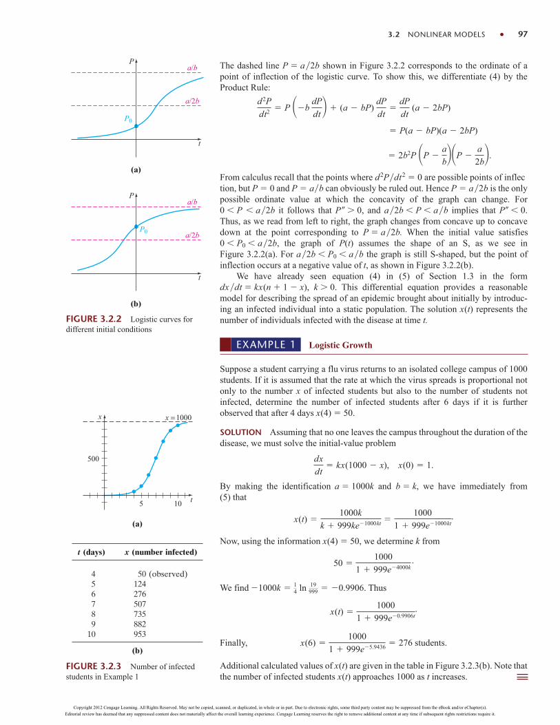
The dashed line P a2b shown in Figure 3.2.2 corresponds to the ordinate of apoint of inflection of the logistic curve. To show this, we differentiate (4) by theProduct Rule:
.
From calculus recall that the points where d2Pdt2 0 are possible points of inflection, but P 0 and P ab can obviously be ruled out. Hence P a2b is the onlypossible ordinate value at which the concavity of the graph can change. For 0 P a2b it follows that P 0, and a2b P ab implies that P 0.Thus, as we read from left to right, the graph changes from concave up to concavedown at the point corresponding to P a2b. When the initial value satisfies0 P0 a2b, the graph of P(t) assumes the shape of an S, as we see inFigure 3.2.2(a). For a2b P0 ab the graph is still S-shaped, but the point ofinflection occurs at a negative value of t, as shown in Figure 3.2.2(b).
We have already seen equation (4) in (5) of Section 1.3 in the form dxdt kx(n 1 x), k 0. This differential equation provides a reasonablemodel for describing the spread of an epidemic brought about initially by introduc-ing an infected individual into a static population. The solution x(t) represents thenumber of individuals infected with the disease at time t.
2b2P P a
bP a
2b P(a bP)(a 2bP)
d 2P
dt2 P bdP
dt (a bP) dP
dt
dP
dt (a 2bP)
3.2 NONLINEAR MODELS 97
P
P0
a/2b
a/b
t
P
P0 a/2b
a/b
t
(a)(a)
(b)
FIGURE 3.2.2 Logistic curves fordifferent initial conditions
(a)
t
x x = 1000
10
500
5
(a)
t (days) x (number infected)
4 50 (observed)5 1246 2767 5078 7359 882
10 953
(b)
FIGURE 3.2.3 Number of infectedstudents in Example 1
EXAMPLE 1 Logistic Growth
Suppose a student carrying a flu virus returns to an isolated college campus of 1000students. If it is assumed that the rate at which the virus spreads is proportional notonly to the number x of infected students but also to the number of students notinfected, determine the number of infected students after 6 days if it is furtherobserved that after 4 days x(4) 50.
SOLUTION Assuming that no one leaves the campus throughout the duration of thedisease, we must solve the initial-value problem
.
By making the identification a 1000k and b k, we have immediately from(5) that
.
Now, using the information x(4) 50, we determine k from
We find . Thus
.
Finally, .
Additional calculated values of x(t) are given in the table in Figure 3.2.3(b). Note thatthe number of infected students x(t) approaches 1000 as t increases.
x(6) 1000
1 999e5.9436 276 students
x(t) 1000
1 999e0.9906t
1000k 14 ln 19
999 0.9906
50 1000
1 999e4000k.
x(t) 1000k
k 999ke1000kt 1000
1 999e1000kt
dx
dt kx(1000 x), x(0) 1
Copyright 2012 Cengage Learning. All Rights Reserved. May not be copied, scanned, or duplicated, in whole or in part. Due to electronic rights, some third party content may be suppressed from the eBook and/or eChapter(s).
Editorial review has deemed that any suppressed content does not materially affect the overall learning experience. Cengage Learning reserves the right to remove additional content at any time if subsequent rights restrictions require it.
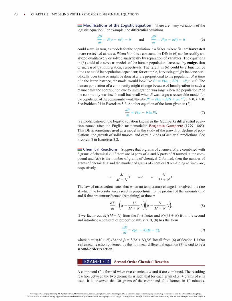
Modifications of the Logistic Equation There are many variations of thelogistic equation. For example, the differential equations
and (6)
could serve, in turn, as models for the population in a fisher where fis are harvestedor are restocked at rate h. When h 0 is a constant, the DEs in (6) can be readily an-alyzed qualitatively or solved analytically by separation of variables. The equationsin (6) could also serve as models of the human population decreased by emigrationor increased by immigration, respectively. The rate h in (6) could be a function oftime t or could be population dependent; for example, harvesting might be done peri-odically over time or might be done at a rate proportional to the population P at timet. In the latter instance, the model would look like P P(a bP) cP, c 0. Thehuman population of a community might change because of immigration in such amanner that the contribution due to immigration was large when the population P ofthe community was itself small but small when P was large; a reasonable model forthe population of the community would then be P P(a bP) cekP, c 0, k 0.See Problem 24 in Exercises 3.2. Another equation of the form given in (2),
, (7)
is a modification of the logistic equation known as the Gompertz differential equa-tion named after the English mathematician Benjamin Gompertz (1779–1865).This DE is sometimes used as a model in the study of the growth or decline of pop-ulations, the growth of solid tumors, and certain kinds of actuarial predictions. SeeProblem 8 in Exercises 3.2.
Chemical Reactions Suppose that a grams of chemical A are combined withb grams of chemical B. If there are M parts of A and N parts of B formed in the com-pound and X(t) is the number of grams of chemical C formed, then the number ofgrams of chemical A and the number of grams of chemical B remaining at time t are,respectively,
.
The law of mass action states that when no temperature change is involved, the rateat which the two substances react is proportional to the product of the amounts of Aand B that are untransformed (remaining) at time t:
. (8)
If we factor out M(M N) from the first factor and N(M N) from the secondand introduce a constant of proportionality k 0, (8) has the form
, (9)
where a a(M N)M and b b(M N)N. Recall from (6) of Section 1.3 thata chemical reaction governed by the nonlinear differential equation (9) is said to be asecond-order reaction.
dX
dt k( X)( X)
dX
dt a
M
M NXb
N
M NX
a M
M NX and b
N
M NX
dP
dt P(a b ln P)
dP
dt P(a bP) h
dP
dt P(a bP) h
98 CHAPTER 3 MODELING WITH FIRST-ORDER DIFFERENTIAL EQUATIONS
EXAMPLE 2 Second-Order Chemical Reaction
A compound C is formed when two chemicals A and B are combined. The resultingreaction between the two chemicals is such that for each gram of A, 4 grams of B isused. It is observed that 30 grams of the compound C is formed in 10 minutes.
Copyright 2012 Cengage Learning. All Rights Reserved. May not be copied, scanned, or duplicated, in whole or in part. Due to electronic rights, some third party content may be suppressed from the eBook and/or eChapter(s).
Editorial review has deemed that any suppressed content does not materially affect the overall learning experience. Cengage Learning reserves the right to remove additional content at any time if subsequent rights restrictions require it.

Determine the amount of C at time t if the rate of the reaction is proportional to theamounts of A and B remaining and if initially there are 50 grams of A and 32 gramsof B. How much of the compound C is present at 15 minutes? Interpret the solutionas t : .
SOLUTION Let X(t) denote the number of grams of the compound C present attime t. Clearly, X(0) 0 g and X(10) 30 g.
If, for example, 2 grams of compound C is present, we must have used,say, a grams of A and b grams of B, so a b 2 and b 4a. Thus we must usea 2 g of chemical A and b 2 g of B. In general, for X grams ofC we must use
.
The amounts of A and B remaining at time t are then
,
respectively.Now we know that the rate at which compound C is formed satisfie
.
To simplify the subsequent algebra, we factor from the first term and from thesecond and then introduce the constant of proportionality:
.
By separation of variables and partial fractions we can write
.
Integrating gives
(10)
When t 0, X 0, so it follows at this point that c2 . Using X 30 g at t 10,we find 210k ln 0.1258. With this information we solve the last equationin (10) for X:
. (11)
From (11) we find X(15) 34.78 grams. The behavior of X as a function of time is displayed in Figure 3.2.4. It is clear from the accompanying table and (11) that X : 40 as t : . This means that 40 grams of compound C is formed, leaving
.50 1
5(40) 42 g of A and 32
4
5(40) 0 g of B
X(t) 10001 e0.1258t
25 4e0.1258t
8825
110
254
ln 250 X
40 X 210kt c1 or
250 X
40 X c2e210kt.
1210
250 X dX
1210
40 X dX k dt
dX
dt k(250 X )(40 X )
45
15
dX
dt 50
1
5 X32
4
5X
50 1
5 X and 32
4
5 X
1
5 X grams of A and
4
5 X grams of B
(45)8
5(15)2
5
3.2 NONLINEAR MODELS 99
10 20 30 40 t
XX = 40
(a)
t (min) X (g)
10 30 (measured)15 34.7820 37.2525 38.5430 39.2235 39.59
(b)
FIGURE 3.2.4 Number of grams ofcompound C in Example 2
Copyright 2012 Cengage Learning. All Rights Reserved. May not be copied, scanned, or duplicated, in whole or in part. Due to electronic rights, some third party content may be suppressed from the eBook and/or eChapter(s).
Editorial review has deemed that any suppressed content does not materially affect the overall learning experience. Cengage Learning reserves the right to remove additional content at any time if subsequent rights restrictions require it.

100 CHAPTER 3 MODELING WITH FIRST-ORDER DIFFERENTIAL EQUATIONS
REMARKS
The indefinite integral du(a2 u2) can be evaluated in terms of logarithms,the inverse hyperbolic tangent, or the inverse hyperbolic cotangent. For example,of the two results
(12)
(13)
(12) may be convenient in Problems 15 and 26 in Exercises 3.2, whereas (13)may be preferable in Problem 27.
du
a 2 u 2 1
2a ln a u
a u c, u a,
du
a 2 u 2 1
atanh1
u
a c, u a
EXERCISES 3.2 Answers to selected odd-numbered problems begin on page ANS-3.
Logistic Equation
1. The number N(t) of supermarkets throughout the countrythat are using a computerized checkout system isdescribed by the initial-value problem
.
(a) Use the phase portrait concept of Section 2.1 to pre-dict how many supermarkets are expected to adoptthe new procedure over a long period of time. Byhand, sketch a solution curve of the given initial-value problem.
(b) Solve the initial-value problem and then use a graph-ing utility to verify the solution curve in part (a).How many companies are expected to adopt the newtechnology when t 10?
2. The number N(t) of people in a community who areexposed to a particular advertisement is governed bythe logistic equation. Initially, N(0) 500, and it isobserved that N(1) 1000. Solve for N(t) if it is pre-dicted that the limiting number of people in the commu-nity who will see the advertisement is 50,000.
3. A model for the population P(t) in a suburb of a largecity is given by the initial-value problem
,
where t is measured in months. What is the limitingvalue of the population? At what time will the popula-tion be equal to one-half of this limiting value?
4. (a) Census data for the United States between 1790 and1950 are given in Table 3.2.1. Construct a logisticpopulation model using the data from 1790, 1850,and 1910.
dP
dt P(101 107 P), P(0) 5000
dN
dt N(1 0.0005N ), N(0) 1
(b) Construct a table comparing actual census popula-tion with the population predicted by the model inpart (a). Compute the error and the percentage errorfor each entry pair.
Modifications of the Logistic Model
5. (a) If a constant number h of fish are harvested from afishery per unit time, then a model for the popula-tion P(t) of the fishery at time t is given by
,
where a, b, h, and P0 are positive constants.Suppose a 5, b 1, and h 4. Since the DE isautonomous, use the phase portrait concept ofSection 2.1 to sketch representative solution curves
dP
dt P(a bP) h, P(0) P0
TABLE 3.2.1
Year Population (in millions)
1790 3.9291800 5.3081810 7.2401820 9.6381830 12.8661840 17.0691850 23.1921860 31.4331870 38.5581880 50.1561890 62.9481900 75.9961910 91.9721920 105.7111930 122.7751940 131.6691950 150.697
Copyright 2012 Cengage Learning. All Rights Reserved. May not be copied, scanned, or duplicated, in whole or in part. Due to electronic rights, some third party content may be suppressed from the eBook and/or eChapter(s).
Editorial review has deemed that any suppressed content does not materially affect the overall learning experience. Cengage Learning reserves the right to remove additional content at any time if subsequent rights restrictions require it.
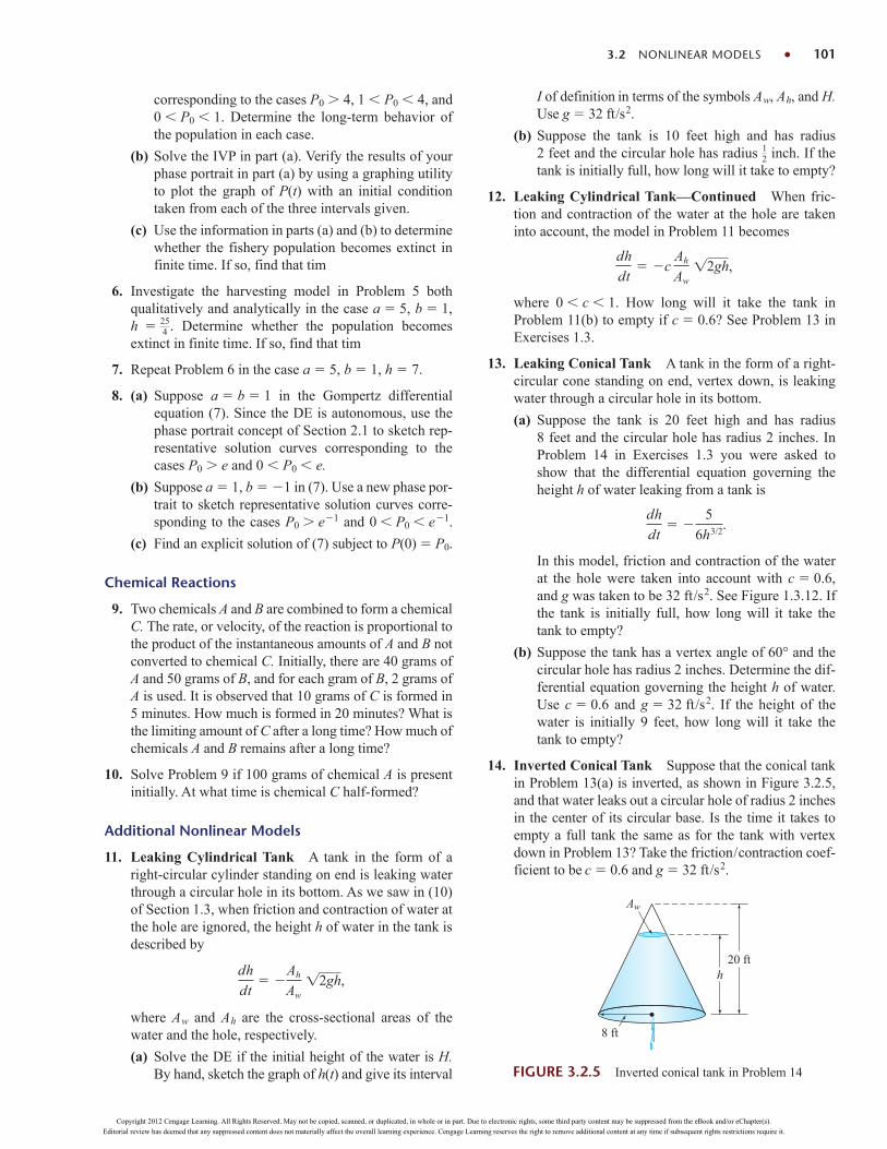
3.2 NONLINEAR MODELS 101
corresponding to the cases P0 4, 1 P0 4, and0 P0 1. Determine the long-term behavior ofthe population in each case.
(b) Solve the IVP in part (a). Verify the results of yourphase portrait in part (a) by using a graphing utilityto plot the graph of P(t) with an initial conditiontaken from each of the three intervals given.
(c) Use the information in parts (a) and (b) to determinewhether the fishery population becomes extinct infinite time. If so, find that tim
6. Investigate the harvesting model in Problem 5 bothqualitatively and analytically in the case a 5, b 1,h . Determine whether the population becomesextinct in finite time. If so, find that tim
7. Repeat Problem 6 in the case a 5, b 1, h 7.
8. (a) Suppose a b 1 in the Gompertz differentialequation (7). Since the DE is autonomous, use thephase portrait concept of Section 2.1 to sketch rep-resentative solution curves corresponding to thecases P0 e and 0 P0 e.
(b) Suppose a 1, b 1 in (7). Use a new phase por-trait to sketch representative solution curves corre-sponding to the cases P0 e1 and 0 P0 e1.
(c) Find an explicit solution of (7) subject to P(0) P0.
Chemical Reactions
9. Two chemicals A and B are combined to form a chemicalC. The rate, or velocity, of the reaction is proportional tothe product of the instantaneous amounts of A and B notconverted to chemical C. Initially, there are 40 grams ofA and 50 grams of B, and for each gram of B, 2 grams ofA is used. It is observed that 10 grams of C is formed in5 minutes. How much is formed in 20 minutes? What isthe limiting amount of C after a long time? How much ofchemicals A and B remains after a long time?
10. Solve Problem 9 if 100 grams of chemical A is presentinitially. At what time is chemical C half-formed?
Additional Nonlinear Models
11. Leaking Cylindrical Tank A tank in the form of aright-circular cylinder standing on end is leaking waterthrough a circular hole in its bottom. As we saw in (10)of Section 1.3, when friction and contraction of water atthe hole are ignored, the height h of water in the tank isdescribed by
,
where Aw and Ah are the cross-sectional areas of thewater and the hole, respectively.
(a) Solve the DE if the initial height of the water is H.By hand, sketch the graph of h(t) and give its interval
dh
dt
Ah
Aw
12gh
254
I of definition in terms of the symbols Aw, Ah, and H.Use g 32 ft/s2.
(b) Suppose the tank is 10 feet high and has radius2 feet and the circular hole has radius inch. If thetank is initially full, how long will it take to empty?
12. Leaking Cylindrical Tank—Continued When fric-tion and contraction of the water at the hole are takeninto account, the model in Problem 11 becomes
,
where 0 c 1. How long will it take the tank inProblem 11(b) to empty if c 0.6? See Problem 13 inExercises 1.3.
13. Leaking Conical Tank A tank in the form of a right-circular cone standing on end, vertex down, is leakingwater through a circular hole in its bottom.
(a) Suppose the tank is 20 feet high and has radius8 feet and the circular hole has radius 2 inches. InProblem 14 in Exercises 1.3 you were asked toshow that the differential equation governing theheight h of water leaking from a tank is
.
In this model, friction and contraction of the waterat the hole were taken into account with c 0.6,and g was taken to be 32 ft/s2. See Figure 1.3.12. Ifthe tank is initially full, how long will it take thetank to empty?
(b) Suppose the tank has a vertex angle of 60° and thecircular hole has radius 2 inches. Determine the dif-ferential equation governing the height h of water.Use c 0.6 and g 32 ft/s2. If the height of thewater is initially 9 feet, how long will it take thetank to empty?
14. Inverted Conical Tank Suppose that the conical tankin Problem 13(a) is inverted, as shown in Figure 3.2.5,and that water leaks out a circular hole of radius 2 inchesin the center of its circular base. Is the time it takes toempty a full tank the same as for the tank with vertexdown in Problem 13? Take the friction/contraction coef-ficient to be c 0.6 and g 32 ft/s2.
dh
dt
5
6h3/2
dh
dt c
Ah
Aw
12gh
12
8 ft
Aw
h20 ft
FIGURE 3.2.5 Inverted conical tank in Problem 14
Copyright 2012 Cengage Learning. All Rights Reserved. May not be copied, scanned, or duplicated, in whole or in part. Due to electronic rights, some third party content may be suppressed from the eBook and/or eChapter(s).
Editorial review has deemed that any suppressed content does not materially affect the overall learning experience. Cengage Learning reserves the right to remove additional content at any time if subsequent rights restrictions require it.

15. Air Resistance A differential equation for the veloc-ity v of a falling mass m subjected to air resistance pro-portional to the square of the instantaneous velocity is
,
where k 0 is a constant of proportionality. The posi-tive direction is downward.
(a) Solve the equation subject to the initial conditionv(0) v0.
(b) Use the solution in part (a) to determine the limit-ing, or terminal, velocity of the mass. We saw howto determine the terminal velocity without solvingthe DE in Problem 41 in Exercises 2.1.
(c) If the distance s, measured from the point wherethe mass was released above ground, is related tovelocity v by dsdt v(t), find an explicit expres-sion for s(t) if s(0) 0.
16. How High?—Nonlinear Air Resistance Consider the16-pound cannonball shot vertically upward in Prob-lems 36 and 37 in Exercises 3.1 with an initial velocity v0 300 ft/s. Determine the maximum height attained bythe cannonball if air resistance is assumed to be propor-tional to the square of the instantaneous velocity. Assumethat the positive direction is upward and take k 0.0003.[Hint: Slightly modify the DE in Problem 15.]
17. That Sinking Feeling (a) Determine a differential equation for the velocity v(t) of a mass m sinkingin water that imparts a resistance proportional tothe square of the instantaneous velocity and alsoexerts an upward buoyant force whose magnitude isgiven by Archimedes’ principle. See Problem 18 inExercises 1.3. Assume that the positive direction isdownward.
(b) Solve the differential equation in part (a).
(c) Determine the limiting, or terminal, velocity of thesinking mass.
18. Solar Collector The differential equation
describes the shape of a plane curve C that will reflect allincoming light beams to the same point and could be amodel for the mirror of a reflecting telescope, a satelliteantenna, or a solar collector. See Problem 29 inExercises 1.3. There are several ways of solving this DE.
(a) Verify that the differential equation is homogeneous(see Section 2.5). Show that the substitution y uxyields
.u du11 u2 (1 11 u2)
dx
x
dy
dx
x 1x2 y2
y
mdv
dt mg kv2
102 CHAPTER 3 MODELING WITH FIRST-ORDER DIFFERENTIAL EQUATIONS
Use a CAS (or another judicious substitution) tointegrate the left-hand side of the equation. Show thatthe curve C must be a parabola with focus at the ori-gin and is symmetric with respect to the x-axis.
(b) Show that the first differential equation can also besolved by means of the substitution u x2 y2.
19. Tsunami (a) A simple model for the shape of atsunami is given by
,
where W(x) 0 is the height of the wave expressedas a function of its position relative to a point off-shore. By inspection, find all constant solutions ofthe DE.
(b) Solve the differential equation in part (a). A CASmay be useful for integration.
(c) Use a graphing utility to obtain the graphs of allsolutions that satisfy the initial condition W(0) 2.
20. Evaporation An outdoor decorative pond in the shapeof a hemispherical tank is to be filled with water pumpedinto the tank through an inlet in its bottom. Suppose thatthe radius of the tank is R 10 ft, that water is pumpedin at a rate of p ft3/min, and that the tank is initiallyempty. See Figure 3.2.6. As the tank fills, it loses waterthrough evaporation. Assume that the rate of evaporationis proportional to the area A of the surface of the waterand that the constant of proportionality is k 0.01.
(a) The rate of change dVdt of the volume of the waterat time t is a net rate. Use this net rate to determine adifferential equation for the height h of the water attime t. The volume of the water shown in the figure isV pRh2 ph3, where R 10. Express the areaof the surface of the water A pr 2 in terms of h.
(b) Solve the differential equation in part (a). Graph thesolution.
(c) If there were no evaporation, how long would it takethe tank to fill
(d) With evaporation, what is the depth of the water atthe time found in part (c)? Will the tank ever befilled? Prove your assertion
13
dW
dx W 14 2W
FIGURE 3.2.6 Decorative pond in Problem 20
Output: water evaporates at rate proportional to area A of surface
Input: water pumped in at rate ft3
AV
Output: water evaporates at rate proportional to area A of surface
Input: water pumped in at rate 3/minπ
(a) hemispherical tank (b) cross-section of tank
R
r
h
Copyright 2012 Cengage Learning. All Rights Reserved. May not be copied, scanned, or duplicated, in whole or in part. Due to electronic rights, some third party content may be suppressed from the eBook and/or eChapter(s).
Editorial review has deemed that any suppressed content does not materially affect the overall learning experience. Cengage Learning reserves the right to remove additional content at any time if subsequent rights restrictions require it.

21. Doomsday Equation Consider the differential equation
where and In Section 3.1 we saw that inthe case the linear differential equation
is a mathematical model of a populationP(t) that exhibits unbounded growth over the infinittime interval , that is, SeeExample 1 on page 84.
(a) Suppose for that the nonlinear differentialequation
is a mathematical model for a population of smallanimals, where time t is measured in months. Solvethe differential equation subject to the initial condi-tion and the fact that the animal popula-tion has doubled in 5 months.
(b) The differential equation in part (a) is called adoomsday equation because the population exhibits unbounded growth over a finite time interval that is, there is some time T such
Find T.
(c) From part (a), what is
22. Doomsday or Extinction Suppose the populationmodel (4) is modified to b
(a) If show by means of a phase portrait(see page 39) that, depending on the initial condi-tion the mathematical model could in-clude a doomsday scenario or an extinc-tion scenario
(b) Solve the initial-value problem
Show that this model predicts a doomsday for thepopulation in a finite time T.
(c) Solve the differential equation in part (b) subject tothe initial condition Show that thismodel predicts extinction for the population as
Project Problems
23. Regression Line Read the documentation for yourCAS on scatter plots (or scatter diagrams) and least-squares linear fit The straight line that best fits a set of
t : .
P(0) 100.
dP
dt P(0.0005P 0.1), P(0) 300.
(P(t) : 0).(P(t) : )
P(0) P0,
a 0, b 0
dP
dt P(bP a).
P(50)? P(100)?
P(t) : as t : T.(0, T),
P(t)
P(0) 10
dP
dt kP1.01, k 0,
c 0.01
P(t) : as t : .[0, )
dP>dt kPc 0
c 0.k 0
dP
dt kP1c,
3.2 NONLINEAR MODELS 103
data points is called a regression line or a leastsquares line. Your task is to construct a logistic modelfor the population of the United States, defining f (P)in (2) as an equation of a regression line based on thepopulation data in the table in Problem 4. One way of
doing this is to approximate the left-hand side of
the first equation in (2), using the forward differencequotient in place of dPdt:
.
(a) Make a table of the values t, P(t), and Q(t) usingt 0, 10, 20, . . . , 160 and h 10. For example, thefirst line of the table should contain t 0, P(0), andQ(0). With P(0) 3.929 and P(10) 5.308,
.
Note that Q(160) depends on the 1960 census popu-lation P(170). Look up this value.
(b) Use a CAS to obtain a scatter plot of the data (P(t), Q(t)) computed in part (a). Also use a CAS tofind an equation of the regression line and tosuperimpose its graph on the scatter plot.
(c) Construct a logistic model dPdt Pf (P), where f (P)is the equation of the regression line found in part (b).
(d) Solve the model in part (c) using the initial condi-tion P(0) 3.929.
(e) Use a CAS to obtain another scatter plot, this timeof the ordered pairs (t, P(t)) from your table inpart (a). Use your CAS to superimpose the graph ofthe solution in part (d) on the scatter plot.
(f) Look up the U.S. census data for 1970, 1980, and1990. What population does the logistic model in part(c) predict for these years? What does the model pre-dict for the U.S. population P(t) as t : ?
24. Immigration Model (a) In Examples 3 and 4 ofSection 2.1 we saw that any solution P(t) of (4)possesses the asymptotic behavior P(t) : ab as t : for P0 ab and for 0 P0 ab; as aconsequence the equilibrium solution P ab iscalled an attractor. Use a root-finding application ofa CAS (or a graphic calculator) to approximate theequilibrium solution of the immigration model
.
(b) Use a graphing utility to graph the function F(P) P(1 P) 0.3eP. Explain how this graphcan be used to determine whether the number foundin part (a) is an attractor.
dP
dt P(1 P) 0.3eP
Q(0) 1
P(0) P(10) P(0)
10 0.035
Q(t) 1
P(t) P(t h) P(t)
h
1
P dP
dt
Copyright 2012 Cengage Learning. All Rights Reserved. May not be copied, scanned, or duplicated, in whole or in part. Due to electronic rights, some third party content may be suppressed from the eBook and/or eChapter(s).
Editorial review has deemed that any suppressed content does not materially affect the overall learning experience. Cengage Learning reserves the right to remove additional content at any time if subsequent rights restrictions require it.

(c) Use a numerical solver to compare the solutioncurves for the IVPs
for P0 0.2 and P0 1.2 with the solution curvesfor the IVPs
for P0 0.2 and P0 1.2. Superimpose all curves onthe same coordinate axes but, if possible, use a differ-ent color for the curves of the second initial-valueproblem. Over a long period of time, what percentageincrease does the immigration model predict in thepopulation compared to the logistic model?
25. What Goes Up . . . In Problem 16 let ta be the time ittakes the cannonball to attain its maximum height andlet td be the time it takes the cannonball to fall from themaximum height to the ground. Compare the value ofta with the value of td and compare the magnitude ofthe impact velocity vi with the initial velocity v0. SeeProblem 48 in Exercises 3.1. A root-finding applicationof a CAS might be useful here. [Hint: Use the model inProblem 15 when the cannonball is falling.]
26. Skydiving A skydiver is equipped with a stopwatchand an altimeter. As shown in Figure 3.2.7, he opens hisparachute 25 seconds after exiting a plane flying at analtitude of 20,000 feet and observes that his altitude is14,800 feet. Assume that air resistance is proportional tothe square of the instantaneous velocity, his initial ve-locity on leaving the plane is zero, and g 32 ft/s2.
(a) Find the distance s(t), measured from the plane, theskydiver has traveled during freefall in time t.[Hint: The constant of proportionality k in themodel given in Problem 15 is not specified. Use theexpression for terminal velocity vt obtained in part(b) of Problem 15 to eliminate k from the IVP. Theneventually solve for vt.]
(b) How far does the skydiver fall and what is hisvelocity at t 15 s?
dP
dt P(1 P) 0.3eP, P(0) P0
dP
dt P(1 P), P(0) P0
104 CHAPTER 3 MODELING WITH FIRST-ORDER DIFFERENTIAL EQUATIONS
27. Hitting Bottom A helicopter hovers 500 feet above alarge open tank full of liquid (not water). A dense com-pact object weighing 160 pounds is dropped (releasedfrom rest) from the helicopter into the liquid. Assumethat air resistance is proportional to instantaneous ve-locity v while the object is in the air and that viscousdamping is proportional to v2 after the object has en-tered the liquid. For air take k , and for the liquidtake k 0.1. Assume that the positive direction isdownward. If the tank is 75 feet high, determine thetime and the impact velocity when the object hits thebottom of the tank. [Hint: Think in terms of two distinctIVPs. If you use (13), be careful in removing the ab-solute value sign. You might compare the velocity whenthe object hits the liquid—the initial velocity for thesecond problem—with the terminal velocity vt of theobject falling through the liquid.]
28. Old Man River . . . In Figure 3.2.8(a) suppose that they-axis and the dashed vertical line x 1 represent, re-spectively, the straight west and east beaches of a riverthat is 1 mile wide. The river flows northward with avelocity vr, where mi/h is a constant. A manenters the current at the point (1, 0) on the east shore andswims in a direction and rate relative to the river given bythe vector vs, where the speed mi/h is a constant.The man wants to reach the west beach exactly at (0, 0)and so swims in such a manner that keeps his velocityvector vs always directed toward the point (0, 0). UseFigure 3.2.8(b) as an aid in showing that a mathematicalmodel for the path of the swimmer in the river is
[Hint: The velocity v of the swimmer along the path orcurve shown in Figure 3.2.8 is the resultant v vs vr.Resolve vs and vr into components in the x- and
dy
dx
vsy vr1x2 y2
vsx.
|vs| vs
|vr| vr
14
s(t)
25 s
14,800 ft
FIGURE 3.2.7 Skydiver in Problem 26
y
(0, 0) (1, 0)
y(t)
x(t)
θ
(x(t), y(t))
vr
westbeach
eastbeach
swimmer
current
x
y
(0, 0) (1, 0)
vs
vr
x
(a)
(b)
FIGURE 3.2.8 Path of swimmer in Problem 28
Copyright 2012 Cengage Learning. All Rights Reserved. May not be copied, scanned, or duplicated, in whole or in part. Due to electronic rights, some third party content may be suppressed from the eBook and/or eChapter(s).
Editorial review has deemed that any suppressed content does not materially affect the overall learning experience. Cengage Learning reserves the right to remove additional content at any time if subsequent rights restrictions require it.

y-directions. If are parametric equa-tions of the swimmer’s path, then .]
29. (a) Solve the DE in Problem 28 subject to y(1) 0. Forconvenience let
(b) Determine the values of vs for which the swimmerwill reach the point (0, 0) by examining in
the cases k 1, k 1, and 0 k 1.
30. Old Man River Keeps Moving . . . Suppose the man inProblem 28 again enters the current at (1, 0) but thistime decides to swim so that his velocity vector vs isalways directed toward the west beach. Assume that thespeed mi/h is a constant. Show that a mathe-matical model for the path of the swimmer in the riveris now
31. The current speed vr of a straight river such as that inProblem 28 is usually not a constant. Rather, an approxi-mation to the current speed (measured in miles per hour)could be a function such as
whose values are small at the shores (in thiscase, vr(0) 0 and vr(1) 0) and largest in the middle ofthe river. Solve the DE in Problem 30 subject to y(1) 0,where vs 2 mi/h and vr(x) is as given. When the swim-mer makes it across the river, how far will he have towalk along the beach to reach the point (0, 0)?
32. Raindrops Keep Falling . . . When a bottle of liquidrefreshment was opened recently, the following factoidwas found inside the bottle cap:
The average velocity of a falling raindrop is 7 miles/hour.
A quick search of the Internet found that meteorologistJeff Haby offers the additional information that an“average” spherical raindrop has a radius of 0.04 in. andan approximate volume of 0.000000155 ft3. Use this dataand, if need be, dig up other data and make other reason-able assumptions to determine whether “average velocityof . . . 7 mi/h” is consistent with the models in Problems35 and 36 in Exercises 3.1 and Problem 15 in this exer-cise set. Also see Problem 36 in Exercises 1.3.
33. Time Drips By The clepsydra, or water clock, was adevice that the ancient Egyptians, Greeks, Romans, andChinese used to measure the passage of time by observ-ing the change in the height of water that was permittedto flow out of a small hole in the bottom of a containeror tank.
(a) Suppose a tank is made of glass and has the shape ofa right-circular cylinder of radius 1 ft. Assume thath(0) 2 ft corresponds to water filled to the top ofthe tank, a hole in the bottom is circular with radius
in., g 32 ft/s2, and c 0.6. Use the differentialequation in Problem 12 to find the height h(t) of thewater.
132
0 x 1,vr(x) 30x(1 x),
dy
dx
vr
vs
.
|vs| vs
limx : 0
y(x)
k vr>vs.
v (dx>dt, dy>dt)x x(t), y y(t)
3.2 NONLINEAR MODELS 105
(b) For the tank in part (a), how far up from its bottomshould a mark be made on its side, as shown inFigure 3.2.9, that corresponds to the passage of onehour? Next determine where to place the markscorresponding to the passage of 2 hr, 3 hr, . . . , 12 hr.Explain why these marks are not evenly spaced.
21 hour
2 hours
1
FIGURE 3.2.9 Clepsydra in Problem 33
2
1
FIGURE 3.2.10 Clepsydra in Problem 34
35. Suppose that r f (h) defines the shape of a water clockfor which the time marks are equally spaced. Use thedifferential equation in Problem 12 to find f (h) andsketch a typical graph of h as a function of r. Assumethat the cross-sectional area Ah of the hole is constant.[Hint: In this situation dhdt a, where a 0 is aconstant.]
34. (a) Suppose that a glass tank has the shape of a cone withcircular cross section as shown in Figure 3.2.10. Asin part (a) of Problem 33, assume that h(0) 2 ftcorresponds to water filled to the top of the tank,a hole in the bottom is circular with radius in.,g 32 ft/s2, and c 0.6. Use the differential equa-tion in Problem 12 to find the height h(t) of thewater.
(b) Can this water clock measure 12 time intervalsof length equal to 1 hour? Explain using soundmathematics.
132
Copyright 2012 Cengage Learning. All Rights Reserved. May not be copied, scanned, or duplicated, in whole or in part. Due to electronic rights, some third party content may be suppressed from the eBook and/or eChapter(s).
Editorial review has deemed that any suppressed content does not materially affect the overall learning experience. Cengage Learning reserves the right to remove additional content at any time if subsequent rights restrictions require it.

106 CHAPTER 3 MODELING WITH FIRST-ORDER DIFFERENTIAL EQUATIONS
MODELING WITH SYSTEMS OF FIRST-ORDER DEs
REVIEW MATERIAL Section 1.3
INTRODUCTION This section is similar to Section 1.3 in that we are just going to discuss cer-tain mathematical models, but instead of a single differential equation the models will be systems offirst-order differential equations. Although some of the models will be based on topics that weexplored in the preceding two sections, we are not going to develop any general methods for solv-ing these systems. There are reasons for this: First, we do not possess the necessary mathematicaltools for solving systems at this point. Second, some of the systems that we discuss—notably thesystems of nonlinear first-order DEs—simply cannot be solved analytically. We shall examinesolution methods for systems of linear DEs in Chapters 4, 7, and 8.
3.3
Linear/Nonlinear Systems We have seen that a single differential equationcan serve as a mathematical model for a single population in an environment. But ifthere are, say, two interacting and perhaps competing species living in the sameenvironment (for example, rabbits and foxes), then a model for their populations x(t)and y(t) might be a system of two first-order di ferential equations such as
.
(1)
When g1 and g2 are linear in the variables x and y—that is, g1 and g2 have the forms
,
where the coefficients ci could depend on t—then (1) is said to be a linear system.A system of differential equations that is not linear is said to be nonlinear.
Radioactive Series In the discussion of radioactive decay in Sections 1.3and 3.1 we assumed that the rate of decay was proportional to the number A(t) ofnuclei of the substance present at time t. When a substance decays by radioactivity,it usually doesn’t just transmute in one step into a stable substance; rather, the firssubstance decays into another radioactive substance, which in turn decays into athird substance, and so on. This process, called a radioactive decay series, con-tinues until a stable element is reached. For example, the uranium decay series isU-238 : Th-234 : : Pb-206, where Pb-206 is a stable isotope of lead.The half-lives of the various elements in a radioactive series can range frombillions of years (4.5 109 years for U-238) to a fraction of a second. Suppose aradioactive series is described schematically by , where k1 l1 0and k2 l2 0 are the decay constants for substances X and Y, respectively,and Z is a stable element. Suppose, too, that x(t), y(t), and z(t) denote amounts ofsubstances X, Y, and Z, respectively, remaining at time t. The decay of element X isdescribed by
,
whereas the rate at which the second element Y decays is the net rate
,dy
dt 1x 2y
dx
dt 1x
X1: Y
2: Z
g1(t, x, y) c1 x c2 y f1(t) and g2(t, x, y) c3 x c4 y f2(t)
dy
dt g2(t, x, y)
dx
dt g1(t, x, y)
Copyright 2012 Cengage Learning. All Rights Reserved. May not be copied, scanned, or duplicated, in whole or in part. Due to electronic rights, some third party content may be suppressed from the eBook and/or eChapter(s).
Editorial review has deemed that any suppressed content does not materially affect the overall learning experience. Cengage Learning reserves the right to remove additional content at any time if subsequent rights restrictions require it.

3.3 MODELING WITH SYSTEMS OF FIRST-ORDER DEs 107
since Y is gaining atoms from the decay of X and at the same time losing atomsbecause of its own decay. Since Z is a stable element, it is simply gaining atoms fromthe decay of element Y:
.
In other words, a model of the radioactive decay series for three elements is the linearsystem of three first-order di ferential equations
(2)
Mixtures Consider the two tanks shown in Figure 3.3.1. Let us suppose for thesake of discussion that tank A contains 50 gallons of water in which 25 pounds of saltis dissolved. Suppose tank B contains 50 gallons of pure water. Liquid is pumpedinto and out of the tanks as indicated in the figure; the mixture exchanged betweenthe two tanks and the liquid pumped out of tank B are assumed to be well stirred.We wish to construct a mathematical model that describes the number of pounds x1(t)and x2(t) of salt in tanks A and B, respectively, at time t.
dz
dt 2y.
dy
dt 1x 2y
dx
dt 1x
dz
dt 2y
mixture3 gal/min
mixture4 gal/min
BA
pure water3 gal/min
mixture1 gal/min
FIGURE 3.3.1 Connected mixing tanks
By an analysis similar to that on page 24 in Section 1.3 and Example 5 ofSection 3.1 we see that the net rate of change of x1(t) for tank A is
dx1–––dt
(3 gal/min) (0 lb/gal) (1 gal/min) ( lb/gal) (4 gal/min) ( lb/gal) x1 x2.
input rateof salt
output rateof salt
x2–––50
1–––50
x1–––50
2–––25
Similarly, for tank B the net rate of change of x2(t) is
2
25x1
2
25x2.
dx2
dt 4
x1
50 3
x2
50 1
x2
50
Copyright 2012 Cengage Learning. All Rights Reserved. May not be copied, scanned, or duplicated, in whole or in part. Due to electronic rights, some third party content may be suppressed from the eBook and/or eChapter(s).
Editorial review has deemed that any suppressed content does not materially affect the overall learning experience. Cengage Learning reserves the right to remove additional content at any time if subsequent rights restrictions require it.

Thus we obtain the linear system
(3)
Observe that the foregoing system is accompanied by the initial conditions x1(0) 25,x2(0) 0.
A Predator-Prey Model Suppose that two different species of animals interactwithin the same environment or ecosystem, and suppose further that the firs specieseats only vegetation and the second eats only the first species. In other words, onespecies is a predator, and the other is a prey. For example, wolves hunt grass-eatingcaribou, sharks devour little fish, and the snowy owl pursues an arctic rodent calledthe lemming. For the sake of discussion, let us imagine that the predators are foxesand the prey are rabbits.
Let x(t) and y(t) denote the fox and rabbit populations, respectively, at time t.If there were no rabbits, then one might expect that the foxes, lacking an adequatefood supply, would decline in number according to
. (4)
When rabbits are present in the environment, however, it seems reasonable that thenumber of encounters or interactions between these two species per unit time is jointlyproportional to their populations x and y—that is, proportional to the product xy. Thuswhen rabbits are present, there is a supply of food, so foxes are added to the system ata rate bxy, b 0. Adding this last rate to (4) gives a model for the fox population:
(5)
On the other hand, if there were no foxes, then the rabbits would, with an addedassumption of unlimited food supply, grow at a rate that is proportional to the num-ber of rabbits present at time t:
. (6)
But when foxes are present, a model for the rabbit population is (6) decreased bycxy, c 0—that is, decreased by the rate at which the rabbits are eaten during theirencounters with the foxes:
(7)
Equations (5) and (7) constitute a system of nonlinear differential equations
(8)
where a, b, c, and d are positive constants. This famous system of equations is knownas the Lotka-Volterra predator-prey model.
Except for two constant solutions, x(t) 0, y(t) 0 and x(t) dc, y(t) ab,the nonlinear system (8) cannot be solved in terms of elementary functions. However,we can analyze such systems quantitatively and qualitatively. See Chapter 9,“Numerical Solutions of Ordinary Differential Equations,” and Chapter 10, “PlaneAutonomous Systems.”*
dy
dt dy cxy y(d cx),
dx
dt ax bxy x(a by)
dy
dt dy cxy.
dy
dt dy, d 0
dx
dt ax bxy.
dx
dt ax, a 0
dx2
dt
2
25 x1
2
25 x2.
dx1
dt 2
25 x1
1
50 x2
108 CHAPTER 3 MODELING WITH FIRST-ORDER DIFFERENTIAL EQUATIONS
*Chapters 10–15 are in the expanded version of this text, Differential Equations with Boundary-ValueProblems.
Copyright 2012 Cengage Learning. All Rights Reserved. May not be copied, scanned, or duplicated, in whole or in part. Due to electronic rights, some third party content may be suppressed from the eBook and/or eChapter(s).
Editorial review has deemed that any suppressed content does not materially affect the overall learning experience. Cengage Learning reserves the right to remove additional content at any time if subsequent rights restrictions require it.

3.3 MODELING WITH SYSTEMS OF FIRST-ORDER DEs 109
FIGURE 3.3.2 Populations ofpredators (red) and prey (blue) in Example 1
t
popu
lati
on
x, y
time
predators
prey
EXAMPLE 1 Predator-Prey Model
Suppose
represents a predator-prey model. Because we are dealing with populations, wehave x(t) 0, y(t) 0. Figure 3.3.2, obtained with the aid of a numerical solver,shows typical population curves of the predators and prey for this model superim-posed on the same coordinate axes. The initial conditions used were x(0) 4, y(0) 4.The curve in red represents the population x(t) of the predators (foxes), and the bluecurve is the population y(t) of the prey (rabbits). Observe that the model seems topredict that both populations x(t) and y(t) are periodic in time. This makes intuitivesense because as the number of prey decreases, the predator population eventuallydecreases because of a diminished food supply; but attendant to a decrease in thenumber of predators is an increase in the number of prey; this in turn gives rise to anincreased number of predators, which ultimately brings about another decrease inthe number of prey.
Competition Models Now suppose two different species of animals occupythe same ecosystem, not as predator and prey but rather as competitors for the sameresources (such as food and living space) in the system. In the absence of the other,let us assume that the rate at which each population grows is given by
, (9)
respectively.Since the two species compete, another assumption might be that each of these
rates is diminished simply by the influence, or existence, of the other population.Thus a model for the two populations is given by the linear system
(10)
,
where a, b, c, and d are positive constants.On the other hand, we might assume, as we did in (5), that each growth rate in
(9) should be reduced by a rate proportional to the number of interactions betweenthe two species:
(11).
Inspection shows that this nonlinear system is similar to the Lotka-Volterra predator-prey model. Finally, it might be more realistic to replace the rates in (9), whichindicate that the population of each species in isolation grows exponentially, withrates indicating that each population grows logistically (that is, over a long time thepopulation is bounded):
. (12)dx
dt a1x b1x2 and
dy
dt a2 y b2 y2
dy
dt cy dxy
dx
dt ax bxy
dy
dt cy dx
dx
dt ax by
dx
dt ax and
dy
dt cy
dy
dt 4.5y 0.9xy
dx
dt 0.16x 0.08xy
Copyright 2012 Cengage Learning. All Rights Reserved. May not be copied, scanned, or duplicated, in whole or in part. Due to electronic rights, some third party content may be suppressed from the eBook and/or eChapter(s).
Editorial review has deemed that any suppressed content does not materially affect the overall learning experience. Cengage Learning reserves the right to remove additional content at any time if subsequent rights restrictions require it.

When these new rates are decreased by rates proportional to the number of interac-tions, we obtain another nonlinear model:
(13)
,
where all coefficients are positive. The linear system (10) and the nonlinear systems(11) and (13) are, of course, called competition models.
Networks An electrical network having more than one loop also gives rise tosimultaneous differential equations. As shown in Figure 3.3.3, the current i1(t) splitsin the directions shown at point B1, called a branch point of the network. ByKirchhoff’s first la we can write
. (14)
We can also apply Kirchhoff’s second law to each loop. For loop A1B1B2A2A1,summing the voltage drops across each part of the loop gives
. (15)
Similarly, for loop A1B1C1C2B2A2A1 we fin
. (16)
Using (14) to eliminate i1 in (15) and (16) yields two linear first-order equations forthe currents i2(t) and i3(t):
(17)
We leave it as an exercise (see Problem 14 in Exercises 3.3) to show that the sys-tem of differential equations describing the currents i1(t) and i2(t) in the network con-taining a resistor, an inductor, and a capacitor shown in Figure 3.3.4 is
(18)
RC di2
dt i2 i1 0.
L di1
dt Ri2 E(t)
L2 di3
dt R1i2 R1i3 E(t).
L1 di2
dt (R1 R2)i2 R1i3 E (t)
E (t) i1R1 L2 di3
dt
E(t) i1R1 L1 di2
dt i2R2
i1(t) i2(t) i3(t)
dy
dt a2y b2y 2 c2xy y (a2 b2y c2x)
dx
dt a1x b1x2 c1xy x (a1 b1x c1y)
110 CHAPTER 3 MODELING WITH FIRST-ORDER DIFFERENTIAL EQUATIONS
A1
L1
R1
R2
A2
B1
B2
C1
C2
i1 i2
i3
L2E
FIGURE 3.3.3 Network whose modelis given in (17)
FIGURE 3.3.4 Network whosemodel is given in (18)
i1 L
R C
i2
i3
E
EXERCISES 3.3 Answers to selected odd-numbered problems begin on page ANS-4.
Radioactive Series
1. We have not discussed methods by which systemsof first-order differential equations can be solved.Nevertheless, systems such as (2) can be solved with noknowledge other than how to solve a single linear firstorder equation. Find a solution of (2) subject to theinitial conditions x(0) x0, y(0) 0, z(0) 0.
2. In Problem 1 suppose that time is measured in days,that the decay constants are k1 0.138629 and k2 0.004951, and that x0 20. Use a graphing utilityto obtain the graphs of the solutions x(t), y(t), and z(t)
on the same set of coordinate axes. Use the graphs toapproximate the half-lives of substances X and Y.
3. Use the graphs in Problem 2 to approximate the timeswhen the amounts x(t) and y(t) are the same, thetimes when the amounts x(t) and z(t) are the same, andthe times when the amounts y(t) and z(t) are the same.Why does the time that is determined when the amountsy(t) and z(t) are the same make intuitive sense?
4. Construct a mathematical model for a radioactive seriesof four elements W, X, Y, and Z, where Z is a stableelement.
Copyright 2012 Cengage Learning. All Rights Reserved. May not be copied, scanned, or duplicated, in whole or in part. Due to electronic rights, some third party content may be suppressed from the eBook and/or eChapter(s).
Editorial review has deemed that any suppressed content does not materially affect the overall learning experience. Cengage Learning reserves the right to remove additional content at any time if subsequent rights restrictions require it.
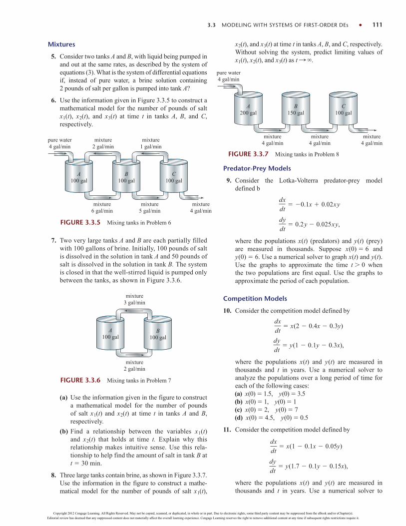
3.3 MODELING WITH SYSTEMS OF FIRST-ORDER DEs 111
Mixtures
5. Consider two tanks A and B, with liquid being pumped inand out at the same rates, as described by the system ofequations (3). What is the system of differential equationsif, instead of pure water, a brine solution containing2 pounds of salt per gallon is pumped into tank A?
6. Use the information given in Figure 3.3.5 to construct amathematical model for the number of pounds of saltx1(t), x2(t), and x3(t) at time t in tanks A, B, and C,respectively.
x2(t), and x3(t) at time t in tanks A, B, and C, respectively.Without solving the system, predict limiting values ofx1(t), x2(t), and x3(t) as t : .
mixture5 gal/min
mixture6 gal/min
mixture4 gal/min
pure water4 gal/min
B100 gal
C100 gal
A100 gal
mixture2 gal/min
mixture1 gal/min
FIGURE 3.3.5 Mixing tanks in Problem 6
7. Two very large tanks A and B are each partially filledwith 100 gallons of brine. Initially, 100 pounds of saltis dissolved in the solution in tank A and 50 pounds ofsalt is dissolved in the solution in tank B. The systemis closed in that the well-stirred liquid is pumped onlybetween the tanks, as shown in Figure 3.3.6.
mixture2 gal/min
mixture3 gal/min
B100 gal
A100 gal
FIGURE 3.3.6 Mixing tanks in Problem 7
(a) Use the information given in the figure to constructa mathematical model for the number of poundsof salt x1(t) and x2(t) at time t in tanks A and B,respectively.
(b) Find a relationship between the variables x1(t)and x2(t) that holds at time t. Explain why thisrelationship makes intuitive sense. Use this rela-tionship to help find the amount of salt in tank B att 30 min.
8. Three large tanks contain brine, as shown in Figure 3.3.7.Use the information in the figure to construct a mathe-matical model for the number of pounds of salt x1(t),
FIGURE 3.3.7 Mixing tanks in Problem 8
mixture4 gal/min
mixture4 gal/min
mixture4 gal/min
pure water4 gal/min
B150 gal
C100 gal
A200 gal
Predator-Prey Models
9. Consider the Lotka-Volterra predator-prey modeldefined b
,
where the populations x(t) (predators) and y(t) (prey)are measured in thousands. Suppose x(0) 6 and y(0) 6. Use a numerical solver to graph x(t) and y(t).Use the graphs to approximate the time t 0 whenthe two populations are first equal. Use the graphs toapproximate the period of each population.
Competition Models
10. Consider the competition model defined by
,
where the populations x(t) and y(t) are measured inthousands and t in years. Use a numerical solver toanalyze the populations over a long period of time foreach of the following cases:(a) x(0) 1.5, y(0) 3.5(b) x(0) 1, y(0) 1(c) x(0) 2, y(0) 7(d) x(0) 4.5, y(0) 0.5
11. Consider the competition model defined by
,
where the populations x(t) and y(t) are measured inthousands and t in years. Use a numerical solver to
dy
dt y(1.7 0.1y 0.15x)
dx
dt x(1 0.1x 0.05y)
dy
dt y(1 0.1y 0.3x)
dx
dt x(2 0.4x 0.3y)
dy
dt 0.2y 0.025xy
dx
dt 0.1x 0.02xy
Copyright 2012 Cengage Learning. All Rights Reserved. May not be copied, scanned, or duplicated, in whole or in part. Due to electronic rights, some third party content may be suppressed from the eBook and/or eChapter(s).
Editorial review has deemed that any suppressed content does not materially affect the overall learning experience. Cengage Learning reserves the right to remove additional content at any time if subsequent rights restrictions require it.

analyze the populations over a long period of time foreach of the following cases:(a) x(0) 1, y(0) 1(b) x(0) 4, y(0) 10(c) x(0) 9, y(0) 4(d) x(0) 5.5, y(0) 3.5
Networks
12. Show that a system of differential equations thatdescribes the currents i2(t) and i3(t) in the electricalnetwork shown in Figure 3.3.8 is
R1 di2
dt R2
di3
dt
1
C i3 0.
L di2
dt L
di3
dt R1i2 E(t)
112 CHAPTER 3 MODELING WITH FIRST-ORDER DIFFERENTIAL EQUATIONS
let s(t), i(t), and r(t) denote, in turn, the number of peo-ple in the community (measured in hundreds) who aresusceptible to the disease but not yet infected with it,the number of people who are infected with the dis-ease, and the number of people who have recoveredfrom the disease. Explain why the system of differen-tial equations
where k1 (called the infection rate) and k2 (called theremoval rate) are positive constants, is a reasonablemathematical model, commonly called a SIR model,for the spread of the epidemic throughout the commu-nity. Give plausible initial conditions associated withthis system of equations.
16. (a) In Problem 15, explain why it is sufficient toanalyze only
.
(b) Suppose k1 0.2, k2 0.7, and n 10. Choosevarious values of i(0) i0, 0 i0 10. Use anumerical solver to determine what the model pre-dicts about the epidemic in the two cases s0 k2k1
and s0 k2k1. In the case of an epidemic, estimatethe number of people who are eventually infected.
Project Problems
17. Concentration of a Nutrient Suppose compartmentsA and B shown in Figure 3.3.10 are filled with fluids andare separated by a permeable membrane. The figure isa compartmental representation of the exterior andinterior of a cell. Suppose, too, that a nutrient necessaryfor cell growth passes through the membrane. A model
di
dt k2i k1si
ds
dt k1si
dr
dt k2i,
di
dt k2i k1si
ds
dt k1si
R1E
i1 L i2i3
C
R2
FIGURE 3.3.8 Network in Problem 12
i1 i2
i3R1
R2 R3
E L1 L2
FIGURE 3.3.9 Network in Problem 13
13. Determine a system of first-order differential equationsthat describes the currents i2(t) and i3(t) in the electricalnetwork shown in Figure 3.3.9.
14. Show that the linear system given in (18) describesthe currents i1(t) and i2(t) in the network shown inFigure 3.3.4. [Hint: dqdt i3.]
Additional Nonlinear Models
15. SIR Model Acommunicable disease is spread through-out a small community, with a fixe population of n peo-ple, by contact between infected individuals and peoplewho are susceptible to the disease. Suppose that everyoneis initially susceptible to the disease and that no one leavesthe community while the epidemic is spreading. At time t,
FIGURE 3.3.10 Nutrient flow through a membrane iProblem 17
BA
membrane
fluid atconcentration
x(t)
fluid atconcentration
y(t)
Copyright 2012 Cengage Learning. All Rights Reserved. May not be copied, scanned, or duplicated, in whole or in part. Due to electronic rights, some third party content may be suppressed from the eBook and/or eChapter(s).
Editorial review has deemed that any suppressed content does not materially affect the overall learning experience. Cengage Learning reserves the right to remove additional content at any time if subsequent rights restrictions require it.

CHAPTER 3 IN REVIEW 113
solver to obtain numerical solution curves of (3) subjectto the initial conditions x1(0) 25, x2(0) 0.
20. Newton’s Law of Cooling/Warming As shown inFigure 3.3.11, a small metal bar is placed inside con-tainer A, and container A then is placed within a muchlarger container B. As the metal bar cools, the ambienttemperature TA(t) of the medium within container Achanges according to Newton’s law of cooling. Ascontainer A cools, the temperature of the medium in-side container B does not change significantly and canbe considered to be a constant TB. Construct a mathe-matical model for the temperatures T(t) and TA(t),where T(t) is the temperature of the metal bar insidecontainer A. As in Problems 1 and 18, this model canbe solved by using prior knowledge. Find a solution ofthe system subject to the initial conditions T(0) T0,TA(0) T1.
FIGURE 3.3.11 Container within a container in Problem 20
TA (t)
container A
container B
TB = constant
metalbar
for the concentrations x(t) and y(t) of the nutrient incompartments A and B, respectively, at time t is givenby the linear system of differential equations
,
where VA and VB are the volumes of the compartments,and k 0 is a permeability factor. Let x(0) x0 andy(0) y0 denote the initial concentrations of the nutri-ent. Solely on the basis of the equations in the systemand the assumption x0 y0 0, sketch, on the same setof coordinate axes, possible solution curves of the sys-tem. Explain your reasoning. Discuss the behavior ofthe solutions over a long period of time.
18. The system in Problem 17, like the system in (2), can besolved with no advanced knowledge. Solve for x(t) andy(t) and compare their graphs with your sketches inProblem 17. Determine the limiting values of x(t) andy(t) as t : . Explain why the answer to the last ques-tion makes intuitive sense.
19. Mixtures Solely on the basis of the physical descrip-tion of the mixture problem on page 107 and inFigure 3.3.1, discuss the nature of the functions x1(t)and x2(t). What is the behavior of each function over along period of time? Sketch possible graphs of x1(t) andx2(t). Check your conjectures by using a numerical
dy
dt
VB
(x y)
dx
dt
VA
(y x)
CHAPTER 3 IN REVIEW Answers to selected odd-numbered problems begin on page ANS-4.
Answer Problems 1 and 2 without referring back to the text.Fill in the blank or answer true or false.
1. If P(t) P0e0.15t gives the population in an environmentat time t, then a differential equation satisfied by P(t)is .
2. If the rate of decay of a radioactive substance isproportional to the amount A(t) remaining at time t, thenthe half-life of the substance is necessarily T (ln 2)k.The rate of decay of the substance at time t T is one-half the rate of decay at t 0.
3. In March 1976 the world population reached 4 billion.At that time, a popular news magazine predicted thatwith an average yearly growth rate of 1.8%, the worldpopulation would be 8 billion in 45 years. How does thisvalue compare with the value predicted by the modelthat assumes that the rate of increase in population isproportional to the population present at time t?
4. Air containing 0.06% carbon dioxide is pumped into aroom whose volume is 8000 ft3. The air is pumped in ata rate of 2000 ft3/min, and the circulated air is thenpumped out at the same rate. If there is an initial con-centration of 0.2% carbon dioxide in the room, deter-mine the subsequent amount in the room at time t. Whatis the concentration of carbon dioxide at 10 minutes?What is the steady-state, or equilibrium, concentrationof carbon dioxide?
5. Solve the differential equation
of the tractrix. See Problem 28 in Exercises 1.3. Assumethat the initial point on the y-axis in (0, 10) and that thelength of the rope is x 10 ft.
dy
dx y1s2 y2
Copyright 2012 Cengage Learning. All Rights Reserved. May not be copied, scanned, or duplicated, in whole or in part. Due to electronic rights, some third party content may be suppressed from the eBook and/or eChapter(s).
Editorial review has deemed that any suppressed content does not materially affect the overall learning experience. Cengage Learning reserves the right to remove additional content at any time if subsequent rights restrictions require it.

6. Suppose a cell is suspended in a solution containing asolute of constant concentration Cs. Suppose furtherthat the cell has constant volume V and that the area ofits permeable membrane is the constant A. By Fick’s law therate of change of its mass m is directly proportional to thearea A and the difference Cs C(t), where C(t) is the con-centration of the solute inside the cell at time t. Find C(t) ifm V C(t) and C(0) C0. See Figure 3.R.1.
114 CHAPTER 3 MODELING WITH FIRST-ORDER DIFFERENTIAL EQUATIONS
Find the current i(t) if the resistance is 0.2 ohm, theimpressed voltage is E(t) 4, and i(0) 0. Graph i(t).
10. A classical problem in the calculus of variations is tofind the shape of a curve such that a bead, under theinfluence of gravity, will slide from point A(0, 0) topoint B(x1, y1) in the least time. See Figure 3.R.2. It canbe shown that a nonlinear differential for the shape y(x)of the path is y[1 (y)2] k, where k is a constant.First solve for dx in terms of y and dy, and then use thesubstitution y k sin2u to obtain a parametric form ofthe solution. The curve turns out to be a cycloid.concentration
C(t)concentration
Cs
molecules of solutediffusing throughcell membrane
FIGURE 3.R.1 Cell in Problem 6
7. Suppose that as a body cools, the temperature of thesurrounding medium increases because it completelyabsorbs the heat being lost by the body. Let T(t) andTm(t) be the temperatures of the body and the mediumat time t, respectively. If the initial temperature of thebody is T1 and the initial temperature of the mediumis T2, then it can be shown in this case that Newton’slaw of cooling is dTdt k(T Tm), k 0, whereTm T2 B(T1 T ), B 0 is a constant.
(a) The foregoing DE is autonomous. Use the phaseportrait concept of Section 2.1 to determine thelimiting value of the temperature T (t) as t : .What is the limiting value of Tm(t) as t : ?
(b) Verify your answers in part (a) by actually solvingthe differential equation.
(c) Discuss a physical interpretation of your answers inpart (a).
8. According to Stefan’s law of radiation the absolutetemperature T of a body cooling in a medium at constantabsolute temperature Tm is given by
,
where k is a constant. Stefan’s law can be used over agreater temperature range than Newton’s law of cooling.
(a) Solve the differential equation.
(b) Show that when T Tm is small in comparison toTm then Newton’s law of cooling approximatesStefan’s law. [Hint: Think binomial series of theright-hand side of the DE.]
9. An LR-series circuit has a variable inductor with theinductance defined by
.L(t) 1
1
10t,
0,
0 t 10
t 10
dT
dt k(T 4 T 4
m )
FIGURE 3.R.2 Sliding bead in Problem 10
x
y
B(x1, y1)
A(0, 0)
bead
mg
11. A model for the populations of two interacting speciesof animals is
Solve for x and y in terms of t.
12. Initially, two large tanks A and B each hold 100 gallonsof brine. The well-stirred liquid is pumped between thetanks as shown in Figure 3.R.3. Use the informationgiven in the figure to construct a mathematical modelfor the number of pounds of salt x1(t) and x2(t) at time tin tanks A and B, respectively.
dy
dt k2xy.
dx
dt k1x ( x)
FIGURE 3.R.3 Mixing tanks in Problem 12
2 lb/gal7 gal/min
mixture5 gal/min
A100 gal
B100 gal
mixture3 gal/min
mixture1 gal/min
mixture4 gal/min
When all the curves in a family G(x, y, c1) 0 intersectorthogonally all the curves in another family H(x, y, c2) 0,the families are said to be orthogonal trajectories of eachother. See Figure 3.R.4. If dydx f (x, y) is the differentialequation of one family, then the differential equation for the
Copyright 2012 Cengage Learning. All Rights Reserved. May not be copied, scanned, or duplicated, in whole or in part. Due to electronic rights, some third party content may be suppressed from the eBook and/or eChapter(s).
Editorial review has deemed that any suppressed content does not materially affect the overall learning experience. Cengage Learning reserves the right to remove additional content at any time if subsequent rights restrictions require it.
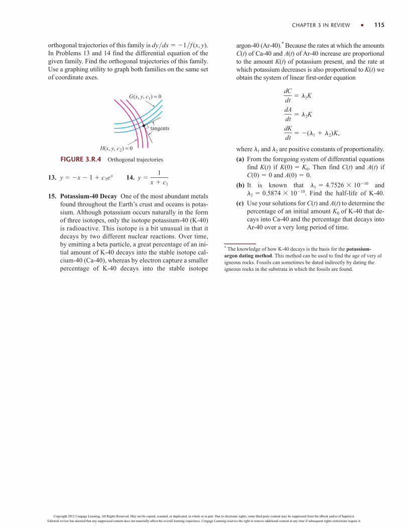
orthogonal trajectories of this family is dydx 1f (x, y).In Problems 13 and 14 find the differential equation of thegiven family. Find the orthogonal trajectories of this family.Use a graphing utility to graph both families on the same setof coordinate axes.
CHAPTER 3 IN REVIEW 115
FIGURE 3.R.4 Orthogonal trajectories
tangents
H(x, y, c2) = 0
G(x, y, c1) = 0
13. y x 1 c1ex 14.
15. Potassium-40 Decay One of the most abundant metalsfound throughout the Earth’s crust and oceans is potas-sium. Although potassium occurs naturally in the formof three isotopes, only the isotope potassium-40 (K-40)is radioactive. This isotope is a bit unusual in that itdecays by two different nuclear reactions. Over time,by emitting a beta particle, a great percentage of an ini-tial amount of K-40 decays into the stable isotope cal-cium-40 (Ca-40), whereas by electron capture a smallerpercentage of K-40 decays into the stable isotope
y 1
x c1
* The knowledge of how K-40 decays is the basis for the potassium-argon dating method. This method can be used to find the age of very oligneous rocks. Fossils can sometimes be dated indirectly by dating theigneous rocks in the substrata in which the fossils are found.
argon-40 (Ar-40).* Because the rates at which the amountsC(t) of Ca-40 and A(t) of Ar-40 increase are proportionalto the amount K(t) of potassium present, and the rate atwhich potassium decreases is also proportional to K(t) weobtain the system of linear first-order equation
where and are positive constants of proportionality.
(a) From the foregoing system of differential equationsfind if Then find and if
and
(b) It is known that andFind the half-life of K-40.
(c) Use your solutions for C(t) and to determine thepercentage of an initial amount of K-40 that de-cays into Ca-40 and the percentage that decays intoAr-40 over a very long period of time.
K0
A(t)
l2 0.5874 1010.l1 4.7526 1010
A(0) 0.C(0) 0A(t)C(t)K(0) K0.K(t)
l2l1
dK
dt (l1 l2)K,
dA
dt l2K
dC
dt l1K
Copyright 2012 Cengage Learning. All Rights Reserved. May not be copied, scanned, or duplicated, in whole or in part. Due to electronic rights, some third party content may be suppressed from the eBook and/or eChapter(s).
Editorial review has deemed that any suppressed content does not materially affect the overall learning experience. Cengage Learning reserves the right to remove additional content at any time if subsequent rights restrictions require it.