Review last lectures. procedures for drawing block diagram 1. Write the equations that describe the...
51
Review last lectures
-
date post
22-Dec-2015 -
Category
Documents
-
view
219 -
download
1
Transcript of Review last lectures. procedures for drawing block diagram 1. Write the equations that describe the...

Review last lectures
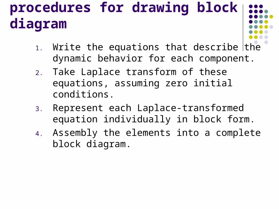
procedures for drawing block diagram
1. Write the equations that describe the dynamic behavior for each component.
2. Take Laplace transform of these equations, assuming zero initial conditions.
3. Represent each Laplace-transformed equation individually in block form.
4. Assembly the elements into a complete block diagram.
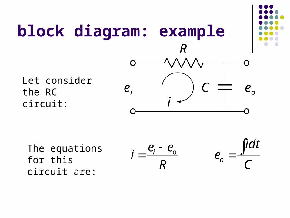
block diagram: example
Let consider the RC circuit:
R
Cei eoi
The equations for this circuit are: C
idte
R
eei o
oi

block diagram: exampletake Laplace transform:
R
sEsE
R
tetesI oioi )()()()()(
L
Cs
sI
C
idtsEo
L

block diagram: example
block representations for Laplace transforms:
R
sEsEsI oi )()()(
R
1_+
)(sI
sEo
)(sEi
Cs
sIsEo
Cs
1)(sI sEo

block diagram: exampleAssembly the elements into a complete block diagram.
R
1_+
)(sI
sEo
)(sEi
Cs
1)(sI sEo

block diagram reductionRules for reduction of the block diagram: Any number of cascaded blocks can be reduced by a
single block representing transfer function being a product of transfer functions of all cascaded blocks.
The product of the transfer functions in the feedforward direction must remain the same.
The product of the transfer functions around the loop mast remain the same.

block diagram: reduction example
R_+
_+1G 2G 3G
1H
2H
++
C
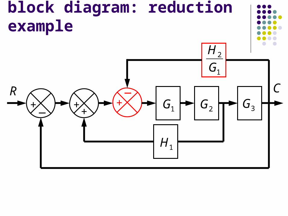
block diagram: reduction example
R_+
_+
1G 2G 3G
1H
1
2
G
H
++
C

block diagram: reduction example
R_+
_+
21GG 3G
1H
1
2
G
H
++
C
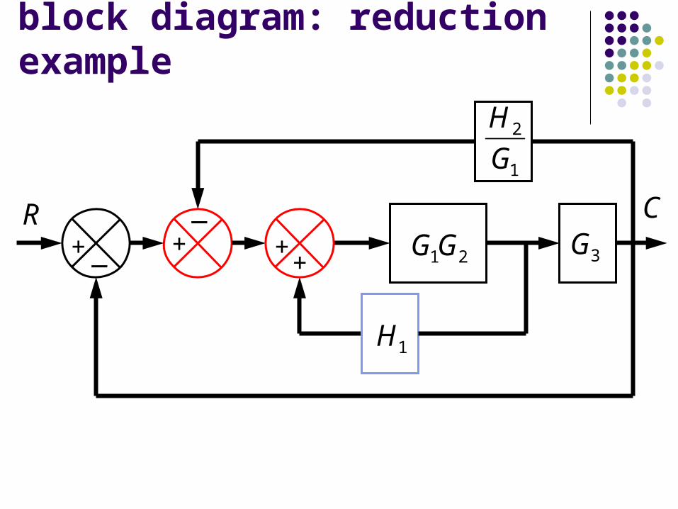
block diagram: reduction example
R_+
_+ 21GG 3G
1H
1
2
G
H
++
C
block diagram: reduction example
R_+
_+
121
21
1 HGG
GG
3G
1
2
G
H
C
block diagram: reduction example
R_+
_+
121
321
1 HGG
GGG
1
2
G
H
C
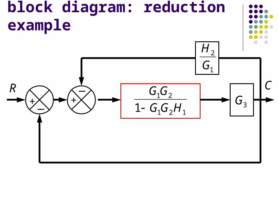
block diagram: reduction example
R_+
232121
321
1 HGGHGG
GGG
C
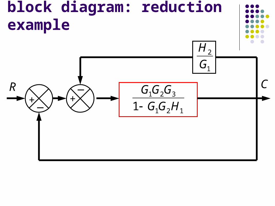
block diagram: reduction example
R
321232121
321
1 GGGHGGHGG
GGG
C
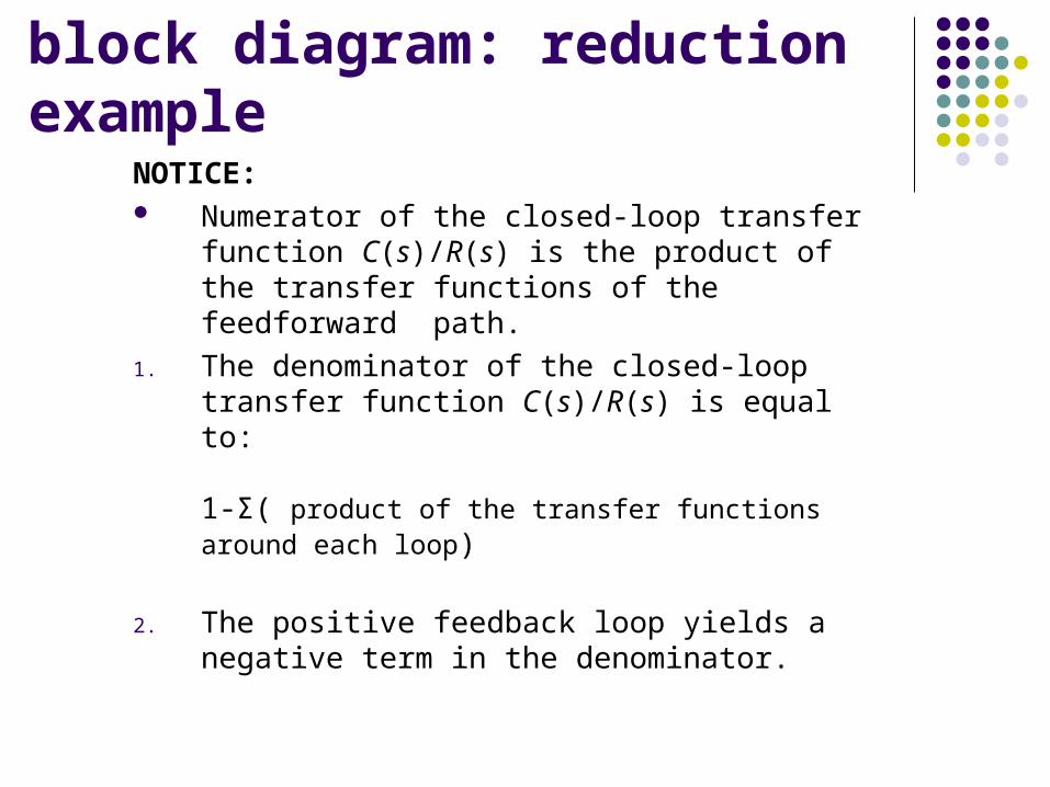
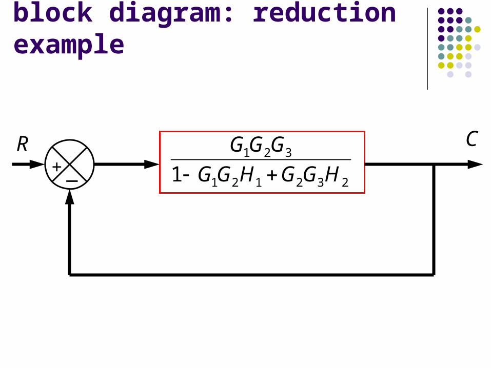
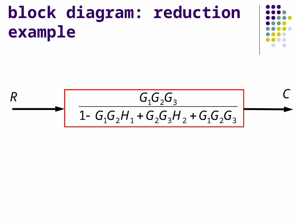
block diagram: reduction exampleNOTICE: Numerator of the closed-loop transfer function
C(s)/R(s) is the product of the transfer functions of the feedforward path.
1. The denominator of the closed-loop transfer function C(s)/R(s) is equal to:
1-Σ( product of the transfer functions around each loop)
2. The positive feedback loop yields a negative term in the denominator.

signal flow graph
input node (source)
b1x a
2x c
4x
d
1
3x
3x
output node (sink)
mixed node
input node (source)
mixed node
forward path
path
loop
branch
node
transmittance

flow graphs of control systems
)(sR)(sG
)(sC )(sG
)(sR )(sC
block diagram: signal flow graph:
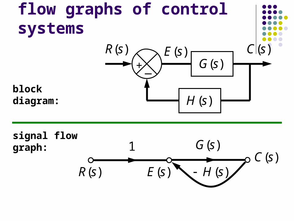
flow graphs of control systems)(sR
_+
)(sH
)(sG)(sC)(sE
block diagram:
signal flow graph:)(sG
)(sR)(sC
1
)(sE )(sH

flow graphs of control systems
)(sR
_+
)(sH
)(sG)(sC)(sE
block diagram:
signal flow graph:)(sG
)(sR )(sC
1
)(sE )(sH
++
)(sN
)(sN1
1)(sC
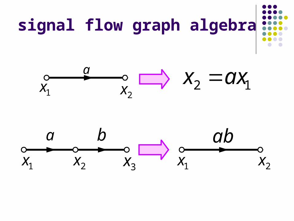
signal flow graph algebra
1xa
2x12 axx
b
1x
a
2x 3x 1x
ab
2x

signal flow graph algebra
b
a
2x
1x c
4x3xbc
ac
2x
1x
4x
1x
ba 2x
1x 2x
a
b

signal flow graph algebra
1xbc
ab
13x
1x 3xa bc
2x
ab1x
bc
3x
bc
ab
x
x
11
3
312
23
cxaxx
bxx
313 bcxabxx

flow graphs of linear systems113132121111 ubxaxaxax
223232221212 ubxaxaxax
3332321313 xaxaxax
3x
1x2x1
11u1b
12a
11a
13a
1x 3x2x
2u 2b23a
22a
21a
33a31a
32a

Transient and steady state response analyses
Input signal not known ahead of time but is random in nature!
In analyzing and designing we need basic comparison of performance so we need input signal by specifying particular test input signals.

Typical Test Signals
1. Step functions
2. Ramp functions
3. Acceleration (Parabolic) functions
4. Impulse functions
5. Sinusoidal functions
6. Polynomial functions
Note: which input signals we must use? Depend on the system normal operation inputs
ttf
ttf
function impulseUnit ,0 As
otherwise ,022
- ,/1

Test Input Signals
The impulse input is useful when we consider the convolution integral for the output y(t) in terms of an input r(t):
This relationship is shown in the block diagram:
If the input is a unit impulse function then
t
sRsGdttgty 1L
tgty

Transient response and Steady- State response
Time response parts Steady state
Output which behaves as t approach infinity
Transient
Which Goes from initial state to the final state
Or output minus steady state output!

First order systems response
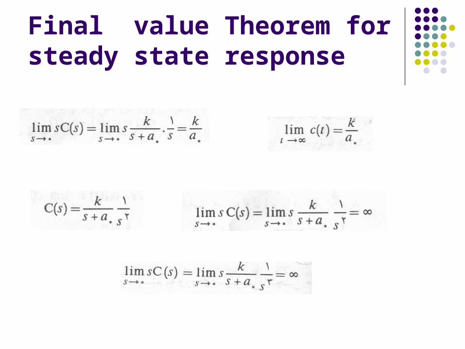
Final value Theorem for steady state response

Second order systems response(steady state part)
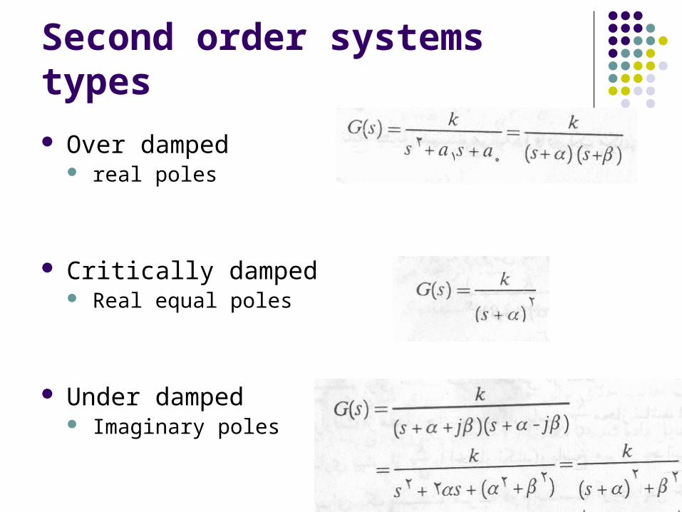
Second order systems types
Over damped real poles
Critically damped Real equal poles
Under damped Imaginary poles

Over damped response

Critically damped

Under damped

Under damped 2

Performance of a Second-Order System
Consider the system:
The closed loop output is:
22
2
22
2
2
2
input, stepunit aWith
2
Or
1
nn
n
nn
n
ssssY
sRss
sY
sRKpss
KsR
sG
sGsY
10 ,cos ,1
sin1
1
:isoutput transientThe
12
n
nt tety


UnstableStable

Performance of a Second-Order System The transient response of this second-order system is shown below. As ζ decreases, the closed-loop roots approach the imaginary axis,
and the response becomes oscillatory.
tety ntn 2
21sin
1
11:on Based

Performance of a Second-Order System For the unit impulse (R(s)=1) the output is:
The transient response is:
The impulse response of the
second order system is shown here
22
2
2 nn
n
sssY
tety ntn n 2
21sin
1
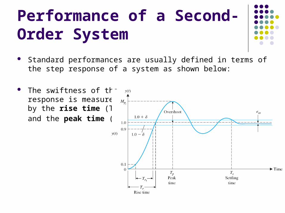
Performance of a Second-Order System Standard performances are usually defined in terms of the step
response of a system as shown below:
The swiftness of theresponse is measuredby the rise time (Tr),and the peak time (Tp).
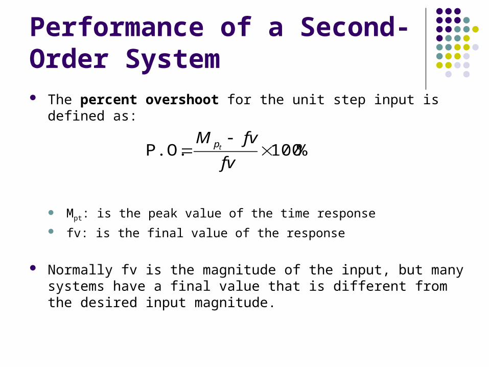
Performance of a Second-Order System The percent overshoot for the unit step input is defined as:
Mpt: is the peak value of the time response fv: is the final value of the response
Normally fv is the magnitude of the input, but many systems have a final value that is different from the desired input magnitude.
%100P.O.
fv
fvMtp
Performance of a Second-Order System
Settling time (Ts): the time required for the system to settle within a certain percentage, δ, of the input amplitude.
The settling time is four time constants (τ=1/ζωn) of the dominant roots of the characteristic equation.
The steady-state error of the system may be measured on the step response of the system as shown in the previous figure.

Performance of a Second-Order System Consider the second order system with closed-loop damping
constant ζωn and a response described by
We seek to determine the time, Ts, for which the response remains within 2% of the final value.
ns
sn
T
T
T
e sn
44
4
02.0
tety ntn 2
21sin
1
11

Performance of a Second-Order System
The transient response of the system may be described in terms of two factors: The swiftness of the response, as represented by
the rise time and the peak time The closeness of the response to the desired
response, as represented by the overshoot and settling time
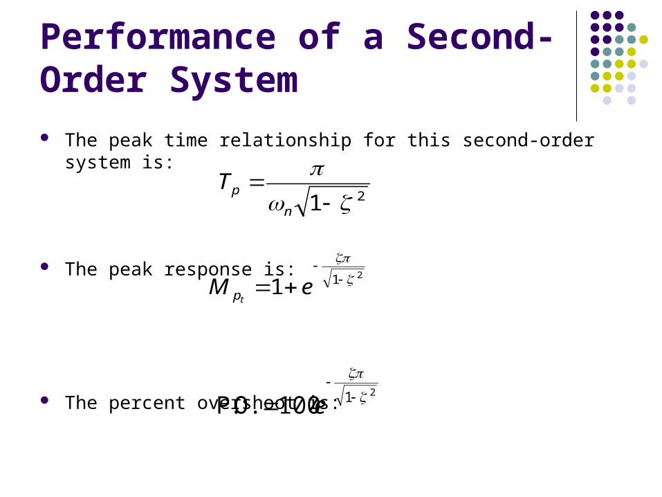
Performance of a Second-Order System The peak time relationship for this second-order system is:
The peak response is:
The percent overshoot is:
21
n
pT
211
eMtp
21100O..P
e

Performance of a Second-Order System The swiftness of step response can be measured as the time it takes to
rise from 10% to 90% of the magnitude of the step input. This is the rise time (Tr).
The swiftness of a response to a step input is dependent of ζ and ωn.
For a given ζ, the response is faster for larger ωn.
The overshoot is independent of ωn.
For a give ωn, the response is faster for lower ζ. The swiftness of the response will be limited by the overshoot that can
be accepted
rT 10 ,cos ,1 12 n

Quiz and Home work
Don’t forget quiz in next timeHome works of chapter 1 No: 1, 2, 3, 4, 5, 6, 7, 8, 13.