water

Article

Predicting the Specific Energy Consumption ofReverse Osmosis DesalinationAshlynn S. Stillwell 1,* and Michael E. Webber 2

1 Department of Civil and Environmental and Engineering, University of Illinois at Urbana-Champaign,Urbana, IL 61801, USA

2 Department of Mechanical Engineering, The University of Texas at Austin, Austin, TX 78712, USA;webber@mail.utexas.edu

* Correspondence: ashlynn@illinois.edu; Tel.: +1-217-244-6507

Academic Editors: Stephen Gray and Hideto MatsuyamaReceived: 23 September 2016; Accepted: 9 December 2016; Published: 16 December 2016

Abstract: Desalination is often considered an approach for mitigating water stress. Despite theabundance of saline water worldwide, additional energy consumption and increased costs presentbarriers to widespread deployment of desalination as a municipal water supply. Specific energyconsumption (SEC) is a common measure of the energy use in desalination processes, and dependson many operational and water quality factors. We completed multiple linear regression andrelative importance statistical analyses of factors affecting SEC using both small-scale meta-dataand municipal-scale empirical data to predict the energy consumption of desalination. Statisticallysignificant results show water quality and initial year of operations to be significant and importantfactors in estimating SEC, explaining over 80% of the variation in SEC. More recent initial year ofoperations, lower salinity raw water, and higher salinity product water accurately predict lowervalues of SEC. Economic analysis revealed a weak statistical relationship between SEC and costof water production. Analysis of associated greenhouse gas (GHG) emissions revealed importantconsiderations of both electricity source and SEC in estimating the GHG-related sustainability ofdesalination. Results of our statistical analyses can aid decision-makers by predicting the SEC ofdesalination to a reasonable degree of accuracy with limited data.

Keywords: desalination, greenhouse gas emissions, multiple linear regression, specific energyconsumption, statistical analysis

1. Introduction

Increasing stress on water supplies worldwide, coupled with population growth, has led manywater managers to seek alternative water sources to meet demand. Desalination of seawater orbrackish water is one such alternative water source, but it has important environmental, economic, andperformance tradeoffs [1]. For example, saline sources are abundant and drought-resistant. However,removing dissolved solids (salts) from saline water requires significantly more energy than is requiredfor treating conventional surface water or groundwater sources (see [2,3] and the sources cited thereinfor representative comparisons). There are other concerns, such as additional cost over conventionalwater supplies [4,5] and environmental impacts of concentrated salt and waste chemical disposal [6–8].Despite these concerns, worldwide desalination capacity continues to rise [9].

While desalination capacity is projected to increase globally [10], energy-water plannersand policymakers lack straightforward decision support tools that can help estimate the energyrequirements of new facilities with minimal site-specific data, for engaging community members indesalination conversations [11]. Full engineering designs typically include energy requirements as partof the plant specifications, yet those plans are usually completed late in the planning process. However,

Water 2016, 8, 601; doi:10.3390/w8120601 www.mdpi.com/journal/water

Water 2016, 8, 601 2 of 18

for many stakeholders, it would be valuable to understand the energy implications of different designconsiderations early in the process, before critical siting decisions and design specifications havebeen made. Unfortunately, based on personal conversations with policymakers, few such openlyaccessible easy-to-use tools exist for estimating energy requirements based on specific operationalparameters. Commercial membrane manufacturers offer desalination process modeling software,such as ROSA (Reverse Osmosis System Analysis) by Dow [12] and IMSDesign (Integrated MembraneSolutions Design) by Hydranautics [13], but these software packages require detailed inputs regardingoperations and water chemistry, which can be a knowledge barrier in early stage decision-making.Furthermore, because the performance depends on a wide range of operational parameters, the actualenergy requirements are a non-obvious result of many factors. This manuscript seeks to fill thatknowledge gap by use of a meta-regression analysis to create a predictive model of desalination’senergy requirements based on a range of relevant factors with minimal data inputs. It is the intent thatthis methodology would be useful for planners and decision-makers with publicly available data.

In the context of increasing desalination capacity and concern over energy consumption,we surveyed peer-reviewed desalination literature and the DesalData database by Global WaterIntelligence [14] and conducted statistical analyses to determine which operational factors mostinfluence the specific energy consumption (SEC)—that is, total desalination plant energy consumptionper unit volume of product water, measured in equivalent kWh/m3—of desalination processes.While published data are limited in terms of scope and specificity, we assembled a database fromvarious sources to reflect as many factors as plausible that we anticipate influence SEC of desalinationprocesses. Scientific- and statistically-based results pertaining to SEC and water cost are presented here ina policy-making context to better aid decision-making regarding future desalination plant installations.

2. Background

Historically, desalination has been confined to areas with scarce water resources and abundantenergy supplies needed to drive the desalting processes, such as the Middle East, or other isolatedisland communities. As the risk and reality of water scarcity faced other areas over time, desalinationcapacity increased worldwide in locations outside the Middle East as well, including the United States,Spain, Japan, and many others [9]. Worldwide desalination capacity has reportedly increased to a totalof nearly 87 million cubic meters per day (m3/day) as of 2015 [15].

Two primary technologies drive desalination operations: thermal and membrane processes.Thermal-based desalination uses energy in the form of heat (or removed heat in the case of freezedesalination) to separate water from dissolved solids. Common examples of thermal-based desalinationsystems include multi-stage flash (MSF), multiple effect distillation (MED), and multi-effect boiling(MEB) operations. Membrane-based desalination uses electricity to power high-pressure pumps feedingsemi-permeable membranes to filter out dissolved solids. Of the membrane-based desalinationtechnologies commercially available, reverse osmosis (RO) is the most common with applicationsin both seawater reverse osmosis (SWRO) and brackish water reverse osmosis (BWRO). In both thermal-and membrane-based desalination operations, the end result is a product water stream containing fewerdissolved solids and a concentrate waste stream containing more dissolved solids. With the developmentof membrane technologies, desalination operations gradually shifted from being primarily thermal-basedto more membrane-based, with 56% of the worldwide capacity and 96% of the United States capacityusing membrane technologies by 2006 [9]. Many innovative desalination technologies have emergedin recent years, including forward osmosis, humidification–dehumidification, membrane distillation,and others [16,17]; however, RO remains “the benchmark for comparison for any new desalinationtechnology” [18].

A substantial amount of the shift toward membrane-based desalination has been motivated bylower energy requirements, as shown by the equivalent SEC in Table 1. Here, we make the distinctionbetween thermal energy and electrical energy. While both are measured in kilowatt-hours (kWh), thetwo quantities are not directly comparable. To generate electrical energy (kWhe) in a typical thermal

Water 2016, 8, 601 3 of 18

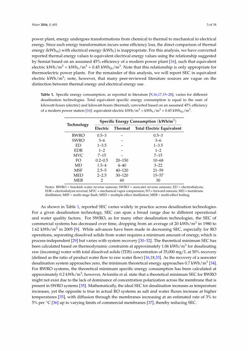
power plant, energy undergoes transformations from chemical to thermal to mechanical to electricalenergy. Since each energy transformation incurs some efficiency loss, the direct comparison of thermalenergy (kWhth) with electrical energy (kWhe) is inappropriate. For this analysis, we have convertedreported thermal energy values to equivalent electrical energy values using the relationship suggestedby Semiat based on an assumed 45% efficiency of a modern power plant [16], such that equivalentelectric kWh/m3 = kWhe/m3 + 0.45 kWhth/m3. Note that this relationship is only appropriate forthermoelectric power plants. For the remainder of this analysis, we will report SEC in equivalentelectric kWh/m3; note, however, that many peer-reviewed literature sources are vague on thedistinction between thermal energy and electrical energy use.

Table 1. Specific energy consumption, as reported in literature [9,16,17,19–28], varies for differentdesalination technologies. Total equivalent specific energy consumption is equal to the sum ofkilowatt-hours (electric) and kilowatt-hours (thermal), converted based on an assumed 45% efficiencyof a modern power station [16]: equivalent electric kWh/m3 = kWhe/m3 + 0.45 kWhth/m3.

TechnologySpecific Energy Consumption (kWh/m3)

Electric Thermal Total Electric Equivalent

BWRO 0.5–3 – 0.5–3SWRO 3–6 – 3–6

ED 1–3.5 – 1–3.5EDR 1–2 – 1–2MVC 7–15 – 7–15

FO 0.2–0.5 20–150 10–68MD 1.5–4 4–40 3–22MSF 2.5–5 40–120 21–59MED 2–2.5 30–120 15–57MEB 2 60 30

Notes: BWRO = brackish water reverse osmosis; SWRO = seawater reverse osmosis; ED = electrodialysis;EDR = electrodialysis reversal; MVC = mechanical vapor compression; FO = forward osmosis; MD = membranedistillation; MSF = multi-stage flash; MED = multiple effect distillation; MEB = multi-effect boiling.

As shown in Table 1, reported SEC varies widely in practice across desalination technologies.For a given desalination technology, SEC can span a broad range due to different operationaland water quality factors. For SWRO, as for many other desalination technologies, the SEC ofcommercial systems has decreased over time, dropping from an average of 20 kWh/m3 in 1980 to1.62 kWh/m3 in 2005 [9]. While advances have been made in decreasing SEC, especially for ROoperations, separating dissolved solids from water requires a minimum amount of energy, which isprocess-independent [29] but varies with system recovery [30–32]. The theoretical minimum SEC hasbeen calculated based on thermodynamic constraints at approximately 1.06 kWh/m3 for desalinatingraw (incoming) water with total dissolved solids (TDS) concentration of 35,000 mg/L at 50% recovery(defined as the ratio of product water flow to raw water flow) [16,18,33]. As the recovery of a seawaterdesalination system approaches zero, the minimum theoretical energy approaches 0.7 kWh/m3 [34].For BWRO systems, the theoretical minimum specific energy consumption has been calculated atapproximately 0.2 kWh/m3; however, Avlonitis et al. state that a theoretical minimum SEC for BWROmight not exist due to the lack of dominance of concentration polarization across the membrane that ispresent in SWRO systems [35]. Mathematically, the ideal SEC for desalination increases as temperatureincreases, yet the opposite is true in actual RO systems as salt and water fluxes increase at highertemperatures [35], with diffusion through the membranes increasing at an estimated rate of 3% to5% per ◦C [36] up to varying limits of commercial membranes [37], thereby reducing SEC.

Water 2016, 8, 601 4 of 18

Many operational and water quality factors can influence SEC for a given desalinationtechnology [38–40]. For example, RO facilities with larger treatment capacity often observe economiesof scale in terms of SEC due to efficiency gains associated with larger pumps [16]. Similarly, useof energy recovery technologies can substantially reduce the SEC of membrane-based desalination;however, the capital costs of such systems can be prohibitively expensive for small-scale SWRO(<100 m3/day capacity) [41]. In SWRO applications, Pelton turbines (typical energy savings of 35% to42% compared to a baseline without energy recovery equipment) for energy recovery are generallyapplicable for ≤5000 m3/day capacity, while isobaric energy recovery devices (typical energy savingsof 55% to 60%) are suited for >5000 m3/day [42]. Approaches to reduce SEC include use of highpermeability membranes [43], use of energy recovery devices, intermediate chemical demineralization,use of renewable energy, and optimal process configuration [44]. With advanced materials, increasedwater-solute selectivity has become more important than additional increases in water permeability,since increasing permeability negligibly decreases SEC [45–47]. Since reported energy consumptiontypically represents 19% to 44% of the cost of desalination [16,23,25,48–50], understanding whichfactors most significantly affect the SEC of desalination processes becomes important for the futureenvironmental and social sustainability of desalination as an alternative water source.

3. Methodology

To determine the significance level of factors affecting SEC for desalination processes, we completedmultiple linear regression analyses of SEC and cost as a function of various factors. The general form ofthe model is shown in Equation (1):

y = β0 + β1x1 + β2x2 + β3x3 + . . . + βnxn + ε (1)

where y represents the dependent variable (in this case, SEC or cost), each xi (for i = 1 . . . n) isan independent explanatory variable, and each βi (for i = 0 . . . n) is a best-fit coefficient such that theerror term ε is minimized. The use of multiple linear regression statistical techniques assumes certaincharacteristics about the model and the data on which it is based. In particular, statistical hypothesistesting is recommended to examine significance of individual coefficients, overall model significance,equality of two or more coefficients, satisfaction of restrictions for regression coefficients, stability ofthe model over time, and the functional form of the model [51].

We used the open-source statistical program R to create our multiple linear regression models.Based on the hypothesis tests for multiple linear regression given in Gujarati [51], we criticallyexamined our model results to check for each of the following criteria:

1. Significance of individual coefficients2. Overall model significance3. No (or little) multicollinearity4. No (or little) heteroscedasticity5. No (or little) autocorrelation.

The presence of multicollinearity, often quantified with a variance inflation factor, indicates a linearrelationship between two or more explanatory variables xi, which are assumed to be independent.For example, the product water flow rate, qpw, and the raw water flow rate, qrw, are related to eachother via the recovery, R, as the ratio between the two explanatory variables. Consequently, somemulticollinearity is expected between qrw and qpw. Some suggest, however, that since “sometimeswe have no choice over the data we have available for empirical analysis,” a certain degree ofmulticollinearity is not detrimental to a regression model if the model’s objective is predictiveonly [51]. Heteroscedasticity and autocorrelation are indications of non-constant variance and serialcorrelation (trending) among the model residual values (i.e., the difference between observed andpredicted values), respectively. Significant heteroscedasticity and autocorrelation would indicatean inappropriate statistical model formulation (e.g., linear model versus non-linear model).

Water 2016, 8, 601 5 of 18

We completed the statistical analyses of SEC and cost using two distinct datasets: (1) data collectedfrom published literature representing small-scale (product water flow: 0.7 to 220 m3/day) desalinationsystems; and (2) data reported in the DesalData database representing municipal-scale (product waterflow: 2500 to 368,000 m3/day) systems. The small-scale database contained SEC data of desalinationprocesses reported in peer-reviewed literature published since 2000 [16,19–22,27,35,36,41,42,52–61],including information for the raw water flow rate qrw (m3/day), product water flow rate qpw (m3/day),recovery R (unitless), year YR, raw water TDS crw (mg/L), product water TDS cpw (mg/L), operating(feed) pressure P (bar), energy recovery ER (binary variable, unitless), and temperature T (◦C).These desalination factors, summarized in Table 2, represented the explanatory variables in ourmultiple linear regression model for small-scale desalination facilities, referred to here as the small-scalemodel. Recovery was included as “inverse recovery” in the models as 1

1−R since SEC is proportionalto this value [40,47]. The use of energy recovery systems was included as a binary variable with 0indicating no energy recovery technology and 1 indicating the use of at least one energy recovery device,since the amount of energy savings is not often reported and different energy recovery technologiessave similar percentages of operational energy [42]. For literature data where no raw water TDSvalues were reported, we assumed values of 35,000 mg/L for seawater and 10,000 mg/L for brackishwater. Note that while many literature sources include some data on SEC of thermal desalinationprocesses, our database (n = 45) included only RO membrane-based technologies due to the statisticalrequirement for complete datasets when employing multiple linear regression techniques.

Table 2. Different desalination factors, with ranges in observed values as noted, were used asexplanatory variables in the small-scale and municipal-scale models of specific energy consumption.

Factor Units Small-Scale Model Municipal-Scale Model

Year of initial operations N/A 2003–2015 1988–2012Raw water TDS mg/L 1000–40,000 400–52,000Product water TDS mg/L 6–1632 10–500Raw water flow rate m3/day 2.04–600 –Product water flow rate m3/day 0.696–220.4 –Recovery N/A 0.04–0.81 –Pressure bar 4–71 –Energy recovery * N/A 0, 1 –Temperature ◦C 18–35 –

Note: * Binary variable.

The municipal-scale database contained SEC data of desalination processes reported in theDesalData database from Global Water Intelligence [14], reflecting actual operations at desalinationfacilities worldwide. Although the DesalData database is extensive in its reporting with informationon over 18,000 facilities, several parameters are either not requested by Global Water Intelligence or notreported by the desalination plants, with 74 facilities reporting SEC. Consequently, our municipal-scaledatabase (n = 36) contained SEC data including year YR, raw water TDS crw (mg/L), and productwater TDS cpw (mg/L) only, to maintain complete datasets.

Based on literature, energy consumption is a non-negligible determinant of the cost of desalinatedwater, representing as much as 44% of costs [16,23,48–50]. To quantify the statistical significance ofSEC related to desalination economics, we completed an economic statistical analysis consideringboth product water cost ppw ($/m3) and engineering-procurement-construction (EPC) price pEPC ($)based on data from the DesalData database. As a small data sample (n = 16 for ppw; n = 28 for pEPC),these cost data give a limited yet robust view of desalinated water economics.

Water 2016, 8, 601 6 of 18

To complement the multiple linear regression models of the small-scale and municipal-scaledatabases, we performed relative importance analyses of the coefficient estimates based on thetechnique presented by Tomidandel and LeBreton [62]. Relative importance analysis partitions thevariance explained by a multiple linear regression model among the predictors (i.e., βi’s) such thatthe relative importance weights of the coefficients sum to the model’s R2 value. Since “standardizedregression weights do not appropriately partition variance when predictors are correlated,” relativeimportance analysis is one approach to coping with multicollinearity challenges [62]. We completedthe relative importance analyses of factors in our small-scale and municipal-scale databases usinga customized version of R code available from Tomidandel and LeBreton [63].

Because desalination is an energy-intensive process, its operation often causes the emission ofgreenhouse gases (GHGs). These GHG emissions associated with electricity consumption vary in timeand space, as different electricity grids rely on different fuels with different associated GHG emissions.To quantify the GHG emissions from SEC at modeled desalination operations, we used empiricalSEC and GHG data for U.S. desalination facilities to geographically represent the air emissions frommajor desalination plants. The resulting GHG analysis represents a first-order quantification of GHGemissions from electricity consumption for desalination; higher order impacts, such as GHG emissionsassociated with chemical consumption, infrastructure materials, or other operations, are excluded inthis estimate.

4. Results

The results of our multiple linear regression and relative importance statistical analyses arepresented here, first for the small-scale and municipal-scale desalination models of SEC, followed byeconomic analysis of product water cost and EPC price.

4.1. Small-Scale Desalination Operations Model

Using literature data on small-scale (0.7 m3/day ≤ qpw ≤ 220 m3/day; n = 45) desalinationoperations, we created a multiple linear regression model of SEC as a function of eight independentvariables: raw water flow, product water flow, inverse recovery, raw water TDS, product water TDS,pressure, energy recovery equipment, and temperature. A summary of the results of our multiplelinear regression model for small-scale desalination operations is shown in Table 3 and illustrated inFigure 1. Three values in our small-scale dataset were determined to be outliers based on Rosner’soutlier test [64] and were subsequently excluded from the analysis.

Using the five previously mentioned statistical criteria to evaluate the multiple linear regressionmodel, we can state the following:

1. Significance of individual coefficientsAt a significance level (i.e., Pr(>|t|)) of 0.05 as is commonly accepted in statistical analysis, all ofthe individual coefficients of the small-scale model are considered statistically significant sincePr(>|t|) ≤ 0.05. Since we are making a hypothesis test regarding significance for each coefficient,the value of Pr(>|t|) is essentially the probability of observing the estimated value by chance.A lower value of Pr(>|t|) indicates a more statistically significant estimate.

2. Overall model significanceAgain using the significance level of 0.05, the small-scale model is highly significant with a p-valueof 1.1 × 10−12. Additionally, the multiple R2 value of 0.85 indicates that approximately 85% of thevariation in SEC can be explained by the multiple linear regression model, making the coefficientestimates a good model fit in predicting SEC.

3. Limited multicollinearityBased on rules of thumb [51], multicollinearity is said to exist when the variance inflation factor(VIF) for a given explanatory variable is greater than 10. In our small-scale model of desalinationoperations, some strong multicollinearity exists with the explanatory variables for raw waterflow rate, product water flow rate, raw water TDS, and pressure, as given in the Appendix A,

Water 2016, 8, 601 7 of 18

Table A1. For this predictive analysis, we have not attempted to correct for multicollinearitydue to data limitations and, rather, have taken the “do nothing” approach suggested by somestatisticians [51].

4. Limited heteroscedasticityThe residual plots of each of the explanatory variables in our small-scale model, shown in theAppendix A, Figure A1, show some unequal variance across the sample size, indicated by thevertical spread of the residual data. With limited data reported in literature, we proceeded withthe heteroscedasticity present in the small-scale model.

5. No (or little) autocorrelationIn the residual plots shown in the Appendix A, Figure A1, no observable trend is present for eachof the variables in our model of desalination factors, indicating no autocorrelation.

Table 3. Multiple linear regression results for the small-scale model of desalination operations (n = 45)revealed a reasonable model fit with highly significant coefficients. Values have been rounded to twosignificant figures.

Factor Variable Coefficient Estimate Standard Error t-Value Pr(>|t|)Constant β0 7.7 1.2 6.2 3.8 × 10−7

Raw water flow (m3/day) qrw β1 3.9 × 10−2 5.3 × 10−3 7.3 1.4 × 10−8

Product water flow (m3/day) qpw β2 −8.6 × 10−2 1.5 × 10−2 −5.9 9.7 × 10−7

Inverse recovery 11−R β3 1.7 0.21 8.0 1.5 × 10−9

Raw water TDS (mg/L) crw β4 6.2 × 10−4 9.6 × 10 −5 6.4 2.0 × 10−7

Product water TDS (mg/L) cpw β5 4.2 × 10−3 1.7 × 10−3 2.5 1.7 × 10−2

Pressure (bar) P β6 −0.34 6.0 × 10−2 −5.7 2.0 × 10−6

Energy recovery equipment ER β7 −5.4 0.72 −7.6 5.9 × 10−9

Temperature (◦C) T β8 −0.20 4.5 × 10−2 −4.5 6.5 × 10−5

multiple R2 = 0.85; adjusted R2 = 0.82; F-statistic = 26 (p-value = 1.1 × 10−12)

With many explanatory variables in the small-scale model, we applied relative importanceanalysis (from Tonidandel and LeBreton [62]) to estimate the relative weight, or the amount of variancein SEC that is explained, for each variable. The relative weights sum to the R2 value. These results aresummarized in Table 4. When considering statistical significance along with relative weight, waterquality parameters (crw and cpw), pressure, and use of energy recovery equipment emerge as themost important variables in predicting SEC. Although the remaining four factors in the small-scalemodel each explain some amount of the variation in SEC, as observed by the relative weights inTable 4, a majority of the modeled SEC is explained by water quality, pressure, and energy recoveryequipment alone.

Table 4. Relative importance analysis results for the small-scale model of desalination operations(n = 45) revealed a strong dependence on water quality, pressure, and use of energy recovery equipment.Values have been rounded to two significant figures.

Factor Variable Relative Weight

Raw water flow (m3/day) qrw 0.067 *Product water flow (m3/day) qpw 0.072 *Inverse recovery 1

1−R 0.071 *Raw water TDS (mg/L) crw 0.15 *Product water TDS (mg/L) cpw 0.19 *Pressure (bar) P 0.12 *Energy recovery equipment ER 0.15 *Temperature (◦C) T 0.034

Note: * relative weight is statistically significant.

Water 2016, 8, 601 8 of 18

Based on the multiple linear regression evaluation criteria and relative importance analysis,our model of small-scale desalination operations is a good statistical fit of the data with predictivecapabilities, depending heavily on water quality, pressure, and use of energy recovery equipment.Figure 1 illustrates the observed data as it aligns with the predicted SEC using our multiple linearregression model. While the model overestimates some observed values and underestimates others,the overall model fit is reasonable and appropriate for future use regarding SEC for small-scale(0.7 m3/day ≤ qpw ≤ 220 m3/day) membrane-based desalination processes.

0 5 10 15

05

1015

Observed vs. Predicted Specific Energy Consumption

Predicted SEC (kWh/m3)

Obs

erve

d S

EC

(kW

h/m3 )

Small-Scale Model (product flow: 0.7 to 220 m3/day); n = 45

Figure 1. Our model for small-scale desalination operations predicts energy consumption consistentwith observed energy consumption.

4.2. Municipal-Scale Desalination Operations Model

The DesalData database from Global Water Intelligence [14] is an extensive repository of datafrom current and proposed desalination facilities worldwide. Reported data include facility location,technology, suppliers, source water, operational characteristics, and other data. Using operationaldata from DesalData for municipal-scale (2500 m3/day ≤ qpw ≤ 368,000 m3/day; n = 36) desalinationoperations, we created a multiple linear regression model of SEC as a function of the three mostcomplete explanatory variables available in the DesalData database: initial year of operations, rawwater TDS, and product water TDS. Two values in our municipal-scale dataset were excluded from theanalysis since they reported values below the minimum theoretical energy consumption. A summaryof the results of our multiple linear regression model for municipal-scale desalination operations isshown in Table 5 and illustrated in Figure 2. Using the five previously mentioned statistical criteria toevaluate the multiple linear regression model, we can state the following:

1. Significance of individual coefficientsAt a significance level of 0.05, all of the individual coefficients, including the constant, areconsidered statistically significant in the municipal-scale model, as shown in Table 5.

2. Overall model significanceAgain using the significance level of 0.05, the municipal-scale model is significant with a p-value of5.5 × 10−14. In addition to the model’s significance, the multiple R2 value of 0.86 indicates thatapproximately 86% of the variation in SEC can be explained by the variables in the multiple linearregression model, making the coefficient estimates a strong model fit in predicting SEC.

Water 2016, 8, 601 9 of 18

3. No (or little) multicollinearityIn our municipal-scale model, no multicollinearity exists in the explanatory variables, as shown bythe VIFs less than 10 in the Appendix A, Table A2.

4. No (or little) heteroscedasticityThe residual plots of each of the explanatory variables in our municipal-scale model, shown in theAppendix A, Figure A2, show minor heteroscedasticity with relatively constant variance acrossthe dataset.

5. No (or little) autocorrelationIn the residual plots shown in the Appendix A, Figure A2, negligible, if any, observable trends arepresent for the variables in our municipal-scale model.

Table 5. Multiple linear regression results for the municipal-scale model of desalination operations(n = 36) revealed a reasonable model fit with highly significant coefficients. Values have been roundedto two significant figures.

Factor Variable Coefficient Estimate Standard Error t-Value Pr(>|t|)Constant β0 260 35 7.5 1.4 × 10−8

Year of initial operations YR β1 −0.13 1.7 × 10−2 −7.5 1.5 × 10−8

Raw water TDS (mg/L) crw β2 8.3 × 10−5 8.4 × 10−6 9.8 3.5 × 10−11

Product water TDS (mg/L) cpw β3 −2.4 × 10−3 7.1 × 10−4 −3.4 2.0 × 10−3

multiple R2 = 0.86; adjusted R2 = 0.85; F-statistic = 68 (p-value = 5.5 × 10−14)

0 1 2 3 4 5 6 7

01

23

45

67

Observed vs. Predicted Specific Energy Consumption

Predicted SEC (kWh/m3)

Obs

erve

d S

EC

(kW

h/m3 )

Municipal-Scale Model (product flow: 2500 to 368,000 m3/day); n = 36

Figure 2. Our model for municipal-scale desalination operations predicts energy consumptionconsistent with observed energy consumption.

Unlike the small-scale model, our municipal-scale model depends on only three explanatoryvariables. We performed a relative importance analysis for the municipal-scale model to estimatethe distribution of importance between these three variables, as shown in Table 6. Of the threeexplanatory variables in the municipal-scale model, the relative weights of all of the factors werefound to be significant. Two factors—year of initial operations, YR, and raw water TDS, crw—togetherexplain over 80% of the variation in SEC in the municipal-scale model. Product water TDS, cpw, has

Water 2016, 8, 601 10 of 18

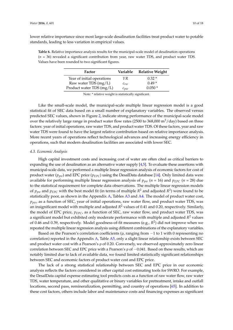
lower relative importance since most large-scale desalination facilities treat product water to potablestandards, leading to less variation in empirical values.

Table 6. Relative importance analysis results for the municipal-scale model of desalination operations(n = 36) revealed a significant contribution from year, raw water TDS, and product water TDS.Values have been rounded to two significant figures.

Factor Variable Relative Weight

Year of initial operations YR 0.32 *Raw water TDS (mg/L) crw 0.49 *

Product water TDS (mg/L) cpw 0.050 *

Note: * relative weight is statistically significant.

Like the small-scale model, the municipal-scale multiple linear regression model is a goodstatistical fit of SEC data based on a small number of explanatory variables. The observed versuspredicted SEC values, shown in Figure 2, indicate strong performance of the municipal-scale modelover the relatively large range in product water flow rates (2500 to 368,000 m3/day) based on threefactors: year of initial operations, raw water TDS, and product water TDS. Of these factors, year and rawwater TDS were found to have the largest relative contribution based on relative importance analysis.More recent years of operations reflect technological advances and increasing energy efficiency inoperations, such that modern desalination facilities are associated with lower SEC.

4.3. Economic Analysis

High capital investment costs and increasing cost of water are often cited as critical barriers toexpanding the use of desalination as an alternative water supply [4,5]. To evaluate these assertions withmunicipal-scale data, we performed a multiple linear regression analysis of economic factors for cost ofproduct water (ppw) and EPC price (pEPC) using the DesalData database [14]. Only limited data wereavailable for performing multiple linear regression analysis of ppw (n = 16) and pEPC (n = 28) dueto the statistical requirement for complete data observations. The multiple linear regression modelsof ppw and pEPC with the best model fit (in terms of multiple R2 and adjusted R2) were found to bestatistically poor, as shown in the Appendix A, Tables A3 and A4. The model of product water cost,ppw, as a function of SEC, year of initial operations, raw water flow, and product water TDS, wasan insignificant model with multiple and adjusted R2 values of 0.41 and 0.20, respectively. Similarly,the model of EPC price, pEPC, as a function of SEC, raw water flow, and product water TDS, wasa significant model but exhibited only moderate performance with multiple and adjusted R2 valuesof 0.46 and 0.39, respectively. Model goodness-of-fit measures (e.g., R2) did not improve when werepeated the multiple linear regression analysis using different combinations of the explanatory variables.

Based on the Pearson’s correlation coefficients (ρ, ranging from −1 to 1 with 0 representing nocorrelation) reported in the Appendix A, Table A5, only a slight linear relationship exists between SECand product water cost with a Pearson’s ρ of 0.20. Conversely, we observed approximately zero linearcorrelation between SEC and EPC price with a Pearson’s ρ of −0.041. Based on these results, which arenotably limited due to lack of available data, we found limited statistically significant relationshipsbetween SEC and economic factors of product water cost and EPC price.

The lack of a strong statistical relationship between SEC and EPC price in our economicanalysis reflects the factors considered in other capital cost estimating tools for SWRO. For example,the DesalData capital expense estimating tool predicts costs as a function of raw water flow, raw waterTDS, water temperature, and other qualitative or binary variables for pretreatment, intake and outfalllocations, second pass, remineralization, permitting, and country of operations [65]. In addition tothese cost factors, others include labor and maintenance costs and financing expenses as significant

Water 2016, 8, 601 11 of 18

considerations [23,50]. Energy consumption is typically a significant factor in operations, but is notnecessarily a direct factor in capital equipment cost.

5. Policy and Sustainability Implications

High electricity requirements for RO operations often translate into high associated GHGemissions. Since many U.S. electricity and GHG policy decisions are state-based, we quantifiedthe GHG emissions (as carbon dioxide equivalent, CO2e) associated with selected desalination facilitiesnationwide, as shown in Figure 3. Since different locations utilize a different mix of electricity fuels(with different associated GHG emissions), electricity consumption and GHG emissions producedin one facility are not necessarily reflective of another site. For example, electricity generated inCalifornia produces fewer GHG emissions on average than electricity generated in Texas. Consequently,SWRO operations in California (with higher SEC) have lower associated GHG emissions per unit ofdesalinated water than BWRO operations in Texas (with lower SEC).

Specific Energy ConsumptionScale:

Electricity Generation (by fuel):

kWh/m30.68

Coal Natural Gas Nuclear Hydro Renewables Other

0 250 500125km±

Original analysis by Stillwell and Webber (2016), based on state-level data from the U.S. Environmental Protection Agency, Energy Information Administration, and DesalData.com. mtCO2e = metric ton carbon dioxide equivalent.

ChandlerDesalination Facility

Chandler, AZ9,090 m3/day

6,200 mtCO2e/year

Kay Bailey HutchinsonDesalination Facility

El Paso, TX106,000 m3/day

36,000 mtCO2e/year

Layne ChristensenDesalination Pilot

Phoenix, AZ200 m3/day

21 mtCO2e/year

Tampa BayDesalination Facility

Tampa Bay, FL109,000 m3/day

56,000 mtCO2e/year

Geneva WaterTreatment Facility

Geneva, IL30,000 m3/day

6,100 mtCO2e/year

BarstowDesalination Facility

Barstow, CA600 m3/day

210 mtCO2e/year

Huntington BeachDesalination FacilityHuntington Beach, CA

189,000 m3/day53,000 mtCO2e/year

OceansideDesalination Facility

Oceanside, CA15,000 m3/day

5,100 mtCO2e/year

Figure 3. Greenhouse gas emissions associated with electricity consumption for desalination varywith location in selected U.S. desalination facilities. Larger circles correspond to higher specificenergy consumption.

In response to severe and on-going drought, cities in California have renewed interest inseawater desalination as a water source; however, energy requirements, environmental impacts,and costs continue to be cited as criticisms. Some view desalination as a risky option when plants areconstructed before strong demand exists, yet others view desalination plant construction as a long-terminfrastructure investment [66]. Based on our statistical analysis of SEC and associated GHG emissions,desalination in California might lead to fewer GHG emissions than similarly sized operations elsewheredue to the lower CO2e emissions from California-generated electricity.

The GHG emissions associated with water-related energy reveal the importance of droughtmanagement and water conservation as an approach to reducing CO2e emissions under variousstate and federal emission policies. Using our municipal-scale multiple linear regression model,we estimated SEC for the recently-opened Carlsbad Desalination Project in southern California tobe SECCarlsbad = 3.5 ± 0.23 kWh/m3, with the statistical uncertainty estimate successfully predicting

Water 2016, 8, 601 12 of 18

the reported (likely conservative) SEC value of 3.6 kWh/m3 [67]. Based on the model by Stokes andHorvath [68] of electricity and associated GHG emissions for water in southern California, replacingthe current imported water supply in southern California with desalinated water from the Carlsbadfacility would increase electricity consumption by a factor of 2.1. Consequently, a target reductionin municipal water use of over 53% is necessary to avoid increasing GHG emissions in response tosubstituting desalination for the baseline water supplies in southern California. This target reductionpercentage might notably decrease over time given the observed trend of increasing cost (both interms of economics and energy) of marginal water withdrawal and decreasing cost of desalinationand reuse [50]. Integrating desalination operations with renewable electricity generation [1,69–71] isanother option to increase the sustainability of desalination.

6. Model Limitations

The small-scale and municipal-scale models demonstrate strong statistical goodness-of-fitmeasures (e.g., R2, model F-statistic) for predicting SEC in RO desalination; however, these models areempirical and depend on the underlying data. As such, the trends are reflective of the data range underconsideration. Caution should be exercised in extrapolating SEC results. SEC has generally decreasedover time [9], but the theoretical minimum of 1.06 kWh/m3 (for crw = 35,000 mg/L and R = 0.50)constrains the lower bounds [16,18,33]. Actual RO operations are not reversible thermodynamicprocesses such that SEC is larger than the theoretical minimum [18]. Extrapolating input data, such asinitial year of operations or raw water TDS, outside the bound of the empirical data, shown in Table 2,can lead to misleading and incorrect values of SEC.

Although we have compiled a thorough database with information on many desalination factorsaffecting SEC for both small- and municipal-scale operations, our database is not exhaustive of all thefactors that affect energy use in desalination processes. Comparing the small-scale and municipal-scalemodels, fewer explanatory variables are necessary to predict SEC at the municipal-scale; however,a limited number of variables can miss important factors in a modeling and prediction effort.In particular, very little data were available regarding management of concentrate waste streams,which can affect overall facility sustainability and energy consumption. For inland RO facilities,management and disposal of concentrated dissolved solids and waste chemical streams can bea significant factor influencing overall energy consumption and desalination cost since inland facilitieshave limited disposal options, including evaporation ponds, zero liquid discharge systems, or deep wellinjection. Notably some of these disposal options might be socially, politically, or legally unacceptable.Coastal RO facilities typically discharge concentrate waste to a saline surface water body (ocean, bay,or gulf), which has lower associated energy consumption and cost but can still affect overall operationsand sustainability.

Other technologies, such as integrating related systems, can also affect energy consumption andcost of desalination operations. For example, co-locating desalination facilities with thermoelectricpower plants can be mutually beneficial for both operations by sharing common raw water intakestructures, blending of concentrate discharge to reduce adverse environmental impacts, and utilizationof elevated temperature raw water to reduce SEC at the desalination facility [72]. Emerging technologiesfor concentrate management have increased overall product water recovery while generating a solid“waste” gypsum product that can be a marketable by-product when desalination facilities integrate orcooperate with other manufacturers. Such approaches to desalination operations affect the overall SECand cost, but these technologies and integrated systems are beyond the scope of our statistical analyses.

7. Conclusions

Using meta-data and empirical data of desalination processes compiled from peer-reviewedliterature and the DesalData database, we completed multiple linear regression statistical analysesto determine which operational factors affect specific energy consumption in desalination processes.

Water 2016, 8, 601 13 of 18

Based on the statistical evaluation of our models, we show that the best statistical fit for predictingSEC in small-scale (0.7 m3/day ≤ qpw ≤ 220 m3/day) RO processes is given as follows:

SEC = 7.7+ 3.9× 10−2qrw − 8.6× 10−2qpw + 1.71−R + 6.2× 10−4crw

+ 4.2× 10−3cpw − 0.34P− 5.4ER− 0.20T

where SEC represents the estimated specific energy consumption (kWh/m3), qrw is raw water flowrate (m3/day), qpw is product water flow rate (m3/day), R is recovery, crw is raw water TDS (mg/L),cpw is product water TDS (mg/L), P is pressure (bar), ER represents the use of energy recoverysystems (a binary variable), and T is temperature (◦C). Each of the coefficient estimates was shownto be statistically significant, such that the model is a useful predictive tool in approximating SECfor small-scale RO membrane-based desalination processes. Our model suggests that use of energyrecovery equipment, and increasing pressure, temperature, and product water flow rate each decreaseSEC overall. Water quality (crw and cpw), pressure, and use of energy recovery equipment were themost important factors in explaining the variation in SEC, based on relative importance analysis.

In municipal-scale (2500 m3/day ≤ qpw ≤ 368,000 m3/day) RO operations, our best statistical fitmodel for predicting SEC is given as follows:

SEC = 260− 0.13YR + 8.3× 10−5crw − 2.4× 10−3cpw

where YR is the initial year of operations. Like the small-scale model, each of the coefficient estimateswas shown to be statistically significant. Using the municipal-scale model in a predictive capacity,we estimated the SEC for the Carlsbad Desalination Project within quantified uncertainty.

Our model of the factors affecting product water cost and EPC price showed only limitedstatistically significant relationships with SEC. Consequently, we deduce that other factors absentfrom the municipal-scale dataset likely have statistically significant influence over product watercost and EPC price, such as concentrate management and disposal or other site-specific information.Future research work could quantify these other factors affecting cost to determine the statisticalsignificance and magnitude of influence on desalinated water cost.

As populations grow and areas continue to experience water stress, desalination might becomeincreasingly attractive as an alternative water supply. Understanding the operational factors that affectSEC and the associated GHG emissions can be useful in a policy-making context to evaluate proposeddesalination facilities in terms of environmental and social sustainability. While our multiple linearregression statistical models are based solely on small-scale meta-data and municipal-scale empiricaldata, the predictive capacity of our models and relative magnitudes and significance of coefficientestimates can prove a useful initial step for estimating SEC for other RO membrane-based desalinationprocesses. This initial modeling step can motivate future in-depth membrane design models andstudies as desalination projects move forward.

Acknowledgments: This work was supported in part by the Texas State Energy Conservation Office, the NationalScience Foundation, the Cynthia and George Mitchell Foundation, The University of Texas at Austin, and theUniversity of Illinois at Urbana-Champaign.

Author Contributions: Ashlynn S. Stillwell performed the statistical and geographic analysis. Ashlynn S. Stillwelland Michael E. Webber formulated the study, acquired the data, and wrote the manuscript.

Conflicts of Interest: The authors declare no conflict of interest.

Appendix A. Statistical Model Details

Appendix A.1. Variance Inflation Factors

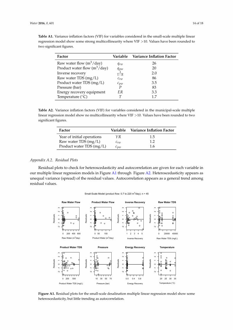
Variance inflation factors to check for multicollinearity (when VIF >10) are given for eachexplanatory variable in our multiple linear regression models in Table A1 through Table A2.

Water 2016, 8, 601 14 of 18

Table A1. Variance inflation factors (VIF) for variables considered in the small-scale multiple linearregression model show some strong multicollinearity where VIF >10. Values have been rounded totwo significant figures.

Factor Variable Variance Inflation Factor

Raw water flow (m3/day) qrw 26Product water flow (m3/day) qpw 20Inverse recovery 1

1−R 2.0Raw water TDS (mg/L) crw 86Product water TDS (mg/L) cpw 3.5Pressure (bar) P 83Energy recovery equipment ER 3.3Temperature (◦C) T 1.7

Table A2. Variance inflation factors (VIF) for variables considered in the municipal-scale multiplelinear regression model show no multicollinearity where VIF >10. Values have been rounded to twosignificant figures.

Factor Variable Variance Inflation Factor

Year of initial operations YR 1.5Raw water TDS (mg/L) crw 1.2Product water TDS (mg/L) cpw 1.6

Appendix A.2. Residual Plots

Residual plots to check for heteroscedasticity and autocorrelation are given for each variable inour multiple linear regression models in Figure A1 through Figure A2. Heteroscedasticity appears asunequal variance (spread) of the residual values. Autocorrelation appears as a general trend amongresidual values.

0 200 400 600

-2-1

01

23

Raw Water Flow

Raw Water (m3/day)

Residuals

0 50 150

-2-1

01

23

Product Water Flow

Product Water (m3/day)

Residuals

1 2 3 4 5

-2-1

01

23

Inverse Recovery

Inverse Recovery

Residuals

0 20000 40000

-2-1

01

23

Raw Water TDS

Raw Water TDS (mg/L)

Residuals

0 200 500

-2-1

01

23

Product Water TDS

Product Water TDS (mg/L)

Residuals

10 30 50 70

-2-1

01

23

Pressure

Pressure (bar)

Residuals

0.0 0.4 0.8

-2-1

01

23

Energy Recovery

Energy Recovery

Residuals

20 25 30 35

-2-1

01

23

Temperature

Temperature (°C)

Residuals

Small-Scale Model (product flow: 0.7 to 220 m3/day); n = 45

Figure A1. Residual plots for the small-scale desalination multiple linear regression model show someheteroscedasticity, but little trending as autocorrelation.

Water 2016, 8, 601 15 of 18

1990 2000 2010

-1.0

-0.5

0.0

0.5

1.0

Year

Year

Residuals

0 20000 40000-1.0

-0.5

0.0

0.5

1.0

Raw Water TDS

Raw Water TDS (mg/L)

Residuals

0 100 200 300 400 500

-1.0

-0.5

0.0

0.5

1.0

Product Water TDS

Product Water TDS (mg/L)

Residuals

Municipal-Scale Model (product flow: 2500 to 368,000 m3/day); n = 36

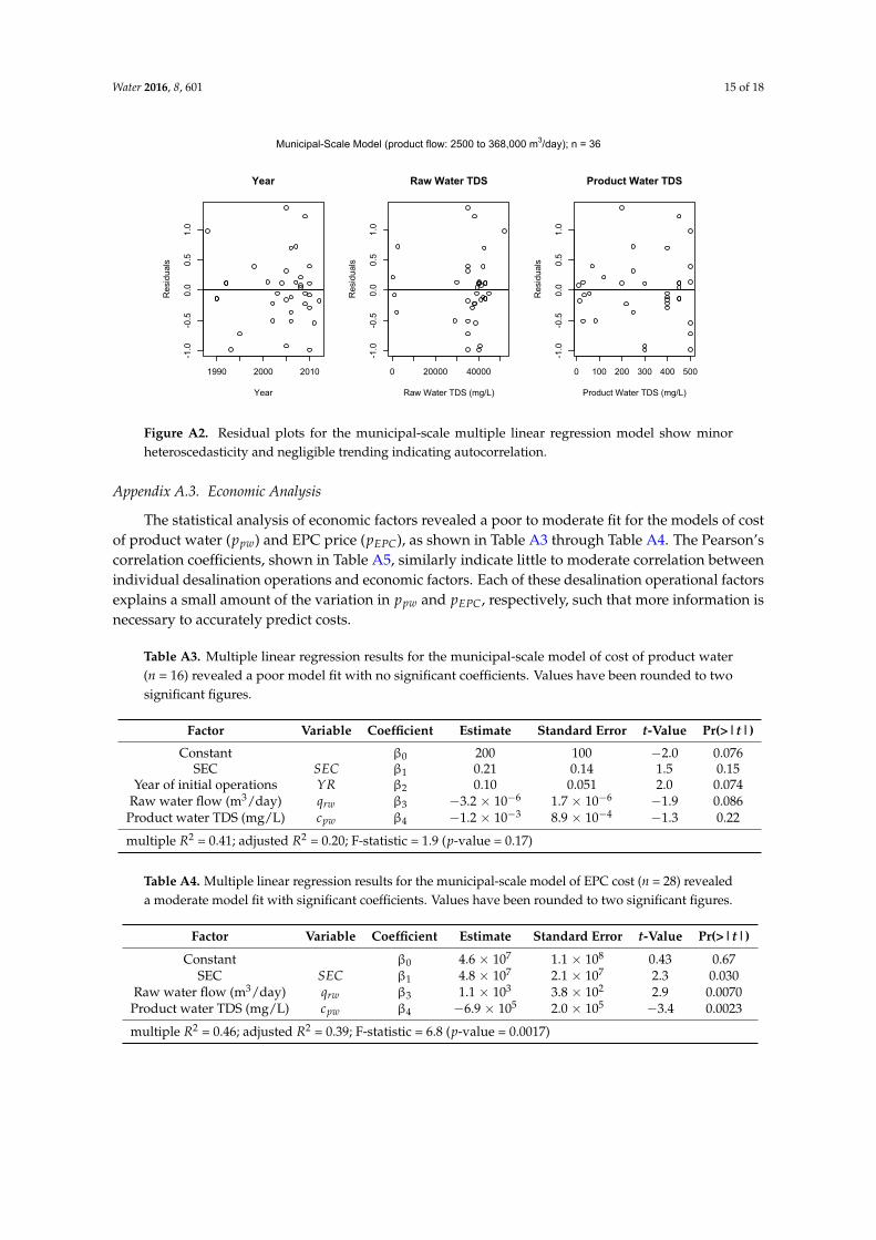
Figure A2. Residual plots for the municipal-scale multiple linear regression model show minorheteroscedasticity and negligible trending indicating autocorrelation.

Appendix A.3. Economic Analysis

The statistical analysis of economic factors revealed a poor to moderate fit for the models of costof product water (ppw) and EPC price (pEPC), as shown in Table A3 through Table A4. The Pearson’scorrelation coefficients, shown in Table A5, similarly indicate little to moderate correlation betweenindividual desalination operations and economic factors. Each of these desalination operational factorsexplains a small amount of the variation in ppw and pEPC, respectively, such that more information isnecessary to accurately predict costs.

Table A3. Multiple linear regression results for the municipal-scale model of cost of product water(n = 16) revealed a poor model fit with no significant coefficients. Values have been rounded to twosignificant figures.

Factor Variable Coefficient Estimate Standard Error t-Value Pr(>|t|)

Constant β0 200 100 −2.0 0.076SEC SEC β1 0.21 0.14 1.5 0.15

Year of initial operations YR β2 0.10 0.051 2.0 0.074Raw water flow (m3/day) qrw β3 −3.2 × 10−6 1.7 × 10−6 −1.9 0.086

Product water TDS (mg/L) cpw β4 −1.2 × 10−3 8.9 × 10−4 −1.3 0.22

multiple R2 = 0.41; adjusted R2 = 0.20; F-statistic = 1.9 (p-value = 0.17)

Table A4. Multiple linear regression results for the municipal-scale model of EPC cost (n = 28) revealeda moderate model fit with significant coefficients. Values have been rounded to two significant figures.

Factor Variable Coefficient Estimate Standard Error t-Value Pr(>|t|)

Constant β0 4.6 × 107 1.1 × 108 0.43 0.67SEC SEC β1 4.8 × 107 2.1 × 107 2.3 0.030

Raw water flow (m3/day) qrw β3 1.1 × 103 3.8 × 102 2.9 0.0070Product water TDS (mg/L) cpw β4 −6.9 × 105 2.0 × 105 −3.4 0.0023

multiple R2 = 0.46; adjusted R2 = 0.39; F-statistic = 6.8 (p-value = 0.0017)

Water 2016, 8, 601 16 of 18

Table A5. Pertinent Pearson’s correlation coefficients (ρ) for different municipal-scale desalinationfactors and economic considerations of cost of product water, ppw, and EPC price, pEPC, reveal little tomoderate correlation between factors. Values have been rounded to two significant figures.

Correlation ppw pEPC

SEC 0.20 −0.041crw 0.24 0.061cpw −0.38 −0.47

References

1. Grubert, E.A.; Stillwell, A.S.; Webber, M.E. Where does solar-aided seawater desalination make sense?A method for identifying sustainable sites. Desalination 2014, 339, 10–17.

2. Stillwell, A.S.; King, C.W.; Webber, M.E.; Duncan, I.J.; Hardberger, A. The Energy-Water Nexus in Texas.Ecol. Soc. 2011, 16, 2.

3. Sanders, K.T. Critical Review: Uncharted Waters? The Future of the Electricity-Water Nexus. Environ. Sci. Technol.2015, 49, 51–66.

4. Zhou, Y.; Tol, R.S.J. Evaluating the costs of desalination and water transport. Water Resour. Res. 2005, 41, 1–10.5. Reddy, K.V.; Ghaffour, N. Overview of the cost of desalinated water and costing methodologies. Desalination

2007, 205, 340–353.6. Einav, R.; Harussi, K.; Perry, D. The footprint of desalination processes on the environment. Desalination

2002, 152, 141–154.7. Lattemann, S.; Höpner, T. Environmental impact and impact assessment of seawater desalination. Desalination

2008, 220, 1–15.8. Younos, T. Environmental Issues in Desalination. J. Contemp. Water Res. Educ. 2005, 132, 11–18.9. Zander, A.K.; Elimelech, M.; Furukawa, D.H.; Gleick, P.; Herd, K.; Jones, K.L.; Rolchigo, P.; Sethi, S.; Tonner, J.;

Vaux, H.J.; et al. Desalination: A National Perspective; Technical Report; Committee on Advancing DesalinationTechnology, National Research Council: Washington, DC, USA, 2008.

10. Buffle, M.O. Water, Water, Everywhere, Many a Drop to Drink. Available online: http://www.robecosam.com/en/sustainability-insights/library/foresight/2013/Water-water-everywhere-many-a-drop-to-drink.jsp(accessed on 7 January 2013).

11. Cooley, H.; Gleick, P.H.; Wolff, P. Desalination, With a Grain of Salt: A California Perspective; Technical Report;Pacific Institute: Oakland, CA, USA, 2006.

12. Dow Water & Process Solutions. ROSA System Design Software. Available online: http://www.dow.com/en-us/water-and-process-solutions/resources/design-software/rosa-software (accessed on18 November 2016).

13. Hydranautics. IMSDesign: Integrated Membranes Solution Design. Available online: http://www.hydranauticsprojections.net/imsd/downloads/ (accessed on 18 November 2016).

14. Global Water Intelligence. DesalData.com. Available online: http://desaldata.com (accessed on 12 July 2016).15. International Desalination Association. Desalination By the Numbers. Available online: http://idadesal.

org/desalination-101/desalination-by-the-numbers/ (accessed on 30 June 2015).16. Semiat, R. Energy Issues in Desalination Processes. Environ. Sci. Technol. 2008, 42, 8193–8201.17. Huehmer, R.; Wang, F. Energy in Desalination: Comparison of Energy Requirements for Developing

Desalination Techniques, 2009. In Proceedings of the AWWA Membrane Technology Conference, Memphis,TN, USA, 15–18 March 2009.

18. Elimelech, M.; Phillip, W.A. The Future of Seawater Desalination: Energy, Technology, and the Environment.Science 2011, 333, 712–717.

19. Fritzmann, C.; Löwenberg, J.; Wintgens, T.; Melin, T. State-of-the-art of reverse osmosis desalination. Desalination2007, 216, 1–76.

20. Darwish, M.A.; Al Asfour, F.; Al-Najem, N. Energy consumption in equivalent work by different desaltingmethods: Case study for Kuwait. Desalination 2002, 152, 83–92.

21. McGinnis, R.L.; Elimelech, M. Energy requirements of ammonia-carbon dioxide forward osmosis desalination.Desalination 2007, 207, 370–382.

Water 2016, 8, 601 17 of 18

22. Veza, J.M.; Peñate, B.; Castellano, F. Electrodialysis desalination designed for off-grid wind energy. Desalination2004, 160, 211–221.

23. Al-Karaghouli, A.; Kazmerski, L.L. Energy consumption and water production cost of conventional andrenewable-energy-powered desalination processes. Renew. Sustain. Energy Rev. 2013, 24, 343–356.

24. McGovern, R.K.; Lienhard V, J.H. On the potential of forward osmosis to energetically outperform reverseosmosis desalination. J. Membr. Sci. 2014, 469, 245–250.

25. Miller, S.; Shemer, H.; Semiat, R. Energy and environmental issues in desalination. Desalination 2015, 366, 2–8.26. Schallenberg-Rodríguez, J.; Veza, J.M.; Blanco-Marigorta, A. Energy efficiency and desalination in the

Canary Islands. Renew. Sustain. Energy Rev. 2014, 40, 741–748.27. Carta, J.A.; González, J.; Cabrera, P.; Subiela, V.J. Preliminary experimental analysis of a small-scale prototype

SWRO desalination plant, designed for continuous adjustment of its energy consumption to the widelyvarying power generated by a stand-alone wind turbine. Appl. Energy 2015, 137, 222–239.

28. Ghalavand, Y.; Hatamipour, M.S.; Rahimi, A. A review on energy consumption of desalination processes.Desalin. Water Treat. 2015, 54, 1526–1541.

29. Gordon, J.M.; Chua, H.T. Thermodynamic perspective for the specific energy consumption of seawaterdesalination. Desalination 2016, 386, 13–18.

30. Lin, S.; Elimelech, M. Staged reverse osmosis operation: Configurations, energy efficiency, and applicationpotential. Desalination 2015, 366, 9–14.

31. Mazlan, N.M.; Peshev, D.; Livingston, A.G. Energy consumption for desalination—A comparison of forwardosmosis with reverse osmosis, and the potential for perfect membranes. Desalination 2016, 377, 138–151.

32. Shrivastava, A.; Rosenberg, S.; Peery, M. Energy efficiency breakdown of reverse osmosis and its implicationson future innovation roadmap for desalination. Desalination 2015, 368, 181–192.

33. Feinberg, B.J.; Ramon, G.Z.; Hoek, E.M.V. Thermodynamic Analysis of Osmotic Energy Recovery at a ReverseOsmosis Desalination Plant. Environ. Sci. Technol. 2013, 47, 2982–2989.

34. Spiegler, K.S.; El-Sayed, Y.M. The energetics of desalination processes. Desalination 2001, 134, 109–128.35. Avlonitis, S.A.; Avlonitis, D.A.; Panagiotidis, T. Experimental study in the specific energy consumption for

brackish water desalination by reverse osmosis. Int. J. Energy Res. 2012, 36, 36–45.36. Wilf, M.; Klinko, K. Optimization of seawater RO systems design. Desalination 2001, 138, 299–306.37. Wilf, M.; Klinko, K. Performance of commercial seawater membranes. Desalination 1994, 96, 465–478.38. Atab, M.S.; Smallbone, A.J.; Roskilly, A.P. An operational and economic study of a reverse osmosis desalination

system for potable water and land irrigation. Desalination 2016, 397, 174–184.39. Choi, J.S.; Kim, J.T. Modeling of full-scale reverse osmosis desalination system: Influence of operational

parameters. J. Ind. Eng. Chem. 2015, 21, 261–268.40. Zhu, A.; Christofides, P.D.; Cohen, Y. Effect of Thermodynamic Restriction on Energy Cost Optimization of

RO Membrane Water Desalination. Ind. Eng. Chem. Res. 2009, 48, 6010–6021.41. Avlonitis, S.A.; Kouroumbas, K.; Vlachakis, N. Energy consumption and membrane replacement cost for

seawater RO desalination plants. Desalination 2003, 157, 151–158.42. Peñate, B.; García-Rodríguez, L. Energy optimisation of existing SWRO (seawater reverse osmosis) plants

with ERT (energy recovery turbines): Technical and thermoeconomic assessment. Energy 2011, 36, 613–626.43. Ruiz-García, A.; Nuez, I. Long-term performance decline in a brackish water reverse osmosis desalination

plant. Predictive model for water permeability coefficient. Desalination 2016, 397, 101–107.44. Li, M. Reducing specific energy consumption in Reverse Osmosis (RO) water desalination: An analysis from

first principles. Desalination 2011, 276, 128–135.45. Werber, J.R.; Osuji, C.O.; Elimelech, M. Materials for next-generation desalination and water purification

membranes. Nat. Rev. Mater. 2016, 1, 1–15.46. Werber, J.R.; Deshmukh, A.; Elimelech, M. The Critical Need for Increased Selectivity, Not Increased Water

Permeability, for Desalination Membranes. Environ. Sci. Technol. Lett. 2016, 3, 112–120.47. Werber, J.R.; Deshmukh, A.; Elimelech, M. Can batch or semi-batch processes save energy in reverse-osmosis

desalination? Desalination 2017, 402, 109–122.48. Elhassadi, A. Horizons and future of water desalination in Libya. Desalination 2008, 220, 115–122.49. Greenlee, L.F.; Lawler, D.F.; Freeman, B.D.; Marrot, B.; Moulin, P. Reverse osmosis desalination:

Water sources, technology, and today’s challenges. Water Res. 2009, 43, 2317–2348.

Water 2016, 8, 601 18 of 18

50. Ghaffour, N.; Missimer, T.M.; Amy, G.L. Technical review and evaluation of the economics of water desalination:Current and future challenges for a better water supply sustainability. Desalination 2013, 309, 197–207.

51. Gujarati, D.N. Basic Econometrics, 4th ed.; McGraw-Hill Companies: New York, NY, USA, 2003.52. Busch, M.; Mickols, W.E. Reducing energy consumption in seawater desalination. Desalination 2004, 165, 299–312.53. Jacangelo, J.G.; Oppenheimer, J.A.; Subramani, A.; Badruzzaman, M. Desalination Strategies for Energy

Optimization and Renewable Energy Use. IDA J. 2012, 4, 28–33.54. Ma, Q.; Lu, H. Wind energy technologies integrated with desalination systems: Review and state-of-the-art.

Desalination 2011, 277, 274–280.55. Macedonio, F.; Curcio, E.; Drioli, E. Integrated membrane systems for seawater desalination: Energetic and

exergetic analysis, economic evaluation, experimental study. Desalination 2007, 203, 260–276.56. Mohamed, E.S.; Papadakis, G. Design, simulation and economic analysis of a stand-alone reverse osmosis

desalination unit powered by wind turbines and photovoltaics. Desalination 2004, 164, 87–97.57. Mohsen, M.S.; Jaber, J.O. A photovoltaic-powered system for water desalination. Desalination 2001, 138, 129–136.58. Park, G.L.; Schäfer, A.I.; Richards, B.S. The effect of intermittent operation on a wind-powered membrane

system for brackish water desalination. Water Sci. Technol. 2012, 65, 867–874.59. Swift, A.; Rainwater, K.; Chapman, J.; Noll, D.; Jackson, A.; Ewing, B.; Song, L.; Ganesan, G.; Marshall, R.;

Doon, V.; et al. Wind Power and Water Desalination Technology Integration; Technical Report Desalination andWater Purification Research and Development Program Report No. 146; U.S. Department of the Interior,Bureau of Reclamation: Texas Tech University, Lubbock, TX, USA, 2009.

60. Takabatake, H.; Noto, K.; Uemura, T.; Ueda, S. More than 30% energy saving seawater desalination systemby combining with sewage reclamation. Desalin. Water Treat. 2013, 51, 733–741.

61. Weiner, D.; Fisher, D.; Moses, E.J.; Katz, B.; Meron, G. Operation experience of a solar- and wind-powereddesalination demonstration plant. Desalination 2001, 137, 7–13.

62. Tonidandel, S.; LeBreton, J.M. Relative Importance Analysis: A Useful Supplement to Regression Analysis.J. Bus. Psychol. 2011, 26, 1–9.

63. Tonidandel, S.; LeBreton, J.M. Relative Importance Analysis: Programs for Calculating Relative Weights inMultiple, Multivariate, and Logistic Regression. Available online: http://relativeimportance.davidson.edu/multipleregression.html (accessed on 18 November 2016).

64. McCuen, R.H. Modeling Hydrologic Change: Statistical Methods, 1st ed.; Taylor & Francis Group: Boca Raton,FL, USA, 2003.

65. Global Water Intelligence. SWRO Cost Estimator. Available online: http://desaldata.com/cost_estimator(accessed on 30 June 2016).

66. Gorman, S. California Drought Renews Thirst for Desalination Plants. Available online: http://www.reuters.com/article/2015/04/15/us-usa-desalination-california-idUSKBN0N601V20150415 (accessed on14 April 2015).

67. Carlsbad Desalination Project. Energy Minimization and Greenhouse Gas Reduction Plan; Technical Report;Poseidon Resources: Carlsbad, CA, USA, 2008.

68. Stokes, J.R.; Horvath, A. Energy and Air Emission Effects of Water Supply. Environ. Sci. Technol. 2009, 43,2680–2687.

69. Clayton, M.E.; Stillwell, A.S.; Webber, M.E. Implementation of Brackish Groundwater Desalination UsingWind-Generated Electricity: A Case Study of the Energy-Water Nexus in Texas. Sustainability 2014, 6, 758–778.

70. Gold, G.M.; Webber, M.E. The Energy-Water Nexus: An Analysis and Comparison of Various ConfigurationsIntegrating Desalination with Renewable Power. Resources 2015, 4, 227–276.

71. Kjellsson, J.B.; Webber, M.E. The Energy-Water Nexus: Spatially-Resolved Analysis of the Potential forDesalinating Brackish Groundwater by Use of Solar Energy. Resources 2015, 4, 476–489.

72. Voutchkov, N. Power Plant Co-Location Reduces Desalination Costs, Environmental Impacts.Available online: http://www.waterworld.com/articles/iww/print/volume-8/issue-1/columns/product-focus/power-plant-co-location-reduces-desalination-costs-environmental-impacts.html (accessed on18 November 2016).

© 2016 by the authors; licensee MDPI, Basel, Switzerland. This article is an open accessarticle distributed under the terms and conditions of the Creative Commons Attribution(CC-BY) license (http://creativecommons.org/licenses/by/4.0/).