University of Pennsylvania University of Pennsylvania

ScholarlyCommons ScholarlyCommons

Operations, Information and Decisions Papers Wharton Faculty Research

9-2006

Revenue Management Through Dynamic Cross Selling in E-Revenue Management Through Dynamic Cross Selling in E-

Commerce Retailing Commerce Retailing

Serguei Netessine University of Pennsylvania

Sergei Savin

Wenqiang Xiao

Follow this and additional works at: https://repository.upenn.edu/oid_papers

Part of the Marketing Commons, Sales and Merchandising Commons, and the Strategic Management

Policy Commons

Recommended Citation Recommended Citation Netessine, S., Savin, S., & Xiao, W. (2006). Revenue Management Through Dynamic Cross Selling in E-Commerce Retailing. Operations Research, 54 (5), 893-913. http://dx.doi.org/10.1287/opre.1060.0296

This paper is posted at ScholarlyCommons. https://repository.upenn.edu/oid_papers/123 For more information, please contact repository@pobox.upenn.edu.

Revenue Management Through Dynamic Cross Selling in E-Commerce Retailing Revenue Management Through Dynamic Cross Selling in E-Commerce Retailing

Abstract Abstract We consider the problem of dynamically cross-selling products (e.g., books) or services (e.g., travel reservations) in the e-commerce setting. In particular, we look at a company that faces a stream of stochastic customer arrivals and may offer each customer a choice between the requested product and a package containing the requested product as well as another product, what we call a “packaging complement.” Given consumer preferences and product inventories, we analyze two issues: (1) how to select packaging complements, and (2) how to price product packages to maximize profits.

We formulate the cross-selling problem as a stochastic dynamic program blended with combinatorial optimization. We demonstrate the state-dependent and dynamic nature of the optimal package selection problem and derive the structural properties of the dynamic pricing problem. In particular, we focus on two practical business settings: with (the Emergency Replenishment Model) and without (the Lost-Sales Model) the possibility of inventory replenishment in the case of a product stockout. For the Emergency Replenishment Model, we establish that the problem is separable in the initial inventory of all products, and hence the dimensionality of the dynamic program can be significantly reduced. For both models, we suggest several packaging/pricing heuristics and test their effectiveness numerically.

Keywords Keywords dynamic programming/optimal control, models, marketing, pricing ; buyer behavior

Disciplines Disciplines Marketing | Sales and Merchandising | Strategic Management Policy

This journal article is available at ScholarlyCommons: https://repository.upenn.edu/oid_papers/123

Revenue Management through Dynamic Cross-Selling in

E-commerce Retailing∗

Serguei Netessine†

The Wharton School

University of Pennsylvania

Sergei Savin‡, Wenqiang Xiao§,Graduate School of Business

Columbia University

April 2004, Revised November 2004

Abstract

We consider the problem of dynamically cross-selling products (e.g., books) or services (e.g., travel

reservations) in the e-commerce setting. In particular, we look at a company that faces a stream of stochastic

customer arrivals and may offer each customer a choice between the requested product and a package

containing the requested product as well as another product, “packaging complement”. Given consumer

preferences and product inventories, two issues are analyzed: (1) how to select packaging complements and

(2) how to price product packages to maximize profits.

We formulate the cross-selling problem as a stochastic dynamic program blended with combinatorial

optimization. We demonstrate the state-dependent and dynamic nature of the optimal package selection

problem and derive structural properties of the dynamic pricing problem. In particular, we focus on

two practical business settings: with (the Emergency Replenishment model) and without (the Lost Sales

model) the possibility of inventory replenishment in the case of a product stock-out. For the Emergency

Replenishment model, we establish that the problem is separable in the initial inventory of all products and

hence the dimensionality of the dynamic program can be significantly reduced. For both models several

packaging/pricing heuristics are suggested and their effectiveness is tested numerically.

∗We are grateful to the Departmental Editor, Associate Editor and two anonymous referees for suggestions that helped improvethe paper.

†Email: netessine@wharton.upenn.edu‡Email: svs30@columbia.edu§Email: wx2004@columbia.edu

1

1 Introduction

The development of the Internet has provided significant opportunities for new business models and retailing

practices partly because massive amounts of click-stream data have become available to companies and the

implementation of many decisions in real time has become virtually costless. For example, Internet companies

can change prices dynamically and observe consumer response. Additionally, promotional decisions (discounts,

rebates, etc.) can be made dynamically. These new opportunities pose challenges to researchers in various

areas of business and economics: decisions that were previously made in a static environment must now take

into account the dynamic potential of Internet retailing.

One practice that has recently been widely adopted on the Internet is dynamic cross-selling. For example,

an attempt to buy most books on Amazon.com will generate a suggestion to buy a package of two or more

books1. We screened the top 100 books from Amazon.com’s best-selling list for September 17, 2003 to identify

configurations of cross-selling suggestions (see Table 1 for results). As is evident from this sample, only a

small fraction of books (7%) was not offered in a package with any other book. Further evidence from a

recent survey by The E-tailing Group Inc. [11] suggests that 62% of the top 100 Internet retailers utilize

various forms of cross-selling. Other prominent examples of dynamic cross-selling are found among travel-

related Internet companies that term this practice “dynamic packaging” [2]. All these observations underscore

the importance of understanding the trade-offs involved in dynamic cross-selling decisions and the need to

quantify the benefits from making these decisions optimally.

Cross-selling is widely acknowledged as an important part of Customer Relationship Management (CRM).

However, the implementation of dynamic cross-selling on the Internet poses several challenges. For example,

the choice of products to cross-sell must be made by the “software” on the basis of information about product

inventories and customer preferences rather than by a sales associate who can ask additional questions. That

is, dynamic cross-selling must be performed in response to every customer’s purchase attempt rather than

using pre-set static rules. To see challenges associated with implementing dynamic cross-selling, note that

cross-selling packages are often offered at a discount so that a package of products would generate lower profit

margins. Hence, if inventory for one of the products in the package is low, it might be more profitable for

a company to sell products individually because there is a good chance that the product will be sold later

at full price2. As a result, the current inventory situation must be incorporated into cross-selling decisions.

The obvious complexity of the decisions involved in dynamic cross-selling on the Internet has resulted in the

need for specialized software packages. Some examples of companies offering such software are Netperceptions

(focusing on physical goods) and PROS (focusing on travel-related services). At the same time, academic

research on dynamic cross-selling is essentially non-existent. The goal of this paper is to fill this void by

providing a deeper understanding of the dynamic cross-selling problem by building the framework for its

analysis, outlining the trade-offs involved, obtaining structural results and deriving efficient solution methods.

We begin by proposing a novel modeling framework for the dynamic cross-selling problem in which com-

1At the time of this writing, Amazon.com did not offer discounts on book packages.2In this respect, the situation with selling a product as part of a package at a discount now or selling products individually

later is similar to the standard yield management problem that is common for airlines.

2

binatorial optimization (package selection) is blended with the stochastic dynamic program (package pricing)

over a finite time horizon. The time horizon is subdivided into smaller decision epochs corresponding to pack-

aging and pricing decisions that are made more often than inventory replenishments. Customer arrivals are

modeled as a stochastic, discrete-time process. Each customer attempting to buy one product (which we call

first-choice) is offered a package of this product with another one (which we call packaging complement) and

can (with some probability that depends on the price of the package) choose to buy a package. We demon-

strate the dynamic and state-dependent nature of the optimal package selection problem and concentrate

on obtaining structural properties for the dynamic pricing problem. The combinatorial problem of optimal

package selection is later re-visited using heuristic approaches.

Two important business settings are further analyzed. In the first setting, the firm has an opportunity

to procure an out-of-stock product at an extra cost (the Emergency Replenishment model, hereafter the ER

model). For this model we show that, under any static packaging scheme, the value function is separable in

the initial inventory levels of all products and hence the dimensionality of the dynamic program (hereafter, the

DP) can be greatly reduced. We refer to this result as a decomposition property. We also show that the value

function is non-decreasing concave in the initial inventory levels of all products and the optimal price of the

package is a non-increasing function of time and of the inventory of the packaging complement. Interestingly,

the optimal package price in this case is independent of the inventory of the first-choice product. In the

second setting (the Lost Sales model, hereafter the LS model), product inventory cannot be replenished and

the customer’s request is simply denied if the product is out of stock. We show (through counterexamples)

that few of the properties of the ER model continue to hold in this case. Most importantly, the value function

is no longer separable in product inventories: in fact, for the two-product case, we show that the value function

is supermodular. Moreover, the value function is generally not concave in product inventories. Under the

arbitrary static product packaging rule, upper and a lower bounds for the value function are derived and used

to identify settings in which the revenue function is relatively insensitive to the choice of a particular static

packaging scheme. Finally, for both the ER and the LS models we suggest several heuristic solution approaches

and test them numerically. We comment on the comparative advantages and robustness of different heuristics.

To summarize, this paper makes three main contributions. First, we identify dynamic cross-selling as

an application of revenue management/dynamic pricing but one that involves an additional combinatorial

optimization to select the packaging complement. We also propose a novel modeling framework to analyze the

cross-selling (packaging/pricing) problem. We derive the structural properties of the dynamic pricing problem

under any static packaging scheme, most notably the decomposition property of the objective function in the

ER model. Finally, we explore the structural properties of these models to obtain efficient dynamic packaging

and pricing heuristics. Two of the proposed heuristics, the so-called “two-stage” approach and the “depletion

rate” heuristic, are shown numerically to have a near-optimal performance over a wide range of problem

parameters. The rest of the paper is organized as follows. In the remainder of this section we survey related

literature. In Section 2 we state modeling assumptions and formulate the problem. Sections 3 and 4 contain

analysis of the ER and LS models, respectively. Section 5 concludes with a discussion of our results.

3

1.1 Related literature

In recent years the practice of cross-selling and the related practice of up-selling are receiving more and

more coverage in trade publications (see, for example, Feldman [14], Peters [27]), while academic research

on cross-selling is very sparse: the works of Nash and Sterna-Karwat [24] describing the application of DEA

methodology to cross-sell financial services and of Kamakura et al. [19] utilizing customer databases to identify

opportunities for cross-selling are the only papers addressing this issue. To the best of our knowledge, there

are no papers that either model or analyze dynamic cross-selling that involves the dynamic pricing of packages

and dynamic package selection.

The dynamic package pricing decision is closely related to the large stream of operations literature on

dynamic pricing and revenue management (see McGill and van Ryzin [21] and Bitran and Caldentey [8] for

surveys). In another recent survey, Elmaghraby and Keskinocak [9] provide a thorough discussion of the need

to incorporate customized pricing considerations (of which cross-selling is one example) into dynamic pricing

models; they cite many applications and notice that there are no papers in the extant literature addressing

this problem. Other publications in this stream typically consider the dynamic pricing of a single product and

hence do not address cross-selling issues (see, for example, Gallego and van Ryzin [16] and Aviv and Pazgal

[6]). Monahan et al. [23] study the problem of pricing a single product over multiple time periods after a

single inventory decision. Their setting is similar to ours in that the product is sold over multiple periods

without further replenishments. However, they utilize a specific form of demand function: random shock is

multiplicative and price dependence is iso-elastic, which allows them to find optimal prices and inventory in a

closed form. An alternative setting is the one in which demand from several types of customers can be satisfied

with the same capacity (see Maglaras and Meissner [20]). In our paper, demand from a customer may involve

several types of inventory simultaneously. In this respect, we believe that the papers most relevant to our

work are those analyzing the dynamic revenue management of multiple products, a rather sparsely populated

area of literature (see Gallego and van Ryzin [17], Zhang and Cooper [34]).

On the Internet, the selection of the packaging complement can be based both on the customer information

acquired during previous transactions and/or on the customer profile. To process the significant amounts

of data necessary for making decisions, companies utilize data mining techniques (see Padmanabhan and

Tuzhilin [26] for a survey of relevant methodologies). This approach is generally termed “personalization” (see

Adomavicius and Tuzhilin [5]). Papers dealing with personalization techniques typically focus on generating a

recommendation that ensures the best match between the customer and the product regardless of the potential

impact on the firm’s profitability. On the contrary, we assume that the company uses data mining to generate

the probability distribution over customers’ purchase preferences, which in turn is used to cross-sell products

to maximize the firm’s profit. Hence, it is quite possible that the package offered to the customer is not the

best possible match from the personalization perspective.

A practice related to cross-selling is product bundling, which also attempts to sell a package consisting

of several products rather that selling just a single product. However, bundling decisions (involving what to

bundle and how to price bundles) are static and made before customer arrival; this differs from cross-selling,

which is done only after a customer declares a desire to buy something. Nevertheless, dynamic cross-selling

can be loosely interpreted as dynamic bundling, so we briefly review the related literature. Economists were

4

the first to analyze the concept of bundling (see Stigler [31]). The cornerstone for many subsequent papers

on product bundling was the seminal work of Adams and Yellen [4], who formulated a model with a firm

selling two products as well as a bundle of these two products and demonstrated the benefits arising from

bundling. In the operations literature Hanson and Martin [18] were, perhaps, the first to address the problem

of optimally pricing bundles of products using a mathematical programming approach in a static model. Ernst

and Kouvelis [10] study the issue of how much of each individual product as well as how many bundles to stock

while pricing and bundling decisions are exogenous to the model. There is a wealth of marketing literature

considering bundling with a particular emphasis on static pricing. Rao [29] and Stremersch and Tellis [32]

review this stream. In addition, an extensive collection of papers on this topic can be found in Fuerderer et

al. [15]. In all of these papers, a commitment to sell bundles is made prior to demand arrival and thereafter

prices/bundles cannot be altered. Hence, the underlying models are static rather than dynamic. We are not

aware of any papers analyzing dynamic product bundling.

2 Modeling dynamic cross-selling decisions

We consider an environment in which an online retail company is selling a group of m products. We assume

that all products in the group target similar market segments and can therefore potentially be cross-sold

with each other (see examples in the introduction). We further assume that the planning horizon is finite

(representing the time between two inventory replenishments) and is separated into N decision epochs. At the

beginning of each decision epoch the company observes the inventory of each product and makes cross-selling

(packaging and pricing) decisions. In the online environment packaging and pricing decisions can be made

as frequently as necessary, so that the length of each decision epoch can be made short compared to typical

customer interarrival time. Consequently, we assume that within each epoch there is at most one customer

arrival. We denote by λi, i = 1, ...,m, the probability that during any decision epoch class i customer arrives

and requests one unit of i-th product (Pmi=1 λi < 1 to reflect the possibility that there is no customer arrival

in a particular decision epoch). Alternatively, one can also define the probability that arriving customers do

not buy a product, but the problem can be easily re-formulated to focus on customers that are willing to

make a purchase.3

Upon requesting product i at a fixed price4 pi, a class i customer receives an offer of a “product i-product

j” package (for some j) at a price pij . We assume that only one package of only two products is offered to the

customer, which is consistent with the practice of some companies. Our experiment with Amazon.com’s best-

seller list (see Table 1) shows that at most one packaging complement is used for each available product. We

assume that class i customers have a reservation price for “i-j” package distributed according to a cdf Fij (·)

3The implicit assumption here is that the probability of purchasing a product is time-invariant while in practice this probabilitymay be affected by the firm’s decisions. E.g., intensive cross-selling of product j may result in fewer customers buying this productin the future.

4In our analysis, we consider individual product price to be fixed but package price to be dynamic. This approach is oftenjustified in practice, since some Internet retailers try to avoid dynamically changing prices of individual products for fear ofantagonizing customers (see the example of Amazon.com’s experience [1]). Alternatively, our analysis can complement thetraditional single-product revenue management literature which studies the effects of dynamically changing prices for individualproducts (see McGill and van Ryzin [21] for a thorough survey).

5

with non-negative support. Consequently, a class i customer buys the package at a price pij with probability

F ij (pij) = 1 − Fij (pij) , and buys only product i at price pi with probability Fij (pij)5. We assume thatF̄ij(x)(x − y) is a unimodal function of x for any nonnegative constant y. This assumption holds for a wideclass of distribution functions and is also a standard assumption often made in the pricing literature, see Ziya

et al. [37] for discussion and references.

The issue of estimating Fij (pij) is an important one that merits a separate study. For our purposes,

we simply assume that Fij (pij) is obtained by analyzing customer shopping behavior using data mining

techniques. Two examples of approaches that can potentially be utilized in this case are found in Moe and

Fader [22] and Bertsimas et al. [7]. Since we do not assume any particular functional form for these probability

functions, any approach can be accommodated by our model. Note also that we classify customers based on

the product they request, while in practice a company may have additional customer information that would

allow for fine-tuning probability estimation further. In the extreme, each arriving customer could be treated

as a separate class. Our model can be extended to incorporate such a possibility (e.g., let k be the customer

index with each customer having a unique k so that λi =Pk λ

ki where λ

ki represents customer k arriving to

request book i) but at a cost of additional notation that would make exposition less tractable. To support

our approach, there is some evidence that for a cross-selling recommendation, the first-choice product is more

relevant than the customer profile ([3]).

In each decision epoch a company needs to decide, for each product i, which product j should be “packaged”

with it and what price should be established for such a package. Suppose that at the beginning of the n-th

decision epoch (n = 1, ..., N) the inventory levels of products are given by vector I = (I1, ..., Im) and let Vn (I)

be the optimal expected revenue accrued from that moment until the end of the planning horizon. Define

ei, i = 1, ...,m as an m-dimensional vector whose components are (ei)k = 1 if k = i and 0 otherwise. We

are interested in selecting a sequence of packaging and pricing decisions in order to maximize V1 (I) . The

functional form of the Bellman equation for Vn (I) depends on actual inventory levels. If there is at least one

unit of inventory for each product (Ii ≥ 1 for all i = 1, ...,m), the Bellman equation can be expressed as

Vn (I) =mXi=1

λimaxj 6=i

µmaxpij

¡Fij (pij) (pi + Vn+1 (I− ei)) + F ij (pij) (pij + Vn+1 (I− ei − ej))

¢¶

+

Ã1−

mXi=1

λi

!Vn+1 (I) . (1)

At the heart of the recursion (1) are two maximization operators reflecting the dynamic packaging and pricing

decisions. The “outer” maximization selects the “best” product j to be packaged with product i in the case

of a class i customer arrival, while the “inner” maximization selects the “best” price for each “i-j” package.

Without loss of generality, we assume that the inventory left in stock at the end of the planning horizon has

no salvage value and supplement (1) by the “end-of-horizon” condition VN+1 (I) = 0.

5A more general way to model this problem is to allow the consumer to choose simultaneously among products i, j and apackage ij. In this case the probability of selecting each of these options might depend on pi, pj and pij . However, our approach isplausible when product j has low value without product i (e.g., hotel reservation without air ticket) and it also matches practicallyobserved applications of cross-selling relatively well.

6

Clearly, the dynamic packaging problem is quite complex since it involves solving a large-scale combinato-

rial optimization superimposed on the stochastic DP. In fact, there are very few papers that successfully derive

structural results for such problems. To illustrate the complexity of this problem, we demonstrate that in the

settings in which the number of products is three or more, the choice of the best packaging complement is

non-trivial. In particular, the optimal packaging decisions may be state-dependent as well as dynamic. Figure

1 illustrates an example of the optimal package selection in the three-product case for the following problem

parameters: F ij(pij) = ((pi + pj − pij) /pj)β defined over [pi, pi + pj ], i, j = 1, 2, 3, with N = 10,β = 1,

p1 = p3 = 1, p2 = 1.5, and λ1 = λ2 = λ3 = 0.3. This form of the reservation function is reasonable because

F ij (pi) = 1 and F ij (pi + pj) = 0. Figure 1a shows how the optimal packaging at the beginning of the planning

horizon (n = 1) changes with the inventory of product 1: the packaging complement of product 2 oscillates

between products 1 and 3 in a rather unusual fashion. Such “non-monotone” behavior hints at a particularly

complex structural form of the optimal value function even for a relatively simple three-product case. Figure

1b illustrates the dynamic nature of the optimal packaging for the same state of the system: in this example,

the shrinking of the remaining time horizon forces product 1 to change its packaging complement from product

3 to product 2.

As the above example demonstrates, packaging decisions for more than two products are quite complex.

This interaction between dynamic packaging and pricing significantly complicates the analysis of the general

DP formulation. Below we begin our analysis by separating packaging and pricing decisions and focusing

on pricing first by assuming that packaging is static so that the packaging complement for each product is

fixed and does not change with the state of the product inventory or with time. This policy may be used by

a company intentionally to ensure that the packaging complement closely matches the first-choice product.

For example, the packaging complement can be assigned according to the closest match based on a purchase

history and/or on customer profile (of course, the packaging decision becomes trivial with only two products).

Thereafter we propose several (heuristic) ways to solve the dynamic packaging problem and will test them

numerically.

As mentioned above, the DP recursion (1) is applicable as long as there is at least one unit of inventory

left for each product. Hence, when the company runs out of inventory for one or more products, (1) needs to

be adjusted. Below we consider two alternative policies describing the company’s response to the request for

a product with zero inventory level. The first alternative, designated as the Emergency Replenishment model

(hereafter, ER), allows the company to procure a “missing” item i at an additional cost bi (to ensure that it

is always profitable to use ER in the case of a stockout we assume that bi ≤ pi). In Section 3 we prove thedecomposition property of the optimal value function for the ER model under any static packaging scheme,

enabling an efficient solution method for the multiproduct ER model. Under the second alternative, which we

call the Lost Sales model (hereafter, LS), the customer request is simply rejected. The LS model (analyzed in

Section 4) lacks such a decomposition property. Consequently, as the number of products grows, this model

becomes increasingly difficult to solve. For both models we propose heuristic approaches and analyze their

performance.

7

3 The Emergency Replenishment model

Under the ER model, the company has an opportunity to procure additional product inventory at an extra

cost. This assumption may be appropriate in settings with many physical products sold over the Internet.

For example, in case the retailer stocks out, products could be drop-shipped from the wholesaler directly to

the customers (i.e., the order is passed on to the wholesaler/distributor who performs the fulfillment at an

extra cost, see Netessine and Rudi [25] for details on drop-shipping arrangements and practical examples). In

this case, bi may represent the drop-shipping mark-up and/or additional shipping costs. Alternatively, the

retailer may re-order the missing item from the wholesaler and, once it arrives, utilize a faster delivery mode

to compensate for the delay (e.g., use next-day instead of the regular shipping service). In this situation, bi

may represent the extra transportation cost.

It is convenient to introduce sets of indices An to denote products that have at least one unit of inventory

at the beginning of the n-th decision epoch. Under the ER model the appropriate generalization of (1) is

given by

Vn (I) =Xi∈An

λimax (Hni , J

ni ) +

Xi/∈An

λimax¡Hni , J

ni

¢+

Ã1−

mXi=1

λi

!Vn+1 (I) , (2)

with

Hni = max

j 6=i, j∈An

µmaxpij

¡Fij (pij) (pi + Vn+1 (I− ei)) + F ij (pij) (pij + Vn+1 (I− ei − ej))

¢¶, (3)

Jni = maxj 6=i, j /∈An

µmaxpij

¡Fij (pij) (pi + Vn+1 (I− ei)) + F ij (pij) (pij − bj + Vn+1 (I− ei))

¢¶, (4)

Hni = −bi + max

j 6=i, j∈An

µmaxpij

¡Fij (pij) (pi + Vn+1 (I)) + F ij (pij) (pij + Vn+1 (I− ej))

¢¶, (5)

Jni = −bi + max

j 6=i, j /∈An

µmaxpij

¡Fij (pij) (pi + Vn+1 (I)) + F ij (pij) (pij − bj + Vn+1 (I))

¢¶. (6)

Under the ER model all product indices remain “active” due to the possibility of outsourcing the “missing”

product. Equations (3)-(6) reflect four distinct packaging possibilities that potentially exist under the ER

model. For example, if an “in-stock” product is requested, it can be matched with another “in-stock” product

(3), or with an “out-of-stock” product (4), with corresponding penalty. Similarly, if an “out-of-stock” product

is requested, it will be procured at an extra cost, and it can be packaged with an “in-stock” product (5), or

with another “out-of-stock” product (6).

8

3.1 Dynamic pricing under static packaging

Let j(i) be the index of the product offered in a package with product i when a class i customer arrives.

Under the static packaging utilized in this section, j(i) is fixed for each i = 1, 2, ...,m. Denote by E(i) the set

of products for each of which product i is offered as a packaging complement, E(i) = {k|j(k) = i}. For theER model with static packaging, (2) can be simplified to:

Vn (I) =mXi=1

λi maxpi,j(i)

Y ni,j(i)(pi,j(i)) +

Ã1−

mXi=1

λi

!Vn+1 (I) , (7)

with

Y nij =

Fij(pij) (pi + Vn+1(I− ei)) + F̄ij(pij) (pij + Vn+1(I− ei − ej)) if i ∈ An, j ∈ AnFij(pij) (pi + Vn+1(I− ei)) + F̄ij(pij) (pij − bj + Vn+1(I− ei)) if i ∈ An, j /∈ An−bi + Fij(pij) (pi + Vn+1(I)) + F̄ij(pij) (pij + Vn+1(I− ej)) if i /∈ An, j ∈ An−bi + Fij(pij) (pi + Vn+1(I)) + F̄ij(pij) (pij − bj + Vn+1(I)) if i /∈ An, j /∈ An

. (8)

It turns out that under the assumption of static packaging in the ER model, the m-dimensional DP (7)

can be decomposed into m one-dimensional DPs. Such decomposition greatly reduces the computational

effort necessary for solving (7). Below we present the decomposition property of the ER model under static

packaging. We start by introducing the following definition:

Definition 1

For i = 1, ...,m, let Gin(Ii) be the function satisfying the following recursive formulae:

Gin(Ii) = λi¡pi +G

in+1(Ii−1)

¢+

1− λi −Xj∈E(i)

λj

Gin+1(Ii)+Xj∈E(i)

λjmaxpji

¡Fji(pji)G

in+1(Ii) + F̄ji(pji)

¡pji − pj +Gin+1(Ii − 1)

¢¢, (9)

for Ii ≥ 1 and n = 1, ...,N , and

Gin(0) = λi¡pi +G

in+1(0)− bi

¢+

1− λi −Xj∈E(i)

λj

Gin+1(0)+Xj∈E(i)

λjmaxpji

¡Fji(pji)G

in+1(0) + F̄ji(pji)

¡pji − pj +Gin+1(0)− bi

¢¢, (10)

while GiN+1(Ii) = 0.

Note that (10) can be expressed in closed form as follows:

Gin(0) = (N + 1− n)λi (pi − bi) +

Xj∈E(i)

λjmaxpji

¡F̄ji(pji) (pji − pj − bi)

¢ . (11)

9

The following result states the decomposition property of the optimal revenue function:

Proposition 1

In each decision epoch n, the optimal expected revenue function described by (7) can be separated into m

parts, with each depending only on the inventory level of a single product:

Vn(I) =Xm

i=1Gin(Ii), n = 1, ...,N + 1,

where Gin(Ii) is defined by (9)-(10).

We note that Gin(Ii) can be interpreted as the expected revenue generated by the inventory of product i

alone. Indeed, as (9) suggests, product i’s inventory can be changed either directly through sales to class i

customers or indirectly through sales to class j 6= i customers as part of a “j-i” package. In the first case, therevenue generated per unit of product i sold is pi, while in the second case it is pji − pj .

Proposition 1 identifies an important property of the ER model: if a company can procure “out-of-stock”

items, an m-dimensional DP problem expressed by (7)-(8) is replaced by m one-dimensional DP problems

(9)-(10). This result greatly simplifies the computational effort needed to determine the optimal pricing

policy. The decomposition result is somewhat surprising: one would expect that the opportunity to procure

missing items would complicate, not simplify, the problem6. We note that the result of Proposition 1 can be

rationalized as follows: it can be shown that under static packaging, the value function of the “main” dynamic

program (1) is decomposable into the sum of single-product functions. The same is true for the “boundary”

conditions in (7) relating to the terms in (8) with i or j outside of An - and the decomposition “pieces”

(single-product value functions) are identical in both cases. As it turns out, such matching of decomposition

“pieces” does not hold for the LS model, and neither does the decomposition result of Proposition 1. At the

same time, as we will show later, the decomposition of (1) can still be applied heuristically in the LS case

yielding good performance and hence has applicability beyond the ER model.

Next, we use the decomposition property of the revenue function to derive other structural properties. Let

p∗ij(I, n) be the optimal package price in decision epoch n given that the inventory levels of products are I.Proposition 2

a) Gin(Ii) is a non-decreasing concave function of Ii for i = 1, ...,m, and n = 1, ..., N .

b) The optimal package price p∗ij(I, n) is non-increasing in n, Ij , and is independent of Ik for k 6= j, fori, j = 1, ...,m and i 6= j.

The results of Proposition 2 are established using the induction over the time index n. We note that

concavity of revenue functions Gin(Ii) facilitates the connection between the cross-selling problem we consider

and the inventory ordering problem the online retailer may face. In particular, concave revenue functions can

be included, along with convex inventory holding costs, in the generalized inventory ordering problem. Thus,

in the absence of joint inventory ordering costs, the optimal inventory policy for each item remains to be an

(s, S) policy (see Scarf [30], Veinott [33], and Zheng [35]). For situations in which joint ordering costs are

significant, the (s, S) policy is no longer optimal. For such cases, however, Zheng [36] proves that a modified

6Interestingly, a similar observation is made by Plambeck and Ward [28] in the context of inventory procurement for assemble-to-order systems, a problem that is entirely different from ours (e.g., there are no pricing decisions involved in their model).

10

(s, S) policy, so-called (s, c, S) policy, is optimal in the decentralized system. Federgruen et al. [12] provide

an iterative procedure to repeatedly update the (s, c, S) values for each item until the optimum is reached.

The second part of Proposition 2 indicates that the optimal package price is non-decreasing in “time-to-go”

and non-increasing in the inventory of the packaged product. The first effect is similar to the one found in

single-product dynamic pricing problems (see Gallego and van Ryzin [16]). The second effect is quite intuitive

and shows the linkage between product availability and price that we hypothesized in the introduction. These

findings are in some ways unsurprising since they also hold in simpler settings when dynamically pricing a

single product. Nevertheless, it is reassuring that under a detailed and explicit model of cross-selling, this

property is still achieved. Finally, the inventory of the first-choice product does not affect package price due

to the decomposition property of the value function.

3.2 Heuristic approaches to dynamic packaging and pricing

The optimal solution to the cross-selling problem (1) may be hard to obtain in real time in cases involving

a large number of products. Even though the decomposition property can be applied to simplify the pricing

problem, the combinatorial optimization aimed at finding the best packaging complements still poses a signifi-

cant challenge. In this section we propose and test numerically several heuristic packaging-pricing approaches.

First, we present the myopic heuristic HM , which ignores product inventories and time-to-go. To account

for these factors, we consider two more sophisticated heuristic approaches. Heuristic HD characterizes the

optimal solution in the ER model with one-shot static and deterministic demand, whose value depends on

packaging and pricing decisions. This solution can then be used dynamically at each point in time in response

to changing inventory levels. The last heuristic HT simplifies the solution to DP by assuming that there are

no packaging decisions in any periods other than the current one.

3.2.1 Myopic packaging and pricing heuristic

Perhaps the simplest approach to pricing and packaging is to ignore the impact of product inventories. We

denote the resulting myopic static packaging and pricing heuristic asHM . From (9) assuming that Gin+1(Ii) =

Gin+1(Ii − 1), we get

jM(i) = argmaxj 6=i F ij(pMij )(pMij − pi), i = 1, ...,m, (12)

where pMij is defined by

pMij = argmaxpij¡F̄ij(pij)(pij − pi)

¢. (13)

The static packaging scheme defined by (12) myopically chooses the packaging complement to maximize the

expected profit from selling a package. Note that (12) serves as the fundamental characteristic of class i

customers’ “propensity” to buy product j and represents the optimal price to be charged for the “i − j”package in the case of the infinite product j inventory. The clear advantage of the myopic approach is

its implementational and computational simplicity: its application only requires O(m2) comparisons. On

11

the other hand, the myopic heuristic assumes that the marginal value of the inventory of the potential

packaging complement is negligible — an assumption that can be especially inadequate in cases in which

product inventories are constrained.

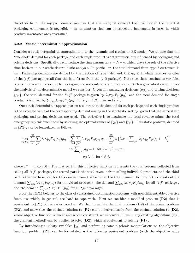
3.2.2 Static deterministic approximation

Consider a static deterministic approximation to the dynamic and stochastic ER model. We assume that the

“one-shot” demand for each package and each single product is deterministic but influenced by packaging and

pricing decisions. Specifically, we introduce the time parameter τ = N−n, which plays the role of the effectivetime horizon in our static deterministic analysis. In particular, the total demand from type i customers is

λiτ . Packaging decisions are defined by the fraction of type i demand, 0 ≤ qij ≤ 1, which receives an offerof the (i-j) package (recall that this is different from the (j-i) package). Note that these continuous variables

represent a generalization of the packaging decisions introduced in Section 2. Such a generalization simplifies

the analysis of the deterministic model we consider. Given any packaging decisions {qij} and pricing decisions{pij}, the total demand for the “i-j” package is given by λiτqijF ij(pij), and the total demand for single

product i is given byPj 6=i λiτqijFij(pij), for i, j = 1, 2, ...,m and i 6= j.

Our static deterministic approximation assumes that the demand for each package and each single product

is the expected value of the corresponding demand arising in the stochastic setting, given that the same static

packaging and pricing decisions are used. The objective is to maximize the total revenue minus the total

emergency replenishment cost by selecting the optimal values of {qij} and {pij}. This static problem, denotedas (P1), can be formulated as follows:

maxqij ,pij

mXi=1

Xj 6=i

λiτqijF ij(pij)pij +mXi=1

Xj 6=i

λiτqijFij(pij)pi −mXi=1

bi

³λiτ +

Xj 6=i λjτqjiF ji(pji)− Ii

´+s.t.X

j 6=i qij = 1, for i = 1, 2, ...,m,

qij > 0, for i 6= j,

where x+ = max{x, 0}. The first part in this objective function represents the total revenue collected fromselling all “i-j” packages, the second part is the total revenue from selling individual products, and the third

part is the purchase cost for ERs derived from the fact that the total demand for product i consists of the

demandPj 6=i λiτqijFij(pij) for individual product i, the demand

Pj 6=i λiτqijF ij(pij) for all “i-j” packages,

and the demandPj 6=i λjτqjiF ji(pji) for all “j-i” packages.

Note that (P1) belongs to the class of constrained optimization problems with non-differentiable objective

functions, which, in general, are hard to cope with. Next we consider a modified problem (P2) that is

equivalent to (P1) but is easier to solve. We then formulate the dual problem (D2) of the primal problem

(P2), and show that the optimal solution to (P2) can be derived easily from the optimal solution to (D2),

whose objective function is linear and whose constraint set is convex. Thus, many existing algorithms (e.g.,

the gradient method) can be applied to solve (D2), which is equivalent to solving (P1) .

By introducing auxiliary variables {yi} and performing some algebraic manipulations on the objectivefunction, problem (P1) can be formulated as the following equivalent problem (with the objective value

12

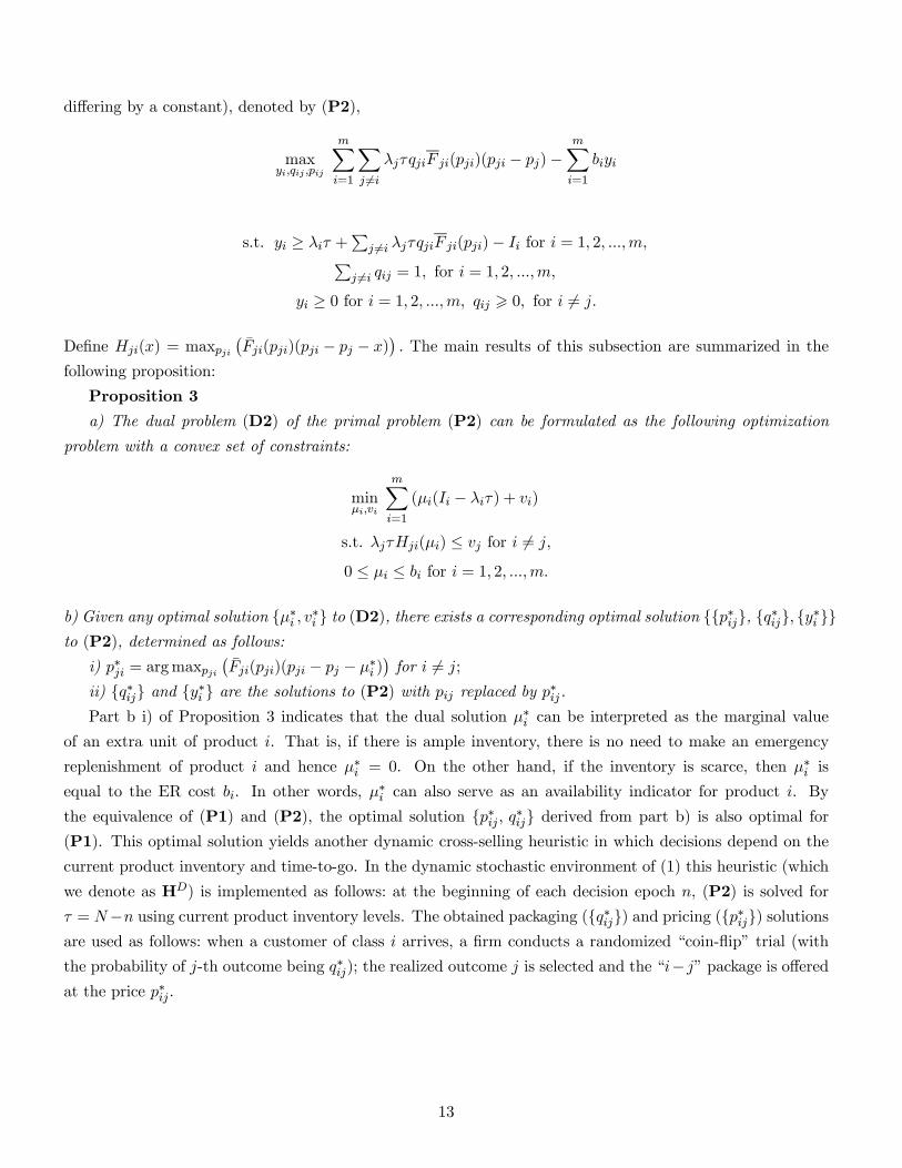
differing by a constant), denoted by (P2),

maxyi,qij ,pij

mXi=1

Xj 6=i

λjτqjiF ji(pji)(pji − pj)−mXi=1

biyi

s.t. yi ≥ λiτ +Pj 6=i λjτqjiF ji(pji)− Ii for i = 1, 2, ...,m,P

j 6=i qij = 1, for i = 1, 2, ...,m,

yi ≥ 0 for i = 1, 2, ...,m, qij > 0, for i 6= j.

Define Hji(x) = maxpji¡F̄ji(pji)(pji − pj − x)

¢. The main results of this subsection are summarized in the

following proposition:

Proposition 3

a) The dual problem (D2) of the primal problem (P2) can be formulated as the following optimization

problem with a convex set of constraints:

minµi,vi

mXi=1

(µi(Ii − λiτ) + vi)

s.t. λjτHji(µi) ≤ vj for i 6= j,0 ≤ µi ≤ bi for i = 1, 2, ...,m.

b) Given any optimal solution {µ∗i , v∗i } to (D2), there exists a corresponding optimal solution {{p∗ij}, {q∗ij}, {y∗i }}to (P2), determined as follows:

i) p∗ji = argmaxpji¡F̄ji(pji)(pji − pj − µ∗i )

¢for i 6= j;

ii) {q∗ij} and {y∗i } are the solutions to (P2) with pij replaced by p∗ij.Part b i) of Proposition 3 indicates that the dual solution µ∗i can be interpreted as the marginal value

of an extra unit of product i. That is, if there is ample inventory, there is no need to make an emergency

replenishment of product i and hence µ∗i = 0. On the other hand, if the inventory is scarce, then µ∗i isequal to the ER cost bi. In other words, µ

∗i can also serve as an availability indicator for product i. By

the equivalence of (P1) and (P2), the optimal solution {p∗ij , q∗ij} derived from part b) is also optimal for

(P1). This optimal solution yields another dynamic cross-selling heuristic in which decisions depend on the

current product inventory and time-to-go. In the dynamic stochastic environment of (1) this heuristic (which

we denote as HD) is implemented as follows: at the beginning of each decision epoch n, (P2) is solved for

τ = N−n using current product inventory levels. The obtained packaging ({q∗ij}) and pricing ({p∗ij}) solutionsare used as follows: when a customer of class i arrives, a firm conducts a randomized “coin-flip” trial (with

the probability of j-th outcome being q∗ij); the realized outcome j is selected and the “i− j” package is offeredat the price p∗ij .

13

3.2.3 A two-stage heuristic

Suppose that at the beginning of the n-th decision epoch the current inventory vector is I. Under the “two-

stage” approach, we simplify the packaging/pricing problem by assuming that there is no packaging in periods

n + 1 through N . Note that the number of type i customers arriving in each epoch is a Bernoulli random

variable with parameter λi and the number of type i customers arriving in all remaining N − n epochs is abinomial random variable Λi with parameters (λi, N−n).Then, the marginal value of an extra unit of productj 6= i can be expressed as

Vn+1 (I− ei)− Vn+1 (I− ei − ej) = bjE (min (Λj , Ij)−min (Λj , Ij − 1)) (14)

= bj Pr (Λj > Ij) = bjN−nXk=Ij

µN − nk

¶λkj (1− λj)

N−n−k .

The package price pTij for any (i, j) combination can be established from

∂Vn (I) /∂pij = fij (pij) (pi + Vn+1 (I− ei))− fij (pij) (pij + Vn+1 (I− ei − ej)) + F ij (pij) (15)

= −fij (pij) (pij − pi − (Vn+1 (I− ei)− Vn+1 (I− ei − ej))) + F ij (pij) = 0,

so that after substituting (14) to (15) and rearranging we obtain

pTij = pi + F ij¡pTij¢±fij¡pTij¢+ bj

XN−nk=Ij

µN − nk

¶λkj (1− λj)

N−n−k . (16)

Note that the expression for the myopic price pMij introduced earlier does not contain the last term appearing

in (16): pTij (T stands for the heuristically calculated “T”erminal value of inventory) is an upper bound on

pMij . At the same time, pTij is a lower bound on the optimal price since packaging in subsequent periods is not

accounted for. Also note that the value of pTij explicitly depends on the inventory of product j.

The packaging complement for product i is then determined as follows. Suppose that customer i arrives

and we decide not to offer any package. Then we earn pi + Vn+1 (I− ei) . The incremental value (denoted by∆ij) of offering the package “i− j” can be calculated as follows:

∆ij =¡Fij¡pTij¢(pi + Vn+1 (I− ei)) + F ij

¡pTij¢ ¡pTij + Vn+1 (I− ei − ej)

¢¢− (pi + Vn+1 (I− ei))= F ij

¡pTij¢ ¡pTij − pi − (Vn+1 (I− ei)− Vn+1 (I− ei − ej))

¢= F ij

¡pTij¢µpTij − pi − bj

PN−nk=Ij

µN − nk

¶λkj (1− λj)

N−n−k¶

=¡F ij

¡pTij¢¢2.

fij¡pTij¢(from (16)).

Hence, we propose the following dynamic packaging/pricing heuristic HT : when a customer of type i arrives,

we calculate pTij for all j using (16). Then, the values of ∆ij are computed for all j and the index of the

14

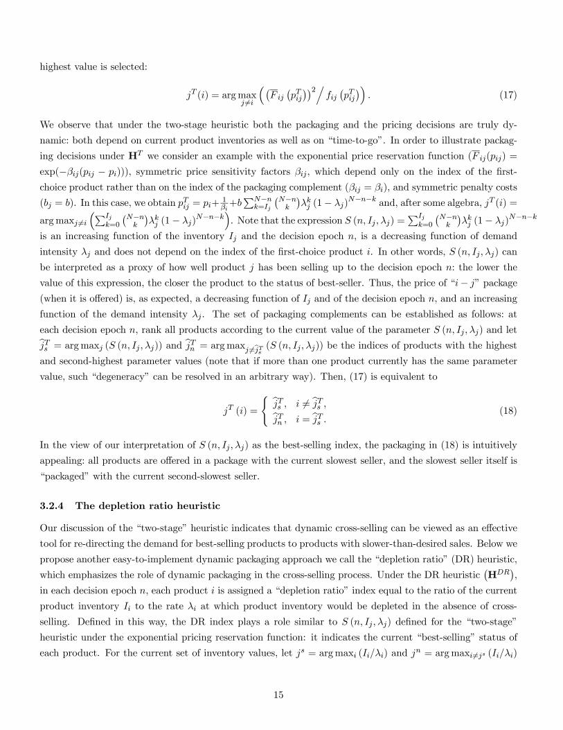
highest value is selected:

jT (i) = argmaxj 6=i

³¡F ij

¡pTij¢¢2.

fij¡pTij¢´. (17)

We observe that under the two-stage heuristic both the packaging and the pricing decisions are truly dy-

namic: both depend on current product inventories as well as on “time-to-go”. In order to illustrate packag-

ing decisions under HT we consider an example with the exponential price reservation function (F ij(pij) =

exp(−βij(pij − pi))), symmetric price sensitivity factors βij , which depend only on the index of the first-choice product rather than on the index of the packaging complement (βij = βi), and symmetric penalty costs

(bj = b). In this case, we obtain pTij = pi+

1βi+bPN−nk=Ij

¡N−nk

¢λkj (1− λj)

N−n−k and, after some algebra, jT (i) =

argmaxj 6=i³PIj

k=0

¡N−nk

¢λkj (1− λj)

N−n−k´. Note that the expression S (n, Ij ,λj) =

PIjk=0

¡N−nk

¢λkj (1− λj)

N−n−k

is an increasing function of the inventory Ij and the decision epoch n, is a decreasing function of demand

intensity λj and does not depend on the index of the first-choice product i. In other words, S (n, Ij ,λj) can

be interpreted as a proxy of how well product j has been selling up to the decision epoch n: the lower the

value of this expression, the closer the product to the status of best-seller. Thus, the price of “i− j” package(when it is offered) is, as expected, a decreasing function of Ij and of the decision epoch n, and an increasing

function of the demand intensity λj . The set of packaging complements can be established as follows: at

each decision epoch n, rank all products according to the current value of the parameter S (n, Ij ,λj) and letbjTs = argmaxj (S (n, Ij ,λj)) and bjTn = argmaxj 6=bjTs (S (n, Ij ,λj)) be the indices of products with the highestand second-highest parameter values (note that if more than one product currently has the same parameter

value, such “degeneracy” can be resolved in an arbitrary way). Then, (17) is equivalent to

jT (i) =

( bjTs , i 6= bjTs ,bjTn , i = bjTs . (18)

In the view of our interpretation of S (n, Ij ,λj) as the best-selling index, the packaging in (18) is intuitively

appealing: all products are offered in a package with the current slowest seller, and the slowest seller itself is

“packaged” with the current second-slowest seller.

3.2.4 The depletion ratio heuristic

Our discussion of the “two-stage” heuristic indicates that dynamic cross-selling can be viewed as an effective

tool for re-directing the demand for best-selling products to products with slower-than-desired sales. Below we

propose another easy-to-implement dynamic packaging approach we call the “depletion ratio” (DR) heuristic,

which emphasizes the role of dynamic packaging in the cross-selling process. Under the DR heuristic¡HDR

¢,

in each decision epoch n, each product i is assigned a “depletion ratio” index equal to the ratio of the current

product inventory Ii to the rate λi at which product inventory would be depleted in the absence of cross-

selling. Defined in this way, the DR index plays a role similar to S (n, Ij ,λj) defined for the “two-stage”

heuristic under the exponential pricing reservation function: it indicates the current “best-selling” status of

each product. For the current set of inventory values, let js = argmaxi (Ii/λi) and jn = argmaxi6=js (Ii/λi)

15

be the indices of the slowest-selling and the second slowest-selling products, respectively. Then, the dynamic

packaging decisions under the DR approach can be described as follows:

jDR (i) =

(js, i 6= js,jn, i = js.

(19)

The intuition behind the choice of the cross-selling complement in (19) is similar to the intuition behind (18):

every product is “packaged” with the current slowest seller, while the slowest seller itself is packaged with

the current second-slowest-selling product. Note that the DR approach does not restrict the choice of the

package pricing policy and can be combined with simple static pricing or sophisticated best-choice dynamic

pricing. In particular, in our analysis below we consider two cross-selling policies based on DR packaging: the

“myopic” DR policy (HDRM), which complements DR packaging with the myopic pricing defined by (13), and

the “optimal” DR policy (HDRO), which selects the best pricing under DR packaging by solving the variant

of (1) with packaging complements determined by (19).

Despite the intuitive nature of DR packaging, an analytical characterization of sufficient conditions for

its optimality is hard to obtain, except in rather restrictive settings. Below we provide an example of such

conditions under static pricing in a symmetric product environment:

Proposition 4

Let λi = λ, pi = p, bi = b, pij = q, p < q < p + b, and F ij(pij) = γ for any j 6= i and i, j = 1, 2, ...,m.

Then, DR packaging is optimal for any decision epoch n = 1, ..., N .

Proposition 4 considers the setting in which product packages are being sold at a fixed price and the

products differ only in their inventory values. While Proposition 4 indicates the potential effectiveness of the

DR packaging approach in nearly symmetric environments with static package pricing, its performance in

more typical settings needs to be evaluated numerically.

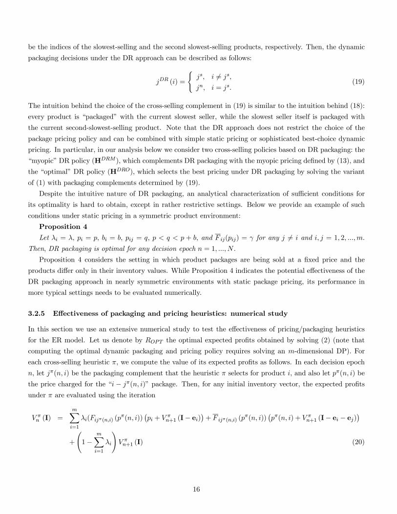
3.2.5 Effectiveness of packaging and pricing heuristics: numerical study

In this section we use an extensive numerical study to test the effectiveness of pricing/packaging heuristics

for the ER model. Let us denote by ROPT the optimal expected profits obtained by solving (2) (note that

computing the optimal dynamic packaging and pricing policy requires solving an m-dimensional DP). For

each cross-selling heuristic π, we compute the value of its expected profits as follows. In each decision epoch

n, let jπ(n, i) be the packaging complement that the heuristic π selects for product i, and also let pπ(n, i) be

the price charged for the “i − jπ(n, i)” package. Then, for any initial inventory vector, the expected profitsunder π are evaluated using the iteration

V πn (I) =

mXi=1

λi(Fijπ(n,i) (pπ(n, i))

¡pi + V

πn+1 (I− ei)

¢+ F ijπ(n,i) (p

π(n, i))¡pπ(n, i) + V π

n+1 (I− ei − ej)¢

+

Ã1−

mXi=1

λi

!V πn+1 (I) (20)

16

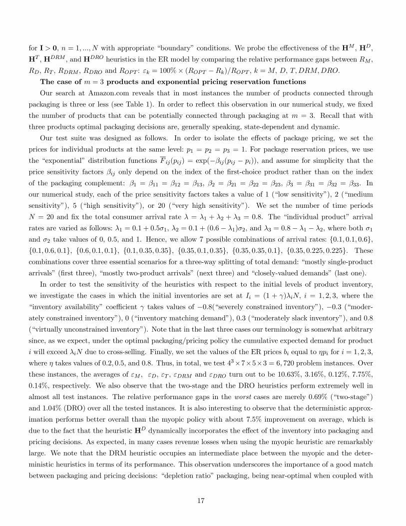
for I > 0, n = 1, ..., N with appropriate “boundary” conditions. We probe the effectiveness of the HM , HD,

HT , HDRM , and HDRO heuristics in the ER model by comparing the relative performance gaps between RM ,

RD, RT , RDRM , RDRO and ROPT : εk = 100%× (ROPT −Rk)/ROPT , k =M, D, T,DRM,DRO.The case of m = 3 products and exponential pricing reservation functions

Our search at Amazon.com reveals that in most instances the number of products connected through

packaging is three or less (see Table 1). In order to reflect this observation in our numerical study, we fixed

the number of products that can be potentially connected through packaging at m = 3. Recall that with

three products optimal packaging decisions are, generally speaking, state-dependent and dynamic.

Our test suite was designed as follows. In order to isolate the effects of package pricing, we set the

prices for individual products at the same level: p1 = p2 = p3 = 1. For package reservation prices, we use

the “exponential” distribution functions F ij(pij) = exp(−βij(pij − pi)), and assume for simplicity that theprice sensitivity factors βij only depend on the index of the first-choice product rather than on the index

of the packaging complement: β1 = β11 = β12 = β13, β2 = β21 = β22 = β23, β3 = β31 = β32 = β33. In

our numerical study, each of the price sensitivity factors takes a value of 1 (“low sensitivity”), 2 (“medium

sensitivity”), 5 (“high sensitivity”), or 20 (“very high sensitivity”). We set the number of time periods

N = 20 and fix the total consumer arrival rate λ = λ1 + λ2 + λ3 = 0.8. The “individual product” arrival

rates are varied as follows: λ1 = 0.1 + 0.5σ1, λ2 = 0.1 + (0.6− λ1)σ2, and λ3 = 0.8− λ1 − λ2, where both σ1

and σ2 take values of 0, 0.5, and 1. Hence, we allow 7 possible combinations of arrival rates: {0.1, 0.1, 0.6},{0.1, 0.6, 0.1}, {0.6, 0.1, 0.1}, {0.1, 0.35, 0.35}, {0.35, 0.1, 0.35}, {0.35, 0.35, 0.1}, {0.35, 0.225, 0.225}. These

combinations cover three essential scenarios for a three-way splitting of total demand: “mostly single-product

arrivals” (first three), “mostly two-product arrivals” (next three) and “closely-valued demands” (last one).

In order to test the sensitivity of the heuristics with respect to the initial levels of product inventory,

we investigate the cases in which the initial inventories are set at Ii = (1 + γ)λiN, i = 1, 2, 3, where the

“inventory availability” coefficient γ takes values of −0.8(“severely constrained inventory”), −0.3 (“moder-ately constrained inventory”), 0 (“inventory matching demand”), 0.3 (“moderately slack inventory”), and 0.8

(“virtually unconstrained inventory”). Note that in the last three cases our terminology is somewhat arbitrary

since, as we expect, under the optimal packaging/pricing policy the cumulative expected demand for product

i will exceed λiN due to cross-selling. Finally, we set the values of the ER prices bi equal to ηpi for i = 1, 2, 3,

where η takes values of 0.2, 0.5, and 0.8. Thus, in total, we test 43×7×5×3 = 6, 720 problem instances. Overthese instances, the averages of εM , εD, εT , εDRM and εDRO turn out to be 10.63%, 3.16%, 0.12%, 7.75%,

0.14%, respectively. We also observe that the two-stage and the DRO heuristics perform extremely well in

almost all test instances. The relative performance gaps in the worst cases are merely 0.69% (“two-stage”)

and 1.04% (DRO) over all the tested instances. It is also interesting to observe that the deterministic approx-

imation performs better overall than the myopic policy with about 7.5% improvement on average, which is

due to the fact that the heuristic HD dynamically incorporates the effect of the inventory into packaging and

pricing decisions. As expected, in many cases revenue losses when using the myopic heuristic are remarkably

large. We note that the DRM heuristic occupies an intermediate place between the myopic and the deter-

ministic heuristics in terms of its performance. This observation underscores the importance of a good match

between packaging and pricing decisions: “depletion ratio” packaging, being near-optimal when coupled with

17

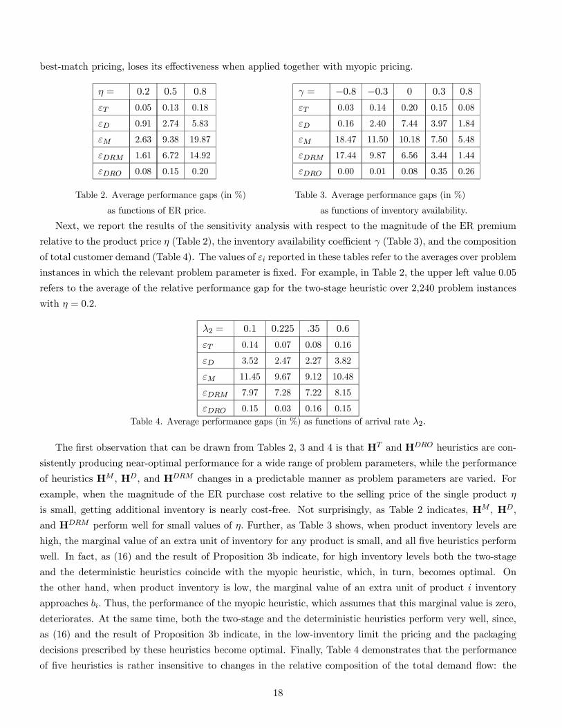
best-match pricing, loses its effectiveness when applied together with myopic pricing.

η = 0.2 0.5 0.8

εT 0.05 0.13 0.18

εD 0.91 2.74 5.83

εM 2.63 9.38 19.87

εDRM 1.61 6.72 14.92

εDRO 0.08 0.15 0.20

γ = −0.8 −0.3 0 0.3 0.8

εT 0.03 0.14 0.20 0.15 0.08

εD 0.16 2.40 7.44 3.97 1.84

εM 18.47 11.50 10.18 7.50 5.48

εDRM 17.44 9.87 6.56 3.44 1.44

εDRO 0.00 0.01 0.08 0.35 0.26

Table 2. Average performance gaps (in %) Table 3. Average performance gaps (in %)

as functions of ER price. as functions of inventory availability.

Next, we report the results of the sensitivity analysis with respect to the magnitude of the ER premium

relative to the product price η (Table 2), the inventory availability coefficient γ (Table 3), and the composition

of total customer demand (Table 4). The values of εi reported in these tables refer to the averages over problem

instances in which the relevant problem parameter is fixed. For example, in Table 2, the upper left value 0.05

refers to the average of the relative performance gap for the two-stage heuristic over 2,240 problem instances

with η = 0.2.

λ2 = 0.1 0.225 .35 0.6

εT 0.14 0.07 0.08 0.16

εD 3.52 2.47 2.27 3.82

εM 11.45 9.67 9.12 10.48

εDRM 7.97 7.28 7.22 8.15

εDRO 0.15 0.03 0.16 0.15

Table 4. Average performance gaps (in %) as functions of arrival rate λ2.

The first observation that can be drawn from Tables 2, 3 and 4 is that HT and HDRO heuristics are con-

sistently producing near-optimal performance for a wide range of problem parameters, while the performance

of heuristics HM , HD, and HDRM changes in a predictable manner as problem parameters are varied. For

example, when the magnitude of the ER purchase cost relative to the selling price of the single product η

is small, getting additional inventory is nearly cost-free. Not surprisingly, as Table 2 indicates, HM , HD,

and HDRM perform well for small values of η. Further, as Table 3 shows, when product inventory levels are

high, the marginal value of an extra unit of inventory for any product is small, and all five heuristics perform

well. In fact, as (16) and the result of Proposition 3b indicate, for high inventory levels both the two-stage

and the deterministic heuristics coincide with the myopic heuristic, which, in turn, becomes optimal. On

the other hand, when product inventory is low, the marginal value of an extra unit of product i inventory

approaches bi. Thus, the performance of the myopic heuristic, which assumes that this marginal value is zero,

deteriorates. At the same time, both the two-stage and the deterministic heuristics perform very well, since,

as (16) and the result of Proposition 3b indicate, in the low-inventory limit the pricing and the packaging

decisions prescribed by these heuristics become optimal. Finally, Table 4 demonstrates that the performance

of five heuristics is rather insensitive to changes in the relative composition of the total demand flow: the

18

two-stage and DRO heuristics remain the best choice, followed by deterministic approximation, with myopic

policy a distant fourth. We obtain similar results for fixed values of λ1 and λ3.

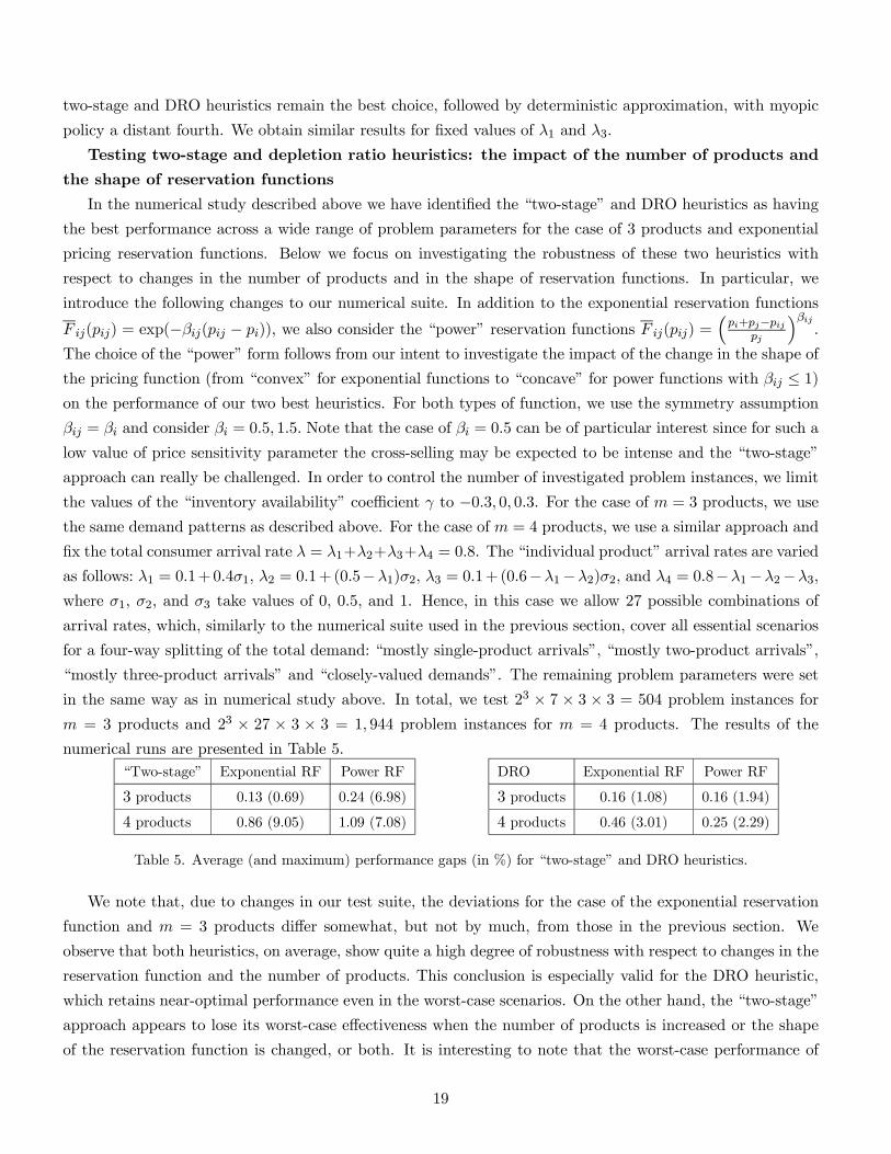
Testing two-stage and depletion ratio heuristics: the impact of the number of products and

the shape of reservation functions

In the numerical study described above we have identified the “two-stage” and DRO heuristics as having

the best performance across a wide range of problem parameters for the case of 3 products and exponential

pricing reservation functions. Below we focus on investigating the robustness of these two heuristics with

respect to changes in the number of products and in the shape of reservation functions. In particular, we

introduce the following changes to our numerical suite. In addition to the exponential reservation functions

F ij(pij) = exp(−βij(pij − pi)), we also consider the “power” reservation functions F ij(pij) =³pi+pj−pij

pj

´βij.

The choice of the “power” form follows from our intent to investigate the impact of the change in the shape of

the pricing function (from “convex” for exponential functions to “concave” for power functions with βij ≤ 1)on the performance of our two best heuristics. For both types of function, we use the symmetry assumption

βij = βi and consider βi = 0.5, 1.5. Note that the case of βi = 0.5 can be of particular interest since for such a

low value of price sensitivity parameter the cross-selling may be expected to be intense and the “two-stage”

approach can really be challenged. In order to control the number of investigated problem instances, we limit

the values of the “inventory availability” coefficient γ to −0.3, 0, 0.3. For the case of m = 3 products, we use

the same demand patterns as described above. For the case of m = 4 products, we use a similar approach and

fix the total consumer arrival rate λ = λ1+λ2+λ3+λ4 = 0.8. The “individual product” arrival rates are varied

as follows: λ1 = 0.1+0.4σ1, λ2 = 0.1+(0.5−λ1)σ2, λ3 = 0.1+(0.6−λ1−λ2)σ2, and λ4 = 0.8−λ1−λ2−λ3,

where σ1, σ2, and σ3 take values of 0, 0.5, and 1. Hence, in this case we allow 27 possible combinations of

arrival rates, which, similarly to the numerical suite used in the previous section, cover all essential scenarios

for a four-way splitting of the total demand: “mostly single-product arrivals”, “mostly two-product arrivals”,

“mostly three-product arrivals” and “closely-valued demands”. The remaining problem parameters were set

in the same way as in numerical study above. In total, we test 23 × 7 × 3 × 3 = 504 problem instances for

m = 3 products and 23 × 27 × 3 × 3 = 1, 944 problem instances for m = 4 products. The results of the

numerical runs are presented in Table 5.

“Two-stage” Exponential RF Power RF

3 products 0.13 (0.69) 0.24 (6.98)

4 products 0.86 (9.05) 1.09 (7.08)

DRO Exponential RF Power RF

3 products 0.16 (1.08) 0.16 (1.94)

4 products 0.46 (3.01) 0.25 (2.29)

Table 5. Average (and maximum) performance gaps (in %) for “two-stage” and DRO heuristics.

We note that, due to changes in our test suite, the deviations for the case of the exponential reservation

function and m = 3 products differ somewhat, but not by much, from those in the previous section. We

observe that both heuristics, on average, show quite a high degree of robustness with respect to changes in the

reservation function and the number of products. This conclusion is especially valid for the DRO heuristic,

which retains near-optimal performance even in the worst-case scenarios. On the other hand, the “two-stage”

approach appears to lose its worst-case effectiveness when the number of products is increased or the shape

of the reservation function is changed, or both. It is interesting to note that the worst-case performance of

19

the two-stage heuristic is observed in problem instances with βi = 0.5 and η = 0.8, i.e., the instances in which

1) consumers are willing to accept high package prices (for both types of reservation functions) and 2) the

out-of-stock products are costly to replenish. It is intuitive that the heuristic which neglects “future” cross-

selling opportunities does not perform well in cases in which cross-selling is readily accepted by customers.

This performance gap opens up dramatically when the number of cross-selling choices for each product is

increased from 2 (m = 3) to 3 (m = 4). The high cost of replenishment further accentuates the profit loss

resulting from the use of an ineffective cross-selling approach.

The ultimate choice between the DRO and the “two-stage” heuristics may depend on the specific features

of the business environment in which the firm operates. On the one hand, if the nature of the firm’s inventory

allows it to limit the number of likely complements for each product to 2, the firm may be advised to use the

“two stage” approach as long as its customers are relatively sensitive to package prices: the pricing policies

under “two-stage” approach are much easier to compute than those under the DRO heuristic (which requires

solving a number of optimization problems at each decision epoch). On the other hand, the DRO may be a

much more effective policy in cases in which the number of products is high or the estimated customer price

sensitivity for product packages is low.

4 The Lost Sales model

Although in some cases it is possible to procure an out-of-stock product, in a variety of situations this might

prove impossible or too costly. For example, when cross-selling travel services, there might not be seats

available on the requested route. Hence, it will be necessary to deny the customer’s request. To address

this issue, we consider an alternative setting in which there is no opportunity to replenish inventory and a

customer request is simply denied in the case of a stock-out. Similarly to the previous section, it is convenient

to introduce the sets of indices An to denote products that have at least one unit of inventory at the beginning

of the n-th decision epoch. Then, under the LS model, the generalization of (1) is given by

Vn (I) =Xi∈An

λi maxj 6=i, j∈An

µmaxpij

¡Fij (pij) (pi + Vn+1 (I− ei)) + F ij (pij) (pij + Vn+1 (I− ei − ej))

¢¶

+

Ã1−

Xi∈An

λi

!Vn+1 (I) . (21)

As (21) indicates, the “lost sales” feature of the inventory dynamics is reflected in the fact that the set of

product indices that actively participate in the DP transformation on the right-hand side of (1) is “shrinking”

as time passes.

4.1 Dynamic pricing under the static packaging

As indicated earlier, in the general case the LS model possesses few structural properties. However, the two-

product case is somewhat more amenable to analysis. Hence, we begin our analysis with this simpler case.

20

Under the LS model, when a company runs out of inventory for one of the products, we obtain

Vn(I1, 0) = λ1 (p1 + Vn+1(I1 − 1, 0)) + (1− λ1)Vn+1(I1, 0), (22)

for I1 ≥ 1, n = 1, ..., N and

Vn(0, I2) = λ2 (p2 + Vn+1(0, I2 − 1)) + (1− λ2)Vn+1(0, I2), (23)

for I2 ≥ 1, n = 1, ..., N . In addition, when the inventories of both products are depleted, we have

Vn(0, 0) = 0, n = 1, ..., N. (24)

Using the induction over the time index n, we can formalize the structural properties of the LS model in a

two-product case:

Proposition 5

a) The optimal expected revenue Vn(I1, I2) is a non-decreasing function of I1 and I2, respectively, for any

n = 1, ..., N :

Vn(I1 + 1, I2)− Vn(I1, I2) ≥ 0, Vn(I1, I2 + 1)− Vn(I1, I2) ≥ 0. (25)

b) The optimal expected revenue Vn(I1, I2) is a supermodular function of (I1, I2), for any n = 1, ..., N :

Vn(I1 + 1, I2 + 1)− Vn(I1, I2 + 1) ≥ Vn(I1 + 1, I2)− Vn(I1, I2). (26)

c) The optimal package price p∗ij(I1, I2, n) is non-decreasing in Ii, for (i, j) = (1, 2) and (2, 1):

p∗12(I1 + 1, I2, n) ≥ p∗12(I1, I2, n), n = 1, ..., N,

p∗21(I1, I2 + 1, n) ≥ p∗21(I1, I2, n), n = 1, ..., N. (27)

The statement of part a) of Proposition 5 is intuitively appealing and is similar to those established in the

literature on single-product pricing (see, e.g., Gallego and van Ryzin [16], and Federgruen and Heching [13]).

The statement of part b) can be rationalized as follows: the higher the inventory level for product j, the more

opportunities there are for selling product i. Thus, the marginal profit from adding one unit of product i

increases as the inventory level of product j increases. Note that part b) is in sharp contrast to the ER model

in which the optimal value function was separable in inventories of all products and hence supermodularity

held trivially as an equality in (26).The intuition behind Proposition 5c can be explained as follows: the larger

the inventory of product i, the more opportunities there will be to sell this product in the future. Therefore,

the package offered to a customer requesting product i can be priced high as there will be other opportunities

in the future to sell the same package. This result should be contrasted with related results in single-product

revenue management where larger product inventory typically leads to lower price (see, e.g., Gallego and van

Ryzin [16]).

21

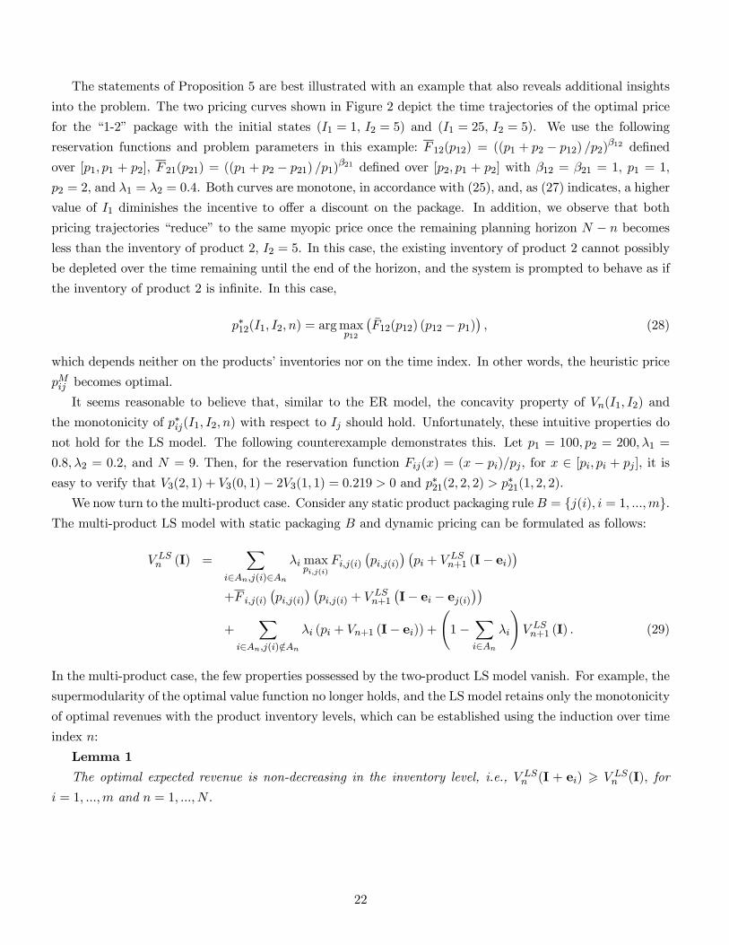
The statements of Proposition 5 are best illustrated with an example that also reveals additional insights

into the problem. The two pricing curves shown in Figure 2 depict the time trajectories of the optimal price

for the “1-2” package with the initial states (I1 = 1, I2 = 5) and (I1 = 25, I2 = 5). We use the following

reservation functions and problem parameters in this example: F 12(p12) = ((p1 + p2 − p12) /p2)β12 definedover [p1, p1 + p2], F 21(p21) = ((p1 + p2 − p21) /p1)β21 defined over [p2, p1 + p2] with β12 = β21 = 1, p1 = 1,

p2 = 2, and λ1 = λ2 = 0.4. Both curves are monotone, in accordance with (25), and, as (27) indicates, a higher

value of I1 diminishes the incentive to offer a discount on the package. In addition, we observe that both

pricing trajectories “reduce” to the same myopic price once the remaining planning horizon N − n becomesless than the inventory of product 2, I2 = 5. In this case, the existing inventory of product 2 cannot possibly

be depleted over the time remaining until the end of the horizon, and the system is prompted to behave as if

the inventory of product 2 is infinite. In this case,

p∗12(I1, I2, n) = argmaxp12

¡F̄12(p12) (p12 − p1)

¢, (28)

which depends neither on the products’ inventories nor on the time index. In other words, the heuristic price

pMij becomes optimal.

It seems reasonable to believe that, similar to the ER model, the concavity property of Vn(I1, I2) and

the monotonicity of p∗ij(I1, I2, n) with respect to Ij should hold. Unfortunately, these intuitive properties donot hold for the LS model. The following counterexample demonstrates this. Let p1 = 100, p2 = 200,λ1 =

0.8,λ2 = 0.2, and N = 9. Then, for the reservation function Fij(x) = (x − pi)/pj , for x ∈ [pi, pi + pj ], it iseasy to verify that V3(2, 1) + V3(0, 1)− 2V3(1, 1) = 0.219 > 0 and p∗21(2, 2, 2) > p∗21(1, 2, 2).

We now turn to the multi-product case. Consider any static product packaging ruleB = {j(i), i = 1, ...,m}.The multi-product LS model with static packaging B and dynamic pricing can be formulated as follows:

V LSn (I) =X

i∈An,j(i)∈Anλi maxpi,j(i)

Fi,j(i)¡pi,j(i)

¢ ¡pi + V

LSn+1 (I− ei)

¢+F i,j(i)

¡pi,j(i)

¢ ¡pi,j(i) + V

LSn+1

¡I− ei − ej(i)

¢¢+

Xi∈An,j(i)/∈An

λi (pi + Vn+1 (I− ei)) +Ã1−

Xi∈An

λi

!V LSn+1 (I) . (29)

In the multi-product case, the few properties possessed by the two-product LS model vanish. For example, the

supermodularity of the optimal value function no longer holds, and the LS model retains only the monotonicity

of optimal revenues with the product inventory levels, which can be established using the induction over time

index n:

Lemma 1

The optimal expected revenue is non-decreasing in the inventory level, i.e., V LSn (I + ei) > V LSn (I), for

i = 1, ...,m and n = 1, ..., N .

22

4.2 Heuristic approaches

Since even the stand-alone dynamic pricing problem under the LS model is rather intractable, there is little

hope of efficiently solving the dynamic pricing/packaging problem without the use of heuristics. Hence, it

is desirable to know how much we might lose by implementing a simple static packaging policy. Below we

derive upper and lower bounds for the expected profit under the LS model with static packaging and dynamic

pricing. Using these two bounds, we identify situations in which expected revenues are relatively insensitive

to the choice of a particular static packaging scheme.

Definition 2

Let Lin(I) be the function satisfying the following recursive relation:

Lin(I) = λi¡pi + L

in+1 (I − 1)

¢+ (1− λi)L

in+1 (I) , (30)

for I > 1, and Lin(0) = 0, for i = 1, ...,m, and n = 1, ..., N , while LiN+1(I) = 0.Definition 3

Let U in(I) be the function satisfying the following recursive relation:

U in(I) = λi

³pi + U

in+1 (I − 1) + F i,j(i)(pMi,j(i))(pMi,j(i) − pi)

´+ (1− λi)U

in+1 (I) , (31)

for I > 1, and U in(0) = 0, for i = 1, ...,m, and n = 1, ..., N , while U iN+1(I) = 0.Define Ln(I) =

Pmi=1 L

in(Ii) and Un(I) =

Pmi=1 U

in(Ii). Note that Ln(I) is the expected revenue under the

LS model with no packaging. The following proposition uses the induction over n to show that Ln(I) and

Un(I) are a lower bound and an upper bound, respectively, for the optimal expected revenue VLSn (I) in the

LS model.

Proposition 6

a) Ln(I) ≤ V LSn (I) ≤ Un(I), for n = 1, ..., N .b) For n = 1, ..., N ,

V LSn (I)− Ln (I)Ln (I)

≤ max½pj(i)

pi

¯̄̄̄i = 1, ...,m

¾. (32)

Note that the upper bound given in part b) of Proposition 6 is independent of customer reservation prices

and arrival processes. If each product is significantly more expensive than its packaging complement, then

the bound in (32) is tight, implying that the impact of the packaging decision on expected profit is negligible.

Given the price of each product, we can now easily compute the upper bound for each packaging topology.

Thus, without the demand information, we are able to identify the packaging configurations with the tight

upper bound. Consider an example in which (p1, p2, p3) = (100, 10, 1) and product 1 is packaged with product

2 and product 2 with product 3 (product 3 is not packaged with any other product). According to (32), under

this packaging configuration, the highest possible revenue is at most 10% above the revenue achieved in the

absence of cross-selling.

Even with static packaging, the computation of the optimal price under the LS assumption requires solving

23

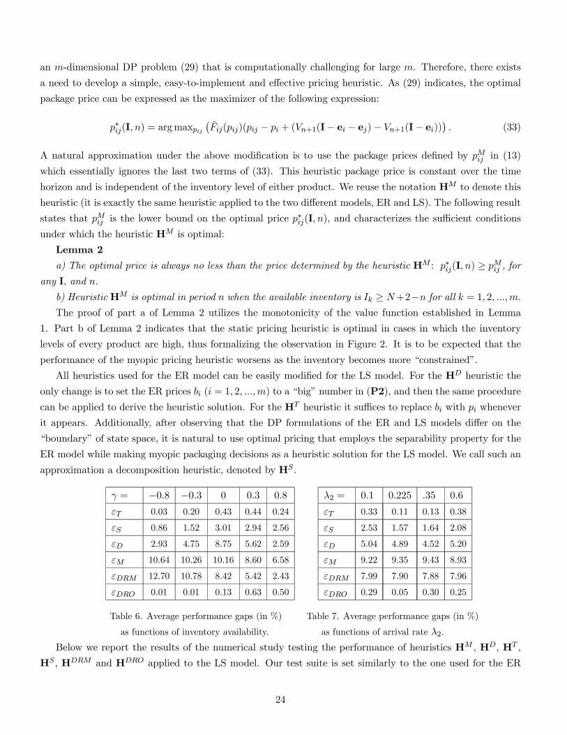
an m-dimensional DP problem (29) that is computationally challenging for large m. Therefore, there exists

a need to develop a simple, easy-to-implement and effective pricing heuristic. As (29) indicates, the optimal

package price can be expressed as the maximizer of the following expression:

p∗ij(I, n) = argmaxpij¡F̄ij(pij)(pij − pi + (Vn+1(I− ei − ej)− Vn+1(I− ei))

¢. (33)

A natural approximation under the above modification is to use the package prices defined by pMij in (13)

which essentially ignores the last two terms of (33). This heuristic package price is constant over the time

horizon and is independent of the inventory level of either product. We reuse the notation HM to denote this

heuristic (it is exactly the same heuristic applied to the two different models, ER and LS). The following result

states that pMij is the lower bound on the optimal price p∗ij(I, n), and characterizes the sufficient conditions

under which the heuristic HM is optimal:

Lemma 2

a) The optimal price is always no less than the price determined by the heuristic HM : p∗ij(I, n) ≥ pMij , forany I, and n.

b) HeuristicHM is optimal in period n when the available inventory is Ik ≥ N+2−n for all k = 1, 2, ...,m.The proof of part a of Lemma 2 utilizes the monotonicity of the value function established in Lemma

1. Part b of Lemma 2 indicates that the static pricing heuristic is optimal in cases in which the inventory

levels of every product are high, thus formalizing the observation in Figure 2. It is to be expected that the

performance of the myopic pricing heuristic worsens as the inventory becomes more “constrained”.

All heuristics used for the ER model can be easily modified for the LS model. For the HD heuristic the

only change is to set the ER prices bi (i = 1, 2, ...,m) to a “big” number in (P2), and then the same procedure

can be applied to derive the heuristic solution. For the HT heuristic it suffices to replace bi with pi whenever

it appears. Additionally, after observing that the DP formulations of the ER and LS models differ on the

“boundary” of state space, it is natural to use optimal pricing that employs the separability property for the

ER model while making myopic packaging decisions as a heuristic solution for the LS model. We call such an

approximation a decomposition heuristic, denoted by HS.

γ = −0.8 −0.3 0 0.3 0.8

εT 0.03 0.20 0.43 0.44 0.24

εS 0.86 1.52 3.01 2.94 2.56

εD 2.93 4.75 8.75 5.62 2.59

εM 10.64 10.26 10.16 8.60 6.58

εDRM 12.70 10.78 8.42 5.42 2.43

εDRO 0.01 0.01 0.13 0.63 0.50

λ2 = 0.1 0.225 .35 0.6

εT 0.33 0.11 0.13 0.38

εS 2.53 1.57 1.64 2.08

εD 5.04 4.89 4.52 5.20

εM 9.22 9.35 9.43 8.93

εDRM 7.99 7.90 7.88 7.96

εDRO 0.29 0.05 0.30 0.25

Table 6. Average performance gaps (in %) Table 7. Average performance gaps (in %)

as functions of inventory availability. as functions of arrival rate λ2.

Below we report the results of the numerical study testing the performance of heuristics HM , HD, HT ,

HS, HDRM and HDRO applied to the LS model. Our test suite is set similarly to the one used for the ER

24

numerical study described above, except, naturally, for the absence of the ER prices bi. Thus, for the LS

model we test in total 43 × 7 × 5 = 2, 240 problem instances. Over these problem instances, the average

relative performance gaps for the four heuristics (εM , εD, εT , εS , εDRM and εDRO) are 9.25%, 4.93%, 0.27%,

2.18%, 7.95%, and 0.26%, respectively. Tables 6 and 7 indicate that, just as in the ER case, the two-stage

and DRO heuristics perform extremely well, with worst-case relative performance gaps of 1.8% and 1.55%.

Comparing Tables 3 and 6, we observe that the performance of the deterministic heuristic worsens in the LS

model, and the decomposition heuristic becomes the third-best performer.

5 Summary

In this paper we study the problem of dynamically cross-selling products on the Internet. While there are

related studies of static bundling and static cross-selling decisions, to the best of our knowledge there are

no studies that, like ours, consider cross-selling in the dynamic setting and identify it as an opportunity

complementary to single-product revenue management. The dynamic aspect of the cross-selling problem is

important since the Internet provides a truly dynamic environment that differs from the static setting of

the brick-and-mortar store in many aspects. These aspects are also found in the dynamic pricing/revenue

management literature, which we draw upon in our analysis. However, this literature has predominantly

focused on dynamic pricing for a single product and hence does not address dynamic pricing of product

packages under cross-selling.

Our findings can be concisely summarized in the following two tables. Table 8 characterizes the optimal

cross-selling approaches under different inventory levels of individual products. When inventory is ample (last

column) there is little need to account for product inventories when making cross-selling decisions: the main

driving force behind the optimal package price is consumer preferences. This is when myopic cross-selling

policies work well. If inventory is severely constrained (first column), revenue management through dynamic

cross-selling is beneficial in the ER model but much less so in the LS model. Understandably, the simple

myopic heuristic performs very poorly in this case. Finally, most benefits from dynamic cross-selling arise

when inventory is approximately equal to expected demand. In this case it is particularly important to have a

good heuristic solution. Indeed, from Tables 3 and 6 we can see that the performance of all heuristics worsens

for intermediate levels of inventory because of the impact of incorrect cross-selling decisions. However, the

two-stage and DRO heuristics are still good approximations of the optimal dynamic cross-selling policy.

Inventory¿Exp. Demand Inventory=Exp. Demand InventoryÀExp. DemandER model Dynamic cross-selling Myopic cross-selling

LS model No cross-selling Dynamic cross-selling Myopic cross-selling

Table 8. The optimal cross-selling approaches for different inventory levels.

Table 9 further illustrates our earlier observation that dynamic cross-selling is complementary to more

traditional single-product revenue management. While single-product revenue management is most effective

when product inventory is highly constrained, most benefits from dynamic cross-selling arise when product

inventory is approximately equal to expected demand. Therefore, a potentially fruitful direction for future

25

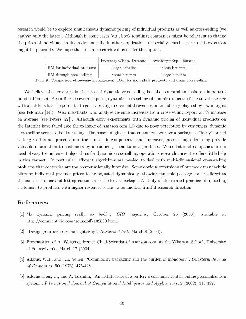
research would be to explore simultaneous dynamic pricing of individual products as well as cross-selling (we

analyze only the latter). Although in some cases (e.g., book retailing) companies might be reluctant to change

the prices of individual products dynamically, in other applications (especially travel services) this extension

might be plausible. We hope that future research will consider this option.

Inventory¿Exp. Demand Inventory=Exp. Demand

RM for individual products Large benefits Some benefits

RM through cross-selling Some benefits Large benefits

Table 9. Comparison of revenue management (RM) for individual products and using cross-selling.

We believe that research in the area of dynamic cross-selling has the potential to make an important

practical impact. According to several experts, dynamic cross-selling of non-air elements of the travel package

with air tickets has the potential to generate large incremental revenues in an industry plagued by low margins

(see Feldman [14]). Web merchants who analyze revenue increases from cross-selling report a 5% increase

on average (see Peters [27]). Although early experiments with dynamic pricing of individual products on

the Internet have failed (see the example of Amazon.com [1]) due to poor perception by customers, dynamic

cross-selling seems to be flourishing. The reason might be that customers perceive a package as “fairly” priced

as long as it is not priced above the sum of its components, and moreover, cross-selling offers may provide

valuable information to customers by introducing them to new products. While Internet companies are in

need of easy-to-implement algorithms for dynamic cross-selling, operations research currently offers little help

in this respect. In particular, efficient algorithms are needed to deal with multi-dimensional cross-selling

problems that otherwise are too computationally intensive. Some obvious extensions of our work may include

allowing individual product prices to be adjusted dynamically, allowing multiple packages to be offered to

the same customer and letting customers self-select a package. A study of the related practice of up-selling

customers to products with higher revenues seems to be another fruitful research direction.

References

[1] “Is dynamic pricing really so bad?”, CIO magazine, October 25 (2000), available at

http://comment.cio.com/soundoff/102500.html.

[2] “Design your own discount gateway”, Business Week, March 8 (2004).

[3] Presentation of A. Weigend, former Chief-Scientist of Amazon.com, at the Wharton School, University

of Pennsylvania, March 17 (2004).

[4] Adams, W.J., and J.L. Yellen, “Commodity packaging and the burden of monopoly”, Quarterly Journal

of Economics, 90 (1976), 475-498.

[5] Adomavicius, G., and A. Tuzhilin, “An architecture of e-butler: a consumer-centric online personalization

system”, International Journal of Computational Intelligence and Applications, 2 (2002), 313-327.

26

[6] Aviv, Y., and A. Pazgal. “A partially observed Markov decision process for dynamic pricing”, Working

Paper (2003), Washington University at St. Louis.

[7] Bertsimas, D.J., Mersereau, A.J., and N.R. Patel. Dynamic classification of online customers. Proceedings

of SIAM International Conference on Data Mining (2003).

[8] Bitran, G., and R. Caldentey, “Commissioned paper: an overview of pricing models for revenue manage-

ment”, Manufacturing and Service Operations Management, 5 (2003), 203-229.

[9] Elmaghraby, W., and P. Keskinocak, “Dynamic pricing in the presence of inventory considerations:

research overview, current practices, and future directions”, Management Science, 49 (2003), 1287-1309.

[10] Ernst, R., and P. Kouvelis, “The effect of selling packaged goods on inventory decisions”, Management

Science, 45 (1999), 1142-1155.

[11] E-tailing Group Inc. web page, http://www.e-tailing.com/.

[12] Federgruen, A., Groenevelt, H., and H.C. Tijms, “Coordinated replenishment in a multi-item inventory

system with compound Poisson demands”, Management Science, 30 (1984), 344-357.

[13] Federgruen, A., and A. Heching, “Combined pricing and inventory control under uncertainty”, Operations

Research, 47 (1999), 454-475.

[14] Feldman, J.M. “Package deal”, Air Transport World, 40, No.3 (2003), 40-42.

[15] Fuerderer, R., Herrmann, A., and G. Wuebker, editors, Optimal packaging: marketing strategies for

improving economic performance, Springer (1999).

[16] Gallego, G., and G. van Ryzin, “Optimal dynamic pricing of inventories with stochastic demand over

finite horizons”, Management Science, 40 (1994), 999-1020.

[17] Gallego, G., and G. van Ryzin. “A multiproduct dynamic pricing problem and its applications to network

yield management”, Operations Research, 45 (1997), 24-41.

[18] Hanson, W., and R.K. Martin, “Optimal package pricing”, Management Science, 36 (1990), 155-174.

[19] Kamakura, W.A., Wedel, M., de Rosa, F., and J.A. Mazzon. “Cross-selling through database marketing:

a mixed data factor analyzer for data augmentation and prediction”, International Journal of Research

in Marketing, 20 (2003), 45-65.

[20] Maglaras, C., and J. Meissner, “Dynamic pricing strategies for multi-product revenue management prob-

lems”, Working Paper (2003), Columbia University.

[21] McGill, J.I., and G. van Ryzin, “Revenue management: research overview and prospects”, Transportation

Science, 33, (1999), 233-256.

27

[22] Moe, W.W., and P.S. Fader. “Dynamic conversion behavior at e-commerce sites.” Management Science,

50, (2004), 326-335.

[23] Monahan, G.E., N.C. Petruzzi and W. Zhao, “The dynamic pricing problem from a newsvendor perspec-

tive”, Manufacturing & Service Operations Management, 6 (2004), 73-91.

[24] Nash, D., and A. Sterna-Karwat, “An application of DEA to measure branch cross selling efficiency.”

Computers and Operations Research, 23, No.4 (1996), 385-392.

[25] Netessine, S., and N. Rudi, “Supply chain choice on the Internet”, Working Paper (2003), University of

Pennsylvania, available at http://www.netessine.com.

[26] Padmanabhan, B., and A. Tuzhilin, “On the use of optimization for data mining: theoretical interactions

and eCRM opportunities”, Management Science, 49 (2003), 1327-1343.

[27] Peters, K. “May we suggest”. Internet Retailer, January (2004).

[28] Plambeck, E., and A. Ward, “A separation principle for assemble-to-order systems with expediting”,

Working Paper (2003), Stanford University.

[29] Rao, V.R., “Pricing models in marketing”, in Handbooks in operations research and management science:

Marketing by J. Eliashberg and G.L. Lilien, editors, North-Holland (1993).

[30] Scarf, H., “The optimality of (s, S) policies in the dynamic inventory problem”, Mathematical Models in

Social Sciences, K. Arrow, S. Karlin and P. Suppes, editors, Stanford University Press (1960).

[31] Stigler, G., “A note on block booking”, Reprinted in Organization of Industry, Chicago University Press

(1963).

[32] Stremersch, S., and G.J. Tellis, “Strategic packaging of products and prices: a new synthesis for market-

ing”, Journal of Marketing, 66 (2002), 55-72.

[33] Veinott, A.F., “On the optimality of (s, S) inventory policies: new conditions and a new proof”, SIAM

Journal of Applied Mathematics, 14 (1966), 1067-1083.

[34] Zhang, D., and W.L. Cooper. “Revenue management for parallel flights with customer choice behavior”,

Working Paper (2003), University of Minnesota.

[35] Zheng, Y.-S., “A simple proof for optimality of (s, S) policies in infinite-horizon inventory systems”,

Journal of Applied Probability, 28 (1991), 802-810.

[36] Zheng, Y.-S., “Optimal control policy for stochastic inventory systems with Markovian discount oppor-

tunities”, Operations Research, 42 (1994), 721-738.

[37] Ziya, S., H. Ayhan and R.D. Foley, “Relationship among three assumptions in revenue management”,

Operations Research, 52, (2004), 804-809.

28

AppendixProof of Proposition 1

For the proof of Proposition we need an additional result:

Lemma A1

Let gij(x) = maxy¡F̄ij(y)(y − x)

¢where 1 ≤ i 6= j ≤ m.

a) For any x1 ≥ 0 and x2 ≥ 0,

max (0, x2 − x1) ≥ gij(x1)− gij(x2) ≥ min (0, x2 − x1) . (34)

b) For any x1 ≥ x2 ≥ 0, let yk be the maximizer of gij(xk) (k = 1, 2). Then y1 ≥ y2.Proof of Lemma A1

Let yk be the maximizer of gij(xk) (k = 1, 2). We consider two cases: x1 ≥ x2 and x1 ≤ x2. If x1 ≥ x2,then by definition, gij(x2) = F̄ij(y2)(y2−x2) ≥ F̄ij(y1)(y1−x2) ≥ F̄ij(y1)(y1−x1) = gij(x1) ≥ F̄ij(y2)(y2−x1).This yields 0 ≤ gij(x2)− gij(x1) ≤ F̄ij(y2)(x1 − x2) ≤ x1 − x2 and F̄ij(y1) ≤ F̄ij(y2), i.e., y1 ≥ y2. If x1 ≤ x2,by symmetry, we have 0 ≤ gij(x1)− gij(x2) ≤ x2 − x1. Combining these two cases, we get (34). ¥

The statement trivially holds for n = N + 1. Using induction, suppose that for some n = 1, ..., N

Vn+1(I) =Pmi=1G

in+1(Ii). (35)

We need to prove that Vn(I) =Pmi=1G

in(Ii).

Vn(I)

=X

i∈An,j(i)∈Anλi

µpi + Vn+1(I− ei) + max

pi,j(i)

¡F̄i,j(i)(pi,j(i))

¡pi,j(i) − pi + Vn+1(I− ei − ej(i))− Vn+1(I− ei)

¢¢¶

+X

i∈An,j(i)/∈Anλi

µpi + Vn+1(I− ei) + max

pi,j(i)

¡F̄i,j(i)(pi,j(i))

¡pi,j(i) − pi − bj(i)

¢¢¶

+X

i/∈An,j(i)∈Anλi

µpi − bi + Vn+1(I) + max

pi,j(i)F̄i,j(i)(pi,j(i))

¡pi,j(i) − pi + Vn+1(I− ej(i))− Vn+1(I)

¢¶

+X

i/∈An,j(i)/∈Anλi

µpi − bi + Vn+1(I) + max

pi,j(i)F̄i,j(i)(pi,j(i))

¡pi,j(i) − pi − bj(i)

¢¶

+

Ã1−

mXi=1

λi

!Vn+1 (I)

=X

i∈An,j(i)∈Anλi

µpi +G

in+1(Ii − 1)−Gin+1(Ii) + maxpi,j(i)

F̄i,j(i)(pi,j(i))³pi,j(i) − pi +Gj(i)n+1(Ij(i) − 1)−Gj(i)n+1(Ij(i))

´¶

+X

i∈An,j(i)/∈Anλi

µpi +G

in+1(Ii − 1)−Gin+1(Ii) + maxpi,j(i)

F̄i,j(i)(pi,j(i))¡pi,j(i) − pi − bj(i)

¢¶

+X

i/∈An,j(i)∈Anλi

µpi − bi + max

pi,j(i)F̄i,j(i)(pi,j(i))

³pi,j(i) − pi +Gj(i)n+1(Ij(i) − 1)−Gj(i)n+1(Ij(i))

´¶

29

+X

i/∈An,j(i)/∈Anλi

µpi − bi + max

pi,j(i)F̄i,j(i)(pi,j(i))

¡pi,j(i) − pi − bj(i)

¢¶+

mXi=1

Gin+1(Ii) (from (35))

=mXi=1

Gin(Ii). (from (9))¥

Proof of Proposition 3

a) Following the standard Lagrangian procedure to derive the dual function q(µ, ν), we have

q(µ, ν) = maxq>0,y>0,pij>0

L(p, q, y, µ, ν)

= maxq>0,y>0,pij>0

( Pmi=1

Pj 6=i λjτqjiF ji(pji)(pji − pj)−

Pmi=1 biyi+Pm

i=1 µi[yi + Ii − λiτ −Pj 6=i λjτqjiF ji(pji)] +

Pmi=1 νi(1−

Pj 6=i qij)

)

= maxq>0,y>0,pij>0

( Pmi=1

Pj 6=i[λjτF ji(pji)(pji − pj − µi)− νj ]qji +

Pmi=1(µi − bi)yi+Pm

i=1[µi(Ii − λiτ) + νi]

)

= maxq>0,y>0

mXi=1

Xj 6=i[λjτHji(µi)− νj ]qji +

mXi=1

(µi − bi)yi +mXi=1

[µi(Ii − λiτ) + νi]

(36)

where the last equation follows from the definition of Hji(µi). Define Dq = {(µ, ν)|q(µ, v) < +∞}. It is easy tosee from (36) thatDq = {(µ, ν)|λjτHji(µi)−vj ≤ 0, for i 6= j, and µi ≤ bi}, and q(µ, ν) =

Pmi=1[µi(Ii−λiτ)+νi]

for (µ, ν) ∈ Dq. Hence the dual problem (D2) can be formulated as follows:

minµi,vj

: q(µ, v) =Xm

i=1[µi(Ii − λiτ) + vi]

s.t. λjτHji(µi) ≤ vj for i 6= j,0 ≤ µi ≤ bi for i = 1, 2, ...,m.

In order to show that the above constraint set is convex, it suffices to show that Hji(x) is convex for every

pair i 6= j. Recall that Hji(x) = maxpji¡F̄ji(pji)(pji − pj − x)

¢. Denote the maximizer of F̄ji(pji)(pji−pj−x)

by pji(x). Then from the first-order condition, we have

dF̄ji(pji)(pji − pj − x)dpji

|pji=pji(x) = 0. (37)

Taking the derivative of Hji(x), we have

dHji(x)

dx=dF̄ji(pji)(pji − pj − x)

dpji|pji=pji(x)

dpji(x)

dx− F̄ji(pji(x)) = −F̄ji(pji(x)), (38)

where the last equality follows from (37). Hence d2Hji(x)/dx2 = (dF (x)/dx) (dpji(x)/dx) > 0, which follows

from part b) of Lemma A1 and the fact that F (x) is a cumulative distribution function. This proves part a).

b) It is easy to ensure that the constraint set of (D2) is compact by imposing a finite bound on v. Hence,

the Weierstrass Theorem ensures the existence of the optimal solution to (D2). Denote the optimal solution

30

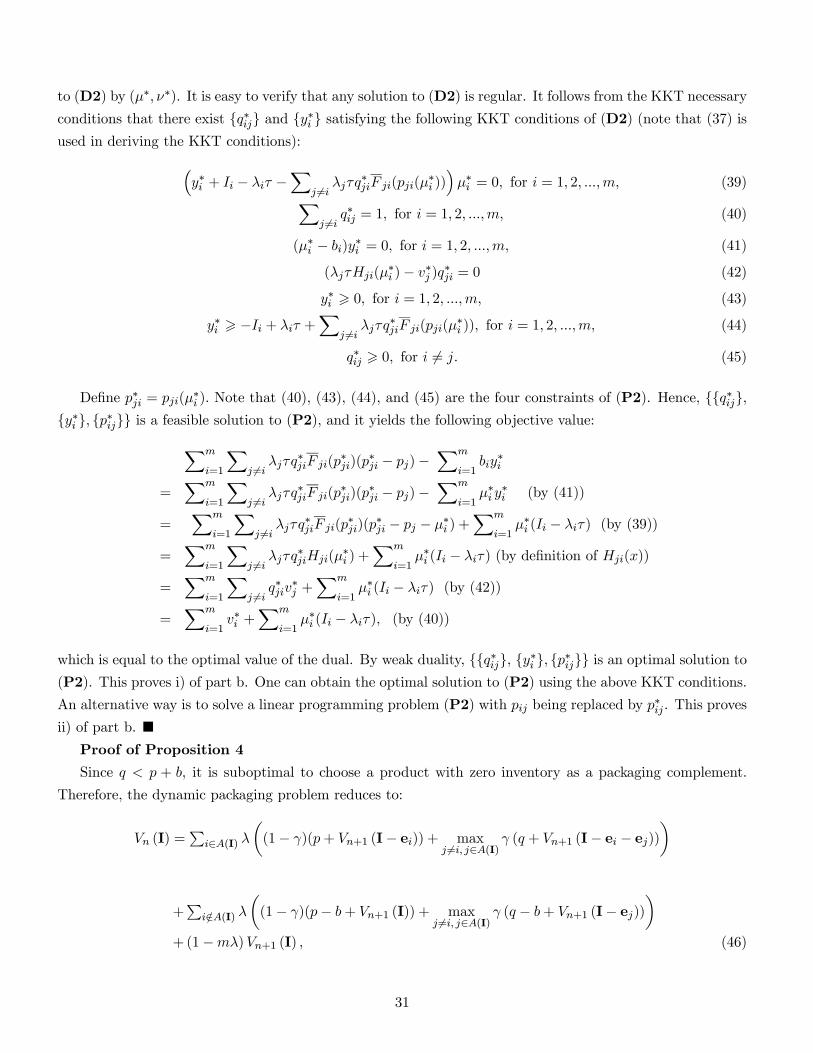
to (D2) by (µ∗, ν∗). It is easy to verify that any solution to (D2) is regular. It follows from the KKT necessaryconditions that there exist {q∗ij} and {y∗i } satisfying the following KKT conditions of (D2) (note that (37) isused in deriving the KKT conditions):³

y∗i + Ii − λiτ −X

j 6=i λjτq∗jiF ji(pji(µ

∗i ))´µ∗i = 0, for i = 1, 2, ...,m, (39)X

j 6=i q∗ij = 1, for i = 1, 2, ...,m, (40)

(µ∗i − bi)y∗i = 0, for i = 1, 2, ...,m, (41)

(λjτHji(µ∗i )− v∗j )q∗ji = 0 (42)

y∗i > 0, for i = 1, 2, ...,m, (43)

y∗i > −Ii + λiτ +X

j 6=i λjτq∗jiF ji(pji(µ

∗i )), for i = 1, 2, ...,m, (44)

q∗ij > 0, for i 6= j. (45)

Define p∗ji = pji(µ∗i ). Note that (40), (43), (44), and (45) are the four constraints of (P2). Hence, {{q∗ij},

{y∗i }, {p∗ij}} is a feasible solution to (P2), and it yields the following objective value:Xm

i=1

Xj 6=i λjτq

∗jiF ji(p

∗ji)(p

∗ji − pj)−

Xm

i=1biy

∗i

=Xm

i=1

Xj 6=i λjτq

∗jiF ji(p

∗ji)(p

∗ji − pj)−

Xm

i=1µ∗i y

∗i (by (41))

=Xm

i=1

Xj 6=i λjτq

∗jiF ji(p

∗ji)(p

∗ji − pj − µ∗i ) +

Xm

i=1µ∗i (Ii − λiτ) (by (39))

=Xm

i=1

Xj 6=i λjτq

∗jiHji(µ

∗i ) +

Xm

i=1µ∗i (Ii − λiτ) (by definition of Hji(x))

=Xm

i=1

Xj 6=i q

∗jiv∗j +

Xm

i=1µ∗i (Ii − λiτ) (by (42))

=Xm

i=1v∗i +

Xm

i=1µ∗i (Ii − λiτ), (by (40))

which is equal to the optimal value of the dual. By weak duality, {{q∗ij}, {y∗i }, {p∗ij}} is an optimal solution to(P2). This proves i) of part b. One can obtain the optimal solution to (P2) using the above KKT conditions.

An alternative way is to solve a linear programming problem (P2) with pij being replaced by p∗ij . This proves

ii) of part b. ¥Proof of Proposition 4

Since q < p + b, it is suboptimal to choose a product with zero inventory as a packaging complement.

Therefore, the dynamic packaging problem reduces to:

Vn (I) =Pi∈A(I) λ

µ(1− γ)(p+ Vn+1 (I− ei)) + max

j 6=i, j∈A(I)γ (q + Vn+1 (I− ei − ej))

¶

+Pi/∈A(I) λ

µ(1− γ)(p− b+ Vn+1 (I)) + max

j 6=i, j∈A(I)γ (q − b+ Vn+1 (I− ej))

¶+(1−mλ)Vn+1 (I) , (46)

31

where A (I) denotes products that have at least one unit of inventory at the beginning of the n-th decision

epoch when the inventory is I. The boundary condition is VN+1 (I) = 0. In order to prove the optimality of

the DR packaging, we need to show that Vn (I− ek) ≥ Vn (I− el) for any I = (I1, I2, ..., Im) with Ik ≥ Il ≥ 1and any n = 1, ..., N + 1. First, from the boundary condition, this inequality trivially holds when n = N + 1.

By induction, suppose it also holds up to some n+ 1, i.e.,

Vs (I− ek) ≥ Vs (I− el) , for any I = (I1, I2, ..., Im) with Ik ≥ Il ≥ 1 and s = n+ 1, ..., N + 1.(47)

We prove the desired result for two separate cases: Ik = Il = 1 and Ik > Il = 1 (the proof for the case of

Ik, Il > 1 follows similar steps).

Case 1: Ik = Il = 1.

Define B = {i|i 6= k, l,and Ii > 0} and C = {i|i 6= k, l,and Ii = 0}. Then A (I− ek) = B ∪ {l} andA (I− el) = B ∪ {k}. Note that for any i ∈ B, by (47), we have

maxj 6=i, j∈B

γ (q + Vn+1 (I− ei − ej−ek)) ≥ maxj 6=i, j∈B

γ (q + Vn+1 (I− ei − ej−el)) ,

which implies that

maxj 6=i, j∈B∪{l}

γ (q + Vn+1 (I− ei − ej−ek)) ≥ maxj 6=i, j∈B∪{k}

γ (q + Vn+1 (I− ei − ej−el)) . (48)

Similarly, for any i ∈ C, by (47), we have

maxj 6=i, j∈B∪{l}

γ (q − b+ Vn+1 (I− ej−ek)) ≥ maxj 6=i, j∈B∪{k}

γ (q − b+ Vn+1 (I− ej−el)) . (49)

By(46), we have

Vn (I− ek)=

Pi∈B λ

µ(1− γ)(p+ Vn+1 (I− ei−ek)) + max

j 6=i, j∈B∪{l}γ (q + Vn+1 (I− ei − ej−ek))

¶+λ

µ(1− γ)(p+ Vn+1 (I− el−ek)) + max

j 6=l, j∈B∪{l}γ (q + Vn+1 (I− el − ej−ek))

¶+Xi∈C

λ

µ(1− γ)(p− b+ Vn+1 (I− ek)) + max

j 6=i, j∈B∪{l}γ (q − b+ Vn+1 (I− ej−ek))

¶+λ

µ(1− γ)(p− b+ Vn+1 (I− ek)) + max

j 6=k, j∈B∪{l}γ (q − b+ Vn+1 (I− ej−ek))

¶+(1−mλ)Vn+1 (I− ek) ,

≥ Pi∈B λ

µ(1− γ)(p+ Vn+1 (I− ei−el)) + max

j 6=i, j∈B∪{k}γ (q + Vn+1 (I− ei − ej−el))

¶+λ

µ(1− γ)(p+ Vn+1 (I− ek−el)) + max

j 6=l, j∈B∪{k}γ (q + Vn+1 (I− ek − ej−el))

¶

32

+Pi∈C λ

µ(1− γ)(p− b+ Vn+1 (I− el)) + max

j 6=i, j∈B∪{k}γ (q − b+ Vn+1 (I− ej−el))

¶+λ

µ(1− γ)(p− b+ Vn+1 (I− el)) + max

j 6=l, j∈B∪{k}γ (q − b+ Vn+1 (I− ej−el))

¶+(1−mλ)Vn+1 (I− el) (by (47), (48), and (49))

= Vn (I− el) .

Case 2: Ik > Il = 1.

Note that for any n = 1, 2, ..., N , i = 1, 2, ...,m, and inventory vector I, we have Vn(I− ei) + b ≥ Vn(I),which together with (47), implies that

Vn+1 (I− ek−ek) ≥ −b+ Vn+1 (I− el) , (50)

and for any j ∈ B,

Vn+1 (I− ek − ej−ek) ≥ −b+ Vn+1 (I− ej−el) . (51)

Vn (I− ek)=

Xi∈B

λ

µ(1− γ)(p+ Vn+1 (I− ei−ek)) + max

j 6=i, j∈B∪{k,l}γ (q + Vn+1 (I− ei − ej−ek))

¶+λ

µ(1− γ)(p+ Vn+1 (I− el−ek)) + max

j 6=l, j∈B∪{k,l}γ (q + Vn+1 (I− el − ej−ek))

¶+λ

µ(1− γ)(p+ Vn+1 (I− ek−ek)) + max

j 6=k, j∈B∪{k,l}γ (q + Vn+1 (I− ek − ej−ek))

¶+Xi∈C

λ

µ(1− γ)(p− b+ Vn+1 (I− ek)) + max

j 6=i, j∈B∪{k,l}γ (q − b+ Vn+1 (I− ej−ek))

¶+(1−mλ)Vn+1 (I− ek)

≥Xi∈B

λ

µ(1− γ)(p+ Vn+1 (I− ei−el)) + max

j 6=i, j∈B∪{k}γ (q + Vn+1 (I− ei − ej−el))

¶+λ

µ(1− γ)(p+ Vn+1 (I− ek−el)) + max

j 6=l, j∈B∪{k}γ (q + Vn+1 (I− ek − ej−el))

¶+Xi∈C

λ

µ(1− γ)(p− b+ Vn+1 (I− el)) + max

j 6=i, j∈B∪{k}γ (q − b+ Vn+1 (I− ej−el))

¶+λ

µ(1− γ)(p− b+ Vn+1 (I− el)) + max

j 6=l, j∈B∪{k}γ (q − b+ Vn+1 (I− ej−el))

¶+(1−mλ)Vn+1 (I− el) (by (47), (50), and (51))

= Vn (I− el) .¥

33

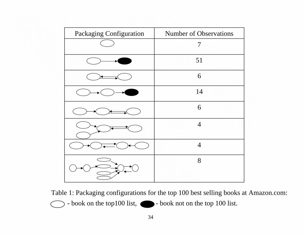
8

4

4

6

14

6

51

7Number of ObservationsPackaging Configuration

Table 1: Packaging configurations for the top 100 best selling books at Amazon.com:- book on the top100 list, - book not on the top 100 list.

34

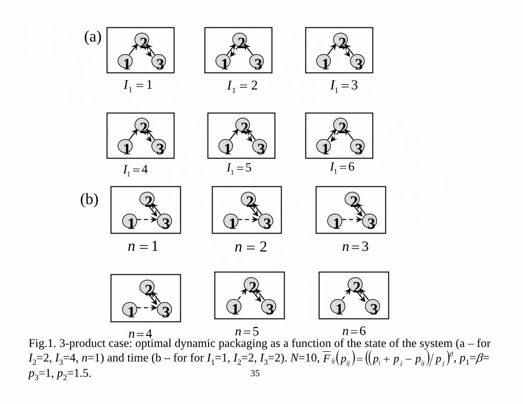
11 =I1

23 1

23

12

3 12

3

12

3

12

3

21 =I 31 =I

41 =I 51 =I 61 =I

1=n1

23

2=n 3=n

4=n 5=n 6=n

12

3 12

3

12

3 12

3 12

3

Fig.1. 3-product case: optimal dynamic packaging as a function of the state of the system (a – for I2=2, I3=4, n=1) and time (b – for for I1=1, I2=2, I3=2). N=10, , p1=β= p3=1, p2=1.5.

(a)

(b)

( ) ( )( )βjijjiijij pppppF −+=

35

36

( )21*12 ,, IInp

251 =I

11 =I

N-n=I2-1

n

Fig. 2. Optimal price for the “1-2” package as a function of the time index n for the Lost Sales model. Pricing functions and model parameters: (pij)=((pi+pj-pij)/pi)β, pij = pi , = pi + pj, β = 1, p1 = 1, p2 = 2, λ1 = λ2 = 0.4, Ι2 = 5.

ijF

ijp