Revenue management modelsfor hotel business

Dissertationzur Erlangung des akademischen GradesDoctor rerum politicarum (Dr. rer. pol.)

vorgelegt von

Master of Economics Andrei M. Bandalouskigeb. in Slonim

Erstgutachter: Prof. Dr. Erwin PeschZweitgutachter: Prof. Dr. Mikhail Y. Kovalyov

Tag der Einreichung: 05.03.2015

Fakultät III

Wirtschaftswissenschaften, Wirtschaftsinformatik

und Wirtschaftsrecht

Lehrstuhl für Wirtschaftsinformatik, Betriebliche

Anwendungs- und Entscheidungsunterstützungssysteme

Gutachter:Prof. Dr. Erwin PeschProf. Dr. Mikhail Y. Kovalyov

Datum der mündlichen Püfung: 30.04.2015Prüfer:Prof. Dr. Erwin PeschProf. Dr. Ulf LorenzProf. Dr. Mikhail Y. KovalyovPD. Dr. Sergei Chubanov

Gedruckt auf alterungsbeständigem holz- und säurefreiem Papier

I would like to dedicate this thesis to my grandmother Hanna Bandalouski

Declaration

I hereby declare that the thesis titled “Revenue management models for hotel business” is my

own work, except as specified in the text and Acknowledgements. The thesis has not been

submitted in whole or in part for consideration in any university for any other degree.

Andrei M. Bandalouski

2nd of March 2015

Acknowledgements

I would like to acknowledge Professor Mikhail Y. Kovalyov for the continuous support and

guidance throughout the whole common work, immense knowledge and experience and for

the sincere mentoring. I appreciate Professor Erwin Pesch for the supervision of the research,

for a high quality of advice he has provided and encouragement throughout procedures of

the defense process. I am thankful to Professor S. Armagan Tarim for the organization of the

research collaboration and contribution to production of the articles. Special thanks goes to

Dr. Natalija G. Egorova for her help with software programming. I also express gratitude to

Professor Emeritus Wayne Engel and David Haskell, who granted me an access to historical

database of hotel bookings, which helped me to illustrate the suggested revenue management

approach by considering the example of real hotel data.

Table of contents

List of figures vii

List of tables viii

1 Introduction 1

1.1 Motivation . . . . . . . . . . . . . . . . . . . . . . . . . . . . . . . . . . . 1

1.2 Setting Problem P-Pricing . . . . . . . . . . . . . . . . . . . . . . . . . . 5

1.3 Setting Problem P-Select . . . . . . . . . . . . . . . . . . . . . . . . . . . 6

1.4 Introductory survey of studies on interval scheduling . . . . . . . . . . . . 8

1.5 Outline of own results . . . . . . . . . . . . . . . . . . . . . . . . . . . . . 10

2 Survey of studies on dynamic pricing and revenue management 12

2.1 Hotel revenue management system . . . . . . . . . . . . . . . . . . . . . . 13

2.2 Processes of revenue management . . . . . . . . . . . . . . . . . . . . . . 17

2.3 Forecasting . . . . . . . . . . . . . . . . . . . . . . . . . . . . . . . . . . 18

2.4 Optimization . . . . . . . . . . . . . . . . . . . . . . . . . . . . . . . . . 22

2.5 Conclusion . . . . . . . . . . . . . . . . . . . . . . . . . . . . . . . . . . 34

3 Problem P-Pricing 35

3.1 General scheme . . . . . . . . . . . . . . . . . . . . . . . . . . . . . . . . 36

3.2 Demand disaggregation, input parameters and decision variables . . . . . . 38

3.3 Forecasting . . . . . . . . . . . . . . . . . . . . . . . . . . . . . . . . . . 41

3.4 Demand-price relations . . . . . . . . . . . . . . . . . . . . . . . . . . . . 46

Table of contents vi

3.5 Optimization . . . . . . . . . . . . . . . . . . . . . . . . . . . . . . . . . 48

3.6 Computer experiments . . . . . . . . . . . . . . . . . . . . . . . . . . . . 51

3.7 Conclusion . . . . . . . . . . . . . . . . . . . . . . . . . . . . . . . . . . 54

4 Survey of studies on fixed interval scheduling for HRM 55

4.1 The basic fixed interval scheduling problem . . . . . . . . . . . . . . . . . 55

4.2 Graph theory definitions . . . . . . . . . . . . . . . . . . . . . . . . . . . 58

4.3 Problem P1-HRM . . . . . . . . . . . . . . . . . . . . . . . . . . . . . . . 60

4.4 Problem P2-HRM . . . . . . . . . . . . . . . . . . . . . . . . . . . . . . . 62

4.5 Problem P3-HRM and problem P-HRM . . . . . . . . . . . . . . . . . . . 66

4.6 Conclusion . . . . . . . . . . . . . . . . . . . . . . . . . . . . . . . . . . 68

5 Problem P-Select 69

5.1 Simple variants of Problem P-Select . . . . . . . . . . . . . . . . . . . . . 69

5.2 A reduction to the maximum weight clique problem . . . . . . . . . . . . . 70

5.3 Solving problem MWC(P-Select) through enumeration of maximal cliques 71

5.4 Heuristic algorithms . . . . . . . . . . . . . . . . . . . . . . . . . . . . . . 77

5.5 Computer experiments . . . . . . . . . . . . . . . . . . . . . . . . . . . . 79

5.6 Conclusion . . . . . . . . . . . . . . . . . . . . . . . . . . . . . . . . . . 81

6 Conclusions 83

References 86

List of figures

2.1 Revenue management system of a hotel . . . . . . . . . . . . . . . . . . . 13

3.1 Processes interconnection . . . . . . . . . . . . . . . . . . . . . . . . . . . 38

4.1 Request intervals for two rooms and the corresponding P-Select-graph . . . 64

5.1 Digraph G(N1,D1) . . . . . . . . . . . . . . . . . . . . . . . . . . . . . . 76

List of tables

2.1 Forecasting methods . . . . . . . . . . . . . . . . . . . . . . . . . . . . . 21

2.2 Virtual nesting of seats . . . . . . . . . . . . . . . . . . . . . . . . . . . . 31

2.3 Equivalent notions . . . . . . . . . . . . . . . . . . . . . . . . . . . . . . 33

3.1 Forecasted numbers of check-ins . . . . . . . . . . . . . . . . . . . . . . . 45

3.2 Forecasted lengths of stay . . . . . . . . . . . . . . . . . . . . . . . . . . . 45

3.3 Comparison of revenues . . . . . . . . . . . . . . . . . . . . . . . . . . . 53

5.1 Quality of the solutions obtained by Heuristics G1, G2, and G3 . . . . . . . 80

5.2 Comparison of Heuristics G1, G2, and G3 with 2PA and Greedyα . . . . . 81

Chapter 1

Introduction

1.1 Motivation

Competition and macroeconomic changes stimulate hoteliers to find ways to improve busi-

nesses. Hotel Revenue Management (HRM) techniques evolve and their beneficial results

attract more and more hotel owners. Solutions of hotel revenue management approaches

support managers in decision-making and increase revenues, see, for example, Bandalouski

et al. (2015).

There are several popular definitions of the revenue management in the hotel terminology,

see Bandalouski et al. (2014). Haddad et al. (2008) define revenue management as a tool that

correlates supply of rooms with demand and maximizes income of a hotel by dividing its

customers into different categories based on their booking choices and the current capacity of

the hotel. Kimes and Wirtz (2003) define the term as employment of the information systems

and pricing strategies, which match orders with the corresponding free rooms over time.

Jauncey et al. (1995) consider revenue management as an integrated, continuous, systematic

approach for maximizing the income coming from the sale of rooms with variable prices,

based on the forecasted demand. Donaghy et al. (1995) follow approximately the same

concept, but also stress the importance of the market segmentation. They define revenue

management as a method of maximizing the revenue, which increases the net income of a

hotel through the correlation of the predicted number of available rooms with the predefined

1.1 Motivation 2

segments of the market at an optimal price. Jones and Hamilton (1992) argue that the revenue

management tries to maximize the room price when the demand exceeds the supply, and to

maximize the hotel capacity when the supply exceeds the demand, without falling in price

below the average cost. All the definitions point to the ability of the revenue management to

increase the income of a company without a direct control of costs. The essence of common

definitions is that the HRM is a tool to increase the income of a hotel by making appropriate

room prices and hotel capacity decisions.

Revenue management and dynamic pricing are the most popular intelligent decision

tools to increase profitability of various businesses, see Bandalouski et al. (2014). They first

appeared in the passenger air service in the late 1970’s. Their advantages were fully revealed

by American Airlines in 1985. There, the result of the first year of deployment of the revenue

management approaches led to the income increase by more than 14% and profit increase

by 48%, see Nguyen (2013). In the 1990’s, the hotel business has begun to adopt passenger

air service experience of revenue management by adjusting its principles, models and tools

for its own specificity. The implementation of the revenue management models in the hotel

business turned possible because hotel, transportation and other service businesses have the

following similar characteristics: 1) limited resources, such as rooms, passenger seats, rented

cars, entertainment tickets; 2) the products or services with a limited period of sale, whose

value deteriorates over time; 3) the ability to accept orders to be satisfied in the future; 4)

low per product or service costs and high fixed costs; 5) fluctuating demand for products or

services; 6) the ability to segment the market or customers, see Kimes (2004) and Casado

and Ferrer (2013). Many service companies possess these characteristics. That is why, in the

recent past, such companies which offer renting of convention centers, golf courses, cars,

traveling on cruise liners, as well as restaurants, shopping centers, etc., have begun to use

revenue management in their operations, see Maddah et al. (2010).

At present, theoretical knowledge, practical experience and application software are

well developed in the revenue management for airlines (McGill and van Ryzin (1999)).

Less attention is paid to the hospitality business. Researches in the latter area are rather

1.1 Motivation 3

fragmentary. There is a gap between the revenue management theory and its practice in

hotels.

There is an area in research of revenue management problems in which revenue optimiza-

tion is performed provided that the demand is given, it exceeds available resources and the

problem is to choose such demand requests that maximize revenue. Such a problem arises

in cottage or accommodation rental and hotel businesses. Landlords and real estate agents

collect booking requests during a certain period of time. In order to maximize revenue they

need to decide which booking request is to accept and which to reject. Hotel managers make

the same decisions due to periods of excessive demand, which occur during external events

or high season. Except accommodation rental business the problem arises in many decision

making situations such as assignment of transport devices to loading/unloading terminals in

ports, work planning of personnel in companies, bandwidth allocation of communications

channels, printed circuit board manufacturing, gene identification, and examining computer

memory structures. Keywords of this area research are “combinatorial auctions”, “interval

scheduling” and “cottage renting”.

Since the first practical success of the revenue management, an extensive research on this

subject has been conducted, see, for example, Kimes (2004), Bitran and Caldentey (2003),

Chiang et al. (2007), Elmaghraby and Keskinocak (2003), Weatherford and Bodily (1992).

Among existing literature reviews of revenue management in the hotel business, there are

some general systematizing studies (Kimes (2004), Jones and Hamilton (1992), Chiang et al.

(2007), Ivanov and Zhechev (2012)), as well as systematizing studies of the forecasting

component (Burger et al. (2001), Chen and Kachani (2007), Phumchusri and Mongkolkul

(2012)) and an optimization component (Bitran and Monschein (1995), Goldman et al.

(2002)).

Mission of the forecasting component of HRM approaches is to determine future demand

for the hotel rooms, see Bandalouski et al. (2014). The quality of approaches is highly

dependent on the forecast accuracy. Pölt (1998) calculated that, when using a revenue

management approach, reducing the forecast error by 20% leads to the 1% increase of the

income. Before setting a forecasting model, the following questions have to be answered:

1.1 Motivation 4

1) what to forecast; 2) which degree of aggregation of the forecasting objects to choose; 3)

to restrict or not to restrict the demand; 4) which historical period, called forecast base, to

use; 5) which forecasting horizon to choose; 6) which forecasting method to use; 7) which

accuracy is reasonable.

An optimization component of HRM approaches is intended to solve the problem of

maximizing the hotel revenue via identifying best prices or optimal allocation of limited

resources (seats in airplanes, rooms in hotels) or both of them. Taking into account different

types of rooms, price fares and durations of stay, this problem is not as simple as it seems.

Details of the optimization methods in the revenue management are given in Weatherford

(1998), McGill and van Ryzin (1999), Boyd and Bilegan (2003), Pak and Piersma (2002).

A rapid development of the information technologies, growth of the e-commerce and

the universal deployment of the Internet have led to the situation that, in the first decade of

the 21st century, the dynamic pricing tools have become an active component of the revenue

management approaches, see Feng and Gallego (1995), Dasu and Tong (2010), Anjos et al.

(2005) and Lin (2006). The main reasons for the increasing implementation of these tools

are the following: 1) digital data processing allows efficient collection and use of valuable

information about the demand and available inventory, prices of competitors, and processing

this information in real time; 2) costs of retyping price tags and informing customers about

the price changes have almost disappeared (Brynjolfsson and Smith (1999)), 3) customers

can easily follow the price changes.

Weatherford and Bodily (1992), McGill and van Ryzin (1999) provided general surveys

of the revenue management, including dynamic pricing as a part of it. Note that the term of

revenue management replaced the earlier concept of yield management, see Kimes (2004).

McGill and Van Ryzin mentioned the works of Gaimon (1988), Lau and Lau (1988) and

Weatherford (2001), where the price determination and the resource management problems

are combined. Gaimon attempted to consolidate price and capacity issues. Weatherford

considered the average value of a normally distributed demand as a linear function of the

price.

1.2 Setting Problem P-Pricing 5

Some researchers, for example, Boyd and Bilegan in Boyd and Bilegan (2003), tend to

separate dynamic pricing models from the revenue management models. However, they still

acknowledge their interrelation and similarity in certain cases such as the case of the one

room type.

1.2 Setting Problem P-Pricing

Analysis of the literature reveals that most studies on hotel revenue management concentrate

either on demand forecasting or on revenue optimization, subject to the given demand or its

probabilistic distribution, see recent review of Bandalouski et al. (2014). Researchers modify

existing forecasting methods and optimization models, invent new ones but rarely combine

them into a holistic practical revenue management approach. We suggest that studying a

combined problem and incorporating its solution into the real hotel revenue management

systems opens new theoretical problems, and fills the gap between theory and practice of the

hotel revenue management.

Consider such combined multi-product dynamic pricing problem for hotel revenue

management, which we denote as Problem P-Pricing. It is a dynamic and uncertain problem

of determining prices of rooms of different categories such that the total profit of room sales

based on the forecasted demand is maximized, assuming that the demand is price sensitive. A

typical example of a practical situation where Problem P-Pricing appears is the reservation of

hotel rooms via an Internet service, which immediately accepts a request if it can be satisfied.

Problem P-Pricing can be formulated as follows. There are rooms of several types and

uncertain demand of several categories, which specify room type, high or low season, time

before arrival, length of stay, etc. The demand is assumed to be price sensitive such that

fτ,c(pτ,c) = aτ,c − bc pτ,c, where, given category c and night τ , fτ,c is the corresponding

demand (number of occupied rooms of demand category c at night τ), pτ,c is the price, bc > 0

is the constant, called elasticity coefficient in the literature on demand-price relations, see

Houthakker and Taylor (1970), which show the responsiveness of the quantity demanded of

a hotel service to a change in its price, and aτ,c > 0 is a constant.

1.3 Setting Problem P-Select 6

Each unit of the demand implies a service cost. Historical values of the demand and price

values are given. The problem is to determine: 1) coefficients bc > 0 and aτ,c > 0, based on

the historical data, and 2) prices such that the total revenue minus the total service cost is

maximized over a given planning horizon, provided that the prices satisfy given lower and

upper bounds and a given linear order, and the room capacities are not exceeded.

Problem specific historical forecasting methods are used to predict values bc and aτ,c.

Then, these values are transferred to a mathematical programming problem with a concave

quadratic objective function and linear constraints, which aims at maximizing the total profit

of a hotel. Optimal prices for each category c and night τ of the planning horizon are the

solution of the Problem P-Pricing. Given optimal prices p∗τ,c, we can compute corresponding

demands aτ,c −bc p∗τ,c. These values are estimates of the hotel occupancy for each night of

the planning horizon and room type and they can be used for planning service activities.

There can be two hotel booking policies based on the solution of the Problem P-Pricing.

The first policy is to accept every incoming request and update solution after each booking.

The second policy is to accept as many requests from each category as determined by the

optimal demand values aτ,c −bc p∗τ,c. The excessive requests will be rejected. The efficiency

of the second policy strongly depends on the demand forecast quality.

An original software is being designed to solve Problem P-Pricing. The mathematical

programming problem is solved by a standard optimization software such as IBM (2014)

ILOG CPLEX.

1.3 Setting Problem P-Select

Consider another problem of hotel revenue optimization. Problem P-Select is a static and

deterministic problem of selecting a subset of room requests from a given set of room requests

such that the selected requests can be assigned to physically different rooms of the same type

or the same room in different time slots and the total value of these requests is maximized.

The setting of Problem P-Select is as follows. There are m rooms of the same type,

which are also denoted as unrelated parallel machines, and n requests, alternatively denoted

1.3 Setting Problem P-Select 7

as independent non-preemptive jobs, to stay in these rooms. A request j specifies a fixed

time interval I jl := (s jl,d jl], s jl < d jl , for each room, j = 1, . . . ,n, l = 1, . . . ,m. Each

request j can be either accepted by assigning it to exactly one time interval I jl , l = 1, . . . ,m,

or rejected. The former action brings value w jl and the latter action brings zero value.

w jl = ∑d jl−1t=s jl

ct,d jl−s jl , s jl < d jl, j = 1, . . . ,n, l = 1, . . . ,m, and ct,L is the room price for the

night between days t and t +1 depending on the length of stay L. For each room l, a set of

requests Nl is specified such that no request j ∈ Nl can be assigned to room l, l = 1, . . . ,m.

Furthermore, room unavailability intervals Uvl = (avl,bvl], avl < bvl, v = 1, . . . ,ul , are given

such that room l cannot be assigned any request within these intervals, l = 1, . . . ,m. Denote

Ul = U1l ∪ ·· · ∪Uul l , l = 1, . . . ,m. Note that Ul = /0, l = 1, . . . ,m, because rooms can be

occupied in some periods by earlier bookings.

A solution is characterized by the set of accepted requests and their assignments to the

rooms. A solution and the corresponding assignments are feasible if the following constraints

are satisfied: a) if request j is assigned to room l for processing within the interval I jl ,

then j ∈ Nl and I jl ∩Ul = /0, j = 1, . . . ,n, l = 1, . . . ,m; and b) time intervals of the requests

assigned to the same room do not overlap. The problem is to find a feasible solution that

maximizes the total value.

Observe that if I jl ∩Ul = /0, then request j cannot be assigned to room l. Therefore, all

such requests can be removed from the set Nl . Let us remove all such requests from each set

Nl. After this modification, the relation I jl ∩Ul = /0 is satisfied for j ∈ Nl , l = 1, . . . ,m. From

now on, we assume without loss of generality that there is no unavailability interval for each

room. In this case, there are at most 4mn numbers in the input of the Problem P-Select. They

are the request indices from the sets Nl , and the values w jl , s jl , and d jl , j ∈ Nl , l = 1, . . . ,m.

A typical example of a practical situation where problem P-Select appears is renting of

private apartments and cottages, when the owner collects requests during a certain period of

time and then decides which of them to accept. It also appears in hotel business in cases when

managers can not give immediate responds to requests but collect them during a certain period

of time and then accept or reject based on a revenue maximization criterion. For example,

such cases may occur during booking periods for world sporting events, when requests for

1.4 Introductory survey of studies on interval scheduling 8

rooms come much in advance and demand is usually exaggerated. These conditions allow

managers to consider requests during a certain period of time.

Problem P-Select is modeled as a Fixed Interval Scheduling Problem on parallel machines.

It is NP-hard in the strong sense. Its relation to the Maximum Weight Clique Problem of

graph theory is established. Optimal and heuristic solution approaches are developed based

on the properties of graphs and tested.

1.4 Introductory survey of studies on interval scheduling

Problem P-Select have been presented in Ng et al. (2014) and is a generalization of the

problem studied in Arkin and Silverberg (1987). The difference is that in the latter problem

w jl = w j, s jl = s j, and d jl = d j for each request j, and Ul = /0, l = 1, . . . ,m, i.e., the rooms

are of the same type and continuously available. We denote this problem as ISDI (Interval

Scheduling on Dedicated Identical parallel machines) and its special case where each room

can be assigned any request, i.e., Nl = {1, . . . ,n}, Ul = /0, l = 1, . . . ,m, as ISI (Interval

Scheduling on Identical parallel machines). Arkin and Silverberg prove that problem ISDI

is NP-hard in the strong sense for a variable number of rooms m and it is solvable in

O(mnm+1) time and space by a reduction to the problem of finding a longest path in a

specifically designed network with O(mnm+1) arcs. Arkin and Silverberg suggest several

solution approaches for problem ISI, the best of which can be implemented in O(n2 logn)

time. Bouzina and Emmons (1996) suggest improved algorithms for problem ISI and its

special case where all the request weights are unit. These algorithms run in O(mn logn) and

O(nmax{logn,m}) time, respectively. For the unit-weight case, Faigle and Nawijn (1995)

use the same algorithm as that of Bouzina and Emmons. They highlight that the algorithm is

an optimal on-line algorithm because it assigns a newly arrived request by using information

only about the requests that have arrived so far. In the considered on-line model, they assume

that a non-completed request can be rejected. The best existing (off-line) algorithm for

problem ISI with unit weights is due to Carlisle and Lloyd (1995). It runs in O(n logn) time.

1.4 Introductory survey of studies on interval scheduling 9

Carlisle and Lloyd also present an algorithm for the general problem ISI with the same time

complexity as that of Bouzina and Emmons.

Problem P-Select is polynomially reducible to the Weighted Job Interval Selection

Problem on One Machine with Arbitrary Weights (WJISP1) studied in Erlebach and Spieksma

(2003). In problem WJISP1, there is a single room and several request. A collection of time

intervals is associated with each request. Let N be the total number of intervals. The objective

is to select a maximum weight subset of the intervals such that (i) no two selected intervals

intersect and (ii) at most one interval is selected for each request. Given an instance of

Problem P-Select, the corresponding instance of problem WJISP1 can be obtained by shifting

each interval I jl to start (l −1)T time units later, l = 1, . . . ,m, where T is the length of the

planning horizon in the corresponding instance of Problem P-Select. Spieksma (1999) proves

that problem WJISP1 with unit weights is strongly NP-hard even if the length of each interval

is equal to 2 and at most two intervals intersect at each time instant. Furthermore, this problem

cannot have an Polynomial Time Approximation Scheme, unless P = N P . It follows from

his proof that these results also apply to Problem P-Select under the same conditions. Berman

and Dasgupta (2000) develop an O(n logn) time ρ-approximation algorithm with ρ = 1/2

for WJISP1, which delivers a solution with a value at least ρ times the value of an optimal

solution for any instance of this problem. This approximation result also applies to Problem

P-Select.

Recent studies of interval scheduling problems concentrate on on-line versions of the

interval scheduling problem, and heuristic and meta-heuristic solution approaches. Epstein

and Levin (2010) present on-line randomized algorithms for an on-line interval selection

problem and evaluate the competitive ratios of such algorithms. Eliiyi and Azizoglu (2011)

study a more constrained problem, in which the total number of requests assigned to each

room is limited. They suggest a filtered beam search algorithm and a heuristic that generates

and evaluates “promising” sets of selected requests.

1.5 Outline of own results 10

1.5 Outline of own results

The thesis consists of six chapters: Introduction, Survey of studies on dynamic pricing and

revenue management, P-Pricing dynamic approach, Survey of studies on interval scheduling,

Problem P-Select and Conclusion.

Chapter 2 gives basic concepts and a brief description of revenue management models

and decision tools in the hotel business. An overview of the relevant literature on dynamic

pricing, forecasting methods and optimization models is provided.

Chapter 3 describes a solution approach for Problem P-Pricing. Section 3.1 gives a

general scheme of our approach. Rational of demand disaggregation, the mechanism of its

disaggregation into categories, which are characterized by a set of demand parameters, and

input parameters for further mathematical analysis are discussed in Section 3.2. Forecasting

techniques are presented in Section 3.3. We modify Holt’s double exponential smoothing,

moving average and “the same day last year” historical forecasting methods to account for

disaggregated demand. Section 3.4 deals with the determination of demand-price relations.

It determines anticipated coefficients of category’s demand functions and links forecasting

and optimization stages of the approach. An optimization model is given in Section 3.5.

Optimization aims at maximizing the total profit of a hotel. Solution of the mathematical

programming problem with a concave quadratic objective function and linear constraints

gives optimal prices for each demand category. Computational experiments and its results

are described in Section 3.6.

Chapter 4 gives the detailed overview of existing models, results on computational

complexity and solution algorithms of interval scheduling. It describes the defining character-

istics of the fixed interval scheduling problem and its general formulation for hotel revenue

management. Relations to cognate problems in graph theory are provided.

Section 5.1 of Chapter 5 discusses some simple variants of Problem P-Select that can

be applied in practice. In Section 5.2 we reduce Problem P-Select to the problem of finding

a maximum weight clique in a specially constructed graph. We denote this problem as

MWC(P-Select) and the problem of finding a maximum weight clique in an arbitrary graph

as MWC. All the existing techniques for solving problem MWC can be used for solving

1.5 Outline of own results 11

Problem P-Select. Among these techniques there exist polynomial time algorithms for

specific graph classes. Furthermore, for some of these classes, there exist polynomial time

algorithms for recognizing the membership of an arbitrary graph in such a class. These

algorithms can be used to efficiently solve some instances of Problem P-Select. Section 5.3

describes a specific exact algorithm for problem MWC(P-Select) based on an enumeration of

the maximal cliques in graphs that describe time interval intersections of requests. While the

algorithm is not polynomial, it is efficient for some special cases or particular instances of

problem MWC(P-Select). Section 5.4 provides three polynomial time heuristic algorithms

for Problem P-Select. We report the results of computational experiments to compare the

performance of our and other existing heuristics for Problem P-Select in Section 5.5.

Chapter 6 concludes the thesis, gives suggestions for future research of various problems

related to P-Pricing and P-Select, and states perspectives for hotel revenue management

approaches.

Chapter 2

Survey of studies on dynamic pricing

and revenue management

Revenue management and dynamic pricing models are well explored in the field of passenger

air transportation. Literature reviews on dynamic pricing often refer to the results from this

business. Similarity of the sale conditions between hotel rooms and seats in the airplane

explains that some authors describe only the transition conditions of a model from one area

to another.

Our review considers studies of revenue management in the hotel business which have

been carried out since the late 1990’s mostly. We also touch research of revenue management

in other businesses which have direct implications for the hotel business.

This chapter is closely related to the paper Bandalouski et al. (2014). Section 2.1 rep-

resents hotel revenue management as a system, gives it general structure and surveys the

decision instruments applied in HRM. Section 2.2 describes general processes of revenue

management. Sections 2.3 and 2.4 provide detailed overviews of the research of the forecast-

ing and optimization processes respectively.

2.1 Hotel revenue management system 13

2.1 Hotel revenue management system

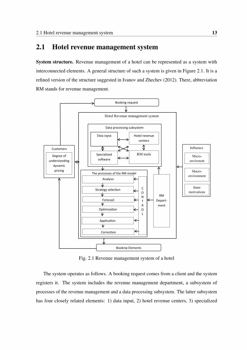
System structure. Revenue management of a hotel can be represented as a system with

interconnected elements. A general structure of such a system is given in Figure 2.1. It is a

refined version of the structure suggested in Ivanov and Zhechev (2012). There, abbreviation

RM stands for revenue management.

Booking request

Hotel Revenue management system

Data processing subsystem

Data input Hotel revenue centers

Specialized software

RM tools

The processes of the RM model RM

Depart-ment

Analysis

Strategy selection

Forecast

Optimization

Application

C ON T R O L

Booking Elements

Influence Micro-

environent

Macro- environment

Inner motivations

Customers

Degree of understanding

dynamic pricing

Correction

Fig. 2.1 Revenue management system of a hotel

The system operates as follows. A booking request comes from a client and the system

registers it. The system includes the revenue management department, a subsystem of

processes of the revenue management and a data processing subsystem. The latter subsystem

has four closely related elements: 1) data input, 2) hotel revenue centers, 3) specialized

2.1 Hotel revenue management system 14

software, and 4) revenue management tools. Input data contain all the information about

the booking request and, possibly, information about the customer. Specialized software

registers a booking request and begins its processing with a certain strategy. If the hotel has

only one revenue center, then it is responsible only for the basic income from the room sales.

If there are several revenue centers, then each of them is responsible for the corresponding

service: spa and fitness area, restaurant and bar, game room, and others. The subsystem of

processes treats a specific order and determines its status: the number and types of ordered

rooms, period of stay and price. The revenue management department, directly or indirectly,

approves the result of this treatment, and it goes back to the customer. The result and

the decision approach of handling the orders affect the customers perception of the hotel

pricing system and the hotel in general, and customers intention to deal with the hotel in the

future. The revenue management system is constantly influenced by the external and internal

environments.

Decision instruments. Choosing the right decision tool, by which the revenue manage-

ment system will maximize the hotel income, is very important. There exist many such tools.

Basically, they can be divided into price and non-price ones. Price based instruments include

price discrimination, cost barriers, dynamic pricing, guaranties of the lowest prices and other

tools directly affecting the price. Non-price instruments do not change prices directly, but

they are related to the resource management, control of overbooking, room availability and

the duration of stay. Both types of instruments are often used in practice simultaneously.

Non-price instruments. Pullman and Rogers (2010) examine resource management

tasks from a general perspective. They divide them into short term and strategic ones.

Strategic tasks are associated with a physical increase of the hotel capacity (number of

rooms) depending on the demand. Short term tasks deal with planning everyday occupancy,

check-in/check-out time and workforce timetabling.

The process of the overbooking control is based on the assumption that, for some reason,

a part of clients will not show up in the hotel. Therefore, hotels may sell more rooms than

they have, but it is important to plan the excess level. This topic was explored in Hadjinicola

2.1 Hotel revenue management system 15

and Panayi (1997), Ivanov (2007), Ivanov (2006), Koide and Ishii (2005), Netessine and

Shumsky (2002).

Less attention in the literature is paid to the control of the duration of stay. Usually, a

minimum number of nights to stay in the hotel is fixed. Such actions are being implemented

to protect the hotel from short stay orders in the periods of high demand and to increase the

length of stay in the periods of low demand. This topic was investigated in Kimes and Chase

(1998) and Vinod (2004).

Price instruments. The core of price instruments is price discrimination, which is based

on the price sensitivity of different groups of customers, such as tourists and business people,

see Kimes and Wirtz (2003), Hanks et al. (2002), Ng (2009). Due to the price discrimination,

the same room can be sold at different prices to the customers of different groups.

To avoid the transition of customers from high to low prices, hotels set up price barriers,

see Zhang and Bell (2010). Special conditions of room sale define these barriers. For

example, a hotel may sell rooms at given prices only for certain days of the week or for a

certain minimal duration of stay. It can keep a strict policy of cancellation or sell specific

rooms only to certain types of customers.

Sometimes hotels guarantee customers the lowest price, which is available on the market.

This means that, if a client in 24 hours will find another hotel with a room at a lower price,

they will equate the prices. This approach was explored in Carvell and Quan (2008) and

Demirciftci et al. (2010).

Dynamic pricing is the most widespread and developed intelligent pricing tool, see

Palmer and McMahon-Beattie (2008). Through it, a hotel offers prices which correlate with

the current level of the demand and occupancy, and respond to their changes. Dynamic

pricing can be used as a tool to compete for the maximal profit with firms offering the same

service (Rubel (2013), Sibdari and Pyke (2014)). Dynamic pricing models differ from the

optimization models of inventory management in that the former models perceive demand as

a function of variable price, while the latter models consider various given demand scenarios

with fixed prices, see Elmaghraby and Keskinocak (2003).

2.1 Hotel revenue management system 16

Price is one of the most effective variables of the business profit. By changing the price,

managers can encourage or restrict the demand in a short term, as well as regulate the on-hand

inventories (free rooms). While the demand depends on the price, the price is constrained

by the time in which the order is made, the existing demand level, the availability of the

rooms and other factors. Computer experiments conducted in Koenig and Meissner (2010)

revealed an advantage of dynamic pricing to list pricing. Sato and Sawaki (2013) considered

the case of duopoly when one of two competitors adopts a static pricing strategy and the

other competitor adopts a dynamic pricing. They showed cases in which dynamic pricing is

preferable.

Combining dynamic pricing with resource and inventory management. Many ex-

perts came to understanding that resource optimizing and inventory control decisions cannot

be separated from the pricing decisions and that the dynamic pricing tools must be a part of

the global revenue management system.

An opportunity to handle the forecasted demand by dynamic pricing tools as well as

optimization models of revenue management is the reason that the names of both methods

have become interchangeable, see Boyd and Bilegan (2003). Van Ryzin and Gallego (1997)

indicate the natural affinity between pricing and resource management models. If price is

treated as a variable, then it can be continuously monitored, and a decision to refuse an

order can be effectuated by sufficiently raising the price. The revenue management problems

through the prism of dynamic pricing were also studied in Ladany and Arbel (1991), Gallego

and van Ryzin (1994),van Ryzin and Gallego (1997), Feng and Gallego (1995) and You

(1999).

Integration of pricing and capacity allocation decisions have been carried out in Feng and

Xiao (2006a) and Feng and Xiao (2006b). Their continuous-time models combine price and

inventory decisions, and the pricing and capacity control policy is based on a sequence of

precalculated threshold time points that take into consideration the inventory, price and the

demand intensity. A set of thresholds is obtained by solving the Hamilton-Jacobi equation.

This model applies to maximizing revenues for a single time period. A similar approach has

been used in Shi et al. (2014) for determining the production level and selling price of one

2.2 Processes of revenue management 17

type of a product in a make-to-stock manufacturing system. Cao et al. (2012) extend studies

of continuous-time models by incorporating a discounting revenue criterion into them.

Classification of dynamic pricing models. There exist several classification schemes

for the dynamic pricing models. Bitran and Caldentey (2003) formulate a general problem of

maximizing the income of a company, which owns a limited, deteriorating in value set of

resources, and deals only with the price sensitive customers. For this problem, they suggest

using various dynamic pricing models, dividing them into deterministic and stochastic

ones. In each category, they study the cases of single and multiple types of products, and

consider solutions with one static price for the whole season and with several dynamic prices.

Elmaghraby and Keskinocak (2003) divide dynamic pricing models into categories based

on the following: 1) renewable or non-renewable resources; 2) dependent or independent

demand; 3) myopic or rational consumers.

Price constraints. It should be mentioned that a search for an optimal pricing strategy

often includes price constraints. Among the most common constraints are:

• choosing price from a given set, see Chatwin (2000), Feng and Gallego (2000), Feng

and Xiao (2000a), Feng and Xiao (2000b);

• upper limit on the number of price changes, Feng and Gallego (1995);

• a given shape of the price function: decreasing or increasing over time, special offers

on certain days, see Bitran and Mondschein (1997);

• price restrictions for a range of products;

• prices limited by costs.

2.2 Processes of revenue management

There exist different processes in revenue management. Tranter et al. (2008) describe eight

such processes: customer awareness, market segmentation, internal analysis, competitive

analysis, demand forecasting, analysis of distribution channels, dynamic pricing and inventory

2.3 Forecasting 18

control. Emeksiz et al. (2006) suggest five processes to describe a revenue management

system: preparation, supply and demand analysis, application of the revenue management

system, its evaluation, and monitoring and making changes to the system. Based on the

literature review and our experience in the hotel business, we suggest that five processes

– analysis, forecasting, optimization, control and adjustment – can be used to adequately

describe proper functioning of a HRM system.

Analysis includes processing the input data, the most important of which are the demand

and the information about the clients and the hotel resources.

Forecasting and optimization are the two most important and necessary components of

the whole system, see Cross (1997). At the transition from forecasting to optimization, there

is a connection of the future demand with the hotel capacities. It is important to have a low

forecast error, which makes the optimization model adequate. The choice of the forecasting

method depends of the demand behavior, and the choice of the optimization tool depends on

the truthfulness and accuracy of the input forecasted data and the computational complexity

of the optimization problem.

Control consists in monitoring the achievement of the main goal – maximization of

income – and in identifying errors and omissions of the modeling approach.

Adjustment aims at properly correcting the errors so that they do not appear in the future.

Below we will describe in detail the two main components - forecasting and optimization.

2.3 Forecasting

Demand forecasting. The main forecasting object in the hotel business is the demand, each

unit of which, called an order, a reservation or a booking, specifies the reservation date,

the arrival date, the room type and the duration of stay. It can be also associated with a

probability of cancellation. The reservations can be placed days, weeks or months before the

arrival date.

The nature of reservation cancellations is similar to the reservations, except for the two

important features: one can only cancel a confirmed order, and an order can be canceled

2.3 Forecasting 19

a given number of days before the arrival date. The difference between the number of

reservations and the number of cancellations is called net reservations.

The demand can be of different degree of aggregation – aggregated, partly aggregated

and completely disaggregated demand – and this degree implies using the corresponding

forecasting approach. The choice of the aggregation degree depends on the type of the

available input data. The completely aggregated forecasting approach generates the overall

future demand of the hotel, which is further divided between room categories based on the

given ratios between them. The completely disaggregated approach generates future demand

for each category, and then, if it is needed, the data is combined. Weatherford et al. (2001)

argue that the fully disaggregated forecast usually gives better results than partly aggregated

or aggregated forecast.

The demand in a hotel business has a high degree of seasonality. If a small forecast base

period is used, for example, eight - twelve weeks, then the seasonality cannot be properly

addressed, and if the period is large, then the seasonality can be better addressed, but, in

this case, a proper base period has to be chosen. A large forecast base period can make the

forecast not responsive enough.

The period for which the forecast is built is called forecasting horizon. A forecasting

horizon can be long-term and short-term. The long-term horizon usually covers one year.

The short-term horizon usually varies from one day to three months.

Forecasting methods. Lee (1990) identifies three types of forecasting methods: his-

torical bookings, advanced bookings and combined. Historical bookings methods include

exponential smoothing, moving average, copying demand from the same day of the previous

year, linear regression and autoregressive method (AR), methods of Box-Jenkins ARMA

and ARIMA. Exponential smoothing is applied to time series data to forecast smoothed

data. The time series data themselves are a sequence of units of demand. While in the

moving average the past observations are weighted equally, exponential smoothing assigns

exponentially decreasing weights over time. The autoregressive method specifies that the

forecasted demand depends linearly on its own previous values. ARMA methods combine

autoregressive and the moving average methods, and it applies only to stationary time series.

2.3 Forecasting 20

ARIMA methods extend ARMA methods for the non-stationary time series. The historical

bookings methods use only data from a certain period in the past, such as the total number of

arrivals in a particular day. We observed that the early studies often concentrated on simple

methods, while the later studies deal with the more sophisticated methods such as ARIMA.

The results of the forecasting competition accomplished by Makridakis et al. (1982) show

that the sophisticated methods such as ARIMA do not perform statistically better than the

simple methods in computer experiments with real data.

Advanced bookings methods, also called pickup methods, consider future as well as al-

ready committed reservations. There are additive and multiplicative versions of the advanced

bookings methods. The additive version assumes that the number of already committed reser-

vations at a certain day before the arrival is independent of the final number of reservations

for the arrival day. In contrast, the multiplicative version assumes that the number of already

committed reservations influences future reservations. In the additive bookings method, the

number of reservations for a certain day T , forecasted at the current day T − k, is obtained

as the sum of the number of already committed reservations for day T and the sum of k

numbers ct , t = 0,1, . . . ,k, where ct is the number of reservations made for the day T − t − i

, i = 0,1, . . . ,L, t days before the arrival and averaged over i = 1, . . . ,L, and T − k−L is

the first day of the historical period. In the multiplicative method, the forecasted number

of reservations for day T forecasted at the current day T − k is obtained as the product of

the number of already committed reservations for day T and of k numbers pt , t = 0,1, . . . ,k,

where pt is the average ratio of number of reservations made for day T − t −u to the number

of reservations at day T − t−u+1, u = 1, . . . ,L, and T −k−L is the first day of the historical

period.

Combined methods use the best features of the historical bookings and advanced bookings

methods and combine them, either by weighted averaging or regression methods. The method

of using neural networks also belongs to this group. Fildes and Ord (2002) and Ben-Akiva

(1987) believe that the combined methods provide the most accurate forecast results. A short

overview of the forecasting methods is given in Table 2.1.

2.3 Forecasting 21

Table 2.1 Forecasting methods

Historicalbookings

Exponential smoothing

Burger et al. (2001), Chen and Kachani (2007),Rajopadhye et al. (2001), Weatherford andKimes (2003), Yüksel (2007), Phumchusri andMongkolkul (2012)

Moving averageBurger et al. (2001), Weatherford and Kimes(2003), Yüksel (2007)

AR, ARMA, ARIMABurger et al. (2001), Lim and Chan (2011), Limet al. (2009), Yüksel (2007)

Advancedbookings

AdditiveChen and Kachani (2007), Weatherford andKimes (2003)

Multiplicative Weatherford and Kimes (2003)

CombinedRegressive

Burger et al. (2001), Chen and Kachani (2007),Weatherford and Kimes (2003)

Weighted average Chen and Kachani (2007)

Forecast accuracy. Making a proper choice of the forecast method is very important.

Most often, accuracy is the main criterion for this choice. There are several measures to

assess the accuracy of the forecast. An assessment based on the Mean Absolute Error (MAE)

is the most simple and applicable method. Absolute deviations of the forecasted past values

from the real past values can be calculated for each day of a historical period. The average

of these deviations is the MAE. The smaller the MAE value the better is the forecast. The

Mean Percentage Error (MPE), the Mean Absolute Percentage Error (MAPE), the Root

Mean Square Deviation (RMSD) and other measures are also popular, see Phumchusri and

Mongkolkul (2012). Armstrong and Collopy (1992) carried out a fairly complete evaluation

of error measures with respect to the reliability, construct validity, sensitivity to small changes,

protection against outliers and relationship to decision making.

The effectiveness of the forecasting methods can be evaluated in different ways. Weath-

erford and Kimes (2003) used real historical data of Choice Hotels and Marriott Hotels to

compare the effectiveness of the forecasting methods. They deduced that the exponential

smoothing, the moving average and the method of selecting already committed orders provide

the most accurate forecasts. Based on the results reported in the literature, Fildes and Ord

(2002) deduced that combined methods give better accuracy compared to historical and

2.4 Optimization 22

progressive methods. Zakhary et al. (2008) observed in their computer experiments with

simulated data that the additive version of advanced method gives more accurate results

than the multiplicative version. Schnaars (1984) noted that, when the input data is highly

variable, the method of transferring the demand from the same day in the past is superior to

other popular methods. Despite some differences in the appraisals, all researchers agree that

different methods should be applied to different data types, determined by season, type of

customers and other characteristics.

Some researchers propose to incorporate experience and knowledge of experts into the

forecasting methods, and combine them with the mathematical instruments. This direction

of research is popular nowadays. Several authors state that the hotel managers are able to

give a very accurate forecast for the two or three week period, see, for example, Rajopadhye

et al. (2001). The human assessment is particularly useful in the presence of external events

that can affect the future demand.

2.4 Optimization

The first optimization models were developed for passenger air transportation. Then, because

of similarity of mathematical models and the scope, they moved into the hotel business.

We will review the existing revenue optimization models by using the air transportation

terminology. Occasionally, we will provide hotel interpretation of the results.

Optimization techniques of air transportation revenue management are most often pub-

lished under the name of seat inventory control. Seat inventory control (optimization) tech-

niques can be partitioned into two major groups - class control and network seat inventory

control methods.

Class control methods are based on stochastic principles which incorporate demand

distributions and reservation and cancellation probabilities. They can be divided into static

and dynamic solution methods. Static methods determine the best allocation of seats once,

before sales start, based on the demand forecast and capacity information available at this

moment. It is common way to use static methods repeatedly over the booking period. Dy-

2.4 Optimization 23

namic methods allocate seats in each class over time, depending on the real-time information

about reservations and seats availability. Every time the dynamic system gets a request, it

decides on the acceptance or rejection of the reservation and the price.

Network seat inventory control methods include deterministic and stochastic mathemati-

cal programming models, virtual nesting and bid price methods and simulation and dynamic

systems approaches. Below we will review these techniques in more detail.

Seat inventory control. Seat inventory control models form the core of the optimization

models in the air passenger transportation, see Chiang et al. (2007). They aim at maximizing

the revenue through the right allocation of the limited number of seats to each of the fare

classes. The seat requests occur over time before the flight departure. The seat request

specifies a route and a specific fare class. Once an optimal allocation of the seats to the fare

classes is computed based on the forecasted demand, it is used to develop a booking control

policy, which specifies the rules of accepting or rejecting incoming seat requests. The nature

of the customer requests is stochastic, and the customers can pay different prices. Prices

for each class in each route segment are given and the airline offers them to the customers.

Naturally, at a certain point in time it is more profitable to reject a low fare request for a seat

in order to be able to accept a higher one later for the same seat.

The main methods of seat inventory control are: 1) single leg seat inventory control

(class control), which optimizes the number of seats sold for each flight leg separately, and 2)

Origin-Destination and Fare (ODF) class control, also called network seat inventory control,

which optimizes the number of seats sold for the entire network of flight legs at all fare

classes. The flight leg is the direct flight between two points without a stop. Each route in the

network consists of one or more flight legs. If a flight is going from Minsk to Istanbul and

then to Ankara, then Minsk-Istanbul and Istanbul-Ankara are the legs and Minsk-Ankara is

the route. The network refers to the complete network of the flight legs offered by the airline.

ODF control operates with triples (origin, destination, fare class).

Fare classes. Airlines create a set of services known as classes which vary not only

because of the separate location of seats in the airplane. For example, assume that an airline

sells seats in four classes – A, B, C and D. Each class is associated with its price. Class A

2.4 Optimization 24

is associated with the highest price and deluxe meal, and it has no restriction on the ticket

exchange or refund. Class D price is the lowest, no meal is included, and the tickets cannot be

exchanged or refunded. Classes B and C have reasonable prices, regular meal is included, and

there are some restrictions on the ticket exchange and refund. Different customer segments

prefer different fare classes.

Class control. For each leg the class control method determines a certain amount of

seats that can be sold in each class. The amount of seats in each class can be different for

each leg. For the entire route which comprises several legs, the seats of the same passenger

must be of the same class for all legs. For example, a passenger can book tickets of class A

on a route comprising leg 1 and leg 2 only if A class tickets are available on both legs. Let

us consider the case of two legs POINT1-POINT2 and POINT2-POINT3 and assume that

each of them has only one empty seat. There are only two customers willing to buy tickets.

One passenger is willing to pay 70$ for class A in the leg POINT1-POINT2 and the other

passenger is willing to pay 210$ for class A in the route of two legs POINT1-POINT2 and

POINT2-POINT3. In the class control method, seats are available only if the leg and the

class are both available at the same time. It is also impossible to block the 70$ request for

the class A seat while the 210$ class A seat is still open for sale. The class control method

does not control such cases and therefore loses opportunities to increase income.

Static solutions. Littlewood (1972) was the first to propose static solutions with two

classes. He suggested closing the class of a low price and transfer remaining seats to the

higher class when the expected income from the sale of the next seat in this class is lower

than the expected income from the sale of the same seat in the higher class. Belobaba (1987)

offered a so-called nested approach for multiple classes, which is a modification of the

approach of Littlewood (1972). The new approach has been termed the Expected Marginal

Seat Revenue approach (EMSRa). It produces so called nested protection levels. Such levels

are defined as upper bounds on the number of seats allocated to the fare classes. Optimal

policies of this approach were independently presented in Curry (1990) and Wollmer (1992).

Curry suggested that the distribution of the demand is continuous, while Wollmer supposed

that it is discrete. Brumelle and McGill (1993) suggested another approach, named EMSRb,

2.4 Optimization 25

which considers both continuous and discrete distribution of the demand. It is based on the

idea of equating the marginal revenues in the various fare classes. The authors state that the

EMSRb approach provides greater protection for higher valued fare classes than the EMSRa

approach. The nested approach is commonly used to solve class control problems.

A multistage static stochastic programming model for airlines business was presented

in Williams (1999). Since stochastic programming models have become nowadays a very

popular decision tool in many applications, including hotel business, let us describe this

model in detail. We will use the hotel terminology because the problem in Williams (1999)

admits an evident hotel business interpretation.

The hotel owns rooms of three types i = 1,2,3. Types 1 and 2, and 2 and 3 are called

adjacent to one another. The booking horizon is divided into T time periods and the current

time period is t = 0. In each time period t = 0,1, . . . ,T −1 room reservations are made for

time period T . In time period T , there are ni rooms of type i, and ri percent of rooms of this

type can be transformed into the rooms of the adjacent types. The price of a room of type i to

be used in time period T , which is booked and paid in time period t, 0 ≤ t ≤ T −1, can take

one of the values ct,i,1, . . . ,ct,i,Ot , where Ot is the number of price options in time period t.

The model in Williams (1999) decides the room prices and the number of rooms of each type

for each time period in the planning horizon.

The demand values are the numbers of rooms of each type which will be booked in

the current time period and they will be used in time period T . It is assumed that the

demand is uncertain and that its values depend on the price. Assume that the forecast gives

St demand scenarios for time period t. While the demand values depend on the price, it

is assumed that the demand scenarios do not depend on the price. They depend on the

external economical, political and social factors. The demand scenarios in time period t are

assumed to be independent events that form a full system of events in this time period. Let

the probability of scenario s in time period t, 1 ≤ s ≤ St , be pt,s. We have ∑Sts=1 pt,s = 1.

The model suggests the construction of a scenario tree. The tree has T +1 levels denoted

t = 0,1, . . . ,T , each consisting of a number of nodes. Each node (t,s) of level t is associated

with a demand scenario s in time period t, t = 0,1, . . . ,T , s = 1, . . . ,St . Level 0 consists of the

2.4 Optimization 26

artificial node (0,0), where 0 is an artificial scenario that happens with probability 1 in time

period 0. It is assumed that, for each node (t+1,b), there is exactly one arc ((t,a),(t+1,b)),

which means that the scenario b in time period t + 1 happens after the scenario a in time

period t, t = 0,1, . . . ,T −1. If there is an arc ((t,a),(t +1,b)), then node (t,a) is called a

parent of node v = (t +1,b) and denoted as prnt(v).

Each node (t,st) of level t is associated with a unique scenario path v = ((0,0),(1,s1),

(2,s2), . . . ,(t,st)) ending in this node, sτ ∈ {1, . . . ,Sτ}, τ = 1, . . . , t. Since we are in time

period 0, the probability that the scenario path v = ((0,0),(1,s1),(2,s2), . . . ,(t,st)) will lead

to the demand scenario st in time period t is equal to Pv = ∏tτ=1 pτ,sτ

. Let Vt denote the set of

all scenario paths ending in the nodes of level t, t = 1, . . . ,T . Due to the tree-like precedence

relations, |Vt |= St .

Assume that, for each scenario path v ∈ Vt , the demand in time period t for rooms of

type i and price o to be used in time period T , denoted as dv,i,o, is known or forecasted.

There are the following decision variables:

1. xv,i,o – the number of rooms of type i for time period T to be sold in time period t at

price o assuming that the scenario path v ∈Vt has been realized, 0 ≤ t ≤ T −1;

2. yv,i,o – auxiliary indicator variable; yv,i,o = 1 if xv,i,o > 0 and yv,i,o = 0 if xv,i,o = 0,

v ∈Vt , 0 ≤ t ≤ T −1;

3. zv,i – auxiliary variable that expresses the total number of rooms of type i for time

period T to be sold along the scenario path v, v ∈Vt , 0 ≤ t ≤ T .

2.4 Optimization 27

The deterministic model of the problem can be formulated as follows.

maxT−1

∑t=0

∑v∈Vt

Ot

∑o=1

Pvct,i,oxv,i,o, (2.4.1.1)

s.t.Ot

∑o=1

yv,i,o = 1, v ∈Vt ; i = 1,2,3; t = 0, . . . ,T −1, (2.4.1.2)

xv,i,o ≤ dv,i,oyv,i,o, v ∈Vt ; i = 1,2,3; o = 1, . . . ,Ot , t = 0, . . . ,T −1, (2.4.1.3)

zv,i =O1

∑o=1

x0,i,o, v ∈V1; i = 1,2,3, (2.4.1.4)

zv,i = zprnt(v),i,o +Ot

∑o=1

xprnt(v),i,o, v ∈Vt ; prnt(v) ∈Vt−1; i = 1,2,3; t = 2, . . . ,T,

(2.4.1.5)

zv,1 ≤ (n1 + ⌊r2n2

100⌋), v ∈VT , (2.4.1.6)

zv,2 ≤ (n2 + ⌊r1n1 + r3n3

100⌋), v ∈VT , (2.4.1.7)

zv,3 ≤ (n3 + ⌊r2n2

100⌋), v ∈VT , (2.4.1.8)

zv,1 + zv,2 ≤ (n1 +n2 + ⌊r3n3

100⌋), v ∈VT , (2.4.1.9)

zv,1 + zv,3 ≤ (n1 +n3 + ⌊r2n2

100⌋), v ∈VT , (2.4.1.10)

zv,1 + zv,2 + zv,3 ≤ n1 +n2 +n3, v ∈VT , (2.4.1.11)

xv,i,o ∈ Z+, v ∈Vt ; i = 1,2,3; o = 1, . . . ,Ot ; t = 0, . . . ,T −1, (2.4.1.12)

yv,i,o ∈ {0,1}, v ∈Vt ; i = 1,2,3; o = 1, . . . ,Ot ; t = 0, . . . ,T −1, (2.4.1.13)

zv,i ∈ Z+, v ∈Vt ; i = 1,2,3; o = 1, . . . ,Ot ; t = 0, . . . ,T. (2.4.1.14)

The objective function (2.4.1.1) is the total expected income from selling rooms in time

periods t = 0,1, . . . ,T −1 for time period T . Equations (2.4.1.2) guarantee that in any time

period only one price option will be chosen for each room type. Relations (2.4.1.3) ensure

that for any scenario path and any price option the number of rooms sold for each of the three

room types does not exceed the corresponding demand. Equations (2.4.1.4) and (2.4.1.5)

represent recursive calculation of values of variables z via values of variables x. Inequalities

2.4 Optimization 28

(2.4.1.6)-(2.4.1.8) ensures that the total number of rooms of type i to be sold in time period

T does not exceed the existing number of rooms of this type plus transformed rooms from

the adjacent type(’s). Inequality (2.4.1.9) ensures that the sum of the total number of rooms

of types 1 and 2 to be sold in time period T does not exceed the existing number of rooms

of these types plus transformed rooms from the type 3. Inequality (2.4.1.10) ensures that

the sum of the total number of rooms of types 2 and 3 to be sold in time period T does not

exceed the existing number of rooms of these types plus transformed rooms from the type 2.

Inequality (2.4.1.11) ensures that the sum of the total number of rooms of all types i to be

sold in time period T does not exceed the sum of existing number of rooms of these types.

Quantities of transformed rooms of each of the type can be determined from zv,1, zv,2, zv,3

and n1, n2 and n3 values.

Dynamic solutions. In the discrete time dynamic programming model in Lee and

Hersh (1993) demand for each class is modeled by an inhomogeneous Poisson process of a

Markovian type in such a way that, at any given time t, the booking requests before time t do

not affect the decision to be made at time t. The decision rule is that a booking request is

accepted if its price exceeds the opportunity costs of the seat. Authors define opportunity

costs as the expected marginal value of the seat at time t. Kleywegt and Papastavrou (1998)

showed that the class control problem can be formulated as a dynamic stochastic knapsack

problem. Subramanian et al. (1999) added accounting for cancellations to the model proposed

by Lee and Hersh.

Network seat inventory control. Comparing with the class control method, the network

seat inventory control method is more efficient for reservations which include transfers,

because it optimizes the entire network of flights in all fare classes offered by the airline.

One of the techniques of this method is to distribute the expected income of the entire route

in proportion to its legs and then to use the class control method for each leg.

2.4 Optimization 29

Glover et al. (1982), Talluri and van Ryzin (1999) and many others formulate the problem

of network seat inventory control as the following deterministic mathematical programming

problem.

max ∑i∈I

rixi, (2.4.2.1)

s.t. ∑i∈I(l)

xi ≤ cl, l ∈ L, (2.4.2.2)

xi ≤ di, i ∈ I, (2.4.2.3)

xi ≥ 0, i ∈ I. (2.4.2.4)

where I is the set of all pairs (route, class), ri is the price of one seat for the (route, class)

pair i, variable xi is the number of orders for the pair i, L is the set of legs in the network, I(l),

I(l)⊂ I, is the set of pairs (route, class) for the leg l, cl is the capacity of the leg l, and di is

the expectation of the number of orders for the pair i. The problem is to determine numbers

of orders which maximize the total income ∑i∈I rixi.

Let x∗ denote an optimal solution of the problem (2.4.2.1)-(2.4.2.4). A booking control

policy is generated by setting upper bound x∗i on the number of orders for each pair i, i ∈ I.

As it is mentioned by many authors, e.g., Pak and Piersma (2002) and de Boer et al.

(2002), the optimal revenue value of (2.4.2.1)-(2.4.2.4) is an upper bound for the same

stochastic problem.

The problem (2.4.2.1)-(2.4.2.4) assumes that there is a single flight in a single time

window for each route in the network. Multiple flights of the same route can be considered

by making copies of this route.

2.4 Optimization 30

A stochastic version of the model (2.4.2.1)-(2.4.2.4) was suggested in Wollmer (1986).

This model, called Expected Marginal Revenue (EMR) model, is the following.

max ∑i∈I

c0i

∑k=1

riPDi≥kXi,k, (2.4.3.1)

s.t. ∑i∈I(l)

c0i

∑k=1

Xi,k ≤ cl, l ∈ L, (2.4.3.2)

Xi,k ∈ {0,1}, i ∈ I, k = 1,2, . . . ,c0i , (2.4.3.3)

where Di is the demand for the (route, class) pair i, PDi≥k is the probability that this demand

will be at least k, and c0i = max{cl | i ∈ I(l), l ∈ L} is the largest number of seats available

along all legs of the pair i. Decision variable Xi,k is equal to 1 if at least k seats are reserved

for the pair i, and it is equal to 0 otherwise. The value of riPDi≥k represents the expected

marginal revenue of allocating an additional k-th seat to the pair i.

A more sophisticated model of similar type that addresses service product upgrades is

suggested in Steinhardt and Gönsch (2012).

General stochastic network models, which are based on Markov decision processes and

several types of approximations, are offered in van Ryzin and Talluri (2003). Meissner and

Strauss (2012) incorporated customer choice into these models, in which a probability of

selecting a certain product by the arriving customer is given. A customized application

of Markov decision processes to the problem of determining rental rates in the apartment

lease industry is suggested in Chen et al. (2014). Özkan et al. (2013) formulate a Markov

decision process for situations in which demand depends on the current external environment,

representing economic, financial, social or other factors that affect customer behavior.

Virtual nesting and bid price methods. The most frequently used approaches in the

network seat inventory control are the virtual nesting and the bid price method. The virtual

nesting approach is similar to the class control method, but it eliminates the major inconve-

nience of the latter method by creating “virtual buckets” of seats based on the value rather

2.4 Optimization 31

than on the class. The approach creates value based virtual buckets on each leg, and then

requests for each leg in each pair (route, class) to be assigned to these virtual buckets.

Consider the example of two legs and the two passengers from the paragraph Class

control. Two virtual buckets are created in this case: Bucket 1 is for high value requests, and

Bucket 2 is for low value requests, see Table 2.2. Seats are made available in Bucket 1 on

both legs. To block a low value request and make a high value request eligible, the method

will assign the 70$ Class A request on the leg POINT1-POINT2 to Bucket 2 and the 210$

Class A request on the legs POINT1-POINT2 and POINT1-POINT2 to Bucket 1.

Note that, if there are multiple fare requests, the process of assigning them to the buckets

is not trivial. There are several approaches to assign different fare requests to the buckets,

see Williamson (1992) and de Boer et al. (2002).

Table 2.2 Virtual nesting of seats

Buckets/LegsPOINT1-POINT2,

number of seatsPOINT2-POINT3,

number of seatsBucket 1 (high value) 1 1Bucket 2 (low value) 0 0

The bid price method is similar to virtual nesting but it avoids complications with

assigning requests for pairs (route, class). The bid price is associated with the shadow price

and the displacement/opportunity cost of reducing the capacity of the leg by one seat, see

Williamson (1992). A shadow price is linked to each leg in the network and it represents

a marginal loss from reducing the capacity of this leg by one seat. The bid price (value,

opportunity cost of selling one seat) of a pair (route, class) in the network is equal to the sum

of the shadow prices over the legs comprising the route. A class for a route is opened for sale

if the price associated with this pair (route, class) exceeds its bid price. Otherwise, the class

is closed. An advantage of the bid price method is that it takes into account the remaining

capacity and open/closed pair (route, class) status only. Once a class is opened, there are no

limits on the number of accepted requests. In order to control the selling process, the bid

prices are refreshed periodically. Thus, some classes are closed and some classes are opened.

2.4 Optimization 32

The bid price method was explored in Williamson (1992), Wei (1997), Talluri and van Ryzin

(1998).

Simulation and dynamic approaches. Bertsimas and de Boer (2005) presented a

simulation based approach for the network seat inventory control problem. Their approach is a

combination of the deterministic linear programming and approximate dynamic programming.

It considers the expected revenue function as a function of the booking limits. The linear

programming model finds initial optimal values of those booking limits. Then the approach

improves solutions by considering the stochastic nature of the demand and employing virtual

nesting. The booking period is divided into small time periods, and the booking process

is simulated for the current time period. The booking control policy is formed only for

the current period. Revenue is calculated as the sum of the current period revenue and the

estimated revenue of the future periods, which depends on the remaining capacity.

A full dynamic solution of the network seat inventory control problem was first obtained

in Chen et al. (1998). They formulated the problem as a Markov decision problem and used

a linear programming model for the calculation of the objective function. The objective

function depends on the time until departure and the remaining capacity of the flights. The

customer requests are assumed to be independent of each other and Markovian. In order to

accept or reject a request, it is decided whether its price exceeds opportunity costs or not.

The method does an off-line approximation of the objective function but the booking policy

is implemented on-line. A similar approach is also suggested in Cooper and de Mello (2003).

Similarity of air transportation and hotel businesses. Optimization models and meth-

ods are almost the same for airlines and hotels. For an example, consider a situation that the

hotel can transform any room to be of any type, the number of rooms can change over time,

no client can change the room type during the entire stay. For this situation, the equivalent

notions in both businesses are given in Table 2.3.

Because of these relations, the linear programming model (2.4.2.1)-(2.4.2.4) can be used

to maximize the total income of the hotel.

The class control method can be interpreted and used for the hotel business too. In the

hotel terminology it can be called “room type control” method. The method establishes

2.4 Optimization 33

Table 2.3 Equivalent notions

Air transportation Hotel businessleg nightroute period of stayclass room typecapacity of leg l number of rooms for night lexpected number of orders forthe pair (route, class)

expected number of bookings for the pair (periodof stay, room type)

price of one seat for the pair(route, class)

price of one night for the pair (period of stay,room type)

availability of room types for each date in the planning horizon. A guest can order a room

of a certain type if it is available for sale for each date of the stay. Similar to the class

control method, the “room type control” method cannot examine reservations by the length

of stay. Therefore, reservations for a night or two occupy rooms and do not let the system

to accept the reservations with longer length of stay, which leads to the ineffective usage of

the resources. An analogue of the virtual nesting method associates different combinations

of the triple “arrival date - length of stay - room type” with the different buckets of room

requests for each night. The buckets differ by prices of room types. A room is sold if the

corresponding room type is present in the same bucket during the entire period of stay. An

analogue of the bid price method determines the bid price for every night. A room is sold if

the total payment for the corresponding stay exceeds the sum of the bid prices of the nights

in the entire stay period.

In a recent review, Ivanov and Zhechev (2012) observed that stochastic programming

(Goldman et al. (2002), Lai and Ng (2005), Liu et al. (2006), Liu et al. (2008)) and simulation

methods (Baker and Collier (2003), Rajopadhye et al. (2001), Zakhary et al. (2011)) prevail

among the optimization tools. Deterministic linear programming methods (Goldman et al.

(2002), Liu et al. (2008)), integer programming methods (Bertsimas and Shioda (2003)),

dynamic programming methods (Badinelli (2000), Bertsimas and Shioda (2003)) and fuzzy

goal programming methods (Padhi and Aggarwal (2011)) received less attention, but there is

a growing interest in them. The bid price method (Baker and Collier (2003)) is poorly used

in the hotel business.

2.5 Conclusion 34

2.5 Conclusion

In this chapter we provided a survey of the results for the dynamic pricing, hotel revenue

management and their components forecasting and optimization. In Section 2.3 we discussed

what has to be forecasted, described main forecasting methods and measures to asses accuracy

of the forecast. In Section 2.4, we reviewed seat inventory control models, gave equivalent

notions of air transportation and hotel business and interpreted airlines seat inventory control

models in terms of the hotel revenue management.

This survey revealed that there is a lack of studies on combined revenue management

problem, which integrate forecasting and optimization problems of HRM approaches. Study-

ing the combined problem and incorporating its solution approaches into the real revenue

management systems will open new theoretical problems.

Chapter 3

Problem P-Pricing

In this chapter we describe a solution approach for a multi-product dynamic pricing problem

for hotel revenue management (HRM), denoted as Problem P-Pricing. The approach is

illustrated on the data of a real hotel, which we denote as H. The approach takes into

consideration suggestions for future research made in Chapter 2 and includes determination

of input parameters for the succeeding mathematical analysis, disaggregation of the demand

into several categories, demand forecasting, simulation of demand-price relations, and a

mathematical programming model for price optimization. Demand forecast, simulation of

demand-price relations and determination of optimal prices are made separately for each

category and each day of the planning horizon. Demand is assumed to be elastic, more

specifically, it is assumed to be a linear decreasing function of the price. Prices are variables

in the mathematical programming model, whose criterion is to maximize the total hotel

revenue in the given time period, subject to the limited resources and upper and lower bounds

on the prices. The objective function is quadratic as it is a result of multiplying the prices

and the corresponding elastic demand values. Revenue maximization in each category leads

to the revenue maximization of the whole hotel.

We accept the following assumptions: 1) disaggregation of the demand into categories

leads to more accurate forecasting and optimization results, 2) the demand of different

categories does not correlate with each other and 3) the demand is elastic and depends only

on the price.

3.1 General scheme 36

Results of this chapter have been taken from the paper Bandalouski et al. (2015). Section

3.1 gives a general scheme of the solution approach Problem P-Pricing. Section 3.2 discusses

the rational of demand disaggregation, the mechanism of disaggregation into categories

and input parameters for further mathematical analysis. Section 3.3 presents forecasting

techniques. Section 3.4 deals with the determination of demand-price relations. An optimiza-

tion model is given in Section 3.5. Computational experiments and results are described in

Section 3.6.

3.1 General scheme

A rapid development of information technologies and e-commerce has supported employing

dynamic pricing approaches in the hotels and the research interest to this field. The fact

that the absolute majority of reservations come from Internet makes it easy to simulate

future demand in all categories, dynamically calculate and offer appropriate prices, and

automatically relate each incoming reservation with the appropriate category.

Our dynamic pricing approach also takes advantage of the recent information technologies.

Its main stages are given below.

1. Modification of a booking database of a hotel to the required format, which includes

such fields as the room type, the selling price, the check-in and check-out dates and

the date of reservation.

2. Determination of the following input parameters and decision variables:

(a) parameters that define demand categories;

(b) lower and upper bounds on price in each category and the corresponding reference

price;

(c) operational cost for each room type;

(d) planning horizon.

3. Input of parameters into the model.

3.1 General scheme 37

4. Forecasting, which includes

(a) formation of historical periods of time series of the numbers of realized check-ins

for each category;

(b) formation of historical periods of time series of lengths of stay associated with

each check-in in each category;

(c) forecast of the number of check-ins for each demand category and each night in

the planning horizon;

(d) forecast of the lengths of stay associated with each arrival in each demand

category and night in the planning horizon;

(e) arithmetic calculation of the number of occupied rooms for each demand category

and night in the planning horizon.

5. Determination of demand-price relations which includes

(a) calculation of the slope of the linear demand function for each category;

(b) calculation of the constant in the demand function for each category.

6. Optimization to determine an optimal price for each category and each night in the

planning horizon.

7. Output of the following results:

(a) optimal price for each category and for each night in the planning horizon;

(b) the anticipated number of rooms occupied in each category and each night of the

planning horizon.

Steps 4-7 are applied repeatedly after every registered booking. A graphical representation

of our approach is given in Figure 3.1.

Let us now describe our dynamic pricing approach in more detail.

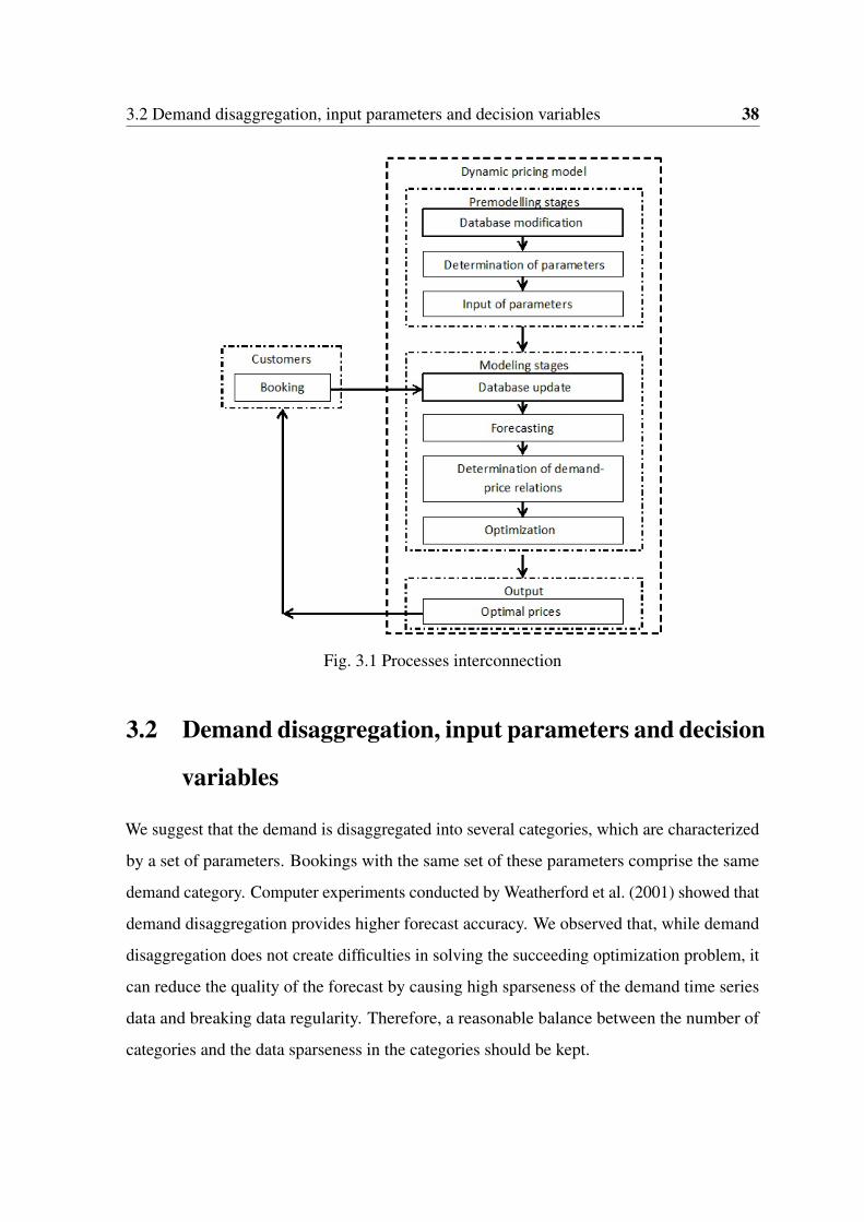
3.2 Demand disaggregation, input parameters and decision variables 38

Fig. 3.1 Processes interconnection

3.2 Demand disaggregation, input parameters and decision

variables

We suggest that the demand is disaggregated into several categories, which are characterized

by a set of parameters. Bookings with the same set of these parameters comprise the same

demand category. Computer experiments conducted by Weatherford et al. (2001) showed that

demand disaggregation provides higher forecast accuracy. We observed that, while demand

disaggregation does not create difficulties in solving the succeeding optimization problem, it

can reduce the quality of the forecast by causing high sparseness of the demand time series

data and breaking data regularity. Therefore, a reasonable balance between the number of

categories and the data sparseness in the categories should be kept.

3.2 Demand disaggregation, input parameters and decision variables 39

We will illustrate our approach by considering the example hotel H. For this hotel,

historical data of daily bookings is available for 2009-2012 years. We divide the demand of

hotel H into categories according to the following parameters: 1) type of the season denoted

as Season, 2) day of the week (Day), 3) length of stay (Length), 4) length of the time period

between the time of reservation and the check-in time (Before), and 5) fare class (Fare).

For hotel H, we distinguish two seasons: low season (Low) includes January–March

and November, and high season (High) includes the rest of the year. Days of the week are

characterized as week days (Mon-Thu) that include Monday to Thursday, and weekends

(Fri-Sun) that include Friday to Sunday. Demand of the same season type and day of the

week does not have seasonal and weekly fluctuations. By introducing parameters Season

and Day we move away from the need to “clean up” the data from seasonality at the forecast

stage.

We assume that the length of stay can be of two classes: less than or equal to 7 days (7−)

and more than 7 days (8+). The length of the time period between reservation and check-in

can be less than or equal to 7 days (7−), 8-30 days (8−30) and more than 30 days (31+).

The approach does not consider spot demand, that is, check-ins without a reservation. We

also define five fare classes: economy class (E), premium economy class (E+), business class

(B), premium business class (B+) and suite (S).

The result of the above classification is that each reservation is assigned to one of the

120 demand categories. The value 120 is obtained by multiplying numbers of values of

the category parameters, i.e., 120 = 2×2×2×3×5. Demand categories are denoted as c,

c = 1, . . . ,120. Demand category c is represented as follows:

c = (Season = X ,Day = Y,Length = Z,Be f ore =V,Fare =W ),

where X ∈{Low,High}, Y ∈{Mon−T hu,Fri−Sun}, Z ∈{7−,8+}, V ∈{7−,8−30,31+},

W ∈ {E,E+,B,B+,S}. For example, dc = (Season = High,Day = Fri− Sun,Length =

7−,Be f ore = 7−,Fare = B). Note that a check-in date of a reservation uniquely defines

type of the season and day of the week.

3.2 Demand disaggregation, input parameters and decision variables 40

The other input parameters for our revenue management approach are the planning

horizon, the room operational cost for each room type, the lower and upper bounds on the

price values in the demand categories and the reference price for each demand category. The

planning horizon is the period of time in the future for each day of which, starting from today,

optimal prices have to be determined. The room operational cost is the per day cost applied if

the room is in use. We require that the room price is not lower than the room operational cost.

The lower and upper bounds on the price values define the range in which the category price

may vary from manager’s perspective. Reference price or base price is the actual competitive

price for a room in the corresponding demand category which a manager has in mind.

The decision variables are prices for rooms in each demand category and each night of

the planning horizon.

There is an alternative either using lower and upper bounds on the price values in the

demand categories or a reference price for each demand category. If the decision maker

prefers the bounds on the price values in the demand categories then the reference price is

calculated as the average of these bounds. If the decision maker prefers the reference price,

which can be the last actual price in this demand category, then the lower and upper bounds

on the price values are the result of 50% deviation from the reference price. This alternative

in the input is the result of managers’ practice to work with the reference price or with the

price bounds.

To avoid entering price bounds or a reference price for each of the 120 categories manually,

managers are asked to set the price bounds/reference prices only for one category of each

room type, and then set the percentage deviation from this sample category for each value of

demand category parameters. This sample category has the highest price within the subset of

categories of one room type. For the hotel H, rooms are sold at the highest price in following

categories (Season=High,Day=Fri−Sun,Length= 7−,Be f ore= 7−,Fare=W ), where

W ∈ {E,E+,B,B+,S}. The price bounds/reference prices for rooms of categories with

parameters Season=Low, Day=Mon-Thu, Length=8+, Before=8-30 and Before=31+ will

be automatically decreased by a predetermined percentage, for example, by 15%, 8%, 8%,

3.3 Forecasting 41

8% and 15%, respectively. It is the responsibility of hotel managers to define and enter these

deviation values.

3.3 Forecasting

It is very important to choose a forecasting method which guarantees appropriate forecast

accuracy. The choice of the forecasting method strongly depends on the past reservation data

and the specificity of the entire HRM approach. In the literature, three major types of the

demand forecasting methods have been studied: historical, advanced and combined, see Lee

(1990) and Ivanov and Zhechev (2012). Disaggregation of the demand into categories may

cause an excessive data sparseness. Advanced and combined methods aim at monitoring and

maintaining regularities in sparse time series. However they are sensitive to the historical

input data, which affects their quality. Historical bookings methods do not include specific

tools to account for data regularities but they are not so sensitive to the input data and provide

stable and sufficiently accurate forecast results either for sparse or well saturated time series

(Makridakis et al. (1982), Schnaars (1984), Weatherford and Kimes (2003)). We employ

historical bookings forecasting methods because they are simple and effective with respect to

the demand disaggregation.

Demand forecasting starts with building two historical time series for each demand

category and day: 1) the number of realized check-ins and 2) the length of stay associated

with each check-in. Then, the forecasted numbers of future check-ins and their lengths of

stay are linked together in order to calculate the predicted number of occupied rooms in each

demand category and night in the planning horizon. These numbers are obtained by means of

arithmetic manipulations with the forecasted check-ins and lengths of stay. The succeeding

stages of our HRM approach use the number of occupied rooms for each category and day.

The length of the planning horizon varies from 1 day to 12 months. The same forecasting

method cannot give accurate results for short-term and long-term forecasting horizons. The

same observation holds with respect to the data sparseness, which depends on the level of

demand disaggregation. We consider demand data of each category as sparse if there were

3.3 Forecasting 42

no check-ins for at least one of the days of the demand time series in the historical period.

For forecasting periods up to three months, we either modify Holt’s double exponential

smoothing (M-Holt) or modify moving average (M-Moving). This alternative arises due

to the density condition of disaggregated historical data. Sparse data leads to inaccurate

estimates of the smoothing coefficients of level and trend and, consequently, to an error in

the M-Holt forecasting method. Therefore, M-Moving is applied to sparse data. Since the

accuracy of the demand time series extrapolation decreases with the extension of the planning

horizon, we modify “same day last year” (M-Same) forecasting for long-term periods of

three months or more. All three forecasting methods are modified by us in order to improve

forecast accuracy in the specific environment of our HRM approach.

Let us give details of the forecasting methods. First note that the length of the historical

period is method specific. Given a demand category, denote the realized value of the number

of check-ins in a past day i as si, i = 1, . . . , t, where t is the last day of the historical period,

and denote the number of forecasted check-ins in a future day i as si, i = t + 1, . . . , t +T ,

where T is the length of the planning horizon. We assume that check-ins are indexed

1, . . . ,q,q+1, . . . ,q+Q, where 1 is the first (oldest) check-in of the historical period, q is

the last check-in of the historical period and Q is the forecasted number of check-ins in the

planning horizon. We have Q = ∑Tm=1 st+m.

We will describe forecasting methods on the example of the number of check-ins.

Modified Holt’s Double exponential smoothing (M-Holt). Holt’s double exponential

smoothing forecasting method is an extension of the simple exponential smoothing method,

see Gardner (2006), Rajopadhye et al. (2001). The advantage of Holt’s method is that,

besides the smoothed value of the series, it is able to capture medium-term trend. The trend

represents the direction in which the series is moving and reflects both internal effects of

changes in the hotel as well as external, which affect businesses in the region. The method

3.3 Forecasting 43

consists of a forecast equation and two smoothing equations:

st+m = lt +mrt , m = 1, . . . ,T, (3.3.1)

li = αsi +(1−α)(li−1 + ri−1), i = 2,3, . . . , t (3.3.2)

ri = γ(li − li−1)+(1− γ)ri−1, i = 2,3, . . . , t (3.3.3)

where li is an estimate of the level of the series at time i, ri is an estimate of the trend of the

series at time i and initial values of l1 and r1 are to be specified. α is a smoothing coefficient

for the level, 0 ≤ α ≤ 1, and γ is a smoothing coefficient for the trend, 0 ≤ γ ≤ 1.

The equation (3.3.1) shows that an m-step-ahead forecast is equal to the estimated level

at day t plus m times the estimated trend value at day t. The equation (3.3.2) shows that li is

a weighted average of observation si and the within-historical-period one-step-ahead forecast

for time i given by li−1 + ri−1. The trend equation (3.3.3) shows that ri is a weighted average

of li − li−1 and the previous estimate of the trend ri−1.

Optimal values for coefficients α and γ are estimated from the historical period. Coeffi-

cients are estimated by minimizing the mean square error (MSE). The within-historical-period

one-step-ahead forecast errors are specified as ei = si − si, i = 1, . . . , t, and MSE is specified

as MSE = ∑ti=1 e2

it . To calculate si, si = li−1 + ri−1, i = 1 . . . t, initial values of level and trend

can be specified as l1 = s1 and r1 =(s2−s1)+(s3−s2)+(s4−s3)

3 and initial values of coefficients α

and γ take arbitrary values within the interval [0,1].

In order to increase the accuracy of the forecast we have modified Holt’s double exponen-

tial smoothing method. Note that the original method can output fractional parts of values

of the demand, whose rounding can substantially distort the forecast results. To account for

the contribution of the fractional values of check-in time series we suggest to summarize

them starting from the first day of the planning horizon t + 1. As soon as the sum of the

fractional parts of the numbers of forecasted check-ins exceeds 1, an extra check-in unit is

generated. This unit is randomly added to one of the corresponding days. Therefore, no

forecasted demand is lost, which is essential for the disaggregated demand.

3.3 Forecasting 44

The length of the historical period affects accuracy of the M-Holt forecasting method. It

depends on the specific data of the hotel and varies from one month to one year. Experiments

conducted on the historical data of the hotel H suggested to set three months as the length of

the historical period.

Modified Moving average (M-Moving). The modified moving average method is

applied to sparse time series. We use it for short-term and medium-term planning horizons

with up to three months length. Moving average is simple but gives reliable results for sparse

historical data. Forecasting of values of time series for day t +1 is calculated by averaging

N, 1 ≤ N ≤ t, previous observations of the series by the following formula:

st+1 =1N

t

∑i=t−N+1

si.

The method suggests that st+m = st+1, m = 2,3, . . . ,T .

The criterion for choosing the optimal number of observations to average is the smallest

forecasting error. Computer experiments on the real historical data of hotel H have shown

that the minimum forecasting error is attained for N = 8.

Our modification of the moving average method concerns fractional values, similar to

that in the M-Holt method.

Modified method “the same day last year” (M-Same). In the forecasting method “the

same day last year”, the forecasted value of time series for the demand category in day t +1

is the assigned number of check-ins of the corresponding category at the same day of the

previous year.

To increase accuracy and add dynamics to forecasting method “the same day last year”

we suggest to modify it as follows. Let us forecast the number of check-ins for a day t +1.

Without loss of generality, let this day be a Friday. The method M-Same takes the number

of check-ins of the same day in the last year but adds to it an average value of deviations of

that value from check-in numbers of all Fridays in the last month. If there were 23 check-ins

on Friday of week 48 in year 2014 and the check-ins numbers on Fridays of weeks 47, 46,

3.3 Forecasting 45

45 and 44 in year 2015 were 25, 26, 23 and 24, respectively, then the forecasted number of

check-ins for Friday of week 48 in year 2015 would be 24,5 = 23+ 2+3+0+14 .

The above mentioned forecasting methods are employed to forecast the number of check-

ins for each demand category and night in the planning period, as well as the length of stay

associated with each check-in. These forecasted values are then used to calculate future

demand, that is, daily occupancy of the hotel, assuming that the price is fixed to be the

reference price.

Examples of forecasted numbers of check-ins for a demand category with Day = Fri−

Sun and forecasted lengths of stay associated with each check-in for the same category

are presented in Tables 3.1 and 3.2, respectively. It is assumed that check-ins are indexed

n = 1,2, . . ..

Table 3.1 Forecasted numbers of check-ins

Date Number of Check-incheck-ins indices

31.10.2014 0 -01.11.2014 3 54, 55, 5602.11.2014 0 -07.11.2014 0 -08.11.2014 0 -09.11.2014 1 5714.11.2015 0 -15.11.2015 2 58, 5916.11.2015 0 -

Table 3.2 Forecasted lengths of stay

Date Check-in Length ofindex stay

01.11.2014 54 201.11.2014 55 201.11.2014 56 209.11.2014 57 115.11.2014 58 215.11.2014 59 2

3.4 Demand-price relations 46

Note that the forecast of the lengths of stay will be done implicitly via the forecast of

check-ins if there is a separate demand category for each possible length of stay.

Some reservations made in the past can be canceled in the future before their check-ins.

In order to account for this situation, we calculate the probability of cancellation for each

demand category and assign a random number between 0 and 1 to each realized reservation.

If this random number is less than or equal to the corresponding probability of cancellation,

then the reservation is not counted in the future. For a given demand category, the ratio

between the number of canceled reservations and the total number of reservations in the

historical period for this category is taken as the probability of cancellation. Reservations

that have been made and decided to be counted in the future reduce the number of rooms

available during the corresponding period of stay.

Forecast results are intermediate. Forecasting gives a single point on the plot of the

demand-price relation for each category and day of the planning horizon. This point is

determined by the reference price and the forecasted demand. We assume that the demand is

a linear non-increasing function of the price.

3.4 Demand-price relations

Slope of the demand function. Consider an arbitrary demand category c and night τ . We

restrictively assume that the demand for this category and night is a linear function fτ,c of the

price pτ,c for this night and category: fτ,c(pτ,c) = aτ,c −bc pτ,c, where bc > 0 is the category

dependent slope of the demand function, which is also called elasticity coefficient in the

demand-price studies, see Marshal (1890), and aτ,c > 0 is a constant. Note that demand for

the hotel service products, which are room bookings, is price sensitive, contrary such goods

as inferior quality staple foods or luxury products, and therefore, the demand functions fτ,c

are non-increasing.

The elasticity coefficient for the demand category c is determined by a simple linear

regression approach. A maximal data set of historical data of the category is employed to fit

a straight line through the set of data points in such a way that makes the sum of squared

3.4 Demand-price relations 47

residuals of the simple linear regression model as small as possible. It is important to employ

all historical data available in order to get more realistic estimate of the slope of the demand

function. Explanatory variable of the regression function is the room price adjusted for

inflation, and dependent variable is the number of rooms sold for this price. Below we

will show how to adjust price for inflation. The fitted line represents the historical demand

function, and its slope determines the elasticity coefficient bc. The elasticity coefficient tends

to change only in a long term under the influence of external political and economic factors.

Therefore, calculated from the historical data, it does not depend on τ and it may be applied

to all nights in the planning horizon within the same category. Contrarily, the constant aτ,c of

the demand function fτ,c depends both on the demand category c and the day τ .

Before calculating elasticity coefficient bc, historical prices are adjusted for inflation as

follows:

Pa =Ph

1+RIx,

where Pa is a price adjusted for inflation, Ph is a historical price without adjustment for

inflation and RIx is the rate of inflation (RI) in the considered month x. It is calculated as

RIx =CPIx−CPI0

CPI0, where CPIx is the Consumer Price Index (CPI) for the considered month

and CPI0 is the CPI for the basic month, which is the latest month of the historical period. In

the USA, CPI’s are published by the Bureau of Labor Statistics of the Department of Labor

U.S. (2014).

Excessive sparseness of the data of some categories and the influence of unpredicted

factors may cause negative values of the elasticity coefficients bc. Since the demand function

fτ,c is assumed to be non-increasing, negative coefficients bc are considered as deviations

from the law. In such a case bc is set to zero.

Constant aτ,c. We suggest that the constant aτ,c is calculated as aτ,c = zτ,c+bc p0c , where

p0c is the reference price for the category c and zτ,c is the forecasted number of occupied

rooms for this category in day τ .

3.5 Optimization 48

3.5 Optimization

The optimization model aims at maximizing the total profit of a hotel. Input data for the

model are the defined parameters aτ,c and bc for each demand function fτ,c, the lower and

upper bounds on the price values of each category c, the room operational cost for each room

type and the number of available rooms of each type in each day τ . Maximization of the total

profit of a hotel is gained via solving the following constrained mathematical programming

problem.

maxk

∑c=1

t+T

∑τ=t+1

(aτ,c −bc pτ,c)(pτ,c −hc)−Wk

∑c=1

t+T

∑τ=t+1

yτ,c, (3.5.1)

subject to

Lτ,c ≤ pτ,c, τ = t +1, . . . , t +T, c = 1, . . . ,k, (3.5.2)

pτ,c ≤Uτ,c + yτ,c, τ = t +1, . . . , t +T, c = 1, . . . ,k, (3.5.3)

aτ,c ≥ bc pτ,c, τ = t +1, . . . , t +T, c = 1, . . . ,k, (3.5.4)

pτ,c ≥ hc, τ = t +1, . . . , t +T, c = 1, . . . ,k, (3.5.5)

∑c∈M j

(aτ,c −bc pτ,c)≤ Rτ, j, τ = t +1, . . . , t +T, j = 1, . . . ,5, (3.5.6)

pτ,c1 ≤ pτ,c2 , c1 ∈ M1, c2 ∈ M2, τ = t +1, . . . , t +T, (3.5.7)

pτ,c2 ≤ pτ,c3 , c2 ∈ M2, c3 ∈ M3, τ = t +1, . . . , t +T, (3.5.8)

pτ,c3 ≤ pτ,c4 , c3 ∈ M3, c4 ∈ M4, τ = t +1, . . . , t +T, (3.5.9)

pτ,c4 ≤ pτ,c5 , c4 ∈ M4, c5 ∈ M5, τ = t +1, . . . , t +T, (3.5.10)

pτ,c ≥ 0, yτ,c ≥ 0, ∀ τ, c. (3.5.11)

where the variables are pτ,c and yτ,c, and the given input parameters are the following.

• [t +1, t +T ] – the planning horizon,

• Lτ,c – the lower bound on the price pτ,c,

• Uτ,c – the upper bound on the price pτ,c,

3.5 Optimization 49

• hc – the operational cost of a room in category c,

• Rτ, j – the number of rooms of type j available in day τ ,

• yτ,c – the auxiliary variable that allows price upper bounds to be violated, when these

bounds make the feasible domain empty,

• W – a sufficiently large number that is greater than the optimal value of the problem in

which all variables y are equal to zero (price upper bounds are not violated). For exam-

ple, W can be set as the sum of largest values of the functions (aτ,c−bc pτ,c)(pτ,c−hc)

with respect to the variables pτ,c for all τ and c and the only constraints pτ,c ≥ hc and

aτ,c ≥ bc pτ,c. By this choice of W , if there exists a feasible solution with yτ,c = 0 for

all τ and c, then such a solution will always be optimal,

• M j – the set of all categories that include room type j. We assume that the sets M j are

numbered in non-decreasing order of the room prices.

Objective function (3.5.1) includes total profit with the positive sign and price upper

bounds extension costs with the negative sign. We stress, that the extension costs are artificial

and do not contribute to the total profit. Relations (3.5.2) and (3.5.3) address price lower

and upper bounds, respectively. Note that the positive values of the variables y indicate

how much hotel managers may exceed the highest prices in cases of excessive demand in

order to balance the current levels of demand and supply. Potential to exaggerate prices

helps managers not to reject customers. Constraints (3.5.4) guarantee that the demand takes

non-negative values only. Relations (3.5.5) require that the room price is not less than the

room operational cost. Constraints (3.5.6) ensure that the sum of the requested number of

rooms of each type in different categories in day τ does not exceed the number of available

rooms of type j in this day. Constraints (3.5.7)–(3.5.10) secure the price hierarchy of room

types.

Our optimization model does not allow overbooking. It may happen that the forecasted

demand for the reference price exceeds the corresponding room capacity. Then the model

3.5 Optimization 50

will try to increase the price in order to decrease demand in order to satisfy the capacity

constraint.

The problem (3.5.1)-(3.5.11) is a mathematical programming problem with a concave

quadratic objective function and linear constraints. The objective function is concave because

it is the sum of concave quadratic functions of one variable. The problem can be solved by

a standard optimization software, for example, IBM (2014) ILOG CPLEX Optimization

Studio Version 12.6.

Note that the problem (3.5.1)-(3.5.11) can be decomposed into T subproblems. Each

subproblem considers one day τ , τ = t +1, . . . , t +T . An optimal solution of the original

problem is determined by the optimal solutions of the subproblems.

Optimization is the last stage of our approach for the hotel revenue management. Solution

of the problem (3.5.1)-(3.5.11) specifies optimal price p∗τ,c for each category c in each day τ

of the planning horizon and optimal values of the slack variables y∗τ,c. Data for the considered

hotel H includes 5 room types, 2 values of the parameter Length and 3 values of the parameter

Before. Therefore, the cardinality of the daily set of optimal prices for the hotel H is 30.

If the period of stay of an incoming reservation starts in one category (low season or

weekday) and ends in another category (high season or weekend), then the period of stay is

divided into several parts, each of a unique category, and the corresponding price is calculated

for each part.

Given optimal prices p∗τ,c, we can compute corresponding demands aτ,c −bc p∗τ,c. These

values are estimates of the hotel occupancy for each day and room type and they can be used

for planning service activities.

A solution of the problem (3.5.1–3.5.11) can be analyzed and approved or modified by

the decision makers. An approved solution is made accessible to the potential guests of the

hotel.

There can be two booking policies based on the solution of the problem. The first policy

is to accept every incoming request and update the solution after each booking. The second

policy is to accept as many requests from each category as determined by the optimal demand

values aτ,c −bc p∗τ,c. The excessive requests will be rejected. The efficiency of the second

3.6 Computer experiments 51

policy strongly depends on the demand forecast quality. Irrespectively of the booking policy,

we suggest a price update after every realized booking, because every booking decreases

the number of available rooms. We also suggest to set up several planning horizons with

different lengths, for example for 1, 7, 31, 90, 180 and 360 days, and update solutions for all

of them simultaneously. Accuracy of the forecast and, therefore, solution quality decreases

as the length of the planning horizon increases. Therefore, solutions for the shorter planning

horizon should be more accurate.

3.6 Computer experiments

In order to evaluate the efficiency of our dynamic pricing approach we conducted a computer

experiment to compare actual revenue of the example hotel H in the past period with the

modeled potential revenue generated by our approach for the same past period, which we

call comparison period, subject to an assumption that the demand is price sensitive.

Since we have used confidential input data, we have multiplied all numbers by a certain

same coefficient and rounded them.

In the experiment, room operational cost, hc, was set to 50 for all room types. 10 rooms of

the hotel H were considered. Reference prices of the most valuable categories of room types E,

E+, B, B+ and S were set to 139, 149, 159, 175 and 189, respectively. Percentage deviations

for categories with parameters Season=Low, Day=Mon-Thu, Length=8+, Before=8-30

and Before=30+ were set to 20%, 10%, 10%, 10% and 15%, respectively. The approach

employed the M-Moving forecasting method.

A past period of 90 days was considered. It was divided by a fixed day t into two periods:

initial historical period of 30 days t −29, t −28, . . . , t, and initial planning horizon of 60 days

t +1, t +2, . . . , t +60. 14 days t +31, t +32, . . . , t +44 were used as the comparison period.

The reason for choosing these days is that no booking with parameter Before=31+ made in

day t or later can have a check-in at day t +30 or earlier.

The experiment was run on a PC with Intel Core i5 2.4×2 GHz processor and 4 GB of

RAM under MS Windows 8.1 Pro (64 bit). IBM (2014) ILOG CPLEX Optimization Studio

3.6 Computer experiments 52

Version 12.6 has been used to solve the mathematical programming problem (3.5.1)-(3.5.11).

To account different tendencies of demand changing in the planning horizon compared to

the historical period, three types of scenarios were considered. Past periods of 90 days were

different for each of the scenario. In the steady scenario, the daily number of check-ins in the

historical period does not much differ from the daily number of check-ins in the planning

horizon. Low-grow and high-grow scenarios are characterized by low and high growth,

respectively, of daily check-ins in the planning horizon in comparison with the same values

in the historical period.

In each scenario, the algorithm ran for τ = t, t +1, . . . , t +13. In each run, the solution

method was applied for historical periods τ − 29,τ − 28, . . . ,τ and the planning horizon

τ +1,τ +2, . . . ,τ +60. Modeled revenue was calculated for day τ +31 of the comparison

period. Numerical results are shown in Table 3.3.

The experiment demonstrated that our dynamic pricing approach increases the average

revenue of the hotel in comparison with the static pricing strategy. Moreover, due to the

fact that the cost structure of the hotel business is characterized by high fixed and low

variable costs, the ability of the approach to increase revenue brings even a relatively greater

contribution to profit than to revenue. Added revenue contributes to overall profit greater if

variable costs are lower.

Zero values of actual revenue at days of the comparison periods were due to that no

rooms had been sold at those days. Differences of the modeled revenue over and under the

actual revenue had been caused by the modeled optimal prices and the corresponding number

of rooms would be sold for these prices. Our dynamic pricing approach showed the highest

revenue growth in the steady scenario, in which demand values at the planning horizon did

not differ much from the past values. High accuracy of the demand forecast in this scenario

significantly contributed to the total revenue gained. Speed of the future demand change

decreased forecast accuracy and added revenue but still saved the margin positive.

3.6 Computer experiments 53

T abl

e3.

3C

ompa

riso

nof

reve

nues

Low

-gro

wsc

enar

ioH

igh-

grow

scen

ario

Stea

dysc

enar

io

#

Dat

esof

com

-pa

riso

npe

riod

Act

ual

reve

nue

Mod

eled

reve

nue

#

Dat

esof

com

-pa

riso

npe

riod

Act

ual

reve

nue

Mod

eled

reve

nue

#

Dat

esof

com

-pa

riso

npe

riod

Act

ual

reve

nue

Mod

eled

reve

nue

111

/09/

1114

2.5

1441

.61

05/0

3/12

016

2.9

115

/07/

110

1561

.22

12/0

9/11

062

4.7

206

/03/

1228

5.0

162,

22

16/0

7/11

527.

514

72.0

313

/09/

110

261.

03

07/0

3/12

014

9.0

317

/07/

1132

597

9.1

414

/09/

1148

7.5

606.

24

08/0

3/12

142.

519

0.9

418

/07/

1115

2.5

829.

65

15/0

9/11

782.

547

1.7

509

/03/

1255

7.5

1404

.15

19/0

7/11

822.

510

86

16/0

9/11

1907

.538

2.2

610

/03/

1211

67.5

474.

36

20/0

7/11

162.

544

7.6

717

/09/

1150

7.5

1774

.47

11/0

3/12

017

2.8

721

/07/

1184

2.5

100.

18

18/0

9/11

477.

517

01.8

812

/03/

1232

513

5.2

822

/07/

1182

2.5

411.

59

19/0

9/11

074

5.2

913

/03/

1215

2.5

449.

29

23/0

7/11

822.

546

8.0

1020

/09/

110

556.

210

14/0

3/12

152.

533

7.3

1024

/07/

1118

2.5

1146

.011

21/0

9/11

087

8.4

1115

/03/

1216

2.5

212.

211

25/0

7/11

059

1.4

1222

/09/

110

938.

612

16/0

3/12

945

710.

312

26/0

7/11

046

3.5

1323

/09/

1130

2510

34.6

1317

/03/

1287

2.5

731.

813

27/0

7/11

042

3.2

1424

/09/

1112

7060

8.8

1418

/03/

120

663.

914

28/0

7/11

152.

566

3.3

Tota

lrev

enue

s86

00.0

1202

5.4

4762

.559

56.1

4812

.596

64.7

Gro

wth

39.8

%25

.0%

100.

8%Av

erag

egr

owth

55.2

%

3.7 Conclusion 54

3.7 Conclusion

In Chapter 3 we have described the combined dynamic pricing solution approach for Prob-

lem P-Pricing. The approach disaggregates the demand of a hotel into several categories,

makes the forecast for each category and finds optimal prices for categories by solving a

mathematical programming problem with a concave quadratic objective function and linear

constraints.

In Section 3.1 we gave a general scheme of our approach. In Section 3.2 we discussed

the rational of demand disaggregation, the mechanism of its disaggregation into categories

and input parameters for further mathematical analysis. Modified Holt’s double exponential

smoothing, moving average and “the same day last year” historical forecasting methods have

been presented in Section 3.3. Anticipated coefficients of category’s demand functions had

been determined in Section 3.4. Optimal prices for each demand category had been found

by solving the mathematical programming problem in Section 3.5. The efficiency of the

solution approach for problem P-Pricing had been tested in Section 3.6.

We expect the solution approach for problem P-Pricing to be more efficient in terms of the

computing resources than the existing stochastic programming, dynamic programming and

fuzzy goal programming methods designed for dynamic pricing and revenue management.

Chapter 4

Survey of studies on fixed interval

scheduling for HRM

In this chapter we review the existing models, computational complexity results and solution

methods of the fixed interval scheduling problem for hotel revenue management. We employ

the terminology common for the hotel business. Concepts of booking requests and rooms are

used instead of concepts of jobs and machines that are conventional for interval scheduling.

Some parts of the chapter can be found in Ng et al. (2014).

Section 4.1 formulates the basic fixed interval scheduling problem for hotel revenue

management and its special cases. Section 4.2 provides some definitions and notation from

graph theory that is used in the latter sections. Sections 4.3-4.5 address problems P1–HRM,

P2–HRM and P3–HRM, respectively. Section 4.5 also addresses the basic problem P-HRM.

The chapter concludes with a summary of the results and suggestions for future research in

Section 4.6.

4.1 The basic fixed interval scheduling problem

The fixed interval scheduling problem has various formulations and special cases and is

known under different names. “Interval scheduling”, “fixed job scheduling” “interval se-

lection”, “channel assignment/reservation”, “bandwidth allocation”, “k-track assignment”,

4.1 The basic fixed interval scheduling problem 56

“k-coloring of intervals”, “on-line interval scheduling”, “maximizing the number of on-time

jobs”, “seat reservation” and other names amongst of them. “Fixed interval scheduling” is

the most popular name. Surveys of studies on fixed interval scheduling have been provided

in Kovalyov et al. (2007) and Kolen et al. (2007).

Let us formulate the basic fixed interval scheduling problem for hotel revenue manage-

ment. Assume that a hotel collects requests from potential guests before making a decision

of their acceptance. Each request is to select one period of stay in one room from a set of

periods of stay in rooms of specified types. The mentioned set is suggested by the guest.

After a sufficient number of requests is collected, the hotel decides which requests to accept

and where to assign the accepted requests.

There are n independent non-preemptive requests to be assigned to m rooms. A room

can be occupied by at most one request at a time, and a request can be assigned to at most

one room at a time. For each room l, a set of requests Nl is specified such that no request

j ∈ Nl can be assigned to room l, l = 1, . . . ,m. Furthermore, the room unavailability intervals

Uvl = (avl,bvl], avl < bvl, v = 1, . . . ,ul, are given for room l such that room l cannot be

occupied by any request within these intervals, l = 1, . . . ,m. Denote Ul =U1l ∪·· ·∪Uul l, l =

1, . . . ,m. Room l can be occupied by request j in one of the fixed intervals I jlk := (s jlk,d jlk],

s jlk < d jlk, k = 1, . . . ,n jl, where n jl is the number of intervals for given j and l. A value w jlk

is associated with each interval I jlk, which is related to the value derived from accepting

request j for this interval. Each request can be assigned only to one of these intervals, or

rejected. Note that it can be assumed without loss of generality that each set Nl is determined

by Nl = { j|n jl ≥ 1}.

A solution is characterized by the set of accepted requests and their assignments to the

rooms. A solution and the corresponding assignments are feasible if the following constraints

are satisfied: a) if request j is assigned to room l for servicing within the interval I jlk, then

j ∈ Nl and I jlk ∩Ul = /0, and b) time intervals of accepted requests assigned to the same room

do not overlap. The problem is to find a feasible solution that maximizes the total value. We

denote this problem as problem P-HRM.

4.1 The basic fixed interval scheduling problem 57

The problem P-HRM and its variants appear in many areas besides hotel revenue man-

agement. Amongst them are real-time/time-constrained scheduling (Bar-Noy et al. (2001b),

Naor et al. (2003)), retail trade (Kolen and Lenstra (1995)), fleet planning (Dantzig and

Fulkerson (1954), Gertsbakh and Stern (1978)), scheduling of bus drivers (Martello and

Toth (1986), Fischetti et al. (1992)), assignment of incoming aircraft to gates and work

planning for aircraft maintenance personnel (Kroon et al. (1997)), class scheduling (Kolen

and Kroon (1991), Carter and Tovey (1992)), computer wiring and bandwidth allocation

of communication channels (Gupta et al. (1979), Harms (1998), Hashimoto and Stevens

(1971)), printed circuit board manufacturing (Spieksma (1999)), solving problems of dispar-

ity between processor and memory speeds in computers (Torng (1998), Brehob et al. (2004)),

planning of satellite photography (Gabrel (1995)), satellite data transmitting (Faigle et al.

(1999)), genome comparison in molecular biology (Veeramachaneni et al. (2003)).

Let us introduce a notation for special cases of problem P-HRM applicable to hotel

business.

Problem P1-HRM. In this problem, a single time interval is associated with each request,

a request can be assigned to any room within this interval, request weights are arbitrary,

and rooms are not occupied by earlier bookings. Thus, Nl = {1, . . . ,n}, n jl = 1, w jl1 = w j,

s jl1 = s j, d jl1 = d j, I j = (s j,d j] and Ul = /0 for j = 1, . . . ,n and l = 1, . . . ,m.

It is natural for hotel business that some rooms can be occupied in some periods in future

by earlier bookings. However a situation may happen that in some periods in future, rooms

are not occupied by earlier bookings. The problem P1-HRM considers such a case.

Problem P2-HRM. Time intervals are request and room dependent, and each request

specifies at most one time interval for each room. Thus, n jl ≤ 1, s jl1 = s jl , d jl1 = d jl ,

I jl1 = I jl = (s jl,d jl] and w jl1 = w jl , for j = 1, . . . ,n and l = 1, . . . ,m.

Problem P3-HRM. A special case of problem P-HRM in which there is a single room.

Problem P1-HRM can be considered as a room scheduling problem with request release

dates s j, due dates d j, non-preemptive request durations p j and additional constraints p j =

d j − s j, j = 1, . . . ,n. Heady and Zhu (1998), Balakrishnan et al. (1999), Sivrikaya-Serifoglu

and Ulusoy (1999) addressed this problem with the objective of minimizing a weighted

4.2 Graph theory definitions 58

deviation of request completion times from their due dates. They suggested a constructive

heuristic algorithm, proposed a mixed integer programming formulation, and developed two

genetic algorithm. They did not consider the constraints p j = d j − s j, j = 1, . . . ,n.

Problem P1-HRM can also be modelled as a room scheduling problem to maximize

the number of just-in-time requests that complete exactly at their due dates, see Lann and

Mosheiov (2003) and Hiraishi et al. (2002). In this case, there are request time durations and

no request release dates. Problem P1-HRM also falls into the class of real time scheduling

problems, see Sha et al. (2004). Since the corresponding real time scheduling problems are

strongly NP-hard, heuristic and enumerative methods have been proposed in the literature for

their solutions. These methods do not take into account the specificity of the fixed interval

scheduling problem that each request fully occupies its feasible time interval. Therefore,

these methods are unlikely to be useful in solving the problem P1-HRM.

Notice that problem P2-HRM and the basic problem P-HRM are polynomially reducible

to problem P3-HRM. Given an instance of problem P2-HRM or problem P-HRM, the

corresponding instance of problem P3-HRM can be obtained by shifting each request’s time

interval I jlk and room unavailability interval Uvl to start (l−1)T time units later, l = 1, . . . ,m,

where T is the length of the planning horizon for the corresponding instance of problem

P2-HRM or P-HRM.

4.2 Graph theory definitions

Further research on special cases of problem P-HRM requires to provide some definitions

and notation from graph theory.

A graph G = G(V,E) is a pair of sets V and E. Here V is a set of elements denoted as

vertices and E is a set of undirected pairs (i, j), i, j ∈V , denoted as edges. Problem P-HRM

and its cases is expressed only in finite graphs G(V,E) that have no self-loops or parallel

edges. Thus, (i, i) ∈ E for any i ∈ V , and all the pairs in E are distinct. Vertices i and j

are called adjacent vertices connected by the edge (i, j) if (i, j) ∈ E. An induced subgraph

G(Z) of graph G(V,E) is defined by G(Z) = G(Z,E ′), where E ′ = {(i, j)|i, j ∈ Z,(i, j) ∈ E}.

4.2 Graph theory definitions 59

Graph G is complete if all its vertices are pairwise adjacent. Given graph G(V,E), a set of

vertices C ⊆V is a clique if G(C) is complete, and a set of vertices S ⊆V is an independent set

if G(S) has no edges, i.e. consists only of isolated vertices. A maximal clique (independent

set) is a clique (independent set) C ∈ V such that G(C∪{i}) is not a clique (independent

set) for any i ∈V\C. A maximum clique (independent set) in G is a clique (independent set)

C ∈V of maximum cardinality. The weight of a clique (independent set) is the total weight

of its vertices. The Maximum Weight Clique (independent set) problem (MWC) is to find a

maximum weight clique (independent set) in a given graph.

Graph G(V,E) is called a complement of graph G(V,E) if (i, j) ∈ E if and only if

(i, j) ∈ E.

The vertices of a graph are legally colored if there are no adjacent vertices colored with

the same color. The least number of colors needed to legally color its vertices is the chromatic

number of graph G, denoted as χ(G).

A graph is a perfect graph if for every of its vertex subgraphs, the size of its maximum

clique is equal to the chromatic number of this subgraph.

Graph G(V,E) is considered a cycle if V = i1, . . . , ik and E = {(ir, ir+1)|r = 1, . . . ,k, ik+1 :=

i1}.

A graph that has no vertex subgraph being a cycle with an odd number of vertices greater

than or equal to five or a complement of such a cycle is called a Berge graph.

A graph in which the vertices are associated with intervals of a line and there is an edge

between two vertices if and only if the corresponding intervals intersect is called an interval

graph, and a co-interval graph is a complement of an interval graph. There is an edge

between two vertices of a co-interval graph if and only if the corresponding intervals do not

intersect. Based on the statement that the complement of any perfect graph is perfect, it is

known, that interval and co-interval graphs are perfect, see, for example, Golumbic (1980).

A graph in which the vertices are associated with segments of a circle and there is an edge

between two vertices if and only if the corresponding segments intersect is called circular-arc

graph.

4.3 Problem P1-HRM 60

A directed graph (digraph) G(V,D) is determined by the set of vertices V and the set of

arcs D, where arc i → j is a directed edge from vertex i to vertex j. A path in digraph G(V,D)

is a set of its vertices { j1, . . . , jk} such that there are arcs ji → ji+1 ∈ D, i = 1, . . . ,k−1. It is

denoted as ( j1, . . . , jk). A maximal path of a digraph G(V,D) is a path that is not a part of

another path in G(V,D). Vertex i is called a predecessor of vertex j, and vertex j is called a

successor of vertex i if there exists a path going from i to j . Vertex i is called an immediate

predecessor of vertex j and vertex j is called an immediate successor of vertex i if there

exists an arc i → j. A digraph is acyclic if every of its vertices is not a successor of itself.

4.3 Problem P1-HRM

Arkin and Silverberg (1987) reformulated problem P1-HRM in terms of maximizing the

total weight of legally colored vertices in the interval graph. Using a polyhedral approach

as described in Grötschel et al. (1993) and Schrijver (1986), Arkin and Silverberg reduced

the latter problem to a binary integer linear program (BILP) with a feasible domain being

an integral polyhedron, i.e., a polyhedron with integral vertices. Due to the integrality of

the feasible domain, the integrality constraints in BILP can be omitted and the problem can

be solved by the polynomial time algorithm of Khachiyan (1979), the strongly polynomial

time algorithms of Vavasis and Ye (1996) and Chubanov (2012) or other appropriate linear

programming algorithm. Further, Arkin and Silverberg provided a more efficient O(n2 logn)

algorithm by reformulating problem P1-HRM as a minimum cost flow problem, defined in

Lawler (1976), where arcs represent the maximal cliques of the interval graph. Bouzina

and Emmons (1996) and Carlisle and Lloyd (1995) suggested improved minimum cost flow

algorithms for problem P1-HRM with the computational complexity of O(mn logn).

Sarrafzadeh and Lou (1993), Pal and Bhattacharjee (1996) and Saha and Pal (2003) sug-

gested less efficient algorithms for problem P1-HRM based on finding m disjoint independent

sets of the maximum total weight in an interval graph. Hiraishi et al. (2002) reduced problem

P1-HRM to a transshipment problem in a 0–1 network, which is solvable in polynomial time,

4.3 Problem P1-HRM 61

see Ahuja et al. (1993). This approach is less efficient than the algorithm of Bouzina and

Emmons as well.

Kovalyov et al. (2007) mention, that Sleator and Tarjan (1970) and Ben-David et al.

(1994) distinguish deterministic and randomized online algorithms and use a competitive

analysis to evaluate their performance. A deterministic on-line algorithm A is considered

ρ − competitive for a maximization problem if it gives a feasible solution satisfying FA ≥

ρF∗ for any problem instance, where FA is the objective value provided by the algorithm and

F∗ is the optimal objective value. A randomized on-line algorithm executes random choices

with a certain probability, and the expected objective value replaces the term FA in the above

definition. The value of ρ is a competitive ratio.

Woeginger (1994) and Canetti and Irani (1998) proved that there are no deterministic

online algorithms with a constant competitive ratio for the general problem P1-HRM-On-Line

and for randomized on-line algorithms. For a special case of problem P1-HRM-On-Line that

includes the cases of identical length intervals and monotone intervals such that if request

i arrives before request j, then not only si < s j but also di ≤ d j is satisfied Seiden (1998)

and Woeginger (1994) presented a randomized 12+

√3> 1

3.73206 -competitive algorithm and an

1/4-competitive deterministic algorithm, respectively. For problem P1-HRM-On-Line with

monotone intervals, Miyazawa and Erlebach (2004) suggested a randomized 1/3-competitive

algorithm and proved that no randomized algorithm can achieve a competitive ratio strictly

larger than 4/5.

“The seat reservation problem”, studied in Boyar and Larsen (1999) and Bach et al.

(2003), is an on-line version of problem P1-HRM with m rooms, in which a request once

assigned to a room cannot be rejected. HRM formulation of the problem is as follows.

There are m rooms of the same class. The booking horizon is 1, . . . ,k. A request can be

made for any time interval from day s to day d if 1 ≤ s < d ≤ k. The request cannot be

refused if the room is available for the entire time interval. An algorithm that fulfills the

last requirement is called fair. Requests for rooms arrive over time and the problem is to

handle them so as to maximize the sum of the prices of rooms sold. Boyar and Larsen

proved that any fair deterministic or randomized on-line algorithm for the unit price “seat

4.4 Problem P2-HRM 62

reservation problem” is at least 1/2-competitive. Bach et al. (2003) showed that the upper

bound of 1/2 is asymptotically reachable for any fair deterministic algorithm and that 7/9 is

an asymptotic upper bound for the competitive ratio of any fair randomized algorithm for the

“seat reservation problem”.

4.4 Problem P2-HRM

In problem P2-HRM time intervals are request and room dependent, and each request

specifies at most one time interval for each room. Therefore, it allows to omit the index k in

the notation. Note that if I jl ∩Ul = /0, then request j cannot be assigned to room l. Therefore,

all such requests can be removed from the set Nl in problem P2-HRM. Let us make such a

removal for each set Nl . After this modification, the relation I jl ∩Ul = /0 is satisfied for each

j ∈ Nl , l = 1, . . . ,m.

We assume that there is no unavailability interval for each room in problem P2-HRM,

i.e., Ul = /0, l = 1, . . . ,m.

Problem P2-HRM with unit weights and m = 2 is strongly NP-hard even if the length

of each interval I jl is equal to 2, and at most two intervals intersect at each time instant, see

Section 4.5.

Arkin and Silverberg (1987) studied a special case of problem P2-HRM, where time

intervals specified by requests are the same for all rooms, i.e., I jl = I j = (s j,d j] and w jl = w j,

l = 1, . . . ,m, j = 1, . . . ,n. We denote this special case as problem P2-HRM-I.

Arkin and Silverberg proved that problem P2-HRM-I is NP-hard in the strong sense

for a variable number of rooms m, and it is solvable in O(mnm+1) time and space by a

reduction to the problem of finding a longest path in a specifically designed acyclic digraph

with O(mnm+1) arcs. Their reduction is described as follows. Let us denote the mentioned

digraph as G(V,D) and number the interval starting and ending times in nondecreasing order,

where a t j precedes an si in case of a tie, and other ties are broken arbitrarily. This yields a

nondecreasing sequence ul ≤ ·· · ≤ u2n.

4.4 Problem P2-HRM 63

Vertices S and T in F are artificial. The set of the remaining vertices is partitioned into

2n layers numbered 1, . . . ,2n. Consider layer r. Let ur ∈ {s j, t j}. The vertices of layer

r correspond to the event that request j starts (if ur = s j) or completes (if ur = t j) at one

room. The vertices of layer r, ur ∈ {s j, t j}, are associated with m-tuples (x1, . . . ,xm), which

represent the possible schedules at time ur. Let us do not distinguish a vertex and the m-tuple

associated with it. In an m-tuple (x1, . . . ,xm), values xl ∈ {1, . . . ,n, /0}, where xl = i means

that request i is assigned to room l and xl = /0 means that room l is idle.

If ur = s j, then xl = j, and if ur = t j, then xl = /0 for l ∈ {1, . . . ,m} such that j ∈ Nl in

each m-tuple of layer r. It is assumed that vertex S is associated with identical m-tuples

( /0, . . . , /0) of layer 0 and vertex T is associated with identical m-tuples ( /0, . . . , /0) of layer

2n+1. The construction of the set of arcs D is organized as follows. There is an arc between

m-tuples (z1, . . . ,zm) and (x1, . . . ,xm) of layers v and r, and v < r. The length of this arc is

same as w j if ur = s j, xl = j, zl = /0 for l ∈ {1, . . . ,m} and zk = xk, k = l, k = 1, . . . ,m. The

length of this arc is same as zero if ur = t j, xl = /0, zl = j for l ∈ {1, . . . ,m} and zk = xk, k = l,

k = 1, . . . ,m.

A longest path between vertices S and T in the digraph G(V,D) corresponds to an optimal

solution to problem P2-HRM-I.

Dijkstra et al. (1991) presented an integer programming formulation and an approximation

algorithm for problem P2-HRM-I based on the Lagrangian relaxation and decomposition.

Gabrel (1995) presented heuristics for this problem based on a reduction to a maximum

independent set problem. Bar-Noy et al. (2001b), Bar-Noy et al. (2001a) and Bhatia et al.

(2003) suggested approximation algorithms with worst-case performance guarantees for

problem P2-HRM-I. The best algorithm that guarantees a solution with a value at most

(1−1/e) times the optimum, where e = 2.71828 . . ., was presented in Bhatia et al. (2003).

Problem P2-HRM is equivalent to Problem P-Select, which we provide in Chapter 5. We

reduce Problem P-Select to MWC problem. To provide survey of the literature on solving

the MWC problem let us introduce an m-layer graph G(V,E) (see Fig. 4.1 for an example).

The set of vertices is V = N1 ∪ ·· · ∪Nm, where set Nl determines layer l containing

intervals I jl for requests j ∈ Nl for room l, l = 1, . . . ,m. Weight w jl is associated with each

4.4 Problem P2-HRM 64

✟✟✟✟✟

✟✟✟✟✟

✘✘✘✘✘✘✘✘✘✘✘✘✘✘✘✘✘✘✘✘

❍❍❍❍❍

❍❍❍❍❍

✟✟✟✟✟

✟✟✟✟✟

❍❍❍❍❍

❍❍❍❍❍

❳❳❳❳❳❳❳❳❳❳❳❳❳❳❳❳❳❳❳❳☛ ✟★ ✥✗ ✔

✭✭✭✭✭✭✭✭✭✭✭✭✭✭✭✭✭✭✭✭✭✭✭✭✭✭✭✭✭✭

✘✘✘✘✘✘✘✘✘✘✘✘✘✘✘✘✘✘✘✘

✟✟✟✟

✟✟✟✟✟✟

I12(2) I22(1) I32(3)

I11(1) I21(2) I31(1) I41(4)

Room 2

Room 1

Layer 2

Layer 1

Request 1 Request 2 Request 3 Request 4

✲time0

N1 = {1,2,3,4}

N2 = {1,2,3}Request 1Request 2

Request 3Room 2

Room 1 Request 1Request 2

Request 3 Request 4

Fig. 4.1 Request intervals for two rooms and the corresponding P-Select-graph

vertex I jl . In Fig. 4.1, the weight of a vertex is put in the round brackets next to it. In the

sequel, we do not distinguish a vertex and the corresponding interval.

The set of edges is E = E1 ∪·· ·∪Em+1, where El = {(Iil, I jl)|Iil ∩ I jl = /0}, l = 1, . . . ,m,

and Em+1 = {(Iil, I jq)|l = q, i = j, l,q = 1, . . . ,m, i, j = 1, . . . ,n}. Verbally, there is an edge

between two intervals if they belong to the same layer and do not intersect, or if they belong

to different layers and do not correspond to the same request.

We call a graph constructed for problem P2-HRM in the way described above as an

P2-HRM-graph. The P2-HRM-graph can be represented by a collection of graphs G(Nl,El),

l = 1, . . . ,m, and a simple rule that determines if there is an edge between any given two

vertices of different layers.

Given P2-HRM-graph G(V,E), let us associate an assignment of requests to rooms with

a set of vertices Z ⊆V as follows: if I jl ∈ Z, then request j is assigned to room l. It is easy to

see that the following statement holds.

Statement 1 A set of vertices Z,Z ⊆ V , of the P2-HRM-graph G(V,E) is a clique if and

only if the corresponding requests of rooms are feasible.

4.4 Problem P2-HRM 65

This statement immediately implies

Statement 2 A maximum weight clique in the P2-HRM-graph G(V,E) determines an optimal

solution for the corresponding problem P2-HRM.

Bomze et al. (1999) provided a comprehensive survey of equivalent formulations and

solution methods. There are several appropriate mathematical programming formulations

for MWC problem. Among them are integer linear programs of Nemhauser and Trotter

(1974) and Nemhauser and Trotter (1975) and Grötschel et al. (1981), quadratic 0-1 problems

of Shor (1990), Pardalos and Rodgers (1992) and Fujisawa et al. (1997), and problems of

maximizing/minimizing a quadratic function of continuous variables over a polyhedron of

Motzkin and Straus (1965), Bomze (1997) and Gibbons et al. (1997). A variety of heuristic

techniques is available for the MWC problem. Earlier heuristic algorithms can be found in

Johnson and Trick (1996) and Babel (1994), and later heuristic algorithms can be found in

Battiti and Protasi (2001), Marchiori (2002), Fenet and Solnon (2003) and Locatelli et al.

(2004).

The class of perfect graphs is the most famous amongst others where the MWC problem

is polynomially solvable. Grötschel et al. (1981, 1984) showed that the MWC problem

on perfect graphs is polynomially solvable. Their approach include formulating the corre-

sponding integer linear program, demonstrating its optimal solution to be an optimal solution

to the relaxed non-integer problem, and adapting the ellipsoid method of Shor (1970) and

Khachiyan (1979) for solving the latter problem. Chudnovsky et al. (2003) and Chudnovsky

et al. (2006) proved that a graph is perfect if and only if it is a Berge graph. The P2-HRM-

graph is not perfect in general. An example of it is given in Fig. 4.1. There is a cycle

(I21, I32, I11, I31, I12, I21) with five vertices, which is the vertex subgraph of the original graph

in Fig. 4.1. Chudnovsky et al. (2005) provided an O(|V |9) time algorithm for recognizing

Berge graphs, which together with the fact that the sets of perfect graphs and Berge graphs

coincide, imply that it is polynomial to recognize whether an arbitrary graph is perfect or not.

Golumbic (1980) showed that for some subclasses of perfect graphs, for example, for

interval and co-interval graphs, the recognition problem and the MWC problem can be solved

4.5 Problem P3-HRM and problem P-HRM 66

more efficiently. However, a P2-HRM-graph can be neither interval nor co-interval. Except

perfect graphs classes the MWC problem is polynomially solvable for h-perfect graphs see

Grötschel et al. (1993), T Rk,k = 1, . . . ,6,graphs, see Balas et al. (1987), CSGkgraphs, see

Chmeiss and Jégou (1997), interval-filament graphs, see Gavril (2000) and others.

Problem P2-HRM can be handled as follows. First, reformulate it as the MWC problem.

Second, apply one of the existing methods for the problem P2-HRM, assuming that the

structure of the corresponding P2-HRM-graph is arbitrary. Alternatively, classify the P2-

HRM-graph in the given instance manually or by using the existing recognition algorithms.

If the graph falls into a graph class admitting an efficient solution procedure for the MWC

problem, use it.

4.5 Problem P3-HRM and problem P-HRM

Problem P3-HRM is a special case of the basic fixed interval scheduling problem P-HRM, in

which m = 1. An example of practical situation where problem P3-HRM appears is when a

hotel has only one room of a certain type. It can be the most expensive president suite, which

is the only one in a hotel.

Consider problem P3-HRM. Since there is a single room, we can omit the index l in the

notation. Similar to problem P2-HRM, let us modify set N1 such that the room does not have

any unavailability interval, i.e., U1 = /0.

Denote problem P3-HRM with unit weights as P3-HRM-1. Spieksma (1999) mentioned

that Kolen proved problem P3-HRM-1 to be NP-hard if the number of intervals n j ≤ 2 for

each request j. Further Spieksma provided an alternative proof that problem P3-HRM-1 is

strongly NP-hard even if n j ≤ 2 for each request j, the length of each interval I jk is equal

to 2, and at most two intervals intersect at each time instant. It follows from his proof that

problem P3-HRM with unit weights and m = 2 in strongly NP-hard.

Spieksma proved that a polynomial time approximation scheme does not exist for the

problem P3-HRM, unless P = NP, and established an algorithm that delivers a solution with

a value at least 1/2 times the value of an optimal solution. He further provided that the linear

4.5 Problem P3-HRM and problem P-HRM 67

programming relaxation of an integer programming formulation of problem P3-HRM-1

gives a solution with a value at most 2 times the optimal value for problem P3-HRM-1 for

arbitrary n j, and with a value at most 5/3 times the optimal value for problem P3-HRM-1

with n j ≤ 2, j = 1, . . . ,n. All these results can be extended to the unit weights cases of the

general problem P-HRM and problem P2-HRM.

Keil (1992) showed that the existence of a feasible solution, where exactly one interval

is selected for each request and all requests are assigned, is verified in O(g+n logn) time

for problem P3-HRM with n j ≤ 2, j = 1, . . . ,n, where g is the number of edges in the

associated graph that we call P3-HRM-graph. A vertex in the P3-HRM-graph is associated

with each interval and two vertices are connected by an edge if and only if the corresponding

intervals belong to the same request or intersect. Note that g can be O(n2). Keil provided an

O(g+n logn) reduction of the P3-HRM problem of recognizing whether all n requests can

be scheduled to the 2-satisfiability problem, which is solvable in O(n) time, see Even et al.

(1976). This result also applies for problem P2-HRM with m = 2.

Erlebach and Spieksma (2001, 2003) presented approximation algorithms and their worst-

case performance analysis for problems P3-HRM and P-HRM. In particular, they provided

a greedy algorithm that delivers a solution with a value at least 1/8 times the value of an

optimal solution for problem P3-HRM and a solution with a value at least 3−2√

2 times the

value of an optimal solution for problem P3-HRM for the case where the weights of all the

intervals corresponding to the same request are equal.

A relation between problem P3-HRM and the problem of finding a maximum weight

independent set in the P3-HRM-graph was studied in Waterer et al. (2002). They established

the properties of a P3-HRM-graph that can be used for describing facets in an integer

programming formulations of problem P3-HRM.

Similar to problems P2-HRM, P3-HRM can be formulated as the MWC problem of

finding a maximum weight clique in the complement of the P3-HRM-graph. All the results

for the general MWC problem reviewed in Section 4.4 and in Chapter 5 can be applied for

problem P3-HRM.

4.6 Conclusion 68

4.6 Conclusion

In this chapter we have provided a survey of the results for the interval scheduling problem

for hotel revenue management. We considered the basic fixed interval scheduling problem

for HRM, P-HRM, and its three special cases: problems P1-HRM, P2-HRM and P3-HRM.

Future research can be conducted on identifying well-solvable special cases of problem

P-HRM that are interesting from a practical point of view for hotel business, and on the

development of efficient enumerative and approximate methods.

Investigation of a feasible domain of integer programming (IP) formulations of the

interval scheduling problem is another perspective topic for future research for hotel revenue

management because it can help to solve practical instances of these problems by using

existing IP techniques and commercial IP solvers. The on-line or semi on-line versions of the

problem are of interest, too, because they are relevant to situations where request parameters

become known only upon request arrival. In semi online versions, partial information about

the requests to arrive is available such as their number or order of arriving, etc.

Chapter 5

Problem P-Select

In this chapter we describe the solution approach of Problem P-Select in details, which has

been presented in Ng et al. (2014). Section 5.1 discusses two simple variants of Problem

P-Select that can be applied in practice. Section 5.2 reduces Problem P-Select to the problem

of finding a maximum weight clique in a specially constructed graph, which we denote

as MWC(P-Select). Section 5.3 describes a specific exact algorithm for problem MWC(P-

Select). Section 5.4 provides three polynomial time heuristic algorithms for Problem P-

Select. The results of computer experiments to test the performance of our and other existing

heuristics for Problem P-Select are presented in Section 5.5.

5.1 Simple variants of Problem P-Select

Let us consider the following variants of Problem P-Select which can be applied with interest

to some practical situations.

Problem 1: Solving Problem P-Select with the restriction that at most one request is

assigned to each room.

Problem 2: Finding a feasible solution to Problem P-Select such that the number of

rooms occupied by at least one request is maximized. An equivalent formulation here is to

maximize the number of accepted requests under the restriction that at most one request is

assigned to each room.

5.2 A reduction to the maximum weight clique problem 70

Problem 1 is a special case of Problem P-Select when the time intervals of requests for

the same room are pairwise intersecting. Its solution can be used to identify the most valuable

assignment for a subset of requests that compete for the available rooms. A solution to

Problem 2 provides additional information to a decision maker in situations where there are

rooms, which have not been assigned any request in an optimal solution to Problem P-Select.

Problem 1 reduces to the following weighted bipartite matching problem. Introduce a

bipartite graph G(X1,X2,Y ), where the set of vertices X1 = {1, . . . ,n} corresponds to the

requests, the set of vertices X2 = {1, . . . ,m} corresponds to the rooms, and there is an edge

( j, l) ∈ Y, j ∈ X1, l ∈ X2, with weight w jl if and only if request j can be assigned to room l,

i.e., j ∈ Nl. A matching in the graph G(X1,X2,Y ) is a collection of its pairwise disjoint edges.

Problem 1 is equivalent to finding a matching in the graph G(X1,X2,Y ) with the maximum

total weight. The problem can be solved in O(n3) time (see, e.g., Lawler (1976)).

Problem 2 reduces to the maximum cardinality bipartite matching problem, which is,

in fact, the weighted bipartite matching problem described above with unit weights. It is

solvable in O(n2.5) time (see Hopcroft and Karp (1973)).

5.2 A reduction to the maximum weight clique problem

Our reduction of Problem P-Select to an MWC problem can be described as follows. P2-

HRM-graph constructed in Section 4.4 for Problem P2-HRM can be employed to Prob-

lem P-Select and denoted as an P-Select-graph. Its adjacency matrix ||aIJ|| of dimension

(∑ml=1 |Nl|)× (∑m

l=1 |Nl|) can be easily constructed in O(m2n2) time based on its definition.

Here aIJ = 1 if edge (I,J) ∈ E, and aIJ = 0 otherwise. In some cases, it is not necessary to

explicitly enumerate all the edges of the set Em+1. The P-Select-graph can be represented by

a collection of graphs G(Nl,El), l = 1, . . . ,m, and a simple rule that determines if there is an

edge between any given two vertices of different layers.

Each graph G(Nl,El) can be constructed in O(|Nl| log |Nl|) time as follows. To facilitate

discussion, let (s1,d1], . . . ,(sk,dk] be all of the intervals from Nl. Renumber them such that

s1 ≤ s2 ≤ ·· · ≤ sk. For each i, i = 1, . . . ,k, find index ri such that di ≤ sri and di > sri−1. Index

5.3 Solving problem MWC(P-Select) through enumeration of maximal cliques 71

ri can be found in O(logk) time by a bisection search over the range i+1, i+2, . . . ,k. It is

easy to see that interval i does not intersect with intervals ri,ri +1, . . . ,k. Therefore, vertices

ri,ri +1, . . . ,k are all adjacent to vertex i in G(Nl,El) such that there is an edge (i, j) ∈ El,

j = ri,ri +1, . . . ,k.

Given a P-Select-graph G(V,E), let us associate an assignment of requests to the rooms

with a set of vertices Z ⊆V as follows: if I jl ∈ Z, then request j is assigned to room l. It is

easy to see that the following statement holds.

Statement 3 A maximum weight clique in the P-Select-graph G(V,E) determines an optimal

solution for the corresponding Problem P-Select.

The MWC problem is polynomially solvable on the class of perfect graphs, which

includes interval and co-interval graphs. However, there exist examples of Problems P-Select

in which the corresponding P-Select-graph G(V,E) is not perfect. One of them is given in

Fig. 4.1. Notice that each graph G(Nl,El) is a co-interval graph. However, an P-Select-graph

made of these graphs can be neither interval nor co-interval.

We denote the MWC problem on a P-Select-graph as problem MWC(P-Select).

5.3 Solving problem MWC(P-Select) through enumeration

of maximal cliques

Let a P-Select-graph G(V,E) be given. Our approach to solving problem MWC(P-Select) is

based on the following obvious statement.

Statement 4 Let C∗⊆V be an optimal solution to problem MWC(P-Select) and X∗l =Nl∩C∗

be the set of vertices of layer Nl in C∗, l = 1, . . . ,m. Then X∗l ⊆ A∗

l , where A∗l is a maximal

clique in the graph G(Nl,El), l = 1, . . . ,m.

Proof. Assume the contrary: There exists index l ∈ {1, . . . ,m} such that set X∗l is not a

subset of a maximal clique in the graph G(Nl,El). Then, since every clique is a subset of a

maximal clique in the same graph, X∗l is not a clique in the graph G(Nl,El). It follows that

5.3 Solving problem MWC(P-Select) through enumeration of maximal cliques 72

X∗l , and hence C∗, contains at least two vertices that are not connected by an edge. Therefore,

C∗ is not a clique, which is a contradiction.

Let w(Z) denote the total weight of vertices in a set Z ⊆V.

Consider set A∗ = A∗1 ∪·· ·∪A∗

m, where A∗l , l = 1, . . . ,m, are the sets from Statement 4. If

set A∗ is a clique, then it is an optimal solution to problem MWC(P-Select). Assume that set

A∗ is not a clique. Then problem MWC(P-Select) reduces to finding a subset Q∗ ⊂ A∗ such

that A∗\Q∗ is a clique and

w(Q∗) = min{w(Q) | Q ⊂ A∗,A∗\Q is a clique}.

We have C∗ = A∗\Q∗, where C∗ is an optimal solution to problem MWC(P-Select).

Let us analyze when set A∗ is not a clique. The only reason is that there are vertices in

A∗ with the same request index and different room indices, which are not connected in the

original graph G(V,E). Let J j = {I jl|I jl ∈ A∗,∃r : r = l, I jr ∈ A∗} be the set of all the vertices

in A∗ with the same request index j. Vertices in the set J j, J j = /0, are pairwise disconnected

and each vertex in this set is connected to each vertex in A∗\J j. Therefore, it is optimal to

remove all the vertices of J j from A∗ but one with weight w jl j = max{w jl|I jl ∈ J j}. Thus,

we have shown that Q∗ = ∪nj=1(J j\{I jl j}).

We can use the following algorithm to solve problem MWC(P-Select). Let Xl denote the

set of all maximal cliques in the graph G(Nl,El).

Algorithm EMC (Enumeration of Maximal Cliques)

Input: Subgraphs G(Nl,El), l = 1, . . . ,m, of an P-Select-graph G(V,E).

Output: Maximum weight clique C∗ ⊆V.

Step 1 (Initialization) Set C∗ = /0 and w(C∗) =−1.

Step 2 Construct sets Xl of all the maximal cliques in graphs G(Nl,El), l = 1, . . . ,m. For

each maximal clique B ∈ ∪ml=1Xl, calculate its weight w(B).

5.3 Solving problem MWC(P-Select) through enumeration of maximal cliques 73

Step 3 For each m-tuple (A1, . . . ,Am), where Al ∈ Xl is a maximal clique in the graph

G(Nl,El), l = 1, . . . ,m, perform the following computation.

a) Calculate the set of vertices A := ∪ml=1Al and their total weight w(A) = ∑

ml=1 w(Al).

b) For j = 1, . . . ,n, find in the set A the set of vertices with the same request index j:

J j(A) = {I jl | I jl ∈ Al, ∃r : r = l, I jr ∈ Ar, l,r = 1, . . . ,m}

and the corresponding set of room indices:

M j(A) = {l | I jl ∈ J j(A)}.

Set JA := ∪nj=1J j(A) and calculate w(JA) = ∑

nj=1 ∑l∈M j(A)w jl. Here we assume that

any summation over an empty set produces a zero value.

c) For each j = 1, . . . ,n, determine room index l j such that

w jl j = max{w jl|l ∈ M j(A)}.

If the above maximum is taken over an empty set, then w jl j := 0 and I jl j := /0.

d) Compute a clique

CA = {A\JA}∪{I1l1, . . . , Inln},

which is a candidate for an optimal clique. Calculate

w(CA) = w(A)−w(JA)+n

∑j=1

w jl j

If w(CA)> w(C∗), then re-set C∗ =CA and w(C∗) = w(CA).

Step 4 Output C∗.

Let us establish the time complexity of Algorithm EMC. Steps 1 and 4 require O(n) time.

Step 2 requires O(∑ml=1 Tl) time, where Tl is the time of finding all the maximal cliques and

5.3 Solving problem MWC(P-Select) through enumeration of maximal cliques 74

calculating their weights in graph G(Nl,El), l = 1, . . . ,m. Since there are at most ∏ml=1 |Xl|

different tuples (A1, . . . ,Am), Al ∈ Xl, l = 1, . . . ,m, the number of iterations of Step 3 is

O(∏ml=1 |Xl|). Each iteration of this step requires O(mn) time if each clique Al is represented

by a 0-1 vector x(l) = (x(l)1 , . . . ,x(l)n ) such that x(l)j = 1 if and only if I jl ∈ Al. Therefore, the

overall time complexity of Algorithm EMC is equal to O(∑ml=1 Tl +mn∏

ml=1 |Xl|).

For completeness, we describe below Algorithm SMC(l) that can be used to calculate the

set Xl of all the maximal cliques in the graph G(Nl,El) and the weights of these cliques.

Algorithm SMC(l) (Set of Maximal Cliques in graph G(Nl,El))

Input: Graph G(Nl,El).

Output: Set Xl of all the maximal cliques in G(Nl,El) and their weights w(C), C ∈ Xl .

Step 1 Renumber intervals I jl in Nl in non-decreasing order of their start times: s j1l ≤ s j2l ≤

·· · ≤ s j|Nl |l. Introduce new notation for the intervals, r := I jrl , r = 1, . . . , |Nl|.

Step 2 Construct digraph G(Nl,Dl) with the set of vertices Nl := {1, . . . , |Nl|} and the set of

arcs Dl such that i → j ∈ Dl if and only if (i, j) ∈ El and i < j. It is easy to see that

– digraph G(Nl,Dl) is acyclic (because all its edges are oriented from a vertex with a

smaller index to a vertex with a larger index),

– there is a one-to-one correspondence between maximal paths in G(Nl,Dl) and maxi-

mal cliques in G(Nl,El) such that a path (i1, i2, . . . , ik) is a maximal path in G(Nl,Dl)

if and only if the set of vertices {i1, . . . , ik} is a maximal clique in G(Nl,El) (because

the fact that intervals ir−1 and ir do not intersect implies that ir−1 does not intersect

with iv, v = r+1, . . . ,k, and ir does not intersect with iv, v = 1, . . . ,r−2).

Step 3 Calculate all the maximal paths in G(Nl,Dl) and their weights as follows: With each

vertex, associate parts of all the maximal paths (and their weights) going to this vertex

from vertices having no predecessors. At the beginning, associate a single path with

each vertex that has no predecessor. This path consists of the vertex itself. Calculate

its weight. Label the considered vertices. Furthermore, find an unlabelled vertex of

5.3 Solving problem MWC(P-Select) through enumeration of maximal cliques 75

which all the immediate predecessors are labelled. This can be done in O(|Nl|) if

we store with each vertex a variable indicating the number of its labelled immediate

predecessors. Let it be vertex i. Calculate the paths (and their weights) going to vertex

i. They are all the paths of the immediate predecessors of i extended by vertex i. This

can be done in O(∑ j∈IPi x j) time, where IPi is the set of the immediate predecessors of

i and x j is the number of paths calculated at vertex j. Since all of these intermediate

paths are different, their number does not exceed the number of maximal cliques in

the graph G(Nl,El), i.e., ∑ j∈IPi x j ≤ |Xl|. Label vertex i. Increase by 1 the number of

labelled immediate predecessors of each vertex j ∈ ISi, where ISi is the set of the

immediate successors of i. This can be done in O(|ISi|) time. Continue until there is an

unlabelled vertex. The set of maximal paths is the set of paths associated with vertices

having no successors in G(Nl,Dl).

Step 4 For each maximal path in G(Nl,Dl), calculate the corresponding maximal clique in

G(Nl,El). Its weight is equal to the weight of the corresponding path. Output all the

maximal cliques and their weights.

The time complexity of Algorithm SMC(l) is determined by Step 3, which can be

implemented in O(∑i∈Nl(|Nl|+ |Xl|+ |ISi|)) = O(|Nl|2 + |Nl||Xl|+ |Dl|) time. Then the

time complexity of Algorithm EMC for solving problem MWC(P-Select) can be estimated

as O(n2 + n∑ml=1 |Xl|+mn∏

ml=1 |Xl|) = O(n2 +mn∏

ml=1 |Xl|). The space requirement of

Algorithm EMC is determined by the representation of the sets of maximal cliques Xl,

l = 1, . . . ,m, in its Step 2, and the maximum dimension of a tuple (A1, . . . ,Am) in its Step 3.

Since each clique in G(Nl,El) consists of at most n vertices, it is easy to see that the space

requirement of Algorithm EMC is O(n∑ml=1 |Xl|).

Algorithm EMC is polynomial in n if the number of maximal cliques in each graph

G(Nl,El) is bounded by a polynomial of n. A trivial case where Algorithm EMC is poly-

nomial appears when all the intervals of the same room are mutually non-intersecting. In

this case, there is a single maximal clique in each graph G(Nl,El) (being the set Nl of its

vertices), Algorithm SMC(l) is not needed and Algorithm EMC will run in O(mn) time.

5.3 Solving problem MWC(P-Select) through enumeration of maximal cliques 76

Example. Consider Problem P-Select given in Fig. 4.1. The digraph G(N1,D1) con-

structed by Algorithm SMC(1) is given in Fig. 5.1.

◦❍❍❍❍

❍❥◦❍❍❍❍❍❥◦

I11

I31 I41

✎◗◗

◗◗◗

◗◗◗

◗◗s◦ ✲I21

Fig. 5.1 Digraph G(N1,D1)

The digraph G(N2,D2) consists of isolated vertices I12, I22, and I32. The sets of maximal

cliques are X1 = {{I11, I31, I41},{I21, I41}} and X2 = {{I12},{I22},{I32}}.

In Step 3 of Algorithm EMC, the following cliques of the P-Select-graph will be con-

structed:

C1 = {I31, I41, I12}, w(C1) = 1+4+2 = 7,

C2 = {I11, I31, I41, I22}, w(C2) = 1+1+4+1 = 7,

C3 = {I11, I41, I32}, w(C3) = 1+4+3 = 8,

C4 = {I21, I41, I12}, w(C4) = 2+4+2 = 8,

C5 = {I41, I21}, w(C5) = 4+2 = 6,

C6 = {I21, I41, I32}, w(C6) = 2+4+3 = 9.

The maximum weight clique is C6. In the corresponding optimal schedule, requests 2

and 4 are assigned to room 1 and request 3 to room 2. Request 1 is rejected.

Remark. If a request can be assigned only to one room and the corresponding interval

does not intersect with other request intervals for this room, then this request has to be

assigned to this interval in any optimal solution. The size of the original problem can be

reduced by removing this request from the input. In our example, request 4 is such a request.

5.4 Heuristic algorithms 77

5.4 Heuristic algorithms

The following three greedy heuristics, denoted as G1, G2, and G3, can be used to construct

an approximate solution to problem MWC(P-Select) with P-Select-graph G(V,E).

Heuristic G1

Input: P-Select-graph G(V,E).

Output: A clique C(1) ∈V.

Step 1 Set C(1) = /0. Consider all the intervals as unlabelled.

Step 2 (General iteration) In the graph G(V,E), choose an unlabelled interval that is con-

nected to all the labelled intervals and that a) has the maximum weight or b) has the

maximum total weight of this interval and all the unlabelled intervals adjacent to it.

If there is no such interval, then go to Step 3. Otherwise, label this interval, include

it in C(1), and remove all the other intervals of the same request from graph G(V,E)

(together with the associated edges). Retain the same notation G(V,E) for the new

graph. Repeat Step 2.

Step 3 Output C(1).

Heuristic G2 makes use of the weighted bipartite matching formulation in Section 5.1

and Heuristic G1.

Heuristic G2

Input: P-Select-graph G(V,E).

Output: A clique C(2) ∈V.

Step 1 Consider all the intervals as unlabelled. Solve Problem P-Select under the restriction

that at most one request is assigned to each room (see Section 5.1). Let C(2) be the

corresponding solution. Label intervals in C(2) and remove all other intervals of the

requests in C(2) from graph G(V,E) (together with the associated edges). Retain the

same notation G(V,E) for the new graph.

5.4 Heuristic algorithms 78

Step 2 In the graph G(V,E), choose an unlabelled interval that is connected to all the labelled

intervals and that a) has the maximum weight or b) has the maximum total weight of

this interval and all the unlabelled intervals adjacent to it. If there is no such interval,

then go to Step 3. Otherwise, label this interval, include it in C(2), and remove all the

other intervals of the same request from graph G(V,E) (together with the associated

edges). Retain the same notation G(V,E) for the new graph. Repeat Step 2.

Step 3 Output C(2).

Heuristic G3 is a simplification of our enumeration Algorithm EMC.

Heuristic G3

Input: Subgraphs G(Nl,El), l = 1, . . . ,m, of an P-Select-graph G(V,E).

Output: A clique C(3) ⊆V .

Step 1 Construct a maximum weight clique Cl in each graph G(Nl,El), l = 1, . . . ,m. Set

A =C1 ∪·· ·∪Cm.

Step 2 For j = 1, . . . ,n, find in the set A the set of vertices with the same request index j:

J j = {I jl | I jl ∈ Cl, ∃r : r = l, I jr ∈ Cr, l,r = 1, . . . ,m} and the corresponding set of

room indices: M j(A) = {l | I jl ∈ J j(A)}. Set JA = ∪nj=1J j(A).

For each j = 1, . . . ,n, determine room index l j such that w jl j = max{w jl|l ∈ M j(A)}.

If the above maximum is taken over an empty set, then I jl j := /0.

Step 3 Consider clique C0 := {A\JA}∪{I1l1 , . . . , Inln}. Determine a set of requests J0 such

that j ∈ J0 if I jl ∈ C0, l = 1, . . . ,m. For every j ∈ J0, determine a set of rooms M0j

such that l ∈ M0j if interval I jl is connected to all the intervals in C0. For each j ∈ J0,

determine room index l0j such that w jl0

j= max{w jl|l ∈ M0

j }. If the above maximum is

taken over an empty set, then I jl0j

:= /0.

Step 4 Output clique C(3) =C0 ∪{I jl0j| j ∈ J0}.

5.5 Computer experiments 79

It is easy to see that Heuristics G1, G2, and G3 are polynomial. Furthermore, the weight

of the clique C(3) is larger than or equal to the weight of any of the maximum weight cliques

C1, . . . ,Cm, whose total weight is larger than or equal to the optimal solution value w(C∗).

Therefore, w(C(3))/w(C∗)≥ 1/m.

5.5 Computer experiments

We computationally evaluated the performance of Heuristics G1, G2 and G3 and compared

them against two existing heuristics: the 2PA algorithm of Berman and Dasgupta (2000) and

the Greedyα algorithm of Erlebach and Spieksma (2003) on randomly generated instances.

We generated the instances of the Problem P-Select in the following way. Denote by E j the

set of eligible rooms, each of which can be assigned request j.

Nl: For each request j, the cardinality of the set of eligible rooms, |E j|, was first uniformly

sampled in the range [1,m], and then |E j| distinct room indices were uniformly sampled

in the same range [1,m]. Sets Nl , l = 1, . . . ,m, were then formed on the basis of the

sets E j, j = 1, . . . ,n.

w jl: The normal value was uniformly sampled in the range [1,10].

|I jl|: The normal value was uniformly sampled in the range [1,15].

s jl: The normal value was uniformly sampled in the range [1,n ∗max{|I jl|}/β ], where

max{|I jl|} is the maximum length of the intervals and β is the compression ratio to

control the overlapping of the intervals. Increasing the ratio generates more overlapped

intervals. In the experiments, we varied the compression ratio from 1.5 to 2.0 (in

increments of 0.1).

d jl: d jl = s jl + |I jl|.

Optimal solutions were found by our enumeration Algorithm EMC. We coded the

algorithms in C language and used the C implementation of the Hungarian Method by Brian

5.5 Computer experiments 80

Gerkey (http://robotics.stanford.edu/∼gerkey/tools/hungarian.html) to find the maximum

weighted bipartite matching in Heuristic G2.

To evaluate the quality of the solutions obtained by Heuristics G1,G2, and G3, we

randomly generated problems with 2 to 4 rooms and 15 to 25 requests. For each problem size,

five instances were generated. Algorithm EMC was used to find the optimal solution value

w∗, and Heuristics G1, G2, and G3 were used to find approximate solution values w(1), w(2),

and w(3), respectively. The relative percentage errors, [(w∗−w(h))/w∗]×100%, h = 1,2,3,

were calculated. The average relative error and the percentage of optimal solutions found for

each heuristic are summarized in Table 5.1. In Heuristics G1 and G2, the Maximum Weight

(MW) and the Maximum Total Weight (MTW) interval selection rules are distinguished.

Table 5.1 Quality of the solutions obtained by Heuristics G1, G2, and G3

Heuristic Average relative percentage error Percentage of optimal solutions foundG1-MW 3.0% 32.9%

G1-MTW 5.6% 14.1%G2-MW 3.0% 32.3%

G2-MTW 4.7% 16.1%G3 3.2% 28.2%

All together 1.3% 50.8%

The performance of Heuristics G1, G2, and G3 is comparable. For both Heuristics G1

and G2, using the maximum weight to select an unlabelled interval gives better result than

using the maximum total weight. Excluding Heuristics G1-MTW and G2-MTW yields an

average relative percentage error between 3.0% and 3.2%, and produces about 33% of the

optimal solutions. All the heuristics yield an average relative percentage error of 1.3% and

produce more than 50% of the optimal solutions.

To compare Heuristics G1, G2, and G3 against the 2PA and Greedyα algorithms, larger

size instances were randomly generated, which include 2 to 5 rooms and 25 to 50 (in

increments of 5) requests. Same as before, five instances were generated for each problem

size. Algorithm Greedyα was repeatedly run with the parameter α varied from 0 to 1 in

increments of 0.1. The average relative percentage decrease over the best value found by all

5.6 Conclusion 81

the heuristics and the percentage of the best solutions found for each heuristic are summarized

in Table 5.2.

Table 5.2 Comparison of Heuristics G1, G2, and G3 with 2PA and Greedyα

Average relative percentage decrease Percentage ofover the best value best solutions found

G1-MW 1.2% 55.1%G1-MTW 4.7% 13.9%G2-MW 1.1% 54.7%

G2-MTW 3.6% 16.5%G3 1.4% 41.3%2PA 20.1% 0.6%

Greedyα 19.7% 0.0%

The results show that Heuristics G1, G2, and G3 significantly outperform the two existing

heuristics. The average relative percentage decrease over the best solution produced by

Heuristics G1, G2, and G3 with Heuristics G1-MTW and G2-MTW excluded is less than

3.6%, while those of Algorithms 2PA and Greedyα are more than 19.7%. More than 99% of

the best solutions are found by Heuristics G1, G2, and G3.

The maximum relative percentage errors of Algorithms 2PA and Greedyα are quite stable

within the range 44-47%. While Heuristics G1, G2, and G3 have larger variations in the

maximum relative percentage error, their maximum relative percentage errors do not exceed

22%.

5.6 Conclusion

In Chapter 5 we studied the solution approach Problem P-Select. We reduced Problem

P-Select to finding a maximum weight clique in a graph and suggested an exact solution

method based on an enumeration of the maximal cliques in the co-interval graphs associated

with the rooms. We provided three polynomial time heuristic algorithms and conducted

computer experiments on randomly generated instances to assess the performance of our and

two other existing heuristics. Our heuristics outperform the existing heuristics.

5.6 Conclusion 82

Identifying well solvable special cases of Problem P-Select, which can be applied with

interest in hotel revenue management practice, is perspective for future research.

Chapter 6

Conclusions

In Chapter 1 we motivate the study, make introductory overviews of the research in hotel

revenue management and dynamic pricing and interval scheduling, and give the setting of

P-Pricing and P-Select problems for hotel revenue management.

In Chapter 2 special attention is paid to the survey of studies on hotel revenue management

and dynamic pricing. Processes of a hotel revenue management system are described and a

detailed overview of the research of the forecasting and optimization processes are provided.

We discuss what has to be forecasted, describe main forecasting methods and measure to

asses accuracy of the forecast. For optimization, we review seat inventory control models,

give equivalent notions of air transportation and hotel business and interpret airlines seat

inventory control models in terms of hotel revenue management. The review identifies

unexplored problem of hotel revenue management, which we denoted Problem P-Prising and

studied in Chapter 3.

In Chapter 3 we describe the dynamic pricing solution approach for multi-product

hotel revenue management Problem P-Pricing. According to the approach hotel demand is

disaggregated into several categories, the forecast is made for each category and optimal

prices for categories are found by solving a mathematical programming problem with a

concave quadratic objective function and linear constraints. As soon as optimal prices are

determined, the demand function can be used to determine the number of rooms to sell in each

category. One decision strategy is to accept every booking of every category if an appropriate

84

room is available. Another strategy is to accept only the number of bookings determined by

the demand function and optimal prices. The latter strategy makes our approach similar to

the resource management approaches. Our approach can account for competitors’ prices

considering that they are factored in the reference prices of demand categories. The approach

can be used to plan prices for the period up to one year ahead. It can be employed to manage

a single property hotel or a hotel chain, provided that the season periods of all hotels in the

chain are the same.

The specificity of our approach are:

• handling multiple products;

• addressing lengths of stay;

• addressing hotel capacity;

• no restriction on the number of price changes;

• planning horizon up to one year;

• applicable for a single property hotel or a hotel chain.

Conducted computer experiment demonstrate that an application of our dynamic pricing

approach increases hotel revenue.

The approach can be extended to handle the possibility of transforming one room type

into another, as suggested in Bandalouski et al. (2014).

In Chapter 4 we formulate the basic fixed interval scheduling problem for hotel revenue

management and provide a survey of the results for the basic problem P-HRM and its

variants, problems P1-HRM, P2-HRM, P3-HRM. In problem P1-HRM a single time interval

is associated with each request, a request can be assigned to any room within this interval,

request weights are arbitrary, and rooms are not occupied by earlier bookings. In problem

P2-HRM time intervals are request and room dependent, and each request specifies at most

one time interval for each room. Problem P3-HRM is a special case of problem P-HRM in

which there is a single room. Directions for future research in interval scheduling for hotel

revenue management are provided.

85

In Chapter 5 we study problem P-Select and reduce it to find a maximum weight clique in

a graph. The existing methods for solving the latter problem can be used to solve the former

problem. We suggest an exact solution method based on an enumeration of the maximal

cliques in the co-interval graphs associated with the rooms and three polynomial time

heuristic algorithms. We conducted computer experiments on randomly generated instances

to assess the performance of our and two other existing heuristics. The computational results

show that our heuristics outperform the existing heuristics.

Further research should focus on identifying well solvable special cases of problem

P-Select that are interesting from a practical point of view and on the development of

approximation methods with guaranteed worst-case performance. The on-line or semi-on-

line versions of the problem are of interest as well because they are relevant to real-life

situations where request parameters become known only upon request arrival.

Summing up, two solution approaches for problems for hotel revenue management are

described in this thesis. Both approaches to problem P-Pricing and problem P-Select are

designed to increase revenue of hotels. Conducted computer experiments prove the rationality

of employment of the described approaches for the purpose to increment revenues.

Scientific approaches and models for revenue management are of active interest of leaders

of a hotel industry. However, high competition in hospitality market and versatility of HRM

approaches makes them attractive to hotels of any segment and rank searching for tools to

increase revenue.

References

Ahuja, R., Magnanti, T., and Orlin, J. (1993). Network flows – theory, algorithms, andapplications. Prentice-hall, Englewood Cliffs, NJ.

Anjos, M., Cheng, R., and Currie, C. (2005). Optimal pricing policies for perishable products.European Journal of Operational Research, 166:246–254.

Arkin, E. and Silverberg, E. (1987). Scheduling jobs with fixed start and finish times. DiscreteApplied Mathematics, 18:1–8.

Armstrong, J. and Collopy, F. (1992). Error measures for generalizing about forecastingmethods: empirical comparisons. International Journal of Forecasting, 8:69–80.

Babel, L. (1994). A fast algorithm for the maximum weight clique problem. Computing,52:31–38.

Bach, E., Boyar, J., Epstein, L., Favrholdt, L., Jiang, T., Larsen, K., Lin, G.-H., and van Stee,R. (2003). Tight bounds on the competitive ratio on accomodating sequences for the seatreservation problem. Journal of Scheduling, 6:131–147.

Badinelli, R. (2000). An optimal, dynamic policy for hotel yield management. EuropeanJournal of Operations Research, 121:476–503.

Baker, T. and Collier, D. (2003). The benefits of optimizing prices to manage demand in hotelrevenue management systems. Production and Operations Management, 12:502–518.

Balakrishnan, N., Kanet, J., and Sridharan, S. (1999). Early/tardy scheduling with sequencedependent setups on uniform parallel machines. Computers and Operations Research,26:127–141.

Balas, E., Chvátal, V., and Nešetril, J. (1987). On the maximum weight clique problem.Mathematics of Operations Research, 12:522–535.

Bandalouski, A., Egorova, N., Kovalyov, M., Pesch, E., and Tarim, S. (2015). Multi-productdynamic pricing for hotel revenue management. In submission.

Bandalouski, A., Kovalyov, M., and Tarim, S. (2014). An overview of revenue managementand dynamic pricing models in hotel business. In submission.

Bar-Noy, A., Bar-Yehuda, R., Freund, A., Naor, J., and Schieber, B. (2001a). Approximatingthe throughput of multiple machines in real-time scheduling. SIAM Journal on Computing,31:331–352.

References 87

Bar-Noy, A., Guha, S., Naor, J., and Schieber, B. (2001b). A unified approach to approximat-ing resource allocation and scheduling. Journal of the ACM, 48:1069–1090.

Battiti, R. and Protasi, M. (2001). Reactive local search for the maximum clique problem.Algorithmica, 29:610–637.

Belobaba, P. (1987). Air travel demand and airline seat Inventory management. PhD thesis,MIT.

Ben-Akiva, M. (1987). Improving airline passenger forecasts using reservation data. In FallORSA/TIMS Conference, St. Louis.

Ben-David, S., Borodin, A., Karp, R., Tardos, G., and Wigderson, A. (1994). On the powerof randomization in on-line algorithms. Algorithmica, 11:2–14.

Berman, P. and Dasgupta, B. (2000). Multi-phase algorithms for throughput maximizationfor realtime scheduling. Journal of Combinatorial Optimization, 4:307–323.

Bertsimas, D. and de Boer, S. (2005). Simulation-based booking limits for airline revenuemanagement. Operations Research, 53(1):90–106.

Bertsimas, D. and Shioda, R. (2003). Restaurant revenue management. Operations Research,51:472–486.

Bhatia, R., Chuzhoy, J., Freund, A., and Naor, J. (2003). Algorithmic aspects of bandwidthtrading. Lecture Notes in Computer Science, 2719:751–766.

Bitran, G. and Caldentey, R. (2003). An overview of pricing models for revenue management.Manufacturing & Service Operations Management, 5(20):203–229.

Bitran, G. and Mondschein, S. (1997). Periodic pricing of seasonal product in retailing.Management Science, 43:427–443.

Bitran, G. and Monschein, S. (1995). An application of yield management to the hotelindustry considering multiple day stays. Operations Research, 43(3):427–443.

Bomze, I. (1997). Global escape strategies for maximizing quadratic forms over a simplex.Journal of Global Optimization, 11:325–338.

Bomze, I., Budinich, M., Pardalos, P., and Pelillo, M. (1999). The maximum clique problem.In Du, D.-Z. and Pardalos, P., editors, Handbook of combinatorial optimization, pages1–74. Kluwer Academic Publishers, Dordrecht.

Bouzina, K. and Emmons, H. (1996). Interval scheduling on identical machines. Journal ofGlobal Optimization, 9:379–393.

Boyar, J. and Larsen, K. (1999). The seat reservation problem. Algorithmica, 25:403–417.

Boyd, E. and Bilegan, I. (2003). Revenue management and e-commerce. ManagementScience, 49(10):1363–1386.

Brehob, M., Wagner, S., Torng, E., and Enbody, R. (2004). Optimal replacement is NP-hardfor nonstandard caches. IEEE Transactions on Computers, 53:73–76.

References 88

Brumelle, S. and McGill, J. (1993). Airline seat allocation with multiple nested fare classes.Operations Research, 41:127–137.

Brynjolfsson, E. and Smith, M. (1999). Frictionless commerce? A comparison of internetand conventional retailers. Management Science, 46(4):563–585.

Burger, C., Dohnal, M., Kathrada, M., and Law, R. (2001). A practitioners guide to time-series methods for tourism demand forecasting – a case study of Durban, South Africa.Tourism Management, 22(4):403–409.

Canetti, R. and Irani, S. (1998). Bounding the power of preemption in randomized scheduling.SIAM Journal on Computing, 27:993–1015.

Cao, P., Li, J., and Yan, H. (2012). Optimal dynamic pricing of inventories with stochasticdemand and discounted criterion. European Journal of Operational Research, 217:580–588.

Carlisle, M. and Lloyd, E. (1995). On the k-coloring of intervals. Discrete Applied Mathe-matics, 59:225–235.

Carter, M. and Tovey, C. (1992). When is the classroom assignment problem hard? Opera-tions Research, 40:28–39.

Carvell, S. and Quan, D. (2008). Exotic reservations – low price guarantee. InternationalJournal of Hospitality Management, 27(2):162–169.

Casado, E. and Ferrer, J.-C. (2013). Consumer price sensitivity in the retail industry: latitudeof acceptance with heterogeneous demand. European Journal of Operational Research,228:418–426.

Chatwin, R. (2000). Optimal dynamic pricing of perishable products with stochastic demandand a finite set of prices. European Journal of Operational Research, 125:149–174.

Chen, C. and Kachani, S. (2007). Forecasting and optimisation for hotel revenue management.Journal of Revenue & Pricing Management, 6(3):163.

Chen, J., Wang, J., and Bell, P. (2014). Lease expiration management for a single lease termin the apartment industry. European Journal of Operational Research, 238:233–244.

Chen, V., Gunther, D., and Johnson, E. (1998). A Markov decision problem based approach tothe airline YM problem. Technical report, Georgia Institute of Technology, The LogisticsInstitute.

Chiang, W., Chen, J., and Xu, X. (2007). Overview of research on revenue management:current issues and future research. International Journal of Revenue Management, 1(1):97–128.

Chmeiss, A. and Jégou, P. (1997). A generalization of chordal graphs and the maximumclique problem. Information Processing Letters, 62:61–66.

Chubanov, S. (2012). A strongly polynomial algorithm for linear systems having a binarysolution. Mathematical Programming, 134:533–570.

References 89

Chudnovsky, M., Cornuéjols, G., Liu, X., Seymour, P., and Vuškovic, K. (2005). RecognizingBerge graphs. Combinatorica, 25:143–187.

Chudnovsky, M., Robertson, N., Seymour, P., and Thomas, R. (2003). Progress on perfectgraphs. Mathematical Programming Series B, 97:405–422.

Chudnovsky, M., Robertson, N., Seymour, P., and Thomas, R. (2006). The strong perfectgraph theorem. Annals of Mathematics, 164:51–229.

Cooper, W. and de Mello, T. H. (2003). A class of hybrid methods for revenue management.Technical report, Northwestern University, Department of Industrial Engineering andManagement Sciences.

Cross, R. (1997). Revenue management. Broadway Books.

Curry, R. (1990). Optimal airline seat allocation with fare classes nested by origin anddestinations. Transportation Science, 24:193–204.

Dantzig, G. and Fulkerson, D. (1954). Minimizing the number of tankers to meet a fixedschedule. Naval Research Logistics Quarterly, 1:217–222.

Dasu, S. and Tong, C. (2010). Dynamic pricing when consumers are strategic: analysisof posted and contingent pricing schemes. European Journal of Operational Research,204:662–671.

de Boer, S., Freling, R., and Piersma, N. (2002). Mathematical programming for networkrevenue management revisited. European Journal of Operational Research, 137(1):72–92.

Demirciftci, T., Cobanoglu, C., Beldona, S., and Cummings, P. (2010). Room rate parityanalysis across different hotel distribution channels in the U.S. Journal of HospitalityMarketing and Management, 19(4):295–308.

Department of Labor U.S. (2014). Bureau of Labor Statistics. http://www.bls.gov/. Accessed:2014-12-15.

Dijkstra, M., Kroon, L., van Nunen, J., and Salomon, M. (1991). A DSS for capacityplanning of aircraft maintenance personnel. International Journal of Production Research,23:69–78.

Donaghy, K., McMahon, U., and McDowell, D. (1995). Yield management: an overview.International Journal of Hospitality Management, 44(2):139–150.

Eliiyi, D. and Azizoglu, M. (2011). Heuristics for operational fixed job scheduling problemswith working and spread time constraints. International Journal of Production Economics,132:107–121.

Elmaghraby, W. and Keskinocak, P. (2003). Dynamic pricing in the presence of inventoryconsiderations: research overview, current practices, and future directions. ManagementScience, 49(10):1287–1305.

Emeksiz, M., Gursoy, D., and Icoz, O. (2006). A yield management model for five-starhotels: computerized and non-computerized implementation. International Journal ofHospitality Management, 25(4):536–551.

References 90

Epstein, L. and Levin, A. (2010). Improved randomized results for the interval selectionproblem. Theoretical Computer Science, 411:3129–3135.

Erlebach, T. and Spieksma, F. (2001). Simple algorithms for a weighted interval selectionproblem. Lecture Notes in Computer Science, 1969:228–240.

Erlebach, T. and Spieksma, F. (2003). Interval selection: applications, algorithms, and lowerbounds. Journal of Algorithms, 46:27–53.

Even, S., Itai, A., and Shamir, A. (1976). On the complexity of timetable and multicommodityflow problems. SIAM Journal on Computing, 5:691–703.

Faigle, U., Kern, W., and Nawijn, W. (1999). A greedy on-line algorithm for the k-trackassignment problem. Journal of Algorithms, 31:196–210.

Faigle, U. and Nawijn, W. (1995). Note on scheduling intervals on-line. Discrete AppliedMathematics, 58:13–17.

Fenet, S. and Solnon, C. (2003). Searching for maximum cliques with ant colony optimization.Lecture Notes in Computer Science, 2611:236–245.

Feng, Y. and Gallego, G. (1995). Optimal starting times for end-of-season sales and optimalstopping times for promotional fares. Management Science, 41:1371–1391.

Feng, Y. and Gallego, G. (2000). Perishable asset revenue management with Markovian timedependent demand intensities. Management Science, 46:941–956.

Feng, Y. and Xiao, B. (2000a). A continuous-time yield management model with multipleprices and reversible price changes. Management Science, 48:644–657.

Feng, Y. and Xiao, B. (2000b). Optimal policies of yield management with multiple prede-termined prices. Management Science, 48:332–343.

Feng, Y. and Xiao, B. (2006a). A continuous-time seat control model for single-leg flightswith no-shows and optimal overbooking upper bound. European Journal of OperationalResearch, 174:1298–1316.

Feng, Y. and Xiao, B. (2006b). Integration of pricing and capacity allocation for perishableproducts. European Journal of Operational Research, 168:17–34.

Fildes, R. and Ord, K. (2002). A companion to economic forecasting, chapter “Forecastingcompetitions – their role in improving forecasting practice and research”, pages 322–353.Blackwell Publishing.

Fischetti, M., Martello, S., and Toth, P. (1992). Approximation algorithms for fixed jobschedule problems. Operations Research, 40:S96–S108.

Fujisawa, K., Kojima, M., and Nakata, K. (1997). Exploiting sparsity in primal-dual interior-point methods for semidefinite programming. Mathematical Programming, 79:235–253.

Gabrel, V. (1995). Scheduling jobs within time windows on identical parallel machines: newmodel and algorithms. European Journal of Operational Research, 83:320–329.

References 91

Gaimon, C. (1988). Simultaneous and dynamic price, production, inventory and capacitydecisions. European Journal of Operational Research, 35:426–441.

Gallego, G. and van Ryzin, G. (1994). Optimal dynamic pricing of inventories with stochasticdemand over finite horizons. Management Science, 40:999–1020.

Gardner, E. (2006). Exponential smoothing: the state of the art - part II. InternationalJournal of Forecasting, 22(4):637–666.

Gavril, F. (2000). Maximum weight independent sets and cliques in intersection graphs offilaments. Information Processing Letters, 73:181–188.

Gertsbakh, I. and Stern, H. (1978). Minimal resources for fixed and variable job schedules.Operations Research, 18:68–95.

Gibbons, L., Hearn, D., Pardalos, P., and Ramana, M. (1997). Continuous characterizationsof the maximum clique problem. Mathematics of Operations Research, 22:754–768.

Glover, F., Glover, R., Lorenzo, J., and McMillan, C. (1982). The passenger mix problem inthe scheduled airlines. Interfaces, 12:73–79.

Goldman, P., Freling, R., Pak, K., and Piersma, N. (2002). Models and techniques forhotel revenue management using a rolling horizon. Journal of Revenue and PricingManagement, 1(3).

Golumbic, M. (1980). Algorithmic graph theory and perfect graphs. Academic Press, NewYork.

Grötschel, M., Loász, L., and Schrijver, A. (1981). The ellipsoid method and its consequencesin combinatorial optimization. Combinatorica, 1:169–197.

Grötschel, M., Loász, L., and Schrijver, A. (1984). Corrigendum to our paper “The ellipsoidmethod and its consequences in combinatorial optimization”. Combinatorica, 4:291–295.

Grötschel, M., Lovász, L., and Schrijver, A. (1993). Geometric algorithms and combinatorialoptimization. Springer, Berlin.

Gupta, U., Lee, D., and Leung, J.-T. (1979). An optimal solution for the channel-assignmentproblem. IEEE Transactions on Computers, 28:807–810.

Haddad, R. E., Roper, A., and Jones, P. (2008). The impact of revenue management decisionson customers attitudes and behaviours: a case study of a leading UK budget hotel chain.In EuroCHRIE 2008 Congress, Dubai, 11th-14th October 2008. Emirates Hotel School.

Hadjinicola, G. and Panayi, C. (1997). The overbooking problem in hotels with multiple tour-operators. International Journal of Operations and Production Management, 17(9):874–885.

Hanks, R., Cross, R., and Noland, R. (2002). Discounting in the hotel industry. A newapproach. Cornell Hotel and Restaurant Administration Quarterly, 43(4):94–103.

Harms, J. (1998). A simple optimal algorithm for scheduling variable-sized requests. Infor-mation Processing Letters, 68:291–293.

References 92

Hashimoto, A. and Stevens, J. (1971). Wire routing by optimizing channel assignment withlarge apertures. In Proceedings of the 8th Design Automation Conference, pages 155–169.

Heady, R. and Zhu, Z. (1998). Minimizing the sum of job earliness and tardiness in amulti-machine system. International Journal of Production Research, 36:1619–1632.

Hiraishi, K., Levner, E., and Vlach, M. (2002). Scheduling of parallel identical machines tomaximize the weighted number of just-in-time jobs. Computers and Operations Research,29:841–848.

Hopcroft, J. and Karp, R. (1973). An n52 algorithm for maximum matchings in bipartite

graphs. SIAM Journal on Computing, 2:225–231.

Houthakker, H. and Taylor, L. (1970). Harvard economic studies, volume 126. HarvardUniversity Press.

IBM (2014). IBM ILOG Optimization Studio. http://www-01.ibm.com/software/commerce/optimization/cplex-optimizer/. Accessed: 2014-12-15.

Ivanov, S. (2006). Management of overbookings in the hotel industry – basic concepts andpractical challenges. Tourism Today, 6:19–32.

Ivanov, S. (2007). Dynamic overbooking limits for guaranteed and nonguaranteed hotelreservations. Tourism Today, 7:100–108.

Ivanov, S. and Zhechev, V. (2012). Hotel revenue management – a critical literature review.Tourism, 60(2):175–197.

Jauncey, S., Mitchell, I., and Slamet, P. (1995). The meaning and management of yield inhotels. International Journal of Contemporary Hospital Management, 4:23–26.

Johnson, D. and Trick, M. (1996). Cliques coloring and satisfiability DIMACS series indiscrete mathematics and theoretical computer science. American Mathematical Society,DIMACS, 26.

Jones, P. and Hamilton, D. (1992). Yield management: putting people in the big picture. TheCornell Hotel and Restaurant Administration Quarterly, 33(3):89–96.

Keil, J. (1992). On the complexity of scheduling tasks with discrete starting times. OperationsResearch Letters, 12:293–295.

Khachiyan, L. (1979). A polynomial algorithm in linear programming. Dokladi AkademiiNauk SSSR, 244:1093–1096.

Kimes, S. (2004). Revenue management: a retrospective. Cornell Hotel and RestaurantAdministration Quarterly, 44:131–138.

Kimes, S. and Chase, R. (1998). The strategic levers of yield management. Journal of ServiceResearch, 1(2):156–166.

Kimes, S. and Wirtz, J. (2003). Has revenue management become acceptable? Findingsfrom an international study on the perceived fairness of rate fences. Journal of ServiceResearch, 6(2):125–135.

References 93

Kleywegt, A. and Papastavrou, J. (1998). The dynamic and stochastic knapsack problem.Operations Research, 46:17–35.

Koenig, M. and Meissner, J. (2010). List pricing versus dynamic pricing: impact on therevenue risk. European Journal of Operational Research, 204:505–512.

Koide, T. and Ishii, H. (2005). The hotel yield management with two types of roomprices, overbooking and cancellations. International Journal of Production Economics,93(94):417–428.

Kolen, A. and Kroon, L. (1991). On the computational complexity of (maximum) classscheduling. European Journal of Operational Research, 54:23–28.

Kolen, A. and Lenstra, J. (1995). Combinatorics in operations research. In Graham, R.,editor, Handbooks of combinatorics, volume II, pages 1901–1904.

Kolen, A., Lenstra, J., Papadimitriou, C., and Spieksma, F. (2007). Interval scheduling: asurvey. Naval Research Logistics, 54:530–543.

Kovalyov, M., Ng, C., and Cheng, T. (2007). Fixed interval scheduling: models, applications,computational complexity and algorithms. European Journal of Operational Research,178:331–342.

Kroon, L., Salomon, M., and van Wassenhove, L. (1997). Exact and approximation algo-rithms for the tactical fixed interval scheduling problem. Operations Research, 45:624–638.

Ladany, S. and Arbel, A. (1991). Optimal cruise-liner passenger cabin pricing policy.European Journal of Operational Research, 55(2):136–147.

Lai, K.-K. and Ng, W.-L. (2005). A stochastic approach to hotel revenue optimization.Computers and Operations Research, 32(5):1059–1072.

Lann, A. and Mosheiov, G. (2003). A note on the maximum number of on-time jobs onparallel identical machines. Computers and Operations Research, 30:1745–1749.

Lau, A. and Lau, H. (1988). The newsboy problem with price dependent demand distribution.IIE Transactions, 20(2):168–175.

Lawler, E. (1976). Combinatorial optimization: networks and matroids. Holt, Rinehart, andWinston.

Lee, O. (1990). Airline reservations forecasting: probabilistic and statistical models of thebooking process. PhD thesis, MIT.

Lee, T. and Hersh, M. (1993). A model for dynamic airline seat inventory control withmultiple seat bookings. Transportation Science, 27:252–265.

Lim, C. and Chan, F. (2011). An econometric analysis of hotel-motel room nights in NewZealand with stochastic seasonality. International Journal of Revenue Management,5(1):63–83.

Lim, C., Chang, C., and McAleer, M. (2009). Forecasting hotel guest nights in New Zealand.International Journal of Hospitality Management, 28(2):228–235.

References 94

Lin, K. (2006). Dynamic pricing with real-time demand learning. European Journal ofOperational Research, 174:522–538.

Littlewood, K. (1972). Forecasting and control of passenger bookings. In AGIFORSSymposium Proc. 12, Nathanya, 1972.

Liu, S., Lai, K., Dong, J., and Wang, S. (2006). A stochastic approach to hotel revenue man-agement considering multiple-day stays. International Journal of Information Technologyand Decision Making, 5(3):545–556.

Liu, S., Lai, K., and Wang, S. (2008). Booking models for hotel revenue managementconsidering multiple-day stays. International Journal of Revenue Management, 2(1):78–91.

Locatelli, M., Bomze, I., and Pelillo, M. (2004). The combinatorics of pivoting for themaximum weight clique. Operations Research Letters, 32:523–529.

Maddah, B., Moussawi-Haidar, L., El-Taha, M., and Rida, H. (2010). Dynamic cruise shiprevenue management. European Journal of Operational Research, 207:445–455.

Makridakis, S., Andersen, A., Carbone, R., Fildes, R., Hibon, M., Lewandowski, R., Newton,J., Parzen, E., and Winkler, R. (1982). The accuracy of extrapolation (time series) methods:results of a forecasting competition. Journal of Forecasting, 1:111–153.

Marchiori, E. (2002). Genetic, iterated and multistart local search for the maximum cliqueproblem. Lecture Notes in Computer Science, 2279:112–121.

Marshal, A. (1890). Principles of economics. London: Macmillan.

Martello, S. and Toth, P. (1986). A heuristic approach to the bus driver scheduling problem.European Journal of Operational Research, 24:106–117.

McGill, J. and van Ryzin, G. (1999). Revenue management: research overview and prospects.Transportation Science, 33:233–256.

Meissner, J. and Strauss, A. (2012). Network revenue management with inventory-sensitivebid prices and customer choice. European Journal of Operational Research, 216:459–468.

Miyazawa, H. and Erlebach, T. (2004). An improved randomized on-line algorithm for aweighted interval selection problem. Journal of Scheduling, 7:293–311.

Motzkin, T. and Straus, E. (1965). Maxima for graphs and a new proof of a theorem of Turán.Canadian Journal of Mathematics, 17:533–540.

Naor, J., Shachnai, H., and Tamir, T. (2003). Real-time scheduling with a budget. LectureNotes in Computer Science, 2719:1123–1137.

Nemhauser, G. and Trotter, L. (1974). Properties of vertex packingsand independence systempolyhedra. Mathematical Programming, 6:48–61.

Nemhauser, G. and Trotter, L. (1975). Vertex packings: structural properties and algorithms.Mathematical Programming, 8:232–248.

References 95

Netessine, S. and Shumsky, R. (2002). Introduction to the theory and practice of yieldmanagement. INFORMS Transactions on Education, 3(1):34–44.

Ng, C., Cheng, T., Bandalouski, A., Kovalyov, M., and Lam, S. (2014). A graph-theoreticapproach to interval scheduling on dedicated unrelated parallel machines. Journal of theOperational Research Society, 65(10):1571–1579.

Ng, I. (2009). A demand-based model for the advance and spot pricing of services. Journalof Product and Brand Management, 18(7):517–528.

Nguyen, Y. (2013). Hotel revenue management: a necessary evil, butnot sufficient for delivering profitably. http://www.d2o.biz/2013/03/19/revenue-management-a-necessary-evil-but-not-sufficient-for-delivering-profitably/.Accessed: 2014-12-15.

Özkan, C., Karaesmen, F., and Özekici, S. (2013). Structural properties of Markov modulatedrevenue management problems. European Journal of Operational Research, 225:324–331.

Padhi, S. and Aggarwal, V. (2011). Competitive revenue management for fixing quotaand price of hotel commodities under uncertainty. International Journal of HospitalityManagement, 30(3):725–734.

Pak, K. and Piersma, N. (2002). Airline revenue management: an overview of OR techniques1982-2001. Technical report, Erasmus University Rotterdam.

Pal, M. and Bhattacharjee, G. (1996). A sequential algorithm for finding a maximumweigh graphs K-independent set on interval graphs. International Journal of ComputerMathematics, 60:205–214.

Palmer, A. and McMahon-Beattie, U. (2008). Variable pricing through revenue management:a critical evaluation of affective outcomes. Management Research News, 31(3):189–199.

Pardalos, P. and Rodgers, G. (1992). A branch and bound algorithm for the maximum cliqueproblem. Computers and Operations Research, 19:363–375.

Phumchusri, N. and Mongkolkul, P. (2012). Demand forecasting via observed reservationinformation. In Proceedings of the Asia Pacific Industrial Engineering and ManagementSystems Conference 2012, Phuket, Thailand, December 2-5, 2012, pages 1978–1985. AsiaPacific Industrial Engineering and Management Society.

Pölt, S. (1998). Forecasting is difficult – especially if it refers to the future. In Reservationsand Yield Management Study Group Annual Meeting Proceedings, Melbourne, 1998.AGIFORS.

Pullman, M. and Rogers, S. (2010). Capacity management for hospitality and tourism: areview of current approaches. International Journal of Hospitality Management, 29(1):177–187.

Rajopadhye, M., Ghalia, M., Wang, P., Baker, T., and Eister, C. (2001). Forecasting uncertainhotel room demand. Information Sciences, 132(1-4):1–11.

References 96

Rubel, O. (2013). Stochastic competitive entries and dynamic pricing. European Journal ofOperational Research, 231:381–392.

Saha, A. and Pal, M. (2003). Maximum weight k-independent set problem on permutationgraphs. International Journal of Computer Mathematics, 80:1477–1487.

Sarrafzadeh, M. and Lou, R. (1993). Maximum k-covering of weighted transitive graphswith applications. Algorithmica, 9:84–100.

Sato, K. and Sawaki, K. (2013). A continuous-time dynamic pricing model knowing thecompetitor’s pricing strategy. European Journ al of Operational Research, 229:223–229.

Schnaars, S. (1984). Situational factors affecting forecast accuracy. Journal of MarketingResearch, 21:290–297.

Schrijver, A. (1986). Polyhedral proof methods in combinatorial optimization. DiscreteApplied Mathematics, 14:111–133.

Seiden, S. (1998). Randomized online interval scheduling. Operations Research Letters,220:171–177.

Sha, L., Abdelzaher, T., Arzen, K.-E., Cervin, A., Baker, T., Burns, A., Buttazzo, G.,Caccamo, M., Lehoczky, J., and Mok, A. (2004). Real time scheduling theory: a historicalperspective. Real-Time Systems, 28:101–155.

Shi, X., Shen, H., Wu, T., and Cheng, T. (2014). Production planning and pricing policy in amake-to-stock system with uncertain demand subject to machine breakdowns. EuropeanJournal of Operational Research, 238:122–129.

Shor, N. (1970). Convergence rate of the gradient descent method with dilatation of thespace. Kibernetika, 2:80–85.

Shor, N. (1990). Dual quadratic estimates in polynomial and Boolean programming. InPardalos, P. and Rosen, J., editors, Computational methods of global optimization, annalsof operations research, volume 25, pages 163–168.

Sibdari, S. and Pyke, D. (2014). Dynamic pricing with uncertain production cost: analternating-move approach. European Journal of Operational Research, 236:218–228.

Sivrikaya-Serifoglu, F. and Ulusoy, G. (1999). Parallel machine scheduling with earlinessand tardiness penalties. Computers and Operations Research, 26:773–787.

Sleator, D. and Tarjan, R. (1970). Amortized efficiency of list update and paging rules.Communications ACM, 28:202–208.

Spieksma, F. (1999). On the approximability of an interval scheduling problem. Journal ofScheduling, 2:215–227.

Steinhardt, C. and Gönsch, J. (2012). Integrated revenue management approaches for capacitycontrol with planned upgrades. European Journal of Operational Research, 223:380–391.

Subramanian, J., Stidham, J., and Lautenbacher, C. (1999). Airline yield management withoverbooking, cancellations and no-shows. Transportation Science, 33:147–167.

References 97

Talluri, K. and van Ryzin, G. (1998). An analysis of bid-price controls for network revenuemanagement. Management Science, 44(11):1577–1593.

Talluri, K. and van Ryzin, G. (1999). A randomized linear programming method forcomputing network bid prices. Transportation Science, 33:207–216.

Torng, E. (1998). A unified analysis of paging and caching. Algorithmica, 20:175–200.

Tranter, K., Stuart-Hill, T., and Parker, J. (2008). Introduction to revenue management forthe hospitality industry. Prentice Hall.

van Ryzin, G. and Gallego, G. (1997). A multi-product dynamic pricing problem and itsapplications to network yield management. Operations Research, 45:24–41.

van Ryzin, G. and Talluri, K. (2003). Handbook of transportation science, chapter “Revenuemanagement”, pages 599–659. Kluwer Academic Publishers.

Vavasis, S. and Ye, Y. (1996). A primal-dual interior point method whose running timedepends only on the constraint matrix. Mathematical Programming, 74:79–120.

Veeramachaneni, V., Berman, P., and Miller, W. (2003). Aligning two fragmented sequences.Discrete Applied Mathematics, 127:119–143.

Vinod, B. (2004). Unlocking the value of revenue management in the hotel industry. Journalof Revenue and Pricing Management, 3(2):178–190.

Waterer, H., Johnson, E., Nobili, P., and Savelsbergh, M. (2002). The relation of timeindexed formulations of single machine scheduling problems to the node packing problem.Mathematical Programming Series A, 93:477–494.

Weatherford, L. (1998). Operations research in the airline industry, chapter “A tutorialon optimization in the context of perishable-asset revenue management problems for theairline industry”, pages 68–100. Kluwer Academic Publishers.

Weatherford, L. (2001). Optimization of perishable-asset revenue management problemsthat allow prices as decision variables. International Journal of Services Technology andManagement, 2(1/2):71–101.

Weatherford, L. and Bodily, S. (1992). A taxonomy and research overview of perishable-assetrevenue management: yield management, overbooking, and pricing. Operations Research,40(5):831–843.

Weatherford, L. and Kimes, S. (2003). A comparison of forecasting methods for hotelrevenue management. International Journal of Forecasting, 19:401–415.

Weatherford, L., Kimes, S., and Scott, D. (2001). Forecasting for hotel revenue management:testing aggregation against disaggregation. Cornell Hotel and Restaurant AdministrationQuarterly, 42:53–64.

Wei, Y. (1997). Airline O-D control using network displacement concepts. Master’s thesis,MIT.

References 98

Williams, H. (1999). Model building in mathematical programming. John Wiley and Sons.

Williamson, E. (1992). Airline network seatInventory control: methodologies and revenueimpacts. PhD thesis, MIT.

Woeginger, G. (1994). On-line scheduling of jobs with fixed start and end times. TheoreticalComputer Science, 130:5–16.

Wollmer, R. (1986). Hub-spoke seat management model. Technical report, Douglas AircraftCompany, McDonnell Douglas Corporation, Long Beach, CA.

Wollmer, R. (1992). An airline seat management model for a single leg route when lowerfare classes book first. Operations Research, 40:26–37.

You, P. (1999). Dynamic pricing in airline seat management for flights with multiple flightlegs. Transportation Science, 33(2):192–206.

Yüksel, S. (2007). An integrated forecasting approach to hotel demand. Mathematical andComputer Modelling, 46(7-8):1063–1070.

Zakhary, A., Atiya, A., El-Shishiny, H., and Gayar, N. E. (2011). Forecasting hotel ar-rivals and occupancy using Monte Carlo simulation. Journal of Revenue and PricingManagement, 10(4):344–366.

Zakhary, A., Gayar, N. E., and Atiya, A. (2008). A comparative study of the pickup methodand its variations using a simulated hotel reservation data. ICGST International Journalon Artificial Intelligence and Machine Learning, 8:15–21.

Zhang, M. and Bell, P. (2010). Fencing in the context of revenue management. InternationalJournal of Revenue Management, 4(1):42–68.