WP-2011-017

Returns to Education in India: Some Recent Evidence

Tushar Agrawal

Indira Gandhi Institute of Development Research, MumbaiSeptember 2011

http://www.igidr.ac.in/pdf/publication/WP-2011-017.pdf

Returns to Education in India: Some Recent Evidence

Tushar AgrawalIndira Gandhi Institute of Development Research (IGIDR)

General Arun Kumar Vaidya Marg Goregaon (E), Mumbai- 400065, INDIA

Email (corresponding author): tushar@igidr.ac.in

Abstract

This paper estimates returns to education in India using a nationally representative survey. We estimate

the standard Mincerian wage equation separately for rural and urban sectors. To account for the

possibility of sample selection bias, Heckman two-step procedure is used. The findings indicate that

returns to education increase with the level of education and differ for rural and urban residents.

Private rates of returns are higher for graduation level in both the sectors. In general, the

disadvantaged social groups of the society tend to earn lower wages. We find family background is an

important determinant affecting the earnings of individuals. Using quantile regression method, we show

the effect of education is not the same across the wage distribution. Returns differ considerably within

education groups across different points of the wage distribution. Returns to education are positive at

all quantiles. The results show that the returns are lower at the bottom quantiles and are higher at the

upper quantiles.

Keywords:

Returns to Education; Wage Differential; Quantile Regression; India

JEL Code:

C13, I20, I21, J24, J31

Acknowledgements:

I thank Sripad Motiram and S Chandrasekhar for comments and suggestions. I also thank P. Duraisamy for his useful comments

on the introductory version of this paper. An earlier version of this paper was presented at the Institute of Economic Growth,

Delhi. I thank seminar participants for useful discussion.

i

1

Returns to Education in India: Some Recent Evidence

Tushar Agrawal∗

Indira Gandhi Institute of Development Research (IGIDR) Goregaon (E), Mumbai – 400065, India

Email: tushar@igidr.ac.in

Abstract

This paper estimates returns to education in India using a nationally representative survey. We estimate the standard Mincerian wage equation separately for rural and urban sectors. To account for the possibility of sample selection bias, Heckman two-step procedure is used. The findings indicate that returns to education increase with the level of education and differ for rural and urban residents. Private rates of returns are higher for graduation level in both the sectors. In general, the disadvantaged social groups of the society tend to earn lower wages. We find family background is an important determinant affecting the earnings of individuals. Using quantile regression method, we show the effect of education is not the same across the wage distribution. Returns differ considerably within education groups across different points of the wage distribution. Returns to education are positive at all quantiles. The results show that the returns are lower at the bottom quantiles and are higher at the upper quantiles.

JEL classification: C13, I20, I21, J24, J31

Keywords: Returns to Education; Wage Differential; Quantile Regression; India

∗ I thank Sripad Motiram and S Chandrasekhar for comments and suggestions. I also thank P. Duraisamy for his useful comments on the introductory version of this paper. An earlier version of this paper was presented at the Institute of Economic Growth, Delhi. I thank seminar participants for useful discussion.

2

Returns to Education in India: Some Recent Evidence

1. Introduction

Whether to continue education beyond a certain level or to enter the labour market is an

important investment decision. According to the human capital investment theory, an

individual would prefer to attend school only if the present value of the expected benefits

from schooling exceeds that of the expected costs (Becker, 1993). Thus, an important

determinant of the demand for schooling or training is its expected benefits. Since the

benefits depend upon the quantity and quality of an individual’s labour input, which in

turn depends upon the human capital acquired during schooling, the education-wage

relationship can be used to measure the returns to schooling.

Investments in human capital (education) can be evaluated in terms of their rates

of return. The estimation of rates of return to education is important for setting policy

guidelines and evaluating specific programs. The estimates act as a useful indicator of the

productivity of education and provide incentive for individuals to invest in their own

human capital. While private rates of return are useful in explaining individuals’ behavior

in seeking education of different levels and types, social rates of return help in setting

priorities for future educational investments. For example, what priority should be given

to primary versus university education or other levels of education? The comparison of

profitability of human capital vis-à-vis physical capital can serve as a signal in guiding

resource allocation between two forms of capital in developmental planning

(Psacharopoulos, 1985, 1994; Psacharopoulos & Patrinos, 2004).

The purpose of this paper is to estimate the private returns to education in India

using an earnings function approach. The paper provides recent evidence on these

returns. The paper also examines the hypothesis of diminishing returns to education. The

empirical analysis is based on a nationally representative household survey- India Human

Development Survey (IHDS), which was conducted in 2004-05. We use the ordinary

least squares (OLS) and quantile regression methods for the estimation purpose. The

latter method provides a more comprehensive picture of the conditional wage distribution

and allows the investigation of the effect of education at different quantiles of the wage

distribution. Since, labour market conditions differ very much across the rural and urban

3

sectors; the returns are also estimated separately for rural and urban India.1 The findings

of the paper may be useful as a guide to education policy.

The remainder of this paper is organized as follows. The next section reviews the

related literature. Section three discusses some empirical issues related to the estimation

of returns. The fourth section describes the database. Section five discusses methodology

and econometric specification. Section six provides detailed examination of our results.

The final section concludes.

2. Literature Review

There is extensive literature on returns to education or schooling for both developed and

developing countries. In the context of India, there are some studies based on nationally

representative surveys (Duraisamy, 2002; Dutta, 2006; Kingdon & Theopold, 2006;

Madheswaran & Attewll, 2007). Some other studies (Tilak, 1987; Divakaran, 1996;

Kingdon 1997, 1998) use small sample surveys and are confined to a particular district or

state of the country. Quantile regression methods have been used widely in the developed

nations primarily to examine the evolution of wage inequality. In India, these methods

have been sparsely used, with two recent studies Azam (2009) and Chamarbagwala

(2010) being exceptions. These two studies examine wage structure (in rural India) and

rural-urban inequality (in monthly per capita expenditure), respectively.

In general, returns to education are higher for lower levels of education (e.g.,

primary) and decline with the level of education. This is due to the low cost of primary

education relative to other levels of education, and considerable productivity differential

between primary graduates and illiterate persons. Also, primary education provides the

basis for further education. Social returns to education are lower than private returns

because education is publicly subsidized in most countries and also due to the fact that

estimates of social returns are not able to include social benefits of education.2 The rates

1 For example, in rural India a large workforce is engaged in agricultural and allied activities. Further, wages in both the sectors could differ because of some other reasons such as: differences in cost of living, location-specific differences in productivity and differences in enforcement of laws that affect the labour market (Falaris, 2008). 2 The social rates of return compare costs and benefits to the society or the country as a whole whereas the private rates of return compare the costs and benefits of education to the individual. The social returns can be higher or lower than private returns. Because of positive externalities from education such as the reduction in crime and more informed political decisions, and if higher education results in technological

4

of return to education vary significantly from country to country and also within a

country over time. The returns are higher in the low-income (sub-Saharan African) and

middle-income (Latin American/Caribbean) countries, and are lower in the high-income

(OECD) countries. This phenomenon could be due to differences in the relative scarcity

of human to physical capital within each group of countries (Psacharopoulos 1985, 1994;

Psacharopoulos & Patrinos, 2004). Furthermore, returns differ across the wage

distribution. The returns are higher for those who are in the top decile of the income

distribution compared to those in the bottom decile. This may be due to

‘complementarity’ between ability and education; if persons with higher ability earn

more, the returns to those in the top deciles of the wage distribution would be higher

(Harmon et al., 2003).

For India, Duraisamy (2002) estimates the returns to education by age-cohort,

gender and location using the data from the National Sample Survey Organisation

(NSSO) surveys. The private rates of return to education in India increase up to the

secondary level and diminish afterwards. The rates of return per year of schooling in

1993-94 for the primary, middle, secondary, higher secondary and graduate levels of

education are 7.9, 7.4, 17.3, 9.3 and 11.7%, respectively.3 The poor quality of primary

education could be one possible reason for the low returns to primary education. There

are considerable gender and rural–urban differences in the returns. The returns at primary

and secondary levels and for technical diploma are higher in rural areas than in urban

areas. The returns at the middle, secondary and higher secondary levels are higher for

women than that for men. The returns to women’s education are twice than that for men

at the secondary level and are highest across all the educational levels. Further, the

returns are higher for technical diploma as compared to college education particularly for

men. An increase in the demand for highly qualified and technical persons, possibly

because of rapid industrialization in the past decade, could explain the higher returns for

higher secondary, technical diploma and other higher levels. progress that is not incorporated in private returns, social returns can be higher. In the developing countries, where incidence of unemployment may rise with education and the return to physical capital may exceed the return to human capital, increases in education may reduce total output. In addition, education could just be a credential which does not increase individuals’ productivities. In the latter cases, the social return can be lower than the private return (Krueger & Lindahl, 2000). 3 These results are based on OLS estimation. The joint maximum likelihood (JML) estimates are slightly higher for secondary and above levels of education.

5

The returns also vary by the nature of employment; Dutta (2006) finds significant

difference in the returns between casual and regular male workers. While those in the

former category face ‘flat’ returns, those in the latter category have positive and ‘U-

shaped’ returns with respect to levels of education.4 These patterns indicate that there is

no incentive for casual workers to gain higher education (beyond primary schooling)

whereas there is an incentive for regular workers to acquire higher levels of education.

Dutta (2006) also finds evidence of changes in the returns to education over time (1983-

1999) for regular workers, and widening of the wage gap between graduation and

primary education.5 This has been attributed to trade liberalization and other reforms that

had taken place in India during the 1990s.

Economic returns to education in the local labour market, apart from household

income, and availability and quality of schooling, also affect schooling decisions of

individuals. Kingdon and Theopold (2006) find higher returns to education in the local

labour market increase the opportunity cost of schooling for poor males, resulting a

negative relationship between returns and schooling participation. However, they find

that the relationship is positive in case of non-poor males and females.

3. Estimating the Returns to Education: Some Empirical Issues

Private returns to schooling are usually estimated using standard Mincer’s semi-

logarithmic specification (Mincer, 1974). This earnings function specification involves

many assumptions: (i) direct private costs for acquiring education (tuition fees,

expenditure on books, etc.) are negligible; (ii) the cost of education is the forgone

earnings; (iii) the earnings profiles are isomorphic, i.e., the slope of the earnings function

is the same for all levels of education and only the intercept varies; and (iv) there are no

credit market constraints, i.e., credit markets provide all individuals with funds to invest

in their human capital at the same interest rate (Mwabu & Schultz, 2000; Duraisamy,

2002).

4 The ‘U-shaped’ pattern means returns to primary level are low with regard to secondary and other higher levels, but higher than middle level of schooling. 5 For regular workers, the average returns to primary, middle and secondary schooling fell during 1983-1993 and the returns to graduate education increased during 1983-1993 and 1993-1999.

6

The OLS estimation of the standard wage equation leads to biased estimates

because of the unobserved ability and family background of an individual.6 Ability of an

individual may have an independent positive effect on earnings apart from the human

capital variables usually accounted for like the amount of schooling accumulated and

experience. If an individual’s ability and educational attainment are correlated, estimation

of the wage equation would give biased results.7 Ability may have contrasting effects on

the returns. Individuals with higher ability are likely to ‘convert’ schooling into human

capital more effectively compared to the less able ones, and this in turn raises the returns

for individuals with higher ability. On the other side if ability to progress in school is

positively correlated with ability to earn this may reduce the returns; higher able persons

may have been able to earn more in the labour market, and due to higher opportunity cost

in attending school, they may end up leaving the school earlier (Harmon et al., 2003).

Another problem could be due to omitting the individual’s family background (or

social status). Parental education determines educational attainment of children, and is

highly correlated with children’s schooling outcomes (Haveman et al., 1991; Card, 1999).

An individual’s family background works in two ways: (i) by providing a better learning

environment; and (ii) through better contacts or connections. Individuals belonging to

more educated parents are more likely to get better information about employment, and

therefore obtain better paying or more secure jobs in the formal sector (Krishnan, 1996;

Siphambe, 2000). Further, under financial market imperfections, differences in family

backgrounds entail different marginal costs in attaining education. This affects children

from poorer families as they face higher cost of education (Checchi, 2006, pp. 202-203).

Agnarsson and Carlin (2002) find that about 13% of the marginal return to additional

schooling in Sweden (for males) is due to family background. For Brazil, Lam and

Schoeni (1993) show that returns to schooling drop by about one-third when parental

schooling is controlled for. In the literature, parents’ education, father’s occupation,

6 Another source of bias could be the presence of measurement error in either the earnings or education variable. 7 Griliches (1977) explains the effect of omitting ability in the earnings function and argues that there is no good a priori reason to expect ability bias to be positive, it may turn out to be small or negative.

7

household head’s education and household income have been used to control for family

background characteristics; and the test scores to proxy for ability.8

The estimation of the above wage equation could also suffer from the problem of

‘sample selection bias’ if the wage functions are estimated using only the individuals who

work and who therefore earn a wage. This might be a selective group, and therefore not

be a representative sample. A typical example is the women component in the labour

supply. The OLS estimates in such a situation will be biased. To address this problem

estimation based on the method of maximum likelihood, suggested by Heckman (1974),

is usually applied.

One of the properties of OLS method is that the regression line passes through the

mean of the sample. This method assumes that the regression coefficients are constant

across the whole wage distribution and thus, this method can omit important features of

the wage structure. Unlike the OLS regression, quantile regression methods allowing us

to examine the effect of each of the covariates along the entire wage distribution, thus

gives different parameter estimates at different points of the distribution. Quantile

regression reduces sensitivity to outliers and enables us to examine how returns vary

across different quantiles. In quantile regression not only the location but also the shape

of the wage distribution also changes.9

Buchinsky (1998) discusses some important features of the quantile regression

models. First, the models allow characterization of the whole conditional distribution of

explained variable given a set of explanatory variables. Second, the model has a linear

programming representation which makes estimation simple. Third, the objective

function of the quantile regression is a weighted sum of absolute deviations, which gives

a robust measure of location. Thus, the estimated coefficient vector is not sensitive to

observations that are outliers of the explained variable. Fourth, quantile regression

estimators may be more efficient than least squares estimators in situations when the

error term is not distributed normally. Fifth, different solutions at distinct quantiles may

be interpreted as differences in the response of the explained variable to changes in the

8 See, Card (1999). 9 See, Koenker and Basset (1978) for a good introduction to quantile regression.

8

explanatory variables at various points in the conditional distribution of the explained

variable.

4. Data

In this paper, we use the data from the India Human Development Survey (IHDS) 2005.

The dataset is made available by the National Council of Applied Economic Research

(NCAER), New Delhi, and the University of Maryland with particular focus on the issues

related to human development. The IHDS is a nationally representative survey of 41,554

households in 1503 villages and 971 urban neighborhoods across India. These households

include 215,754 individuals. The IHDS was conducted in all states and union territories

of India except Andaman and Nicobar Islands, and Lakshadweep. These states include

384 districts, 1503 villages and 971 urban blocks located in 276 towns and cities.

Villages and urban blocks form the primary sampling unit (PSU) from which the

households are selected. Urban and rural PSUs are selected using a different design

(Desai et al., undated).

The survey has information on household characteristics: household residence

(rural or urban), household size, membership of a social group, and religion; individual

characteristics: age, education (number of standard years completed), gender, marital

status and relation to the household head. The survey also has information on occupation,

industry, number of hours work in a usual day and wages and salaries of individuals, and

the principal source of income for the household. The components of household income

include farm income, income from interests (or dividend or capital gains), property,

pension, income from other sources etc. A household belongs to one of the following

social groups: Scheduled Caste (SCs), Scheduled Tribe (STs), Other Backward Classes

(OBCs) and Others.10 The dataset provides additional information: whether an individual

failed or repeated a class, whether he/she can converse in English and his/her division in

secondary board examination.

10The Indian society is divided into various castes (social groups). Among them the SCs and the STs are two socially disadvantaged social groups.

9

5. Methodology

The rate of return to investment in education can be estimated mainly by two methods: (i)

full or elaborate method; and (ii) earnings function method (Psacharopoulos 1981, 1994).

The elaborate method requires detailed information on age-earnings profiles by

educational level, which is rarely available, therefore this method is not commonly

used.11 Most of the studies on returns to education are based on the earnings function

method, also known as human capital earnings function or ‘Mincerian’ method.12 An

interesting aspect of Mincer’s model is that the time spent during schooling is a key

determinant of the earnings. The basic ‘Mincerian’ earnings function (Mincer, 1974) is

given as:

ln (1)

where, w represents wage rate, s is the number of years of schooling completed, exp is

years of labour market experience, exp2 is experience squared, and ε is a random

disturbance term capturing unobserved characteristics. In this function, the β coefficient

on years of schooling can be interpreted as the average rate of return (or the percentage

change in wages) to an additional year of schooling. The function assumes the rate of

return to be the same for all levels of schooling. The experience variable is incorporated

in the equation since an individual with higher experience in a job is likely to earn more.

The experience squared term captures the possibility of a non-linear relationship between

earnings and experience.

5.1 Econometric Specification

To take into account the sample selection bias, we use the Heckman two-step procedure.

The procedure involves two stages: in the first stage, a participation (selection) equation

estimates the probability of having worked, and second stage involves estimation of the

11 The elaborate method directly accounts for the costs and benefits. The internal rate of return (r) to education can be estimated by equating the present value of expected benefits to the present value of costs:

1 1

where, (Bk-Bk-c) is the earnings differential for a person with c years of extra education from graduation in period c+1 to retirement in period T and TC is the total costs of education incurred during the extra years of schooling (Belfield, 2000, pp. 27-28). 12 See Card (1999) for a review of studies.

10

wage (outcome) equation. It is necessary to find identifying variables (exclusion

restrictions) that affect the selection equation but can be excluded from the wage

equation.13 The excluded variable should have a substantial impact on the probability of

selection and should not be a determinant of the individual’s earnings. Variables like non-

labour income of the individuals or households, land ownership, number of dependent

children, number of elderly persons, and household size are used as identifying variables

in the literature.14

5.1.1 First Stage Probit Model

The first stage estimation, participation equation is given as:

(2)

where, the dependent variable (y) takes a value of 1 if an individual participates in work

and a value of 0 if not, z is a set of human capital variables, demographic variables, and

identifying variables, and u ~ N (0, σ2u). From the estimation of participation equation, a

selection variable (λ), known as the inverse Mills ratio, is created. The inverse Mills ratio

is defined as the ratio of the probability density function to the cumulative distribution

function of a distribution ( . This estimate is then used as an additional

independent variable in the wage equation in the second stage.

5.1.2 Second Stage Earnings Equation

The second stage involves estimating the wage function by ordinary least squares.

Since we are also interested in estimating returns for different levels of education and

investigating the existence of diminishing returns (across educational levels), an

augmented wage function is used. The equation can be extended by incorporating a series

of dummy variables referring to the completion of education level in place of schooling

variable si, to estimate returns at different levels:

13 In the absence of exclusion restriction, the sample selection problem cannot be addressed appropriately and the estimates of the returns cannot be used to make inferences for the entire population (Checchi, 2006, pp. 202-203). If one allows all variables in the selection equation to also appear in the wage equation, the Heckman estimates become very imprecise (Wooldridge, 2002, p. 565). 14 Dutta (2006) points out that the variable land ownership could potentially be endogenous and correlated both with employment status and wages. In addition, it is not a good measure in the urban context.

11

ln , , (3)

where, si,k represents a dummy variable for kth level of education, x is a set of other

(demographic and family background) variables assumed to affect earnings, and ε ~ N (0,

σ2ε). The equation also includes the inverse Mills ratio as an additional regressor obtained

after the estimation of the first stage. This stage estimation is carried out only for the

uncensored observations, i.e., only for those who participate in wage work.

By fitting such an earnings function, the average rate of return per year to each

education level can be obtained by comparing the coefficients of the adjacent dummy

variables:

/∆ (4)

where, βk is the coefficient of kth education level, βk-1 is the coefficient of the previous

education level, and ∆nk is the difference in years of schooling between kth and (k-1)th

schooling levels.

5.2 Quantile Regression

The quantile regression method was introduced by Koenker and Basset (1978). The

quantile regression model in form of a wage equation can be written as:

ln with ln | (5)

where θ is the specified quantile, xi is a vector of the covariates, and E[εθi|xi]=0.

The θth regression quantile, 0<θ<1, is defined as a solution to the minimization

problem (Koenker & Basset, 1978; Buchinsky, 1998):

1| |

:

1 | |:

(6)

The above problem can be written as:

1 (7)

where ρθ(ε) is the ‘check function’ defined as:

1 , 0, 0

12

Thus, the quantile regression minimizes the weighted absolute values of the residuals.15

The problem can be solved by linear programming methods and the standard errors can

be obtained through bootstrap methods.16 One can assess the entire distribution by setting

different quantile and can get different parameter estimates of the conditional distribution

of the dependent variable (wage rate).17 The method also allows to examine whether the

effect of explanatory variables differ across the conditional wage distribution.

The coefficients of the quantile regression can be interpreted conceptually in the

same way as in the OLS regression. In this case, returns to education (quantile rates of

return to education) can be defined as the derivative of the conditional quantile with

respect to education (s):

ln | (8)

where x is a set of all explanatory variables including education, experience and

experience squared. The average rate of return per year to each educational level for a

distinct quantile can be obtained in the similar way as in Equation 4.

5.3 Selection of Variables

The analysis of the paper is restricted to all individuals aged 15 and 65, since this group

matches well with the labour force. Appendix I gives the description of variables used in

the estimation. The dependent variable selected for the wage equation is the logarithm of

the hourly wage.18 The hourly wage is a better measure for estimation purposes since the

other measures do not factor out the ‘labour supply’ effect - a person may report higher

monthly earnings because he/she offered more labour (Moenjak & Worswick, 2003).19

An individual with higher education tends to work more and in this case, the measured 15 OLS (ordinary least square) method, as the name indicates, involves the minimization of the sum of squared residuals. 16 In this paper, we do not address sample selection in the quantile regression. 17 A special case of quantile regression is the least absolute deviation (LAD) estimator, which is obtained by fitting θ = 0.5 (median). LAD estimation is an appealing option when one believes that median may be a better measure of location than the mean. 18 The log transformation has various advantages: it reduces the effects of earnings outliers so that the distribution is closer to a normal distribution and is easier to interpret. 19 Duraisamy (2002) uses daily wages without controlling for hours of work in the wage function. Dutta (2006) suggests that this might lead to biased parameter estimates because of omitted variable bias or due to correlation of measurement with the error term. To avoid this bias, hourly wage variable can be constructed using intensity of work in a day. Even if the constructed variable can introduce measurement error in the dependent variable, this would be captured in the error term.

13

returns will be higher for weekly or annual earnings than for hourly earnings (Card, 1999,

p.1808).20 The wage distribution is trimmed by 0.1% at the top and bottom tails of the

distribution to eliminate the possibilities of outliers.

Usually, it is difficult to get information on the actual labour market experience of

each individual; therefore, potential experience is used as a proxy for the actual

experience.21 The measure does not reflect labour market experience, rather the combined

evolution of schooling and age (Machado and Mata, 2001). We expect a positive sign on

the experience coefficient since an individual with more years of experience is likely to

earn more in the labour market. Since marginal returns from experience are likely to

decline over time, we would expect a negative sign on experience squared coefficient.

The identifying variables used in the probit model are household size, number of

children in a household and non labour income of the individual or household. We expect

negative signs on the household size and non-labour income since individuals living in

larger households and/or with non-labour income are less likely to enter wage

employment whereas a positive sign on the number of children in a household since

individuals in a household with more number of dependents (children) are more likely to

seek wage work.

Due to data limitations, we are not able to control for the ability of an

individual.22 We also do not have any measure to control for quality of schooling. The

20 In countries with less developed loan markets, and greater inequality in family wealth, one can presume to notice a tendency for the more educated to work fewer hours. On the other side, in societies where family health is more equally distributed and loan instruments for investments in human capital are easily accessible, one can expect a greater tendency for the more educated to work more hours (Schultz, 1988, pp. 591-92). 21 Potential experience seems a reasonably proxy of actual years of experience for male workers as they are more likely to associated with labour force. However, in the cases of intermittent unemployment and periods of job search, the measure is not adequate. Particularly in the case of women, many females remain out of the labour force because of their household and child bearing activities, and thus one can expect the estimated experience wage profile to overstate the length of the investment period for them (Oaxaca, 1973, p. 129). Further, the Mincer function assumes labour markets are ‘meritocratic’. And in those cases where people find jobs through links, and get promoted to higher wage groups on the basis other than labour productivity, this is likely to be misleading (Iversen & Palmer-Jones, 2008). Some studies (Kingdon & Theopold, 2006; Madheswaran & Attewll, 2007 for India) also use age and age squared in place of experience. 22 As discussed in the data section, the IHDS data provides information on whether the individual has failed or repeated a class, and his/her division in secondary board examination, which can be used as proxy for ability. But it is not advisable to use this information as a proxy for ability due to the following reasons. First, the survey simply has information on whether the individual has failed or repeated a class but not in which class. Thus, we do not know for which educational level (for example, primary or secondary) we are

14

analysis is based on the assumption that the quality of schooling is the same across the

states as well as within the rural and urban sectors. We also assume quality of education

is the same across all levels of education. Our estimates are restricted to wage earners and

cannot be generalized to the entire population. Schooling has other benefits for

individuals in addition to its contribution to wages like maintaining their health and more

effective in imparting human capital to their own children. Neglecting these factors may

lead underestimation of the returns to education.

Tables 1 and 2 give the mean and standard deviation for the variables used in the

analysis for the OLS and Heckman estimation, respectively based on the IHDS data.

6. Estimates and Discussion

Figures 1 and 2 show kernel density estimates of log hourly wages for male and female in

the rural and urban sectors, respectively. A large proportion of female population is

skewed towards the lower tail of the wage distribution in both the sectors. In the rural

sector females’ distribution has a high peak while in the urban sector both males’ and

females’ distributions have quite similar peaks. Both the distributions have flat tails

towards the upper end of the wage distribution in the rural sector. Table 3 shows average

hourly wages across different educational levels by gender groups. The table shows

hourly wages increase with the level of education for both males and females. At each

level of education, males earn more than their female counterparts. The significant

earnings difference between males and females at all levels of education indicates

presence of gender based wage differential in the Indian labour market. The wage gap is

more pronounced particularly at the lower levels of education. The mean wages for those

females who have education till middle level are lower than males who are illiterate or

have less than primary education. Nevertheless, the gap becomes narrow as education

rises; wages are somewhat comparable at higher secondary and graduate levels. This

indicates higher education can be an important instrument to reduce gender-bias.

controlling them. Second, information on repetition is not valid for illiterate people who had never gone to school. Third, information on division in secondary examination can be used for those have completed secondary education. In India, a large proportion (about 70% in our sample) of the labour force has education below the secondary level.

15

6.1 Estimates of the Mincer Function

Table 4 presents the estimates of the Mincer function, using years of schooling as a

continuous variable (which assumes the return for an additional year of schooling is

constant across educational levels), for different specifications. The first specification

includes only human capital and demographic variables. The second specification

includes, in addition, family background variable. The third specification includes, in

addition, control for 33 Indian states. The fourth specification, in addition to the second

specification, includes cohort control. In all the specifications, all the variables are

statistically significant at the 1% level of significance except the dummy for household

head’s education at primary level, and dummy of marital status in some specifications.

The results show that an additional year of schooling increases the wage by 8.5% when

family background measured by the household head’s education is not controlled. And

once we control for the same the returns are dropped by 0.8 percentage points. Further, as

discussed in earlier section there could be the problem of sample selection, the Heckman

estimates are also shown (last column). Although we find evidence in favor of sample

selection (the inverse Mills ratio is statistically significant at the 10% level of

significance), both OLS and Heckman estimates yield similar results. The results are

discussed in the detailed in next sections using an augmented Mincer function.

6.2 Heckman Estimates of the Augmented Mincer Function

6.2.1 First Stage Probit Estimates

Table 5 (PE column) reports marginal effects of the explanatory variables on the

probability of labour force participation. Since, the selection term (inverse Mills ratio) is

statistically significant; there is evidence in favor of sample selection.23 All other

variables of the participation equation are statistically significant at the 1% level of

significance for combined population. Individuals with higher educational (graduate)

level are likely to participate more in labour force than those with other educational

levels. Females are less likely to participate than their male counterparts; we find the

probability of females to participate in the labour market is 57 percentage points lower

23 However, Wooldridge (2002, p. 564) suggests one may also get a statistically significant inverse Mills ratio due to functional form misspecification.

16

than that of males. Married persons are more likely to participate in labour force by 18

percentage points than unmarried. This is because, as one would expect, marriage

increases financial responsibility particularly on male individuals. Among the social

groups, STs, SCs and OBCs participate more in comparison to ‘Others’ group by 22, 12

and 8 percentage points, respectively. Ceteris paribus, people residing in urban areas are

less likely to participate than those residing in rural areas by 14 percentage points. The

individuals from a family with more educated household head are less likely to

participate. The exclusion restrictions selected for identifying the selectivity term are

statistically significant too. These are the reasonable exclusion restrictions as we observe

expected signs on all the coefficients. We find a positive inverse Mills ratio which

indicates that a shock to the selection equation that increases labour force participation

also increases the conditional expectation of wages (Arrazola & Hevia, 2008).

6.2.2 Returns to Education Estimates

The Heckman estimates of the augmented wage equation are shown in Table 5

(WE column). As we find the evidence in favor of the sample selection, the OLS

estimates would be biased. All the variables in the wage equation, except marital status,

are statistically significant at the 1% level of significance. The coefficients of all

education dummies are positive and size of the coefficients increase with educational

levels. This indicates a convex-shaped relationship between wages (log hourly) and

educational level. There is a substantial earnings difference among persons with different

educational levels. For example, an individual with primary education earns about 18%

higher than an illiterate or individual with less than primary education.24 25 Higher

experience contributes to higher wages as confirmed by the presence of a positive sign on

the coefficient. An additional year of experience increases the wages by 5%. A negative

coefficient of experience squared shows that marginal returns from experience tend to

24 Since, the dependent variable is in the logarithmic form, the coefficient of dummy variable is adjusted by (ecoefficient -1). See, Halvorsen and Raymond (1980) for the interpretation of dummy variables in a semi-logarithmic equation. 25 Similarly, estimated coefficient of middle level of schooling shows the wage increment over those with no or below primary schooling.

17

decline over time. Our estimates indicate that wages are at maximum level at 39 years of

experience.26 This maximum value of experience lies in our sample of individuals.

There is a substantial wage differential between males and females. Females earn

38% less than males. Another important dimension is the wage differential among the

social groups. The estimates yield that STs, OBCs and SCs are likely to earn less by 14,

13 and 7%, respectively with reference to ‘Others’ category. As discussed, these groups

are likely to participate in the labour force more than ‘Others’ but their earnings are

significantly lower than the ‘Others’. This wage differential may be because these groups

are associated with mainly those kinds of occupation which are low paid or they are paid

lower wages than their ‘Others’ counterpart. There could also be discrimination in the

labour market.

The control variable used to proxy for family background is positive and

statistically significant at the 1% level of significance. Other things remaining the same,

increase in household head’s educational level is directly associated with increase in

hourly wages; having a household head with a graduate degree is associated with a 40%

wage advantage compared to having an illiterate or below primary household head.

6.2.3 Inter-sectoral Differences

Table 5 also shows the estimates of the augmented wage function, separately for

both the rural and urban sectors. The selection term is statistically significant in both the

cases indicating that sample selection in the estimation of wage equation is important and

OLS is not appropriate.

The coefficients of all the education dummies are positive and statistically

significant at the 1% level of significance in both the sectors. The magnitude of the

coefficients differs substantially between the sectors. For example, an individual with

primary education in the rural sector earns 15% higher than a person with no or below

primary education whereas in the urban sector an individual with the same education

earns 22% higher than those with no literacy and below primary schooling. In both the

sectors, the concave relationship between hourly wages and potential experience is

26 This can be computed as γ1/ (-2γ2) = [0.04902/ (2*0.00063)] using Equation 3 and Table 5.

18

confirmed. We find that the wages are at maximum level around 37 and 39 years of

experience, respectively in rural and urban areas, and flatten thereafter.

The other demographic control variables are also statistically significant in both

the sectors. Females’ hourly wages are significantly lower by 40% than that for males in

both the sectors. Furthermore, in case of social groups, wages for STs, OBCs and SCs are

significantly lower by 17, 14 and 8%, respectively in comparison to ‘Others’ category in

the rural sector. One notable point is that STs earn more than ‘Others’ category by 11%

in the urban sector whereas OBCs and SCs earn less by 13 and 4%, respectively. This is

perhaps due to relatively well off STs group in the north-east states of the country.27 28

When we drop these states from the analysis, we find STs earn less than ‘Others’

category in the urban sector also.

6.2.4 Private Rates of Return to Education

Table 6 shows the private rates of return to education based on the Heckman

estimation separately for rural and urban areas.29 We find rates of return to education

increase with educational level, i.e., returns are lower for primary level and higher for

graduate level. The rates of return to education for the primary, middle, secondary, higher

secondary and graduate levels are 5.5, 6.2, 11.4, 12.2 and 15.9% respectively.30 These

values are the rates of return to one additional year of schooling at that particular level.

For example, rate of return to primary schooling can be interpreted as: each year of

additional schooling after no schooling or below primary schooling would get 5.5%

increase in wages for an individual who finishes primary schooling.31

27 The north-east states include Arunachal Pradesh, Assam, Manipur, Meghalaya, Mizoram, Nagaland, Sikkim and Tripura. 28 We find in our sample difference in the mean hourly wages for STs and ‘Others’ is about 10 rupees in the north-east states. In fact, for ‘Others’ category the mean hourly wage is lowest among all groups in these states. 29 Private rates of return to education are ‘per year’ returns to education. These are computed using Equation 4. Psacharopoulos (1994) mentions that primary school children do not forego earnings during their entire study-period, hence it is not advisable to assign them six (in our case five) years of forgone earnings. Therefore, for primary level of education, ∆n is taken as three years instead of five years. 30 These estimates differ from those obtained when family background characteristics are not controlled for. In that case, the estimation of the wage equation seems to overestimate returns and for the corresponding levels, returns are 5.7, 6.3, 12.0, 13.2 and 18.0%, respectively. 31 Similarly returns to other levels can be interpreted relative to its previous level.

19

Our findings do not support the hypothesis of diminishing returns to education.

The results are in contradiction to studies (Psacharopoulos, 1985, 1994; Psacharopoulos

& Patrinos 2004) which show that returns decline by the level of schooling in developing

countries. However, some other studies, for example, Mwabu and Schultz (2000) for

South Africa, and Siphambe (2000) for Botswana also find increasing pattern of returns.

The finding of low returns for primary education is also evidenced by studies of

Duraisamy (2002) and Dutta (2006) for India, and Moll (1996) for South Africa. Our

results indicate that there is an incentive for individuals to achieve high levels of

education.

The private rates of return differ between the rural and urban sectors. The results

show that the rates of return for primary, middle, secondary and higher secondary are

higher in urban areas whereas those for graduation are higher in rural areas. In both the

sectors, the returns are lowest for primary education and highest for graduation level.

There is a sharp rise in returns after middle level of education in both the sectors. The

difference in rates of return between secondary and middle level are 5 and 6% points in

rural and urban sector, respectively.

Though we do not control for household status (poor or rich) in our analysis,

findings of the increasing returns with educational level may be linked to the status of a

family. If private returns to education increase at higher levels of education, poorer

families who generally educate their children at the primary level will face low returns

whereas richer families who generally educate their children to secondary or beyond will

face higher returns. As a result the poor families are motivated to invest less per child

than the rich. Further, families would like to invest on education of those children who

are more likely to reach a higher level to get higher returns. This may result in inequality

between education and earnings, which may increase overtime both between families and

within family (Schultz, 2004).

Quality of schooling is one of the factors that can be attributed to low returns.

Moll (1996) finds various qualitative factors such as very high pupil-teacher ratios,

poorly qualified teachers and low financing levels which explain the low level of primary

returns compared to secondary schooling in South Africa. Duraisamy (2002) also argues

the low returns to primary education in India may be due to the declining quality of

20

primary education. However, the difference in rural and urban returns should not be

understood as the differences due to schooling infrastructure between the two sectors

(Duraisamy, 2002). This is because of rural-urban migration. It is quite possible that

migrants in urban areas have had their education in rural areas, and due to employment

opportunities or some other reasons they have migrated to urban areas. In this case, the

urban estimates would also reflect the school quality in rural areas.

One can also anticipate the rates of return to decline in the future because of

mismatch between demand and supply of labour in the labour market. If supply continues

to exceed the demand, the rates of return may fall in the future. The labour market reacts

to increases in supply of graduates by raising minimum job requirements (Siphambe,

2000). High returns to higher levels of (tertiary) education would persuade secondary

graduates to remain in school to obtain tertiary education. As a consequence, the supply

of tertiary graduate would increase and create downward pressure on returns to tertiary

education (Blom et al., 2001). As Swaminathan (2005) points out that a sudden increase

in supply of technical graduates in India is leading to under-employment and even

unemployment. As a result, these graduates are trickling down occupation hierarchies.

For instance, in many cases graduate engineers are performing the work of the diploma

holders. The profitability of higher educational levels may not be sustainable as tertiary

graduates are forced to do lower paying jobs.

6.3 Estimates of Quantile Regression

Table 7 shows the decile rates of return to education across different wage deciles (θ =

0.1, 0.2, 0.3, 0.4, 0.5, 0.6, 0.7, 0.8, and 0.9).32 Positive coefficients indicate that schooling

has a positive impact on the wage distribution. However, effect of education on wages

differs across the wage distribution; the effect is smaller at lower deciles, and is larger at

higher deciles. The difference between the two extreme deciles (i.e., between 9th decile

and 1st decile) is 6.6% points. The returns are shown graphically in Figure 3, which

shows increasing trend of the returns across deciles in both the sectors. Between the

sectors, there is much variation in the returns across the deciles in the rural sector in

comparison to the urban sector. In the rural sector, the returns at the ninth decile are four

32 Only the coefficient on education variable for each decile is reported in the table.

21

times the returns at the first decile whereas in the urban sector the returns at the ninth

decile are 1.5 times the returns at the first decile. An interesting fact is that the effect of

education on wages is lower in the rural sector than the urban sector for the first eight

deciles but for the ninth decile the effect is higher in the rural sector. In the urban sector

returns across the deciles increase gradually and the returns at the upper end converge,

which is not the case in the rural sector. Figure 4 compares the OLS and quantile

regression estimates. We find the mean and median (5th decile) returns are somewhat

different.33 In fact, the mean return is much closer to those obtained from the sixth

decile.34

These results show that there is no location model; the slope coefficients and

intercept term are not the same in the decile regressions.35 We also test hypothesis of

equality of the regression coefficients (of education) at different deciles using F-test. Test

statistics (reported below in the table) show the null hypothesis of equality among the

slope coefficients can be rejected at the 1% significance level.

Higher returns at the top end of the wage distribution can be understood as

education and ability are complementary. If the residuals in the wage regressions are

interpreted as unobserved ability, and returns increase across deciles of the wage

distribution, this indicates that schooling and ability are complements in enhancing

worker productivity (Mwabu & Schultz, 1996).

Table 8 shows the estimates of quantile regression using education as a

categorical variable across different quantiles (θ = 0.1, 0.25, 0.5, 0.75, and 0.9).36 The

returns to education are higher at top quantiles of the wage distribution. The finding is in

accordance with studies of Blom et al. (2001) for Brazil, Hartog et al. (2001); and

Machado and Mata (2001) for Portugal, Falaris (2004) for Panama, Martins and Pereira

(2004) for many European countries, and Tansel and Bircan (2010) for Turkey. The F-

tests show the coefficients of education dummies at different quantiles are significantly

different from one another at the one percent significance level. As noticed earlier the

33 See, Table 4 (column2) for the mean return. 34 We find in the rural sector, the mean return (0.066) is closer to the sixth decile whereas in the urban sector the mean return (0.092) is closer to the fourth decile. 35 If the model is truly a location model, then all the slope coefficients would be the same (Buchinsky, 1998). 36 See, footnote 32.

22

effect of education in the rural sector is higher at the top decile, the same finding is

observed for different educational levels in the 90th quantile.37 In the first four quantiles

for each educational level returns are higher (except graduation level in the 75th quantile)

in the urban sector than in the rural sector, whereas in the top quantile returns for each

educational level are higher in the rural sector.

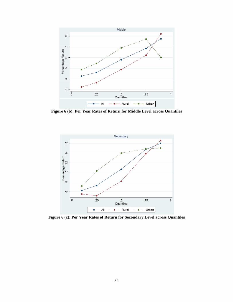
Using the estimates of Table 8, per year return to education across different

quantiles are computed in Table 9. The results of Table 9 are graphed in Figures 5(a) to

5(e) to show the rates of return of different educational levels in each quantile, and in

Figures 6(a) to 6(e) to show the rates of return of each educational level across different

quantiles. The following points are noticeable. First, rates of return to education are low

for lower levels of education and high for higher levels of education. In the 75th and 90th

quantiles, rates of return are highest for higher secondary level. The finding of low

returns in the 90th quantile is also evidenced by study of Blom et al. (2001). Second, these

findings are consistent in both rural and urban sectors, except for higher secondary level

in the rural sector where per year return to higher secondary level are low in 10th, 25th and

50th quantiles. Third, rates of return within educational levels differ across the wage

distribution. For primary, middle, secondary and higher secondary levels returns increase

across the quantiles (Figures 6(a)-6(d)). However, this pattern is not the same in the rural

and urban sectors. For graduation level, rates of return across quantiles are of an inverted

‘U shape’ (Figure-6e). This shows that the highest paid graduate workers possess lower

returns than the lower paid graduate workers. Blom et al. (2001) also find returns for

wealthier quantiles (75th and 90th) were lower than the less wealthy quantiles for tertiary

education in Brazil.

Tansel and Bircan (2010) find wage dispersion (difference between spread of 90th

and 10th quantiles, and spread of 75th and 25th quantiles) takes place mainly at the tails of

the wage distribution. We also find the same results in the Indian context. Table 10 shows

difference between the two spreads (.75-.25 spread, and .90-.10 spread). The spread of

90th and 10th quantiles is larger than the spread of 75th and 25th quantiles for all levels of

education. The results are consistent in both the sectors.

37 In our case, 90th quantile is the same as the 9th decile.

23

Finally, we show comparison of OLS and quantile regressions estimates for each

level of education graphically in Figures 7(a) to 7(e). The figures confirm both the mean

and median regressions are quite different. The quantile regression estimates of each

educational level lie outside the confidence intervals of the OLS regression. Quantile

regression methods capture a large disparity along the wage distribution and in this

manner these are quite helpful over OLS regression which assumes identical returns to

education in the same education group.

Our results are based on a specific cross-section dataset, which does not allow us

to find changes in the returns over a period of time. Therefore, we cannot say about

change in patterns of the returns. However, based on the past literature (Duraisamy, 2002;

Madheswaran & Attewll, 2007) it can be said that returns to higher education are

increasing. There are some possible reasons which could be attributed to higher returns

for higher education like introduction of new technologies which promotes the demand

for skilled labour especially those with higher education.

6. Conclusions

This paper estimates the private returns to education across different educational levels in

India. After correcting for the possibility of sample selection bias, the private returns to

education increase with the level of education. The findings in the paper thus do not

support the hypothesis of diminishing returns to education. The results for the earnings

function show that there is a substantial earnings difference between males and females.

Hourly wages of females are significantly lower than those of males by 38%. Across the

social groups, wages for STs and OBCs are significantly lower than those of ‘Others’ in

both rural and urban areas. Family background, as measured by household head’s

education is an important explanatory variable in explaining the wage equation. This

indicates it is important to identify individuals from poor family background and to

support their education. We find omitting the family background characteristics may bias

the returns upwards.

Using quantile regression, we examine the returns at different points of the wage

distribution. The returns to education differ along the wage distribution: the returns are

higher at the upper end of the wage distribution (higher decile/ quantile). The returns to

24

education within educational level also differ considerably. The rates of return increase

for primary, middle, secondary and higher secondary levels across the wage distribution.

For graduate workers per year returns are higher in the bottom quantiles. This shows that

education is not rewarded in a uniform manner in the labour market.

The increasing pattern of returns by level of education could be due to quality of

schooling. One can expect that quality of schooling may be ameliorating as an individual

ascends upwards in the educational hierarchy. Another reason which could explain this

phenomenon is ability of the people. If people with higher ability attain more schooling

then higher rates of return will be as a result of higher ability. However, we are not able

to account for both these factors in our analysis. The increasing pattern of private rates of

return suggests that for an individual, as a private decision, there is an incentive to invest

at higher secondary and graduate levels.

25

References

Agnarsson, Sveinn and Paul S. Carlin. 2002. "Family Background and the Estimated Return to Schooling: Swedish Evidence." The Journal of Human Resources, 37:3, pp. 680-92. Arrazola, María and José de Hevia. 2008. "Three Measures of Returns to Education: An Illustration for the Case of Spain." Economics of Education Review, 27:3, pp. 266–75. Azam, Mehtabul. 2009. "Changes in Wage Structure in Urban India 1983-2004: A Quantile Regression Decomposition." IZA Discussion Papaer No. 3963. Institute for the Study of Labor: Bonn, Germany. Becker, Gary S. 1993. Human Capital: A Theoretical and Empirical Analysis with Special Reference to Education. Chicago: University of Chicago Press [1st ed., 1964]. Belfield, Clive R. 2000. Economic Principles for Education: Theory and Evidence. Cheltenham, UK: Edward Elgar. Blom, Andreas, Lauritz Holm-Nielsen, and Dorte Verner. 2001. "Education, Earnings, and Inequality in Brazil, 1982-1998: Implications for Education Policy." Peabody Journal of Education, 76:3/4, pp. 180-221. Buchinsky, Moshe. 1998. "Recent Advances in Quantile Regression Models: A Practical Guideline for Empirical Research." The Journal of Human Resources, 33:1, pp. 88-126. Card, David. 1999. "The Causal Effect of Education on Earnings," in Handbook of Labour Economics. Orley Ashenfelter and David Card eds. Amsterdam: North-Holland. Chamarbagwala, Rubiana. 2010. "Economic Liberalization and Urban–Rural Inequality in India: A Quantile Regression Analysis." Empirical Economics, 39:2, pp. 371–94. Checchi, Daniele. 2006. The Economics of Education: Human Capital, Family Background and Inequality. Cambridge: Cambridge University Press. Desai, Sonalde, Amaresh Dubey, B.L. Joshi, Mitali Sen, Abusaleh Shariff, and Reeve Vanneman (undated). "India Human Development Survey: Design and Data Quality." India Human Development Survey Technical Paper No. 1. NCAER and University of Maryland. Duraisamy, P. 2002. "Changes in Returns to Education in India, 1983–94: By Gender, Age-Cohort and Location." Economics of Education Review, 21:6, pp. 609-22. Dutta, Puja Vasudeva. 2006. "Returns to Education: New Evidence for India,1983–1999." Education Economics, 14:4, pp. 431-51.

26

Falaris, Evangelos M. 2008. "A Quantile Regression Analysis of Wages in Panama." Review of Development Economics, 12:3, pp. 498–514. Griliches, Zvi. 1977. "Estimating the Returns to Schooling: Some Econometric Problems." Econometrica, 45:1, pp. 1-22. Halvorsen, Robert and Raymond Palmquist. 1980. "The Interpretation of Dummy Variables in Semilogarithmic Equations." The American Economic Review, 70:3, pp. 474-75. Harmon, Colm, Hessel Oosterbeek, and Ian Walker. 2003. "The Returns to Education: Microeconomics." Journal of Economic Surveys, 17:2, pp. 115-55. Hartog, Joop, Pedro T. Pereira, and José A. C. Vieira. 2001. "Changing Returns to Education in Portugal During the 1980s and Early 1990s: OLS and Quantile Regression Estimators." Applied Economics, 33:8, pp. 1021-37. Haveman, Robert, Barbara Wolfe, and James Spaulding. 1991. "Childhood Events and Circumstances Influencing High School Completion." Demography, 28:1, pp. 133-57. Heckman, James J. 1979. "Sample Selection Bias as a Specification Error." Econometrica, 47:1, pp. 153-61. Iversen, Vegard and Richard Palmer-Jones. 2008. "Literacy Sharing, Assortative Mating, or What? Labour Market Advantages and Proximate Illiteracy Revisited." Journal of Development Studies, 44:6, pp. 797–838. Kingdon, Geeta Gandhi. 1997. "Labour Force Participation, Returns to Education, and Sex Discrimination in India." The Indian Journal of Labour Economics, 40:3, pp. 507–26. Kingdon, Geeta Gandhi. 1998. "Does the Labour Market Explain Lower Female Schooling in India?" Journal of Development Studies, 35:1, pp. 39-65. Kingdon, Geeta Gandhi and Nicolas Theopold. 2006. "Do Returns to Education Matter to Schooling Participation? Evidence from India." Global Poverty Research Group Working Paper No. 52. Global Poverty Research Group. Koenker, R. & Bassett, G. (1978) Regression quantiles. Econometrica, 46(1), 33-50. Krishnan, Pramila. 1996. "Family Background, Education and Employment in Urban Ethiopia." Oxford Bulletin of Economics and Statistics, 58:1, pp. 167-83. Krueger, Alan B. and Mikael Lindahl. 2000. "Education for Growth: Why and for Whom?" NBER Working Paper No. 7591. NBER: Cambridge, MA.

27

Lam, David and Robert F. Schoeni. 1993. "Effects of Family Background on Earnings and Returns to Schooling: Evidence from Brazil." The Journal of Political Economy, 101:4, pp. 710-40. Machado, José A.F. and José Mata. 2001. "Earning Functions in Portugal 1982-1994: Evidence from Quantile Regressions." Empirical Economics, 26:1, pp. 115-34. Madheswaran, S and Paul Attewell. 2007. "Caste Discrimination in the Indian Urban Labour Market: Evidence from the National Sample Survey." Economic and Political Weekly, 42:41, pp. 4146-53. Martins, Pedro S. and Pedro T. Pereira. 2004. "Does Education Reduce Wage Inequality? Quantile Regressions Evidence from 16 Countries." Labour Economics, 11:3, pp. 355-71. Mincer, Jacob. 1974. Schooling, Experience and Earnings. New York: National Bureau of Economic Research. Moenjak, Thammarak and Christopher Worswick. 2003. "Vocational Education in Thailand: A Study of Choice and Returns." Economics of Education Review, 22, pp. 99-107. Moll, Peter G. 1996. "The Collapse of Primary Schooling Returns in South Africa 1960–90." Oxford Bulletin of Economics and Statistics, 58:1, pp. 185–209. Mwabu, Germano and T. Paul Schultz. 1996. "Education Returns Across Quantiles of the Wage Function: Alternative Explanations for Returns to Education by Race in South Africa." The American Economic Review, Papers and Proceedings, 86:2, pp. 335-39. Mwabu, Germano and T. Paul Schultz. 2000. "Wage Premiums for Education and Location of South African Workers, by Gender and Race." Economic Development and Cultural Change, 48:2, pp. 307-34. Oaxaca, Ronald. 1973. "Sex Discrimination in Wages," in Discrimination in Labor Markets. Orley Ashenfelter and Albert Rees eds. Princeton, New Jersey: Princeton University Press. Psacharopoulos, George. 1981. "Returns to Education: An Updated International Comparison." Comparative Education, 17:3, pp. 321-41. Psacharopoulos, George. 1985. "Returns to Education: A Further International Update and Implications." The Journal of Human Resources, 20:4, pp. 583-604. Psacharopoulos, George. 1994. "Returns to Investment in Education: A Global Update." World Development, 22:9, pp. 1325-43.

28

Psacharopoulos, George and Harry Anthony Patrions. 2004. "Returns to Investment in Education: A Further Update." Education Economics, 12:2, pp. 111-34. Schultz, T. Paul. 1988. "Education Investments and Returns," in Handbook of Development Economics. Hollis Chenery and T.N. Srinivasan eds. Amsterdam: North-Holland. Schultz, T. Paul. 2004. "Evidence of Returns to Schooling in Africa from Household Surveys: Monitoring and Restructuring the Market for Education." Journal of African Economies, 13 (Supplement 2, African Economic Research Consortium), pp. ii95-ii148. Siphambe, Happy Kufigwa. 2000. "Rates of Return to Education in Botswana." Economics of Education Review, 19, pp. 291-300. Swaminathan, Padmini. 2005. "Making Sense of Vocational Education Policies: A Comparative Assessment." The Indian Journal of Labour Economics, 48:3, pp. 537-51. Tansel, Aysit and Fatma Bircan. 2010. "Wage Inequality and Returns to Education in Turkey:A Quantile Regression Analysis." IZA Discussion Papaer No. 5417. Institute for the Study of Labor: Bonn, Germany. Tilak, Jandhyala B.G. 1987. The Economics of Inequality in Education. New Delhi: Sage Publications. Wooldridge, Jeffrey M. 2002. Econometric Analysis of Cross Section and Panel Data. London: The MIT Press.

29

Figures

Figure 1: Wage distribution for Male and Female in Rural Sector

Source: Author’s computation based on IHDS (2005) data.

Figure 2: Wage distribution for Male and Female in Urban Sector

Source: Author’s computation based on IHDS (2005) data.

30

Figure 3: Decile Rates of Return to Education

Figure 4: Comparison of OLS and Quantile Regression Estimates

Note: Dashed (horizontal) line shows OLS estimate and continuous line shows quantile regression estimates. Shaded region around both the lines shows confidence interval (95%).

31

Figure 5 (a): Per Year Rates of Return in the 10th Wage Quantile

Figure 5 (b): Per Year Rates of Return in the 25th Wage Quantile

32

Figure 5 (c): Per Year Rates of Return in the Median Wage Quantile

Figure 5 (d): Per Year Rates of Return in the 75th Wage Quantile

33

Figure 5 (e): Per Year Rates of Return in the 90th Wage Quantile

Figure 6 (a): Per Year Rates of Return for Primary Level across Quantiles

34

Figure 6 (b): Per Year Rates of Return for Middle Level across Quantiles

Figure 6 (c): Per Year Rates of Return for Secondary Level across Quantiles

35

Figure 6 (d): Per Year Rates of Return for Higher Secondary Level across Quantiles

Figure 6 (e): Per Year Rates of Return for Graduation Level across Quantiles

36

Figure 7 (a)

Figure 7 (b)

Figure 7 (c)

37

Figure 7 (d)

Figure 7 (e)

Figures 7 (a) -7 (e): Comparison of OLS and Quantile Regression Estimates by Educational

Level

Note: In each figure, the dashed (horizontal) line and the continuous line show the OLS estimate and quantile regression estimates, respectively. The two dotted lines and the shaded region around the continuous line depict 95% confidence intervals for the two estimates.

38

Tables

Table 1: Mean and Standard Deviation of Variables used in OLS Estimation

Variables All Rural Urban Log Hourly Wage 2.148 1.909 2.653

(0.818) (0.679) (0.854) Hourly Wage 12.675 8.990 20.458

(14.615) (9.799) (19.305) Educational Level Dummy Illiterate & Below Primary 0.391 0.478 0.207 Primary 0.143 0.153 0.121 Middle 0.150 0.145 0.158 Secondary 0.164 0.139 0.216 Higher Secondary 0.065 0.047 0.102 Graduate 0.087 0.037 0.194 Age 35.944 35.493 36.896

(11.886) 12.086) (11.393) Experience 25.552 (26.295 23.980

(13.376) (13.691) (12.541) Experience squared 831.794 878.894 732.305

(771.554) (803.452) (688.929) Sex (Dummy, Ref. -Male) 0.273 0.313 0.189 Sector (Dummy, Ref. -Rural) 0.321 - - Marital Status (Dummy, Ref.-Unmarried) 0.827 0.834 0.812 Social Group Dummy Others 0.244 0.184 0.372 OBC 0.381 0.378 0.389 SC 0.258 0.287 0.196 ST 0.116 0.151 0.043 Household Head Education Dummy Illiterate & Below Primary 0.589 0.672 0.415 Primary 0.173 0.167 0.184 Middle 0.097 0.080 0.135 Secondary and Higher Secondary 0.109 0.071 0.188 Graduate 0.032 0.010 0.078 Observations 46965 31875 15090

Note: The sample consists of individuals aged 15-65 in IHDS (2005) data. Standard deviation in parentheses, and is not reported for dummy variables. Refer Appendix I for the description of variables.

39

Table 2: Mean and Standard Deviation of Variables used in Heckman Estimation

Variables All Rural Urban Log Hourly Wage 2.148 1.909 2.653

(0.818) (0.679) (0.854) Hourly Wage 12.675 8.990 20.458

(14.615) (9.799) (19.305) Work Participation (Dummy) 0.467 0.542 0.362 Educational Level Dummy Illiterate & Below Primary 0.326 0.416 0.199 Primary 0.127 0.141 0.108 Middle 0.158 0.157 0.161 Secondary 0.203 0.175 0.243 Higher Secondary 0.095 0.069 0.132 Graduate 0.091 0.043 0.158 Age 33.494 33.354 33.691

(13.900) (14.052) (13.681) Experience 22.343 23.454 20.784

(15.937) (16.244) (15.362) Experience squared 753.216 813.956 667.966

(880.441) (924.686) (806.630) Sex (Dummy, Ref. -Male) 0.504 0.484 0.532 Sector (Dummy, Ref. -Rural) 0.416 - - Marital Status (Dummy, Ref.-Unmarried) 0.702 0.714 0.685 Social Group Dummy Others 0.314 0.240 0.419 OBC 0.384 0.390 0.376 SC 0.218 0.252 0.170 ST 0.084 0.118 0.035 Household Head Education Dummy Illiterate & Below Primary 0.434 0.550 0.271 Primary 0.169 0.180 0.154 Middle 0.128 0.109 0.154 Secondary and Higher Secondary 0.198 0.135 0.286 Graduate 0.071 0.026 0.135 Household Size 5.958 6.214 5.597

(2.927) (3.127) (2.577) Number of Children 1.668 1.874 1.379

(1.677) (1.787) (1.463) Non Labour Income (Dummy) 0.047 0.023 0.082 Observations 99900 58336 41564

Note: The sample consists of individuals aged 15-65 in IHDS (2005) data. Standard deviation in parentheses, and is not reported for dummy variables. Refer Appendix I for the description of variables.

40

Table 3: Mean Hourly Wages (in Rupees) by Educational Level and Gender

Educational Level Person Male FemaleIlliterate & Below Primary 6.84 8.25 5.16Primary 9.24 10.10 6.03Middle 10.96 11.68 7.16Secondary 15.47 16.00 11.04Higher Secondary 20.74 20.80 20.29Graduate 36.06 36.63 33.28All 12.68 14.50 7.82Note: The sample consists of individuals aged 15-65 in IHDS (2005) data. Refer Appendix I for the description of variables.

41

Table 4: Estimates of the Wage Equation

Variables Without Family Control

Family Control

State Control

Cohort Control

Selectivity Corrected

Human Capital Variables: Education 0.085*** 0.077*** 0.068*** 0.085*** 0.077***

(0.001) (0.001) (0.001) (0.001) (0.001)Experience 0.045*** 0.045*** 0.039*** 0.045*** 0.048***

(0.001) (0.001) (0.001) (0.001) (0.002)Experience squared -0.001*** -0.001*** -0.000*** -0.001*** -0.001***

(0.000) (0.000) (0.000) (0.000) (0.000) Demographic Variables:         (Ref: Male) Female -0.337*** -0.380*** -0.327*** -0.377*** -0.419***

(0.006) (0.007) (0.006) (0.007) (0.016) (Ref: Unmarried) Married -0.040*** -0.039*** -0.002 -0.029** -0.026*

(0.010) (0.009) (0.009) (0.010) (0.011) (Ref: Others) OBC -0.181*** -0.160*** -0.084*** -0.159*** -0.156***

(0.007) (0.007) (0.007) (0.007) (0.007) SC -0.114*** -0.090*** -0.062*** -0.089*** -0.085***

(0.008) (0.008) (0.008) (0.008) (0.009) ST -0.185*** -0.168*** -0.117*** -0.169*** -0.155***

(0.010) (0.010) (0.010) (0.010) (0.011) (Ref: Rural) Urban 0.384*** 0.359*** 0.353*** 0.358*** 0.352*** (0.006) (0.006) (0.006) (0.006) (0.007) Family Background Variable: (Ref: Head-Illiterate) Head –Primary 0.016* 0.003 0.015* 0.010

(0.008) (0.007) (0.008) (0.008)Head -Middle 0.042*** 0.028** 0.042*** 0.033**

(0.010) (0.009) (0.010) (0.010)Head -Secondary 0.137*** 0.118*** 0.138*** 0.122***

(0.010) (0.009) (0.010) (0.012)Head -Graduate 0.493*** 0.468*** 0.498*** 0.475***    (0.017) (0.016) (0.017) (0.018)Cohort Dummy (Ref: Age 15-29) Age 30-44 -0.123***

(0.011) Age 45-65 -0.075***

42

Variables Without Family Control

Family Control

State Control

Cohort Control

Selectivity Corrected

            (0.019) Intercept 1.445*** 1.499*** 1.824*** 1.415*** 1.474***

(0.017) (0.017) (0.026) (0.020) (0.019) Mills Lambda 0.050*

(0.020) R-squared 0.472 0.482 0.540 0.484 - Wald Chi2             42639 Total Observations 46965 46965 46965 46965 99900 Note: Dependent variable is log hourly wage. *, **, *** indicate significance levels at 10, 5 and 1% level of significance, respectively. Standard errors are in parentheses. In column 4 (state control), the coefficients of the state dummies are not reported. In column 6, only estimates of the wage equation are reported. Exclusion restrictions used in the probit equation (not reported) are household size, number of children in a household and non-labour income. Chi2 statistics are significant at p-value less than 0.00. Refer Appendix I for the description of variables.

43

Table 5: Selectivity Corrected (Heckman) Estimates of the Wage Equation using Educational Levels

Variables

All Rural Urban WE PE WE PE WE PE

Human Capital Variables: (Ref: Illiterate) Primary 0.164*** -0.068*** 0.139*** -0.063*** 0.198*** -0.034***

(0.009) (0.006) (0.010) (0.008) (0.020) (0.010) Middle 0.349*** -0.070*** 0.313*** -0.054*** 0.384*** -0.045***

(0.009) (0.006) (0.011) (0.009) (0.019) (0.009) Secondary 0.576*** -0.076*** 0.519*** -0.065*** 0.639*** -0.045***

(0.010) (0.007) (0.012) (0.009) (0.019) (0.009) Higher Secondary 0.820*** -0.038*** 0.711*** -0.054*** 0.932*** 0.004

(0.013) (0.009) (0.017) (0.013) (0.023) (0.012) Graduate 1.296*** 0.150*** 1.204*** 0.070*** 1.386*** 0.189***

(0.013) (0.009) (0.019) (0.014) (0.022) (0.013) Experience 0.049*** 0.043*** 0.047*** 0.043*** 0.058*** 0.039***

(0.001) (0.001) (0.002) (0.001) (0.003) (0.001) Experience squared -0.001*** -0.001*** -0.001*** -0.001*** -0.001*** -0.001***

(0.000) (0.000) (0.000) (0.000) (0.000) (0.000) Demographic Variables: (Ref: Male) Female -0.478*** -0.571*** -0.522*** -0.536*** -0.500*** -0.585***

(0.016) (0.004) (0.016) (0.006) (0.047) (0.006) (Ref: Unmarried) Married -0.021** 0.178*** -0.036*** 0.206*** 0.060*** 0.124***

(0.011) (0.006) (0.013) (0.008) (0.020) (0.008) (Ref: Others) OBC -0.141*** 0.083*** -0.139*** 0.106*** -0.136*** 0.050***

(0.007) (0.005) (0.009) (0.006) (0.013) (0.006) SC -0.074*** 0.123*** -0.083*** 0.147*** -0.037** 0.079***

(0.008) (0.006) (0.010) (0.007) (0.016) (0.008) ST -0.156*** 0.223*** -0.191*** 0.230*** 0.103*** 0.152***

(0.011) (0.007) (0.013) (0.007) (0.028) (0.017) (Ref: Rural) Urban 0.343*** -0.140*** - - - -

(0.007) (0.004) Family Background Variable: (Ref: Head- Illiterate) Head -Primary 0.033*** -0.074*** 0.026*** -0.073*** 0.036** -0.069***

(0.008) (0.005) (0.009) (0.007) (0.015) (0.008) Head -Middle 0.045*** -0.134*** 0.026** -0.133*** 0.062*** -0.121***

44

Variables

All Rural Urban WE PE WE PE WE PE

(0.010) (0.006) (0.013) (0.008) (0.019) (0.007) Head -Secondary 0.099*** -0.213*** 0.047*** -0.226*** 0.133*** -0.184***

(0.011) (0.005) (0.015) (0.008) (0.020) (0.007) Head -Graduate 0.338*** -0.253*** 0.306*** -0.290*** 0.343*** -0.207***

(0.019) (0.007) (0.034) (0.015) (0.028) (0.007) Exclusion Variables: Household Size -0.038*** -0.041*** -0.028***

(0.001) (0.001) (0.002) No. of Children 0.034*** 0.037*** 0.025***

(0.002) (0.002) (0.003) Non Labour Income -0.108*** -0.126*** -0.091***

(0.009) (0.018) (0.009) Intercept 1.617*** - 1.738*** - 1.691*** -

(0.019) (0.025) (0.033) Mills Lambda 0.075*** 0.152*** 0.088**

(0.020) (0.024) (0.043) Wald Chi2 43661 14596 10419 Total Observations 99900 58336 41564

Note: Dependent variable is log hourly wage. WE and PE are Wage and Participation Equations, respectively and for PE marginal effect is reported. *, **, *** indicate significance levels at 10, 5 and 1% level of significance, respectively. Standard errors are in parentheses. Chi2 statistics are significant at p-value less than 0.00. Refer Appendix I for the description of variables.

45

Table 6: Private Rates of Return to Education (%)

Educational Level All Rural UrbanPrimary 5.47 4.64 6.59 Middle 6.15 5.80 6.20 Secondary 11.38 10.29 12.73 Higher Secondary 12.21 9.60 14.67 Graduate 15.87 16.43 15.12

Note: The results are computed using Table 5. For example, private rate of return for middle level can be computed as: rmiddle = (βmiddle- βprimary)/∆nmiddle = (0.349-0.164)/3= 0.061 or 6.15%.

Table 7: Decile Rates of Return to Education

Decile All Rural Urban 0.1 0.038*** 0.026*** 0.064***

(0.001) (0.002) (0.003) 0.2 0.044*** 0.030*** 0.075***

(0.001) (0.001) (0.002) 0.3 0.051*** 0.032*** 0.084***

(0.001) (0.001) (0.002) 0.4 0.061*** 0.037*** 0.093***

(0.001) (0.001) (0.002) 0.5 0.071*** 0.049*** 0.098***

(0.001) (0.001) (0.001) 0.6 0.080*** 0.062*** 0.101***

(0.001) (0.001) (0.002) 0.7 0.090*** 0.077*** 0.101***

(0.001) (0.002) (0.002) 0.8 0.097*** 0.093*** 0.100***

(0.001) (0.002) (0.002) 0.9 0.104*** 0.105*** 0.098***

(0.001) (0.002) (0.002) Note: Dependent variable is log hourly wage. *, **, *** indicate significance

levels at 10, 5 and 1% level of significance, respectively. Bootstrap standard errors (with 600 repetitions) are in parentheses. Only regression coefficient of education is reported for each decile. F-test is carried out to check equality of coefficients across deciles. The test statistics are F (8, 46951) = 235.11 for All, F (8, 31862) = 235.53 for Rural, and F (8, 15077) = 27.80 for Urban with p-value less than 0.00 in all cases.

46

Table 8: Estimates of Quantile Regression using Educational Levels

Educational Level Quantile Group 0.10 0.25 0.50 0.75 0.90

All Population Primary 0.045*** 0.062*** 0.121*** 0.246*** 0.337***

(0.011) (0.009) (0.009) (0.013) (0.018) Middle 0.173*** 0.200*** 0.295*** 0.452*** 0.569***

(0.015) (0.009) (0.010) (0.013) (0.017) Secondary 0.297*** 0.345*** 0.508*** 0.748*** 0.889***

(0.016) (0.012) (0.012) (0.015) (0.019) Higher Secondary 0.342*** 0.493*** 0.769*** 1.097*** 1.226***

(0.025) (0.020) (0.022) (0.021) (0.026) Graduate 0.790*** 1.053*** 1.315*** 1.537*** 1.604***

(0.028) (0.023) (0.016) (0.019) (0.020) Rural Primary 0.046** 0.056*** 0.086*** 0.215*** 0.313***

(0.015) (0.011) (0.010) (0.014) (0.020) Middle 0.143*** 0.166*** 0.232*** 0.401*** 0.559***

(0.017) (0.012) (0.010) (0.017) (0.023) Secondary 0.253*** 0.269*** 0.395*** 0.678*** 0.891***

(0.020) (0.012) (0.014) (0.020) (0.024) Higher Secondary 0.223*** 0.329*** 0.537*** 1.054*** 1.291***

(0.032) (0.020) (0.030) (0.034) (0.038) Graduate 0.535*** 0.710*** 1.196*** 1.629*** 1.716***

(0.036) (0.047) (0.039) (0.031) (0.036) Urban Primary 0.071** 0.121*** 0.217*** 0.273*** 0.295***

(0.025) (0.021) (0.023) (0.022) (0.035) Middle 0.217*** 0.284*** 0.424*** 0.505*** 0.476***

(0.026) (0.022) (0.023) (0.021) (0.031) Secondary 0.360*** 0.489*** 0.704*** 0.802*** 0.776***

(0.026) (0.024) (0.024) (0.023) (0.029) Higher Secondary 0.549*** 0.753*** 1.037*** 1.100*** 1.049***

(0.038) (0.032) (0.030) (0.026) (0.032) Graduate 1.035*** 1.291*** 1.481*** 1.496*** 1.448***

(0.041) (0.034) (0.028) (0.026) (0.032) Note: Dependent variable is log hourly wage. *, **, *** indicate significance levels at 10, 5 and

1% level of significance, respectively. Bootstrap standard errors (with 600 repetitions) are in parentheses. Only regression coefficient of education is reported for each quantile. F-test is carried out to check equality of coefficients across deciles. See, Appendix II for the statistic.

47

Table 9: Per Year Quantile Rates of Return by Educational Level (%)

Educational Level Quantile Group 0.10 0.25 0.50 0.75 0.90

All Population Primary 1.50 2.06 4.03 8.22 11.22 Middle 4.26 4.60 5.80 6.86 7.76 Secondary 6.23 7.27 10.64 14.76 15.99 Higher Secondary 2.25 7.38 13.07 17.48 16.85 Graduate 14.90 18.66 18.19 14.65 12.59 Rural Primary 1.52 1.87 2.86 7.17 10.42 Middle 3.24 3.65 4.88 6.21 8.22 Secondary 5.50 5.15 8.16 13.86 16.58 Higher Secondary -1.49 3.00 7.08 18.79 20.01 Graduate 10.41 12.71 21.96 19.16 14.18 Urban Primary 2.35 4.03 7.24 9.11 9.84 Middle 4.88 5.44 6.90 7.73 6.01 Secondary 7.16 10.25 13.99 14.87 15.03 Higher Secondary 9.45 13.19 16.68 14.86 13.65 Graduate 16.20 17.92 14.80 13.21 13.31

Note: The results are computed using Table 8. See, also note of Table 6

Table 10: Wage Dispersion across the Wage Distribution

Educational All Rural Urban Level Q.75-Q.25 Q.90-Q.10 Q.75-Q.25 Q.90-Q.10 Q.75-Q.25 Q.90-Q.10Primary 0.18 0.29 0.16 0.27 0.15 0.22 Middle 0.25 0.40 0.24 0.42 0.22 0.26 Secondary 0.40 0.59 0.41 0.64 0.31 0.42 Higher Secondary 0.60 0.88 0.73 1.07 0.35 0.50 Graduate 0.48 0.81 0.92 1.18 0.21 0.41 Note: Q75-Q25 and Q90-Q10 denote spread of 75th and 25th quantiles, and spread of 90th and 10th quantiles, respectively. Source: Table 8.

48

Appendix I: Description of Variables used in the Estimation

Variable Description Base category Explained (Dependent)Variables Log Hourly Wage Natural Logarithm of hourly wages in

rupees. Explained variable in the wage equation. Quantile Regression Wage Decile: 0.1, 0.2, 0.3, 0.4, 0.5, 0.6, 0.7, 0.8, and 0.9 deciles when education is used as a continuous variable. Wage Quantile: 0.1, 0.25, 0.5, 0.75, and 0.9 quantiles when education is used as a categorical variable.

None

Work Participation If an individual works more than or equal to 240 hours in a year, he/she is considered as a part of the workforce. a Explained variable in probit equation.

If an individual works less than 240 hours in a year.

Explanatory (Independent) Variables Human Capital Variables Educational Level (5 dummies: Primary, Middle, Secondary, Higher Secondary, and Graduate)

An individual belongs to one of the following educational level: Illiterate (includes literate with below primary also), Primary, Middle, Secondary, Higher Secondary, and Graduate. It is assumed that an individual spends 0, 5, 3, 2, 2 and 3 additional years, respectively in these educational levels.

Illiterate (and literate with below Primary)

Experience Potential experience (proxy for the actual labour market experience) in years, defined as: Age-Years of schooling-5.b

None

Experience squared Square of Experience None Demographic Variables Gender (Female) Sex of individual: Male or Female Male Sector (Urban) Place of residence: Rural or Urban Rural Marital Status Marital Status of individual: Never married

(unmarried), and Married (also includes Divorced, Widowed and others)

Unmarried

Social Group (3 dummies: SC, ST and OBC)

Each household belong to one of the following social groups: Scheduled Castes (SCs), Scheduled Tribes (STs), Other Backward Classes (OBCs) and Others.

Others

Age Cohort (2 dummies: Cohort 30-44, and Cohort 45-65)

Working population is classified into three age cohorts: Cohort 15-29 (if individual’s age lies 15-29 years), Cohort 30-44 if individual’s age lies 30-44 years), and Cohort 45-65 (if individual’s age lies 45-65 years).

Cohort 15-29

State dummies (32 dummies)

One dummy corresponding to each state/union territory.

State of Jammu and Kashmir

49

Family Background Variable Household Head’s Education (4 dummies: Head-Primary, Head-Middle, Head-Secondary, and Head- Graduate

Education of household head, which is grouped as Illiterate (and literate with below primary), Primary, Middle, Secondary and Higher Secondary, and Graduate.c

Head-Illiterate

Exclusion Restrictions Household Size Number of members in a household None No. of Children Number of children (aged 0-14) in a

household None

Non Labour Income Non labour income includes income from renting property and/or income from interest, dividends, or capital gains.

Household does not have non labour income.

Note: Description of variables is based on IHDS (2005) data. a The criterion for selection of 240 hours in a year is based on work participation measure used in the IHDS data. b It is assumed that an individual starts schooling at the age of five and starts working immediately after schooling. c In case, where household head him/herself is considered as an individual his/her father’s education is taken as household head’s education.

50

Appendix II: Tests of Equality of Coefficients of Education Dummy across Quantiles

Education (Dummy) All Rural Urban Primary F(4, 46947) = 66.69 F(4, 31858) = 50.04 F(4, 15073) = 13.12Middle F(4, 46947) = 119.77 F(4, 31858) = 76.06 F(4, 15073) = 25.02Secondary F(4, 46947) = 214.36 F(4, 31858) = 177.51 F(4, 15073) = 58.89Higher Secondary F(4, 46947) = 219.99 F(4, 31858) = 195.78 F(4, 15073) = 49.47Graduate F(4, 46947) = 180.87 F(4, 31858) = 189.43 F(4, 15073) = 34.81

Note: In all cases p-values are less than 0.00.