Final Report

RETROFIT CATHODIC PROTECTIONOF MARINE PIPELINES ASSOCIATED

WITH PETROLEUM PRODUCTION

submitted to

Minerals Management ServiceU.S. Department of the Interior

381 Elder RoadHerndon, Virginia 22070

by

William H. Hartt, Diane Lysogorski, Haijun Qian,Keith Bethune, and Patrick Pierson,

Center for Marine MaterialsDepartment of Ocean Engineering

Florida Atlantic University – Sea Tech Campus101 North Beach Road

Dania Beach, Florida 33004

August 7, 2001

TECHNICAL SUMMARY

Marine oil and gas transportation pipelines have been in service in the Gulf of Mexico for almost 50

years. These lines are invariably protected from external corrosion by a combination of coatings and

cathodic protection (cp); however, the design life of such protection systems upon older lines has now been

exceeded in many cases such that some have required, and others will soon require, cp retrofitting. In

response to this, the present project was initiated in 1997 for the purpose of establishing criteria and

protocols for design of marine pipeline retrofit cp systems. Five research tasks were identified and

addressed as:

I. Development of a New Approach to Cathodic Protection Design for New Marine Pipelines.

II. Development of An Inclusive, First Principles Based Attenuation Model for Marine Pipeline Cathodic Protection.

III. Verification of the Proposed Cathodic Protection Design Method and Attenuation Model.

IV. Definition and Examination of Critical Issues Related to Pipeline Cathodic Protection Retrofits.

V. Recommended Protocol for Retrofit Cathodic Protection Design of Marine Pipelines.

As background, a critical review and state-of-the-art summary for cp of petroleum production structures

was conducted. This focused first upon cp of platforms, since the technology for these is more mature, and

then proceeds to pipelines. Particular attention is given to the recent development of a unified, first-

principles based design equation and cp design protocol termed the Slope Parameter Method. Within the

above tasks, critical aspects of pipeline retrofit cp design have been identified; and it is demonstrated that

the decision path and governing features for cp retrofits of pipelines are distinct from those associated with

new construction. Specifically, Task IV identifies 1) determination of pipe cp current density demand, 2)

optimization of retrofit anode array spacing, and 3) anode array design as particularly critical. Methods

whereby Items 1 and 2 can be addressed are based upon the results from Tasks I and II, and Task III

provides verification for these. The cornerstone of these efforts is, first, modification of the Unified Design

Equation to pipelines and, second, development of a first-principles based potential attenuation and anode

current output equation for pipelines. Protocol options for accomplishment of Item 3 (anode array design),

on the other hand, are developed from the literature. Lastly, a flow chart that integrates these different cp

design components is presented and discussed under Task V.

ii

TABLE OF CONTENTS

1. EXECUTIVE SUMMARY ii

2. TABLE OF CONTENTS iii

3. NOMENCLATURE v

4. INTRODUCTION 1

General 1Corrosion Control for Marine Pipelines 1Aging Marine Pipeline Infrastructure 2Cathodic Protection Design Protocol for Offshore Structures 3

General 3Platforms 4Pipelines 8

Corrosion and CP Assessment Methods 9Existing Pipeline Cathodic Protection System Analysis Methods 10

5. PROJECT OBJECTIVES 13

6. TASK I: DEVELOPMENT OF A NEW APPROACH TO CATHODICPROTECTION DESIGN FOR NEW PIPELINES 13

Development of Equations 13Example Pipeline CP Design 16

7. TASK II: DEVELOPMENT OF AN INCLUSIVE, FIRST-PRINCIPLESBASED ATTENUATION MODEL FOR MARINE PIPELINECATHODIC PROTECTION 17

General 17The Governing Equation 17

8. TASK III: VERIFICATION OF THE PROPOSED CATHODIC PROTECTIONDESIGN METHOD AND ATTENUATION MODEL 20

Attenuation Equation 20Effect of Anode Spacing and Pipe Current Demand upon Potential

Attenuation and Anode Current Output 24Slope Parameter Method 27

Comparison with FDM Solutions 27Range of Applicability of the Slope Parameter Design Approach 28

9. TASK IV: DEFINITION AND EXAMINATION OF CRITICAL ISSUESRELATED TO PIPELINE CATHODIC PROTECTION RETROFITS 30

Detection of pipeline Anode Expiration 30Principle Design Parameters for Pipeline CP Retrofits 32Pipeline Current Density Demand 33Example Calculation of Pipe Current Density Demand 33Anode/Anode Array Design 37Maximized Anode/Anode Array Spacing 41

iii

10. TASK V: RECOMMENDED PROTOCOL FOR RETROFIT CATHODICPROTECTION DESIGN OF MARINE PIPELINES 50

11. BIBLIOGRAPHY 52

12. APPENDIX A: Derivation of the First-Principles Pipeline Attenuation Equation 54

13. APPENDIX B: Spacing Distance between Crossing Pipelines

iv

NOMENCLATURE

Aa: Anode surface area. Ac: Structure (cathode) surface area. Ac(1): Pipe surface area protected by a single anode. C: Anode current capacity. d: Distance from a offset anode to a position on a pipeline. D: Diameter of a circle about with an array of equally spaced anodes are placed. Ea: Magnitude of cathodic polarization at z = 0. Eb: Magnitude of cathodic polarization at z = L. Ec(z): Magnitude of cathodic polarization at z. fc: Coating breakdown factor (fraction of the external pipe surface that is exposed at coating defects

and bare areas). io: Initial cathodic protection design current density. im: Mean cathodic protection design current density. if: Final cathodic protection design current density. ic: Structure (cathode) current density demand. ic(z): Cathodic current density at z along a pipeline. Ia: Current output of an individual anode. Im(z): Metallic path current in a pipeline at z. k: Polarization resistance of bare metal exposed at coating defects. l: Length of an individual stand-off anode. L: Half spacing between equally spaced anodes. Las: Anode spacing. M: Total anode mass. N: Number of galvanic anode. OF: Distance from an offset anode and a pipeline r: Anode radius or effective radius. ra: Equivalent radius of a spherical anode. Rp: Pipeline radius. R: Resistance. R(N): Resistance of an array of N anodes. Ra: Resistance of an individual anode. Rt: Total cathodic protection circuit resistance. Rm: Pipeline metallic path resistance per unit length. S: Distance between equally spaced anodes in a linear array. S: Slope parameter. Sa: Surface area of a cylindrical anode. T: Cathodic protection system design life. u: Anode utilization factor. Um(z): Potential on the pipe side of the double layer. Ue(z): Electrolyte potential just outside the double layer. v: Volume fraction of the anode that is galvanic metal as opposed to core. w: Weight of an individual galvanic anode. z: Distance along a pipeline from an anode.

a’: Attenuation factor. a: Polarization resistance. fa: Closed circuit anode potential. fc: Closed circuit cathode potential. fcorr: Corrosion potential. fc(z): Polarized pipe potential at z. fc(FF): Polarized pipe potential at large z. fc(Av): Average polarized pipe potential. g: Ratio of total pipe surface area to bare surface area.

v

r’: Anode density. re: Electrolyte resistivity. z: Coating resistance per unit length.

vi

INTRODUCTION

General

There are in excess of 30,000 miles (48,000 km) of crude oil and gas marine pipelines in U.S. and

state waters. While such pipelines are generally recognized as the safest, efficient, and cost effective means

of transportation for offshore oil and gas from fixed production facilities, still failures occur because of 1)

material and equipment problems, 2) operational errors, 3) corrosion, 4) storm/mud slides, and 5) third

party incidents (mechanical damage). These, in turn, can result in loss of life, pollution, loss of product

availability, repair expenses, business interruption, and litigation. Several publications (1-4) and a data

base (5) have documented and evaluated the occurrence and causes of offshore pipeline failures that have

taken place historically in the Gulf of Mexico and elsewhere. Each of these indicates that the major cause

has been corrosion, with MMS data attributing over 50 percent of the failures to this mode. Of these,

approximately 63 percent have occurred on pipelines as opposed to risers; and 69 percent resulted from

external, as opposed to internal, corrosion. At the same time, however, only 12 percent of the external

corrosion failures were on pipelines, with 88 percent being on risers. On the one hand, this indicates the

susceptibility that prevails in the vicinity of the water surface, where corrosion rate is generally greatest.

On the other, such failures are normally detected prior to substantial product discharge and are relatively

inexpensive to repair. However, such data probably understates the role of corrosion, since instances where

a pipeline has been weakened by corrosion but failed from an alternative cause (storm or third party

damage, for example) are invariably attributed to the latter and not the former. Additional concerns with

regard to pipeline corrosion failures are that, first, the average failure rate during the 1990’s was more than

double that of the 1980’s; second, the increased focus in the Gulf of Mexico upon deep water production

indicates that failures, where they occur, will be more difficult and expensive to address; and, third, the

cathodic protection system design life for many older pipelines has now been exceeded such that external

corrosion may be ongoing and cathodic protection retrofitting required. At the same time, no standardized

procedure presently exists for design of retrofit cathodic protection systems for marine pipelines. Increased

attention has, however, been directed in recent years toward this specific problem; that is, external

corrosion of marine oil and gas pipelines, as evidenced by the fact that a 1991 International Workshop on

Offshore Pipeline Safety (6) included only one paper that explicitly addressed corrosion and corrosion

control; but a more recent MMS International Workshop (7) focused specifically upon this topic.

Corrosion Control for Marine Pipelines

Structural and high strength steels have historically been the only economically viable material for

construction of marine petroleum transport pipelines. However, the inherent lack of corrosion resistance of

this material class in sea water and the consequences of pipeline failure require that corrosion control

systems be designed, installed, and maintained such that a high degree of reliability is realized. Reliability

considerations have become magnified in recent years with the transition from relatively shallow to

deepwater installations. While cathodic protection (cp) has historically been employed as the sole

corrosion control methodology for the submerged portion of petroleum production platforms, both mobile

and fixed, the one-dimensional nature of pipelines is such that the combined use of coatings with cp is

required. In the former case (platforms), anode resistance and structure current density demand are the

fundamental parameters that are important in cp design. For pipelines, however, coating quality and

metallic path (pipeline) resistance must also be taken into account, at least in the generalized case.

Cathodic protection systems, either for pipelines or for other engineering applications, can be of either the

impressed current (ic) or galvanic anode (ga) type. For marine pipelines, however, iccp systems are

invariably limited to 1) proximity of landfall where protection can be provided seaward by a shore-based

rectifier and anode array to a distance that is defined by the “throwing power” of the system and 2) pipeline

runs between two platforms where the distance is sufficiently short that the entire line can be protected by a

single rectifier and anode or anode template at one or both ends. In either case (shore or platform-based

iccp), the limiting distance to which corrosion protection can be affected is normally limited by the voltage

drop along the metallic pipeline that arises in conjunction with the current return to ground. An additional

factor that affects the distance to which corrosion protection is afforded is quality of the protective coating.

Thus, the higher the coating quality, the less the pipe current demand and, as a consequence, the less the

voltage drop for a pipeline of a given length. However, coating quality of marine pipelines is invariably

below that of buried onshore counterparts so that this distance of protection is considerably less in the

former case than the latter. Also, coating quality, as defined by capacity of the coating to isolate the

underlying steel, decreases with time; and, consequently, the distance to which protection is extended also

becomes reduced. In order to maximize the distance to which protection is achieved, the region of the

pipeline near the rectifier and anode array may be overprotected. Such overprotection can cause coating

damage in the form of blistering and disbondment, in which case the pipe current demand increases.

Because of these factors, corrosion control for the great majority of marine pipelines is provided by

galvanic anodes (gacp); and for structural, economic, and installation considerations these are invariably of

the bracelet type, as illustrated schematically in Figure 1. For these same reasons (structural and

installation considerations) the size and, hence, weight of bracelet anodes is limited such that the spacing

between anodes is, according to current practice, only about 750 feet (250 meters). Consequently, voltage

drop in the pipeline is insignificant; and cp system life is governed by anode mass considerations alone.

Aging Marine Pipeline Infrastructure

Marine pipelines have been in service in the Gulf of Mexico since the 1940’s. At the same time,

cathodic protection systems for these are typically designed for 25-30 years. Consequently, the design life

for the cp system of many older lines has been exceeded and for others is being approached. Also, earlier

2

Anode

Pipe

Figure 1: Schematic illustration of an offshore pipeline galvanic anode.

cp designs were typically less conservative than is the current practice; and anode quality was less. Thus, a

one-quarter mile (400 m) bracelet anode spacing was commonly specified several decades ago. However,

it is not uncommon for the electrical connection of an anode to the pipeline to become damaged or for the

anode to become otherwise compromised during pipeline installation, which results in an effective

doubling of the anode spacing. Deficient quality of anodes was invariably in the form of faulty chemistry,

as can still occur today, such that 1) the pipeline failed to polarize, as explained below, or 2) anode

consumption rate was high (low current capacity), or both. In either case (cp design life exceedance or lack

of anode performance), external corrosion protection on older marine pipelines either may have been or is

in the process of being lost. Consequently, pipeline cp retrofits have become increasingly common, both in

the Gulf of Mexico and elsewhere; and the frequency of retrofits in the future is likely to become greater.

Cathodic Protection Design Protocol for Offshore Structures

General

It is generally recognized that corrosion of steel in sea water is arrested by polarization to a potential

of –0.80 VAgCl or more negative, and so achieving and maintaining a minimum polarization based upon this

potential has been established as the goal of cathodic protection (8-10) irrespective of the type of structure

involved (pipeline, platform, ship, and so on). Figure 2 illustrates schematically a pipeline with identical,

equally spaced bracelet anodes and the resultant polarized potential profile. Thus, the pipeline is most

polarized immediate to the anodes; and potential attenuates with increasing distance therefrom. Four

factors determine the magnitude of this potential attenuation, as listed below:

1. Anode resistance. This resistance is encountered as current leaves the anode and enters the electrolyte. It is a consequence of the geometrical confinement in the vicinity of the anode. Accordingly, attenuation from this cause is greatest immediate to the anode and decreases with increasing distance. Anode resistance is higher the greater the electrolyte resistivity and the smaller the anode.

2. Coating resistance. The intrinsic resistivity of marine pipeline coatings is relatively high; however, coating defects and bare areas from handling, transportation, and installation are

3

Polarization = Ea Polarization = Eb

2L Anode

Pipeline

at z = L

z=0

at z = 0

UN

DE

RP

RO

TE

CT

ION

PO

TE

NT

IAL

+

-

POSITION ALONG PIPELINE

-0.80v (Ag-AgCl)

Polarization = E ATz DISTANCE z

ALONG PIPELINE

Figure 2: Schematic illustration of a cathodically polarized pipeline and the resultant potential profile.

invariably present. Consequently, the cp current enters the pipe at these locations where steel is directly exposed. Thus, the coating serves to reduce the exposed surface area of the pipeline compared to an uncoated situation, which, in turn, enhances the effectiveness, efficiency, and distance to which protection is achieved.

3. Polarization resistance. This resistance term reflects an inherent resistance associated with the cathodic electrochemical reaction whereby ionic current in the electrolyte is translated to electronic conduction in the pipeline.

4. Metallic resistance. Although resistivity of steel is orders of magnitude less that that of sea water, the confined pipeline cross section combined with the relatively long distance that current may have to travel in returning to electrical ground results in this term being influential, if not controlling, in some situations.

Portions of a pipeline for which potential is –0.80 VAgCl or more negative are protected, whereas locations

where potential is more positive are unprotected. Specific protocols that apply to cathodic protection

design of platforms and pipelines are discussed below.

Platforms

Cathodic protection design procedures have evolved historically according to:

1. Trial and error.

4

2. Ohm’s law employing a single, long-term current density (11).

3. Ohm’s law and rapid polarization employing three design current densities, an initial (io), mean,

(im), and final (if) (8,9).

4. The slope parameter method (12-15).

Accordingly, practices 2) and 3) are based upon the equation

fc -faI a = , (1Ra

where

Ia = individual anode current output,

fc = closed circuit cathode potential,

fa = closed circuit anode potential, and

Ra = resistance of an individual anode.

As noted above, anode resistance is normally the dominant component of the total circuit resistance for

space-frame structures such as platforms, and so it alone need be considered here. In most cases, this

parameter is calculated from standard, numerical relationships that are available in the literature (16-21)

based upon anode dimensions and electrolyte resistivity. Figure 3 graphically illustrates the principle

behind this equation and approach.

Considering that the net current for protection, Ic, is the product of the structure current density

demand (ic) and surface area (Ac), the number of anodes required for protection, N, is determined from the

relationship

i � A N = c c . (2

I a

By earlier practice (11), cp design was based upon a single, time average or mean current density that

polarized the structure to the potential required for protection (-0.80 VAgCl) within perhaps several months

to one year. It was subsequently recognized, however, that application of an initially high current density

(rapid polarization (21-26)) resulted in a lower mean current density and reduced anode mass to provide

protection for the design life. Accordingly, present protocols (8,9) are based upon three current densities,

an initial (io), mean (im), and final (if), where the first is relatively high and is realized upon initial

deployment, the second is the time-averaged value, and the last reflects what is required near the end of the

5

fcorr (Steel)

f-I Kinetics for

- POT

EN

TIA

L,

Vag

/AgC

l +

Oxygen Reduction

I a

f corr (Anode)

f c

f a

IaRa

CURRENT

Figure 3: Schematic illustration of a polarization diagram and of parameters relevant to galvanic anode cathodic protection system design.

design life to affect repolarization should this become necessary. The required number of anodes

corresponding to the respective values for io and if is determined by substituting each of these parameters

for ic in Equation 2. On the other hand, im is calculated from the mass balance relationship,

8,760 � i � A � T N = m c , (3

u � C � w

where

T = design life of the cp system (years),

u = utilization factor (see Table 2),

C = anode current capacity ( A � h/kg ), and

w = weight of an individual anode (kg).

Invariably, the number of anodes determined according to each of the three calculations is different with

the largest being specified. For uncoated structures this is usually io. Consequently, the system is over-

designed in terms of the other two current densities. This arises because the procedure is an algorithm

rather than being first principles based.

More recently, the slope parameter approach to galvanic cp system design (12-15) was developed

6

Table 2: typical anode utilization factors recommended for cp design (10).

Anode Type Utilization Factor, unitless

Long1 Slender Stand-Off Long1 Flush-Mounted Short2 Flush-Mounted Bracelet, Half-Shell Type Bracelet, Segmented Type

0.90 0.85 0.80 0.80 0.75

1. Anode length ‡ 4 x thickness. 2. Anode length < 4 x thickness.

based upon a modification of Equation 1 as,

fc = (Rt � Ac )� ic + fa , (4

where Rt is the total circuit resistance. This relationship projects a linear interdependence between fc and ic

provided Rt, Ac, and fa are constant. That this is normally the case has been confirmed by both laboratory

and field measurements (12-15). For space frame type structures with multiple galvanic anodes,

R Rt @ a ; (5

N

with the product Rt � Ac (Equation 4) being defined as the slope parameter, S, such that,

Ra � AcS = . (6N

Substitution of the latter expression into Equation 4 then yields,

i �T � S Ra � w = m , (7

C

which is referred to as the Unified Design Equation. Upon defining an appropriate value for S, all terms on

the right side are known from the design choices. An anode type is then either selected or designed based

upon the optimum combination of Ra and w. This may be accomplished in terms of anodes of standard

dimensions or, perhaps more effectively, by specifying an elongated anode or dualnodes (27). Thus, if

anode resistance is represented in terms of Dwight’s modified equation,

7

Ra = r e � Œ

Øln�

� 4l �� -1œ

ø , (8

2pl º Ł r ł ß

where

re = electrolyte resistivity,

l = anode length, and

r = equivalent anode radius,

then the left side of Equation 7 becomes

r � r ' � r 2 �v Ø 4L øRa � w = Œln -1œ , (9

2 º r ß

where

r’ = anode density and

v = volume fraction of the anode that is galvanic metal as opposed to core.

The required number of anodes can then be calculated from Equation 6.

Hartt et al. (13) projected that the slope parameter based design approach yields a 32 percent

reduction in anode mass in the case of typically sized structures compared to design according to present

recommended practice 9,10). This arises because Equation 7 is first principles based and incorporates both

im and io, the former explicitly and the latter implicitly via the slope parameter. As such, design can be

optimized in terms of both parameters instead of just one. An alternative view is that, of the two terms on

the left side of Equation 7, Ra determines io while w relates to im.

Pipelines

There are two fundamental differences between offshore platforms and pipelines: first, the three

dimensional nature of the former compared to one dimensional for the latter and, second, the fact that

pipelines are invariably coated while platforms are normally not. The same three design current densities,

io, im, and if, are employed; however, marine pipeline cp design (9,10) considers the current demand, Ic, as

I c = Ac � f c � ic , (10

where fc is the fraction of the external pipe surface that is exposed at coating defects and bare areas. Design

values for io and if are normally in the range 5.6-20 mA/ft2 (60-220 mA/m2) (bare surface area basis)

8

depending upon pipe depth, temperature, sea water versus mud exposure, and whether or not the

calculation is for the initial (Ic = Io) or final (Ic = If) condition. As for platforms, the design is accomplished

by substituting io and if for ic and calculating the corresponding Ic. The net anode mass, M, on the other

hand is determined from a modified form of Equation 3 as,

8,760 � I m �T M = , (11

u �C

where Im is the mean current to protect the pipeline. The required number of anodes is then determined

considering the values for Io, If, and M. As noted above, the limiting feature of the pipeline cp design

protocol is the maximum permissible anode bracelet size, as determined by structural and installation

considerations. Because bracelet anodes are relatively small, so also is their spacing along the pipeline.

This, in turn, results in metallic path resistance and voltage drop being negligible such that these need not

be considered in the design. Consequently, this design method is not applicable to situations that call for

maximizing anode or anode array spacing, as are likely to arise in the case of retrofit cp designs. This

particular point is discussed in detail subsequently.

Corrosion and CP System Assessment Methods

The problem of marine pipelines becoming under-protected because of under-performance or

expiration of the cp system anodes is compounded by the difficulty of characterizing the corrosion state.

This is not the case for offshore platforms where a simplified potential survey (drop cell method) is

performed annually and a comprehensive close interval survey at five year intervals. Here, the space frame

nature of such structures is such that protection to a given region is normally provided by multiple anodes;

and even if corrosion develops locally, it is likely to be of little consequence. For pipelines, on the other

hand, 1) a single galvanic anode typically protects a specific line length, 2) localized corrosion, if

undetected, can lead directly to failure, and 3) corrosion survey logistics are relatively complex. Because

of the last point, present regulations specify only that measurements be made at locations of convenience,

which are likely to be where the pipeline contacts a platform or pumping station. However, because such

facilities are themselves cathodically protected and the pipeline may be in electrical contact with these, the

pipeline may be protected here irrespective of the state of its own cp system. Protection may not be

present, however, at more remote locations. Nonetheless, methods do exist and are practiced whereby

over-the-line corrosion and cp assessment surveys are performed. These include the following:

1. Towed Vehicle/Trailing Wire Potential Measurements.

2. ROV Assisted Remote Electrode Potential Measurements.

3. ROV Assisted/Trailing Wire Potential Measurements.

4. Electric Field Gradient Measurements.

9

The first three are based upon pipeline potential measurements that are made either continuously or at

closely spaced intervals along the line employing either a towed vehicle (method 1) or ROV (methods 2

and 3) upon which a reference electrode is mounted. Use of an ROV provides visual imaging and

facilitates placement of the electrode close to the pipeline at locations where the line is not buried. In the

towed vehicle case and where the pipe is buried, it must be assumed that the reference electrode is either

“remote” or “semi-remote” to the pipeline, in which case only potential variations from long-line effects

are disclosed. For such situations, localized corrosion is not likely to be detected. Figure 4 schematically

illustrates a pipeline with a galvanic anode and the resultant potential profile. Thus, potential is relatively

negative at the anode and positive at coating defects on the pipeline. As indicated, however, the profile that

is measured becomes relatively flat as distance of the reference electrode from the pipeline increases.

Consequently, a sufficiently remote electrode will not disclose presence of coating defects and any

associated localized under-protection. The electric field gradient (EFG) method, on the other hand, utilizes

two or more electrodes and is based upon the principle that the potential difference between these is

proportional to the current that flows 1) into a pipeline at coating defects or 2) outward from anodes. The

sensitivity of this method exceeds that of the other three, provided the electrodes can be positioned

sufficiently close to the pipeline, in that the location and severity of coating defects and, with appropriate

instrumentation and analysis, current output of anodes can be determined (28).

IR

IR

f +

Electrode Increasingly

Remote

Anode

Defect Defect

Figure 4: Schematic illustration of a pipeline and the potential that is recorded for an over-the-line survey.

Existing Pipeline Cathodic Protection System Analysis Methods

The equations of Morgan (29) and Uhlig (30) have been employed historically to project 1) potential

attenuation along a pipeline and 2) the current requirement to achieve the indicated level of polarization in

terms of coating and pipe properties and pipe dimensions. Thus, Morgan reasoned that the current terms

10

associated with a cp anode conform to the model illustrated in Figure 5. Based upon these, he established a

differential equation the solution of which is,

Ec ( z ) = Eb �cosha' (L - z) and

Ea = Eb � cosh(a '�L) , (12

where Ez and Eb are defined in Figure 2 and a’, the attenuation constant, equals Rm / z or the square

root of the ratio of metallic pipeline to coating resistance per unit length (R and z, respectively). Further,

on the basis that the design for an existing pipeline is adequate, such that protection is achieved, and that

sufficient anode mass remains, the corresponding anode current output is

I a = 2��� 2 �

�� a'�Eb � sinh(a' L) , (13

Ł rp ł

where rp is the pipe radius. On the basis of these assumptions, the current projected by this relationship

constitutes the pipe current demand.

As a refinement to the pipeline potential attenuation equation of Morgan, Uhlig (30) proposed the

relationships,

Ez = Eb �coshŒØ

ºŒ���Ł

2pr

k

p

�z

� Rm ���ł

1 / 2

� (z - L)œø

ߜ

and

mEa = Eb �coshŒ

Ø

ºŒ- �

��Ł

2pr

k

p

�z

� R ���ł

1 / 2

� Lœø

ߜ

, (14

Metallic Pipe of Coating of Conductance

Resistance, Rm z per Unit Length

Im(z)+dIm(z) Im(z)

dIc(z)

Ec(z)+dEc(z) Ec(z)

per Unit Length

dz

Figure 5: Current and potential in a cathodically polarized pipe element.

11

where k is a constant that reflects 1) polarization characteristics of bare metal exposed at the base of coating

defects and 2) effective coating resistivity. Correspondingly, Uhlig’s equation for anode current output is,

I z = ��� 2Eb

���� �� 2prp � Rm �

�1 / 2

� sinh ، z

� �� 2prp � Rm �

�1 / 2 ø

œ , (15 Ł Rm ł �

Ł k �z �ł Œ

º 2 �

Ł k �z �ł œ

ß

where Eb is the pipe potential at z = L (see Figure 2).

If, in addition to sufficient anode mass being present, the coating quality is good, then Equations 13

and 15 project potential attenuation to z = L (the one-half anode spacing position or location where

potential should be most positive) to be minimal (perhaps a few millivolts or less) provided anode spacing

is not excessive. However, this attenuation should increase with time as anodes expire (current output per

anode decreases) or the coating deteriorates (or both); and eventually the current demand of the pipeline

exceeds the anode output capability. The onset of such potential attenuation is a fundamental indicator that

a need for cp retrofit is eminent even though the pipeline may still be protected (Ez more negative than ­

0.80 VAgCl everywhere along the line). However, the time frame during which this transition from

protection to under-protection transpires may be relatively short compared to that for a jacket type

structure, as addressed subsequently. A fundamental limitation of Equations 12-15 is that they consider

only the coating and pipeline, but not anode, resistance terms. Consequently, an approach based upon these

relations precludes 1) optimization of anode spacing and 2) evaluation of anode expiration and the onset of

under-protection except in the special case where anode resistance is negligible. Also, the potential profile

that is projected may by non-conservative (less protective) than is actually the case.

More recently, Boundary Element Modeling (BEM) has been applied to analysis of potential

attenuation along pipelines and anode current output (31). This approach utilizes a numerical algorithm for

the solution of a Laplace type governing equation,

� 2f =¶ 2f

+¶ 2f

+¶ 2f

= 0 , (16¶x 2 ¶y 2 ¶z 2

that describes the potential variation in an electrolyte. To model an electrochemical process, the Laplace

equation is used in conjunction with specified boundary conditions that portray the geometry and effects of

electrical sources and sinks. However, while this approach incorporates the electrolyte and coating

resistance terms, it excludes the metallic pipe path component. Consequently, it can provide no

quantitative information relevant to optimization of anode or anode array (sled) spacing.

12

PROJECT OBJECTIVES

As noted above, oil and gas transportation pipelines have now been in service in shallow Gulf of

Mexico waters for in excess of five decades. Because the design life of cp systems for marine pipelines is

typically 25-30 years, the useful service life for many of these may have been reached or is being

approached. At the same time, the technology for protecting marine pipelines from external corrosion has

evolved such that it is now recognized that the criteria, approaches, and materials employed for earlier

generation lines may not have been adequately conservative.

Additional concerns are, first, pipeline corrosion inspections are often neither sufficiently sensitive or

sufficiently comprehensive to necessarily disclose problems and, second, pipelines may experience

modified service conditions. The present project was initiated in 1997 with the objective of defining

criteria and a standardized practice for retrofitting the cathodic protection system on older marine pipelines.

Specific tasks that were addressed include the following:

I. Development of a New Approach to Cathodic Protection Design for New Marine Pipelines.

II. Development of An Inclusive, First Principles Based Attenuation Model for Marine Pipeline Cathodic Protection.

III. Verification of the Proposed Cathodic Protection Design Method and Attenuation Model.

IV. Definition and Examination of Critical Issues Related to Pipeline Cathodic Protection Retrofits.

V. Recommended Protocol for Retrofit Cathodic Protection Design of Marine Pipelines.

Each of these is discussed in the subsequent sections.

TASK I: DEVELOPMENT OF A NEW APPROACH TO CATHODIC PROTECTION DESIGN FOR NEW PIPELINES

Development of Equations

As a component of this project, a new approach to marine pipeline cp design was developed.

Although this topic may appear to be outside the overall objective of this project, it is demonstrated

subsequently to be relevant. The approach that was taken was to determine if the slope parameter approach

to cp design of offshore structures (platforms or space frame structures) can be applied to pipelines. In this

regard, application of Equation 4 to a coated, cathodically polarized pipeline requires that 1) spacing

between anodes be sufficiently small that metallic path resistance is negligible, 2) pipe resistance to sea

water is negligible, 3) all current enters the pipe at holidays in the coating (bare areas), and 4) fc and fa are

constant with both time and position. As a consequence of 1) and 2), Rt @ Ra ; and from 3),

13

2p � rp � LasAc(1 ) = , (17

g

where Ac(1) is the pipe surface area protected by a single anode, g is the ratio of total pipe surface area to

bare surface area (this parameter is a modification of the coating breakdown factor, fc, that was introduced

in conjunction with Equation 10), and Las is the anode spacing or 2L. Table 2 provides a comparison

between g and the coating breakdown factor, fc. Combining Equations 4 and 17 and solving for Las then

yields,

(fc - fa ) � gLas = . (18

2p � rp � Ra � ic

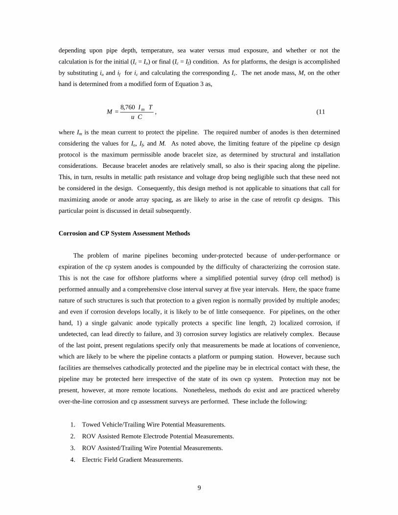
A reasonable approximation is that fc and ic exhibit a linear interdependence, as illustrated by Figure 5.

Thus,

f - f ic = corr c , (19

a

where fcorr is the free corrosion potential and a is the polarization resistance. Combining Equations 18 and

19 leads to an initial design expression for anode spacing as,

(fc - fa ) a � gLas = � ; (20

fcorr - fc 2p � rp � Ra

Table 2: Correspondence of the Coating Breakdown Factor and g to the percentage of bare area

and the corresponding a � g for a values of 20, 40, and 60 Ù � m 2 .

BARE AREA, %

COATING BREAKDOWN FACTOR

g ASSUMED a, W.m2

CORRESPONDING a.g, W.m2

0 0 ¥ - -

2 0.02 50 20 40 60

1,000 2,000 3,000

5 0.05 20 20 40

400 800

10 0.1 10

60 20 40 60

1,200 200 400 600

100 1 1 20 40 60

20 40 60

14

fcorr

a -

POT

EN

TIA

L

+

f a

CURRENT DENSITY

Figure 6: Proposed fc versus ic relationship with definition of a..

or, alternatively,

fcorr + (fa �y )f = , (21c

1 + y

where

a � gy = .

2p � rp � Las � Ra

The corresponding design life can be calculated from the modified version of Equation 3,

w � C � u T = . (22

8,760 � im � Ac( 1 )

Finally, upon combining Equations 17, 19, and 22,

w � C � u � a � gT = . (23

8,760 � (fcorr - fc ) � 2p � rp � Las

Since the term 2p � rp � Las � Ra / g (Equation 23) is equivalent to S (Equation 6), this approach is termed

15

the Slope Parameter Method for pipeline cp design. However, the magnitude of this slope parameter

differs from that of bare steel (12-15) by a factor of 1/g. On the basis that an upper limit of im for most

pipeline cp designs is 7 mA/ft2 (75 mA/m2) at fc = -0.80 VAg/AgCl, then a ‡ 2.0 W.m2. Considering further a

realistic upper limit for the coating breakdown factor as seven percent (g = 14.3) leads to a likely lower

limit value for a � g of 30 W � m 2 .

The initial step for a given design then is to calculate a baseline Las in terms of a.g, Ra (actually, anode

surface area or dimensions using, for example, McCoy’s formula (32)), and fc (design cathode potential)

using Equation 20. Upon substitution of this Las into Equation 23 and possibly with iteration via Equation

21 (such iteration may be necessary since anode dimensions and w are interrelated and changes in these, in

addition to changes in Las and a.g, result in a different fc and T, as calculated by Equation 23), w and T are

optimized.

Example Pipeline CP Design

Consider as an example the pipeline and cp design choices listed in Table 3. For these, and assuming

1) a standard 133 pound (60.8 kg) bracelet anode of length 1.42 ft (0.432 m) and outer radius 1.23 ft (0.187

m), fc = -0.975 VAg/AgCl (this constitutes a design polarized potential), and 3) Ra = 0.353 W as determined

from McCoy’s formula (32),

0.315 � r Ra = e , (24

Aa

where Aa is the anode surface area, then Equation 20 indicates Las = 170 m. From Equation 23, the

corresponding life is 30.1 years, which is consistent with the design requirement (Table 3). If these values

differ significantly, then iteration between Equations 20 and 23 based upon alternative choices for w (or

Ra), a, g, or Las (or for a combination of two or more of these terms) is required.

Table 3: Listing of pipe and electrolyte properties and design choices used in the example.

Pipeline Outer Radius, m 0.136 Pipeline Inner Radius, m 0.128

Electrolyte Resistivity, W � m 0.80

Alpha, 2W � m 7.5

Gamma 20 Design Life, years 30

Anode Current Capacity, Ah/kg 1,700 Anode Utilization Factor 0.8

Open Circuit Anode Potential, VAg/AgCl -1.05

16

This proposed method is considered to be an improvement upon the existing pipeline cp design

approach because, first, it is first principles based and not an algorithm as is the present method and,

second, of the additional parameters that it incorporates. Verification of the accuracy is presented

subsequently as is discussion demonstrating applicability of the equations upon which the approach is

based to retrofit cp situations.

TASK II: DEVELOPMENT OF AN INCLUSIVE, FIRST RPINCIPLES BASED ATTENUATION MODEL FOR MARINE PIPELINE CATHODIC PROTECTION

General

Limitations of the existing methods for modeling and analyzing potential attenuation along

cathodically polarized marine pipelines were discussed above. Briefly, these amount to the fact that the

Morgan/Uhlig approach does not incorporate anode resistance, whereas Boundary Element Modeling

excludes metallic path resistance. The newly proposed slope parameter based method for cp design for

new pipelines that was described in the preceding section also excludes metallic path resistance. With this

in mind, an attempt was made to derive a first principles based attenuation equation that incorporates all

four resistance terms (anode, coating, polarization, and metallic path resistances). This is presented in the

following section.

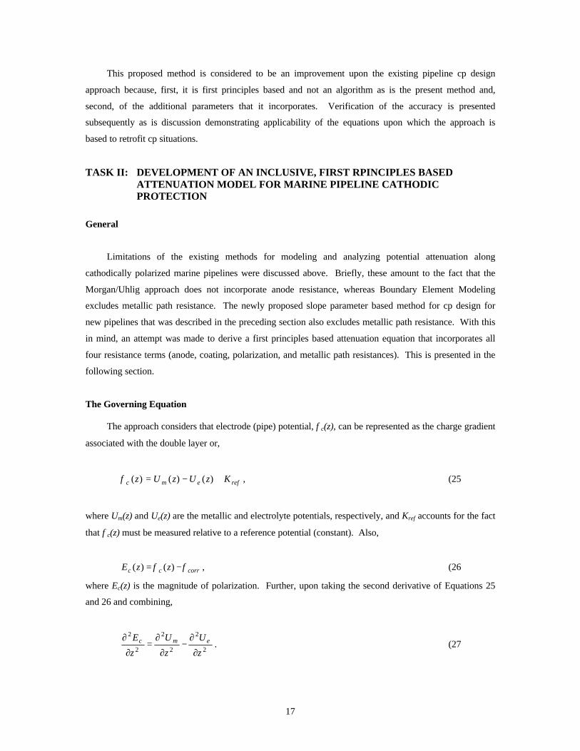
The Governing Equation

The approach considers that electrode (pipe) potential, fc(z), can be represented as the charge gradient

associated with the double layer or,

fc (z) = U m (z) - U e (z) + K ref , (25

where Um(z) and Ue(z) are the metallic and electrolyte potentials, respectively, and Kref accounts for the fact

that fc(z) must be measured relative to a reference potential (constant). Also,

Ec (z) = fc (z) -fcorr , (26

where Ec(z) is the magnitude of polarization. Further, upon taking the second derivative of Equations 25

and 26 and combining,

¶ 2 Ec ¶ 2U m ¶ 2U e= - . (27¶z 2 ¶z 2 ¶z 2

17

Expressions were then developed for each of the three component terms, Ec, Um, and Ue, and their second

derivatives, as described in the Appendix. These were substitution into Equation 27, which led to the

governing equation,

2¶

¶

E

zc 2

(z) +

¶E

¶ c

z

(z) � H �

Ł���

r

1

a

-1

z ł���

+ Ec (z) �Ł�� 2

z

H 2

- B ł��

= 2H � z

13

� � L

Ec (z * )dz* , (28 z

where ra is the radius of identical spherical anodes1 that are superimposed upon the pipe at intervals of 2L

and

r � rH = e p

andag

Rm � 2prpB = ,

ag

where re is electrolyte resistivity, The same linear relationship between fc and ic that was assumed in

development of Equations 20 and 23 (Figure 6) was employed here also. Because there is no known

solution to Equation 28, it must be solved numerically. This was done using an iterative, explicit finite

difference scheme that was based upon the first and second derivatives in space (33). The former was

represented by a backward finite difference given by,

dE E m+1 - E m+1

= i i-1 , (29dz dz

and the latter by,

d 2 E = i

m +1 i

m+1 im -1

+1

. (30 E - 2E + E

dz 2 dz 2

The integral term on the right hand side of Equation 28 was approximated using a trapezoidal summation

method as,

For mathematical simplicity, the model is based upon a spherical anode. Justification for thisassumption, given that actual anode are cylindrical bracelets is presented subsequently.

18

1

L

� � dz

2 ØŒº

m +1 m m m

N

m øœß

E(t)dt = E i + 2E i +1 + 2E i +2 .....+ 2EN -1 + E . (31 z

Substituting Equations 29, 30, and 31 into 28 yields,

Em

- 2Em +1 + E m +1 E m+1 - E m+1 H � 1 1 � � H �i +1 i i -1 i i-1 m+1

dz 2

+ dz

� 2 ��

Ł ra

-z �

�ł

+ Ei � ��Ł z 2

- B��ł

=

2H dz� � ØE i

m +1 + 2E im +1 + 2E i

m +2 .....+ 2EN

m -1 + E m ø , (32

z 3 2 μ N ϧ

which can be solved as,

H � dz ŒØ�� n-1

m ��

m Ͽ Ei

m -1

+1 � 1 1 � Eim -1

+1 Eim +1

z 3 �Œ�� 2Ei+ j � + En œ

+ dz

� H �� r

-z �� -

dz 2 -

dz 2

m+1 i ºŁ j =1 ł ß Ł a i ł Ei = , (33

- 2 H � 1 1 � � 2H � H � dz+ �� - �� + � + B� -

dz 2 dz Ł ra zi ł Ł z 2 ł zi 3

where n is the number of elements of length z. Equation 33 provides an explicit means to calculate the

cathode over-potential at each internal node for the next iteration step (m + 1) based on the present values

(iteration step ‘m’) at the nodes and their neighbors. The equations,

Ec ( z = 0 ) = fa -fcorr = Ea (34

and

dEc (z) = 0 , (35

dz

represent the boundary conditions at the end nodes; and the derivative boundary condition at the mid-anode

spacing is characterized by,

4 � E m+1 - E m+1

E m+1 = i=n-1 i=n-2 . (36i=n 3

The element closest to the anode, Ei=1, is assigned the value given by Equation 34, such that Ei=1 = Ea. As

an initial estimate is necessary for every element discretizing the cathode, a value for Ea is also assigned to

every element for the initial iteration step, m = 1. The iteration sequence was ended when the difference

19

between the root mean square value of the cathode over-potential for the present and previous iterations,

DErms, became less than 10-9.

True convergence of the model means that as dz approaches zero, the results from the finite difference

technique approach the true solution. In reality, the true solution is not known and is difficult to measure

in-situ; and so validity of the present model was judged based upon comparisons with an alternative

modeling technique (BEM) under conditions where this was considered acurate, as presented subsequently.

TASK III: VERIFICATION OF THE PROPOSED CATHODIC PROTECTION DESIGN METHOD AND ATTENUATION MODEL

Attenuation Equation

Figure 7 presents a plot of pipe potential as a function of distance from an anode as determined by 1)

Equation 14, 2) Boundary Element Modeling (BEM), and 3) the Finite Difference Method (FDM) solution

of Equation 28 for a � g values of 4, 20, 100, and 1,000 Ù � m2 (an a � g of 4 Ù � m2 corresponds to a

bare pipe with a current density demand of 100 mA/m2 at –1.05 VAg/AgCl, whereas an a � g of 1,000 Ù � m2

-1.10 Uhlig, ag = 1,000

Uhlig, ag = 4

BEM,FDM ag = 1,000

-1.00 ag = 100 BEM

FDM

BEM FDM

-0.90 ag = 20

BEM

ag = 8 FDM

-0.80

BEM -0.70

FDM ag = 4

0 20 40 60 80 100 120 140

DISTANCE, m

Figure 7: Potential as a function of distance for a pipeline protected by identical anodes spaced

244 m apart and with a � g values of 4, 8, 20, and 100 W � m2 .

POT

EN

TIA

L, V

(A

g/A

gCl)

20

-0.60

_________________________

corresponds, for example, to four percent bare area (g = 25) and a = 40 Ù � m 2 (current density demand

of 10 mA/m2 at –1.05 VAg/AgCl)). These a � g choices cover the range from a pipeline that is highly

difficult to polarize (a � g of 4 Ù � m 2 ) to one that should be typical of what is encountered in practice

(a � g of 1,000 Ù � m 2 ). Other pipe and electrolyte parameters are as listed in Table 4. For these

conditions, the solutions to Equation 14 are relatively insensitive to coating quality and current density

demand (a � g ) and are non-conservative compared to the BEM and Equation 28 results in that they predict

greater cathodic polarization. The Equation 28 and BEM potential profiles, on the other hand, are in good

mutual agreement. These are characterized by a potential decay within approximately the first 10 m of the

anode, the magnitude of which is determined by 1) anode resistance (dimensions and electrolyte resistivity)

and 2) the pipe current demand (a � g ). For each specific case, potential is relatively constant beyond the

range where anode resistance is influential and is defined by the voltage drop associated with the anode.

The finding that the FDM plateau potential is slightly more negative than the BEM one and that the

magnitude of this difference is inversely related to a � g is probably due to inclusion of the metallic path

resistance term in the former solution and its exclusion in the latter. However, the difference in the two

plateau potentials is not considered to be of practical significance. Because of the close correspondence

between the BEM and FDM results and because BEM is a proven methodology for quantitatively

characterizing potential fields, it is concluded that the FDM solution to Equation 28 is an appropriate means

for projecting potential attenuation along pipelines and anode current output.

As a further confirmation, Figure 8 presents attenuation profiles from 1) BEM, 2) the FDM solution

to Equation 28 with rm = 17 �10-8 W � m (the same as in Figure 7), and 3) the FDM solution to Equation 28

with rm = 0 for the same anode and pipe dimensions as for Figure 7 and ag = 100 W � m2 but for L = 3,000

Table 4: Pipe and electrolyte parameters for the analyses shown in Figure 7.

Pipeline Outer Radius, m 0.136

Pipeline Inner Radius, m 0.128

Anode Spacing, 2L, m 244

Equivalent Sphere Radius of Anode,2 m 0.201

Electrolyte Resistivity, W.m 0.30

Pipe Resistivity, W.m 17x10-8

Free Corrosion Pipe Potential, VAg/AgCl -0.65

Anode Potential, VAg/AgCl -1.05

This size corresponds to that of a standard 133 pound (60.8 kg) bracelet aluminum anode.

21

2

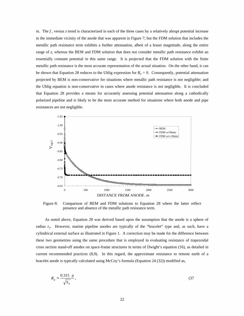
m. The fc versus z trend is characterized in each of the three cases by a relatively abrupt potential increase

in the immediate vicinity of the anode that was apparent in Figure 7; but the FDM solution that includes the

metallic path resistance term exhibits a further attenuation, albeit of a lesser magnitude, along the entire

range of z, whereas the BEM and FDM solution that does not consider metallic path resistance exhibit an

essentially constant potential in this same range. It is projected that the FDM solution with the finite

metallic path resistance is the most accurate representation of the actual situation. On the other hand, it can

be shown that Equation 28 reduces to the Uhlig expression for Ra = 0. Consequently, potential attenuation

projected by BEM is non-conservative for situations where metallic path resistance is not negligible; and

the Uhlig equation is non-conservative in cases where anode resistance is not negligible. It is concluded

that Equation 28 provides a means for accurately assessing potential attenuation along a cathodically

polarized pipeline and is likely to be the most accurate method for situations where both anode and pipe

resistances are not negligible.

-1.05

-1.00

-0.95

-0.90

-0.85

-0.80

-0.75

-0.70

-0.65

VA

gCl

BEM FDM w/Ohmic FDM w/o Ohmic

0 500 1000 1500 2000 2500 3000

DISTANCE FROM ANODE, m

Figure 8: Comparison of BEM and FDM solutions to Equation 28 where the latter reflect presence and absence of the metallic path resistance term.

As noted above, Equation 28 was derived based upon the assumption that the anode is a sphere of

radius ra. However, marine pipeline anodes are typically of the “bracelet” type and, as such, have a

cylindrical external surface as illustrated in Figure 1. A correction may be made for the difference between

these two geometries using the same procedure that is employed in evaluating resistance of trapezoidal

cross section stand-off anodes on space-frame structures in terms of Dwight’s equation (16), as detailed in

current recommended practices (8,9). In this regard, the approximate resistance to remote earth of a

bracelet anode is typically calculated using McCoy’s formula (Equation 24 (32)) modified as,

0.315 � r R » , (37a

Sa

22

where Sa is the exposed surface area of a cylindrical anode. By equating the surface area of the bracelet

anode to that of a sphere, the equivalent sphere radius, ra is calculated as,

Sa r » . (38a 4p

Anode current output can be determined from both BEM and the FDM solution of Equation 28, since

Ec(z) is proportional to current demand which, in turn, dictates Ia. Thus, Figure 9 presents a plot of Ia

versus ag, as determined by BEM, the FDM solution to Equation 28, and the Uhlig expression (Equation

14) based upon the same pipe and electrolyte parameters that were employed in conjunction with Figures 7

and 8. This reveals that results from the former two methods (BEM and FDM) are in excellent mutual

agreement, whereas Uhlig’s equation overestimates Ia in the lower ag range, presumably because of failure

of this expression to adequately address the near-field and the greater influence of the near-field at

relatively low ag. The Uhlig expression projects Ia with reasonable accuracy in cases where current

demand and coating quality are such that ag ‡ 100 W � m 2 . However, the BEM method is expected to

overestimate Ia also for 2L values for which metallic resistance is no longer negligible.

1 10 102 103 104

ALPHAxGAMMA, W.m2

Figure 9: Comparison of anode current output as projected by BEM, FDM, and Equation 14.

The results in Figures 7 and 8 indicate that a FDM solution to Equation 28 provides an accurate

projection of potential attenuation along a pipeline or riser and of anode current output. Because the

equation incorporates the electrolyte (anode), coating, and metallic resistance terms, it represents an

improvement over the Uhlig expression except in situations where electrolyte resistance is negligible and

over BEM where metallic path resistance is non-negligible.

10-2

10-1

1

10

102

FDM

BEM

Uhlig

23

Effect of Anode Spacing and Pipe Current Density Demand upon Potential Attenuation and Anode Current Output

Figures 10 and 11 present attenuation profiles for different one-half anode spacings from 200 to 3,000

m and a � g =100 W.m2 in the former case and for anode spacings from 100 to 10,000 m and a � g = 1,000

W.m2 in the latter. The same pipe and environment parameters in Table 4 apply here as well. These plots

-1.10

-1.00

VA

g/A

gCl

BEM FDM

-0.90 BEM FDM

-0.80 BEM BEMFDM

FDM BEM -0.70

FDM

-0.60 0 500 1000 1500 2000 2500 3000 3500

DISTANCE, m

Figure 10: Comparison of BEM and FDM potential profiles for pipelines with anode spacings

from 200 to 3,000 m and with a � g = 100W � m 2 .

-1.05

POT

EN

TIA

L, V

(A

g/A

gCl)

-0.95

-0.85

-0.75

-0.65

0 2000 4000 6000 8000 10000

DISTANCE, m

Figure 11: Comparison of BEM and FDM potential profiles for pipelines with anode spacings

from 100 to 10,000 m and with a � g = 1,000W � m 2 . The more negative profile for each pipe length is the BEM solution and the more positive the FDM.

24

indicate that the difference between the two analysis methods (BEM and Equation 28) increases with 1)

increasing distance from an anode, 2) increasing anode spacing, and 3) decreasing a � g . The FDM

solution is considered to be the more accurate of the two methods, at least for situations where metallic path

resistance is non-negligible. On this basis, situations can arise where BEM indicates protection along the

entirety of the pipeline but, in fact, under-protection exists beyond a certain distance. Accordingly,

Equation 28 is recommended as the analysis method of choice.

Figures 12 and 13 show plots of anode current output as a function of one-half anode spacing for the

same situations depicted in Figures 10 and 11, respectively. The BEM and FDM solutions are in good

agreement for relatively short spacings, but for greater ones the former projects that this current increases

0

500

1000

1500

2000

2500

3000

3500

mA

BEM FDM

0 500 1000 1500 2000 2500 3000 3500

HALF ANODE SPACING, m

Figure 12: Anode current output, as projected by BEM and Equation 28 (FDM), as a function of

half anode spacing and for a � g = 100W � m 2 .

25

Figure 13: Anode current output, as projected by BEM and Equation 28 (FDM), as a function of

half anode spacing and for 2000,1 m�W=� ga .

0

50

100

150

200

250

300

0 100 200 300 400 500 600 700 800 900 1000 HALF ANODE SPACING, m

mA

FDM BEM

progressively with increasing anode spacing whereas the FDM shows a maximum beyond which current

decreases. The latter effect is more pronounced in the lower a � g case. Again, this difference is

apparently due to BEM not including the metallic path resistance term. Also, the situations in Figures 10

0.05

0.04

0.03

0.02

0.01

0 0 200 400 600 800 1000 1200

ALPHAxGAMMA, Ohm.m2

and 11, where a more positive potential is projected by FDM than by BEM, correspond to the lower anode

current outputs in Figures 12 and 13.

Figure 14 presents a plot of potential difference between the BEM and the FDM solution to Equation

28, as shown graphically in Figures 10 and 11, at the mid-anode location as a function of ga � and for

various anode spacings from 50 to 10,000 m. This illustrates that, except for the shortest and greatest

anode spacings (50 and 10,000 m, respectively), the difference between the two potentials increases with

decreasing ga � . This is a consequence of Ia increasing with decreasing ga � such that a correspondingly

increasing voltage drop along the metallic path that was not accounted for in the BEM analysis resulted.

This trend was absent in the 2L = 50 m case because metallic path resistance is negligible for such a short

anode spacing at all ga � values considered. A reverse trend resulted for ga � values below about 600

2 m�W and 2L = 10,000 m. This apparently occurred because for these conditions polarization at the mid-

anode location was relatively small in both the FDM and BEM cases, and so the potential difference

between the two was small also.

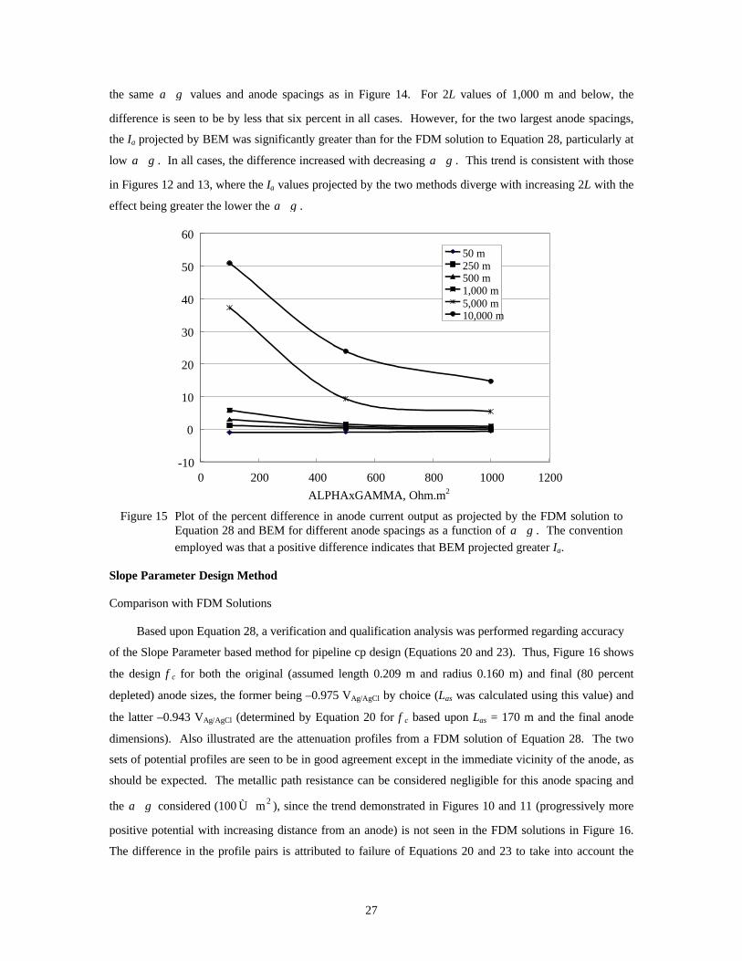
Figure 15 presents a plot of the percent difference in anode current output as a function of ga � for

0.06

0.07

MID

-AN

OD

E S

PAC

ING

POT

EN

TIA

L D

IFFE

RE

NC

E, V

50 m 250 m 500 m 1,000 m 5,000 m 10,000 m

Figure 14: Plot of the difference between the FDM solution to Equation 28 and BEM projections of pipe potential at the mid-anode location for different anode spacings as a function of a � g . The convention employed was that a positive difference indicates a more

negative projected potential via BEM.

26

-10

0

10

20

30

40

50

60

50 m 250 m 500 m 1,000 m 5,000 m 10,000 m

the same a � g values and anode spacings as in Figure 14. For 2L values of 1,000 m and below, the

difference is seen to be by less that six percent in all cases. However, for the two largest anode spacings,

the Ia projected by BEM was significantly greater than for the FDM solution to Equation 28, particularly at

low a � g . In all cases, the difference increased with decreasing a � g . This trend is consistent with those

in Figures 12 and 13, where the Ia values projected by the two methods diverge with increasing 2L with the

effect being greater the lower the a � g .

0 200 400 600 800 1000 1200

ALPHAxGAMMA, Ohm.m2

Figure 15 Plot of the percent difference in anode current output as projected by the FDM solution to Equation 28 and BEM for different anode spacings as a function of a � g . The convention employed was that a positive difference indicates that BEM projected greater Ia.

Slope Parameter Design Method

Comparison with FDM Solutions

Based upon Equation 28, a verification and qualification analysis was performed regarding accuracy

of the Slope Parameter based method for pipeline cp design (Equations 20 and 23). Thus, Figure 16 shows

the design fc for both the original (assumed length 0.209 m and radius 0.160 m) and final (80 percent

depleted) anode sizes, the former being –0.975 VAg/AgCl by choice (Las was calculated using this value) and

the latter –0.943 VAg/AgCl (determined by Equation 20 for fc based upon Las = 170 m and the final anode

dimensions). Also illustrated are the attenuation profiles from a FDM solution of Equation 28. The two

sets of potential profiles are seen to be in good agreement except in the immediate vicinity of the anode, as

should be expected. The metallic path resistance can be considered negligible for this anode spacing and

the a � g considered (100 Ù � m 2 ), since the trend demonstrated in Figures 10 and 11 (progressively more

positive potential with increasing distance from an anode) is not seen in the FDM solutions in Figure 16.

The difference in the profile pairs is attributed to failure of Equations 20 and 23 to take into account the

27

Condition Anode Current Output, A Difference, Equation 22 FDM Solution %

Initial (Anode Weight 60.8 kg) 0.214 0.221 -3.1 Final (Anode Weight 12.3 kg) 0.193 0.202 -4.4

VA

gCl

potential gradient near the anodes; however, this is thought to be within the uncertainty of the overall

process; and, hence, the results are considered acceptable. Table 5 lists the anode current output

determined by the two methods and indicates the difference to be relatively modest.

-1.10

-1.00

Equation 23 - Initial-0.90 FDM Results-Initial

Equation 23 - Final

FDM Results - Final

-0.80

0 10 20 30 40 50 60 DISTANCE FROM ANODE, m

Figure 16: Comparison of the results from the FDM solution to Equation 28 with the cathode potential used in the cp design based upon Equation 23.

Table 5: Anode current output as determined using a modified version of Equation 22 and the solution to Equation 28.

Range of Applicability of the Slope Parameter Design Approach

The proposed cp design approach based upon Equations 20 and 23 was evaluated by comparing the

results from it with the corresponding FDM solution to Equation 28. Thus, Figure 17 presents a plot of the

percent difference in fc at the mid-anode position (the location on the pipeline where polarization should be

least) as a function of the corresponding a.g that results from application of Equation 20 compared to what

is projected by the FDM solution to Equation 28 for the original anode and pipe dimensions in the above

example using different values of Las, and with re = 1.0 W.m. Only data for which a.g ‡ 30 W.m2 and fc £ ­

0.80 VAg/AgCl are included. In all cases, the error is less than three percent; and so any design that includes

the Las and a.g values indicated here and which also satisfies Equation 22 or 23 is considered acceptable.

28

-3%

-2%

-1%

0%

POT

EN

TIA

L E

RR

OR

- E

QU

AT

ION

21

Las = 10 m

Las = 50 m

Las = 100 m

Las = 200 m

Las = 400 m

Las = 800 m

10 100 1000 ALPHA*GAMMA(Ohm*m^2)

Figure 17: Error in polarized potential at the mid-anode position as determined from Equation 20 and referenced to the FDM solution to Equation 28 for re = 1.0 W.m.

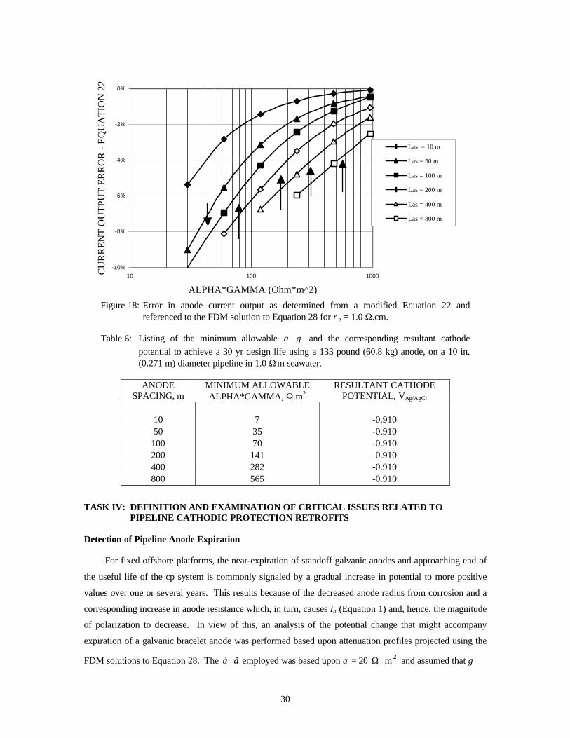
Relatedly, Figure 18 plots anode current output error versus a.g for the same conditions as in Figure 17

where a negative error indicates greater current output per the FDM solution than what is projected by

Equation 20. The percent error in current output at a particular a.g is greater than for potential (Figure 16)

but is still acceptable for most engineering applications. Similarly, for the same design parameters but with

a 0.15 W.m electrolyte, the maximum mid-spacing potential and anode current output errors are –1.5 and –

5.0 percent, respectively, which are less than for the 1.0 W.m electrolyte. In the latter case, an additional

calculation is necessary to confirm that adequate anode mass is available. Then, by resolving Equation 23

using defined values for all other parameters (C = 1700 Ah/kg and u =0.8), the minimum acceptable a.g for

anodes to achieve a 30 yr design life (that is, to maintain fc £-0.80 VAg/AgCl) was determined. The results of

this calculation, along with the corresponding fc values, as calculated iteratively using Equations 20 and 23,

are listed in Table 6 and are indicated for each Las in Figure 17 by an arrow (no arrow is shown for Las = 10

m since the minimum a.g for this anode spacing is below 30 W.m2). In the high a.g regime, the errors are

relatively small (the negative error indicates greater polarization according to the FDM solution compared

to Equation 23), they converge with increasing a.g, and order in proportion to anode spacing (larger error

the greater the anode spacing). The proposed design method has the advantage of providing an iterative

approach whereby different parameters, including anode spacing and cathode potential, can be optimized.

29

-10%

-8%

-6%

-4%

-2%

0%

CU

RR

EN

T O

UT

PUT

ER

RO

R -

EQ

UA

TIO

N 2

2

Las = 10 m

Las = 50 m

Las = 100 m

Las = 200 m

Las = 400 m

Las = 800 m

10 100 1000

ALPHA*GAMMA (Ohm*m^2)

Figure 18: Error in anode current output as determined from a modified Equation 22 and referenced to the FDM solution to Equation 28 for re = 1.0 W.cm.

Table 6: Listing of the minimum allowable a � g and the corresponding resultant cathode

potential to achieve a 30 yr design life using a 133 pound (60.8 kg) anode, on a 10 in. (0.271 m) diameter pipeline in 1.0 W.m seawater.

ANODE SPACING, m

MINIMUM ALLOWABLE ALPHA*GAMMA, W.m2

RESULTANT CATHODE POTENTIAL, VAg/AgCl

10 50

100 200 400 800

7 35 70

141 282 565

-0.910 -0.910 -0.910 -0.910 -0.910 -0.910

TASK IV: DEFINITION AND EXAMINATION OF CRITICAL ISSUES RELATED TO PIPELINE CATHODIC PROTECTION RETROFITS

Detection of Pipeline Anode Expiration

For fixed offshore platforms, the near-expiration of standoff galvanic anodes and approaching end of

the useful life of the cp system is commonly signaled by a gradual increase in potential to more positive

values over one or several years. This results because of the decreased anode radius from corrosion and a

corresponding increase in anode resistance which, in turn, causes Ia (Equation 1) and, hence, the magnitude

of polarization to decrease. In view of this, an analysis of the potential change that might accompany

expiration of a galvanic bracelet anode was performed based upon attenuation profiles projected using the

FDM solutions to Equation 28. The á � ã employed was based upon a = 20 W � m 2 and assumed that g

30

decreased with time because of coating deterioration according to the expression (9),

1 1 g = = . (39

f 0.07 + 0.004(T - 20)

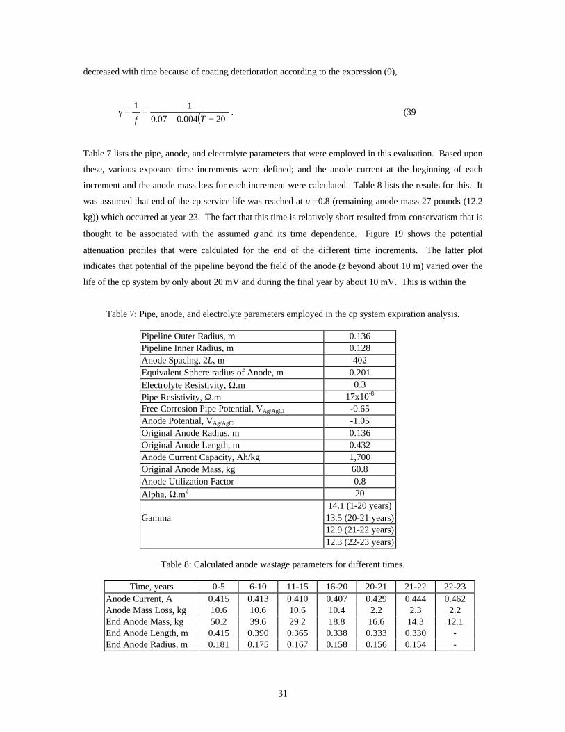
Table 7 lists the pipe, anode, and electrolyte parameters that were employed in this evaluation. Based upon

these, various exposure time increments were defined; and the anode current at the beginning of each

increment and the anode mass loss for each increment were calculated. Table 8 lists the results for this. It

was assumed that end of the cp service life was reached at u =0.8 (remaining anode mass 27 pounds (12.2

kg)) which occurred at year 23. The fact that this time is relatively short resulted from conservatism that is

thought to be associated with the assumed g and its time dependence. Figure 19 shows the potential

attenuation profiles that were calculated for the end of the different time increments. The latter plot

indicates that potential of the pipeline beyond the field of the anode (z beyond about 10 m) varied over the

life of the cp system by only about 20 mV and during the final year by about 10 mV. This is within the

Table 7: Pipe, anode, and electrolyte parameters employed in the cp system expiration analysis.

Pipeline Outer Radius, m 0.136 Pipeline Inner Radius, m 0.128 Anode Spacing, 2L, m 402 Equivalent Sphere radius of Anode, m 0.201 Electrolyte Resistivity, W.m 0.3 Pipe Resistivity, W.m 17x10-8

Free Corrosion Pipe Potential, VAg/AgCl -0.65 Anode Potential, VAg/AgCl -1.05 Original Anode Radius, m 0.136 Original Anode Length, m 0.432 Anode Current Capacity, Ah/kg 1,700 Original Anode Mass, kg 60.8 Anode Utilization Factor 0.8 Alpha, W.m2 20

14.1 (1-20 years) Gamma 13.5 (20-21 years)

12.9 (21-22 years) 12.3 (22-23 years)

Table 8: Calculated anode wastage parameters for different times.

Time, years 0-5 6-10 11-15 16-20 20-21 21-22 22-23 Anode Current, A 0.415 0.413 0.410 0.407 0.429 0.444 0.462 Anode Mass Loss, kg 10.6 10.6 10.6 10.4 2.2 2.3 2.2 End Anode Mass, kg 50.2 39.6 29.2 18.8 16.6 14.3 12.1 End Anode Length, m 0.415 0.390 0.365 0.338 0.333 0.330 -End Anode Radius, m 0.181 0.175 0.167 0.158 0.156 0.154 -

31

VA

g/A

gCl

-1.100-5 yrs5-10 yrs10-15 yrs

-1.05 15-20 yrs20-21 yr21-22 yr22-23 yr

-1.00

-0.95

-0.90

0 50 100 150 200 DISTANCE FROM ANODE, m

Figure 19: Potential attenuation profiles for a pipeline protected by galvanic bracelet anodes as a function of age.

range of normal variability and of measurement accuracy, and so it is concluded that insufficient pipe

depolarization accompanies anode wastage to disclose pending loss of protection. Lack of potential

sensitivity upon anode wastage resulted because the difference between the initial and final anode radii is

relatively small for the bracelet type of design.

Principle Design Parameters for Pipeline CP Retrofit

Although not necessarily recommended, one retrofit cp alternative in the case of platforms is one-to­

one replacement of the original stand-off anodes. Such an option is impractical for pipelines with galvanic

bracelets, however; and so other options must be considered. For these, the cost of ship and diver/ROV

time associated with anode installations along the pipeline are controlling and dictate that the guiding

principle for retrofit cp design should be maximization of the spacing between anodes so that as few

installations as possible are involved. An exception may arise, however, if geographical features of the

bottom terrain favor a lesser anode spacing.

The parameter of greatest significance for any marine cp design, including that for pipelines, is the

current density demand of the structure. Design values for new pipelines based upon bare surface area

were noted earlier as ranging from 60 to 220 mA/m2 depending upon pipe depth, temperature, and sea

water versus mud exposure (10). For Gulf of Mexico applications, a design value of about 20 mA/m2 (2

mA/ft2) based upon the coated surface area has historically been employed. In general, anode or anode

array size varies directly and spacing indirectly with magnitude of the design current density.

Consequently, the economic benefits to defining a design current density with minimal uncertainty and,

hence, without an unnecessarily high factor of safety (over-design) can be substantial. This is particularly

32

true for retrofits, although not necessarily for new construction, since in the latter case the material and

installation costs of bracelet anodes are a small fraction of the total project expense. For retrofits, however,

it is the number of anodes or anode array installations that is likely to be controlling, as noted above.

Pipeline Current Density Demand

As noted above, the á � ã term in Equations 20, 23, and 28 is, in effect, the pipe current density

demand; and two options have been identified for determining this parameter for existing pipelines based

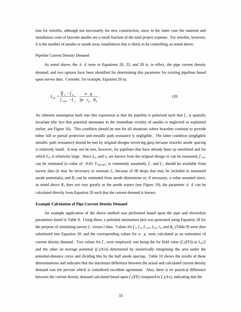
upon survey data. Consider, for example, Equation 20 as,

(f - f ) a � gLas = c a � . (20

fcorr - fc 2p � rp � Ra

An inherent assumption built into this expression is that the pipeline is polarized such that fc is spatially

invariant (the fact that potential attenuates in the immediate vicinity of anodes is neglected as explained

earlier, see Figure 16). This condition should be met for all situations where bracelets continue to provide

either full or partial protection and metallic path resistance is negligible. The latter condition (negligible

metallic path resistance) should be met by original designs involving gacp because bracelet anode spacing

is relatively small. It may not be met, however, for pipelines that have already been cp retrofitted and for

which Las is relatively large. Since Las and rp are known from the original design or can be measured, fcorr

can be estimated (a value of –0.65 VAg/AgCl is commonly assumed), fc and fa should be available from

survey data (it may be necessary to estimate fa because of IR drops that may be included in measured

anode potentials), and Ra can be estimated from anode dimensions or, if necessary, a value assumed since,

as noted above Ra does not vary greatly as the anode wastes (see Figure 19), the parameter á � ã can be

calculated directly from Equation 20 such that the current demand is known.

Example Calculation of Pipe Current Density Demand

An example application of the above method was performed based upon the pipe and electrolyte

parameters listed in Table 9. Using these, a potential attenuation plot was generated using Equation 28 for

the purpose of simulating survey fc versus z data. Values for fc, fa, fcorr, Las, rp, and Ra (Table 9) were then

substituted into Equation 20; and the corresponding values for a � g were calculated as an estimation of

current density demand. Two values for fc were employed, one being the far field value (fc(FF)) at Las/2

and the other an average potential (fc(Av)) determined by numerically integrating the area under the

potential-distance curve and dividing this by the half anode spacing. Table 10 shows the results of these

determinations and indicates that the maximum difference between the actual and calculated current density

demand was ten percent which is considered excellent agreement. Also, there is no practical difference

between the current density demand calculated based upon fc(FF) compared to fc(Av), indicating that the

33

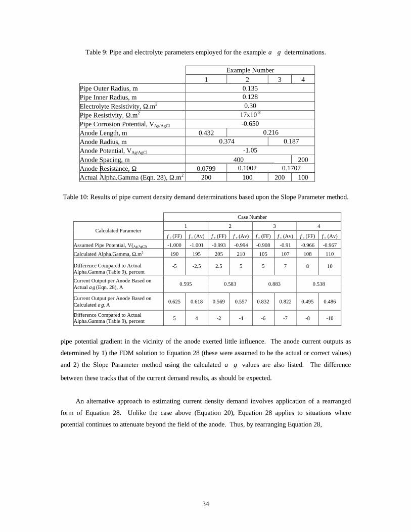
Table 9: Pipe and electrolyte parameters employed for the example a � g determinations.

Example Number 1 2 3 4

Pipe Outer Radius, m 0.135 Pipe Inner Radius, m 0.128

Electrolyte Resistivity, W.m2 0.30

Pipe Resistivity, W.m2 17x10-8

Pipe Corrosion Potential, VAg/AgCl -0.650 Anode Length, m 0.432 0.216 Anode Radius, m 0.374 0.187 Anode Potential, VAg/AgCl -1.05

Anode Spacing, m 400 200 Anode Resistance, W 0.0799 0.1002 0.1707 Actual Alpha.Gamma (Eqn. 28), W.m2 200 100 200 100

Table 10: Results of pipe current density demand determinations based upon the Slope Parameter method.

Case Number

Calculated Parameter 1 2 3 4

fc (FF) fc (Av) fc (FF) fc (Av) fc (FF) fc (Av) fc (FF) fc (Av)

Assumed Pipe Potential, V(Ag/AgCl) -1.000 -1.001 -0.993 -0.994 -0.908 -0.91 -0.966 -0.967

Calculated Alpha.Gamma, W.m2 190 195 205 210 105 107 108 110

Difference Compared to Actual Alpha.Gamma (Table 9), percent

-5 -2.5 2.5 5 5 7 8 10

Current Output per Anode Based on Actual ag (Eqn. 28), A

0.595 0.583 0.883 0.538

Current Output per Anode Based on Calculated ag, A

0.625 0.618 0.569 0.557 0.832 0.822 0.495 0.486

Difference Compared to Actual Alpha.Gamma (Table 9), percent 5 4 -2 -4 -6 -7 -8 -10

pipe potential gradient in the vicinity of the anode exerted little influence. The anode current outputs as

determined by 1) the FDM solution to Equation 28 (these were assumed to be the actual or correct values)

and 2) the Slope Parameter method using the calculated a � g values are also listed. The difference

between these tracks that of the current demand results, as should be expected.

An alternative approach to estimating current density demand involves application of a rearranged

form of Equation 28. Unlike the case above (Equation 20), Equation 28 applies to situations where

potential continues to attenuate beyond the field of the anode. Thus, by rearranging Equation 28,

34

-¶E

¶ (

z

z ) � r erp � (

r

1 -

1

z) - E( z ) � [

2r e

2

rp - Rm � 2p � rp ] +

2r e

3

rp �z

LE( t )dt z z

ag = a , (40¶ 2 E( z )

¶z 2

and then á � ã can be solved for based upon defining values for E(z) and the first and second derivatives

thereof (Equations 29 and 30, respectively) at selected z from survey data that indicate the potential profile.

As an evaluation of this approach, values for E(z), E’(z), and E”(z) for the attenuation profile that resulted

from cp for the same pipe and electrolyte parameters as in Table 4 but with á � ã = 200 W.m2 and Las = 200

m were measured at selected values for z. These z’s are necessarily near the anode because the potential

profile becomes flat beyond this and relatively large errors in the calculated E’ and E” are likely here.

Figure 20 shows the attenuation profile that was determined based upon Equation 28, and Table 11 lists the

results of the hind-sight á � ã calculation for five different z values using Equation 40. This shows that the

calculated values differ from the actual by from –25 to +61 percent. Such error is relatively large and

presumably resulted because E(z) varies sharply with z near the anode and minimally beyond about ten m.

This promotes error in one or more of the input potential parameters. The results do indicate, however, that

it should be possible to estimate á � ã within a factor of two. Note, however, that the error was minimal

(6.0 and 10.5 percent) at z = 4 and 5 m, respectively. With further study, it may be possible to identify an

ideal z at which á � ã should be estimated using this method.

Of the two methods (Slope Parameter (Equation 20) or FDM (Equation 40)), the former provided the

better accuracy; and so it is the recommended approach. If, however, attenuation persists beyond the field

of the anode, as should occur where pipe resistance is a factor, then the approach based upon Equation 40 is

0 20 40 60 80 100

Distance, m

Figure 20: Calculated attenuation profile.

-1.06

-1.05

-1.04

-1.03

-1.02

-1.01

-1.00

Pote

ntia

l, V

(A

g/A

gCl)

35

Table 11: Calculated parameters for the current density demand protocol.

z, m z Increment Potential, VAg/AgCl E(z), V E'(z) E''(z) ag Calculated Difference, %

0.9 i-1 -1.01630 1.0 i -1.01574 -0.3657 5.143E-03 -8.950E-03 322 61 1.1 i+1 -1.01527 2.9 i-1 -1.01213 3.0 i -1.01207 -0.3621 6.455E-04 -4.300E-04 239 19.5 3.1 i+1 -1.01200 3.9 i-1 -1.01162 4.0 i -1.01159 -0.3616 3.600E-04 -2.000E-04 212 6 4.1 i+1 -1.01155 4.9 i-1 -1.01132 5.0 i -1.01130 -0.3613 2.430E-04 -9.600E-05 221 10.5 5.1 i+1 -1.01128 6.9 i-1 -1.01100 7.0 i -1.01099 -0.361 1.075E-04 -5.000E-05 150 -25 7.1 i+1 -1.01098

the only alternative.

The above methods do not account for presence of residuals from the original anodes or exposed bare

steel portions of the bracelets. In effect, these serve as bare areas on the pipeline that will tend to drain the

cp current. Also, potential of any residual anodes, fa(residual), will probably be more positive than for the

retrofit anodes, fa(retrofit), in which case they will draw current also. Visual observations and potential

survey data should be helpful it defining this situation. If bare steel only is present, then the coating bare

area term, g, should be adjusted to reflect this and an overall current density demand calculated. For the

case where residuals from the original anodes are present, current demand should be less than for the steel-

only situation since the potential difference between these anodes and the new ones should be less than

when residuals are not present. In cases where the original anodes have corroded to a point where both

these and bare steel are present, a common mixed potential that is intermediate to both that of freely

corroding steel and of the residual anodes should be employed. On this basis, it can be reasoned that the

additional current that must be provided by the retrofit cp system because of an anode residual, Ib, is,

� fa ( retrofit ) - fa ( residual ) � Ib = (ic � Ar ) �

Ł��

fa ( retrofit ) ł�� , (41

where ic is the residual current density demand of the bare metal (steel or aluminum or a combination of the

two), and Ar is surface area of a residual. It can be assumed that ic for the residual aluminum is the same as

for steel. This approach assumes, however, that voltage drop associated with the bare areas is negligible,

36

which may not be the case. Boundary Element Modeling can provide insight into any limitations that

presence of bare metal might impose upon the proposed approach.

Anode/Anode Array Design

As noted above, the effect of 1) pipe current density demand, 2) anode/anode array design, and 3)

anode/anode array spacing is, in general, interrelated. Stated differently, it is current density demand and

anode/anode array resistance combined that determine the distance from an anode to which a pipeline is

protected. Consequently, optimization of the anode/anode array design is a key aspect in affecting an

efficient, effective retrofit cp system. If maximization of retrofit anode spacing is a design criterion, then

this translates to achieving as low a value for Ra as is practical. Equation 38 indicates that anode resistance

decreases in proportion to electrolyte resistivity and varies inversely with anode surface area. This

statement applies generally to all geometries and not just bracelets (17). Thus, influence of the former

parameter (resistivity) is such that anode arrays should be positioned above the mud bottom if at all

possible, since resistivity of mud is invariably greater than for sea water per se; and the support structure

(sled, for example) should be designed such that they remain so. In light of the surface area dependence of

anode resistance, the incentive for achieving low resistance is generally addressed by employing multiple

anodes (an array) with a common electrical connection to the pipeline rather than a single large anode (see

Equation 5). However, Equation 5 applies in situations where anodes are spaced sufficiently far apart that

interaction effects are negligible. Because it is impractical to widely separate anodes in most pipeline

retrofit anode array designs, interactions must be taken into account. Closed-form numerical solutions for

resistance of different configurations for multiple anodes are available in the literature (16-21); or,

alternatively, resistance can be calculated using BEM. Because the latter method can be expensive and

requires special training, numerical solutions are preferred for engineering practice. However, existing

resistance equations do not necessarily address likely configurations for pipeline retrofit anode arrays.

The case of non-interacting anodes (or at least anodes that are assumed not to interact) is relevant to

pipelines that receive protection from a platform to which they connect. In this regard, the equivalent

resistance spherical anode concept can be extended to this case by combining Equation 5 with the

expression for resistance of a spherical conductor to remote earth,

ra = r e , (42

4pRt

to yield

37

r e � N ra = . (43

4pRa

Figure 21 plots this radius versus N and shows that ra exceeds 50 m for a structure with 200 725 pound

(330 kg) anodes. Application of Equation 42, upon rearranging, to a 50 m diameter spherical anode

indicates its resistance in 0.15 W.m sea water to be 0.00048 W, which is approximately two orders of

magnitude less than for a single anode. Analyses have not yet been performed to determine the accuracy

with which the spherical anode concept can be applied in such situations and the extent to which a pipeline

can be protected by a platform.

0

10

20

30

40

50

60

Equ

ival

ent R

esis

tanc

e Sp

here

Rad

ius,

m

1 10 100 1000

Number of Anodes

Figure 21: Plot of the radius of a single, equivalent resistance spherical anode versus the number of actual anodes for the case where anodes do not interact.

Resistance determinations for situations where anodes do interact, as is likely to be the case for

retrofit anode arrays, can be made based upon the analysis proposed by Pierson and Hartt (34) for well

conductors, considering that n equal size anodes of length, l, and radius, r, where l >> r and N/4 is a whole

number, are arranged in a periodic square array. Here, the equivalent resistance of each group of four

contiguous anodes, R(4), is determined using Sunde’s equation for n parallel, deeply submerged, identical

electrodes spaced equally about the perimeter of a circle as,

R( N ) = 1 ØR1( r ) +

N �-1

R1(D sin(mp / N ))ø , (44N Œº m=1

ϧ

where D is diameter of the circle, and R1 and R1(Dsin[mp/m]) are generated from Sunde’s equation (17)

for resistance of a single, deeply submerged cylindrical electrode by the average potential method as,

38

Ø re ø ŒØ l�

Ł�1+ 1+ (r / l)2

�ł�

Ͽ

r )2R1 = Œ œ � Œln œ + - 1+ (r / l . (45º 2pl ß Œ r œ l

Œ œº ß

Thus, for four identical electrodes equally spaced about a circle, as shown in Figure 22, Equation 40

becomes,

RN 1

1( ) + [ (D sin( / 4) + R ( ) D ]. (46= [R r 2 R1 p ) 1 ]4

Also shown is the circumference of the single, equivalent resistance electrode. For values of n other than

four (but with n/4 still equaling a whole number), the process is repeated until a single electrode remains.

Anode (4)

D

Radius of a Single,

Equivalent Resistance

Anode

Figure 22: Schematic illustration of the equivalent resistance algorithm for a square array of four electrodes.

A more general situation, however, is that of a rectangular array for which n/4 is not necessarily a

whole number. Here, the equivalent resistance, Rn, can be estimated by a sequential calculation, the first

step of which involves Sunde’s equation (17) for the equivalent resistance of a deeply submerged, linear

array of identical electrodes spaced a distance s apart as,

RN 1

��

R ( ) + 2 [(N -1 R ( ) ( N - 2)R ( s)+ �� � + R ( � = 1 r ) 1 s + 1 2 1 Ns - s)]� . (47

N Ł N ł

and its equivalent resistance determined. Next, the equivalent resistance of each row is calculated; and

each row is replaced by a single electrode, the radius of which corresponds to this equivalent resistance.

39

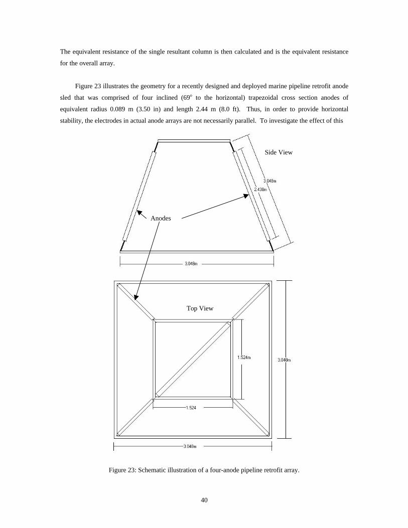
The equivalent resistance of the single resultant column is then calculated and is the equivalent resistance

for the overall array.

Figure 23 illustrates the geometry for a recently designed and deployed marine pipeline retrofit anode

sled that was comprised of four inclined (69o to the horizontal) trapezoidal cross section anodes of

equivalent radius 0.089 m (3.50 in) and length 2.44 m (8.0 ft). Thus, in order to provide horizontal

stability, the electrodes in actual anode arrays are not necessarily parallel. To investigate the effect of this

Side View

Top View

Anodes

Figure 23: Schematic illustration of a four-anode pipeline retrofit array.

40

non-parallelism, equivalent resistance of the array was calculated using, first, Equation 43 assuming the

electrodes are parallel and, second, BEM based upon the actual (inclined) configuration. In the former

case, Rn = 0.0233 W and in the latter 0.0237 W, such that the difference between the two equivalent

resistances is less than two percent. The corresponding equivalent spherical radius is 1.137 m.

The resistance of the array in Figure 23 decreases as either the number or size of the anodes increases

(or both). For example, Table 12 lists the resistance of the same sled as above but with 725 pound (330 kg)

anodes (equivalent radius 0.52 ft (0.159 m)). Also included is resistance of a 16 725 pound (330 kg) square

pattern array with anodes spaced at two m (center-to-center). This indicates that, in addition to the

Equation 42 and BEM results being in good mutual agreement, the resistance decrease associated with

increased anode sizing is relatively modest but that the 4x4 array resistance is about one-half that of the

2x2.

Table 12: Resistance of different anode arrays.

Array Type Resistance (BEM), Ohms Resistance (Eqn. 41), Ohms

2x2 4x4

0.021 0.0112

0.021 0.0119

Maximized Anode/Anode Array Spacing

Either of two approaches can be taken to optimize anode/anode array spacing. The first of these is

relevant when the pipeline terminates at and receives cathodic protection from a relatively large structure.

Equation 5 indicates that anode resistance for such situations is very low provided N is sufficiently large, in

which case the Uhlig/Morgan equation (Equation 14) applies. This expression can also be used in non-zero

anode resistance situations provided the potential at the drainage (electrical connection) point, Ea in

Equation 14 and Figure 1, is known. If the pipeline is at “remote earth” relative to the platform, then a

closed form numerical solution can be used to calculate anode resistance and voltage drop. In this case,

pipe potential at the drainage point, Ea, equals the potential at the anode surface minus this voltage drop.

Alternatively, BEM can by employed, irrespective of whether or not the anode/anode array is positioned

remotely from the pipeline.

Accuracy of the above type of anode/anode array resistance modeling may be limited, however, if a

portion of the pipe is positioned within the radius of the equivalent resistance anode. Alternatively, the

pipeline may be positioned within the potential field of one or more anodes of the array despite its being

remote with respect to the field of the equivalent resistance anode.

41

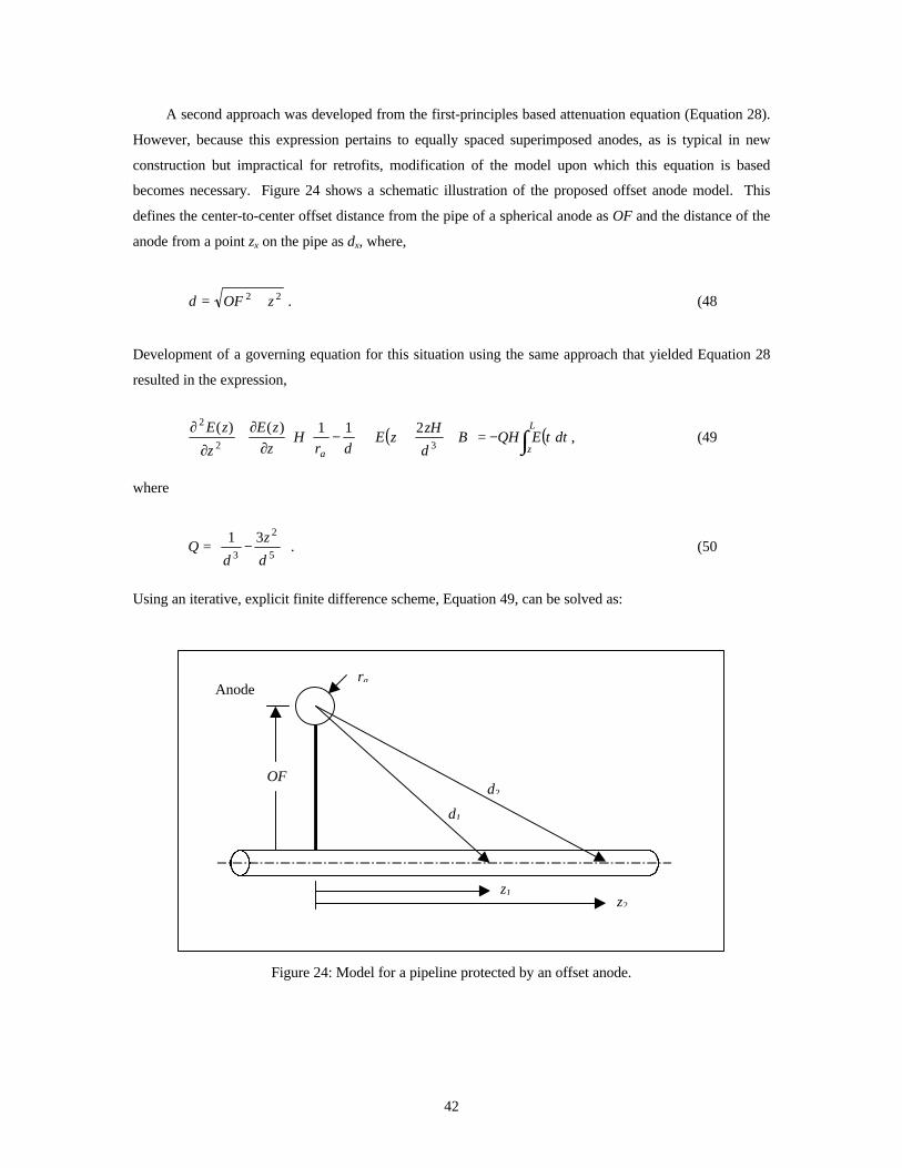
22 zOFd +=

A second approach was developed from the first-principles based attenuation equation (Equation 28).

However, because this expression pertains to equally spaced superimposed anodes, as is typical in new

construction but impractical for retrofits, modification of the model upon which this equation is based

becomes necessary. Figure 24 shows a schematic illustration of the proposed offset anode model. This

defines the center-to-center offset distance from the pipe of a spherical anode as OF and the distance of the

anode from a point zx on the pipe as dx, where,

. (48

Development of a governing equation for this situation using the same approach that yielded Equation 28

resulted in the expression,

¶ 2 E(z) ¶E(z) � 1 1 � Ø 2zH ø L

2 � H �� - �� + ( ) � Œ 3

+ Bœ = -QH � E( ) t dt ,+ E z (49¶z ¶z Ł ra d ł º d ß z

where

Q = ��� 1

3 -

3z 5

2

���

. (50 Ł d d ł

Using an iterative, explicit finite difference scheme, Equation 49, can be solved as:

ra Anode

OF

d1

d2

z1 z2

Figure 24: Model for a pipeline protected by an offset anode.

42

- QHdz �� N -1

2E m + E m �� Ei

m -1

+1

H ��� 1

-1 �

�� -Ei

m -1

+1

-Ei

m +1� i+ j N � +

2 � dz Ł ra d i ł dz 2 dz 2 m+1 Ł j =1 łEi = . (51

- 2 +

H ��� 1

-1 �

�� +�� 2zi H

+ B ��� +

QHdz 2 3dz dz Ł ra d i ł �

Ł di ł 2

Equation 28 assumes the potential of the pipe element closest to the anode to be the same as for the anode.

However, in the offset case, these potentials are different. Defining pipe potential at the drainage point was

accomplished by, first, calculating the anode current output for the case where this electrode is

superimposed upon the pipe (Equation 28) using a FORTRAN/FDM program and, second, calculating

potential drop in the electrolyte from the expression,

re I Ø 1 1 øDfra fiOF = Œ - œ . (52

4p º ra OF ß

The pipe potential at z = 0 for the offset anode configuration can then estimated as,

fc (z = 0) = fa - Dfra fiOF . (53

This value is inputted to an iterative FORTRAN/FDM program and Equation 51 solved. The model was

tested using the same parameters as for the earlier examples except with ra = 0.170 m, re = 0.15 and 1.0

W.m, á � ã values of 100 and 1,000 W.m2, Las = 200, 500, 750, 1,000, and 2,000 m, and OF = 1, 5, and 10

m. The example is not realistic with regard to a retrofit situation, however, because of the small anode size.

Voltage drop through the anode connection cable was assumed to be negligible.

Figures 25-27 show attenuation profiles for each of the three offset distances, re = 0.15, á � ã = 100

W.m2, and anode spacings of 200, 500, 750, 1,000, and 2,000 m in comparison to results from a companion

BEM analysis, where the latter employed a cylindrical anode of the same equivalent resistance as the FDM

one. This water resistivity (re = 0.15 W.m) is considered to approach the lower limit of what is likely to be

encountered in practice. The results indicate, first, that the BEM projects greater cathodic polarization than

does the FDM solution to Equation 51 with magnitude of the difference increasing in proportion to anode

spacing. This reflects, at least in part, the fact that the BEM analysis neglects metallic path resistance as

discussed above. Second, potential at z = 0 is progressively more positive the greater the offset distance.

Note, however, that the far field potential is virtually independent of the offset. Also, while these offset

anodes provide protection at a spacing of 2,000 m and probably slightly beyond, the protection distance

afforded by superimposed bracelets is less (see Figure 10). This difference presumably occurred because

with the offset less current was delivered to the pipe in the immediate vicinity of the anode, and so more

43

-0.65

-0.75 PO

TE

NT

IAL

, VA

g/A

g/C

lFDM

BEM -0.825

-0.85 -0.862

-0.905

-0.928 -0.932

-0.95 -0.963 -0.951 -0.979

-1.011

-1.020

-1.05

0 200 400 600 800 1000

DISTANCE, m

Figure 25: Attenuation plots for a 0.271 m (nominal 10 in) diameter pipeline with re = 0.15 W.m, á � ã = 100 W.m2, and a 0.340 m diameter spherical anode offset at one m.

-0.65

POT

EN

TIA

L, V

Ag/

AgC

l

FDM

-0.75 BEM

-0.826

-0.85

-0.862

-0.905

-0.928 -0.932

-0.95 -0.963 -0.951-0.979

-1.011 -1.020

-1.05

0 200 400 600 800 1000

DISTANCE, m

Attenuation plots for a 0.271 m (nominal 10 in) diameter pipeline with re = 0.15 W.m,Figure 26: á � ã = 100 W.m2, and a 0.340 m diameter spherical anode offset at five m.

current was available at distant locations.

Correspondingly, Figures 28-30 show companion plots to the ones in Figures 25-27 but for á � ã =

1,000 W.m2. The trends in the two sets of plots are similar except that 1) attenuation is less in the

immediate vicinity of the anode, 2) protection of the pipe is affected at a more negative potential, and 3)

44

-0.65

FDM -0.75

BEM-0.826

-0.85-0.862

-0.905

-0.928-0.931

-0.95-0.963 -0.951

-0.979

-1.010

-1.020

-1.05

0 200 400 600 800 1000

DISTANCE, m

Figure 27: Attenuation plots for a 0.271 m (nominal 10 in) diameter pipeline with re = 0.15 W.m,

POT

EN

TIA

L, V

Ag/

AgC

l

á � ã = 100 W.m2, and a 0.340 m diameter spherical anode offset at ten m.

-1.00

-1.007

-1.02-1.020

-1.028

-1.034-1.036

POT

EN

TIA

L, V

Ag/

AgC

l

-1.039 -1.040-1.04 FDM -1.044

-1.046 BEM-1.050

-1.06

0 200 400 600 800 1000

DISTANCE, m

Attenuation plots for a 0.271 m (nominal 10 in) diameter pipeline with re = 0.15 W.m,Figure 28: á � ã = 1,000 W.m2, and a 0.340 m diameter spherical anode offset at one m.

45

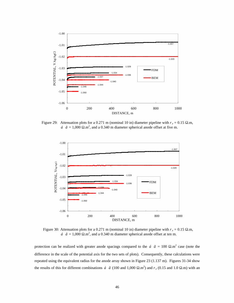
POT

EN

TIA

L, V

Ag/

AgC

l

Figure 29:

-1.00

-1.01 -1.007

-1.02-1.020

-1.029-1.03

FDM -1.034

-1.036-1.037 BEM

-1.04-1.040

-1.044-1.046

-1.05 -1.050

-1.06

0 200 400 600 800 1000DISTANCE, m

Attenuation plots for a 0.271 m (nominal 10 in) diameter pipeline with re = 0.15 W.m, á � ã = 1,000 W.m2, and a 0.340 m diameter spherical anode offset at five m.

-1.00

-1.007

-1.01

-1.02-1.020

-1.028-1.03

-1.034 FDM-1.036

-1.039-1.04 -1.040

-1.044 BEM-1.046

-1.05 -1.050

-1.06

0 200 400 600 800 1000DISTANCE, m

Figure 30: Attenuation plots for a 0.271 m (nominal 10 in) diameter pipeline with re = 0.15 W.m,

POT

EN

TIA

L, V

Ag/

AgC

l

á � ã = 1,000 W.m2, and a 0.340 m diameter spherical anode offset at ten m.

protection can be realized with greater anode spacings compared to the á � ã = 100 W.m2 case (note the

difference in the scale of the potential axis for the two sets of plots). Consequently, these calculations were

repeated using the equivalent radius for the anode array shown in Figure 23 (1.137 m). Figures 31-34 show

the results of this for different combinations á � ã (100 and 1,000 W.m2) and re (0.15 and 1.0 W.m) with an

46

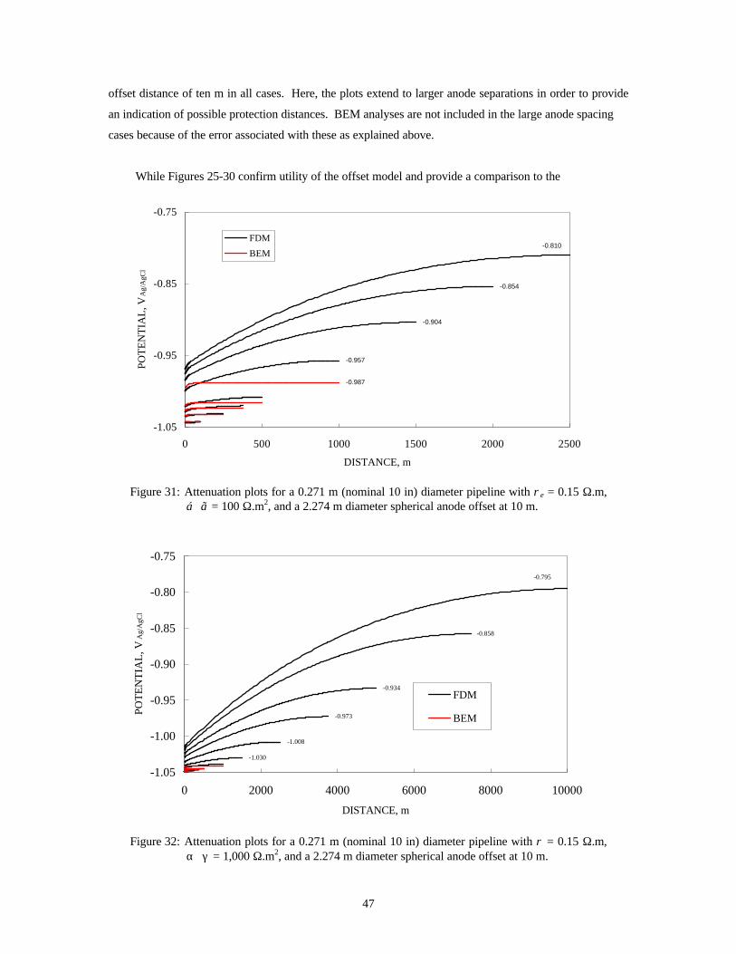
offset distance of ten m in all cases. Here, the plots extend to larger anode separations in order to provide

an indication of possible protection distances. BEM analyses are not included in the large anode spacing

cases because of the error associated with these as explained above.

While Figures 25-30 confirm utility of the offset model and provide a comparison to the

-0.75

FDM -0.810

BEM

POT

EN

TIA

L, V

Ag/

AgC

l

-0.85 -0.854

-0.904

-0.95 -0.957

-0.987

-1.05

0 500 1000 1500 2000 2500

DISTANCE, m

Figure 31: Attenuation plots for a 0.271 m (nominal 10 in) diameter pipeline with re = 0.15 W.m, á � ã = 100 W.m2, and a 2.274 m diameter spherical anode offset at 10 m.

-0.75

-0.795

-0.80

-0.85 -0.858

-0.90

-0.934

-0.95 FDM

-0.973 BEM

POT

EN

TIA

L, V

Ag/

AgC

l

-1.00 -1.008

-1.030

-1.05

0 2000 4000 6000 8000 10000

DISTANCE, m

Figure 32: Attenuation plots for a 0.271 m (nominal 10 in) diameter pipeline with r = 0.15 W.m, a � g = 1,000 W.m2, and a 2.274 m diameter spherical anode offset at 10 m.

47

POT

EN

TIA

L, V

Ag/

AgC

l

-0.65

-0.697

-0.75 -0.767

-0.820

-0.85

FDM -0.95

BEM

-1.05 0 500 1000 1500 2000 2500

DISTANCE, m

Figure 33: Attenuation plots for a 0.271 m (nominal 10 in) diameter pipeline with r = 1.0 W.m, a � g = 100 W.m2, and a 2.274 m diameter spherical anode offset at 10 m.

-0.80

-0.849

-0.85

POT

EN

TIA

L, V

Ag/

AgC

l

-0.894-0.90

-0.943 FDM-0.95

BEM

-0.984

-1.00 -1.005

-1.05 0 1000 2000 3000 4000 5000

DISTANCE, m

Figure 34: Attenuation plots for a 0.271 m (nominal 10 in) diameter pipeline with r = 1.0 W.m, a � g = 1,000 W.m2, and a 2.274 m diameter spherical anode offset at 10 m.

superimposed anode case (Figures 7, 10, and 11), the physical situation is probably not relevant to a cp

retrofit because of the small anode size that was involved (spherical anode with radius 0.170 m).

Consequently, these calculations were repeated using the equivalent radius for the anode array shown in

Figure 23 (1.137 m). Figures 31-34 show the results of this for different combinations á � ã (100 and 1,000

48

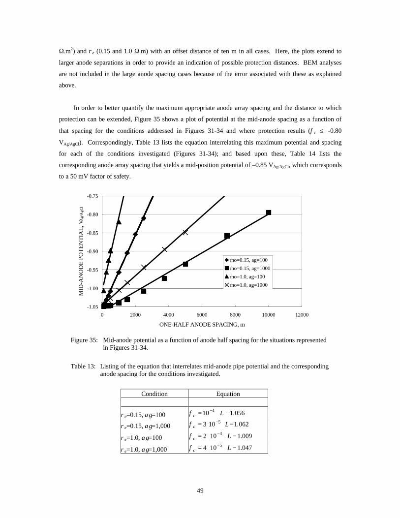
W.m2) and re (0.15 and 1.0 W.m) with an offset distance of ten m in all cases. Here, the plots extend to

larger anode separations in order to provide an indication of possible protection distances. BEM analyses

are not included in the large anode spacing cases because of the error associated with these as explained

above.

In order to better quantify the maximum appropriate anode array spacing and the distance to which

protection can be extended, Figure 35 shows a plot of potential at the mid-anode spacing as a function of

that spacing for the conditions addressed in Figures 31-34 and where protection results (fc £ -0.80

VAg/AgCl). Correspondingly, Table 13 lists the equation interrelating this maximum potential and spacing

for each of the conditions investigated (Figures 31-34); and based upon these, Table 14 lists the

corresponding anode array spacing that yields a mid-position potential of –0.85 VAg/AgCl, which corresponds

to a 50 mV factor of safety.

-1.05

-1.00

-0.95

-0.90

-0.85

-0.80

-0.75

MID

-AN

OD

E P

OT

EN

TIA

L, V

Ag/

AgC

l

rho=0.15, ag=100

rho=0.15, ag=1000

rho=1.0, ag=100

rho=1.0, ag=1000

0 2000 4000 6000 8000 10000 12000

ONE-HALF ANODE SPACING, m

Figure 35: Mid-anode potential as a function of anode half spacing for the situations represented in Figures 31-34.

Table 13: Listing of the equation that interrelates mid-anode pipe potential and the corresponding anode spacing for the conditions investigated.

Condition Equation

re=0.15, ag=100

re=0.15, ag=1,000

cf

cf

1 05610 4 .L -�= -

1 0623 10 5 .L -��= -

re=1.0, ag=100 cf 1 0092 10 4 .L -��= -

re=1.0, ag=1,000 cf 1 0474 10 5 .L -��= -

49

Table 14: Listing of projected maximum anode array spacings that result in a mid-anode potential of –0.85 VAg/AgCl.

Water/Mud Resistivity, W.m

ag, W.m2

Approximate Bracelet Anode Spacing (Figs. 10 and 11), m

Approximate Retrofit Anode Array Spacing (Fig. 35), m

0.30 0.30 0.15 0.15 1.00 1.00

100 1,000 100

1,000 100

1,000

1,500 8,000

----

--

4,100 14,100 1,600

10,000

TASK V: RECOMMENDED PROTOCOL FOR RETROFIT CATHODIC PROTECTION DESIGN OF MARINE PIPELINES

Figure 36 presents a flow diagram that overviews the pipeline cp retrofit decision and design process.

The critical features here are listed as follows:

1. Determination that a cp retrofit is required.

2. Determination of pipe current density demand and, hence, of the required anode current output.

3. Determination of whether anode array spacing is to be governed by factors such 1) terrain or proximity to shore or structure(s) or 2) minimization of the number of anode arrays.

4. Anode array design.

Candidate protocols and methods for addressing each of these are presented under Task IV above.

50

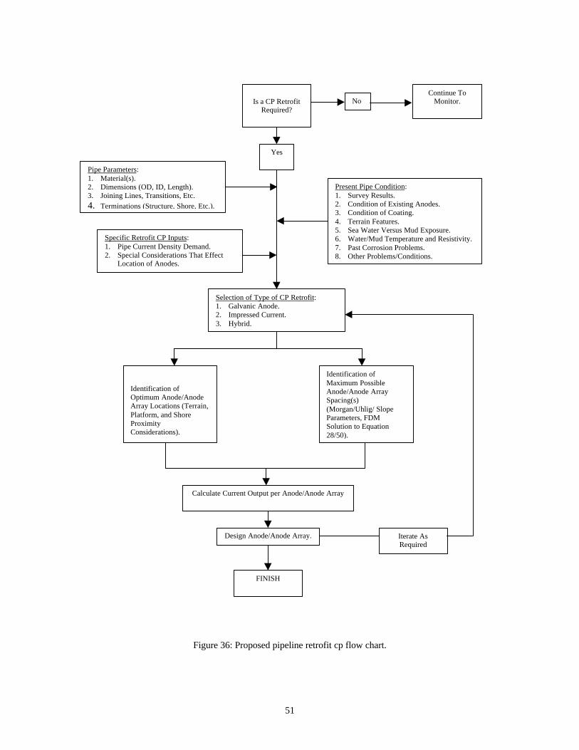
No Continue To

Monitor.Is a CP RetrofitRequired?

Pipe Parameters: 1. Material(s).

Present Pipe Condition:2. Dimensions (OD, ID, Length). 1. Survey Results.3. Joining Lines, Transitions, Etc. 2. Condition of Existing Anodes.4. Terminations (Structure, Shore, Etc.). 3. Condition of Coating. 4. Terrain Features. 5. Sea Water Versus Mud Exposure.

Specific Retrofit CP Inputs: 6. Water/Mud Temperature and Resistivity. 1. Pipe Current Density Demand. 7. Past Corrosion Problems. 2. Special Considerations That Effect 8. Other Problems/Conditions.

Location of Anodes.

Yes

Selection of Type of CP Retrofit: 1. Galvanic Anode. 2. Impressed Current. 3. Hybrid.

Identification of Maximum Possible Anode/Anode Array Spacing(s) (Morgan/Uhlig/ Slope Parameters, FDM Solution to Equation 28/50).

Calculate Current Output per Anode/Anode Array

Design Anode/Anode Array. Iterate As Required

Identification of Optimum Anode/Anode Array Locations (Terrain, Platform, and Shore Proximity Considerations).

FINISH

Figure 36: Proposed pipeline retrofit cp flow chart.

51

BIBLIOGRAPHY

1. T. Andersen and A. Misund, “Pipeline Reliability: An Investigation of Pipeline Failure Characteristics and Analysis of Pipeline Failure Rates for Submarine and Cross-Country Pipelines,” J. Pet. Technology, April, 1983, p. 709.

2. “Analysis of the MMS Pipeline Leaks Report for the Gulf of Mexico, Texaco USA, 133 W. Santa Clara, Ventura, CA 93001, October 25, 1985.

3. J. S. Mandke, “Corrosion Causes Most Pipeline Failures in the Gulf of Mexico, Oil and Gas Journal, October 29, 1990, p. 40.

4. “Improving the Safety of Marine Pipelines,” Committee on the Safety of Marine Pipelines, Marine Board, National Research Council, Washington, D.C., 1994.

5 Minerals Management Service Data Base, Gulf of Mexico Region, New Orleans, LA.

6 C. Weldon and D. Kroon, “Corrosion Control Survey Methods for Offshore Pipelines,” Proceedings International Workshop on Offshore Pipeline Safety, New Orleans, Dec. 4-6, 1991, p. 196.

7. ‘International Workshop on Corrosion Control for Marine Structures,” Eds: G.R.Edwards, W. Hanzalek, S. Liu, D.L. Olson, and C. Smith, Am Bureau of Shipping, Houston, 2000.

8. J. Britton, “Continuous Surveys of Cathodic Protection System performance on Buried Pipelines in the Gulf of Mexico,” paper no. 422 presented at CORROSION/92, Nashville, April 26-30, 1992.

9. "Corrosion Control of Steel-Fixed Offshore Platforms Associated with Petroleum Production", NACE Standard RP 0176, NACE, Houston, 1976.

10. “Cathodic Protection Design,” DnV Recommended Practice RP401, Det Norske Veritas Industri Norge AS, 1993.

11. "Corrosion Control of Steel-Fixed Offshore Platforms Associated with Petroleum Production", NACE Standard RP 0176, NACE, Houston, 1976.

12. Wang, W., Hartt, W. H., and Chen, S., Corrosion, vol. 52, 1996, p. 419.

13. W. H. Hartt, Chen, S., and Townley, D. W., Corrosion, vol. 54, 1998, p 317.

14. Townley, D. W., “Unified Design Equation for Offshore Cathodic Protection,” paper no. 97473 presented at CORROSION/97, March 9-14, 1997, New Orleans.

15. “Design of Galvanic Anode Cathodic Protection Systems for Offshore Structures,” NACE International Publication 7L198, NACE International, Houston, TX, 1998.

16. Dwight, H. B., Electrical Engineering, Vol. 55, 1936, p. 1319.

17. Sunde, E. D., Earth Conduction Effects in Transmission Systems, Dover Publications, Inc., New York, 1968.

18. McCoy, J. E., Transactions Institute of Marine Engineers, Vol. 82, 1970, p. 210.

19. Cochran, J. C., “A Correlation of Anode-to-Electrolyte Resistance Equations Used in Cathodic Protection,” paper no. 169 presented at CORROSION/82, March 22-26, 1982, Houston.

52

20. Strommen, R., Materials Performance, Vol. 24(3), 1985, p. 9.

21. Cochran, J. C., “Additional Anode-to-Electrolyte Resistance Equations Useful in Offshore Cathodic Protection,” paper no. 254 presented at CORROSION/84, April 2-6, 1984, New Orleans.

22. Foster, T., and Moores, V. G., “Cathodic Protection Current Demand of Various Alloys in Sea Water,” paper no. 295 presented at CORROSION/86, March 17-2, 1986, Houston.

23. Mollan, R. and Anderson, T. R., “Design of Cathodic Protection Systems,” paper no. 286 presented at CORROSION/86, March 17-2, 1986, Houston.

24. Fischer, K. P., Sydberger, T. and Lye, R., “Field Testing of Deep Water Cathodic Protection on the Norwegian Continental Shelf,” paper no. 67 presented at CORROSION/87, March 9-13, 1987, San Francisco.

25. Fischer, K. P. and Finnegan, J. E., “Cathodic Protection Behavior of Steel in Sea Water and the Protective Properties of the Calcareous Deposits,” paper no. 582 presented at CORROSION/89, April 17-21, 1989, New Orleans.

26. Schrieber, C. F. and Reding, J., “Application Methods for Rapid Polarization of Offshore Structures,” paper no. 381 presented at CORROSION/90, April 23-27, 1990, Las Vegas.

27. Burk, J. D., “Dualnode Field Performance Evaluation – Cathodic Protection for Offshore Structures,” paper no. 309 presented at CORROSION/91, March 11-14, 1991, Cincinnati.

28. “Pipeline Cathodic Protection – Part 2: Cathodic Protection of Offshore Pipelines,” Working Document ISO/TC 67/SC 2 NP 14489, International Standards Organization, May 1, 1999.

29. Morgan, J., Cathodic Protection, Macmillan, New York, 1960, pp. 140-143.

30. Uhlig, H. H. and Revie, R. W., Corrosion and Corrosion Control, Third Edition, John Wiley and Sons, New York, 1985, p. 223.

31. Strommen, R. and Rodland, A, Materials Performance, Vol. 20 No. 10, 1981, p. 7.

32. McCoy, J. E., “Corrosion Control by Cathodic Protection – Theoretical and Design Concepts for Marine Applications”, The Institute of Marine Engineers Transactions, Vol. 82, 1970, p. 210.

33. Chapra, C. S. and Canale, R. P., Numerical Methods for Engineers, McGraw-Hill, Second Ed., New York, 1988, pp. 734-737.

34. P. Pierson and W. H. Hartt, “Galvanic Anode Cathodic Polarization of Steel in Sea Water: Part IV – Conductor Arrays on Petroleum Production Platforms,” Corrosion, Vol. 55, 1999, p. 686.

53

APPENDIX A

Derivation of the First-Principles Pipeline Attenuation Equation

54

Generalized Formulation

Electrode potential (pipe or riser potential in this case), fc(z), can be represented as the charge

gradient associated with a double layer or

fc ( z ) = U m ( z ) - U e ( z ) + K ref , (A1

where Um(z) and Ue(z) are the metallic and electrolyte potentials, respectively, and Kref accounts for the fact

that fc(z) must be measured relative to a reference potential (constant). Also,

Ec ( z ) = fc ( z ) - fcorr , (A2

where fcorr is the free corrosion potential and Ec(z) is the magnitude of polarization. Further, upon taking

the second derivative of Equations A1 and A2 and combining,

¶ 2 Ec ¶ 2U m ¶ 2Ue= - . (A3¶z 2 ¶z 2 ¶z 2

The approach that was adapted herein was to evaluate Equation A3 by developing expressions for each of

the three component terms.

Steady-State Polarization Behavior

Representation of the pipeline or riser polarization in response to the cp current considered that

steady-state has been achieved, in which case a constant, unique relationship exists between fc(z) and

cathode current density, ic(z). Furthermore, the fact that the pipeline is either buried in bottom sediments or

is resting on or near the bottom with accumulation of calcareous deposits at bare areas should promote

oxygen concentration polarization with a relatively low limiting current density. For simplicity, this

polarization behavior is expressed in terms of a linear relationship as

fc ( z ) = fcorr + a � ic ( z ) , (A4

as shown in Figure 5, where a the polarization resistance.

55

Pipeline Coating Effects

As noted above, coating of pipelines and risers is necessary for effective, efficient cathodic

protection. Because such coatings have typically been field applied at connections and invariably sustain

damage during installation, quality in terms of defects and imperfections is generally less than for on-shore

counterparts. In the present analysis, the net cathodic current, Ic, upon an area Ac of the pipeline was

assumed to conform to the relationship

I c = ic � Ac = is � As + ib � Ab » ib � Ab , (A5

where is and ib are the current densities upon the coated and bare portions of Ac, respectively, and As and Ab

are the corresponding coated and bare areas. Thus, the relationship

� A � ib » ic � �� c

�� = ic � g , (A6 Ł Ab ł

where g is the ratio of the two areas, applies as long as the product of ib and Ab is much greater than that of

is and As. Accordingly, for the limiting case of bare steel, Ac = Ab and g = 1. Alternatively, if the coating is

perfect, then Ab is zero and g becomes infinite. Within this context, it should be possible also to relate g to

coating conductance. By considering the polarizing current as occurring on bare steel alone, Equation 4

can be reformulated as

fc ( z ) = fcorr + a � ib ( z ) = fcorr + (a � g ) � ic ( z ) ; (A7

and from Equation A2 it follows that

Ec ( z ) = (a � g ) � ic ( z ) , (A8

whereby polarization is expressed in terms of current density, coating quality, and polarization resistance.

Electrolyte Potential Variation

To develop an expression for Ue, consider a pipeline that is protected galvanically by a spherical

anode of radius ra located at the origin, as shown schematically in Figure A1. The anode discharges a total

current Ia into the electrolyte, and this results in a cathodic current density ic(z) on the pipe at z.

Correspondingly, the net current entering a pipe element of length dz, dIc(z), is

56

Z*

W

z

cIc(z*)Anode

Ip(z)

Ie(z)

Figure A1: Current field and individual current components associated with a galvanic anode upon a pipe.

dI c ( z ) = 2prp � dz � ic ( z ) . (A9

Further, let r be a point in the electrolyte directly above the differential cathode element at z and

sufficiently close to the pipe that current density in the y-direction at r is ic(z). From the classical equation

for the potential drop associated with a spherical electrode in an electrolyte of resistivity re, the potential

difference between points r1 and r2, Df r1 fir2 , is given by,

r2 r2 re I r e I Ø 1 1 øDfr1 fir2

= - � b edn = - � 2 dr = � Œ - œ , (A10

r1 r1 4pr 4p º r1 r2 ß

where be is the electric field intensity and I is the total current leaving the source (anode). For the case of a

spherical anode of radius ra superimposed upon a pipeline, the potential difference between the anode

surface and a radial outward distance r = z, Df r fiz , is a

reI Ø 1 1 øDfr fiz = Œ - œ ; (A11

a 4p º ra z ß

and the corresponding resistance between these two points, Re ( z ) , is

r e Ø 1 1 ø Re ( z ) = � Œ - œ . (A12

4p º ra z ß

57

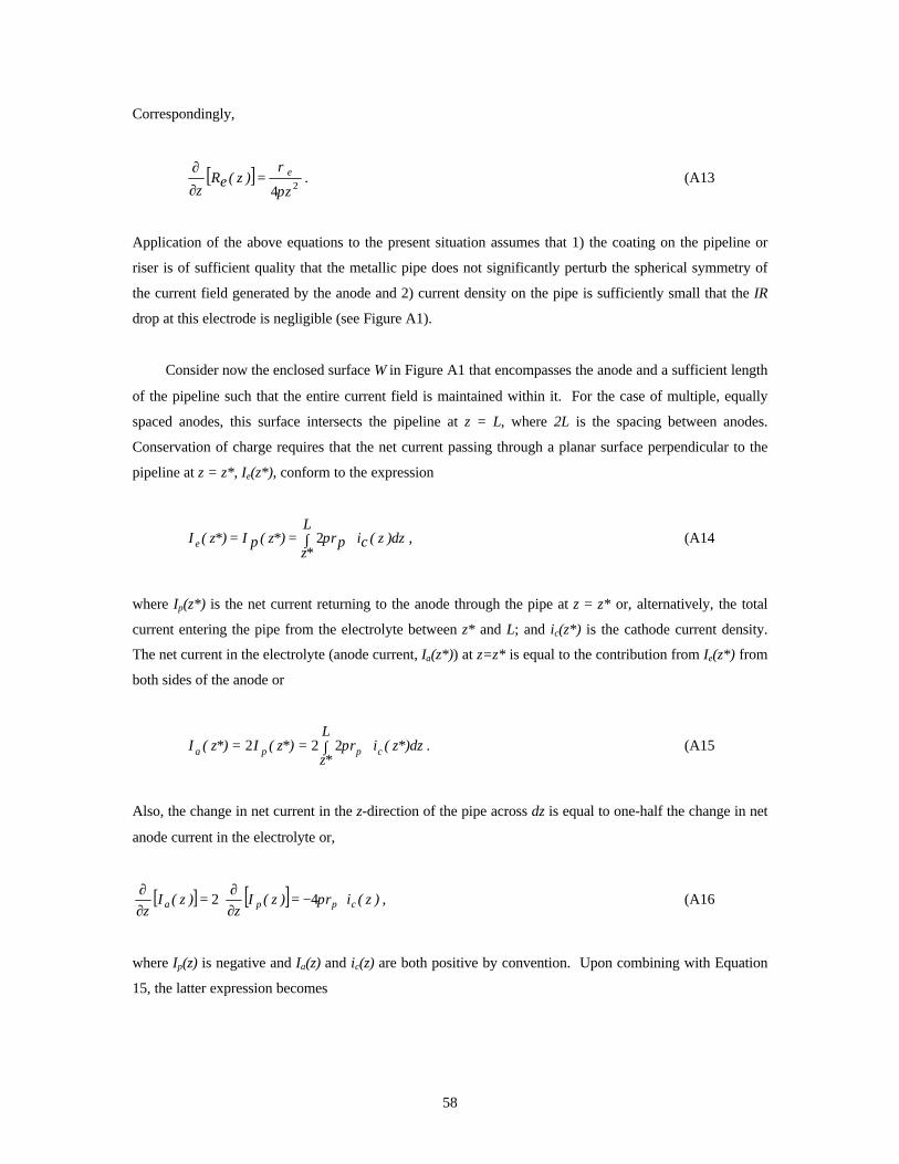
Correspondingly,

r¶ [Re ( z )]= e . (A13¶z 4pz 2

Application of the above equations to the present situation assumes that 1) the coating on the pipeline or

riser is of sufficient quality that the metallic pipe does not significantly perturb the spherical symmetry of

the current field generated by the anode and 2) current density on the pipe is sufficiently small that the IR

drop at this electrode is negligible (see Figure A1).

Consider now the enclosed surface W in Figure A1 that encompasses the anode and a sufficient length

of the pipeline such that the entire current field is maintained within it. For the case of multiple, equally

spaced anodes, this surface intersects the pipeline at z = L, where 2L is the spacing between anodes.

Conservation of charge requires that the net current passing through a planar surface perpendicular to the

pipeline at z = z*, Ie(z*), conform to the expression

L I ( z*) = I p ( z*) = � 2prp � ic ( z )dz , (A14e

z*

where Ip(z*) is the net current returning to the anode through the pipe at z = z* or, alternatively, the total

current entering the pipe from the electrolyte between z* and L; and ic(z*) is the cathode current density.

The net current in the electrolyte (anode current, Ia(z*)) at z=z* is equal to the contribution from Ie(z*) from

both sides of the anode or

L I a ( z*) = 2I p ( z*) = 2 � 2prp � ic ( z*)dz . (A15

z*

Also, the change in net current in the z-direction of the pipe across dz is equal to one-half the change in net

anode current in the electrolyte or,

¶ [I a ( z )] = 2 �¶ [I p ( z )]= -4prp � ic ( z ) , (A16

¶z ¶z

where Ip(z) is negative and Ia(z) and ic(z) are both positive by convention. Upon combining with Equation

15, the latter expression becomes

58

¶ 4prp[I a ( z )] = - � Ec ( z ) . (A17¶z ag

Consider that U ea and U e

c ( z ) are the electrolyte potentials at the anode and pipeline surfaces,

respectively, where the latter is a function of and the former is independent of z, such that the potential

difference between the anode and cathode at z, DU e ( z ) , is given by,

DU e ( z ) = U ea -U e

c ( z ) . (A18

Accordingly, the potential gradient along the pipe may be expressed as,

¶¶ U

ze = -

¶¶ z

[DU e ( z )]= -¶¶ z

[U ea -U e

c ( z )]= -¶¶ z

[-U ec ( z )]. (A19

Then, from Equations A8, 19, A17, and A19,

e¶U

¶z

( z ) =

¶¶ z

[I a ( z )� Re ( z )]= ¶¶ z

[I a ( z )]� Re ( z ) + I a ( z ) � ¶¶ z

[Re ( z )] =

r e � rp Ø 1 1 ø re � rp L

ag � Ec ( z ) � Œ

º ra

-z ϧ

+ ag � �z �z

Ec ( z )dz (A202

and

e c c¶ 2U =

r e � rp � ŒØ��� 1

-1

���œø

� ¶E ( z )

+ 2E ( z )

-2

� �LEc ( z )dz . (A21

¶z 2 ag ŒºŁ ra z łœß dz z 2 z 3 z

Metallic Pipe Potential Variation

¶U The potential gradient in the z-direction within the pipe, m , can be represented in terms of the

¶z

resistance per unit length, Rm, as given by

Rm = r m , (A22Ap

59

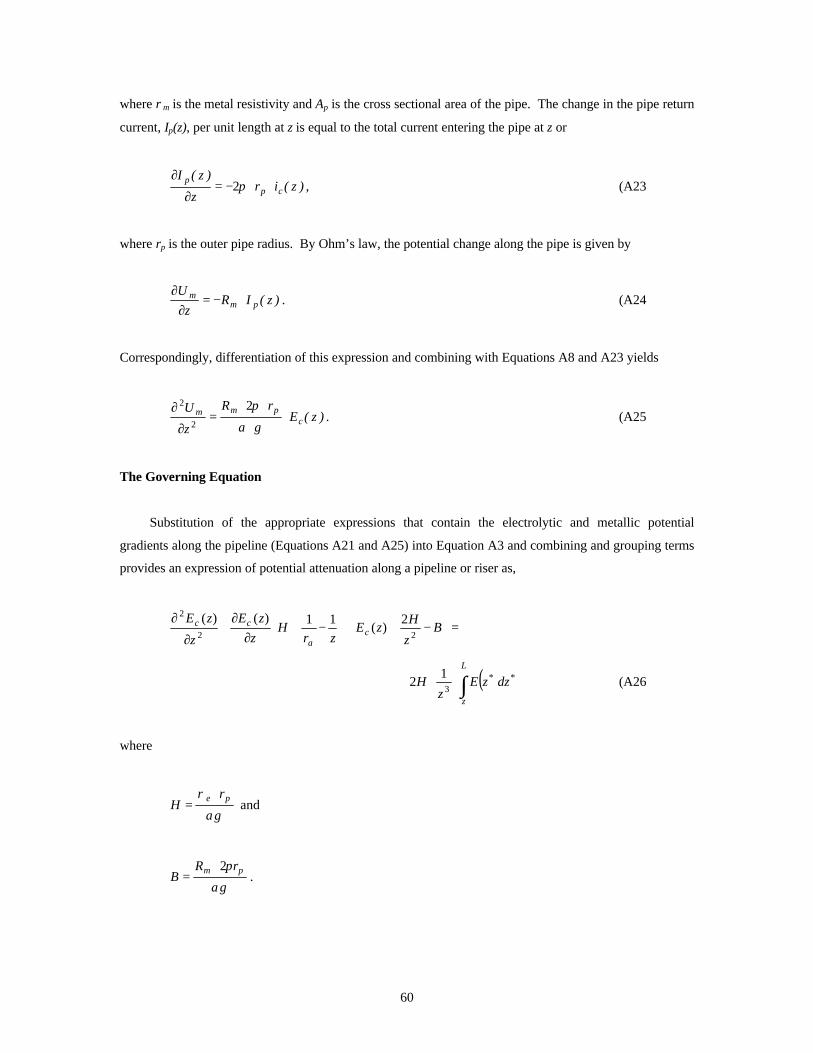
where rm is the metal resistivity and Ap is the cross sectional area of the pipe. The change in the pipe return

current, Ip(z), per unit length at z is equal to the total current entering the pipe at z or

¶I p ( z ) = -2p � rp � ic ( z ) , (A23

¶z

where rp is the outer pipe radius. By Ohm’s law, the potential change along the pipe is given by

m¶U = -Rm � I p ( z ) . (A24

¶z

Correspondingly, differentiation of this expression and combining with Equations A8 and A23 yields

¶ 2U m Rm � 2p �rp

¶z 2 =

a �g � Ec ( z ) . (A25

The Governing Equation

Substitution of the appropriate expressions that contain the electrolytic and metallic potential

gradients along the pipeline (Equations A21 and A25) into Equation A3 and combining and grouping terms

provides an expression of potential attenuation along a pipeline or riser as,

¶ 2 Ec (z) ¶Ec (z) � 1 1 � � 2H �+ � H � �� - �� + Ec (z) � � - B� = ¶z 2 ¶z Ł ra z ł Ł z 2 ł

L

2H � 1

� � E(z* )dz* (A263z

z

where

r � rH = e p

andag

Rm � 2prpB = .

ag

60

APPENDIX B

Spacing Distance between Crossing Pipelines

As part of the present research project, appropriateness of the present MMS regulation that requires a minimum separation distance of 18 inches between crossing marine pipelines has been addressed. In this regard, it is projected that any one of several factors could potentially impact the effect that one pipeline might have upon a second in the vicinity of where they cross. These include, but are not necessarily limited to, 1) miscalculations and uncontrollable occurrences during installation of the crossing pipeline, 2) settlement of one pipeline upon the other with time, and 3) loading of one pipeline by the other in conjunction with a storm or mudslide. From the standpoint of corrosion, the sole question of significance is whether the cathodic protection system of one line might affect the corresponding system and corrosion upon the other. Thus, if the pipelines share a common electrical ground and if one is polarized to a more negative potential (receives greater cathodic protection) than the other, then it can be reasoned that a positive direct current (stray current) could discharge from the former (more negatively polarized pipeline) to the latter (less polarized pipeline). While discharge of positive current from metal into an electrolyte normally results in corrosion (stray current corrosion), such attack should not occur as long as potential for both lines in negative to –0.80 VAg/AgCl. In actuality, such discharge would be from the anode(s) of one pipeline to the other pipeline to an extent that the polarized potential of each approaches the same value. This potentially could cause premature depletion of anodes on the one pipeline. However, such an occurrence should not be affected by separation distance at a point of crossing. In cases where the cathodic protection system on each line is of the galvanic (sacrificial) anode type, as is normally the case, any interactions as alluded to above should not be of significance because of 1) the low driving voltage involved, 2) polarization resistance of the pipeline steel, and 3) the fact that electrical resistivity of steel is about six orders of magnitude less than that of sea water. For this same reason, occurrence of an exceptionally low sea water resistivity, as might occur in conjunction with an eroding salt dome, should be inconsequential. If, however, the cathodic protection system on one or both pipelines is of the impressed current type, then it is possible that negative effects in the form of stray current corrosion could result on one or both of the lines. It is highly unlikely, however, that such corrosion would be influenced by pipeline separation distances that typically exist at a point of crossing (several inches to several feet).