Retirement and House Work: A Regression Discontinuity...

1

Retirement and House Work:

A Regression Discontinuity approach

Elena Stancanelli* and Arthur Van Soest**

October 2011

Abstract

Existing studies show that retirement from the labour market is typically associated with a dramatic

change in the time allocation of individuals. In particular, there is evidence that retirees substitute

home production for private consumption. Earlier studies in this area have considered the behaviour

of the head of the household. In this paper we analyze the causal effect of retirement on the house

work of both partners, allowing for endogeneity of both retirement decisions. Our identification

strategy exploits the fact that for most French workers, the earliest age at which a retirement pension

can be drawn is age 60, which enables us to use a fuzzy regression discontinuity approach to identify

the effect of retirement on time allocation. We find that the retirement probability increases

significantly for partners aged 60 and above, which supports our identification strategy. We conclude

that, not only retirement increases significantly own house work time, but also it affects the partner’s

time allocation. Therefore, controlling for both partners’ retirement is crucial to understanding the

effect of retirement on home production.

Keywords: Time Use, Ageing, Retirement, Regression Discontinuity

JEL classification: D13, J22, J14, C1

*CNRS, University Cergy Pontoise and OFCE, Sciences-Po, Paris

**Netspar, Tilburg University, RAND and IZA

We thank for helpful comments participants at October 2011 Becker’s conference Paris; July 2011 NBER summer institute on Ageing; June 2010 IZA time use conference at Maryland University; April 2010 SOLE conference Vancouver; January 2010 Netspar conference Amsterdam; 2010 CNRS winter school Aussois; and the gender seminar at University Paris 1, Sorbonne Pantheon.

2

1. Introduction

Retirement is one of the key transitions over the life-cycle. It immediately changes the

available time for other activities than paid work and typically increases the time available for

household production, resulting in additional goods and services that may substitute

consumption in the market. In particular, earlier studies argue that the drop in consumption

upon retirement, known as the retirement consumption puzzle, may be at least partly

explained by increased home production. The earlier literature focuses on retirement of the

male head of the household and its effects on consumption and individual home production.

However, retirement of one (or both) of the partners may change the way in which both

partners spend their time. Furthermore, retirement from the labour market of an individual in

a couple may not be independent from retirement of the other partner.

In this paper we analyze the causal effect of retirement (and corresponding changes in paid

work) of men and women in a couple on the time use decisions of both partners, allowing for

endogeneity of both retirement decisions (or both amounts of time spent on paid work). Our

identification strategy exploits the fact that for most French workers, the earliest age at which

a retirement pension can be drawn is age 60. This makes each partner’s probability to be in

retirement a discontinuous function of their age, with a substantial positive jump at age 60.

We therefore can use a regression discontinuity approach to identify the effect of own and

partner’s retirement on the individual allocation of time. In particular, we study the effect of

retirement on the time allocated to home production by partners.

Existing studies show that retirement of an individual is typically associated with a dramatic

change in the time allocation of that individual. For the United States, Mark Aguiar and Erik

Hurst (2005) estimate the effect of retirement (instrumented with age) on individual food

production activities in a remarkable pioneering study in this area. They conclude that retired

people spend more time on home production and thus partly compensate for the fall in their

private expenditure, which explains at least part of the retirement consumption puzzle. In a

companion paper, Aguiar and Hurst (2007) using scanner data and time diaries, find

remarkable evidence that older households spend more time shopping to pay the lowest prices

for identical goods. Consistent with this, Michael Hurd and Susan Rohwedder (2007 and

2008), drawing on records from the Health and Retirement Survey, argue that there is no

retirement consumption puzzle since economic theory can provide explanations for the drop

in consumption around retirement, such as health shocks, changes in the allocation of time or

3

reduction in work-related expenditures. Matthew Brzozowski and Yuqian Lu (2006) find that

in Canadian households, retirement or unemployment leads to substitution of food eaten in

restaurants by food prepared at home and of precooked meals by meals prepared from

primary ingredients, explaining why retirement does not lead to a change in food intake, in

spite of the reduction in food expenditure.

Contrasting evidence is gathered by Erich Battistin, Agar Brugiavini, Enrico Rettore and

Guglielmo Weber (2009) who conclude that private consumption falls significantly at

retirement, though the authors explain most of the drop in consumption by the reduction in

work-related expenditures and children leaving home. In particular, after adjusting their

consumption measure for family size, the effect of retirement on consumption becomes not

significant.

Other studies have focused more generally on the time allocation of older people (see, for

example, Sayer, Liana, Suzanne Bianchi and John Robinson, 2001). Rachel Kratz-Krent and

Jay Stewart (2007), using US data drawn from the American Time Use Survey (ATUS), find

that the time allocation of older individuals varies considerably as a function of their hours of

paid work rather than their age, confirming earlier findings by John Robinson and Geoffrey

Godbey (1997).

The relation between life cycle consumption or home production and retirement has been the

object of a vast literature (see for example, Hamermesh, 1984, or Hurst, 2008) that has

however been conducted disjoint from that on partners’ joint retirement. In the scant literature

on partners' joint retirement decisions one of the explanations for joint retirement is

externalities in leisure: joint retirement makes it possible to derive utility from joint leisure

activities that exceeds the utility from leisure activities without the partner (see, for instance,

Hurd, 1990). Recently, a major contribution in this area is the structural model of retirement

of partners developed by Alan Gustman and Thomas Steinmeier, who estimated their model

with data from the Health and Retirement Study, to conclude that preferences for joint leisure

drive joint retirement choices of partners (2000). Gustman and Steinmeier (2009) push

further their structural model of joint retirement and savings decisions of partners, to

incorporate partial retirement strategies, finding that increased labour force participation of

women has contributed to lower husbands’ hours of market work.

Much less attention is paid to the effect of retirement of one partner in a couple on the time

use of the other partner. Shelly Lundberg, Richard Startz and Steven Stillmann (2003) argue

4

that retirement of the husband lowers the husbands' bargaining power. In particular, the

authors explain the fact that retirement of the primary earner (usually the husband) reduces

household consumption expenditures for couples but not for singles from an increase in the

bargaining weight of the wife, who has a larger preference for future consumption rather than

current consumption, because of longer life expectancy. The authors do not include home

production into the picture.

Here we allow for both the husband and the wife retirement to affect home production. We

specify a recursive model of retirement and time allocation of the two partners, endogenizing

own and partner’s retirement, and identify retirement by using a regression discontinuity

approach. The four equations in this model are estimated jointly by simulated maximum

likelihood. Similarly, we also estimate models in which the dichotomous retirement variables

are replaced by the continuous measures of paid work from the diary data, so that we can

directly analyze how the time that becomes available by reducing or quitting paid work is

reallocated to various home production activities. These include shopping, cooking,

gardening, and, more generally, doing household chores, and caring for adults and children.

All these activities are enjoyable (or better, dislikeable) to different extents and have obvious

market substitutes in the form of maids, gardeners, private enterprises and public or private

care providers. We are not aiming here are at assessing the value of the equivalent market

substitutes (or the corresponding drop in private consumption), but rather to bring the

secondary earner (typically the wife) in to the picture by allowing them to retire as well as to

contribute to home production. This paper focuses on joint retirement and home production

upon retirement of both partners, eliciting various interactions among the two partners. We

are not aware of any earlier study that has investigated this issue.

The data for the analysis are drawn from the 1998-99 French time use survey, carried out by

the National Statistical offices (INSEE). In our data, age is available in months. The sample

includes a thousand of couples where each partner was aged 50 to 70. A time diary was

collected for each partner on the same day, either on a week or a weekend day.

We conclude that the retirement probability increases significantly for spouses aged 60 and

above; and paid work drops significantly, which supports our identification strategy. We find

evidence of strongly significant and positive correlations across the unobservable factors

determining the retirement decisions of the two partners. Our findings indicate that for men in

a couple, it is especially ‘other’ chores, like gardening and house repairs, that increase

5

significantly with retirement, while for women it is ‘core’ house work –including cleaning,

washing up dishes, doing the laundry- and cooking and shopping. To complete the picture,

the time devoted to caring for children or adults from other households increases significantly

for both partners with own retirement.

The structure of this paper is the following. The next section presents the econometric

approach; Section 3 provides details of the data and the sample selection. The exploratory

analysis and the results of the estimations are presented in Sections 4 and 5. The last section

concludes.

2. A regression discontinuity approach

To identify the causal effect of retirement on individual time allocation, we exploit the

legislation on early retirement in France, which sets 60 as the earlier retirement age for

workers in the private sector. This creates a discontinuity in the probability of retirement as a

function of age that enables us to apply a regression discontinuity framework. Excellent

literature reviews of regression discontinuity methods are provided by, for example, David

Lee and Thomas Lemieux, 2010; Wilbert van der Klaauw, 2008; and Guido Imbens and

Thomas Lemieux, 2007. Recent applications of regression discontinuity include, among many

others, Eric Maurin and Aurelie Ouss (2009), Battistin et al. (2009).

Identification of the retirement effect on the time uses is achieved thanks to the sudden and

large increase in the treatment participation at the point of discontinuity (age 60) in the

assignment variable (age). Since individuals cannot manipulate their age, this seems a valid

assumption in our context. In our design the probability of retirement is a function of age

(and other variables) and this function is discontinuous at age sixty. In our data, year and

month of birth were collected, and thus, we assume that age is measured continuously.

However, we need to account for the fact that some people may retire earlier that sixty –due

to special early retirement schemes in the public sector or to specific employment sector rules

- and others later. In particular, the pension benefits payable reach a maximum when

individuals have cumulated a given contribution record (40 years of contributions in the

private sector, at the time of the survey).1 Therefore, individuals that have full pension rights

at the early retirement age have no incentive to retire later. On the contrary, those with lesser

pension benefit entitlement have a disincentive to retire earlier. In particular, this may be the 1 See, for example, Blanchet, Didier and Louis-Paul Pele (1997), and Hairault, Langot and Sopraseuth (2010)

for more details of French pension schemes.

6

case for high educated individuals that delayed entry into the labour market to study longer.

Notice, however, that in France unemployment, maternity and sick leave periods all count

towards the pension contribution period, thus interrupted labour market experience will not

automatically translate into longer work life.

It follows that we are confronted with a “fuzzy” regression discontinuity design and the

probability of retirement at age 60 is greater than zero and less than one. If we did not control

for partner’s (joint) retirement, this would lead to specifying two stages least square

regressions of time use instrumenting retirement with an indicator for being age 60 and above

and interactions of such indicator with (left and right) age polynomials. This is the approach

followed, for example, by David Card, Carlos Dobkin and Nicole Maestas (2004 and 2009);

who studied the effect of individual age eligibility rules to health insurance (Medicaid, to

which anyone is eligible upon reaching age 65 in the United States) ) on individual health

insurance coverage and health related outcomes.

Here we model the effect of retirement of both partners on their time allocation by specifying

a system of simultaneous equations for time uses and retirement of each partner as follows.

Let R be a dummy for retirement, equal to one if individuals have retired from market work

and zero otherwise, and T be the time allocated to a given activity, say house work. The

subscript m stands for male partner and w, for female partner, and we consider time use of

type j:

a) Tjm = Zm βtjm + Zf β

tjf + Rm γtjm + Rf γtjf + Agepolm ψtjm + Agepolf ψ

tjf + νtjm

b) Tjf = Zmλtjm + Zif λ

tjf + Rm δtjm + Rf δtjf + Agepolm ζtjm + Agepolf ζ

tjf + νtjf

c) Rim* = Zm β

rm + Zf βrf + Dm γrm + Agem Dm ηrm + Agem (1-Dm) πrm + Df γ

rf +

+Agef Df ηrf + Agef (1-Df) π

rf + νrm; Rim=1 if Rim*>0 and Rim=0 if Rim

*≤0

d) Rif* = Zm λ

rm + Zf λrf + Dm δrm + Agem Dm τrm + Agem (1-Dm) µrm + Df δ

rf +

+Agef Df τrf + Agef (1-Df) µ

rf + νrf; Rif=1 if Rif*>0 and Rif=0 if Rif

*≤0

Here Agem = [(Agem -60), (Agem -60)2, …. , (Agem -60)n]

Agef = [(Agef -60), (Agef -60)2 ,…., (Agef -60)n]

Agepolm = [(Agem), (Agem)2 , …., (Agem)n]

7

Agepolf = [(Agef), (Agef)2 ,…, (Agef)

n]

The vectors Zm and Zf contain control variables (other than age functions); Dm and Df are

dummies for whether the two individuals have reached age 60; and Age is a polynomial of

order n in age minus 60, which is fully interacted in the retirement equations with the

dummies for being 60 or older; and Agepol is a polynomial of order n in age. The Greek

letters denote vectors of coefficients. The v’s are normally distributed errors, independent of

Zm and Zf and the ages of both partners. The equations for retirement therefore are probit

equations; the time use equations are linear equations. We also experimented with specifying

tobit equations to account for the bunching of some house work activities at zero. In

particular, the zeros may represent infrequent activities rather than activities in which the

individual never participates, which would favour using a linear specification rather than a

tobit-type (see Jay Stewart, 2009, for a thoughtful discussion).

The equations for retirement status of both partners, equations c) and d), explain retirement of

each partner from the control variables of both partners, flexible continuous functions of each

partner’s age, and dummies Dm and Df for whether the two individuals have reached age 60.

The coefficients on the dummies determine the discontinuities at age 60 of the individual and

the partner; we expect the former to be larger than the latter, but if there is joint retirement (in

the sense that the preference for retirement of one spouse increases if the other spouse is

retired), the individual’s retirement decision may also depend on whether the partner is age

eligible for retirement.

The control variables (denoted by Zi) include individual and household characteristics, such

as education level, presence of children, and local labour market variables like the regional

unemployment rate.

The time use equations, a) and b) can be seen as linear demand equations, defining the time

inputs into optimal household production.2 The time use equations include the same control

variables as the retirement equations; a flexible age polynomial and retirement status

dummies of both partners as additional regressors.

2 Taking a more structural approach to model the time allocation of partners, like for example in Laurens

Cherchye, Bram De Rock and Frederic Vermeulen (2010), would not only require additional information on prices and consumption not available in our data, but also imply selecting only couples with positive participation in the time uses considered. See also Vermeulen (2002) for a review of collective models.

8

The four equations will be estimated jointly with simulated maximum likelihood. The error

terms in equations a) – d) are allowed to be correlated in an arbitrary way. This implies that in

this model, own and partner’s retirement are allowed to be endogenous to time use. The

dummies Dm and Df are included in the retirement equations but excluded from the time use

equations: The probability to be retired changes discontinuously when reaching age 60 (and

perhaps also when the spouse reaches age 60), but given retirement status, time use is

assumed to be a continuous function of age. This makes our approach essentially a regression

discontinuity approach.

Alternatively, we also analyze models in which retirement is replaced by paid work time,

obtained from the diary information (for the same day as the other time use variables). This

model uses the same explanatory variables and identification strategy, since reaching age 60

will, through retirement, lead to a discontinuous drop in average hours of paid work (given the

control variables). This enables us to compare more precisely the size of the effects of

reducing hours of paid work on time allocation of men and women in a couple: married

women typically may work shorter hours than married men, affecting the amount of time that

is freed up through retirement, and this may affect the time allocation changes at retirement.

We also use similar models for the total time allocated by the two partners to a given activity,

using a system of three instead of four equations: two retirement equations (one for each

partner) and one time use equation at the household level. The advantage of this is that it

makes it easier to interpret the effect of retirement of one or both partners on the total time

allocated by the couple to say home production. If, for example, retirement of the husband

increases the amount of household chores performed by the husband but equivalently reduces

the amount of chores carried out by his wife, the total home production at the household level

would not be affected.

Finally, because retirement may affect home production during week days but less so on

weekends, we have also estimated the sets of models above (the many variants for retirement,

paid-work, and total house work activity at the couple level) both for week days and the

weekend. This enables us to evaluate the causal effect of retirement on time allocation

performed on different days of the week.

In the framework sketched above, the causal effects we are trying to estimate may have

several sources. First consider the effect of retirement on own time use. Retirement typically

reduces hours of paid work and the time that becomes available must be spent on something

9

else, so that almost automatically retirement will lead to an increase in the time spent on some

activities of the same individual. Second, own retirement as well as retirement of the partner

may directly affect the marginal utility of certain types of time use. Third, retirement may

make it attractive to spend more time on home production, at the same time reducing

expenditures on consumption goods and services bought in the market to compensate for

lower income and usefully exploiting the extra time that becomes available. This is one of the

potential explanations for the retirement consumption puzzle, the phenomenon that

consumption expenditures tend to fall at retirement. Fourth, retirement of either partner may

change each partner’s bargaining power within the household, which may change the

outcomes of the household decision process. Changes in bargaining power may also affect the

share of home production that is produced by each partner (see Robert Pollak 2005 and 2010),

as well as the optimal amount of total home work to be done within the household (if the

partner with the larger bargaining power has stronger preferences for home production, the

couple may produce relatively more of the home produced good than under the opposite

scenario).

If the retirement decision is exogenous to the time allocation choices, it would not be

necessary to rely on regression discontinuity for identification. To test the sensitivity of our

results to allowing for endogenous retirement, we also estimate the same time allocation

equations separately (that is, not jointly with retirement equations), taking retirement as an

exogenous variable, and compare the estimated effects of retirement on time use under the

two specifications.

3. The data: sample selection and covariates


the National Statistical offices (INSEE). This survey is a representative sample of more than

8,000 French households with over 20,000 individuals of all ages –from 0 to 103 years. Three

questionnaires were collected: a household questionnaire, an individual questionnaire and the

time diary. The diary was collected for all individuals in the household, which is an

advantage over many other surveys that only have information on one individual in each

household. The diary was filled in for one day, which was chosen by the interviewer and

could be either a week day or a weekend day. This was the same day for all household

members.

10

3.1 Sample selection

Selected couples, married or unmarried but living together, gave a sample of 5,287 couples

with and without children. We then applied the following criteria to select estimation samples

of older men and women in a couple.

• Each respondent was aged 50 to 70.

• Each respondent had filled in the time diary.

• No respondent had filled in the time diary on an “exceptional day”, defined as a

special occasion such as a vacation day, a day of a wedding or another party, etc.

• The respondents were not unemployed.

• We dropped one man who reported to be a home-maker, but we kept housewives.

Applying these criteria led to a sample of 1043 couples.

3.2 Diary activities and covariates

The diary was filled in by each household member on one specific day, either a week day or a

weekend day, according to the following procedures:

a) The interviewer chose the day the diary should be filled in.

b) The diary covered a 24 hours time span, with activities recorded every ten minutes.

c) Main and secondary activities were coded, where the latter were defined as activities

carried out simultaneously with another, primary, activity (for example, cooking and

watching the children). The respondent decided which activity should be coded as

primary and which as secondary (if any).

d) About 140 categories of main activities and 100 categories for secondary activities

were distinguished in the design of the survey.

Here we only consider activities reported as main activity. Very few respondents filled in

secondary activities. We distinguish the following activities:

1. Paid work, whether at home or at the office.

2. House work, and its subcomponents:

2.1.‘Core’ household work, including time spent cleaning, doing the laundry, ironing,

cleaning the dishes, setting the table, and doing administrative paper work for the

household.

11

2.2.Shopping

2.3.Cooking

2.4 “Other” household work, including time devoted to gardening, house repairs, knitting,

sewing, making jam, and taking care of pets.

3. Caring for children and/or adults living in the same or in other households

We separate cooking and shopping activities from other ‘core’ chores as these two activities

are the ones that received most attention in the earlier American literature on substituting

home production for private expenditure (Aguiar and Hurst, 2005 and 2008). We also single

out ‘other’ house work, sometime denominated as “semi-leisure’ chores in the time use

literature, the assumption being perhaps that doing the garden or house repairs are tasks

somewhat more enjoyable than other sorts of house work. Indeed, the limited information

available to date on individual preferences suggests that most people dislike “core” chores

like cleaning, doing the dishes, the washing, and ironing, but a larger fraction enjoys cooking

or shopping; and an even larger proportion enjoys doing house repairs (see Elena Stancanelli

and Leslie Stratton, 2010, for some evidence). One could potentially hire a maid, a gardener

or an enterprise to perform most of these activities. Finally, earlier studies show that one

should be careful about aggregating care tasks and household chores (for example, Rachel

Connelly and Jean Kimmel, 2009), listed under categories two and three above. In particular,

the care activity includes here diary reported activities like bathing the children, feeding them,

helping them with homework, playing with them, taking them somewhere, giving medical

treatment to adults, and taking care of them. Care activities generally have obvious labour

market substitutes, either institutional or marketwise like private care providers.

In our data, age is available in months. The employment or retirement status is derived from

the respondent’s self-assessed occupational status. The indicator for retirement takes value

one for respondents that reported to be retirees or early-retirees.

We constructed an indicator for time diaries filled in on a weekend day. In the models using

paid work instead of retirement and looking at house work on different week days, this

indicator was interacted with the paid work amount in the time allocation equations; and with

the age dummies for having reached age 60 in the paid work equations.

As far as the other covariates go, the number of children in the household includes dependent

children up to 18 years of age. Three education levels are distinguished: low (less than twelve

12

years of schooling), intermediate (twelve years of schooling), and high (over twelve years of

schooling). The unemployment rate is the regional unemployment rate at the time of the

survey. Paris is an indicator for whether individuals reside in the city of Paris. Cohabiting

individuals are those living together but not formally married. Bad health is an indicator

which is equal to one if individuals report to have bad or very bad health status -health is self-

assessed on a scale from 1 to 5: very good, good, medium, bad, or very bad.

3.3 Descriptive statistics

Descriptive statistics for the samples are given in Table1. We have selected a sample with

both partners aged between 50 and 70 years (see Section 3.1). Women are on average two

years younger than their husbands. About 57 per cent of the men and 43 of the women in a

couple, in our sample, are aged 60 or above. And, somewhat consequently, 64 per cent of the

men and 33 per cent of the women in the sample report to have retired from market work.

Remember that our sample also includes housewives, as in order to have a balanced sample

we have kept these couples in (see Section 3.1 for more details). The percentage employed is

about the same for both partners; only slightly larger for men that are employed 36 per cent of

the time against 32 per cent for women. Only a small minority of individuals were not born in

France: 4 per cent of the men and 3 per cent of the women. The majority of individuals have

less than twelve years of schooling (the benchmark). Men tend to be slightly more educated

than women: 12 (10) per cent of husbands (wives) have completed intermediary education (12

years of schooling) and 15 (11) per cent have a higher education level (over twelve years of

schooling). Only 15 per cent of the sample has children still living the parental home. Only

4 per cent of the couples are cohabiting; the others are formally married. Very few couples (2

per cent) were living in central Paris. The mean level of unemployment at the time was

pretty high, over eleven per cent.

These findings are due to a combination of having selected older generations and only those

in a couple, as younger generations in France tend to be more educated and more often

cohabiting. Only three per cent of the men and five per cent of the women in our sample

reported to have a bad general health status. This percentage is probably lower than in the

complete population since disabled workers were dropped from the sample.

About 23 per cent of the observations filled in the time diary on a weekend.

13

Descriptive statistics of participation, mean and median diary day duration, in minutes, for

various time uses (see Section 3.2 for more details of the definition of the diary activities

considered here) are provided in Table 2. Harley Frazis and Jay Stewart (2011) provide a

very thoughtful account of how to carefully interpret distributional information drawn from

diary data.

In line with below average employment rates, only 30 per cent of the men and 22 per cent of

the women report any paid work activity on the day the diary was collected, knowing that 23

per cent of these days fell on a weekend. Average paid work including the zeros is slightly

over two hours a day for men and slightly less than an hour and a half for women. The

median of hours of paid work is zero for both partners. Using a standard definition of

housework, that includes all chores (as listed at point 2 of the data section above), 87 per cent

of the husbands and 99 per cent of the wives report doing some house work on the diary day.

On average, husbands spends three hours on it and wives five hours, on a given day –which

might be a weekend day. Excluding ‘other’ chores, the amount of ‘core’ housework (which

includes cleaning, cooking, shopping, washing clothes, ironing, doing the dishes, and doing

administrative paper work) done by husbands falls dramatically, to one hour and a quarter, on

average, while for women the difference is only half an hour less. The median man spends

indeed an hour on ‘other’ chores (gardening, house repairs, etc, see list above in the data

section) against no time at all for the median woman in our couple sample. Participation in

these tasks is almost 62 per cent for husbands against 44 per cent for wives. To give some

order of reference, the participation rate in cooking is 93 per cent for women and 30 per cent

for men while 41 per cent of the men and 52 per cent of the women do some shopping on the

diary day.

Next, we provide some information on care activities by the couples in our sample. This

variable includes care provided to children and adults living at home or belonging to other

households and it includes performing house work for adults in other household for no charge

(see Section 3.2 for more details). The participation rates of men is 15 per cent and that of

women 22 per cent; and the average time allocated to it on the diary day is 18 minutes for the

first, and 24 for the second.

Of course, all these comparisons relate to our sample of older couples; the picture may be

quite different for singles or younger people.

14

Exploratory graphical analysis

It is now time to carry out some exploratory graphical analysis of the discontinuities in,

respectively, retirement or paid work, and time allocation upon reaching age 60 and above for

each partner. In line with the regression discontinuity literature (see Lee and Lemieux, 2010;

Wilbert van der Klaauw, 2008; and Imbens and Lemieux, 2007, for an account), to detect

graphically the expected jump at the point of discontinuity (age 60 here or, more precisely,

720 months since month and year of birth) in the assignment variable (age), we split the

sample into equally sized bins. We use here bins of size tens.3

Individual retirement status (and, alternatively, the time devoted to paid work) is plotted

against age to inspect jumps in the retirement probability at age 60 (720 months) and above in

Charts 1.4 Notice that for simplicity, here housewives are considered as retired women, as

opposed to those employed and thus, still at work. This adds to the motivation for also

looking at the drop in paid work. Paid work is measured here using diary reports on the

amount of paid market work performed on the diary day. There is an obvious discontinuity at

the age cutoff of 60 for both men and women in our couple sample.

Total housework (see Sections 3.2 for details) and total care time are plotted against age in

Chart 2. There is a sharp increase in housework carried out by men around age 60 (720

months here). The pattern is less clear for care work.

‘Core’ housework and ‘semi-leisure’ house chores (two subcomponents of housework) are

plotted against age in Chart 3. The increase in ‘semi-leisure’ chores of men at age 60 (720

months of age) is quite sharp, while the same cannot be said for women’s ‘semi-leisure’

chores that actually drop at age 60, as perhaps their retired husband takes them over. As far

as ‘core’ housework is concerned, the pattern is less straightforward.

Chart 4 plots the time allocated to cooking or shopping against age. There is an increase at

age 60 in these time uses for men, but less so for women.

To sum up, for some of unpaid work activities considered, the plots suggest that there is a

substantial jump at age 60. In our regression discontinuity framework, these discontinuities

are due to the discontinuity of the retirement probability at age 60 in Chart 1 (or the drop in

3 Using smaller or larger bins does not affect the jump at age 60 for either men or women in a couple.

15

paid work) combined with a substantial effect of retirement (or the drop in paid work) on the

time spent on the activity. The identifying assumption is that there is no discontinuous jump

of the direct effect of age on each type of time use. Essentially this is also the identification

strategy of the econometric models discussed in the previous section and estimated below,

where we allow for more flexible continuous age patterns to the left and right of age 60, and

where we control for a number of individual characteristics other than age or occupational

status.

4. Estimation results

We have estimated simultaneous model of retirement (paid work) and time uses of partners by

simulated maximum likelihood, using 100 draws. 5 The explanatory variables of the

retirement equations include dummies for age 60 (that is to say, 720 months of age) and older,

and left and right cubic polynomials in months of age of the two partners interacted with the

age 60 (720 months of age) dummies (see Section 2). 6 The coefficients on the dummies

determine the discontinuities at age 60 of the individual and the partner. The other regressors

included in the retirement (paid work) equations are: an indicator for whether the couple

resides in Paris; a cohabiting dummy; the regional unemployment rate; the number of

children; and indicators for whether each partner holds an intermediate or higher degree. The

time use equations include the same control variables and a flexible cubic polynomial in age,

and add the retirement status dummies of both partners as additional regressors.7 The error

terms of the equations of the system are assumed to be jointly normally distributed and we

also estimate their unrestricted correlations.

First of all, we present results of estimation of the model of the effect of retirement (paid

work) on house work, defined as broadest as possible, to include ‘core’ house work -cleaning,

ironing, doing the laundry, doing the dishes, setting the table, cooking, shopping- and ‘other’

chores -gardening, doing house repairs, taking out dogs, doing jams, or knitting. Results of

estimation are provided in Table 3, marginal effects in Table 4. Results of estimation of a

similar model for paid work are given in Table 5. We show all the estimates except for the

5 See Roodman, 2007 and 2009, for details of the procedure that we used.

6 In the models that distinguish week days from weekends, we also include cross-effects of age 60 (720 months

of age) dummies and weekend diary in the paid work equations. 7 We also control for a weekend dummy and its interactions with the retirement (paid work) dummies, in the

models that distinguish week days from weekends.

16

many coefficients on the age polynomials and their interactions with the age 60 dummies (that

are shown, separately, in Table 5B) 8 and the estimates of the correlation terms (shown in

Tables 3a and 5a, respectively).

We conclude that the retirement probability increases (paid work falls) significantly for

individuals in a couple aged sixty and over. Marginal estimates for the retirement equations

(see Table 4) are calculated at the mean value of the continuous explanatory variables and, for

dichotomous ones, assuming lower than intermediate education for both partners, no

residence in Paris, formal marital status (setting cohabiting to zero) and that both partners are

aged 60 years or more. This leads to the conclusion that the retirement probability increases

by 0.23 (0.13) percentage points for married men (women) aged 60 and above. The fact that

partner reaches age sixty has no significant effect on individual retirement (paid work). We

find that own retirement increases significantly husband’s wife’s house work time (see Table

3). For both partners the effect is much stronger during week days than on weekends, when

house work does actually fall upon retirement. The overall average effect of retirement on

house work is positive for both partners but less sizable once the negative drop on weekends

is taken into account. Retirement of the wife reduces considerably the amount of house work

carried out by men during week days while their weekend housework is not affected.

Husband’s retirement has no significant effect on the amount of house work carried out by

women.

As far as the other covariates go, individuals living in inner Paris and the higher educated

retire later than the others. Women married to a higher educated men retire slightly earlier

than the others (the coefficient on his high education level is positive tough significant only at

the ten per cent level).

Results for paid work are more or less the “mirror” image of this (see Table 5). Own paid

work falls dramatically and significantly upon reaching age 60 for both partners, with this

effect being larger for men. The drop in paid work at age 60 and older is much larger on

week days than on weekends, as reasonable. At weekends paid work falls significantly for

both partners and the drop is larger than that found for individuals aged 60 and above,

8 Most of them are not significant, except for the coefficients on the interaction with the squared and cubic term from the left polynomial for husbands that are strongly significant and negative. Similarly, the equivalent terms for the wife in the paid work model (the mirror picture of retirement) are strongly positive. They may suggest some postponing of retirement.

17

suggesting that few people worked on a weekend day, in France in 1998. Whether the partner

is 60 or older has no significant impact on own paid work.

Paid work reduces dramatically the time devoted to household chores by partners, though this

effect is significant only at the ten per cent level for women. His house work increases

significantly in response to the wife paid work on weekends.

The unobservable factors affecting his and her retirement (paid work) are positively and

strongly correlated; and so are the errors of his and her house work (see Table 3a and 5a).

Next, we re-estimate our model removing the assumption that the retirement status may be

endogenous to the time allocation decision. Results are shown in Table 6, respectively, for

retirement (columns two and three) and paid work (columns four and five). Remarkably, the

estimated effect of retirement on house work is almost unaffected. The coefficients are very

close to those estimated in Table 3, especially for those effects that showed up significant.

Differences are also small though more sizeable for the paid work model. These findings

would suggest that individuals do not retire earlier to spend more time on house work. Of

course, this could be different for some of the other activities that we consider that may be

more enjoyable. Thus we opt for continuing to instrument retirement as in our preferred

specification.

Then, we provide in Tables 7 to 12, a selected set of estimates of the effect of retirement on

unpaid house work –total housework and its subcomponents, ‘core’ house work, cooking,

shopping, ‘other’ chores and care time. For each time activity, we estimate two sets of

models. In the first, the left hand side variables include each partner’s time, leading to four

simultaneous equations: two for retirement of each partner and two for the time use of each

partner. Under the other specification, the relevant left hand side variable for the time use, is

the total time devoted by the partners to the activity, obtained summing up the time allocated

by each and this gives a system of three simultaneous equations: two for retirement of each

partner and one for the total time devoted to the activity. Similar models are estimated for

paid-work (instead of retirement) and the relevant selected estimates are reported in Tables 13

to 18, which helps us quantify the effects. In the same set of tables (at the risk of some

confusion, but gaining considerably on conciseness), we also show the effects for week days

and weekends, which indicate that generally most of the effect of retirement on home

production occurs during week days, as partners reallocate time from paid work to home

production, while their weekend time allocation is not significantly affected by retirement. It

18

is worth mentioning that the various estimates shown in each activity table are obtained from

estimating different models and this is why the coefficients do not simply add up. For

example, if retirement increases women’s shopping time but not men’s, and if most of the

shopping is typically done by the husband, the overall increase in household shopping at

retirement may turn out not be statistically significant. When comparing week or weekend

day estimates to the overall effects, bear in mind that a weekend day only occurs twice a

week.

For the sake of clarity, we only show the coefficients of interest.

Table 7 indicates that the total housework produced by the household increases by over four

hours on a representative day, following the retirement of the husband from the labour

market; while the retirement status of the wife does not have a significant effect overall,

because it affects negatively the housework done by the husband and positively that carried

out by the wife –and these two effects are very close in absolute value. We can also see that

all of the increase in housework occurs on weekdays while nothing changes for the weekend.

In particular, for every minute drop in paid-work, his housework increases by half a minute

(see Table 13).

However, looking at core housework (Table 8), defined as more “compulsory” tasks such as

cleaning, ironing, doing the laundry and the dishes, our results suggest that it is her retirement

that increases the time devoted to these activities, while his retirement has no overall effect,

except for reducing the amount done by him on weekends. Interestingly, her retirement

increases both his and her time spent on core housework. His core housework increases on

week days and also on weekends, following her retirement. In particular, the increase in his

weekend core housework upon her retirement is much larger (almost twice as much) than the

drop registered following his retirement. However, these effects are not significant in terms

of the responses to the drop in partners’ paid work (see Table 14), which is perhaps due to the

fact that many of the women in the sample are housewives anyhow and thus only a small

proportion of women do actually retire from the labour market.

Similar effects for other chores, that include gardening, doing house repairs, taking care of

pets, doing jams, knitting and sewing, are reported in Table 9 for the retirement models and in

Table 15, for paid-work. We find that much of the increase in total housework (see Table 7

and the related discussion above) can be ascribed to the additional time that husbands allocate

to these activities. In particular, men in a couple devote more than three extra hours to these

19

chores upon their retirement, though less so if their wife is also retired (by almost two hours

less in this case). Men’s ‘semi-leisure’ chores increase substantially both on weekdays and

weekends upon their retirement, and significantly less so on either week or weekend days if

their wife retires. In contrast, her ‘semi-leisure’ chores are totally unaffected by his or her

retirement (there is a small increase for her weekdays following her retirement but only

significant at the ten per cent level; and this effect is wiped out by the large negative effect her

retirement has on his chores here). To sum up, every minute drop in paid work by men results

in 15 seconds increase in ‘semi-leisure’ chores at the household level (see Table 15). Some

further analysis (not shown) indicates that it is mostly house repairs and gardening that drive

these results (roughly half of the individuals in the sample have access to a garden); the

change in the amount of time devoted to pet care being small and that allocated to the other

activities listed irrelevant.

Remarkably, the time devoted to cooking (see Table 10) and shopping (see Table 11) at the

household level increases significantly, by over one hour, for cooking, and by almost 50

minutes for shopping, on a given day, with her retirement from the labour market. The effect

of his retirement is overall statistically not significant (estimates shown on the right-hand top

box of Tables 10 and 11). In particular, the time he devotes to shopping any week or weekend

day falls significantly with his retirement and increases significantly with hers. In contrast, her

shopping time is almost unaffected by her or his retirement, except for her shopping time on

weekdays which increases upon her retirement, but the coefficient is only significant at the ten

per cent level. We find comparable overall effects for cooking. However, here her retirement

increases significantly the time she spends cooking both on week and weekend days but has

no significant impact whatsoever on his cooking (the estimated effect of her retirement on his

cooking is small and positive, significant at ten per cent only for weekends) ; while his

retirement reduces his cooking time on week or weekend days but does not affect her

cooking. Like for core housework, we find no evidence of a significant relation between the

drop in paid-work at age 60 and above and the time allocated to shopping (Table 16) or

cooking (Table 17) by either partner. Although her paid work increases significantly his

cooking time, the size of the impact is very tiny. In particular, her paid work, especially on

weekdays, reduces significantly her cooking and increases significantly his, but these effects

are very small. The time he devotes to cooking or shopping falls significantly on week days

with his paid-work but the size of the impact is tiny. This may possibly be due to the fact that

women tend to work fewer hours than men and thus, changes, in house work of women due to

20

the drop in their paid work upon retirement are not very sizeable. To reconcile this with our

earlier findings, we find significant increases in shopping, cooking and other ‘core’ chores

(cleaning, doing the washing and the dishes) carried out by women upon retirement but the

size of this effect is very small.

Finally, Tables 12 and 18, report selected estimates of the changes in partners’ caring time

due to, respectively, their retirement or the reduction in their paid-work minutes. We conclude

that own retirement increases significantly the time each ones allocates to caring for others,

and especially so for men, whose caring time increases by 15 seconds for each minute drop in

paid-work .

To sum up, our findings indicate that for French men in 1998, it is especially semi-leisure

chores that increase significantly with retirement, while for women it is core house work,

cooking and shopping. In particular, he spend significantly more time on core chores and

shopping if his wife retires while the opposite holds true for his semi-leisure chores that drop

dramatically if she retires. Looking at the sum of all these house work components at the

household level, we conclude that total housework increases significantly with his retirement

but is not responsive to hers. This last finding is mainly due to the negative effect of her

retirement on his semi-leisure chores and it suggests that considering only the aggregated

house work effects at the household level is misleading.

To complete the picture, the time devoted to caring for others increases significantly for both

partners with own retirement.

To conclude, we have gathered evidence that controlling for both partners retirement is

crucial to understanding the effect of retirement on home production.

As robustness checks go, using tobits type specifications instead of linear equations for house

work, did not affect substantially our conclusions.

6. Conclusions

The time allocation of individuals changes dramatically at the time of retirement. There is a

scant literature suggesting that retirees substitute home production for private expenditure.

However, earlier literature did not take the secondary earner, typically the wife, into account,

at least to our knowledge. Because women tend to perform disproportionate amounts of home

21

production and recent studies find that partners tend to retire together, it is our aim to allow

here for both partners’ retirement and house work activities.

For most French workers, the earliest age at which a retirement pension can be drawn is age

60, which enables us to use a regression discontinuity approach to study the effect of

retirement on home production activities of older French partners. These include shopping,

cooking, gardening, and, more generally, doing household chores, and caring for adults and

children. Although these activities have obvious market substitutes, we are not aiming here at

assessing the value of the equivalent market substitutes (or the corresponding drop in private

consumption), but rather to bring the secondary earner (typically the wife) in to the picture by

allowing them to retire as well as to contribute to home production. Thus, this paper

investigates joint retirement and home production upon retirement of both partners, eliciting

various interactions among the two partners, within a regression discontinuity type of

framework. We specify a recursive model of retirement and time allocation of the two

partners, endogenizing own and partner’s retirement. The equations in this model are

estimated jointly by simulated maximum likelihood. Similarly, we also estimate models in

which the dichotomous retirement variables are replaced by the continuous measures of paid

work from the diary data, so that we can directly analyze how the time that becomes available

by reducing or quitting paid work is reallocated to various activities.


the National Statistical offices (INSEE). In our data, age is available in months. The sample

includes a thousand of couples where each partner was aged 50 to 70. A time diary was

collected for each partner on the same day, either on a week or a weekend day.

We find that the retirement probability increases significantly for spouses aged 60 and above;

and paid work drops significantly, which supports our identification strategy.

To sum up, our findings indicate that for men in a couple, it is especially chores like

gardening and house repairs that increase significantly with retirement, while for women it is

core house work, like cleaning, shopping and cooking. In particular, married men spend

significantly more time on core chores if their wife retires while the opposite holds true for

gardening and repairs that drop dramatically if she retires. Looking at the sum of all these

house work components at the household level, we conclude that this increases significantly

with his retirement but is not responsive to hers. This finding is mainly due to the negative

22

effect of her retirement on some of his chores and it suggests that considering only the

aggregated house work effects at the household level is misleading.

To complete the picture, the time devoted to caring for others increases significantly for both

partners with own retirement.

In conclusion, we have gathered evidence that controlling for both partners retirement is

crucial to understanding the effect of retirement on home production.

References Aguiar, Mark and Eric Hurst (2007) "Life-Cycle Prices and Production," American Economic Review, American Economic Association, vol. 97(5), pages 1533-1559, December Aguiar, Mark and Eric Hurst (2005), "Consumption versus Expenditure", Journal of Political Economy, 113, no.5, 919-948. Battistin, Erich, Agar Brugiavini, Enrico Rettore and Guglielmo Weber (2009), "The Retirement Consumption Puzzle: Evidence from a Regression Discontinuity Approach American Economic Review, 99(5), 2209-2226. Blanchet, Didier and Louis-Paul Pele (1997), Social Security and Retirement in France, NBER Working Paper No. 6214. Brzozowski, Matthew and Yuqian Lu (2006), Home cooking, food consumption and food production among the unemployed and retired households, SEDAP Research Paper No. 151, McMaster University, Hamilton, Ontario, Canada. Card, David, Carlos Dobkin and Nicole Maestas (2009), "Does Medicare Save Lives? ", Quarterly Journal of Economics, 124(2), 597-636. Card, David, Carlos Dobkin and Nicole Maestas (2004), "The Impact of Nearly Universal Insurance Coverage on Health Care Utilization and Health: Evidence from Medicare", NBER Working Paper 10365, March. Harley Frazis and Jay Stewart (2011), “How to Think About Time-Use Data: What Inferences Can We Make About Long- and Short-Run Time Use from Time Diaries?”, Annals of Economics and Statistics, forthcoming. Laurens Cherchye, Bram De Rock and Frederic Vermeulen (2010), “Married with Children: A Collective Labor Supply Model with Detailed Time Use and Intrahousehold Expenditure Information”, IZA DP, September. Connelly, Rachel and Jean Kimmel (2009), "Spousal Influences on Parents' Non-market Time Choices," Review of the Economics of the Household, 7(4), 361-394.

23

Gustman, Alan and Thomas Steinmeier (2009), “Integrating Retirement Models,” NBER Working Paper 15607, December. Gustman, Alan and Thomas Steinmeier (2000), “Retirement in Dual-Career Families: A Structural Model,” Journal of Labor Economics, 18, 503-545. Hairault, Jean-Olivier , Francois Langot and Thepthida Sopraseuth (2010), "Distance to Retirement and Older Workers' Employment: The Case for Delaying the Retirement Age," Journal of the European Economic Association, vol. 8(5), pages 1034-1076, 09. Hamermesh, Daniel S. (1984), "Consumption During Retirement: The Missing Link in the Life-Cycle," Review of Economics and Statistics, vol. 66(1), pages 1-7. Hurd, Michael (1990), "The Joint Retirement Decision of Husbands and Wives," in: Issues in the Economics of Aging, David Wise (ed.), National Bureau of Economic Research, pp. 231-258. Hurd, Michael, and Susann Rohwedder (2007), "Time-Use in the Older Population: Variation by Socio-economic Status and Health," RAND Working Papers 463. Hurd, Michael, and Susann Rohwedder (2008), “The Retirement Consumption Puzzle: Actual Spending Change in Panel Data”, NBER WP No. 13929, April 2008. Hurst, Erik, (2008): “The Retirement of a Consumption Puzzle,” NBER Working Papers 13789, National Bureau of Economic Research, Inc. Imbens, Guido and Thomas Lemieux (2007), "Regression discontinuity design: a guide to practice", Journal of Econometrics, 142, 615-635. van der Klaauw, Wilbert (2008), "Regression-Discontinuity Analysis: A Survey of Recent Developments in Economics, Labour, 22(2), 219-245. van der Klaauw, Wilbert (2002), "Estimating the Effect of Financial Aid Offers on College Enrollment: A Regression-Discontinuity Approach”, International Economic Review, 43(4), 1249-1287. Krantz-Kent, Rachel and Jay Stewart (2007), " How do older Americans spend their time?", Monthly Labor Review, May, 8-24. Lee, David, S. and Thomas Lemieux (2010), "Regression Discontinuity Designs in Economics", Journal of Economic Literature, 48(2), 281-355. Lundberg, Shelly, Richard Startz, and Steven Stillman (2003), "The Retirement-Consumption Puzzle: A Marital Bargaining Approach", Journal of Public Economics, 87(5-6), 1199-1218. Maurin, Eric and Aurelie Ouss (2009), "Sentence Reductions and Recidivism: Lessons from the Bastille Day Quasi Experiment," IZA Discussion Papers 3990. Pollak, Robert A. (2005), “Bargaining Power in Marriage: Earnings, Wage Rates and Household Production.” NBER Working Paper No. 11239 (March).

24

Pollak, Robert A. (2010), “Individuals' Technologies and Household Technology.” Washington University in St. Louis, mimeo. Robinson, John and Geoffrey Godbey (1997), "Time for Life: The Surprising Way Americans Spend Their Time", University Park, The Pennsylvania State University Press. Roodman, David (2009), “Estimating Fully Observed Recursive Mixed-Process Models with cmp.” Working Papers 168, Center for Global Development. Roodman, David (2007), “CMP: Stata module to implement conditional (recursive) mixed process estimator.” Statistical Software Components S456882, Boston College Department of Economics, revised 22 May 2009. Sayer, Liana, Suzanne Bianchi and John Robinson (2001), "Time Use Patterns of Older Americans," Report to NIA, University of Maryland. Stancanelli, Elena and Leslie Stratton (2010). "Her Time, His Time, or the Maid's Time: An Analysis of the Demand for Domestic Work", IZA DP 5253.

Stewart, Jay. (2009). ``Tobit or Not Tobit?'' IZA Discussion Paper 4588.

Szinovacz, Maximiliane (2000), "Changes in Housework After Retirement: A Panel Analysis", Journal of Marriage and Family, 62 (1), 78–92. Vermeulen, F. (2002), "Collective household models: principles and main results", Journal of Economic Surveys, 16, 533-564.

25

Table 1. Sample descriptives

Male partner Female partner

Mean standard deviation Mean standard deviation

Age 60.72 5.50 58.60 5.61 Age 60 or older 0.57 0.49 0.43 0.47 Retired 0.64 0.48 0.33 0.47 Employed 0.36 0.48 0.32 0.47 Born in France 0.96 0.18 0.97 0.16 Intermediate ed. (12 years schooling)

0.12 0.32 0.10 0.30

Higher education ( over 12 years of schooling)

0.15 0.36 0.11 0.31

Children at home no.

0.15 0.51

Cohabiting 0.04 0.19 Resides Paris 0.02 0.15 Regional U 11.45 2.46 Bad health 0.03 0.18 0.05 0.23 Weekend diary 0.23 0.42 Observations 1043

Note: Age is measured in years and fractions of years (months); diary activities in minutes.

26

Table 2. Participation rate and mean duration of diary day activities

Male partner Female partner

Participation rate %

Mean duration (st. dev.)

Median duration

Participation rate %

Mean duration (st. dev.)

Median duration

Paid work 29.82 137.83 (235.46)

0 21.67 86.04 (182.88)

0

House work 86.77 183.70 (152.56)

160 99.04 310.60 (147.40)

310

House work , excluding semi-leisure

70.18 77.19 (88.64)

40 98.85 264.85 (123.81)

260

Core Housework (excludes a, b, and c)

50.81 36.38 (59.05)

10 96.07 145.04 (90.28)

140

Cooking, a 29.63 11.40 (24.09)

0 93.38 81.67 (49.15)

80

Shopping, b 40.84 29.42 (47.97)

0 52.06 38.14 (49.96)

10

Semi-leisure, chores, c

61.74 106.51 (128.64)

60 43.72 45.75 (75.36)

0

Caring for children and/or adults

14.67 17.66 (66.12)

0 21.76 24.31 (65.13)

0

Observations 1043

Note: activities are measures in minutes. The sample includes week and weekend diaries. The diary was collected the same day for both partners, which was chosen by the interviewer. Weekend diaries are 23 per cent of the diaries.

27

Chart 1. Retirement and Paid Work: discontinuities at age 60

28

Chart 2. House work and care time: discontinuities at age 60

7111

616

120

525

0M

ean

of h

ouse

wor

k, h

usba

nds

50 55 60 65 70age

263

286

309

332

355

Mea

n of

hou

se w

ork,

wiv

es

50 55 60 65 70age

010

2131

41M

ean

of c

are

time

, hu

sban

ds

50 55 60 65 70age

012

2435

47M

ean

of c

are

time

, wiv

es

50 55 60 65 70age

29

Chart 3. Core chores and semi-leisure chores: discontinuities at age 60

30

Chart 4. Cooking and shopping: discontinuities at age 60

31

Table 3. Results of estimation of retirement and house work of partners He retired She retired His Housework Her Housework

paris -1.716*** -0.830** -79.57** -13.42 (0.384) (0.326) (33.26) (30.96)

urate -0.0125 0.0240 -0.192 -2.032 (0.0265) (0.0198) (1.817) (1.735)

He intermediate education -0.270 0.246 0.930 -8.850 (0.202) (0.155) (14.57) (13.88)

He high education -0.522** 0.293* -5.911 -27.25* (0.229) (0.163) (16.78) (15.70)

She intermediate education 0.468** -0.133 22.77 -38.92** (0.233) (0.165) (16.38) (15.53)

She high education -0.0421 -0.743*** -16.11 -36.94* (0.267) (0.182) (19.85) (18.95)

Children number -0.0420 0.139* 9.100 19.92** (0.130) (0.0841) (9.433) (9.008)

Cohabitant 0.0625 0.286 -23.04 -55.50** (0.290) (0.269) (23.23) (22.20)

He age 60 or over 1.060*** -0.311 (0.396) (0.341)

She age 60 or over -0.493 1.001*** (0.453) (0.369)

He retired 188.1*** 47.38

(61.17) (45.63)

She retired -107.0** 159.4*** (49.10) (46.60)

Weekend Diary 59.81*** 89.57*** (18.37) (18.00)

He retired*weekend diary -129.0*** -10.41 (23.49) (22.96)

She retired*weekend diary 7.309 -131.9*** (23.93) (23.41)

Note: The four equations are estimated simultaneously by simulated maximum likelihood, with 100 draws. The explanatory variables of the retirement equations also include left and right cubic polynomials in age of the two partners interacted with the dummy for being 60 or older (see Section 2). The time use equations include cubic polynomials in age of each partner. Correlations across the errors of the four equations are shown in Table 3 a. Retirement equations are specified as probit, the time uses as linear equations. Time uses are measured in minutes. Her retirement is defined as non-employment. House Work includes core house work and semi-leisure activities (see Section 3). Standard errors in parentheses. *** p<0.01, ** p<0.05, * p<0.1

32

Table 4. Results of estimation of retirement and house work of partners: Marginal Effects He retired She retired His Housework Her Housework

Paris -0.377*** -0.106** -79.57** -13.42 (0.384) (0.326) (33.26) (30.96)

Urate -0.003 0.003 -0.192 -2.032 (0.0265) (0.0198) (1.817) (1.735)

He intermediate education -0.059 0.031 0.930 -8.850 (0.202) (0.155) (14.57) (13.88)

He high education -0.115** -0.037* -5.911 -27.25* (0.229) (0.163) (16.78) (15.70)

She intermediate education 0.103** -0.016 22.77 -38.92** (0.233) (0.165) (16.38) (15.53)

She high education -0.009 -0.095*** -16.11 -36.94* (0.267) (0.182) (19.85) (18.95)

Children number -0.009 0.018* 9.100 19.92** (0.130) (0.0841) (9.433) (9.008)

Cohabitant 0.014 0.036 -23.04 -55.50** (0.290) (0.269) (23.23) (22.20)

He age 60 or over 0.233*** -0.040 (0.396) (0.341)

She age 60 or over -0.108 0.128*** (0.453) (0.369)

He retired 188.1*** 47.38

(61.17) (45.63)

She retired -107.0** 159.4*** (49.10) (46.60)

Weekend Diary 59.81*** 89.57*** (18.37) (18.00)

He retired*weekend diary -129.0*** -10.41 (23.49) (22.96)

She retired*weekend diary 7.309 -131.9*** (23.93) (23.41)

Note: The four equations are estimated simultaneously by simulated maximum likelihood, with 100 draws. The explanatory variables of the retirement equations also include left and right cubic polynomials in age of the two partners interacted with the dummy for being 60 or older (see Section 2). The time use equations include cubic polynomials in age of each partner. Correlations across the errors of the four equations are shown in Table 3 a. Retirement equations are specified as probit, the time uses as linear equations. Marginal effects for the retirement equations are calculated at the mean value of the continuous explanatory variables and, for dichotomous ones, assuming lower than intermediate education for both partners, no residence in Paris, formal marital status (setting cohabiting to zero) and that both are aged 60 years or more. Time uses are measured in minutes. Her retirement is defined as non-employment. House Work includes core house work and semi-leisure activities (see Section 3). Standard errors in parentheses. *** p<0.01, ** p<0.05, * p<0.1

33

Table 5. Results of estimation of paid work and house work of partners His paid

work Her paid

work His House

Work Her House

Work paris 135.8*** 52.50 -50.99* -26.58

(35.31) (33.79) (29.77) (27.85) Urate 1.376 -3.770* 0.503 -1.622

(2.124) (2.032) (1.849) (1.722) He intermediate education -10.01 -1.244 -7.598 -1.913

(17.09) (16.35) (13.67) (12.80) He high education 22.36 -24.30 -11.14 -25.55*

(18.61) (17.80) (15.71) (14.66) She intermediate education -0.634 40.25** 18.45 -28.43*

(19.02) (18.19) (16.88) (15.70) She high education 28.53 76.44*** -3.045 -41.81**

(20.87) (19.96) (19.60) (18.19) Children number -11.08 -13.93 5.130 19.17**

(10.83) (10.36) (8.828) (8.259) Cohabitant 11.29 -13.55 -17.46 -47.02**

(27.52) (26.34) (21.92) (20.52) He age 60 or over -173.0*** 18.00

(41.90) (39.39) She age 60 or over 41.04 -129.9***

(40.10) (38.98) Weekend Diary -263.7*** -147.6*** -60.31*** -50.99***

(18.03) (17.21) (14.92) (13.87) He age 60*weekend diary 224.7*** 59.67*

(32.75) (31.14)

She age 60*weekend diary 25.45 76.71**

(33.46) (32.21)

His paid work -0.437*** -0.0901

(0.1000) (0.0915)

Her paid work 0.253 -0.313*

(0.180) (0.163)

His paid work* weekend 0.118 0.0927

(0.0740) (0.0689)

Her paid work* weekend 0.209** 0.117

(0.0873) (0.0813)

Note: The four equations are estimated simultaneously by simulated maximum likelihood, with 100 draws. The explanatory variables of the paid work equations also include left and right cubic polynomials in age of the two partners interacted with the dummy for being 60 or older (see Section 2). The time use equations include cubic polynomials in age of each partner. Correlations across the errors of the four equations are shown in Table 4 a. Paid work and the other time uses are linear equations. They are measured in minutes. House Work includes core house work and semi-leisure activities (see Section 3). Standard errors in parentheses. *** p<0.01, ** p<0.05, * p<0.1

34

Table3a. Correlations of the errors of equations of Table3. He is

retired She is retired

His housework

Her housework

He is retired

0.256*** -0.025 -0.318

(0.0918) (0.025) (0.206)

She is retired

0.386* -0.093

(0.218) (0.218)

His housework

0.239***

(0.0442)

Table 5a. Correlations of the errors of equations of Table 5. His paid

work Her paid

work His

housework Her

housework

His paid work

0.342*** -0.0573 0.262

(0.0310) (0.219) (0.212)

Her paid work

-0.276 -0.114

(0.289) (0.266)

His housework

0.341***

(0.0987)

35

Table 5 B. Coefficients on the interactions of the age 60 dummy with left and right age polynomials.

Retirement model (Table 3) Paid Work Model (Table 5)

Explanatory variables He is retired She is retired His paid work Her paid

work

Dm = Husband is age 720 months (age 60) 1.060*** -0.311 -173.0*** 18.00 (0.396) (0.341) (41.90) (39.39) Dm * (Husband's age in months -720) 0.357 0.179 -12.16 -9.244 (0.332) (0.229) (23.48) (22.27) Dm * (Husband's age in months -720)^2 -0.0438 -0.0259 2.452 1.171 (0.0940) (0.0580) (5.505) (5.244) Dm * (Husband's age in months -720)^3 0.00254 0.00128 -0.142 -0.0379 (0.00715) (0.00410) (0.364) (0.347) (1-Dm )* (Husband's age in months -720) -0.250 0.477** -16.06 -56.63** (0.270) (0.225) (28.60) (26.78) (1-Dm )* (Husband's age in months -720)^2 -0.193*** 0.0979* 6.111 -10.85* (0.0710) (0.0529) (6.780) (6.360) (1-Dm )* (Husband's age in months -720)^3 -0.0157*** 0.00551 0.664 -0.485 (0.00501) (0.00353) (0.454) (0.427) Df = Wife is age 720 months (age 60) -0.493 1.001*** 41.04 -129.9*** (0.453) (0.369) (40.10) (38.98) Df * (Wife's age in months -720) 0.572* 0.151 -38.77 -6.402 (0.340) (0.338) (23.58) (23.47) Df * (Wife's age in months -720)^2 -0.0742 -0.0509 6.651 1.016 (0.0940) (0.106) (5.753) (5.645) Df * (Wife's age in months -720)^3 0.00202 0.00642 -0.316 -0.0722 (0.00695) (0.00928) (0.396) (0.384) (1-Df) * (Wife's age in months -720) -0.0817 -0.256 -1.701 69.35*** (0.282) (0.175) (23.61) (22.13) (1-Df) * (Wife's age in months -720)^2 -0.0197 -0.0682* 1.371 18.28*** (0.0607) (0.0389) (5.182) (4.889) (1-Df) * (Wife's age in months -720)^3 -0.00132 -0.00399 0.0920 1.137*** (0.00383) (0.00247) (0.327) (0.309) Results of estimation of the other covariates are provided in Tables 3 and 5, respectively. Standard errors in parentheses *** p<0.01, ** p<0.05, * p<0.1

36

Table 6: Results of estimation under the assumption that retirement (paid work) is exogenous: without auxiliary retirement equations.

Retirement Model Paid Work Model

VARIABLES His

Housework Her

Housework His

Housework Her

Housework Paris -62.27** -31.30 -47.95* -34.51

(29.15) (28.38) (27.53) (25.64) U rate -0.743 -2.030 -0.281 -2.460

(1.736) (1.690) (1.644) (1.531) He intermediate education -2.076 -10.07 -6.411 0.345

(13.94) (13.58) (13.20) (12.30) He high education -11.32 -31.65** -16.12 -32.35**

(15.18) (14.78) (14.36) (13.38) She intermediate education 26.10* -36.25** 26.46* -20.36

(15.49) (15.09) (14.69) (13.68) She high education 0.850 -41.70** 8.545 -33.45**

(17.09) (16.65) (16.16) (15.05) Children number 4.971 20.87** 3.135 18.25**

(8.894) (8.661) (8.404) (7.827) Cohabitant -29.08 -52.96** -19.76 -50.72**

(22.34) (21.75) (21.16) (19.71) His age -2.708 -1.665 0.154 -2.977

(2.797) (2.723) (2.304) (2.145) (His age)2 -0.233 0.178 -0.263 0.0812

(0.180) (0.175) (0.168) (0.157) (His age)3 -0.00846 0.00506 -0.0293 0.0354

(0.0325) (0.0317) (0.0298) (0.0278) Her age -1.117 -2.012 -2.159 -3.322*

(2.244) (2.185) (2.114) (1.969) (Her age)2 0.141 -0.110 0.257 -0.0251

(0.181) (0.176) (0.171) (0.159) (Her age)3 0.0376 0.0307 0.0442 0.0335

(0.0299) (0.0291) (0.0283) (0.0264)

He retired/ His paid work

180.6*** -16.79 -0.379*** 0.0417* (16.88) (16.44) (0.0245) (0.0228)

She retired/ Her paid work

-20.99* 143.7*** 0.0587** -0.486*** (12.16) (11.84) (0.0267) (0.0249)

Weekend diary 60.60*** 90.57*** -68.26*** -48.82***

(18.52) (18.03) (10.93) (10.18) Weekend*He retired (His paid work)

-128.4*** -12.68 0.102 0.107* (23.71) (23.08) (0.0694) (0.0646)

Weekend*She retired (Her paid work) 6.578 -130.6*** 0.206** 0.117

(24.23) (23.60) (0.0873) (0.0813) For each model, the two house work equations of partners are estimated simultaneously by simulated maximum likelihood with 100 draws. Retirement is assumed exogenous and thus no retirement (paid work) equation is estimated. Standard errors in parentheses. *** p<0.01, ** p<0.05, * p<0.1

37

Table7 Models of retirement and Home Production: estimated effects of retirement

His housework1 Her housework

1

His + Her Housework2

He is retired

211.8** 61.46 287.0***

(89.57) (39.62) (78.43)

She is retired -118.0*** 115.6*** 71.13

(45.56) (42.93) (117.7)

He is retired weekdays 188.1*** 47.38 276.4***

(61.17) (45.63) (94.22)

She retired weekdays -107.0** 159.4*** 116.2

(49.10) (46.60) (115.2)

He is retired weekends 59.09 36.97 139.7

(64.97) (49.52) (101.1)

She retired weekends -99.71* 27.47 -9.725

(52.66) (40.50) (117.2)

(1) The four equations of partners’ retirement and house work are estimated simultaneously by

simulated maximum likelihood.

(2) The three equations of each partner’s retirement and total house work at the household

level (his plus her house work) are estimated simultaneously by simulated maximum likelihood.

The bottom blocks in the Table show the effects for week day or weekend diaries.

For either model, the explanatory variables of the retirement equations include dummies for

age 60 and older, and left and right cubic polynomials in age of the two partners interacted with

the age 60 dummies (see Section 2). The house work equations include cubic polynomials in

age of each partner. Other regressors included in all of the four equations are: an indicator for

whether the couple resides in Paris; a cohabiting dummy; the regional unemployment rate; the

number of children; and indicators for whether each partner holds a university or higher

degree.

House work includes semi-leisure chores, core chores, cooking and shopping.

Standard errors in parentheses. *** p<0.01, ** p<0.05, * p<0.1

38

Table8. Models of retirement and ‘core’ chores : estimated effects of retirement

His core chores1 Her core chores

1

His + Her Core chores2

He is retired

-15.09 7.463 -36.53

(12.34) (28.04) (31.31)

She is retired 51.00*** 53.08** 91.69**

(10.67) (21.42) (37.38)

He is retired weekdays -13.20 17.41 -31.94

(11.94) (25.96) (30.96)

She is retired weekdays 51.21*** 59.34*** 105.9***

(10.25) (20.94) (36.00)

He is retired weekends -34.97** 17.03 -55.73

(14.60) (29.61) (34.55)

She is retired

weekends 60.97*** -5.021 49.97

(13.06) (24.03) (37.54)

(1) The four equations of partners’ retirement and house core chores are estimated

simultaneously by simulated maximum likelihood.

(2) The three equations of each partner’s retirement and total core chores time at the

household level (his plus her core chores time) are estimated simultaneously by simulated

maximum likelihood.



age 60 and older, and left and right cubic polynomials in age of the two partners interacted

with the age 60 dummies (see Section 2). The core chores equations include cubic

polynomials in age of each partner. Other regressors included in all of the four equations are:

an indicator for whether the couple resides in Paris; a cohabiting dummy; the regional

unemployment rate; the number of children; and indicators for whether each partner holds a

university or higher degree.

‘Core’ chores include cleaning, washing up dishes, doing the laundry and the ironing.


39

Table 9. Models of retirement and ‘semi-leisure’ chores : estimated effects of retirement

His semi-leisure 1 Her semi-leisure

1

His + Her semi-leisure chores2

He is retired

162.7*** 19.69 196.4***

(33.60) (26.89) (48.98)

She is retired -131.6*** 22.53 -102.2*

(23.70) (16.26) (54.26)


(34.32) (26.40) (50.02)

She retired weekdays -117.9*** 30.33* -78.21

(15.87) (9.97) (58.67)

He is retired weekends 106.0*** 11.63 125.8**

(38.83) (28.91) (56.31)

She retired weekends -138.2*** 9.158 -118.8*

(29.67) (19.35) (62.28)

(1) The four equations of partners’ retirement and semi-leisure chores are estimated


(2) The three equations of each partner’s retirement and total semi-leisure chores time at the

household level (his plus her semi-leisure time) are estimated simultaneously by simulated

maximum likelihood.




with the age 60 dummies (see Section 2). The semi-leisure chores equations include cubic





‘Semi-leisure’ chores include gardening, house repairs, knitting, sewing, doing jams, care of pets.


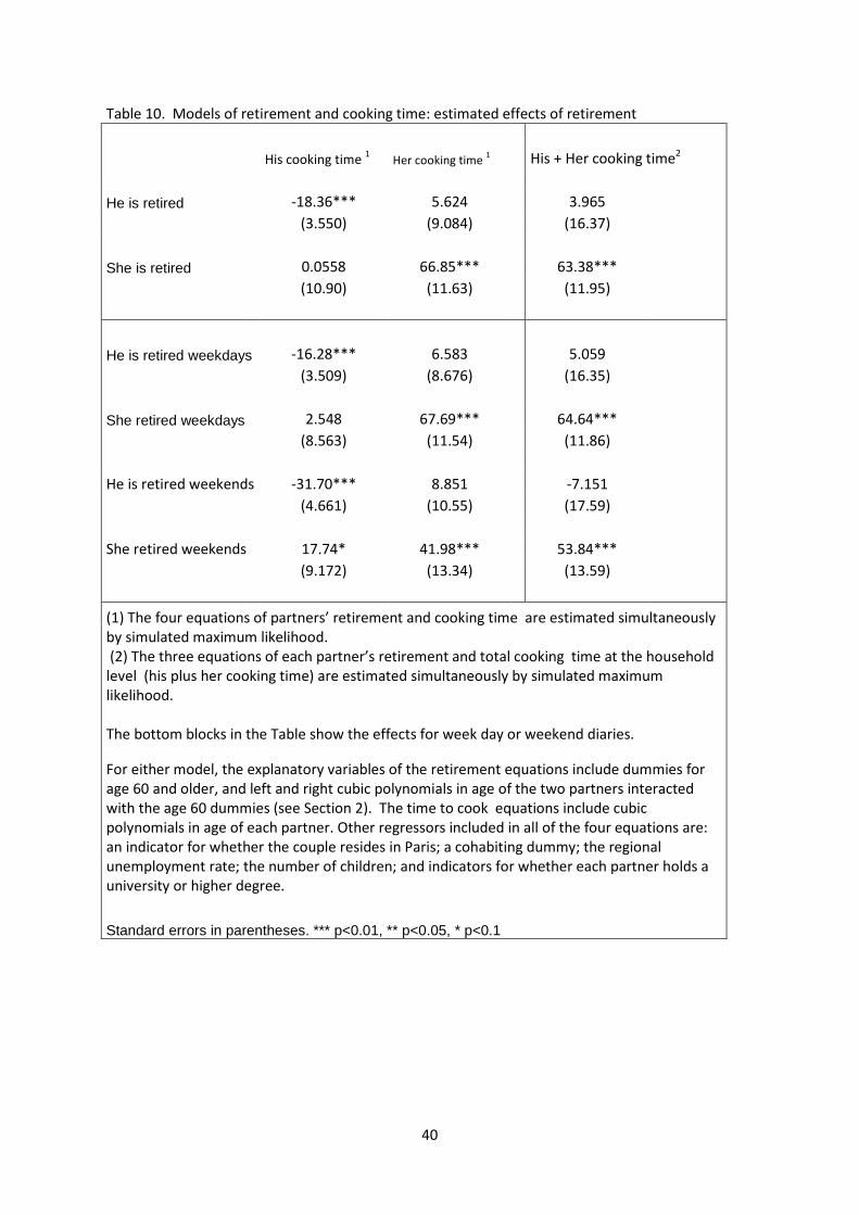
40

Table 10. Models of retirement and cooking time: estimated effects of retirement

His cooking time 1 Her cooking time

1

His + Her cooking time2

He is retired

-18.36*** 5.624 3.965

(3.550) (9.084) (16.37)

She is retired 0.0558 66.85*** 63.38***

(10.90) (11.63) (11.95)

He is retired weekdays -16.28*** 6.583 5.059

(3.509) (8.676) (16.35)

She retired weekdays 2.548 67.69*** 64.64***

(8.563) (11.54) (11.86)

He is retired weekends -31.70*** 8.851 -7.151

(4.661) (10.55) (17.59)

She retired weekends 17.74* 41.98*** 53.84***

(9.172) (13.34) (13.59)

(1) The four equations of partners’ retirement and cooking time are estimated simultaneously

by simulated maximum likelihood.

(2) The three equations of each partner’s retirement and total cooking time at the household

level (his plus her cooking time) are estimated simultaneously by simulated maximum

likelihood.




with the age 60 dummies (see Section 2). The time to cook equations include cubic






41

Table 11. Models of retirement and shopping time: estimated effects of retirement

His shopping time 1 Her shopping time

1

His + Her shopping time2

He is retired

-33.70*** -10.55 23.96

(8.866) (10.64) (30.04)

She is retired 27.07** 25.65 48.72**

(11.02) (17.02) (22.08)

He is retired weekdays -30.14*** -12.06 28.37

(8.223) (10.40) (32.02)

She retired weekdays 27.62** 29.62* 52.56**

(10.80) (17.24) (22.42)

He is retired weekends -58.45*** -13.98 1.145

(10.22) (12.20) (33.99)

She retired weekends 32.23*** 7.466 34.18

(12.09) (18.09) (24.26)

(1) The four equations of partners’ retirement and shopping time are estimated


(2) The three equations of each partner’s retirement and total shopping time at the

household level (his plus her cooking time) are estimated simultaneously by simulated

maximum likelihood.




with the age 60 dummies (see Section 2). The time to shop equations include cubic






42

Table12. Models of retirement and Care Time: estimated effects of retirement

His care time1 Her care time

1

His + Her Care time2

He is retired

34.30*** 13.97 51.20**

(11.47) (15.89) (20.04)

She is retired 13.63 30.49** 39.43*

(15.50) (12.60) (23.94)


(11.82) (16.26) (20.53)

She retired weekdays 13.08 31.75** 40.12*

(15.34) (12.92) (24.25)

He is retired weekends 18.22 9.986 30.64

(14.47) (18.56) (24.61)

She retired weekends 20.09 26.12* 41.44

(17.40) (15.32) (27.47)

(1) The four equations of partners’ retirement and care time are estimated simultaneously by


(2) The three equations of each partner’s retirement and total care time at the household

level (his plus her care time) are estimated simultaneously by simulated maximum likelihood.




with the age 60 dummies (see Section 2). The care equations include cubic polynomials in age

of each partner. Other regressors included in all of the four equations are: an indicator for

whether the couple resides in Paris; a cohabiting dummy; the regional unemployment rate;

the number of children; and indicators for whether each partner holds a university or higher

degree.

Care time includes child and adult care, to individuals from the same or from other households.


43

Table 13 Models of Paid Work and Home Production: estimated effects

His total

housework1

Her total

housework1

His + Her Total Housework2

His paid work time

-0.361** -0.150 -0.528**

(0.157) (0.141) (0.251)

Her paid work time 0.323 -0.295 0.0140

(0.238) (0.207) (0.377)

His paid work weekdays -0.437*** -0.0901 -0.529***

(0.1000) (0.0915) (0.158)

Her paid work weekdays 0.253 -0.313* -0.0589

(0.180) (0.163) (0.286)

His paid work weekends -0.319** 0.00258 -0.319

(0.129) (0.118) (0.203)

Her paid work weekends 0.463** -0.195 0.268

(0.199) (0.180) (0.314)

(1) The four equations of partners’ paid work and house work are estimated simultaneously by


(2) The three equations of each partner's paid work and total house work at the household level

(his plus her house work) are estimated simultaneously by simulated maximum likelihood.


For either model, the explanatory variables of the paid work equations include dummies for age 60

and older, and left and right cubic polynomials in age of the two partners interacted with the age 60

dummies a weekend day dummy also interacted with the age 60 dummies (see Section 2). The

house work equations include cubic polynomials in age of each partner. Other regressors included in

all of the four equations are: an indicator for whether the couple resides in Paris; a cohabiting

dummy; the regional unemployment rate; the number of children; and indicators for whether each

partner holds a university or higher degree.

House work includes semi-leisure chores, core chores, cooking and shopping.


44

Table 14. Models of Paid Work and ‘core’ chores : estimated effects

His core chores 1

Her core chores 1

His + Her core chores2

His paid work time

0.0444 -0.0517 0.0114

(0.0637) (0.103) (0.124)

Her paid work time 0.00338 0.0165 -0.00549

(0.0913) (0.160) (0.187)

His paid work weekdays

0.0104 -0.0549 -0.0350

(0.0418) (0.0654) (0.0790)

Her paid work weekdays -0.0234 -0.0311 -0.0746

(0.0735) (0.120) (0.143)

His paid work weekends

0.0127 0.0258 0.0471

(0.0550) (0.0826) (0.103)

Her paid work weekends

0.103 0.000222 0.0833

(0.0819) (0.130) (0.158)

(1) The four equations of partners’ paid work and core chores time are estimated simultaneously by


(2) The three equations of each partner's paid work and total core chores time at the household level

(his plus her core house work) are estimated simultaneously by simulated maximum likelihood.


For either model, the explanatory variables of the paid work equations include dummies for age 60 and

older, and left and right cubic polynomials in age of the two partners interacted with the age 60 dummies

and a weeken dummy interacted with age 60 of the two partners (see Section 2). The core house work

time equations include cubic polynomials in age of each partner. Other regressors included in all of the

four (three) equations are: an indicator for whether the couple resides in Paris; a cohabiting dummy; the

regional unemployment rate; the number of children; and indicators for whether each partner holds a


‘Core’ chores include cleaning, washing up dishes, doing the laundry and the ironing.


45

Table 15. Models of Paid Work and ‘semi-leisure’ house work: estimated effects

His semi-

leisure 1

Her semi-

leisure 1

His + Her semi-leisure

house work2

His paid work time

-0.265* -0.0985 -0.387**

(0.158) (0.0822) (0.180)

Her paid work time 0.392 -0.116 0.185

(0.254) (0.124) (0.261)


-0.346*** -0.0362 -0.375***

(0.0960) (0.0539) (0.118)

Her paid work weekdays 0.252 -0.0482 0.186

(0.176) (0.0960) (0.209)


-0.271** -0.0314 -0.296*

(0.121) (0.0709) (0.153)


0.370* -0.0153 0.337

(0.191) (0.107) (0.232)

(1) The four equations of partners’ paid work and ‘semi-leisure’ house work are estimated simultaneously

by simulated maximum likelihood.

(2) The three equations of each partner's paid work and total semi-leisure house work at the household

level (his plus her semi-leisure house work) are estimated simultaneously by simulated maximum

likelihood.



older, and left and right cubic polynomials in age of the two partners interacted with the age 60 dummies a

weekend day dummy also interacted with the age 60 dummies (see Section 2). The semi-leisure house

work equations include cubic polynomials in age of each partner. Other regressors included in all of the four

equations are: an indicator for whether the couple resides in Paris; a cohabiting dummy; the regional

unemployment rate; the number of children; and indicators for whether each partner holds a university or

higher degree.

‘Semi-leisure’ house work includes house repairs, gardening, knitting, sewing, making jams, care of pets.


46

Table 16. Models of Paid Work and cooking time: estimated effects

His cooking

time 1

Her cooking

time 1

His + Her cooking time2

His paid work time

-0.0406 -0.0109 -0.0516

(0.0267) (0.0504) (0.0565)

Her paid work time 0.0851** -0.0858 -0.0151

(0.0391) (0.0750) (0.0878)


-0.0390** 0.0206 -0.0147

(0.0174) (0.0348) (0.0382)

Her paid work weekdays 0.0793*** -0.147** -0.0776

(0.0308) (0.0635) (0.0726)


-0.0107 0.0243 0.0166

(0.0226) (0.0448) (0.0482)


0.0425 -0.131* -0.0990

(0.0341) (0.0702) (0.0792)

(1) The four equations of partners’ paid work and cooking time are estimated simultaneously by


(2) The three equations of each partner's paid work and total cooking time at the household level (his

plus her semi-leisure house work) are estimated simultaneously by simulated maximum likelihood.




(see Section 2). The time to cook equations include cubic polynomials in age of each partner. Other

regressors included in all of the four equations are: an indicator for whether the couple resides in Paris; a

cohabiting dummy; the regional unemployment rate; the number of children; and indicators for whether

each partner holds a university or higher degree.


47

Table17. Models of Paid Work and shopping time: estimated effects

His shopping

time 1

Her shopping

time 1

His + Her shopping time2

His paid work time

-0.0767 -0.00521 -0.0819

(0.0513) (0.0558) (0.0882)

Her paid work time -0.0527 -0.106 -0.164

(0.0729) (0.0821) (0.128)


-0.0716** -0.0217 -0.0911

(0.0333) (0.0364) (0.0567)

Her paid work weekdays -0.0331 -0.0813 -0.119

(0.0581) (0.0653) (0.100)


-0.0594 -0.0175 -0.0749

(0.0442) (0.0475) (0.0744)


-0.0299 -0.0443 -0.0790

(0.0654) (0.0727) (0.112)

(1) The four equations of partners’ paid work and shopping time are estimated simultaneously by


(2) The three equations of each partner's paid work and total shopping time at the household level (his

plus her semi-leisure house work) are estimated simultaneously by simulated maximum likelihood.




(see Section 2). The time to shop equations include cubic polynomials in age of each partner. Other

regressors included in all of the four (three) equations are: an indicator for whether the couple resides in

Paris; a cohabiting dummy; the regional unemployment rate; the number of children; and indicators for

whether each partner holds a university or higher degree.


48

Table 18 Models of Paid Work and Care Time: estimated effects

His care time1 Her care time

1

His + Her Total Care Time2

His paid work time

-0.264*** -0.134* -0.384***

(0.101) (0.0767) (0.141)

Her paid work time -0.114 -0.00809 -0.0318

(0.170) (0.109) (0.208)

His paid work weekdays -0.0920 -0.0857* -0.209**

(0.0583) (0.0499) (0.0852)

Her paid work weekdays -0.0740 0.0655 0.0796

(0.113) (0.0888) (0.158)

His paid work weekends -0.151** -0.152** -0.329***

(0.0713) (0.0641) (0.105)

Her paid work weekends -0.0694 0.137 0.155

(0.123) (0.0992) (0.172)

(1) The four equations of partners’ paid work and care time are estimated simultaneously by


(2) The three equations of each partner's paid work and total house work at the household level

(his plus her house work) are estimated simultaneously by simulated maximum likelihood.


For either model, the explanatory variables of the paid work equations include dummies for age 60

and older, and left and right cubic polynomials in age of the two partners interacted with the age 60

dummies a weekend day dummy also interacted with the age 60 dummies (see Section 2). The

house work equations include cubic polynomials in age of each partner. Other regressors included in

all of the four equations are: an indicator for whether the couple resides in Paris; a cohabiting

dummy; the regional unemployment rate; the number of children; and indicators for whether each

partner holds a university or higher degree.

House work includes ‘semi-leisure’ chores, ‘core’ chores, cooking and shopping.


Retirement and House Work: A Regression Discontinuity...

Documents

Transcript of Retirement and House Work: A Regression Discontinuity...